Global Description of Beta Decay with the Axially-Deformed Skyrme Finite Amplitude Method: Extension to Odd-Mass and Odd-Odd Nuclei

Abstract

We use the finite amplitude method (FAM), an efficient implementation of the quasiparticle random phase approximation, to compute beta-decay rates with Skyrme energy-density functionals for 3983 nuclei, essentially all the medium-mass and heavy isotopes on the neutron rich side of stability. We employ an extension of the FAM that treats odd-mass and odd-odd nuclear ground states in the equal filling approximation. Our rates are in reasonable agreement both with experimental data where available and with rates from other global calculations.

I Introduction

The origin of elements heavier than iron still remains an open question. Early work has shown that neutron capture in astrophysical processes is responsible for synthesizing those elements Burbidge et al. (1957); Meyer (1994). Rapid neutron capture, through the “$r$-process,” is particularly interesting because its astrophysical site is still uncertain. The multi-messenger neutron star merger GW170817 LIGO Scientific Collaboration and Virgo Collaboration (2017) recently provided evidence that such events are the dominant source of $r$-process elements, but quantitative conclusions require more data. We need more reliable astrophysical simulations to connect future multi-messenger events with details of the underlying nucleosynthesis.

Abundances of $r$-process elements depend on a variety of nuclear properties, including masses, neutron-capture cross sections, photo-disintegration cross sections, fission yields, and beta-decay half-lives Horowitz et al. (2019). Although some of these properties have been measured and tabulated Evaluated Nuclear Structure Data File (2019) (ENSDF), the majority of nuclei relevant for the $r$-process are too unstable to be produced in the lab. Reliable $r$-process simulations thus require calculations in neutron-rich nuclei. Beta-decay half-lives are particularly important because they determine the overall timescale for neutron capture in the $r$-process Möller et al. (1997); Engel et al. (1999) and affect the shape of the final abundance pattern Mumpower et al. (2014); Shafer et al. (2016).

A variety of global beta-decay calculations exist, in the semi-gross theory Nakata et al. (1997), in a quasiparticle random-phase approximation (QRPA) plus macroscopic finite-range droplet model (FRDM) approach Möller et al. (1997, 2003), in covariant density functional theory (DFT) Marketin et al. (2016), etc. DFT, covariant or not, is particularly attractive because it offers a self-consistent, microscopic framework for computing properties across the nuclear chart Ring and Schuck (2004); Schunck (2019). For the calculation of beta decay in deformed superfluid nuclei, DFT amounts to the QRPA, built on a ground state produced by the Hartree-Fock-Bogoliubov (HFB) method, which incorporates pairing correlations into mean fields, all with density-dependent interactions.

In odd-mass and odd-odd nuclei (hereafter “odd” nuclei) pairing is “blocked” and the HFB ground-state contains a quasiparticle excitation Ring and Schuck (2004). This complicates calculations because the ground-state is no longer invariant under time reversal Bertsch et al. (2009a); Schunck et al. (2010). As a result additional approximations are often made in beta-decay calculations. Reference Homma et al. (1996), for example, treats one-quasiparticle states perturbatively, while Ref. Marketin et al. (2016) treats them as if they were zero-quasiparticle states. A more consistent way to approximate HFB blocked states while preserving time-reversal symmetry is through the equal filling approximation (EFA) Perez-Martin and Robledo (2008). Numerous studies showed that the EFA is an excellent approximation to exact blocking Duguet et al. (2001); Bertsch et al. (2009b); Schunck et al. (2010). Reference Shafer et al. (2016) recently developed a method to extend the EFA to the QRPA.

In this work we use the extension to carry out a global calculation of allowed and first-forbidden contributions to beta-minus decay in odd nuclei from near the valley of stability out to the neutron drip line. We use a global Skyrme density functional determined in Ref. Mustonen and Engel (2016), thus extending that work, which was restricted to even-even nuclei, to all isotopes that play a role in the $r$-process.

This rest of this paper is as follows: Sec. II presents background for the finite amplitude method (FAM), which we use to compute QRPA strength functions, and its extension to the EFA. Section III outlines some improvements to our implementation of the FAM since the work of Ref. Mustonen and Engel (2016). Section IV presents our results, compares them to those of other papers and to experiment, and addresses subtleties of the EFA-FAM. Section V contains concluding remarks.

II The proton-neutron finite amplitude method (pnFAM)

II.1 The pnFAM for pure states

The QRPA linear-response function is the same as that from time-dependent HFB theory Ring and Schuck (2004). One way of computing it is to diagonalize a set of matrices with dimension equal to that of the two-quasiparticle space. The construction of these matrices, which require two-body matrix elements of the potential, is time consuming in deformed nuclei. The FAM sidesteps the matrices, significantly speeding up the computation of linear response produced by energy-density functionals. Reference Nakatsukasa et al. (2007) first presented the FAM for the ordinary RPA, and Ref. Avogadro and Nakatsukasa (2011) did the same for the QRPA. Since then, the method has been used with covariant density functionals Nikšić et al. (2013); Liang et al. (2013, 2014) and employed to compute transition strength in several contexts Inakura et al. (2009a, b, 2010); Stoitsov et al. (2011); Oishi et al. (2016).

Here we build on the work of Refs. Mustonen et al. (2014); Mustonen and Engel (2016); Shafer et al. (2016), which used a charge-changing version of the FAM called the pnFAM together with the contour-integral method of Refs. Nakatsukasa (2014); Hinohara (2015); Hinohara et al. (2013, 2015) to compute beta-decay rates. A detailed account of the pnFAM and its application to beta decay appears in Ref. Mustonen et al. (2014). Reference Shafer et al. (2016) used the EFA to extend the pnFAM to odd nuclei and compute beta-decay rates in the rare-earth nuclei that are important for $r$-process simulations. In order to highlight a few subtleties of the EFA-pnFAM, we recapitulate the main points of the theory here.

We begin with the time-dependent HFB equations

$$i\dot{\mathbb{R}}(t)=\big{[}\mathbb{H}[\mathbb{R}(t)]+\mathbb{F}(t),\ \mathbb{R}(t)\big{]}\,.$$ (1)

Here, $\mathbb{R}$ is the generalized HFB density matrix, $\mathbb{H}$ is the HFB Hamiltonian matrix, and $\mathbb{F}$ is a matrix that represents a one-body time-dependent perturbation. The blackboard-bold letters indicate that these matrices are in the HFB quasiparticle basis, defined by the Bogoliubov transformation $\mathbb{W}$:

$$\mathbb{W}=\begin{pmatrix}U&V^{*}\\ V&U^{*}\end{pmatrix}\,,$$ (2)

where $U$ and $V$ are themselves matrices. In this basis the static ground-state Hamiltonian and the associated generalized density are diagonal:

$$\mathbb{H}_{0}=\begin{pmatrix}E&0\\ 0&-E\end{pmatrix}\,,\quad\mathbb{R}_{0}=\begin{pmatrix}0&0\\ 0&1\end{pmatrix}\,.$$ (3)

To first order in the perturbation $\mathbb{F}$, Eq. (1) is

$$i\dot{\delta\mathbb{R}}(t)=\big{[}\mathbb{H}_{0},\delta\mathbb{R}(t)\big{]}+\big{[}\delta\mathbb{H}(t)+\mathbb{F}(t),\mathbb{R}_{0}\big{]}\,,$$ (4)

with $\delta\mathbb{R}(t)=\mathbb{R}(t)-\mathbb{R}_{0}$. If the perturbation is harmonic, the time-dependent quantities $\mathbb{F}(t)$, $\delta\mathbb{H}(t)$, and $\delta\mathbb{R}(t)$ all take the form (e.g. for $\mathbb{F}$)

$$\mathbb{F}(t) =\mathbb{F}(\omega)e^{-i\omega t}+\mathbb{F}^{\dagger}(\omega)e^{i\omega t}$$ (5)

$$\mathbb{F}(\omega) =\begin{pmatrix}{F}^{11}(\omega)&{F}^{02}(\omega)\\ -{F}^{20}(\omega)&-{F}^{\overline{11}}(\omega)\end{pmatrix}\,.$$

We denote the perturbed density more specifically by

$$\delta\mathbb{R}(\omega)=\begin{pmatrix}P(\omega)&X(\omega)\\ -Y(\omega)&-Q(\omega)\end{pmatrix}\,.$$ (6)

When one substitutes Eqs. (5) and (6) into Eq. (4), the diagonal blocks $P$ and $Q$ vanish, and for a charge-changing external field only the proton-neutron matrix elements of the response are nonzero. These conditions lead to the pnFAM equations

$$\big{(}E_{\pi}+E_{\nu}-\omega\big{)}X_{\pi\nu}(\omega)=-\big{(}\delta{H}^{20}_{\pi\nu}(\omega)+{F}^{20}_{\pi\nu}(\omega)\big{)}$$ (7)

$$\big{(}E_{\pi}+E_{\nu}+\omega\big{)}\ Y_{\pi\nu}(\omega)=-\big{(}\delta{H}^{02}_{\pi\nu}(\omega)+{F}^{02}_{\pi\nu}(\omega)\big{)}\,,$$

where the label $\pi$ denotes protons and the label $\nu$ denotes neutrons. The use of a finite-difference method to compute $\delta{H}$ is the source of the FAM’s speed. Because we do not consider mixing of protons and neutrons in the underlying HFB ground state, and because Skyrme functionals in use depend at most quadratically on charge-changing densities, the finite difference in the pnFAM reduces exactly to the evaluation of the Hamiltonian with the perturbed densities:

$$\delta\mathbb{H}^{(pn)} =\lim_{\eta\to 0}\frac{1}{\eta}\bigg{(}\mathbb{H}\Big{[}\mathbb{R}_{0}^{(pp,nn)}+\eta\delta\mathbb{R}^{(pn)}\Big{]}-\mathbb{H}\Big{[}\mathbb{R}_{0}^{(pp,nn)}\Big{]}\bigg{)}$$ (8)

$$=\mathbb{H}\Big{[}\delta\mathbb{R}^{(pn)}\Big{]}\,.$$

Once the FAM amplitudes $X$ and $Y$ are known, one can compute the strength function:

$$\frac{dB(F,\omega)}{d\omega}=-\frac{1}{\pi}\imaginary S(F,\omega)\,,$$ (9)

where

$$S(F,\omega) =\sum\limits_{\pi\nu}\big{[}{F}^{20^{*}}_{\pi\nu}X_{\pi\nu}(\omega)+{F}^{02^{*}}_{\pi\nu}Y_{\pi\nu}(\omega)\big{]}$$ (10)

$$=-\sum\limits_{n}\bigg{(}\frac{\lvert\bra{n}\hat{F}\ket{0}\rvert^{2}}{\Omega_{n}-\omega}+\frac{\lvert\bra{n}\hat{F}^{\dagger}\ket{0}\rvert^{2}}{\Omega_{n}+\omega}\bigg{)}\,.$$

The FAM strength function has poles at QRPA excitation energies $\Omega_{n}$ with residues equal to the transition probabilities $\lvert\bra{n}\hat{F}\ket{0}\rvert^{2}$. It also contains poles at $-\Omega_{n}$, with residues equal to the negative of transition probabilities for the conjugate operator $\lvert\bra{n}\hat{F}^{\dagger}\ket{0}\rvert^{2}$. In beta-minus-decay calculations $\hat{F}$ contains the isospin lowering operator and $\hat{F}^{\dagger}$ contains the isospin raising operator; cf. Ref. Mustonen et al. (2014) for a list of the six allowed and first-forbidden operators. Thus, the poles with positive and negative residues correspond to beta-minus and beta-plus transitions, respectively. This point will become important in the EFA-pnFAM.

In practice we construct the strength function by solving the pnFAM equations separately for each of a large set of complex frequencies $\omega$. From Eqs. (9) and (10), it is straightforward to show that each pole of $S(F,\omega)$ on the real axis contributes a Lorentzian of half-width $\gamma=\imaginary[\omega]$ to the strength function in the complex plane. The strength may be be calculated for a set of frequencies close to the real axis with a fixed half-width to mimic experimental strength measurements, or along a closed contour in the complex plane to calculate cumulative strength or decay rates.

II.2 The pnFAM for statistical ensembles

Many HFB codes use the EFA to avoid the difficulties associated with the breaking of time-reversal symmetry Ring and Schuck (2004); Bertsch et al. (2009a) in odd nuclei. The originally ad hoc EFA can be understood as a special case of statistical HFB theory for an ensemble that is symmetric under time reversal Perez-Martin and Robledo (2008); Schunck et al. (2010). In systems with time-reversal symmetry, a state $\ket{\lambda}$ and its time-reversed partner $\ket{\overline{\lambda}}$ are degenerate, and the equal filling quasiparticle occupation probabilities, for axial but not spherical symmetry, are

$$f_{\mu\nu}=\frac{1}{2}(\delta_{\nu\lambda}+\delta_{\nu\overline{\lambda}})\delta_{\mu\nu}\,.$$ (11)

In odd-odd nuclei, both the odd-proton and odd-neutron quasiparticles have non-zero occupation probabilities. Note that in this work, we do not consider neutron-proton pairing at the HFB level.

The statistical extension of the QRPA Sommermann (1983) lets us use the FAM to treat excitations of HFB ensembles, taking into account at least partially the polarization of the even-even “core” by the odd nucleon. The EFA-FAM can be derived in the same way as the ordinary FAM, by promoting the ground-state generalized density matrix to a statistical density operator. Expectation values that, for example, define the particle densities, then become ensemble averages. The generalized HFB density matrix is no longer a projector and takes the more general form

$$\widetilde{\mathbb{R}}_{0}=\begin{pmatrix}f&0\\ 0&1-f\end{pmatrix}\,.$$ (12)

In the usual finite-temperature theory, based on the grand canonical ensemble, the occupation probabilities are given by $f_{\mu\nu}={(1+\exp(\beta E_{\mu}))^{-1}}\delta_{\mu\nu}$ Goodman (1981). In the EFA we impose the occupation probabilities of Eq. (11).

To obtain the statistical pnFAM equations we simply replace the ground-state generalized density of Sec. II.1 with that of Eq. (12). The diagonal elements of the density response no longer vanish, and new statistical factors appear. Once again, for a charge-changing perturbation we need only the proton-neutron matrix elements, and so the statistical pnFAM equations are

$$\big{(}E_{\pi}-E_{\nu}-\omega\big{)}P_{\pi\nu}(\omega)=-(f_{\nu}-f_{\pi})\big{(}\delta{H}+{F}\big{)}^{11}_{\pi\nu}(\omega)$$ (13)

$$\big{(}E_{\pi}+E_{\nu}-\omega\big{)}X_{\pi\nu}(\omega)=-(1-f_{\pi}-f_{\nu})\big{(}\delta{H}+{F}\big{)}^{20}_{\pi\nu}(\omega)$$

$$\big{(}E_{\pi}+E_{\nu}+\omega\big{)}Y_{\pi\nu}(\omega)=-(1-f_{\pi}-f_{\nu})\big{(}\delta{H}+{F}\big{)}^{02}_{\pi\nu}(\omega)$$

$$\big{(}E_{\pi}-E_{\nu}+\omega\big{)}Q_{\pi\nu}(\omega)=-(f_{\nu}-f_{\pi})\big{(}\delta{H}+{F}\big{)}^{\overline{11}}_{\pi\nu}(\omega)\,.$$

The additional $P$ and $Q$ amplitudes arise because the non-zero occupation probabilities allow quasiparticles to be destroyed as well as created. The new transitions introduce an additional set of QRPA eigenvalues that contain quasiparticle-energy differences rather than sums Sommermann (1983). It is possible for these energy differences to be negative, indicating a transition to a state of lower energy. This does not mean, however, that the QRPA fails, as it does when the eigenvalues are imaginary. The statistical FAM strength has the same form as the usual strength in Eq. (10), but the residues become ensemble-averaged transition strengths, and $n$ runs over the expanded set of QRPA modes. More details on the EFA-FAM and a demonstration that it includes all necessary transitions for odd states, in the context of the particle-rotor model Bohr and Mottelson (1998), appear in Ref. Shafer et al. (2016).

III Computational method

III.1 HFB ground states and functional

In obtaining our global set of half-lives, we introduce a number of small improvements to the procedure of Ref. Mustonen and Engel (2016), in addition to the changes required to compute half-lives of odd nuclei. The first is in the determination of the HFB ground state/ensemble. To make sure that we identify the correct ground state, we perform three different calculations for each even-even nucleus by constraining the first ten iterations of the HFB solver to an oblate, spherical and prolate quadrupole shape before releasing the constraint. In contrast to Ref. Mustonen and Engel (2016), which used a set of three fixed quadrupole constraints for all nuclei, we use the first-order mass-dependent relation Ring and Schuck (2004)

$$Q_{2}=\frac{5}{100\pi}\beta_{2}A^{5/3}\,,$$ (14)

with values $\beta_{2}=-0.2,0.0,+0.2$. This procedure gives one, two or three different deformed minima, depending on the even-even nucleus. We then identify a number of candidate quasiparticle states within 1 MeV of the Fermi surface to block in the EFA. For odd-odd nuclei we consider all possible combinations of proton and neutron candidates. For every candidate (or candidate pair), we carry out the EFA on top of each available deformed even-even core, without constraints, and select the solution with the lowest energy. On occasion these are meta-stable super-deformed states, which we discard.

We use the Skyrme functional SKO^′ Reinhard et al. (1999), which was found in Ref Mustonen and Engel (2016) to give accurate $Q$-values across the nuclear chart. We fit the like-particle pairing strengths to the experimental pairing gaps of ten isotopes picked in a wide mass range $50\leq A\leq 230$, and apply an ulta-violet cutoff of 60 MeV to the single particle space. For the pnFAM portion of the calculation we set the time-odd parameters and isoscalar pairing strength to the values determined in the fit “1A” of that reference. We therefore also use the same 16-shell deformed harmonic-oscillator basis that was used in the original fit. All HFB calculations are performed with the latest version of the hfbtho code Perez et al. (2017).

III.2 Beta-decay half-lives

The next set of changes concerns the computation of the beta-decay half-lives, which is discussed in detail in Ref. Mustonen et al. (2014). The procedure therein allows us to sum the phase-space-weighted strengths to all energetically allowed daughter states. For allowed transitions, we obtain the rate and half-life via

$$\lambda=\frac{\ln 2}{\kappa}\sum\limits_{n}f(W_{n})\lvert\bra{n}F\ket{0}\rvert^{2},\quad t_{1/2}=\frac{\ln 2}{\lambda}\,,$$ (15)

where $\ket{n}$ is the $n^{\text{th}}$ state in the daughter nucleus, ${W_{n}=E_{n}/m_{e}c^{2}}$ is the energy, in units of electron mass, of the electron emitted during a transition to that state, and $\kappa=6147.0\pm 2.4s$. To include first-forbidden transitions, we must consider a more complicated phase-space-weighted “shape factor” Mustonen et al. (2014). We evaluate the right side of the first relation in Eq. (15) by integrating the phase-space-weighted strength (Eq. (10)) along a circular complex energy contour Mustonen et al. (2014) that encloses all the poles below the decay $Q$-value. Because the phase-space integral $f(W_{n})$ is not analytic, the authors of Ref. Mustonen et al. (2014) fit a polynomial to the integrals on the real axis, and analytically continued the polynomial. High-degree polynomials on evenly spaced grids, however, exhibit the Runge-phenomenon Runge (1901), and can oscillate rapidly in the complex plane. We therefore elect here to use a rational function to interpolate the phase-space integrals on a 20-point Chebychev grid. Because the contour integrand is quite smooth, we use Gauss-Legendre quadrature to perform the contour integration.

The maximum QRPA energy relevant for beta decay defines the right bound of the circular energy contour. With the treatment of $Q$-values in Refs. Engel et al. (1999); Mustonen et al. (2014); Shafer et al. (2016), the energy released in the transition to the $n^{th}$ excited state in the daughter nucleus is

$$Q_{\beta}^{(n)}=\Delta M_{n-H}+\lambda_{n}-\lambda_{p}-\Omega_{n}\,,$$ (16)

where $\Delta M_{n-H}$ is the neutron-hydrogen mass difference, $\lambda_{p}$ and $\lambda_{n}$ are the proton and neutron HFB Fermi energies, and $\Omega_{n}$ ($n\geq 1$) is the excitation energy of the $n^{\rm th}$ QRPA mode above the initial-nucleus ground state, after adjustment by the Fermi energies for the change in particle number. (Note that $\Omega_{1}$ is the “excitation energy” of the ground state of the daughter nucleus.) The maximum QRPA energy, which corresponds to an energy release of zero is then the excitation energy of, e.g., the daughter ground state plus the energy released in the transition to that state,

$$E_{\rm max}^{\rm QRPA}=Q_{\beta}^{(1)}+\Omega_{1}=\Delta M_{n-H}+\lambda_{n}-\lambda_{p}\,.$$ (17)

and can be evaluated without knowing the daughter ground-state energy itself.

The left bound of the circular energy contour must still be chosen. It must be less than $\Omega_{1}$, which we do not know exactly, to include all relevant poles in the response. For even-even parent nuclei we can always choose it to be zero because pairing correlations always make $\Omega_{1}$ positive. For odd parent nuclei, however, $\Omega_{1}$ can be negative. If we neglect the effects of the QRPA residual interaction, we find explicitly that

$$\Omega_{1}^{\text{even}} \approx E_{\pi}^{\text{smallest}}+E_{\nu}^{\text{smallest}}$$ (18)

$$\Omega_{1}^{\text{n-odd}} \approx E_{\pi}^{\text{smallest}}-E_{\nu}^{\text{blocked}}$$

$$\Omega_{1}^{\text{p-odd}} \approx E_{\nu}^{\text{smallest}}-E_{\pi}^{\text{blocked}}$$

$$\Omega_{1}^{\text{odd-odd}} \approx\text{min}\big{[}\Omega_{1}^{\text{p-odd}},\ \Omega_{1}^{\text{n-odd}}\big{]}\,.$$

The fact that $\Omega_{1}$ can be negative makes it difficult to choose the left bound. If we expand the contour arbitrarily, we risk including beta-plus poles with non-negligible negative strength, but if we do not expand it enough, the QRPA residual interaction places $\Omega_{1}$ outside the contour. Because the pnFAM produces the strength function in Eq. (9) directly, we do not have access to the underlying QRPA eigenvectors and therefore cannot separate beta-minus poles from beta-plus poles. Both the inclusion of beta-plus poles or the accidental exclusion of beta-minus poles at negative energies can cause the contour integration to artificially reduce the integrated (and phase-space-weighted) beta-minus strength, and therefore artificially increase the half-lives. For lack of a better prescription, we initially choose the left bound of the contour to be

$$E^{\text{QRPA}}_{\text{min}}=\text{min}\big{[}0,\Omega_{1}]\,,$$ (19)

with $\Omega_{1}$ given by the approximations in Eq. (18), but correct the rates as described below when the contour integration appears to lead to errors.

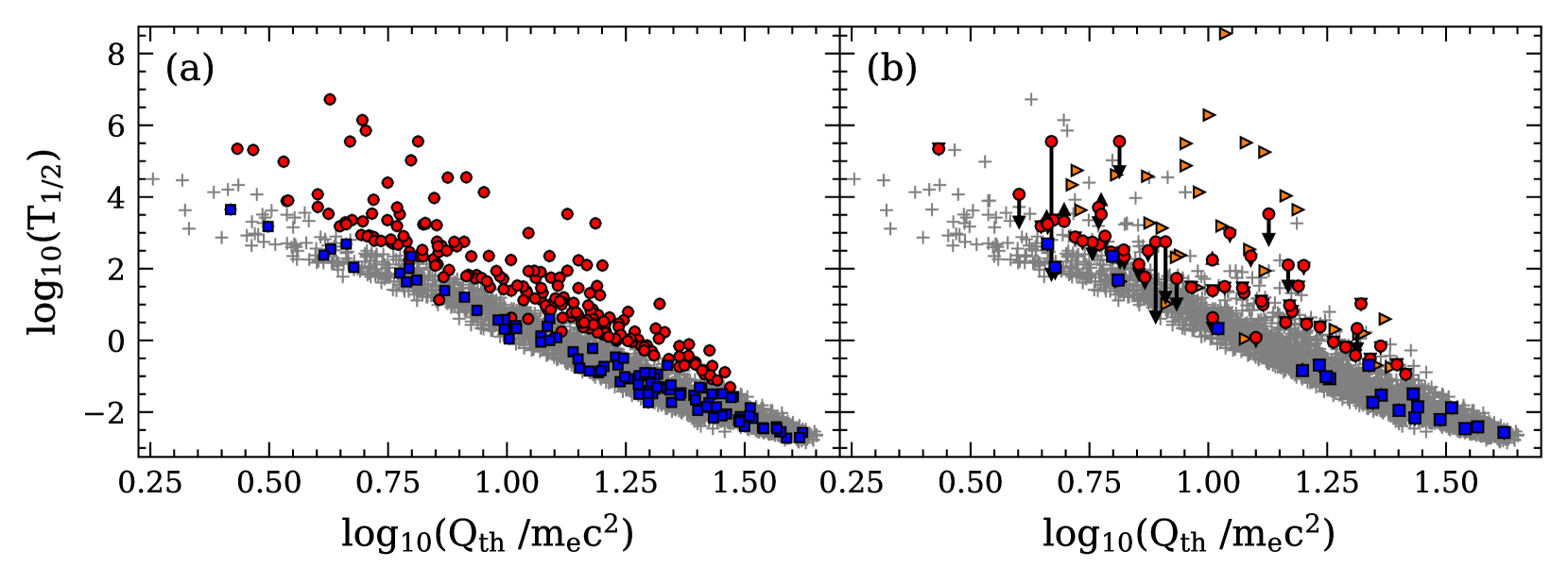
Figure 1: Corrections of half-lives in odd nuclei. Half-lives for which we calculate strength functions are in panel a). Red circles are for the 224 suspicious nuclei and blue squares for the 100 nuclei from the random sample. Panel b) shows half-lives that are corrected as described in the main text, with corrected values indicated by black arrowheads. Orange triangles are corrected versions of originally negative half-lives.

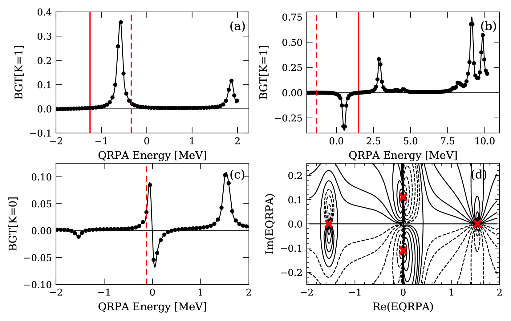
Figure 2: Examples in which contour integration fails. The dashed vertical line indicates the left bound of the contour from Eq. (18), while the solid line indicates the adjusted bound required to correct the rate. Panels a) and b) show the Gamow-Teller (K=1) strength function for ⁶³Co and ⁵³Sc, respectively. Panel c) illustrates an imaginary pole in the response function of ¹⁷³Er, and d) shows the response in the full complex plane, indicating poles near $\omega=\pm 0.1i$.

IV Results

IV.1 Half-lives and odd-nucleus subtleties

To carry out our calculations we bundle the HFB code hfbtho and the charge-changing FAM code pnfam together with a controlling python code called p${}_{\textsc{Y}}$nfam. We calculate the beta-minus decay half-lives of nuclei on the neutron rich side of stability, from $Z=20$ to $Z=110$, out to the one-neutron drip line. The lightest nuclei in each isotopic chain are near $A=50$, and coincide with those used in the global even-even calculation of Ref. Mustonen and Engel (2016). We obtain 3983 ground states, 2998 of which are odd isotopes. Reference Mustonen and Engel (2016), which included results to the two-neutron drip line, obtained 1387 even-even ground states with the same functional, versus our 985. Our computation consumed roughly 270,000 Xeon core hours.

Our results in even-even nuclei agree very closely with those of Ref. Mustonen and Engel (2016), with a few improvements that can be attributed to our updated procedures. As mentioned in Sec. III.2, however, our contour-integration result may be inaccurate in odd nuclei if $\Omega_{1}$ is less than zero. To assess the validity of the contour integration, we calculate strength functions near the real axis. Though this is a more time-consuming calculation, it allows us to locate beta-minus and beta-plus poles, determine if there are errors in the contour integration, and decide how to correct incorrect half-lives.

We identify two subsets of nuclei, shown in Fig. 1 panel a), for which we perform this additional calculation. The first, indicated by red circles, is a set of 224 odd nuclei that have decay rates significantly below the average for a given $Q$-value or that contain significant negative contributions. We refer to this set as “suspicious.” The second, shown with blue squares, is a random sample of 100 odd nuclei from the remaining population. Assuming that the probability of a half-life requiring correction is uniformly distributed, this sample size allows us to estimate the proportion of half-lives that require correction with a 10% margin of error at a 95% confidence level. We find that more than half of the examined lifetimes turn out to be correct, and those that are not contain errors of two types.

The first type, illustrated by the top panels of Fig. 2, can be corrected by simply shifting the left bound of the contour. In the figure, the original left bound (Eq. (19)) is the dashed vertical line, while the corrected left bound is the solid vertical line. There are two situations which cause this type of error. The first, similar to that shown in Fig. 2 panel b), occurs when the HFB estimate $\Omega_{1}$ is negative but the residual interaction moves it to a positive number $E<\lvert\Omega_{1}\rvert$. This is corrected by placing the left bound at zero. The second, illustrated in panels a) and b) of Fig. 2, occurs when there exists a beta-minus (beta-plus) transition at negative (positive) energy, but either the corresponding beta-minus or beta-plus strength itself is negligible. This behavior occurs almost exclusively in odd nuclei adjacent to closed shells, where pairing vanishes and the transition that takes the parent farther from the closed shell is suppressed. These cases are corrected by shifting the contour to exclude (include) beta-minus (beta-plus) poles with negligible strength.

The second type of error, exemplified by panel c) of Fig. 2, is more difficult to correct. Two situations can give rise to this shape in the strength distribution: the existence of a non-negligible beta-minus pole at negative energy and an associated non-negligible beta-plus pole at positive energy, or, as in panels c) and d), the existence of poles at imaginary energies. To determine if any corrections are warranted, we pinpoint the location of the poles by calculating the strength parallel to the imaginary axis out to 1 MeV. We examine the strength in each multipole, and if the original contour integration contains any errors, we integrate along a contour that surrounds only the problematic poles (and only them) to determine the correction.

We identify 60 nuclei — 54 in the suspicious set and 6 in the random sample — that require only a simple adjustment of the contour, and 41 nuclei — 26 in the suspicious set and 15 in the random sample — that require more careful corrections (33 of which have an imaginary pole in at least one multipole). The results of correcting the half-lives appear in panel b) of Fig. 1. The amount of change is indicated by the black arrowheads. Most of the arrowheads lie hidden beneath the circles or squares, usually because the problems are in forbidden multipoles that contribute only a small amount to the rate. Only a few half-lives shrink by more than an order of magnitude, when a low-lying beta-minus transition is missing from the original contour. Some half-lives increase slightly after we remove positive contributions from imaginary poles. Orange triangles in panel b) correspond to nuclei with negative total decay rates that became positive after correction.

Our random sample suggests that about 6% of our unexamined results should be corrected simply, by shifting the left bound of the contour, and about 15% may require more intricate corrections. Only a single half-life in the random sample changes by more than 5%, however (it changes by 30%). Thus, the corrections to unverified half-lives are very likely small compared to the average error in our rates (see Fig. 5). Nuclei with half-lives that require significant correction very probably belong to the suspicious set that we have just analyzed.

Finally, we should mention that numerical error is an additional source of small negative contributions to rates. Both the HFB and FAM solutions contain numerical error from several sources, e.g., incomplete convergence, truncation, etc. These errors are compounded in the final strength function and amplified by the phase space. If a rate is very small, the contour integral that generates it can suffer from incomplete cancellation of large oscillations. In compiling our final table of half-lives, presented here as supplemental material sup , we break each rate into contributions from each multipole, set any negative contributions to zero, and re-sum. This procedure usually changes rates by less than $5\%$.

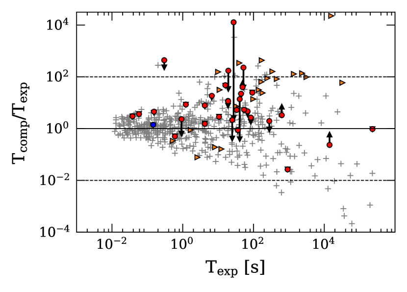
Figure 3: Same as panel b) of Fig. 1 but compared with 2019 ENSDF data. Only odd nuclei are shown.

In Fig. 3 we compare our final results with 2019 ENSDF experimental data Evaluated Nuclear Structure Data File (2019) (ENSDF) for nuclei with experimental half-lives less than $10^{6}$ s. We highlight half-lives that are corrected, as in Fig. 1 panel b), and find that corrections almost always improve the agreement with experiment. The majority of our data fall within one or two orders of magnitude of experiment for half-lives less than 1000 s. In the next section, we will quantify more rigorously the theoretical uncertainties associated with such calculations.

Figure 4 displays the contributions to decay rates of first-forbidden operators. We find, as do other groups, that first-forbidden contributions are important in many nuclei and observe competing effects: forbidden contributions scale with the nuclear radius and $Q$-value, becoming important in heavier nuclei far from stability, but they also become important near stability and closed shells where the allowed rate is very small and allowed contributions are suppressed.

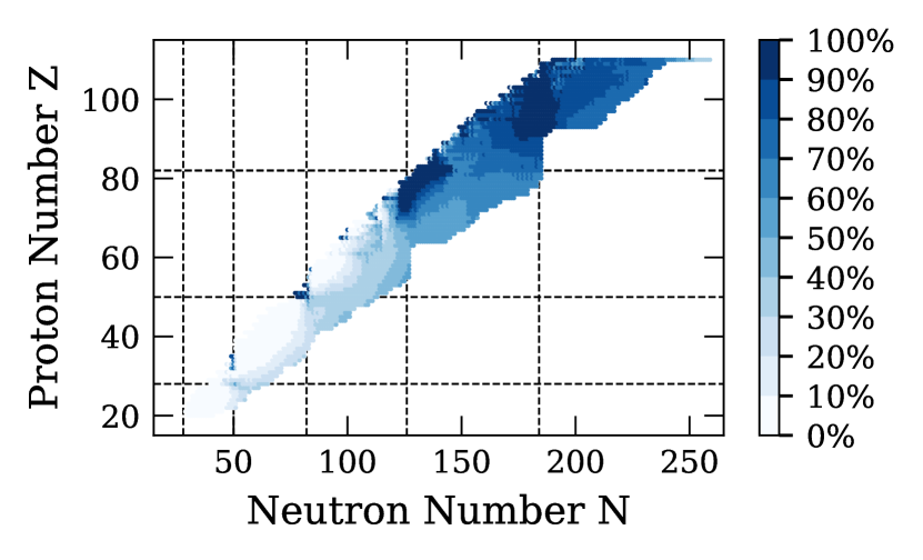
Figure 4: First-forbidden contribution to the rates.

IV.2 Error analysis

One major challenge facing large scale calculations is the quantification of uncertainty. Most of the nuclei considered here are not experimentally accessible, and so we lack an experimental benchmark with which to evaluate our calculations. A simple way to deal with this challenge is to develop a model for the error. The model can be fit to data where available, and then extrapolated or interpolated to estimate errors for the remaining data. We use the simple model developed in Ref. Mustonen and Engel (2016), which we summarize here. The error parameter of interest is, for the $i^{th}$ nucleus Möller et al. (2003),

$$r_{i}=\log_{10}\bigg{(}\frac{t_{\text{th}}}{t_{\text{exp}}}\bigg{)}\,.$$ (20)

To motivate a regression model for this parameter, we assume that there is a single dominant transition to a state near the daughter ground state, and that the forbidden shape factors depend much less on the $Q$-value than does the allowed phase space. These assumptions allow us to assign a single effective $Q$-value and shape factor $C_{\rm eff}$ to the decay; cf. Mustonen et al. (2014) for the definition of the shape factor $C$. Using $q_{\rm eff}$ to denote the effective $Q$-value in units of electron mass ($q_{\rm eff}=Q_{\rm eff}/m_{e}c^{2}$), we model the error $r_{i}$ on the rate, as a function of the theoretical $Q$-value and charge of the daughter nucleus, as,

$$r_{i}(q_{\text{g.s.}}^{\text{th}},Z_{f})\approx c_{r_{i}}+f_{r}(q_{\text{g.s.}}^{\text{th}}+1,Z_{f})q_{r_{i}}\,,$$ (21)

where the errors in the effective shape factor, $c_{r}$, and the effective $Q$-value, $q_{r}$, are defined by

$$c_{r}\equiv\log_{10}\frac{C^{\text{exp}}_{\text{eff}}}{C^{\text{th}}_{\text{eff}}},\quad q_{r}\equiv\frac{q_{{\text{eff}}}^{{\text{exp}}}-q_{\text{eff}}^{\text{th}}}{\ln 10}\,,$$ (22)

and the $Q$-value dependence is carried by the phase space factor,

$$f_{r}(q+1,Z_{f})\equiv\frac{1}{f(q+1,Z_{f})}\frac{df(q+1,Z_{f})}{dq}\,.$$ (23)

Next, we assume that the $c_{r_{i}}$ and $q_{r_{i}}$, which depend on the nucleus $i$, are each normally distributed random variables with widths that are independent of the $Q$-value, and that the distributions for $c_{r_{i}}$ and $q_{r_{i}}$ contain a systematic bias that is independent of the nucleus and the $Q$-value. These assumptions allow us to write the error parameters for nucleus $i$ in the form

$$c_{r_{i}} =b_{c}+\epsilon_{c},\quad\epsilon_{c}\sim\mathcal{N}(0,\sigma_{c})\,,$$ (24)

$$q_{r_{i}} =b_{q}+\epsilon_{q},\quad\epsilon_{c}\sim\mathcal{N}(0,\sigma_{q})\,,$$

where $b_{c},b_{q},\sigma_{c},\sigma_{q}$ are still undetermined parameters. Finally, since the assumptions of the model are best for large $Q$-values, we can make use of the Primakoff-Rosen approximation to the allowed phase space Suhonen (2007), which lets us express $f_{r}(q+1,Z_{f})$ as a simple rational function with no explicit dependence on the charge $Z_{f}$ of the daughter nucleus:

$$f_{r}(q+1,Z_{f})\approx f_{r}^{P}(q)\\ \equiv\frac{5(q+1)^{4}-20(q+1)+15}{(q+1)^{5}-10(q+1)^{2}+15(q+1)-6}\,.$$ (25)

We then end up with a one dimensional, non-linear error model with noise:

$$r_{i}(q_{\text{g.s.}}^{\text{th}})=b_{c}+f_{r}^{P}(q_{\text{g.s.}}^{\text{th}})b_{q}+\epsilon_{i},\quad\epsilon_{i}\sim\mathcal{N}(0,\sigma_{r})\,.$$ (26)

Because $c_{r}$ and $q_{r}$ are independent, their widths add in quadrature. We find, however, that only $\sigma_{q}$ is important and therefore take the width of the total noise term to be

$$\sigma_{r}(q_{\text{g.s.}}^{\text{th}})=\sqrt{\sigma_{c}^{2}+(f_{r}^{P}(q_{\text{g.s.}}^{\text{th}})\sigma_{q})^{2}}\approx f_{r}^{P}(q_{\text{g.s.}}^{\text{th}})\sigma_{q}\,.$$ (27)

That leaves three unknown parameters $b_{c},b_{q},\sigma_{q}$ to be determined.

To estimate the parameters, we use our own python adaptation of a Metropolis Monte Carlo code from Ref. Bailer-Jones (2017) to sample the unnormalized Bayesian posterior distributions of ${\beta=\tan^{-1}{b}}$ and $\sigma_{q}$, with priors

$$P(\beta_{c}) =P(\beta_{q})=\frac{1}{2\pi}$$ (28)

$$P(\sigma_{q}) \propto\log(\sigma_{q})\,.$$

The sampling probability distribution is a multivariate Gaussian with a variance of $(0.02)^{2}$ for all three parameters. Following a burn-in period of $200,000$ steps, we retain every 100${}^{\text{th}}$ iteration from the next million steps to reduce autocorrelation. From Gaussian kernel density estimates of the resulting distributions we esimate the most likely values to be $b_{c}=0.049$, $b_{q}=-0.082$, and $\sigma_{q}=1.807$. Figure 5 shows the resulting confidence regions on top of our entire data set. We find hardly any bias, indicating that our half-lives are equally likely to be over- and under-predicted. The model is not reliable for very small $Q$-values, but for moderate to large $Q$-values it predicts that the majority of our calculated half-lives will differ from experiment by less than one order of magnitude. The data is slightly non-Gaussian, with the one and two standard deviation bands capturing $76\%$ and $94\%$ of the 718 data points, respectively.

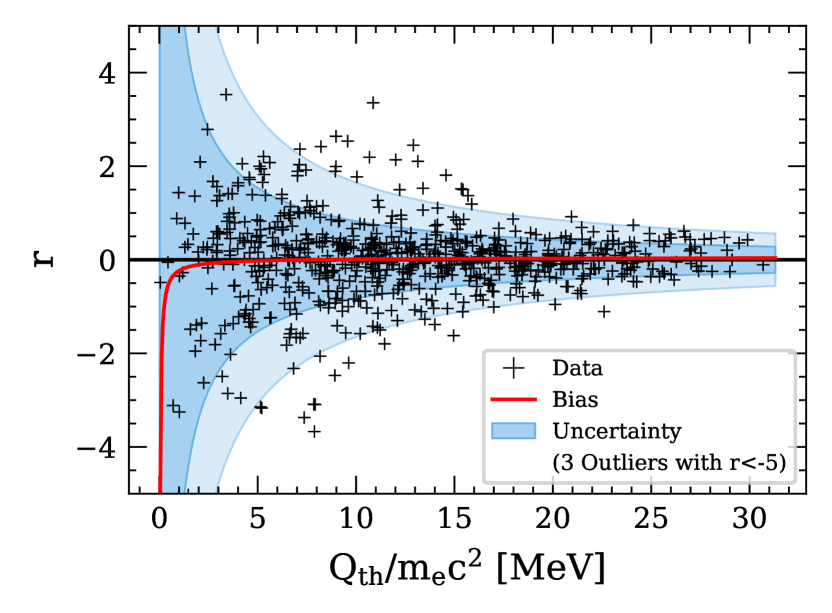
Figure 5: Bayesian fit to the bias function and one- and two-standard-deviation bands.

IV.3 Comparisons

To evaluate our data where experimental values are unavailable, we compare our results to those of other global beta-decay calculations. The authors of Ref. Homma et al. (1996) (labeled “Homma” in Fig. 6) conducted a microscopic pnQRPA calculation with schematic allowed and unique first-forbidden interactions, and treated odd nuclei perturbatively. Reference Nakata et al. (1997) (labeled “Nakata”) carried out a macroscopic calculation within the semi-gross theory. Reference Möller et al. (2003) (labeled Möller) combined microscopic and macroscopic approaches, using the finite-range droplet model for ground state properties, the pnQRPA with an empirical spreading for Gamow-Teller strength, and the gross theory for first-forbidden contributions. More recently, Ref. Costiris et al. (2009) (labeled “Costiris”) applied a neural network to predict half-lives. Finally, Ref. Marketin et al. (2016) (labeled “Marketin”) conducted a fully self-consistent covariant pnQRPA calculation with local fits to the isoscalar pairing strength, treating odd nuclei as if they were fully paired even nuclei with an odd number of nucleons on average.

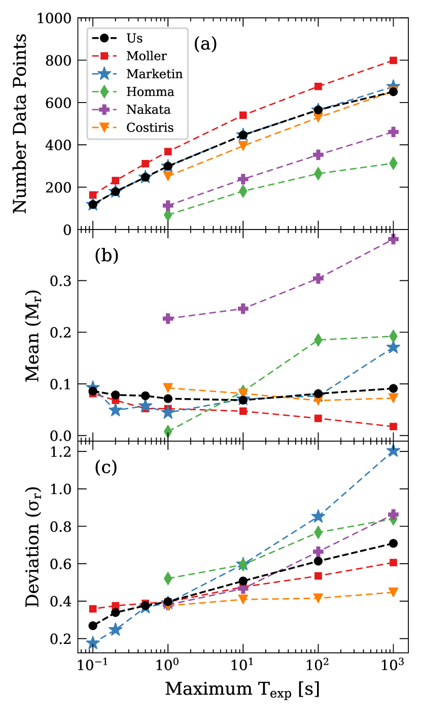
Figure 6: Comparison of error-evaluation parameters among results of Refs. Marketin et al. (2016) (Marketin), Möller et al. (2003) (Möller), Costiris et al. (2009) (Costiris), Nakata et al. (1997) (Nakata), and Homma et al. (1996) (Homma).

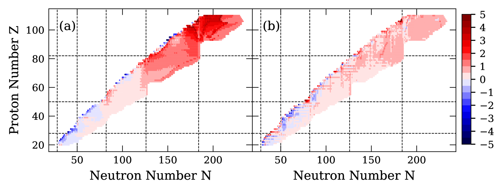
Figure 7: Log of the ratio of our half-lives to those of a) Ref. Marketin et al. (2016) and b) Ref. Möller et al. (2003).

To compare our results to those of the other papers, we use the quality measures outlined, e.g., in Ref. Möller et al. (2003): the mean $(M_{r})$ and standard deviation $(\sigma_{r})$ of the error parameter in Eq. (20),

$$M_{r}=\frac{1}{n}\sum\limits_{i=1}^{n}r_{i},\quad\sigma_{r}=\bigg{[}\frac{1}{n}\sum\limits_{i=1}^{n}(r_{i}-M_{r})^{2}\bigg{]}^{1/2}\,.$$ (29)

We present these measures for the set of nuclei with experimental half-lives less than 1000 s, 100 s, 1 s, 0.5 s, 0.2 s, and 0.1 s. For Refs. Homma et al. (1996); Nakata et al. (1997); Costiris et al. (2009) we take the measures directly from the corresponding paper. References Möller et al. (2003); Marketin et al. (2016) supplied their data set as supplemental material, and we recompute the quality measures with the more recent 2019 ENSDF experimental half-lives Evaluated Nuclear Structure Data File (2019) (ENSDF). Figure 6 summarizes the results. The differences in experimental data sets considered in each paper can be seen in part by noting the number of data points used to compute the quality measures. The errors for Ref. Marketin et al. (2016) are somewhat larger for long-lived isotopes than the values given in that paper because we include all the calculations in odd nuclei, while the authors excluded a few that they considered outliers. In general, our calculation is comparable in fidelity to the others. Unlike those, however, its treatment of odd nuclei is fully self-consistent, capturing in part the one-quasiparticle nature of such states through the EFA, and it uses a single energy functional with no local adjustments. Figure 7 compares all our results with those provided in Refs. Möller et al. (2003); Marketin et al. (2016). We generally predict longer half-lives than the other two models in heavier nuclei, and slightly shorter half-lives in lighter nuclei. The vast majority of our numbers fall within one order of magnitude of those of Ref. Möller et al. (2003). Both we and Ref. Möller et al. (2003) predict significantly longer half-lives in heavy isotopes than does Ref. Marketin et al. (2016). There do not appear to be any other significant systematic differences among the results.

V Conclusions

Using the statistical extension of the charge-changing finite amplitude method, we computed beta-decay half-lives of almost all odd-mass and odd-odd nuclei on the neutron-rich side of stability, in a fully microscopic and self-consistent way. The equal filling approximation allows us to retain time-reversal symmetry while sill largely including the effects of core polarization by the odd nucleon. We showed that in a few cases the EFA leads to the appearance of negative and even imaginary eigenvalues. Overall our half-lives are similar to those of other global calculations in reproducing experimental data. We supplemented these calculations with an estimate of theoretical uncertainties, which suggest that calculated half-lives fall within two orders of magnitude of experimental values for nuclei with $Q$-values greater than about 2 MeV. We also find, as do other groups, that first-forbidden contributions are important in many nuclei. We provided all the half-lives described here, along with associated ground-state properties, error estimates, and Gamow-Teller strength distributions, in the supplemental material sup .

We plan to extend our methods in several ways:

• We will use the statistical FAM with the grand canonical ensemble for finite temperature beta-decay calculations. Decay at non-zero temperature plays an important role in neutron-star mergers and core-collapse supernovae Langanke and Martínez-Pinedo (2000); Langanke et al. (2001).

• We will improve the ability of the FAM to capture low-energy strength by including correlations beyond the QRPA. Although one must be careful in combining such correlations with density functionals, several procedures exist for doing so Gambacurta et al. (2015); Robin and Litvinova (2016); Niu et al. (2018). An efficient implementation of an extension to the FAM would allow better global calculations.

• Finally, we will better treat the weak interaction. Here we restrict ourselves to the impulse approximation, neglecting many-body currents completely. Recent work shows that such currents account for a significant fraction of the quenching of Gamow-Teller strength Gysbers et al. (2019). With an additional extension of the pnFAM we can take two-body currents into account.

Our calculations are also an important milestone in the development of a consistent description of the fission process within nuclear DFT Schunck and Robledo (2016). Although spontaneous fission-fragment half-lives, fragment distributions, and fragment excitation energies can already be computed in DFT, our work paves the way to for a description of the deexcitation of the fragments, including gamma emission and beta decay, within the same framework.

References

- Burbidge et al. (1957) E. M. Burbidge, G. R. Burbidge, W. A. Fowler, and F. Hoyle, Rev. Mod. Phys. 29, 547 (1957).
- Meyer (1994) B. S. Meyer, Annu. Rev. Astron. Astrophys. 32, 153 (1994).
- LIGO Scientific Collaboration and Virgo Collaboration (2017) LIGO Scientific Collaboration and Virgo Collaboration, Phys. Rev. Lett. 119, 161101 (2017).
- Horowitz et al. (2019) C. J. Horowitz, A. Arcones, B. Cote, I. Dillmann, W. Nazarewicz, I. Roederer, H. Schatz, A. Aprahamian, D. Atanasov, A. Bauswein, T. C. Beers, J. Bliss, M. Brodeur, J. Clark, A. Frebel, F. Foucart, C. Hansen, O. Just, A. Kankainen, G. McLaughlin, J. Kelly, S. Liddick, D. Lee, J. Lippuner, D. Martin, J. Mendoza-Temis, B. T. Metzger, M. Mumpower, G. Perdikakis, J. Pereira, B. O’Shea, R. Reifarth, A. Rogers, D. Siegel, A. Spyrou, R. Surman, X.-D. Tang, T. Uesaka, and M. Wang, J. Phys. G: Nucl. Part. Phys. , (2019).
- Evaluated Nuclear Structure Data File (2019) (ENSDF) Evaluated Nuclear Structure Data File (ENSDF), (2019), http://www.nndc.bnl.gov/ensarchivals.
- Möller et al. (1997) P. Möller, J. Nix, and K.-L. Kratz, At. Data Nucl. Data Tables 66, 131 (1997).
- Engel et al. (1999) J. Engel, M. Bender, J. Dobaczewski, W. Nazarewicz, and R. Surman, Phys. Rev. C 60, 014302 (1999).
- Mumpower et al. (2014) M. Mumpower, J. Cass, G. Passucci, R. Surman, and A. Aprahamian, AIP Adv. 4, 041009 (2014).
- Shafer et al. (2016) T. Shafer, J. Engel, C. Frohlich, G. C. McLaughlin, M. Mumpower, and R. Surman, Phys. Rev. C 94, 055802 (2016).
- Nakata et al. (1997) H. Nakata, T. Tachibana, and M. Yamada, Nucl. Phys. A 625, 521 (1997).
- Möller et al. (2003) P. Möller, B. Pfeiffer, and K.-L. Kratz, Phys. Rev. C 67, 055802 (2003).
- Marketin et al. (2016) T. Marketin, L. Huther, and G. Martínez-Pinedo, Phys. Rev. C 93, 025805 (2016).
- Ring and Schuck (2004) P. Ring and P. Schuck, The Nuclear Many-Body Problem (Springer, 2004).
- Schunck (2019) N. Schunck, Energy Density Functional Methods for Atomic Nuclei (IOP Publishing, 2019).
- Bertsch et al. (2009a) G. Bertsch, J. Dobaczewski, W. Nazarewicz, and J. Pei, Phys. Rev. A 79, 043602 (2009a).
- Schunck et al. (2010) N. Schunck, J. Dobaczewski, J. McDonnell, J. Moré, W. Nazarewicz, J. Sarich, and M. V. Stoitsov, Phys. Rev. C 81, 024316 (2010).
- Homma et al. (1996) H. Homma, E. Bender, M. Hirsch, K. Muto, H. V. Klapdor-Kleingrothaus, and T. Oda, Phys. Rev. C 54, 2972 (1996).
- Perez-Martin and Robledo (2008) S. Perez-Martin and L. M. Robledo, Phys. Rev. C 78, 014304 (2008).
- Duguet et al. (2001) T. Duguet, P. Bonche, P.-H. Heenen, and J. Meyer, Phys. Rev. C 65, 014311 (2001).
- Bertsch et al. (2009b) G. F. Bertsch, C. A. Bertulani, W. Nazarewicz, N. Schunck, and M. V. Stoitsov, Phys. Rev. C 79, 034306 (2009b).
- Mustonen and Engel (2016) M. T. Mustonen and J. Engel, Phys. Rev. C 93, 014304 (2016).
- Nakatsukasa et al. (2007) T. Nakatsukasa, T. Inakura, and K. Yabana, Phys. Rev. C 76, 024318 (2007).
- Avogadro and Nakatsukasa (2011) P. Avogadro and T. Nakatsukasa, Phys. Rev. C 84, 014314 (2011).
- Nikšić et al. (2013) T. Nikšić, N. Kralj, T. Tutiš, D. Vretenar, and P. Ring, Phys. Rev. C 88, 044327 (2013).
- Liang et al. (2013) H. Liang, T. Nakatsukasa, Z. Niu, and J. Meng, Phys. Rev. C 87, 54310 (2013).
- Liang et al. (2014) H. Liang, T. Nakatsukasa, Z. Niu, and J. Meng, Phys. Scr. 89, 054018 (2014).
- Inakura et al. (2009a) T. Inakura, T. Nakatsukasa, and K. Yabana, Phys. Rev. C 80, 044301 (2009a).
- Inakura et al. (2009b) T. Inakura, T. Nakatsukasa, and K. Yabana, Eur. Phys. J. A 42, 591 (2009b).
- Inakura et al. (2010) T. Inakura, T. Nakatsukasa, and K. Yabana, Mod. Phys. Lett. A 25, 1931 (2010).
- Stoitsov et al. (2011) M. Stoitsov, M. Kortelainen, T. Nakatsukasa, C. Losa, and W. Nazarewicz, Phys. Rev. C 84, 041305(R) (2011).
- Oishi et al. (2016) T. Oishi, M. Kortelainen, and N. Hinohara, Phys. Rev. C 93, 34329 (2016).
- Mustonen et al. (2014) M. T. Mustonen, T. Shafer, Z. Zenginerler, and J. Engel, Phys. Rev. C 90, 024308 (2014).
- Nakatsukasa (2014) T. Nakatsukasa, J. Phys. Conf. Ser. 533, 012054 (2014).
- Hinohara (2015) N. Hinohara, Phys. Rev. C 92, 34321 (2015).
- Hinohara et al. (2013) N. Hinohara, M. Kortelainen, and W. Nazarewicz, Phys. Rev. C 87, 064309 (2013).
- Hinohara et al. (2015) N. Hinohara, M. Kortelainen, W. Nazarewicz, and E. Olsen, Phys. Rev. C 91, 044323 (2015).
- Sommermann (1983) H. M. Sommermann, Ann. Phys. (N. Y). 151, 163 (1983).
- Goodman (1981) A. L. Goodman, Nucl. Phys. A352, 30 (1981).
- Bohr and Mottelson (1998) A. Bohr and B. R. Mottelson, Nuclear Structure Volume II: Nuclear Deformations (World Scientific, 1998).
- Reinhard et al. (1999) P. G. Reinhard, D. J. Dean, W. Nazarewicz, J. Dobaczewski, J. A. Maruhn, and M. R. Strayer, Phys. Rev. C 60, 014316 (1999).
- Perez et al. (2017) R. N. Perez, N. Schunck, R. D. Lasseri, C. Zhang, and J. Sarich, Comput. Phys. Commun. 220, 363 (2017).
- Runge (1901) C. Runge, Zeitschrift fur Math. und Phys. 46, 224 (1901).
- (43) See Supplemental Material at [URL will be inserted by publisher] for tables of beta decay properties and strength functions.
- Suhonen (2007) J. Suhonen, From Nucleons to Nucleus: Concepts of Microscopic Nuclear Theory (Springer, 2007).
- Bailer-Jones (2017) C. A. L. Bailer-Jones, Practical Bayesian Inference: A Primer for Physical Scientists (Cambridge University Press, 2017).
- Costiris et al. (2009) N. J. Costiris, E. Mavrommatis, K. A. Gernoth, and J. W. Clark, Phys. Rev. C 80, 044332 (2009).
- Langanke and Martínez-Pinedo (2000) K. Langanke and G. Martínez-Pinedo, Nucl. Phys. A 673, 481 (2000).
- Langanke et al. (2001) K. Langanke, E. Kolbe, and D. J. Dean, Phys. Rev. C 63, 032801(R) (2001).
- Gambacurta et al. (2015) D. Gambacurta, M. Grasso, and J. Engel, Phys. Rev. C 92, 034303 (2015).
- Robin and Litvinova (2016) C. Robin and E. Litvinova, Eur. Phys. J. A 52, 205 (2016).
- Niu et al. (2018) Y. F. Niu, Z. M. Niu, G. Colò, and E. Vigezzi, Phys. Lett. B 780, 325 (2018).
- Gysbers et al. (2019) P. Gysbers, G. Hagen, J. D. Holt, G. R. Jansen, T. D. Morris, P. Navrátil, T. Papenbrock, S. Quaglioni, A. Schwenk, S. R. Stroberg, and K. A. Wendt, Nat. Phys. 15, 428 (2019).
- Schunck and Robledo (2016) N. Schunck and L. M. Robledo, Rep. Prog. Phys. 79, 116301 (2016).