Quantum Divide and Compute: Hardware Demonstrations and Noisy Simulations
Abstract
Noisy, intermediate-scale quantum computers come with intrinsic limitations in terms of the number of qubits (circuit “width”) and decoherence time (circuit “depth”) they can have. Here, for the first time, we demonstrate a recently introduced method that breaks a circuit into smaller subcircuits or fragments, and thus makes it possible to run circuits that are either too wide or too deep for a given quantum processor. We investigate the behavior of the method on one of IBM’s 20-qubit superconducting quantum processors with various numbers of qubits and fragments. We build noise models that capture decoherence, readout error, and gate imperfections for this particular processor. We then carry out noisy simulations of the method in order to account for the observed experimental results. We find an agreement within 20% between the experimental and the simulated success probabilities, and we observe that recombining noisy fragments yields overall results that can outperform the results without fragmentation.
Because of rapid technological progress, quantum processors of increasing quality and size are becoming available, whether of the superconducting [1] or of the trapped-ion [2] type. Despite this steady improvement, these noisy, intermediate-scale quantum (NISQ [3]) devices are still limited in both their number of qubits (with, e.g., 53 qubits [4]) and their coherence time. Both constraints prevent one from performing quantum algorithms that require a large number of qubits or operations. Peng et al. [5] recently proposed a method to circumvent this limitation. Basing their method on tensor-network techniques, they showed how to decompose a circuit with a large quantum volume [6] into smaller subcircuits with quantum volumes compatible with NISQ devices.
Here, we show the first practical implementation of this method on an actual 20-qubit quantum device for a Greenberger-Horne-Zeilinger (GHZ) type of test circuit with a qubit count of up to 24 and various fragments sizes. Rather than focusing on large qubit counts, we investigate the extent to which this method can deal with decoherence in smaller circuits through experimental runs and noisy simulation of this decoherence. To this aim, we establish a precise noise model of IBM’s 20-qubit Johannesburg processor using available calibration data, and we use the model to simulate the experimental results. This noisy simulation allows us to quantify and explain the experimental results we obtain, and it paves the way to a noise-aware optimization of this fragmentation technique.
I Methods: circuit fragmentation and noise modeling
I-A Basics of circuit fragmentation
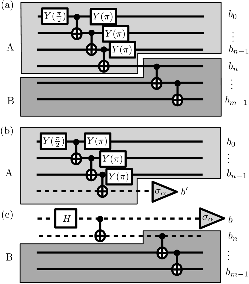
The execution of a quantum circuit on an -qubit quantum computer yields measurements in the form of bitstrings whose probability is given by Born’s rule, , where is the initial state of the quantum register (here ) and is the unitary operation defining the quantum circuit. is composed of a sequence of local unitary operations called quantum gates that can be represented as the vertices of a graph. If the underlying graph can be broken into disconnected components or “fragments” upon removal of edges, the circuit’s probability distribution can be computed from the suitably modified probability distributions of the fragments [5]. For instance, the circuit in Fig. 1(a) is represented by a graph that separates into two disconnected components (light gray [A] and dark gray [B]) when removing a single edge (here on qubit with index between the two CNOT gates). In this configuration, the full probability distribution can be computed as
| (1) | |||
with , and . Here, denotes the probability of measuring the bitstring when measuring the final state of fragment along axis for qubit (Fig. 1(b)), while is the probability of getting bitstring after preparing the first two qubits (the first two qubits of fragment ) in the Bell state and measuring the final state of fragment with the ancilla qubit measured along axis (Fig. 1(c)). This procedure can be repeated recursively to break the circuit into ever smaller fragments.
With this procedure, a wide and deep quantum circuit can be fragmented into smaller circuits that can be run on a NISQ processor. However, doing so comes at a cost, in terms of the number of individual subcircuits to be run, that is exponential in the number of removed edges or “cuts” [5].
In this work, we focus on the GHZ-type circuit shown in Fig. 1(a). The resulting maximally entangled state, , is very sensitive to decoherence and is therefore a good test case for investigating the resilience of the method on noisy processors.
I-B Noise modeling and simulation
To simulate the behavior of the method on noisy processors, we model the processor errors by combining three error sources: decoherence of the amplitude damping and dephasing types during qubit idling (inactive) periods, readout errors, and gate imperfections.
We set the amplitude damping, dephasing, and readout errors using calibration data supplied on the IBM Quantum Experience platform. Averaging over the 20 qubits of the chip, we find , , and a readout error rate of . The and processes are modeled by the combination of the amplitude damping (AD) and pure dephasing (PD) quantum channels defined by the Kraus operators
where is the duration of the idling period during which the noise acts, and , with . To determine the idling durations, we assume the following durations for the gates: 200 ns for the CNOT gate, and 20 ns for the single-qubit gates. As for the readout errors, we choose to model them as a single-qubit relaxation (amplitude damping) process during the measurement time. The corresponding 2-outcome positive-operator valued measure (POVM) has elements , with
where . We check that the measurement duration we infer from the experimental calibration error rate , namely , is consistent with usual values for this duration.
We model the gate imperfections using a simple depolarizing noise channel following each one-qubit gate, with Kraus operators
where denote the Pauli spin matrices. For the two-qubit (CNOT) gates, we use the tensor product of the above depolarizing channel to mimic two-qubit errors after each CNOT gate. We adjust the depolarizing probabilities and to have the error channels match given average process fidelities and (as defined in e.g [7]) or equivalently average errors and (with ). and are themselves fixed using the qubit-averaged calibration error rates supplied by IBM Quantum Experience, and .
We use the obtained Kraus operators to simulate the noisy evolution combined with fragmentation. Prior to the noisy simulation, the circuit is compiled to comply with the target processor’s qubit connectivity graph using the Atos Quantum Learning Machine (QLM)’s dedicated Nnizer plugin. This results in longer circuits owing to the (optimized) insertion of SWAP gates whenever needed. The noisy simulations are carried out on the QLM using density-matrix-based simulations.
II Results
We implemented the circuit fragmentation procedure and tested it on an experimental qubit platform, IBM’s 20-qubit Johannesburg processor, comprising superconducting transmon qubits arranged in a two-dimensional grid. We accessed this processor via the IBM Quantum Experience cloud platform and used the Qiskit programming framework to describe the circuits. As a proxy for the quality of the final result, we calculated the following sum of probabilities
| (2) |
which is unity in the absence of any noise.
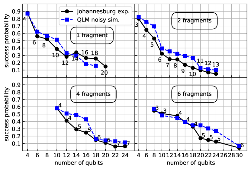
The experimental and noisy simulation results for up to 30 qubits are shown in Fig. 2. This figure includes the statistical error bars (standard error of the mean) on the probabilities after recombination. These errors originate from the finite number of shots (8192) per fragment. We computed them using resampling. Because of the large number of shots, they are comprised within the size of the datapoints and therefore do not appear on the graph.
The one-fragment case (top-left panel), corresponding to running the original circuit without fragmentation, will serve as our reference curve. It displays a marked decrease in the success probability as the number of qubits increases. For all fragment numbers, the values obtained for the success probability obtained experimentally and with noisy simulation agree within 20% (in absolute values). In particular, discontinuities and even some of the sign changes of the slope of are captured by noisy simulations. The drops in success probability in going from a fragment size of 5 to a fragment size of 6 (and similarly 10 to 11 and 15 to 16) are easily accounted for by the topology requirements of the chip (in the absence of qubit relabeling, running a fragment of size 6 will require introducing SWAP gates to perform a CNOT gate between qubits of indices 4 and 5, which are not nearest neighbors on the chip). The noisy simulations tend to overestimate the success probability compared to the experimental results. Uncaptured phenomena such as temporal and spatial (crosstalk) noise likely account for the discrepancy.
Remarkably, both experimental and noisy simulation results show that increasing the number of fragments allows us to reach reasonable success probabilities as the circuit sizes increase: thus, the success rate drop after 4 qubits for the one-fragment case only occurs for circuit sizes of 8 and 16 qubits when breaking the circuit into 2 and 4 fragments, respectively (for the 6-fragment case, the experimental values show a drop after 18 qubits, while the noisy simulation show the same drop after 24 qubits). Thus, the method makes it possible not only to perform computations for circuit sizes exceeding the chip’s size (see, e.g, the runs), but also to obtain better success probabilities for smaller circuit sizes.
Acknowledgment
This research used resources of the Oak Ridge Leadership Computing Facility, which is a DOE Office of Science User Facility supported under Contract DE-AC05-00OR22725. This research also used the resources of the Argonne Leadership Computing Facility, which is DOE Office of Science User Facility supported under Contract DE-AC02-06CH11357. Yuri Alexeev, Zain H. Saleem, and Martin Suchara were supported by the DOE, Office of Science, under Contract DE-AC02-06CH11357. The compilation and noisy simulations were performed using Argonne National Laboratory’s and Atos Quantum Laboratory’s Quantum Learning Machines.
References
- [1] M. Kjaergaard, M. E. Schwartz et al., “Superconducting Qubits: Current State of Play,” Annual Review of Condensed Matter Physics, vol. 11, no. 1, pp. 031 119–050 605, Mar. 2020. [Online]. Available: https://www.annualreviews.org/doi/10.1146/annurev-conmatphys-031119-050605
- [2] C. D. Bruzewicz, J. Chiaverini et al., “Trapped-ion quantum computing: Progress and challenges,” Applied Physics Reviews, vol. 6, no. 2, p. 021314, Jun. 2019. [Online]. Available: http://aip.scitation.org/doi/10.1063/1.5088164
- [3] J. Preskill, “Quantum Computing in the NISQ era and beyond,” Quantum, vol. 2, p. 79, Aug. 2018. [Online]. Available: http://dx.doi.org/10.22331/q-2018-08-06-79
- [4] F. Arute, K. Arya et al., “Quantum supremacy using a programmable superconducting processor,” Nature, vol. 574, no. 7779, pp. 505–510, Oct. 2019. [Online]. Available: http://dx.doi.org/10.1038/s41586-019-1666-5
- [5] T. Peng, A. Harrow et al., “Simulating large quantum circuits on a small quantum computer,” Mar. 2019. [Online]. Available: http://arxiv.org/abs/1904.00102
- [6] A. W. Cross, L. S. Bishop et al., “Validating quantum computers using randomized model circuits,” Physical Review A, vol. 100, no. 3, p. 032328, Sep. 2019. [Online]. Available: http://dx.doi.org/10.1103/PhysRevA.100.032328
- [7] A. Gilchrist, N. K. Langford, and M. A. Nielsen, “Distance measures to compare real and ideal quantum processes,” Physical Review A, vol. 71, no. 6, pp. 1–15, Aug. 2005. [Online]. Available: https://link.aps.org/doi/10.1103/PhysRevA.71.062310