Superfluid and supersolid phases of ⁴He on the second layer of graphite

Abstract

We revisited the phase diagram of the second layer of ⁴He on top of graphite using quantum Monte Carlo methods. Our aim was to explore the existence of the novel phases suggested recently in experimental works, and determine their properties and stability limits. We found evidence of a superfluid quantum phase with hexatic correlations, induced by the corrugation of the first Helium layer, and a quasi-two-dimensional supersolid corresponding to a 7/12 registered phase. The 4/7 commensurate solid was found to be unstable, while the triangular incommensurate crystals, stable at large densities, were normal.

The light mass of Helium atoms and the strong Carbon-Helium interaction make ⁴He adsorbed on graphite the most paradigmatic example of a two-dimensional (2D) quantum system. Its phase diagram was extensively studied in the 90’s, using a variety of experimental techniques (see, for instance, Ref. cole, ). The consensus so far is that, at very low temperature, ⁴He in direct contact with the graphite surface is a $\sqrt{3}\times\sqrt{3}$ registered solid that undergoes a first-order phase transition to a incommensurate triangular 2D crystal upon increasing the Helium density. This was also confirmed by first-principles theoretical descriptions of the system corboz ; yo . Quantum Monte Carlo simulations in the limit of zero temperature found other proposed commensurate phases to be unstable yo .

By increasing the Helium coverage, the system undergoes first-order layering transitions, a feature that was clearly observed recently on a single carbon nanotube adrian . In graphite, there seemed to be a consensus about the second ⁴He layer, stable in the coverage range $\sim$ 0.114-0.200 Å^-2. Those are total densities, including helium atoms per surface unit both in the first and second layers. Heat capacity greywall1 ; greywall and torsional oscillator B7 ; B8 experiments indicated that, after a promotion from the first to the second layer a quasi-two-dimensional liquid was formed. Increasing the coverage, the liquid changes into a commensurate phase (with respect to the first adsorbed Helium layer), and then to an incommensurate one before promotion to a third layer greywall1 ; greywall .

Remarkably, two recent experimental works have reopened the doubts about the phase diagram of the second layer of ⁴He adsorbed on graphite. First, the calorimetric data of Ref. B12, suggests the existence of a liquid above 0.175 Å^-2, followed upon an increasing of the helium coverage, of a stable phase in the 0.196-0.203 Å^-2 range. That phase could be either a commensurate solid or a quantum hexatic phase. On the other hand, the torsional oscillator data of Ref. B13, indicate a normal 2D liquid between $\sim$0.1657 Å^-2 and 0.1711 Å^-2 (Ref. B13, , supplementary information), followed by an arrangement showing a superfluid response from 0.1711 to 0.1996 Å^-2, with a maximum at 0.1809 Å^-2. Since, according to previous DMC calculations B10 , those densities are above the stability limits of a liquid phase, that response would correspond to a quasi-two-dimensional supersolid. This would be the first indication of a stable supersolid phase in ⁴He, after discarding that possibility in bulk chan .

In this Letter, we revisit this problem from a theoretical microscopic point of view. Our aim is to clarify the nature of the stable phases of the second layer of ⁴He on graphite, in the limit of zero temperature. Our results show hexatic order hexatic ; hexatic2 ; hexatic3 before crystallization into one of the possible registered phases (7/12). In both cases, our measure of the superfluid fraction gives a finite value, larger for the hexatic but still very significant for the registered solid. Therefore, on this layer we found two long pursued phases: a superhexatic superhexatic and a quasi-two dimensional (registered) supersolid.

Our zero-temperature first-principles study relies on the diffusion Monte Carlo (DMC) method, used extensively in the past to analyze ⁴He phases in different geometries borobook . The high numerical accuracy of DMC in the estimation of the energy is crucial to disentangle the stability of different possible phases. This is specially relevant in the study of registered phases since the energy differences between different commensurate solids is very tiny. In essence, the DMC method allows us to solve the many-body imaginary-time Schrödinger equation corresponding to the Hamiltonian describing the system boro94 . In the present case,

$$H=\sum_{i=1}^{N}\left[-\frac{\hbar^{2}}{2m}\nabla_{i}^{2}+V_{{\rm ext}}(x_{i},y_{i},z_{i})\right]+\sum_{i<j}^{N}V_{\rm{He-He}}(r_{ij})\ ,$$ (1)

where $x_{i}$, $y_{i}$, and $z_{i}$ are the coordinates of the $N$ Helium atoms, including first and second layers, and $m$ is the ⁴He mass. Graphite was modeled by a set of eight graphene layers separated $3.35$ Å in the $z$ direction and stacked in the A-B-A-B way typical of this compound, as in Ref. yo, . We stopped at eight graphene sheets since to include a ninth one changes the energy per particle less than the typical error bars for that magnitude (around 0.1 K) yo . $V_{{\rm ext}}(x_{i},y_{i},z_{i})$ sums, for each ⁴He atom $i$, all the C-He pair interactions calculated using the accurate Carlos and Cole anisotropic potential carlosandcole . The He-He interaction $V_{{\rm He-He}}(r_{ij})$ is modeled using a standard Aziz potential aziz . The graphite substrate was considered to be rigid, but the helium atoms in both the first and second layers were allowed to move from their crystallographic positions.

In order to reduce the variance and to fix the phase under study, DMC incorporates importance sampling by using a guiding wave function. This wave function is designed as a first, simple approximation to the many-body system and is variationally optimized. In our case, we used

$$\Phi({\bf r}_{1},\ldots,{\bf r}_{N}) = \Phi_{J}({\bf r}_{1},\ldots,{\bf r}_{N})\Phi_{1}({\bf r}_{1},\ldots,{\bf r}_{N_{1}})$$ (2)

$$\times\ \Phi_{2}({\bf r}_{N_{1}+1},\ldots,{\bf r}_{N})\ ,$$

with

$$\Phi_{J}({\bf r}_{1},\ldots,{\bf r}_{N})=\prod_{i<j}^{N}\exp\left[-\frac{1}{2}\left(\frac{b}{r_{ij}}\right)^{5}\right]\$$ (3)

a Bijl-Jastrow wave function built as a product of McMillan pair correlation factors with a variational parameter $b$, whose value was taken from the literature boro94 ; yo . The one-body terms of the $N_{1}$ atoms in the first layer (2) are given by

$$\Phi_{1}({\bf r}_{1},\ldots,{\bf r}_{N_{1}})=\prod_{i=1}^{N_{1}}\Psi_{1}(z_{i})$$ (4)

$$\times\prod_{i,I=1}^{N_{1}}\exp\{-a_{1}[(x_{i}-x_{I}^{(1)})^{2}+(y_{i}-y_{I}^{(1)})^{2}]\}\ .$$

Following Ref. yo, , $\Psi_{1}(z_{i})$ is the solution to the one-body Schrödinger equation that describes a single Helium atom in a z-averaged helium-graphite potential, $a_{1}$ being a variational parameter different for each ⁴He first layer density. The coordinate set $(x_{I}^{(1)},y_{I}^{(1)})$ corresponds to the $N_{1}$ crystallographic sites of that first layer. On the other hand, the second layer was described by a symmetric Nosanow function to allow for possible exchanges in the crystal yo3 ,

$$\Phi_{2}({\bf r}_{N+1},\ldots,{\bf r}_{N})=\prod_{i=1}^{N_{1}}\Psi_{2}(z_{i})$$ (5)

$$\times\prod_{i,I=1}^{N_{2}}\left[\sum_{i=N_{1}+1}^{N}\exp\{-a_{2}[(x_{i}-x_{I}^{(2)})^{2}+(y_{i}-y_{I}^{(2)})^{2}]\}\ \right],$$

Here, $\Psi_{2}(z_{i})$ is a Gaussian of the type $\exp[-c_{2}(z_{i}-z_{m})^{2}]$, with both $c_{2}$ and $z_{m}$ variationally optimized parameters. $N_{2}$ stands both for the number of Helium atoms on the second layer and for the number of lattice points of the solids. Therefore, no vacancies were considered in any solid. $a_{2}$ was chosen to minimize the total energy of the system. Notice that Eq. (5) can describe a translationally invariant Helium second layer by fixing $a_{2}$ to zero. In most cases, $N_{1}$ was fixed to 224 atoms, distributed in a simulation box including $14\times 8$ triangular unit cells, while $N_{2}$ was fixed to produce the desired density. This meant simulation cells including up to 356 ⁴He atoms.

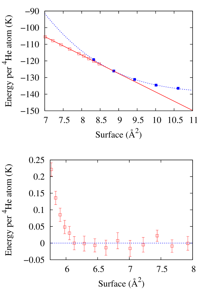
Figure 1: Top panel: Full squares: Energy per ⁴He atom in a single layer of a triangular solid as a function of surface per helium atom. Open squares: Same for an arrangement comprising two helium layers, the density of the first one being 0.115 Å^-2. A least-squares fitting polynomial to the first layer data and the Maxwell construction line between the two arrangements are also shown. Bottom panel: Data for the energy of the second layer system after subtracting the values given by the Maxwell construction line.

Calculating the energy per particle as a function of density, one can establish the stability range of the different phases. The DMC energies are shown in Figs. 1 and 2 for different values of the surface area (the inverse of the surface density). The first issue to be addressed is the determination the first-layer solid density which produces the lowest total energy for a two-layer arrangement. To this end, we followed a procedure used previously for graphene B10 . As in that work, the optimum density of the first layer turned out to be 0.115 Å^-2. A standard Maxwell construction between a system with a single Helium monolayer and a double-layered one with that solid density (Fig. 1, top panel) and a translational invariant second layer, gives us a promotion density of 0.113 $\pm$ 0.002 Å^-2 (corresponding to 8.86 $\pm$ 0.15 Ų). This is similar to the experimental value 0.114 Å^-2 reported in Ref. B13, and somewhat smaller than the other experimental measure, 0.118 Å^-2, that of Ref. B12, . To calculate the lowest density limit for the bilayer arrangement, we subtracted the energy values for the Maxwell construction line from the direct simulation results. The results obtained are shown in the bottom panel of Fig. 1. As one can see, this limiting value is 6.13 $\pm$ 0.15 Ų, which corresponds to a density $\sigma=0.163\pm 0.002$ Å^-2.

A similar procedure allows us to establish the stability limits for larger values of the total ⁴He density. The results are depicted in Fig. 2. There, we can see the energy per atom for different phases. For total density values smaller than 0.185 Å^-2, the underlying Helium density was, as before, 0.115 Å^-2, while for that value up, the energy was lowered by slightly compressing the first layer to a density 0.1175 Å^-2. In Fig. 2, the open circles correspond to the same translationally invariant double layer arrangement already discussed (Fig. 1). The full squares correspond to a bilayer comprising two incommensurate triangular solid layers. The 4/7 and 7/12 commensurate phases with the triangular lattice of the first layer were also considered by an appropriate choice of the set of crystallographic positions defining them. The fact that, in the figure, there are two points for each of those arrangements is due to the fact that we considered the two possibilities for the first-layer densities discussed above. In any case, it is clear from Fig. 2, that the 4/7 arrangement is unstable. On the other hand, the 7/12 phase is right on top of the Maxwell construction line between the translationally-invariant phase and the double triangular solid one. This means we would have a first order phase transition between a translationally-invariant phase of density $\sigma=0.170\pm 0.002$ Å^-2, and a 7/12 registered solid of 0.182 Å^-2. The first layer of this arrangement would be then compressed up to $\sigma=0.186$ Å^-2, that is again in equilibrium with a triangular solid of density 0.188 Å^-2. This is similar to what happens in a ³He double layer system on graphite yo5 , where both the 4/7 and 7/12 phases are stable.

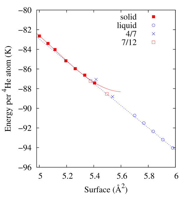
Figure 2: Same than in the previous figure for the two layer system at higher densities. Data for different phases are displayed.

To better characterize the different stable phases, we need to go further than to establish their stability limits. As indicated above, one of the issues raised in Ref. B13, was the possible existence of a quasi-two-dimensional supersolid and of a normal (non superfluid) liquid phase at smaller densities. In order to study those claims, we estimated the superfluid fraction $\sigma_{s}/\sigma$ on the second layer of the arrangements found to be stable. This is done by using the usual winding-number estimator in the limit of zero temperature yo3 ; gubernatis ,

$$\frac{\sigma_{s}}{\sigma}=\lim_{\tau\rightarrow\infty}\alpha\left(\frac{D_{s}(\tau)}{\tau}\right)\ ,$$ (6)

with $\tau$ the imaginary time in the Monte Carlo simulation. Here, $\alpha=N_{2}/(4D_{0})$, $D_{0}=\hbar^{2}/(2m)$, and $D_{s}(\tau)=\langle[{\bf R}_{CM}(\tau)-{\bf R}_{CM}(0)]^{2}\rangle$. ${\bf R}_{CM}$ is the position of the center of mass of the $N_{2}$ ⁴He atoms on the second layer, taking into account only their $x$ and $y$ coordinates (where periodic boundary conditions apply). The results obtained for different cases are shown in Fig. 3. The error bars in that figure correspond to one standard deviation computed from several independent Monte Carlo runs, and when not displayed, are similar to those shown.

In Fig. 3, we see that the translationally invariant phase akin to a liquid found at low densities is a perfect superfluid, since the values for the superfluid estimator are on top to the line corresponding to $\sigma_{s}/\sigma=1$. On the other hand, the superfluid estimator for a triangular solid of $\sigma=0.196$ Å^-2 is zero within our numerical resolution . This situation is common to all other triangular lattice solids, irrespective of their total density, and makes them normal solids. However, the superfluid fraction corresponding to a 7/12 structure with $\sigma=0.186$ Å^-2 (open squares) has an intermediate value between zero and one, corresponding to a superfluid fraction of $0.3\pm 0.1$. This fraction is the same as the one for a $\sigma=0.182$ Å^-2 solid, whose data are not shown for simplicity. This means there is a supersolid stable phase in the density range 0.182-0.186Å^-2. Our results also support the existence of superfluidity in the range between 0.170 and 0.182 Å^-2, in which there is a mixture of a full superfluid liquid-like phase in coexistence with the 7/12 registered solid with the lowest density. The same can be said of the 0.186-0.188Å^-2 interval, where the coexistence is with a normal triangular 2D-solid.

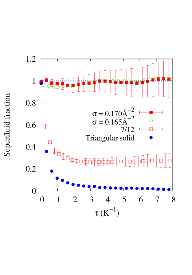
Figure 3: Superfluid density for different second layer arrangements. Full squares, a translationally-invariant phase with $\sigma=0.170$ Å^-2. Open circles, same but for $\sigma=0.165$ Å^-2. Open squares, results for a 7/12 phase with $\sigma=0.186$ Å^-2. Full circles, same for a triangular solid with $\rho=0.196$ Å^-2. The dotted line corresponds to a perfect superfluid with no normal component.

Previous studies on similar systems have always assumed the translationally-invariant phase to be an homogeneous liquid. In this work, we have checked that assumption by considering the possibility of the second layer being some kind of hexatic phase, as suggested in Ref. B12, . To study if this was so, and following Ref. apaja, , we write the pair distribution function $g(r)$ as

$$g(r)=\sum_{n=0}^{\infty}g_{n}(r)\cos(n\theta)$$ (7)

with $n$ even and $\theta={\bf r}\cdot{\bf e}_{0}$. Here, ${\bf e}_{0}$ is a unit vector in a reference direction. The hexatic order in a non-solid phase is associated to a periodic oscillation in the $g_{6}(r)$ component with algebraic decay at large distances hexatic ; hexatic2 ; hexatic3 ; apaja . This hexatic order parameter is shown in Fig. 4 for two translational invariant structures within the stability range of that phase. It is important to stress that the guiding wave function used in DMC to describe those arrangements, a product of Eqs. (3), (4) and (5), this last one with $a_{2}=0$, does not include any explicit hexatic correlation. What we see is a regular pattern of maxima and minima extending to long distances with a slow decay that we cannot determine completely due to the finite size of our simulation box. This ordering is similar to the one found to be metastable in strictly 2D ⁴He at larger densities ($\sigma>0.060$ Å^-2) apaja that the second-layer ones for the systems under consideration (0.047 and 0.055 Å^-2). This fact suggests it to be a consequence of the corrugation of the first layer solid substrate. This underlying structure supports a series of potential minima between every three Helium atoms with the right symmetry to produce the observed order. To check if this is so, we calculated the same parameter for a structure in which the potential created by the second layer had been averaged over to make those potential minima disappear. The result is that the set of maxima and minima are not longer present, indicating that the hexatic correlations are indeed corrugation-induced.

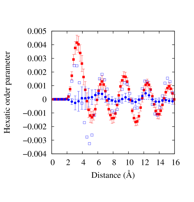
Figure 4: Hexatic order parameter for translationally invariant phases of $\sigma=0.170$ Å^-2 (full squares) and $\sigma=0.163$ Å^-2 (open squares). Full circles correspond to a phase with $\sigma=0.165$ Å^-2, but in which the effect of the first solid layer have been smoothed out. When not displayed, the error bars are similar to the ones shown.

Our theoretical results are at least qualitatively compatible with the available experimental data. For instance, both Refs. B12, and B13, suggest that the phase diagram of the second layer of ⁴He on graphite starts right after promotion with a gas-liquid coexistence zone, followed upon an increase of Helium density to a stable liquid-like region. This would be, at least for the lowest densities ($\sigma<0.170$ Å^-2), a normal fluid that would undergo a first-order phase transition to a commensurate phase. This last phase would change to a high-density triangular solid. Ref. B13, assigns a density range of 0.1711-0.1809 Å^-2 to the liquid-commensurate transition, and of 0.1809-0.1841 Å^-2 for the stable registered phase. Both of them are comparable with our suggestions: 0.170-0.182 Å^-2 and 0.182-0.186 Å^-2, while the data of Ref. B12, is shifted further up in the density scale. In that entire range, we see a superfluid response, first in the coexistence between the superhexatic superhexatic phase and the 7/12 registered solid, and then in the stability range of that phase itself, in accordance with the experimental data of both Refs. B8, and B13, . On the other hand, previous DMC calculations on graphene found the 7/12 commensurate solid to be unstable B10 . This difference in the behavior of those close related systems can be due to the delicate energy balance needed for that structure to be seen: the introduction of the exchanges in the description of the supersolid decreases the energy enough for this commensurate phase to emerge at $T=0$ K. The effect of the additional carbon layers might also play a role, as in the case of the first-layer $\sqrt{3}\times\sqrt{3}$ phase, which is more stable with respect to the metastable liquid in graphite than in graphene yo . On the other hand, the fact that we do see a superfluid response in the range 0.163-0.170 Å^-2 instead of the normal fluid found experimentally, can be due to the lack of connectivity of the real substrate B8 . Finally, the lack of that response beyond 0.188 Å^-2, is in agreement with the results of Ref. B8, .

Our work is carried out strictly at zero temperature and compares very well with recent experiments performed in the mK regime. It would be very interesting to study the same system at finite temperature to determine the thermal stability of the superhexatic and supersolid phases, even though those phases could be unstable at temperature values too low to be accessible to the path integral Monte Carlo method corboz .

- (1) L.W. Bruch,M.W. Cole and E. Zaremba. Physical Adsorption, Forces and Phenomena Dover, New York (1997).
- (2) P. Corboz, M. Boninsegni, L. Pollet, and M. Troyer, Phys. Rev. B 78, 245414 (2008).
- (3) M.C. Gordillo and J. Boronat, Phys. Rev. Lett. 102, 085303 (2009).
- (4) A. Noury, J. Vergara-Cruz, P. Morfin, B. Placais, M. C. Gordillo, J. Boronat, S. Balibar, and A. Bachtold, Phys. Rev. Lett 122, 165301 (2019).
- (5) D.S. Greywall and P.A. Busch. Phys. Rev. Lett 67 3535 (1991).
- (6) D.S. Greywall, Phys. Rev. B 47 309 (1993).
- (7) P. A. Crowell and J. D. Reppy, Phys. Rev. Lett. 70, 3291 (1993).
- (8) P. A. Crowell and J. D. Reppy, Phys. Rev. B 53, 2701 (1996).
- (9) S. Nakamura, K. Matsui, T. Matsui and H. Fukuyama. Phys. Rev. B 94, 180501(R) (2016)
- (10) J. Nyéki, A. Phillis, A. Ho, D. Lee, P. Coleman, J. Parpia, B. Cowan and J. Saunders. Nat. Phys. 13 455 (2017).
- (11) M.C. Gordillo and J. Boronat, Phys. Rev. B, 85 195457 (2012).
- (12) D. Y. Kim and M. H. W. Chan, Phys. Rev. Lett. 109, 155301 (2012).
- (13) B. I. Halperin and D. R. Nelson, Phys. Rev. Lett. 41, 121 (1978).
- (14) D. R. Nelson and B. I. Halperin, Phys. Rev B 19, 2457 (1979).
- (15) A. P. Young, Phys. Rev. B 19, 1855 (1979).
- (16) K. Mullen, H. T. C. Stoof, M. Wallin, and S. M. Girvin, Phys. Rev. Lett. 72, 4013 (1994).
- (17) J. Boronat, in Microscopic Approaches to Quantum Liquids in Confined Geometries, Vol. 4, ed. E. Krotscheck and J. Navarro (World Scientific, Singapore, 2002).
- (18) M.C. Gordillo and J. Boronat. Phys, Rev. Lett. 116 145301 (2016).
- (19) W. E. Carlos and M. W. Cole, Surf. Sci. 91, 339 (1980).
- (20) R.A. Aziz, F.R.W McCourt and C.C. K. Wong. Mol. Phys. 61 1487 (1987).
- (21) J. Boronat and J. Casulleras, Phys. Rev. B 49, 8920 (1994).
- (22) M.C. Gordillo, C. Cazorla, and J. Boronat. Phys. Rev. B 83 121406(R) (2011).
- (23) M.C. Gordillo and J. Boronat. Phys. Rev. B 97 201410(R) (2018).
- (24) S. Zhang, N. Kawashima, J. Carlson and J.E. Gubernatis. Phys. Rev. Lett. 74 1500 (1995).
- (25) V. Apaja and M. Saarela, Europhys. Lett. 84, 40003 (2008).