Just-in-time Quantum Circuit Transpilation Reduces Noise

Abstract

Running quantum programs is fraught with challenges on on today’s noisy intermediate scale quantum (NISQ) devices. Many of these challenges originate from the error characteristics that stem from rapid decoherence and noise during measurement, qubit connections, crosstalk, the qubits themselves, and transformations of qubit state via gates. Not only are qubits not “created equal”, but their noise level also changes over time. IBM is said to calibrate their quantum systems once per day and reports noise levels (errors) at the time of such calibration. This information is subsequently used to map circuits to higher quality qubits and connections up to the next calibration point.

This work provides evidence that there is room for improvement over this daily calibration cycle. It contributes a technique to measure noise levels (errors) related to qubits immediately before executing one or more sensitive circuits and shows that just-in-time noise measurements benefit late physical qubit mappings. With this just-in-time recalibrated transpilation, the fidelity of results is improved over IBM’s default mappings, which only uses their daily calibrations. The framework assess two major sources of noise, namely readout errors (measurement errors) and two-qubit gate/connection errors. Experiments indicate that the accuracy of circuit results improves by 3-304% on average and up to 400% with on-the-fly circuit mappings based on error measurements just prior to application execution.

I Introduction

Today’s quantum computing devices and those of the foreseeable future are referred to as Noisy Intermediate Scale Quantum (NISQ) computers due to the noise inherent in the systems and the small number of quantum bits (qubits) available for calculations [1]. Even when calculations can be performed with a small number of qubits, the noise in the quantum systems frequently produces incorrect results, which presents a challenge in using quantum computation. Consequently, techniques to identify, mitigate, and tolerate noise and even errors in calculations are of considerable importance for quantum computation amid this noisy reality.

Different types of errors can be distinguished. The most commonly reported errors are:

• Readout errors: These are errors in interpreting the state of the qubit at the end of the calculation, e.g., reading a qubit in the $\ket{0}$ state as being in the $\ket{1}$ state.

• Single qubit gate errors: These occur when applying gates to a single qubit causes small changes in the qubit state, which can accumulate over deep circuits with long sequences of gates.

• Two-qubit gate errors: These result from interaction between two qubits under a two-qubit gate operation (e.g., both qubits of a CNOT gate);

• Decoherence errors: These are due to the decay of state over time in today’s quantum devices, and they are referred to as T1, T2, and T2* — but are not addressed in this work.

• Cross-talk errors: These result when the state of a qubit or a resonator between qubits influences the state of another qubit or resonator in close vicinity — but are again beyond the scope of this work.

Each of these errors can vary from one qubit to another and also from one connection (coupling) to another; some qubits/connections experience less noise and fewer errors than others. To make matters more complicated, the qubits themselves change over time in an unpredictable fashion (due to the quantum nature of the qubit system), leading to a need to re-calibrate the qubits and recalculate these errors, e.g., once per day on IBM Q systems.

One way to reduce errors in quantum computations, especially on systems with more physical qubits than necessary for the circuit in question, is to try to map the circuit onto the most appropriate qubits during a process called “transpilation”. Transpilation traditionally considers the mapping of logical qubits in a program onto a physical NISQ device with limited qubit connectivity and native gate operations. This may require a high-level gate (e.g., X/Y/Z rotation) to be translated into one or more low-level gates (e.g., U1/U2/U3 for IBM) with specific phase angles. Transpilation may result in logical qubits being moved (via swap operations) from one physical qubit to another throughout a circuit during its execution. More contemporary transpilation considers virtual-to-physical mappings to the highest fidelity qubits and connection between qubits to reduce the overall error [2, 1]. These optimizations are clearly non-trivial, as many mappings exist in this multi-dimensional non-linear optimization space. For example, the highest fidelity qubits for one circuit may not provide the connections for two-qubit gates of another circuit. It is therefore important to have accurate fidelity data of the physical machine for which a circuit is being transpiled. Different transpilers exist, each of which accept different types of statistical error values per qubit and per coupling between qubits before attempting to provide a high quality mapping. For IBM’s quantum computers, these error metrics are derived from calibration runs of circuits that measure qubits and compare values with reference results. Such calibration occurs usually once per day, and error metrics are published on IBM’s websites and can also be obtained from the Qiskit API [3] for the latest calibration run.

We have performed a series of experiments that, after an initial stable phase, uncovered a quick deterioration in fidelity of qubit gates, measurements and couplings not too long after calibration. These experiments included micro-benchmarks to (a) prepare an $n$ qubit circuit with initial state $\ket{0}^{n}$ followed by simply measuring each qubit and (b) subjecting each qubit to a series of X (NOT) gates before measurement. When repeated hourly, no clear trend became visible. Neither could we detect when the original calibration took place, nor did we observe a gradual de-calibration. When employing longer and more complex circuits and directly comparing different error values, we found that while some qubits remained stable, other qubits showed significant variations in fidelity throughout the day.

These findings motivated us to experiment with obtaining calibration data ourselves, use them in just-in-time transpilation, and then observe errors for this transpiled circuit compared to one transpiled with IBM’s calibration data. Clearly, if virtual-to-physical mappings differ between just-in-time transpilation vs. default transpilation, the fidelity of results can be expected to differ as well.

We chose to focus the investigation on readout errors and two-qubit gate errors in particular, the most significant errors in magnitude. This is also motivated by readout errors affecting every circuit and two-qubit gate errors consistently being about an order of magnitude higher than single qubit gate errors, i.e., the qubit placement of two-qubit gates during transpilation is of high importance for overall fidelity.

Readout errors were determined by immediately measuring a newly prepared qubit and subsequently applying a single X (NOT) gate before measuring the same qubit again. We compared the results to the expected values (of all $\ket{0}$ or all $\ket{1}$, respectively) to obtain the percent error. Two-qubit gate errors were determined by utilizing IBM’s built-in randomized benchmarking capability to obtain an error value. We then subjected transpilation to our error values instead of the default IBM ones (from daily calibration). This resulted in different qubit mappings leading to an improvement of 3-304% on average, and up to 400%.

II Design

The design of our just-in-time transpilation was driven by an initial experiment followed by a methodology to address shortcomings of the current system. While observations are specific to IBM Q devices, the methodological approach is more generic and may transfer to other NISQ devices.

II-A Motivating Experiments

Our first objective was to determine whether or not the fidelity of qubits varied significantly throughout the day. If the fidelity of qubits did not vary significantly between two calibration instances, any effort to repeatedly assess the error rates would likely not contribute to fidelity improvements. To test our hypothesis of variations, we conducted experiments with a number of circuits assessing reported errors throughout the day.

The main focus centered on the qualitative aspect of qubit change, i.e., do qubits provide different results in fidelity over time between calibrations, rather than absolute errors. To this end, experiments were limited to simple circuits to assess readout errors or errors due to successive Pauli gates, which were repeated every hour.

The first experiment focused on readout errors without any gates, where a qubit was initialized ($\ket{0}$ state) and then immediately measured. The second experiment assessed readouts for a qubit after a Pauli X (NOT) gate., i.e., the $\ket{1}$ state. Fig. 1 depicts hourly measurements (x-axis) over the percentage of correct results (y-axis) on different days (colored data series) in 2019 on the IBM Poughkeepsie device (20 qubits). The results show that qubits do not remain stable between calibrations. This behavior was observed across qubits and different IBM Q devices.

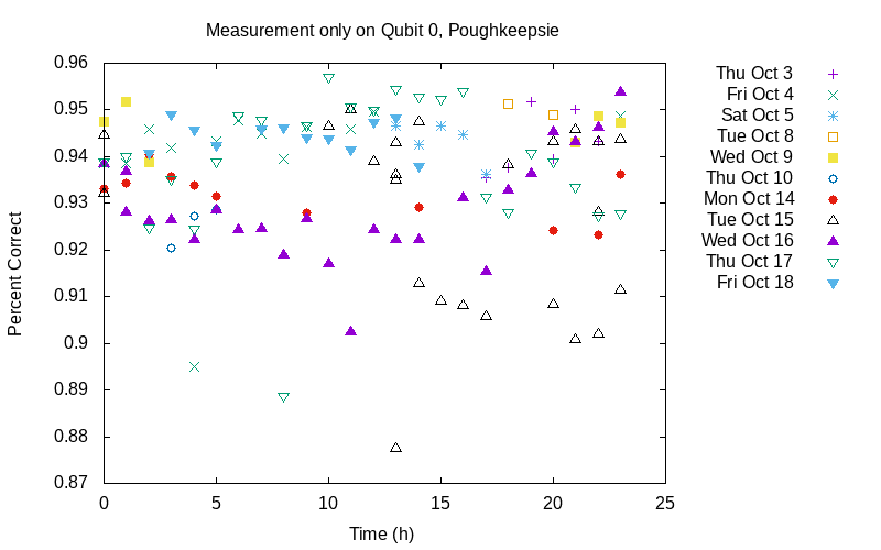
Figure 1: Measurements with no gates on qubit 0 of IBM Poughkeepsie over time. The fidelity of readouts for the qubit varies in a chaotic (non-predictable) manner. Results for other qubits and $\ket{1}$ circuits are similar, figures omitted due to space.

While readout results of these circuits usually did not change drastically from hour to hour, they did change in an unpredictable manner, sometimes resulting in better accuracy, sometimes in worse. This made it impossible to infer or reverse engineer when the calibration actually took place, i.e, we did not observe a drastic change in quality for qubits when measured. We also tested circuits with many gates in a less rigorous manner and observed similar results. Based on prior work, we know that circuits with virtual qubits were mapped onto physical ones via transpilation (at optimization level 3) taking IBM’s error data from the last calibration into account [1, 2]. This led us to the new hypothesis that, when selecting physical qubits to which circuits are to be mapped, a new set of error measurements for just-in-time transpilation might improve the overall fidelity.

II-B Error Selection

A number of different types of errors are taken into account when mapping circuits to qubits, where some of these errors are more prevalent than others as indicated by the respective error metrics. For example, T1 and T2 errors are significant in long circuits but not in short ones. Gate errors will be present in all circuits, but more so in long circuits using many gates. Readout errors need to be taken into account in all circuits. If some errors are more significant than others, those errors dominate the mapping decisions, while other, less significant ones will only marginally contribute.

We decided to focus on two types of errors, those from readouts and those from two-qubit gates. Readout errors affect any circuit, and their probability is relatively high on today’s NISQ computers. Readout errors are reported to be in the order of $10^{-2}$ for IBM Q devices. We even observed that sometimes they can be as high as 10%.

We also focus on two-qubit gate errors for the same reason: They have an equally high error rate (both reported by IBM and observed by us). In contrast, single-qubit gate errors are reported to be lower ($10^{-3}$ for IBM Q devices), and they were also an order of magnitude smaller than readout or two-qubit errors in our experiments.

II-C Methodological Error Collection

The challenge at hand is to reliably collect error characteristics of a physical quantum device that can subsequently be used to map circuits to physical qubits such that overall fidelity can be increased. Readout errors are the easiest to be measured, simply by constructing a circuit that minimizes any of the other types of errors while producing a known measurement value. To minimize gate and time-based errors, the qubits are measured as quickly as possible and with the fewest number of gates. We observe that reading $\ket{0}$ and $\ket{1}$ states each have different error rates [4, 5]. Hence, we utilize two circuits per qubit to characterize readout errors. The first circuit prepares a qubit in the $\ket{0}$ state (as quickly as possible) and measures it, while the second one prepares the qubit in the $\ket{1}$ state via a single X (NOT) gate before measuring.

Gate errors present more of a challenge to be assessed. Recall that we focus on two-qubit gates here due to their higher error rates compared to single qubit gates. Two-qubit gate errors are determined for each pair of connected qubits that can be captured through randomized benchmarking, which uses randomized sequences of gates of increasing length resulting in a known $\ket{0}$ state on qubits. By comparing actual measurements to this known value, error rates are determined. This is described in more detail in [6].

These error characteristics are subsequently used for just-in-time transpilation of circuits for mapping to physical qubits with high fidelity for couplings/connections within the circuit and high measurement quality of selected qubits.

III Implementation

We decided to implement our high-level design of just-in-time transpilation for IBM Q devices using Qiskit. This involves data collection on errors on an IBM Q device, subsequent transpilation of benchmarks via Qiskit at an optimization level that takes errors into account when mapping to physical qubits, and running these benchmarks on the same IBM Q device.

In order to test whether just-in-time error measurement improves performance over using the daily calibrations, we need to to reliably collect data on errors and, for a fair comparison, in a similar manner to how IBM collects data and reports errors during their daily calibrations.

Due to the nature of IBM’s qubits (and other technologies as well), the error for reading a qubit in the $\ket{0}$ ground state state is much lower than reading a qubit in the $\ket{1}$ excited state, which is less stable [4, 5]. IBM determines readout error rates for each state as well as the average of both, which it reports as the readout error. These errors are relatively easily obtained. As described in our motivating experiments, to assess errors for readouts of the $\ket{0}$ state one merely needs to measure immediately after preparing a qubit. Similarly, the $\ket{1}$ state is read out after a qubit is prepared and subjected to a single X (NOT) gate. The observed level of error between the single qubit gate and the readout error, especially when in the $\ket{1}$ state, shows that the contribution of the X gate to the error is negligible (about an order of magnitude lower than the readout error). The readout error is this calculated as the percent of incorrect results returned from the respective circuits.

The two-qubit error requires more complex circuits. We employ Qiskit’s randomized benchmarking capabilities, which can automate the process of data collection. These randomized benchmarks consist of circuits with two qubits that are generated such that their output is an “Error per Clifford” value, which is proportional to the two-qubit error itself.

Obtaining these error metrics for each qubit is a computationally intensive task. Due to limited compute cycles, we decided to combine many of the individual qubit measurements into a single multi-qubit measurement. While this ignores the impact of qubit crosstalk, it still remains useful as any circuit, including our benchmarks, also utilizes multiple qubits, often in close physical vicinity to reduce the number of swaps in transpiled programs. We split the two-qubit gate errors up such that only one coupler of a given qubit was assessed in terms of error at a time. On the IBM Q devices used here, the maximum degree of a qubit is three, i.e., we ran a total of three jobs to capture all two-qubit errors. Once each of these errors had been measured, we assessed the virtual-to-physical mappings. This allowed us to report errors for each physical qubit.

As we are focusing on IBM Q devices, we decided to leverage Qiskit’s built in transpiler using the highest optimization level available (level 3). When compiling benchmarks (or other application programs), this level-3 transpilation triggers an optimization for virtual-to-physical mappings [1].

IV Experimental Setup

We conducted experiments on various IBM Q devices throughout different days and different times as well as repeatedly during a particular day. In every experiment, we first manually measured the CNOT and readout errors and then, based on this error information, transpiled our circuits before sending them to the devices to execute them. We kept track of the circuit layouts post-transpilation and their performance with respect to accuracy. Next, we describe the individual aspects of this setup.

IV-A Device Information

We performed our experiments primarily on two IBM Q devices, Almaden (20 qubits) and Paris (27 qubits). The rationale was to select backends with a sufficient number of possible virtual-to-physical qubit mappings so that the transpilation procedure could adapt mappings to error data. Both devices allow a total of 900 circuits to be sent in one job. Availability of these devices presents another challenge, as they tend to be busy with many jobs in the queue, which meant that the calibration job was running an hour or more before the benchmark jobs as the latter can only be submitted after transpilation taking errors from the former job into account. This assesses just-in-time transpilation in a normal user scenario with so-called “fairshare” queuing. In addition, we conducted experiments in “dedicated” mode, available only to select users, where calibration and benchmark jobs can be run within minutes of each other, again after transpilation of benchmarks based on error data from immediately preceding calibration. Figure 2 depicts the physical qubit topology of the two backends, Almaden and Paris, with a snapshot of the calibration-of-the-day (COTD) data encoded as colors according to the respective heatmap of the device.

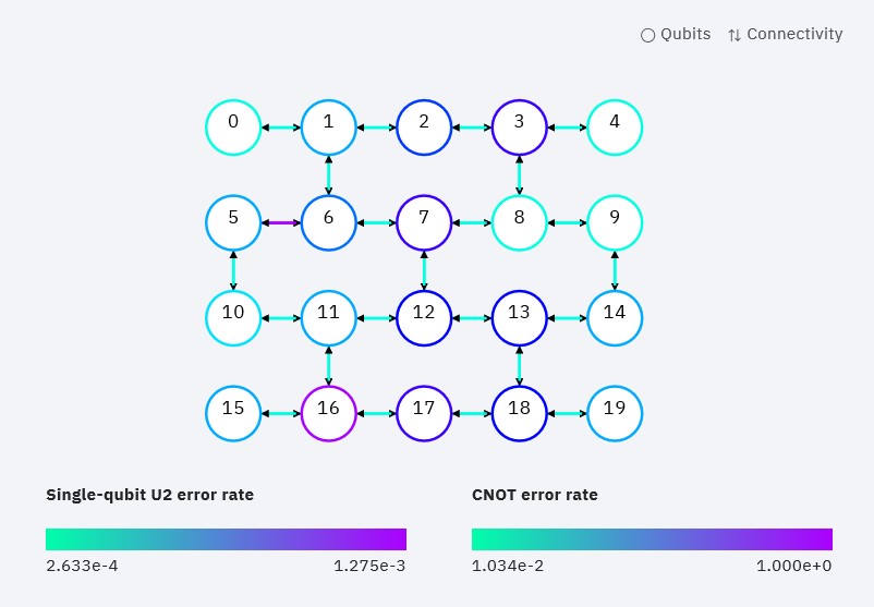
(a) IBM Q Almaden device

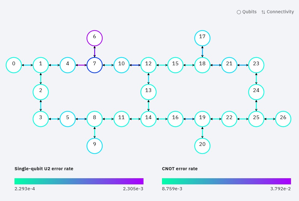
(b) IBM Q Paris device

Figure 2: Qubit connectivity with colored mappings for qubits and connections corresponding to COTD information on a heatmap range. Source: [7].

IV-B Benchmarking Circuits

We selected a number of circuits for just-in-time transpilation also used in prior work [1]. The characteristics of the selected benchmarks were based on the ability to scale single qubit gates, two-qubit gates, circuit depth and circuit width (i.e., the number of qubits). These benchmarks can be parametrized by the number of qubits, $n$, and are:

1. bv(n): the Bernstein-Vazirani algorithm that learns an $n$-bit string encoded in a function and reads out $n+1$ qubits;

2. hs(n): the n-bit/qubit hidden-shift algorithm that determines the constant by which the input of one function is increased (shifted) relative to that of another function, where $n$ qubits are measured;

3. qft(n): the n-bit/qubit quantum Fourier transform algorithm, which is used in many other quantum algorithms as a building block with $n$ qubits measured;

4. toffoli(n): the n-qubit “universal” Toffoli gate that can be specialized for a number of arithmetic operations depending on parameters, $n+1$ qubits are read out;

5. adder(n): an n-bit adder algorithm using $2\times n+2$ qubits and $n+1$ readouts.

Algorithms 1-3 include Hadamard gates and conditional rotational gates, yet still have known reference outputs. Conversely, algorithms 4-5 consist of Pauli gates, C-NOT gates or CC-NOT gates (with two conditionals), the latter of which can be transpiled into a sequence of single qubit (Hadamard and rotational) gates and six C-NOT gates, again with known expected outputs.

IV-C Qiskit Experiments

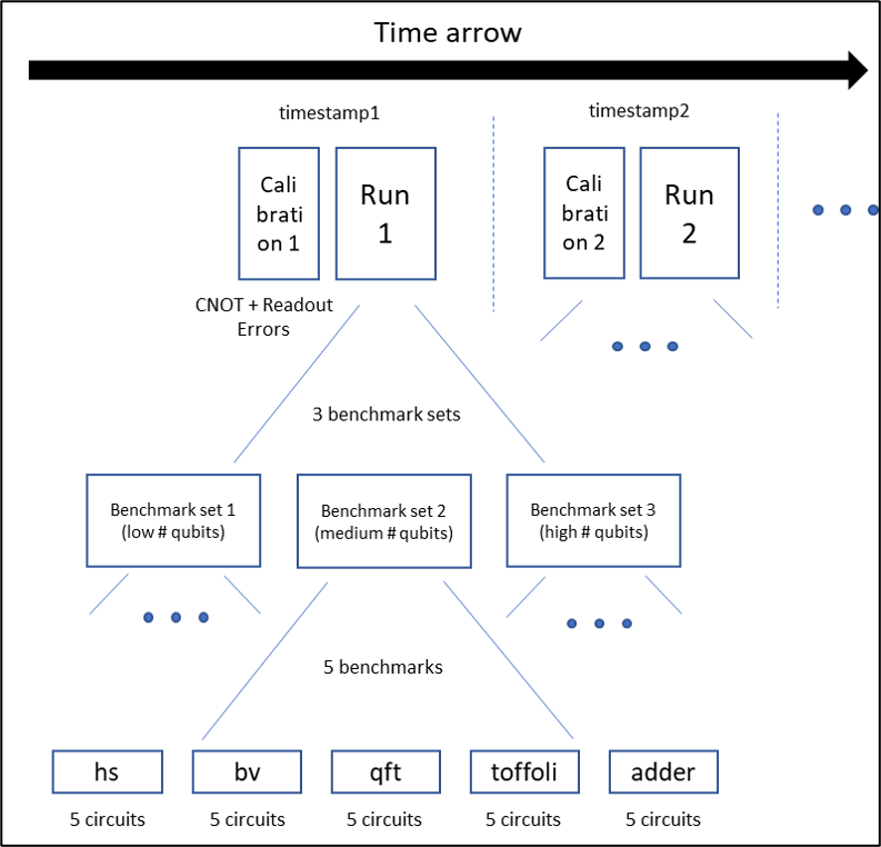
Figure 3: Calibration and benchmark circuits as arranged in our job framework

Qiskit provides an interface for sending multiple quantum circuit experiments to the device in a single job. The maximum number of these experiments depends on the type of device. As an example, the Almaden device accepts a total of 900 circuits in a single job. CNOT and readout error calibrations are performed in our experiments using the calibration circuits detailed in previous section. These are run repeatedly at a particular time of the day, as shown in Figure 3 (timestamp1, timestamp2 etc.). With the resulting error data, several benchmark circuits are transpiled. We investigate 5 circuits representing the above benchmark codes per run, where each circuit is executed for 4096 shots, i.e., repeated circuit executions with a measurement. Further, we have 3 sets of these benchmarks with increasing number of qubits as shown in the figure (low/medium/high number of qubits) in a single job. In total, a single benchmark measurement job contains 75 circuits, i.e., 25 circuits per benchmark set and 5 circuits for each individual benchmark with exactly the same circuit and mapping since they are transpiled together with the same calibration data using the qiskit.compiler.transpile function. We execute several circuits for a particular benchmark, each with 4096 shots, as we observed that for certain qubits and connections significant variations in the accuracy exist across different circuit executions within the same job. In summary, each benchmark job that gets submitted to the device is just-in-time transpiled with the latest error data obtained by our measurements — instead of the default COTD data from IBM. Depending on the experiment, these jobs are either run at different times on different days in “fairshare” queuing, or they are repeatedly run throughout the day in “dedicated” time slots to capture the variance in the accuracy of benchmark circuits. Notice that dedicated execution is a novel feature that became available only in late May 2020.

V Results

We first report results in the default user mode, followed by dedicated mode. We then perform a sensitivity analysis with respect to circuit layouts before discussing overall findings and implications.

V-A Fairshare User Mode

These experiments on IBM Q Almaden consist of a first job running all benchmarks resulting from level 3 transpilation using IBM’s error data, followed by eight instances of two jobs, one for measurement to obtain refreshed error data and a second to run all benchmarks transpiled at level 3 with the fresh error data. Percent accuracy relative to expected results (y-axis) is plotted for each benchmark run (x-axis).

Figure 4 depicts results for Hidden Shift (hs) with 4, 6, and 8 qubits, where the x-axis indicates the time (during the day) when the benchmark run started and the number of minutes prior to which error data was measured.

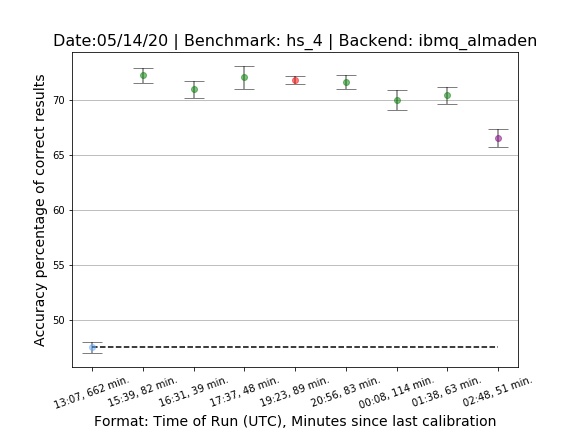
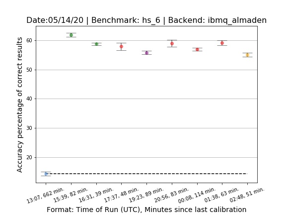
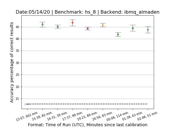
Figure 4: Accuracy of Hidden Shift for 4/6/8 qubits (upper/middle/lower graphs) at different times during the day with prior calibration in minutes.

For hs(4), the top graph in the figure, the first data point shows an accuracy of 47% (with a small standard deviation indicated by the whiskers) for IBM’s reference calibration 10 hours earlier. This is the reference run (dashed line) for our experiments. The remaining data points are showing 67-73% accuracy for our runs, spaced in 1-2 hour intervals whenever the job queue scheduled runs, with prior error data obtained 39 minutes to nearly 2 hours earlier. The different colors of data points indicate distinct layouts of virtual-to-physical qubits. Our layouts differ from IBM’s layout due to the refreshed error data, which provides the benefits in accuracy.

For hs(6) and hs(8) in middle and lower graphs of Figure 4, our results have an even higher improvement in accuracy over IBM’s reference layout, with our layouts changing from hour to hour. Overall, IBM’s accuracy is reduced from 47% to 27% to 12% for hs(4), hs(6) and hs(8), respectively. This reflects the higher number of qubits used and longer depth of a given circuit. With our just-in-time transpilation, the values are much higher: 70%, 58%, and 45% on an average for hs(4), hs(6) and hs(8), respectively.

Results for other benchmarks are similar in trend, albeit with different absolute accuracies/improvements with figures omitted due to space. Relative improvement in accuracy ranges from 8-48% for bv, 48-304% for hs, 45-69% for qft, 133-155% for toffoli, and 12-42% for adder, with maximum improvements sometimes as high as 400%, i.e., a factor of four improvement in accuracy. We also observe that toffoli, qft and adder have a higher standard deviation.

Observation 1: Just-in-time transpilation tends to improve the relative accuracy of measured results on average by 8%-304% and up to 400% in extreme cases in fairshare user mode. Best layouts change at least hourly.

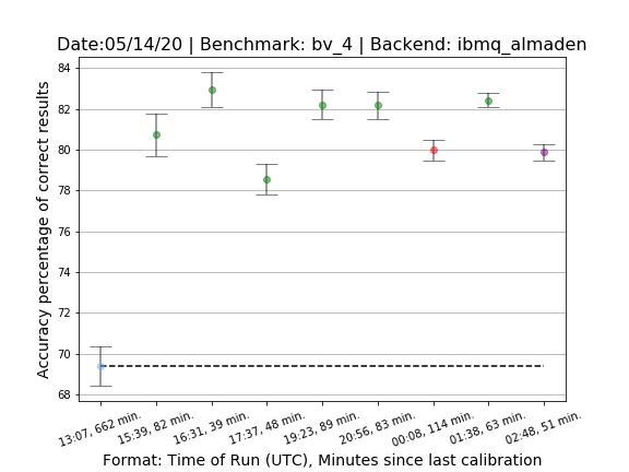
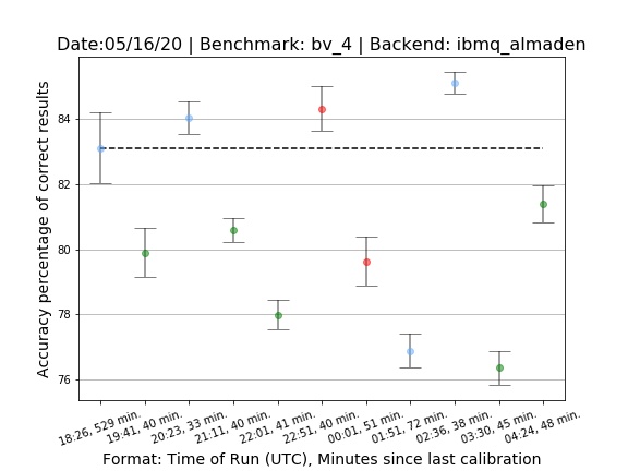
Figure 5: Accuracy of Bernstein-Vazirani with 4 Qubits on 5/14/20 (upper) and 5/16/20 (lower)

Figure 5 depicts results for Bernstein-Vazirani (bv) with 4 qubits on two different days. On the first day (upper graph), trends are similar to hidden-shift, where the accuracy of just-in-time transpiled benchmarks throughout the day is consistently higher (around 82%) than those transpiled with using IBM’s COTD (69.5%). The difference between our measurements is relatively small (+/-5%). But on a different day (lower figure), results are mixed as the benchmarks transpiled with IBM’s COTD show higher accuracy (83%) while many of our just-in-time transpilations result in lower accuracy (as little as 76%) while others are slightly better (up to 85%) than IBM’s reference. Interestingly, all the benchmarks show more significant standard deviations (wider whiskers) in the lower graph, even though IBM’s calibration was about 10 hours prior in both cases. Closer inspection reveals that the same IBM layout mapping (blue dot) also provides slightly better results (3rd and 9th data point), yet worse results at a different time (8th data point).

Observation 2: Benefits of just-in-time transpilation vary from day to day, even for the same layouts of qubits on a device.

While we observe such variation, we actually cannot provide absolute conclusions from this data as we only ran benchmarks with IBM’s COTD layout once, and only hours apart from our just-in-time experiments. This led us to conduct a set of experiments in dedicated mode close together in time, once this mode became available. This is discussed in the next subsection.

The QFT circuit (figures omitted due to space) contains a large number of two-qubit gates and thus results in lower overall accuracy and also declining accuracy as circuits are scaled up from 4 over 6 to 8 qubits. As before, IBM’s accuracy is generally lower than ours (30% vs. 18% for 4 qubits) but the total value becomes unreasonably low for 8 qubits (IBM: 0.85%, ours: 1.3%), even though our results are still better on one of the days. However, on another day, only half of our just-in-time calibrations resulted in benefits over IBM’s, still with the same low accuracy under qubit scaling. The Toffoli and adder benchmarks show trends similar to the QFT benchmark.

Observation 3: As the number of qubits is scaled up, total accuracy drops significantly to the point where few results remain correct, even with just-in-time transpilation. IBM’s results remain inferior to our just-in-time method.

V-B Dedicated Mode

In regular user mode, fairshare queuing [8] on IBM Q devices prevents a calibration job to be run back-to-back with benchmarks as just-in-time transpilation requires the error data from the calibration run, and typical queue delay is on the order of hours for IBM Q Hub devices (or even days for public devices). While we showed that qubit fidelity in terms of readout and coupling errors varies, our prior results were inconclusive with respect to the rate at which these variations take place.

A novel dedicated queuing mode allows the reservation of time slots of fixed lengths at a given time of the day. This allows us to reserve a slot long enough to run a calibration test to obtain readout and coupling errors, run benchmarks using IBM’s error data while transpiling with our newly obtained error data, and then run the just-in-time transpiled benchmarks based on our error data. These three jobs run back-to-back within 15 minutes. This experiment was repeated 8 times during a 24-hour period. Dedicated queuing was available on IBM’s Paris device with 27 qubits.

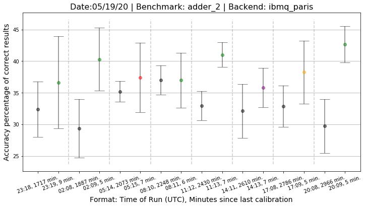
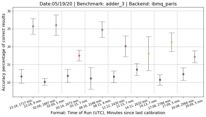
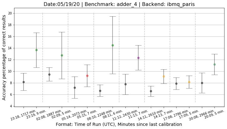
Figure 6: Accuracy of Adder for 4/6/8 qubits (upper/ middle/ lower graphs) at different times during the day with prior calibration in minutes.

Figure 6 depicts the accuracy for a 2+2, 3+3 and a 4+4 adder (upper/middle/lower graphs) in dedicated mode. Black dots indicate IBM’s layout based on their COTD errors obtained 28-49 hours earlier. Notice that the device was not recalibrated during this period, which indicates that IBM even calibrates less frequently than the 24 hours that are commonly cited. Each set of (black, colored) data points runs within the same time slot and should be related to one another in comparisons.

For the first graph, we observe that IBM runs (black) vary significantly in accuracy over time, as much as 29-37%, i.e., a given calibration with COTD error data does not provide consistent results. We further observe that when any IBM run (black) is followed by our just-in-time transpiled run (colored) minutes later, the latter always provides higher accuracy. Standard variations are sometimes higher, sometimes lower with no clear pattern. As circuit sizes are scaled up (middle/lower graphs), this trend still holds, even as absolute accuracy becomes smaller due to wider and deeper circuits. The benefits of just-in-time transpilation are more pronounced in the 3+3 adder (middle graph), without any clear cause as these three benchmarks ran back-to-back (cf. absolute times indicated on the x-axis). Just-in-time transpilation always resulted in a different circuit than IBM’s default transpilation, and the former resulted in notable savings — with the one exception of adder(4) in the 2nd to last pair of (black, yellow) dots, where our benefit is smaller. Layouts change between hourly slots. These results generalize to other benchmarks with higher (bv, hs) or lower (qft, toffoli) absolute savings. We did see occasional outliers as discussed in the next subsection. We summarize these findings as the following observation.

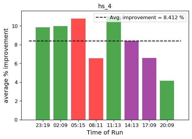
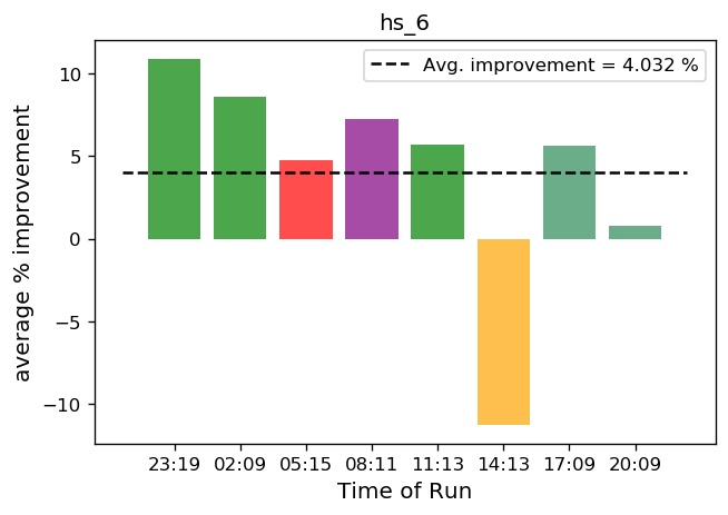
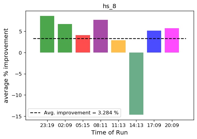
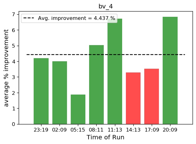
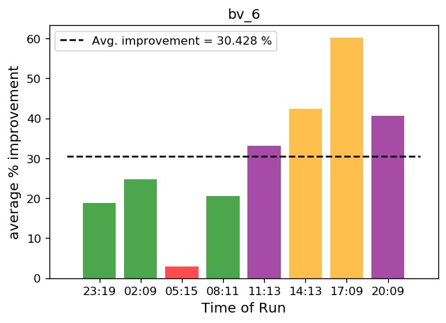
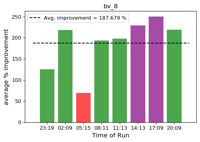
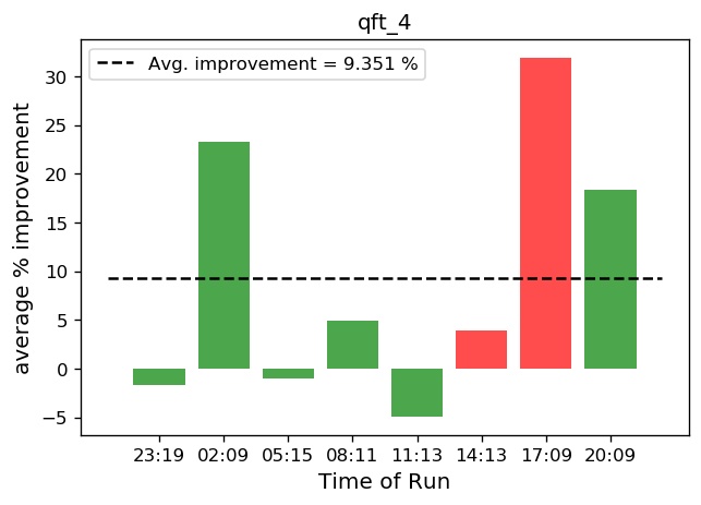
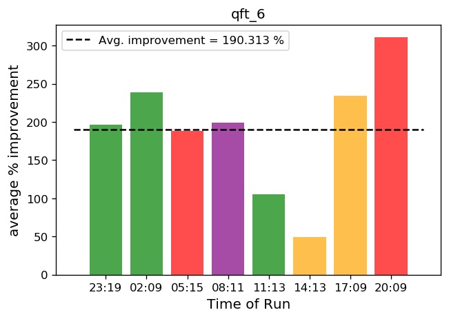
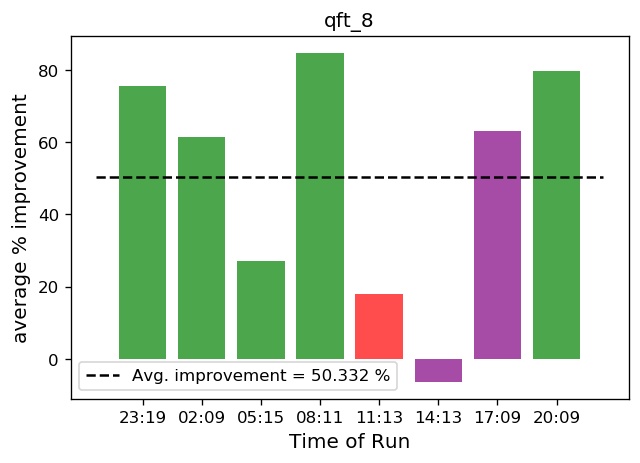
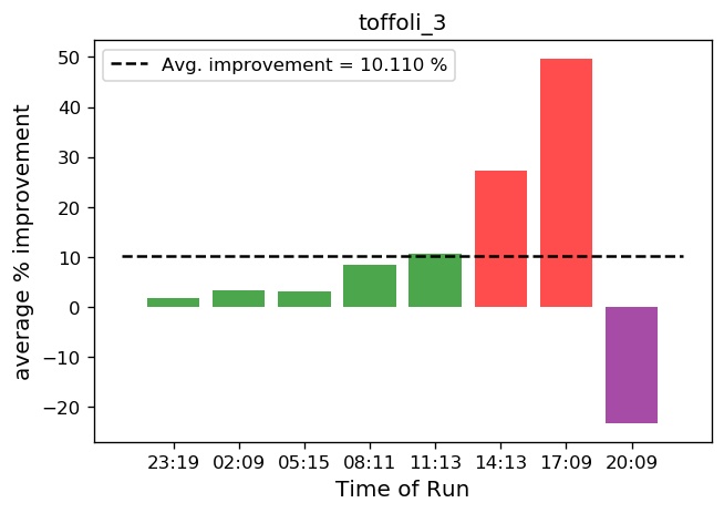
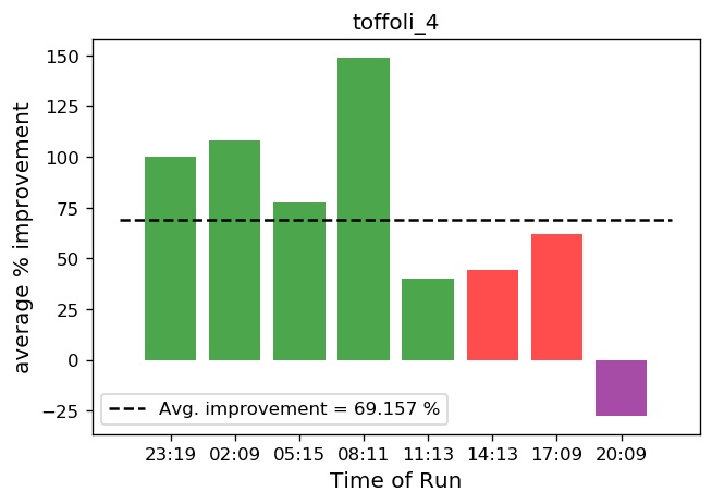
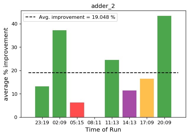
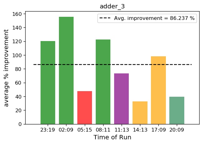
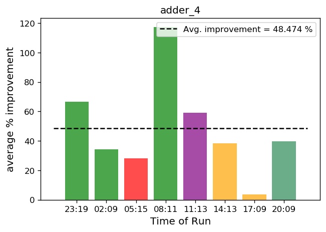
Figure 7: Percent improvement of accuracy for just-in-time transpilation in dedicated mode.

Observation 4: Just-in-time transpilation offers more significant benefits when error data is obtained immediately prior to an application circuit, irrespective of circuit width and depth.

We also conducted a sequence of experiments in a single 1-hour slot, where the IBM-transpiled benchmark was run back-to-back with four instances of (a) re-calibration (obtaining fresh error data) used by just-in-time transpilation followed by (b) executing all benchmarks. Our method was superior in all cases except for adder(4), qft(6), toffoli(3), and sometimes better/sometimes worse for qft(8).

Observation 5: Even when error data is obtained immediately prior to an application run, just-in-time transpilation cannot always guarantee to provide superior results. Variations are more pronounced long-term but also exist to a smaller extent short-term. Best layouts change even within minutes.

V-C Detailed Accuracy Improvement for Dedicated Mode

Figure 7 depicts the average percent improvement in accuracy for dedicated benchmark runs on the IBM Paris device normalized to just-in-time transpilation with IBM’s transpilation as a baseline. Each bar corresponds to a separate run in a dedicated time slot over a 24-hour period, i.e., 8 time slots in total. Different colors indicate different mappings.

Overall, most cases show a moderate to significant improvement with the occasional exception of an insignificant loss (a few instances of qft(4) and qft(8)) and few more significant losses (one instance each for hs(6), hs(8), toffoli(3), toffoli(4)). In terms of absolute accuracy, there was one data point for hs(6) where IBM’s result (59%) was better than ours (52%), and another in hs(8) with 52% vs. 44% within the same benchmark run. We do not have an explanation as neither hs(4) nor any other benchmark in the same run showed inferiority of our method. The same holds for the last run for toffoli(3) and toffoli(4). All these outliers have in common that they use a never-seen-before layout, which may indicate that the error collection method could possibly be improved on.

The overall average in improvement (over all 8 runs) is indicated by a dashed line.

Observation 6: Just-in-time transpilation tends to improve the relative accuracy of measured results on average by 3%-190% and up to 150% in extreme cases in dedicated mode. Best layouts change within minutes.

In summary, Figure 7 reinforces the last two observations in that just-in-time transpilation provides benefits in the majority of cases, but there are exceptions.

V-D Circuit Layout Analysis

Results so far have shown that differences in accuracy are correlated to just-in-time transpilation on recent error data. We investigated the benefits in a sensitivity study by considering changes in virtual-to-physical qubit mappings. To this end, the resulting virtual layouts were superimposed on the heatmap-coded interconnect of a quantum device. Figure 8 depicts pairs of IBM/our layouts for hs(8) and adder(4). The nodes are qubits and edges are couplings. A solidly colored qubit indicates that this qubit is used within the respective circuit. Heatmaps range from low errors (green) over blue to high errors (red) on a scale indicated for each graph, i.e., separately for per-qubit readouts and couplings.

Overall, we can compare the errors of the IBM model (left) with that of our error data (right) agnostic of any circuit. The error values differ for a number of qubits and couplings, most notably couplings 4-7, 6-7, 5-8, and 12-15, and also qubits 0, 4, 5, 8, 15 and 17. Others are constantly good (many qubits and couplings remain green on both sides) or constantly bad (e.g., qubit 21).

In the adder(4) example, our layout provides worse accuracy than IBM’s. First, we observe that in Figure 8(a) coupling 4-7 within the circuit has high errors (red), and qubits 5 and 8 have mediocre fidelity (blue/purple). In contrast, all couplings in Figure 8(d) are of higher fidelity (green) while only qubit 8 has lower fidelity (purple). Yet, IBM’s accuracy at 10% is better than ours at 8%. Closer inspection reveals that our lower end of the error spectrum has twice the error value of IBM’s lower end errors for both readouts and connectors. This means the color spectrum on the right side should be shifted toward higher errors. Another significant difference is in the readout qubits, which are 4,7,8,9,11 for IBM’s and 8,12,13,20,22 for our transpiled code. This accounts in part of the difference in accuracy, as will be discussed in the next subsection.

In the hs(8) example, our layout provides better accuracy than IBM’s. We observe that the selected qubits and couplings for the circuit appear nearly equally good in Figure 8(c) and Figure 8(d), with a slight bias to higher fidelity (lighter green) on the right side for qubits. As all qubits are read out, this could explain the difference, even after taking into account the differences in heatmap encoding. Notice that the hidden shift algorithm requires only pairs of two qubits to be coupled, which explains the layouts of isolated qubit pairs.

Observation 7: Differences in layouts corroborate the hypothesis that there are two classes of errors: “Persistent” errors due to low fidelity qubits and couplings that retain high errors, and “transient” errors that vary over shorter times. However, detailed analysis of layouts with respect to noise levels of qubit readouts and connectors remain only partially conclusive.

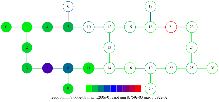
(a) IBM layout for adder(4) on Paris

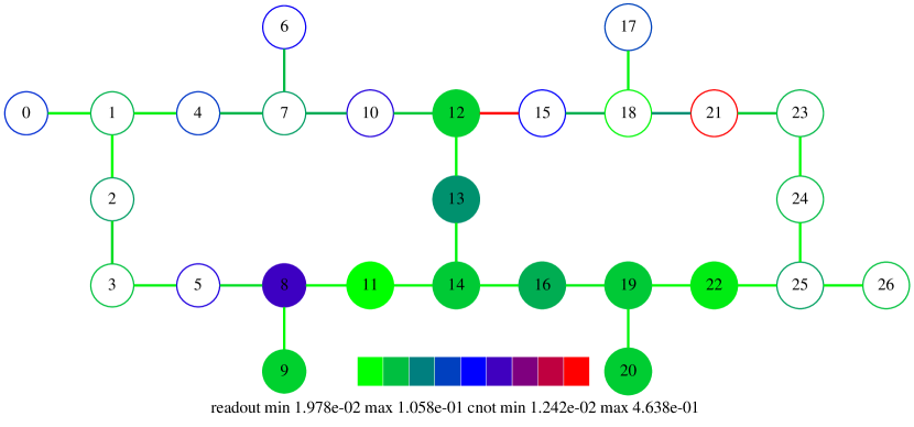
(b) Our layout for adder(4) on Paris

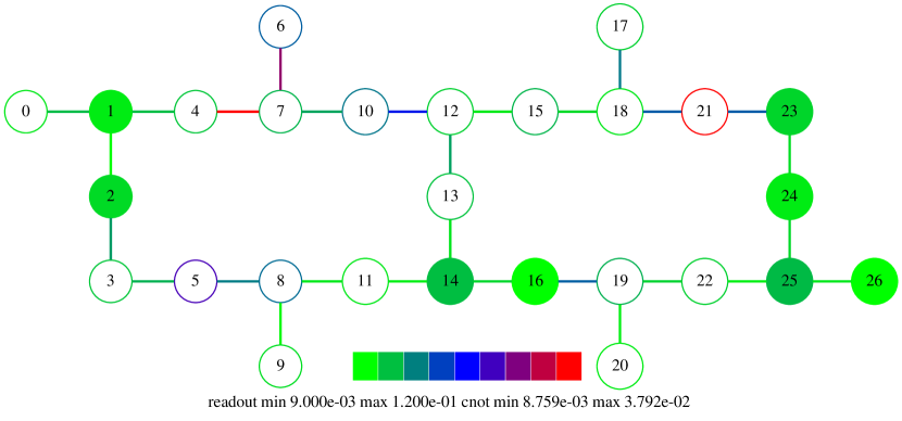
(c) IBM layout for hs(8) on Paris

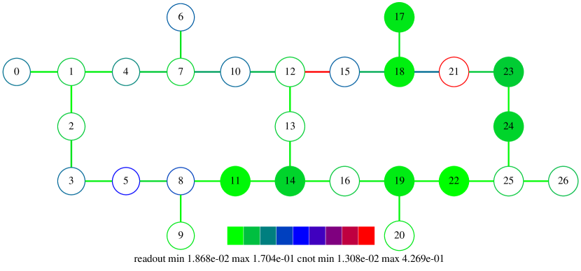
(d) Our layout for hs(8) on Paris

Figure 8: Circuit Layouts

V-E Discussion

The detailed analysis of layouts did not provide the clarity on a case-by-case basis that we had anticipated. It is possible that other factors have to be accounted for to explain differences in accuracy. In particular, it would be important to compare IBM’s codes for determining error rates with ours as we see much higher rates. This could be due to the fact that the last calibration occurred hours ago, or it could indicate that our algorithms are more suitable to find good layouts. Furthermore, cross talk error is known to be in the order of readout and coupling errors. Single qubit gate errors are said to be an order of magnitude lower, as also reported by IBM after each calibration. Another factor is the number of times a coupling is used in conditional gates (e.g., CNOT) and, to a lesser extent, the number of single qubit gates. While we saw “permanently” high qubit and coupling errors for a few device elements, most of them either remain at higher fidelity or change in the medium range over time. It may be possible to further distinguish errors within time ranges of minutes vs. hours, but we do not have sufficient data to reliably do so.

With the results shown above, we conclude that dynamic on-the-fly error calibration helps in taking into account the current state of the qubits. Transpiling the circuits just-in-time with this error information statistically produces more accurate results than those produced when the IBM’s published error information is used to transpile the same circuits.

This work has the following implications: Our approach can help in producing better results in circuits from a statistical perspective, but does not eliminate errors.

Recommendation 1: We suggest to first obtain fresh error data from a device before running sensitive circuits.

This is easily done in IBM’s dedicated mode but even provides benefits when hours lie in between obtaining error data and running the just-in-time transpiled circuit. An ensemble of circuits could then be prepared by transpiling with the dynamically measured readout error information, measured CNOT information, or both.

Recommendation 2: A circuit transpiled with the default error data should be included in experiments.

Sometimes, IBM’s layout is superior, and a diversity of mappings can provide more accurate results [4].

Recommendation 3: Devices should either be recalibrated more frequently, or their errors should be assessed more often (possibly both), with results made accessible to users.

If users always prefaced their code with a fresh error data analysis, less science could be performed on a quantum device, yet results may be of higher value. This is a subtle conundrum, and the frequency of recalibration should be revisited by quantum backend operators.

Currently, the device properties (backend.properties() object) contain the calibration information published by IBM earlier during the day. We suggest that IBM also publish more dynamic error information along with the accuracy of the circuits by periodically running these error extraction circuits. The developers could then, based on the accuracy of results, decide whether or not to exploit this dynamic error information to transpile their circuits or call their own error measurement jobs. Furthermore, noise-based transpilation (level 3 in Qiskit) should be the default. Finally, job dependencies and server-side transpilation should be introduced in fairshare user mode to allow a second job to be transpiled depending on output data of the first job that ran minutes before.

VI Related Work

Current NISQ machines require substantial tuning of control signals in order to compensate for noise in individual devices. The closest related work to ours focused on noise-aware mappings and read-out errors [1], which is using noise data to adapt qubit mappings during the transpilation process. This technique was later integrated into IBM’s Qiskit transpilation, which uses daily calibrations for qubit mappings. As our work shows, more frequent noise recalibrations provide additional benefits on today’s NISQ devices.

Other techniques focus on interpreting different qubit mappings statistically and inverting computational results to benefit from lower errors in non-excited states [4, 5], hardware-specific optimizations confined to back-end passes of the compiler across different NISQ platforms [9], or reduction in cross talk [10]. IBM uses pulses to further reduce noise [11], a technique that was generalized to larger circuits or blocks of gates with shorter pulses [12, 13].

Other qubit mapping approaches were shown to be effective for smaller-scale NISQ devices [1, 14, 2] but often required high time/memory consumption when scaling up, while others had more scalable algorithms but compromised in the fidelity of the mapping [15, 16], while yet others focused on scalability without considering noise details at the same level of detail [17], or used dynamic assertions as a means to filter by noise [18]. These techniques can orthogonally improve results on top of our recalibration.

VII Conclusion

We have contributed a methodology for on-the-fly transpilation taking fresh error data for readouts and two-qubit gates into account. Our experiments have shown the effectiveness of this technique on current NISQ devices resulting in 3-190% improvement of accuracy for dedicated execution and 8-304% for shared job queues with a maximum observed improvement of a factor of four, depending on the circuit. Improvements are best when error data was recently obtained, leading to recommendations for adjusting operations of quantum devices to obtain and publish error data more frequently.

References

- [1] P. Murali, J. M. Baker, A. J. Abhari, F. T. Chong, and M. Martonosi, “Noise-adaptive compiler mappings for noisy intermediate-scale quantum computers,” arXiv preprint arXiv:1901.11054, 2019.
- [2] S. S. Tannu and M. K. Qureshi, “Not all qubits are created equal: A case for variability-aware policies for NISQ-era quantum computers,” in Proceedings of the Twenty-Fourth International Conference on Architectural Support for Programming Languages and Operating Systems, 2019.
- [3] H. Abraham, AduOffei, I. Y. Akhalwaya, and et al., “Qiskit: An open-source framework for quantum computing,” 2019. [Online]. Available: qiskit.org
- [4] S. S. Tannu and M. K. Qureshi, “Ensemble of diverse mappings: Improving reliability of quantum computers by orchestrating dissimilar mistakes,” in International Symposium on Microarchitecture, 2019, pp. 253–265.
- [5] ——, “Mitigating measurement errors in quantum computers by exploiting state-dependent bias,” in International Symposium on Microarchitecture, 2019, pp. 279–290.
- [6] E. Magesan, J. M. Gambetta, and J. Emerson, “Scalable and robust randomized benchmarking of quantum processes,” Physical Review Letters, vol. 106, no. 18, May 2011. [Online]. Available: http://dx.doi.org/10.1103/PhysRevLett.106.180504
- [7] “IBM Quantum Experience,” https://github.com/Qiskit/qiskit-api-py, accessed: 2018-11-16.
- [8] IBM, “Fair-share queuing,” 2020. [Online]. Available: https://quantum-computing.ibm.com/docs/cloud/backends/queue
- [9] P. Murali, N. M. Linke, M. Martonosi, A. J. Abhari, N. H. Nguyen, and C. H. Alderete, “Full-stack, real-system quantum computer studies: Architectural comparisons and design insights,” in International Symposium on Computer Architecture, 2019, pp. 527–540.
- [10] P. Murali, D. C. Mckay, M. Martonosi, and A. Javadi-Abhari, “Software mitigation of crosstalk on noisy intermediate-scale quantum computers,” in Proceedings of the Twenty-Fifth International Conference on Architectural Support for Programming Languages and Operating Systems, ser. ASPLOS ’20. New York, NY, USA: Association for Computing Machinery, 2020, p. 1001–1016. [Online]. Available: https://doi.org/10.1145/3373376.3378477
- [11] L. Bishop and J. Gambetta, “Reduction and/or mitigation of crosstalk in quantum bit gates,” 2019, US Patent App. 15/721,194.
- [12] Y. Shi, N. Leung, P. Gokhale, Z. Rossi, D. I. Schuster, H. Hoffmann, and F. T. Chong, “Optimized compilation of aggregated instructions for realistic quantum computers,” in Proceedings of the Twenty-Fourth International Conference on Architectural Support for Programming Languages and Operating Systems, ser. ASPLOS ’19. New York, NY, USA: ACM, 2019, pp. 1031–1044. [Online]. Available: http://doi.acm.org/10.1145/3297858.3304018
- [13] P. Gokhale, Y. Ding, T. Propson, C. Winkler, N. Leung, Y. Shi, D. I. Schuster, H. Hoffmann, and F. T. Chong, “Partial compilation of variational algorithms for noisy intermediate-scale quantum machines,” in International Symposium on Microarchitecture, 2019.
- [14] A. Zulehner, A. Paler, and R. Wille, “An efficient methodology for mapping quantum circuits to the IBM QX architectures,” IEEE Transactions on Computer-Aided Design of Integrated Circuits and Systems, 2018.
- [15] R. Wille, O. Keszocze, M. Walter, P. Rohrs, A. Chattopadhyay, and R. Drechsler, “Look-ahead schemes for nearest neighbor optimization of 1D and 2D quantum circuits,” in 2016 21st Asia and South Pacific Design Automation Conference (ASP-DAC). IEEE, 2016, pp. 292–297.
- [16] M. Y. Siraichi, V. F. d. Santos, S. Collange, and F. M. Q. Pereira, “Qubit allocation,” in Proceedings of the 2018 International Symposium on Code Generation and Optimization. ACM, 2018, pp. 113–125.
- [17] G. Li, Y. Ding, and Y. Xie, “Tackling the qubit mapping problem for NISQ-era quantum devices,” in Proceedings of the Twenty-Fourth International Conference on Architectural Support for Programming Languages and Operating Systems, ser. ASPLOS ’19. New York, NY, USA: ACM, 2019, pp. 1001–1014. [Online]. Available: http://doi.acm.org/10.1145/3297858.3304023
- [18] J. Liu, G. T. Byrd, and H. Zhou, “Quantum circuits for dynamic runtime assertions in quantum computation,” in Proceedings of the Twenty-Fifth International Conference on Architectural Support for Programming Languages and Operating Systems, ser. ASPLOS ’20. New York, NY, USA: Association for Computing Machinery, 2020, p. 1017–1030. [Online]. Available: https://doi.org/10.1145/3373376.3378488