The Dynamics of Biological models with Optimal Harvesting

Abstract

This paper aims to introduce a concept of an equilibrium point of a dynamical system which will call it almost global asymptotically stable. A biological prey-predator model is also analyzed with a modification function growth in prey species. The conditions of the local stable and existence of all its equilibria are given. After that the model is extended to an optimal control problem to obtain an optimal harvesting strategy. The discrete time version of Pontryagin’s maximum principle is applied to solve the optimality problem. The characterization of the optimal harvesting variable and the adjoint variables are derived. Finally numerical simulations of various set of values of parameters are provided to confirm the theoretical findings.

Key Words:Global asymptotically stable,  discrete-time predator-prey system, optimal harvesting.

1 Introduction

The theory of mathematical models plays an important role for studying populations behavior. These models can be described in continuous time case or in discrete time case by a system of ordinary differential equations or a system of deference equations respectively, this description depends on the study problem . Discrete time systems are suitable for populations that reproduce at specific times each month or year or each circle, this can be seen in many insects populations, marine fish, and plants. There are variety of studies in the literature that analyzed and investigated the dynamical behavior of this kind of models, we refer to [1, 2, 3, 4],and the references therein.

The essential concept in mathematical modeling is the stability of an equilibrium point so that an equilibrium point is called globally asymptotically stable if the solution approaches to this equilibrium regardless of the initial condition, while it is called locally asymptotically stable if there exists a neighborhood of this equilibrium such that from every initial condition within this neighborhood the solution approaches to it. Some authors in the literatures([5, 6, 7, 8]) proved that the unique positive equilibrium point in their models is global asymptotically stable even one or more than one boundary equilibrium point always exits. They ignored or excluded the boundary points from the domain of the function in their biological models.In these cases they violated the definition of the global asymptotically stable. To treat this situation we introduce a definition of an equilibrium point which we call it almost global asymptotically stable, simply means an equilibrium point is global asymptotically stable in the interior of the domain.
A system of difference equations may have and show a rich and more complicated dynamical behaviors even for a simple one dimensional system. For example the logistic equation which is very known equation its equilibria can vary from stability behavior to chaotic behavior[9, 10, 11]. Many researchers investigated and analyzed different kind of two or more than two dimensional models in ecology [12, 13, 14], they derived conditions for local and global stability of solutions as well as the existence of periodic solutions [15, 16]. Some authors have discussed and assumed that the life of populations have two stages immature and adults. However stage-structured or age structured models are are considered in the literatures [17, 18, 19].
In this study we will introduce a concept of an equilibrium point of a dynamical system as well as biological model, prey predator models with modification growth function in prey species is investigated in details. The general form is given by

$$x_{t+1} =\frac{rx_{t}^{m}}{(1+ke^{bx_{t}})^{n}}-ay_{t}h(x_{t})$$ (1.1)

$$y_{t+1} =y_{t}(-c)+dh(x_{t}))$$

The continuous time version of model (1.1) can be written in the following form

$$x^{{}^{\prime}}(t) =\frac{rx(t)^{m}}{(1+ke^{bx(t)})^{n}}-ay_{t}h(x(t))$$ (1.2)

$$y^{{}^{\prime}}(t) =y(t)(-c)+dh(x(t)))$$

Where $x_{t},(x(t)),\ y_{t}(y(t))$ and $h(x_{t})$ are the prey population density, the predator population density and the predator functional response at time $t$ respectively. The parameters $r,c,a,$and $d$ are model parameters supposing only positive values.These parameters are the intrinsic growth rate of prey species, the mortality rate of predators species, the maximum per capita killing rate,and the conversion rate predator respectively.While $b,m,k$ and  $n$ are positive constants.
This paper is organized as following: In section 2 we will discuss the model (1.1) with absent the predator species when $n=m=b=1$. In section 3 the prey- predator system is analyzed and all behavior of its equilibria are investigated. In section 4 the model is extended to an optimal control problem.The discrete time version of Pontryagin’s maximum principle is applied to solve the optimality problem. In section 5 numerical simulations is provided to confirm the theoretical results. Finally conclusion is given.

2 Single species model

Definition 1.

Consider the following nonlinear discrete dynamical system $x_{t+1}=f(x_{t}),$ where  $f:D\subset R^{n}\rightarrow R^{n}$. An equilibrium point $x_{e}$, that means $f(x_{e})=x_{e}$ is said to be almost global asymptotically stable in $D$ if it is global asymptotically stable in $D-\partial D$.
For the continuous time case the definition will be as follows: Consider the following nonlinear continuous dynamical system $x^{{}^{\prime}}(t)=f(x(t)),$ where  $f:D\subset R^{n}\rightarrow R^{n}$. An equilibrium point $x_{e}$, that means $f(x_{e})=0$ is said to be almost global asymptotically stable in $D$ if it is global asymptotically stable in $D-\partial D$.

Remark 1.

1- It is clear that every global asymptotically stable is almost global asymptotically stable, and the converse is not true. For this one can see in ([7] authors proved that the positive equilibrium point $S_{3}=(x_{1}^{*},x_{2}^{*})$ there, is globally asymptotically stable only in the interior of the domain which means it is almost global asymptotically stable. However it is not global asymptotically stable because the trivial equilibrium point always exists in their model.
2- Clearly that if $x_{e}$ is almost global asymptotically stable then it is local asymptotically stable,but the converse is not true.For example :
Consider the the following system

$$x_{t+1} =s^{2}x_{t}(1-x_{t})(1-sx_{t}+sx_{t}^{2})$$

Where $s$ is constant parameter. If $s>3$ the system has two positive equilibria ,namely $x^{*}=\frac{1+s-\sqrt{(s-1)^{2}-4}}{2s}\quad\text{and}\quad y^{*}=\frac{1+s+\sqrt{(s-1)^{2}-4}}{2s}$. If $s=3.1$ then $x^{*}=0.558$ and  $y^{*}=0.7646$. The point $x^{*}=0.558$ is locally stable which is not almost global asymptotically stable point.
Now we will investigate the dynamics of single species model of (1.1) in the absent of the predator species and $n=m=b=1$. Thus the model will be as the following

$$x_{t+1} =\frac{rx_{t}}{1+ke^{x_{t}}}$$ (2.1)

The model(2.1) has two equilibria , namely, the trivial equilibrium point $x_{1}=0,$ and the unique positive point $x_{2}=ln(\frac{r-1}{k})$. The trivial equilibrium point always exists, while the positive equilibrium exists when $r>k+1$. The following lemma gives the behavior of its equilibria.

Lemma 1.

For the model (2.1) we have :

1. The trivial equilibrium point, $x_{1}=0,$ is locally stable (sink) point if and only if $r<k+1$, and it is unstable (source) point if and only if $r>k+1$,while it is non-hyperbolic point if and only if $r=k+1$.

2. The equilibrium point $x_{2}=ln(\frac{r-1}{k}),$  is locally stable (sink) point if $k\in((r-1)e^{-\frac{2r}{r-1}},(r-1))$. It is unstable (source) point if and only if $k<(r-1)e^{-\frac{2r}{r-1}}$,while it is non-hyperbolic point if and only if $k=(r-1)e^{-\frac{2r}{r-1}}$.

Proof.

It is clear that $f^{{}^{\prime}}(x_{1})=\frac{r}{k+1}$, so that the results in 1 can be easily obtained. For 2 one can see $f^{{}^{\prime}}(x_{2})=\frac{r-rx_{2}+x_{2}}{r}$ then $\mid f^{{}^{\prime}}(x_{2})\mid<1\quad\text{if and only if}\quad(r-1)e^{-\frac{2r}{r-1}}<k<r-1$ and the results can be got. ∎

Now we will consider a situations that population is exposition to harvest by a constant rate harvesting which is proportional to the respective population size therefore the model (2.1) including the harvesting will be as the following :

$$x_{t+1} =\frac{rx_{t}}{1+ke^{x_{t}}}-hx_{t}$$ (2.2)

Where $h$ is a positive constant representing the intensity of removing due to hunting or removal. It is obvious that one cannot remove more than the population density therefore $h\leq h_{max}<1,\ h_{max}$ is the maximum removing amount. The model(2.2) has also two equilibria , the trivial equilibrium point $x_{o}$,which always exists,and the unique positive equilibrium $x_{h}=ln(\frac{r-(1+h)}{k(1+h)})$ exists only when $\frac{r-(1+h)}{k(1+h)}>1$. Next lemma describes the behavior of the equilibria of model(2.2).

Lemma 2.

For the model (2.2),the equilibria, $x_{o}$, and $x_{h}$ are

1. The equilibrium point $x_{0}=0,$ is locally stable(sink) point if $r<(k+1)(1+h)$, and it is unstable(source) if $r>(k+1)(1+h)$,while it is non-hyperbolic point if $r=(k+1)(1+h)$.

2. The equilibrium point $x_{h}=ln(\frac{r-(1+h)}{k(1+h)}),$ is locally stable(sink) point if $k\in(\frac{(r-(1+h))e^{-\frac{2r}{m}}}{1+h},\frac{r-(1+h)}{1+h})$, and it is unstable(source) point if $k<\frac{(r-(1+h))e^{-\frac{2r}{m}}}{1+h}$, while it is non-hyperbolic point if $k=\frac{(r-(1+h))e^{-\frac{2r}{m}}}{1+h}$, where $m=(1+h)(r-(1+h))$.

Proof.

It is clear that $f^{{}^{\prime}}(x)=\frac{r(1+ke^{x})-rkxe^{x}}{(1+ke^{x})^{2}}-h$, then $f^{{}^{\prime}}(x_{0})=\frac{r}{(1+k)}-h$ and $f^{{}^{\prime}}(x_{h})=\frac{r+x_{h}m}{r}$, therefore all results can be obtained. ∎

3 Two Species Model,Prey-Predator Model

In this section we will study in details the dynamics of the two species model discrete time case of model (1.1) with $n=m=b=1$. Thus the system can be written as

$$x_{t+1} =\frac{rx_{t}}{(1+ke^{x_{t}})}-ay_{t}x_{t}$$ (3.1)

$$y_{t+1} =-cy_{t}+dx_{t}y_{t}$$

The all parameter $a,r,c,d$ and $k$ are defined the same as before. By solving the following algebraic equation one can get all equilibrium points of the model(3.1):

$$x =\frac{rx}{(1+ke^{x})}-ayx$$ (3.2)

$$y =-cy+dxy$$

Therefore we have the following lemma.

Lemma 3.

For all parameters values the equilibrium points of the model (3.1) are

1. The trivial equilibrium point $e_{0}=(0,0)$ always exists.

2. The boundary equilibrium point $e_{1}=(\ln(\frac{r-1}{k}),0)$ exists only when $r>1+k$.

3. The unique positive equilibrium point $e_{2}=(x^{*},y^{*})=(\frac{1+c}{d},\frac{r-(1+ke^{x^{*}})}{a(1+ke^{x^{*}})})$,which exists if $r>1+ke^{x^{*}}$.

In order to investigate the dynamic behavior of the model(3.1) one has to compute the general Jacobian matrix of the model (3.1) at point (x,y). This is given by:

$$J(x,y)=\left[\begin{array}[]{cc}J_{11}&J_{12}\\ J_{21}&J_{22}\end{array}\right]$$ (3.3)

Where $J_{11}=\frac{r+rke^{x}-rkxe^{x}}{(1+ke^{x})^{2}}-ay,\ J_{12}=-ax,\ J_{21}=dy,\ \text{and }J_{22}=dx-c$.

Next theorems give the local stability of $e_{0},\text{and}\ e_{1}$ respectively.

Theorem 1.

For the model (3.1),the equilibrium point $e_{o}$ is

1. Locally stable (sink) point if $r<(k+1)$, and $c<1$. It is unstable (source) point if $r>(k+1)$, and $c>1$,while it is non-hyperbolic point if $r=(k+1)\quad\text{or}\quad c=1$.
   

2. Saddle point if $r>(k+1)$, and $c<1$ or $r<(k+1)$, and $c>1$ .

Proof.

It is clear that the Jacobian matrix at the point $e_{0}$ is

$$J_{e_{0}}=\left[\begin{array}[]{cc}\frac{r}{1+k}&0\\ 0&-c\end{array}\right]$$

so that the eigenvalues of $J_{e_{0}}$ are $\lambda_{1}=\frac{r}{1+k}$ and $\lambda_{2}=-c$. Thus $\mid\lambda_{1}\mid<1\ (\mid\lambda_{1}\mid>1),$ if and only if $r<1+k\quad(r>1+k)$ and $\mid\lambda_{2}\mid<1\ (\mid\lambda_{2}\mid>1),$ if and only if $c<1\quad(c>1)$, as well as $\mid\lambda_{1}\mid=1\ \text{or}\quad\mid\lambda_{2}\mid=1\ \quad\text{if and only if }\ r=1+k\quad\text{or}\ c=1$. Therefore the proof is finished. ∎

Theorem 2.

For model (3.1) the equilibrium point $e1$ has the following:

1. The equilibrium point $e1$ is locally stable(sink) point if $k\in I_{1}\bigcap I_{2}$.

2. The equilibrium point $e1$ is unstable (source) if $k\in I_{3}\bigcap I_{5}$

3. The equilibrium point $e1$ is saddle point if one of the following holds:
   a)-$k\in I_{1}\bigcap I_{5}$
   b)-$k\in I_{1}\bigcap I_{4}$
   c)-$k\in I_{3}\bigcap I_{2}$
   

4. The equilibrium point $e1$ is non-hyperbolic point if $k=(r-1)e^{-\frac{2r}{r-1}},\quad\text{or}\quad k=(r-1)e^{-\frac{c+1}{d}},\quad\text{or}\quad k=(r-1)e^{-\frac{c-1}{d}}$.

where $I_{1}=((r-1)e^{-\frac{2r}{r-1}},(r-1)),\quad I_{2}=((r-1)e^{-\frac{c+1}{d}},(r-1)e^{-\frac{(c-1)}{d}}),\quad I_{3}=(0,(r-1)e^{-\frac{2r}{r-1}})\quad I_{4}=((r-1)e^{-\frac{c-1}{d}},(r-1))\ \text{and}\quad I_{5}=(0,(r-1)e^{-\frac{c+1}{d}})$

Proof.

The Jacobian matrix at the point $e_{1}$ is

$$J_{e_{1}}=\left[\begin{array}[]{cc}\frac{r-\ln(\frac{r-1}{k})}{r}&-a\ln(\frac{r-1}{k})\\ d&d\ln(\frac{r-1}{k})-c\end{array}\right]$$

then the eigenvalues of $J_{e_{1}}$ are $\lambda_{1}=\frac{r-\ln(\frac{r-1}{k})}{r},\text{and}\quad\lambda_{2}=d\ln(\frac{r-1}{k})-c$ then $\mid\lambda_{1}\mid<1\quad\text{if and only if }\quad(r-1)e^{-\frac{2r}{r-1}}<k<r-1$ and $\mid\lambda_{2}\mid<1\quad\text{if and only if }\quad(r-1)e^{-\frac{c+1}{d}}<k<(r-1)e^{-\frac{(c-1)}{d}}$. Therefore all results can be obtained directly. ∎

In order to discuss the dynamic behavior of the unique positive equilibrium, the next lemma is needed.

Lemma 4.

Let $F(\lambda)=\lambda^{2}+p\lambda+q$ Suppose that $F(1)>0,\lambda_{1},\lambda_{1}$, are roots of $F(\lambda)=0$ then
1-$\left|\lambda_{1}\right|<1$ and $\left|\lambda_{2}\right|<1$ if and only if $F(-1)>0$ and $q<1$
2-$\left|\lambda_{1}\right|>1$ and $\left|\lambda_{2}\right|<1$(or $\left|\lambda_{1}\right|<1$ and $\left|\lambda_{2}\right|>1$ ) if and only if $F(-1)<0$
3-$\left|\lambda_{1}\right|>1$ and $\left|\lambda_{2}\right|>1$if and only if $F(-1)>0$ and $q>1$
4-$\lambda_{1}=-1$ and $\left|\lambda_{2}\right|\neq 1$ if and only if $F(-1)=0$ and $p\neq 0,2$

Proof.

see[19]. ∎

Theorem 3.

For the unique positive equilibrium point $e_{2}$ of the model (3.1) we have :

1. The equilibrium point $e_{2}$ is locally asymptotically stable (sink) point if and only if $d>N,\ \text{and}\quad r\in S$.

2. The equilibrium point $e_{2}$ is unstable (source) point if and only if $d>N,\ \text{and}\quad r>max\{\frac{M_{2}}{M_{1}},\frac{N_{2}}{N_{1}},k_{1}\}$.

3. The equilibrium point $e_{2}$ is saddle point if and only if $d>N,\ \text{and}\quad k_{1}<r<\frac{M_{2}}{M_{1}}$.

4. The equilibrium point $e_{2}$ is non-hyperbolic point if these conditions are hold:
   i)-$d\neq\ \frac{2ke^{x^{*}}}{k_{1}}$
   ii)$r=\frac{M_{2}}{M_{1}}$
   iii) $r\neq\frac{2k_{1}^{2}}{kx^{*}e^{x^{*}}}\quad\text{or}\quad r\neq\frac{4k_{1}^{2}}{kx^{*}e^{x^{*}}}$.

Where $k_{1}=1+ke^{x^{*}},\quad N=\frac{2ke^{x^{*}}}{k_{1}}\quad S=(Max\{k_{1},\frac{M_{2}}{M_{1}}\},\frac{N_{2}}{N_{1}}),\quad M_{1}=dk_{1}-2x^{*}ke^{x^{*}},\ M_{2}=dx^{*}k_{1}^{2}-4k_{1}^{2},\quad N_{1}=dk_{1}-ke^{x^{*}},\quad\text{and}\quad\ N_{2}=dk_{1}^{2}$

Proof.

The Jacobian matrix at the unique positive equilibrium point is given by

$$J_{e_{2}}=\left[\begin{array}[]{cc}\frac{rk_{1}-rx^{*}ke^{x^{*}}}{k_{1}^{2}}-ay^{*}&-ax^{*}\\ dy^{*}&1\end{array}\right]$$

So that the characteristic polynomial of $J_{e_{3}}$ is

$$F(\lambda)=\lambda^{2}+p\lambda+q$$

where $p=ay^{*}+\frac{rx^{*}ke^{x^{*}}}{k_{1}^{2}}-\frac{r}{k_{1}}-1$ and  $q=\frac{r}{k_{1}}-\frac{rx^{*}ke^{x^{*}}}{k_{1}^{2}}-ay^{*}+adx^{*}y^{*}$.
It is easy to see that $F(1)=adx^{*}y^{*}$ , hence  $F(1)>0$.
Now $F(-1)>0\quad\text{if and only if}\quad 2-2ay^{*}+\frac{2r}{k_{1}}-\frac{2rx^{*}ke^{x^{*}}}{k_{1}^{2}}+adx^{*}y^{*}>0\quad\text{if and only if}\quad 4k_{1}^{2}-2rx^{*}ke^{x^{*}}+dx^{*}rk_{1}-dx^{*}k_{1}^{2}>0\quad\text{if and only if}\quad r(dx^{*}k_{1}-2kx^{*}e^{x^{*}})>dx^{*}k_{1}^{2}-4k_{1}^{2}\quad\text{if and only if}\quad r>\frac{M_{2}}{M_{1}}\quad\text{with}\quad d>N$. $\\ Q<1\quad\text{if and only if}\quad\frac{r}{k_{1}}-\frac{rx^{*}ke^{x^{*}}}{k_{1}^{2}}-ay^{*}++adx^{*}y^{*}<1\quad\text{if and only if}\quad-rkx^{*}e^{*}+dx^{*}rk_{1}-dx^{*}k^{2}_{1}<0\text{if and only if}\quad r(dx^{*}k_{1}-kx^{*}e^{x^{*}})<dx^{*}k_{1}^{2}\quad\text{if and only if}\quad r<\frac{N_{2}}{N_{1}}\quad\text{with}\quad d>N$.
According to lemma (4) the proof is finished. ∎

4 An optimal harvesting approach

In this section we will extend the model(1.1) to an optimal control problem and will discuss the optimal harvesting management of renewable resources.We assume that the population is harvested or removed with the harvesting rate $h_{t}$, which represents our control variable.
For the single species the model (2.1) including the harvesting effect becomes :

$$x_{t+1} =\frac{rx_{t}}{1+ke^{x_{t}}}-h_{t}x_{t}$$ (4.1)

The $x_{t},\ r,$ and $k$  are defined as before. In this problem the free terminal value problem is discussed and the terminal time $T$ is specified. The aim is to maximize the following objective functional

$$J(h)=\sum_{t=1}^{T-1}c_{1}h_{t}x_{t}-c_{2}h^{2}_{t}$$

where  $c_{1}h_{t}x_{t}$ represents the amount of money that one has to obtain, and $c_{2}h^{2}_{t}$ is the cost of catching and supporting the animal. $c_{1}$ and $c_{2}$ are positive constants. The control variable is subject to the constraint

$$0\leq h_{t}\leq h_{Max}$$

Now according to the discrete version of Pontryagin’s maximum principle [20], the Hamiltonian functional for this problem is given by

$$\mathcal{H}_{t} =c_{1}h_{t}x_{t}-c_{2}h^{2}_{t}+\lambda_{t+1}(\frac{rx_{t}}{1+ke^{x_{t}}}-h_{t}x_{t}),\quad t=0,1,2,....T-1$$ (4.2)

Where $\lambda_{t}=c_{1}h_{t}+\lambda_{t+1}(\frac{r+rke^{x_{t}}-rx_{t}ke^{x_{t}}}{(1+ke^{x_{t}})^{2}}-h_{t},\quad$ is the adjoint variable or shadow price[21]. Then the characterization of the optimal control solution is

$$h^{*}_{t}=\left\{\begin{array}[]{lll}0&\mbox{if }\frac{c_{1}x_{t}-\lambda_{t+1}x_{t}}{2c_{2}}\leq 0\\ \frac{c_{1}x_{t}-\lambda_{t+1}x_{t}}{2c_{2}}&\mbox{if }0<\frac{c_{1}x_{t}-\lambda_{t+1}x_{t}}{2c_{2}}<h_{Max}\\ h_{Max}&\mbox{if }h_{Max}<\frac{c_{1}x_{t}-\lambda_{t+1}x_{t}}{2c_{2}}\end{array}\right.$$

In order to extend the two species model to an optimal control problem, the model (3.1)with control harvesting variable will become as the following:

$$x_{t+1} =\frac{rx_{t}}{(1+ke^{x_{t}})}-ay_{t}x_{t}-h_{t}x_{t}$$ (4.3)

$$y_{t+1} =-cy_{t}+dx_{t}y_{t}$$

Our aim in this problem is to get an optimal harvesting amount for that we will maximize the following cost functional

$$J(h_{t})=\sum_{t=1}^{T-1}c_{1}h_{t}x_{t}-c_{2}h^{2}_{t}$$

subject to the state equations (4.3) with control constraint

$$0\leq h_{t}\leq h_{Max}<1$$

All terms and parameters are as before.So that the Hamiltonian functional will be as the following:

$$\mathcal{H}_{t} =\sum_{t=1}^{T-1}c_{1}h_{t}x_{t}-c_{2}h^{2}_{t}+\lambda_{1,t+1}(\frac{rx_{t}}{1+ke^{x_{t}}}-h_{t}x_{t})$$ (4.4)

$$+\lambda_{2,t+1}(-cy_{t}+dx_{t}y_{t})$$

Where $\lambda_{1}$ and $\lambda_{2}$ are the adjoint functions that satisfy :

$$\lambda_{1,t} =c_{1}h_{t}+\lambda_{1,t+1}(\frac{r+rke^{x_{t}}-rx_{t}ke^{x_{t}}}{(1+ke^{x_{t}})^{2}}-h_{t})+\lambda_{2,t+1}dy_{t}$$ (4.5)

$$\lambda_{2,t} =\lambda_{1,t+1}(-a_{1}x_{t})+\lambda_{2,t+1}(-c+dx_{t})$$

$$\lambda_{1,T} =\lambda_{2,T}=0.$$

Furthermore the characterization of the optimal harvesting solution $h^{*}$ satisfies:

$$h^{*}_{t}=\left\{\begin{array}[]{lll}0&\mbox{if }\frac{x_{t}(c_{1}-\lambda_{1,t+1})}{2c_{2}}\leq 0\\ \frac{x_{t}(c_{1}-\lambda_{1,t+1})}{2c_{2}}&\mbox{if }0<\frac{x_{t}(c_{1}-\lambda_{1,t+1})}{2c_{2}}<h_{Max}\\ h_{Max}&\mbox{if }h_{Max}<\frac{x_{t}(c_{1}-\lambda_{1,t+1})}{2c_{2}}\end{array}\right.$$

An iterative method in [20] is used to get the optimal control with corresponding optimal state solutions of the above optimal control problems at time $t$ by maximizing the Hamiltonian functional at that $t$ numerically.

5 Numerical Simulations

In this section we will illustrate the theoretical findings numerically for various set of parameters. For the local stability of the equilibrium point $e_{0}$ of the model(3.1), we choose this set of values $a=.1;r=0.9;k=0.01;d=1.2;c=0.01\quad\text{and}\quad(x_{0},y_{0})=(0.3,0.01)$ so that by (1) in theorem(1) the point is sink. For the equilibrium point $e_{1}$ this set of values $r=1.9;a=0.1;;c=0.2,d=2,k=0.6\quad\text{and}\quad(x_{0},y_{0})=(0.9,0.4)$ are used. Then according to the condition (1) in theorem (2) the point is sink. Figures 1-2 show the locally stability of $e_{0}$ ,and $e_{1}$ respectively. For the unique positive equilibrium point $e_{2}$ the set of values $r=5;a=.1;k=2;c=.61;d=3;\quad\text{and}\quad(x0,y0)=(0.53,1.9)$ are chosen. According to (1) in theorem (3). The local stability of $e_{2}$ is shown in Figure 3. Other sets of values can be chosen to show the local stability of $e_{0},\ e_{1}\quad\text{and}\quad e_{2}$.
For the optimal control problem an iterative numerical method in [20] is used to determine the optimal solutions with corresponding state solutions. For the control problem of single species we choose this set of values of parameters $r=1.999;k=.8;c1=0.1;c2=0.01,x_{0}=0.1\quad\text{and}\quad T=80$ so that the total optimal objective functional $Jopt$ is found equal to $0.0412$. In Figure 4 the prey population density with control , without control and with constant harvesting is plotted. Figure 5 shows the control variable as a function of time.
For the optimal control problem of two species model we choose this set of values of parameters $a=0.1;k=2.1;c=0.5;d=2.9;r=5.2;c1=0.025;c2=0.08,(x_{0},y_{0})=(0.5,0.8)\quad\text{and}\quad T=80$. So that the total optimal objective functional $Jopt$ is found equal to $0.04121$. Figures 6-7 shows the prey population and the predator population with control ,without control and with constant control respectively, and Figure 8 shows the control variable as a function of time.
Finally Table 1 contains the total optimal objective functional and other different total harvesting amount strategies of both control problems by using the same values of the parameters in each problem.

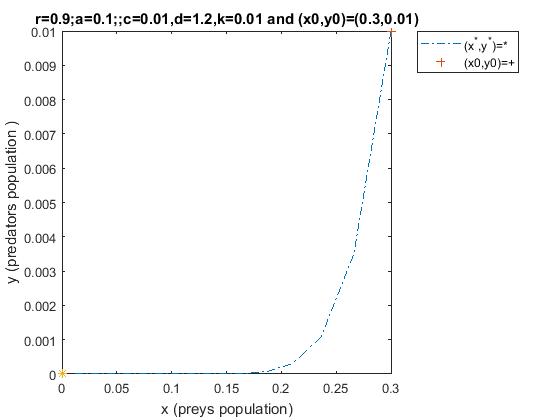
Figure 1: This figure shows the local stability of the equilibrium point $e_{0}$ of the model (3.1).

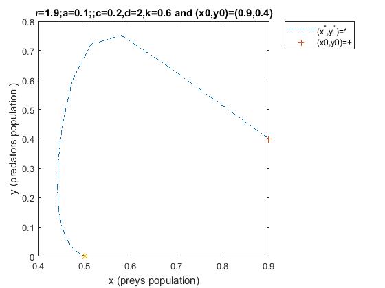
Figure 2: This figure shows the local stability of the equilibrium point $e_{1}$ of the model (3.1)

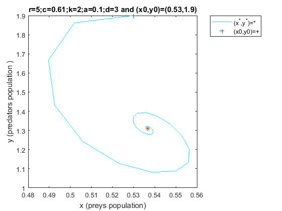
Figure 3: This figure shows the local stability of the unique equilibrium point $e_{2}$ of the model (3.1)

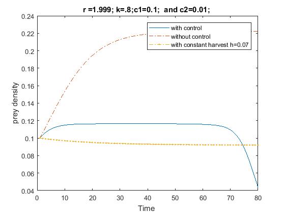
Figure 4: This figure shows the affect of different harvesting variables on the prey density in model (4.1). All values of parameters are the same in all cases.

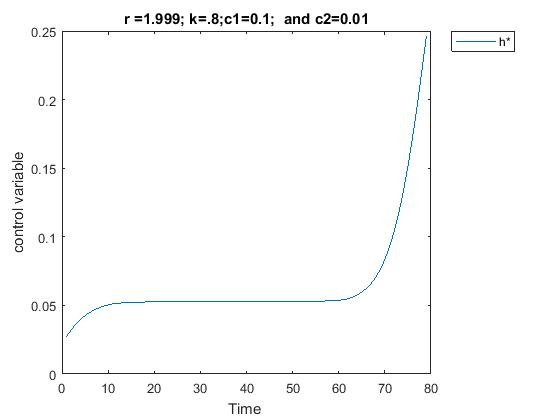
Figure 5: The optimal control variable of single species problem is shown function of time.

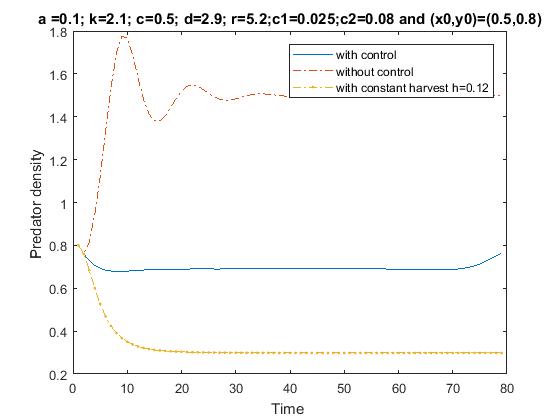
Figure 6: This figure shows the affect of harvesting variable on the predator density in model (4.3). All values of parameters are the same

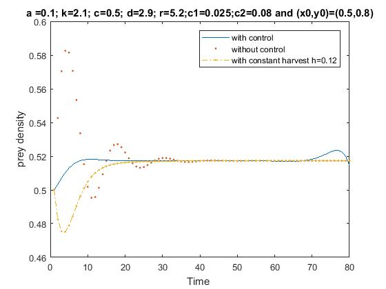
Figure 7: This figure shows the affect of different harvesting variables on the prey density in model (4.3). All values of parameters are the same in all cases.

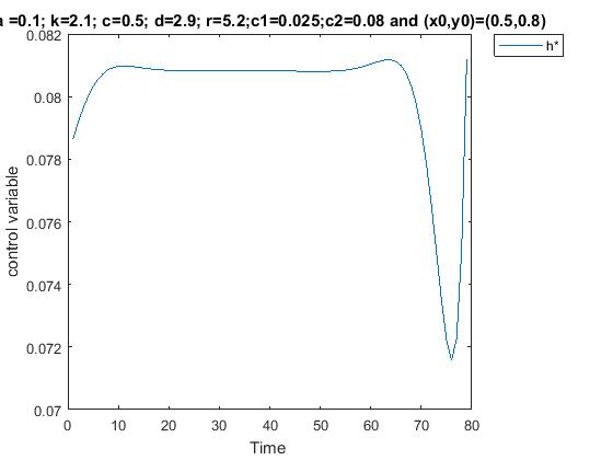
Figure 8: This shows the optimal control solution of two species problem as function of time

single species model		Two species model
The harvesting variable	The objective functional (J)	The harvesting variable	The objective functional(J)
$h_{t}=h*$	$Jopt=0.0491$	$h_{t}=h*$	$Jopt=0.04121$
$h_{t}=0.065$	$J=0.0449$	$h_{t}=0.12$	$J=0.0306$
$h_{t}=0.06$	$J=0.04524$	$h_{t}=0.1$	$J=0.0386$
$h_{t}=0.058$	$J=0.04522$	$h_{t}=0.09$	$J=0.04052$
$h_{t}=0.055$	$J=0.0450$	$h_{t}=0.08$	$J=0.04118$
$h_{t}=0.05$	$J=0.0442$	$h_{t}=0.07$	$J=0.04054$

Table 1: This table shows the results of the optimal harvesting amount with different constant harvesting.

6 Conclusion

In this paper the definition of almost global asymptotically stable of an equilibrium point is introduced with examples. We have also investigate biological models in discrete time case for one species with a modification growth function and for two species, prey-predator, model.We have studied the dynamics behavior of the equilibrium points for each model. after that we have extended these model to an optimal control problems. We have used the Pontaygin’s principle maximum to get the optimal solutions numerically. Finally one can investigate the dynamics behavior of the continuous time case as well as the other values of $n,m,$ and $b$ in future work.

References

- [1] BS Goh. Global stability in two species interactions. Journal of Mathematical Biology, 3(3-4):313–318, 1976.
- [2] Alan Hastings. Population biology: concepts and models. Springer Science & Business Media, 2013.
- [3] TK Kar and UK Pahari. Modelling and analysis of a prey–predator system with stage-structure and harvesting. Nonlinear Analysis: Real World Applications, 8(2):601–609, 2007.
- [4] Ghosoon M Hamoudi and Sadiq Al-Nassir. Dynamics and an optimal policy for a discrete time system with ricker growth. Iraqi Journal of Science, 60(1):135–142, 2019.
- [5] MA Aziz-Alaoui. Study of a leslie–gower-type tritrophic population model. Chaos, Solitons & Fractals, 14(8):1275–1293, 2002.
- [6] Jim M Cushing. An evolutionary beverton-holt model. In Theory and Applications of Difference Equations and Discrete Dynamical Systems, pages 127–141. Springer, 2014.
- [7] Tapasi Das, RN Mukherjee, and KS Chaudhuri. Bioeconomic harvesting of a prey–predator fishery. Journal of biological dynamics, 3(5):447–462, 2009.
- [8] Lingshu Wang, Rui Xu, and Guanghui Feng. Global dynamics of a delayed predator–prey model with stage structure and holling type ii functional response. Journal of Applied Mathematics and Computing, 47(1-2):73–89, 2015.
- [9] Robert M May. Simple mathematical models with very complicated dynamics. Nature, 261(5560):459–467, 1976.
- [10] Gian Italo Bischi, Laura Gardini, and Michael Kopel. Analysis of global bifurcations in a market share attraction model. Journal of Economic Dynamics and Control, 24(5-7):855–879, 2000.
- [11] Tönu Puu. Attractors, bifurcations, & chaos: Nonlinear phenomena in economics. Springer Science & Business Media, 2013.
- [12] Kondalsamy Gopalsamy. Stability and oscillations in delay differential equations of population dynamics, volume 74. Springer Science & Business Media, 2013.
- [13] John Guckenheimer and Philip Holmes. Nonlinear oscillations, dynamical systems, and bifurcations of vector fields, volume 42. Springer Science & Business Media, 2013.
- [14] Xiaoli Liu and Dongmei Xiao. Complex dynamic behaviors of a discrete-time predator–prey system. Chaos, Solitons & Fractals, 32(1):80–94, 2007.
- [15] Hai-Feng Huo and Wan-Tong Li. Existence and global stability of periodic solutions of a discrete predator–prey system with delays. Applied Mathematics and Computation, 153(2):337–351, 2004.
- [16] Xiuxiang Liu. A note on the existence of periodic solutions in discrete predator–prey models. Applied Mathematical Modelling, 34(9):2477–2483, 2010.
- [17] Arild Wikan. On nonlinear age-and stage-structured population models. Journal of Mathematics and Statistics, 8(2):311–322, 2012.
- [18] Arild Wikan and Einar Mjølhus. Periodicity of 4 in age-structured population models with density dependence. Journal of Theoretical Biology, 173(2):109–119, 1995.
- [19] Yan Ni Xiao and Lan Sun Chen. Global stability of a predator-prey system with stage structure for the predator. Acta Mathematica Sinica, 20(1):63–70, 2004.
- [20] Suzanne Lenhart and John T Workman. Optimal control applied to biological models. CRC press, 2007.
- [21] Colin Whitcomb Clark. Bioeconomic modelling and fisheries management. 1985.