A Bayesian Approach for Predicting Food and Beverage Sales in Staff Canteens and Restaurants

Abstract

Accurate demand forecasting is one of the key aspects for successfully managing restaurants and staff canteens. In particular, properly predicting future sales of menu items allows a precise ordering of food stock. From an environmental point of view, this ensures maintaining a low level of pre-consumer food waste, while from the managerial point of view, this is critical to guarantee the profitability of the restaurant. Hence, we are interested in predicting future values of the daily sold quantities of given menu items. The corresponding time series show multiple strong seasonalities, trend changes, data gaps, and outliers. We propose a forecasting approach that is solely based on the data retrieved from Point of Sales systems and allows for a straightforward human interpretation. Therefore, we propose two generalized additive models for predicting the future sales. In an extensive evaluation, we consider two data sets collected at a casual restaurant and a large staff canteen consisting of multiple time series, that cover a period of 20 months, respectively. We show that the proposed models fit the features of the considered restaurant data. Moreover, we compare the predictive performance of our method against the performance of other well-established forecasting approaches.

Keywords: Sales Prediction; Time Series; Generalized Additive Models; Bayesian Methods; Shrinkage Priors

1 Introduction

The total turnover in the US restaurants sector is projected to reach $\$863\text{bn}$ in 2019, contributing to $4\,\%$ of the gross domestic product [2]. Currently, the restaurant industry employs $15.3$ million people at one million locations across the United States. At the same time, the industry accounts for $11.4$ million tons of food waste that constitutes an estimated value of $\$25\text{bn}$ going to waste [3] every year.

Food waste is a critical socioeconomic problem considering that $11.8\,\%$ of the households in the U.S. suffered from food insecurity in 2018 [9]. Furthermore, production, transportation, and disposal of unused food significantly impact the environment [1, 18]. On the other hand, food costs represent $28\,\%$ to $35\,\%$ of sales in restaurants. Hence, reducing food waste can be critical to boost profitability and to reduce the environmental impact of operating a restaurant. Furthermore, also food service contractors face similar challenges when providing meals at staff canteens, hospitals, etc.

Accurate demand forecasting is one of the key aspects for successfully managing restaurants and, from an environmental point of view, maintaining a low level of pre-consumer food waste. In this work, we are interested in predicting future values of the daily sold quantities of a given menu item. Hence, we deal with time series that show multiple strong seasonalities, trend changes, and outliers. Traditionally, judgmental forecasting techniques, based on the managers experience, are applied to estimate future demand at restaurants. However, producing high quality forecasts is a time consuming and challenging task, especially for inexperienced managers. Hence, we aim for a data-driven approach that supports restaurant managers in their decision making.

Nowadays, most restaurants and canteens use (electronic) Point of Sales (POS) systems to keep track of all their sales. Clearly, the resulting data inventories are valuable sources for various data science applications such as forecasting future sales numbers of menu items. In general, many industries rely on POS data to predict future demand. However, especially in the retailing sector, it is hard to make beneficial use of these estimates due to complicated supply chains and long lead times. In contrast to that, the restaurant industry is characterized by short lead times when ordering food stock and the absence of a complex supply chain.

Hence, we propose a forecasting approach that requires only POS data, i.e., weather information and special promotions are not considered. Moreover, in order to ensure acceptance of the approach among restaurant managers, the models ability for a straightforward human interpretation is critical.

The remainder of this paper is organized as follows. First, in Section 2, we provide a concise problem description. In Section 3, we briefly discuss related literature. Then, in Section 4, we propose our forecasting approach. In Section 5, we evaluate the prediction quality of our approach using real-world data of sales in a restaurant and a canteen. Finally, Section 6 concludes the paper and outlines future research directions.

2 Problem Description

This work is concerned with predicting the daily sold quantities of given menu items. This information, together with the recipes of the items, is essential to effectively manage the ordering of food stock. In our use-case, an (electronic) Point of Sales (POS) system is the exclusive data source. Typically, such systems create a new line item for each sold menu item together with a time stamp. This way, large data inventories, consisting of thousands of line items, are created. Each restaurant, let it be a small burger joint or a large company canteen, usually has many different products on its menu. While some products are offered all year long, others are only seasonally available. Moreover, the demand for certain products differs over the year.

Each menu item is usually identified through an unique ID. From the stored records, we can query the accumulated number of sales of the different menu items for each day. Hence, gathering the data required for our forecasting approach causes little to no additional administrative burden. In some cases, it is reasonable to do forecasting for product groups rather than for individual menu items. For example, a canteen may have a daily vegetarian option. Each day a different dish, identified by its own ID, is served.

2.1 Assumptions

For now, we assume that the sales of individual menu items are independent of each other. While this assumption is unlikely to be true for all types of restaurants, e.g., some sides go along better with certain main dishes than others, it is a reasonable simplifying assumption.

By design, a POS system only documents sales. The absence of recorded sales of a certain menu item on a given day may be due to several reasons:

1. The restaurant was closed. In this case, there is no recorded sale of any item at all.

2. The item was not on the menu that day by choice or due to lack of stock.

3. Nobody wanted to order the product.

Obviously, it makes a difference if a product was not sold due to the fact that nobody wanted to order it (iii), or due to the reason that the product was not offered (i, ii). To distinguish between these to cases we treat an absence of sales caused by (iii) as zero sales and the absence of sales caused by (i) or (ii) as missing values. Setting the number of sales independently of (i), (ii), or (iii) always equal to zero can lead to inferior model fits, especially if the periods where the restaurant is closed, or does not offer special products, are aperiodic, or do not show a common pattern. For sure, this could be prevented by adding some information regarding why there are no sales to the model. However, this would require to manage and store additional data other than the POS data, which we do not want to presuppose in this work.

We assume that the restaurant was opened for business on a given day if there is at least one recorded sale of any menu item. Usually, data available from a POS system contains no records about when a product was added to and when it was removed from the menu. Therefore, we assume that an item has been removed from the menu if there is no recorded sale for $60$ or more days.

3 Related Work

In this section, we give a brief overview of related literature. We focus on forecasting approaches used in the restaurant industry as well as on the use of POS data.

A general view of forecasting methods for restaurant sales and customer demand is given in the recent review paper by Lasek et al. [29]. Ryu and Sanchez [37] compare several methods (moving average, multiple regression, exponential smoothing) in order to estimate the daily dinner counts at a university dinning center. In their case, a study shows that multiple regression gives the most accurate predictions. Also, Reynolds et al. [35] use multiple regression to predict the annual sales volume of the restaurant industry (and of certain subsegments). Forst [13] applies ARIMA and exponential smoothing models to forecast the weekly sales (in USD) at a small campus restaurant. Hu et al. [21] use ARIMA methods to predict the customer count at casino buffets. Cranage and Andrew [11] use exponential smoothing to predict the monthly sales (in USD) at a restaurant. Bujisic et al. [5] analyze the effects of weather factors onto restaurant sales. The paper also contains a review of forecasting approaches for restaurant sales (with and without weather factors). However, the authors point out that most work from the literature is concerned with aggregated forecasts, i.e., only predictions for product categories or weekly sales numbers are given, rather than forecasting sales of individual menu items per day.

Moreover, Tanizaki et al. [41] propose to use machine learning techniques in order to forecast the daily number of customers at restaurants. Their predictions are based on POS data that is enriched with external data, e.g., weather information and event data. Similarly, Kaneko and Yada [26] present a deep learning approach to construct a prediction model for the sales at supermarkets using POS data.

So far, this short review shows that existing work in the literature is mostly concerned with predicting aggregated numbers rather than the sale of individual items. Moreover, it reveals that using POS data is common practice in many industries. However, our review exposes a gap in the existing literature as, to the best of our knowledge, there exists no work concerned with predicting sales of individual menu items at restaurants (based on POS data).

Hence, we extend our review onto prediction approaches dealing with data showing similar features than ours. The problem considered in this work is clearly a time series prediction problem. Its most dominant characteristics are: multiple strong seasonalities, trend changes, data gaps, and outliers. Thus, the application of classical time series models such as ARIMA models or exponential smoothing [20] is of limited use. These models can only account for one seasonality and, moreover, require missing data points to be interpolated. In principle, multiple seasonality patterns can be dealt with in exponential smoothing, see e.g., Gould et al. [16]. However, most available ARIMA or exponential smoothing implementations, e.g., [23, 22], do not include such features.

Therefore, Taylor and Letham [42] present a decomposable time series model that is similar to a generalized additive model [17]. It consists of three main components: trend, seasonality, and holidays. The model is designed in such a way that it allows for a straightforward human interpretation for each parameter allowing an analyst to adjust the model if necessary. The approach is concerned with time series having features such as multiple strong seasonalities, trend changes, outliers, and holiday effects. As a motivating example they use a time series describing the number of events that are created on Facebook every day. However, this number is quite large in comparison to the daily sales in restaurants and canteens. Thus, for Facebook’s example it is valid to assign a normal distribution to the target variable. However, this might be inferior in our use case, since small target values are quite common. Note that the normal distribution $\mathcal{N}(\lambda,\lambda)$ has a shape similar to the Poisson distribution $Poisson(\lambda)$ for large $\lambda$. In contrast to the normal distribution, the Poisson distribution is a classical distribution for count data.

4 Methodology

In this section, we propose two Bayesian generalized additive models (GAMs) for demand prediction. The first one assumes a normally distributed target (also called response) $y$, the second one assumes that the response $y$ follows a negative binomial distribution. Both models include a trend function $g(t)$ and a seasonality function $s(t)$. Sparsity inducing priors [33, 7] are assigned to the parameters of $g(t)$ and $s(t)$. This allows for a good model regularization, selection of significant trend changes or influential seasonal effects, and, finally, enhanced model interpretability.

Considering that restaurants and canteens commonly offer many different menu items and that new data is recorded on a daily basis, multiple models have to be trained on a frequent basis. For this reason, the training process should require only little computation time. Additionally, the inference should take place automatically without the drawback that a human analyst has to investigate the convergence of the procedure. Therefore, we consider the application of full Bayesian inference as inappropriate and focus on the comparatively easy to obtain mode of the posterior, the so-called maximum a posteriori (MAP) estimate, instead.

4.1 Generalized Additive Models

A generalized additive model writes as

$$g(\mathbb{E}(y))=\beta_{0}+\beta_{1}x_{1}+\ldots+\beta_{k}x_{k}+f_{1}(z_{1})+\ldots+f_{q}(z_{q}),$$

where $y$ denotes the target variable corresponding to some exponential family distribution, $x_{1},\ldots,\allowbreak x_{k},z_{1},\ldots,x_{k}\in\mathbb{R}$ denote the predictors (also called covariates), $g$ denotes a link function (bijective and twice differentiable), and $f_{1},\ldots,f_{q}$ denote some smooth functions. Typically, the functions $f_{i}$ are defined as weighted sums of basis functions, i.e., $f_{i}=\sum_{k=1}^{K_{i}}\gamma_{ik}B_{ik}(z_{i}).$ Sparsity inducing priors can be used to perform variable selection within the set $\{x_{1},\ldots,x_{k}\}$ and, further, appropriate priors can be used to control the smoothness of the functions $f_{1},\ldots,f_{q}$.

4.2 Trend Function

To model the trend of a time series, i.e., a series of data points ordered in time, we use a polynomial spline $g$ of degree $l$, see Fahrmeir et al. [12].

A mapping $g:[a,b]\rightarrow\mathbb{R}$ is called polynomial spline of degree (order) $l\geq 0$ with knot points at $k_{1}<\ldots<k_{m}$, ($a<k_{1},k_{m}<b$), if

1. $g$ is a polynomial of degree $l$ on each of the intervals $[a,k_{1})$, $[k_{1},k_{2})$,…, $[k_{m},b)$, and

2. $g$ is $l-1$ times continuously differentiable provided that $l>0$.

Let $S_{l}^{\mathbf{k}}$ denote the set of all $l$-th order splines with knots given by $k_{1}<\ldots<k_{m}$. Equipped with the operations of adding two functions and taking real multiples $S_{l}^{\mathbf{k}}$ is a real vector space. One can show that each element of $S_{l}^{\mathbf{k}}$ can be uniquely written as linear combination of the $d=l+m+1$ functions

$$B_{1}(t) =1,\leavevmode\nobreak\ B_{2}(t)=t,\ldots,\leavevmode\nobreak\ B_{l+1}(t)=t^{l},$$

$$B_{(l+2)}(t) =(t-k_{1})_{+}^{l},\ldots,\leavevmode\nobreak\ B_{(l+m+1)}(t)=(t-k_{m})_{+}^{l},$$

where

$$(t-k_{j})_{+}^{l} =\begin{cases}(t-k_{j})^{l},&t\geq k_{j},\\ 0,&\text{else}.\end{cases}$$

For this reason, the functions $B_{1},\ldots,B_{d}$ build a basis $B$ of the spline space $S_{l}^{\mathbf{k}}$. $B$ is called the truncated power series basis (TP-basis). The TP-basis allows for a simple interpretation of the trend model

$$g(t) =\sum\limits_{j=1}^{d}\gamma_{j}B_{j}(t)$$ (1)

$$=\gamma_{1}+\gamma_{2}t+\ldots+\gamma_{l+1}t^{l}+\gamma_{l+2}(t-k_{1})_{+}^{l}+\ldots+\gamma_{l+m+1}(t-k_{m})_{+}^{l}.$$

The trend model $g$ consists of a global polynomial of degree $l$ which changes at each knot $k_{j}$. The amount of change at a given knot point $k_{j}$ is determined by the absolute value of the corresponding coefficient $\gamma_{l+j+1}$. Thus, the knots of the polynomial spline are interpreted as (possible) change points in the trend.

As a consequence, the assignment of a sparsity inducing prior to the trend coefficients $\gamma_{1},\gamma_{2},\ldots,\allowbreak\gamma_{d}$ would allow for an identification of truly significant trend changes. This increases the interpretability of the model and also regularizes the trend function.

According to domain experts, for most menu items the trend (regarding the number of sales) is quite constant over long periods, while significant changes appear only occasionally. Hence, we decide to specify a knot point every $k$-th day between the first and the last date with observations. Assuming that the trend may change on a weekly basis, a possible value for $k$ could be $k=7$. However, for restaurants that observe only slight changes once in a while also larger values for $k$ are useful in order to reduce the size of the resulting model. Consequently, we choose $k=30$ in our experimental evaluation, see Section 5.4.3.

4.2.1 Prior for the Trend

In this section, we propose two different priors for the trend model. The first one is mainly inspired by the Bayesian Lasso [33]. Here, we assign independent Laplace priors to the coefficients of the trend model which do not belong to the global polynomial. In case that $y$ is assumed to be normally distributed with given variance $\sigma^{2}$ the priors read as

$$\gamma_{l+2}|\sigma^{2},\ldots,\gamma_{d}|\sigma^{2}\underset{i.i.d.}{\sim}Laplace\left(0,\frac{\sqrt{\sigma^{2}}}{\tau_{1}}\right).$$ (2)

The conditioning on $\sigma^{2}$ is important, because it guarantees a unimodal full posterior [33]. Similarly, in case of a negative binomial response $y$ the priors are given by

$$\gamma_{l+2},\ldots,\gamma_{d}\underset{i.i.d.}{\sim}Laplace\left(0,\frac{1}{\tau_{1}}\right).$$ (3)

Assigning Laplace priors to coefficients $\gamma_{l+2},\ldots,\gamma_{d}$ results in a sparse MAP estimate of these parameters. The amount of sparsity is controlled by the tuning parameter $\tau_{1}$. As a consequence, true change points can be automatically detected while wrongly proposed ones are ignored. Moreover, as in Bayesian ridge regression we assign independent normal priors to the coefficients $\gamma_{2},\ldots,\gamma_{l+1}$:

$$\gamma_{2},\ldots,\gamma_{l+1}\underset{i.i.d.}{\sim}\mathcal{N}(0,\tau_{3}^{2}).$$ (4)

Thus, in the MAP estimate each of these coefficients is shrunken towards zero according to its importance in a matter of regularization. Finally, the improper and non-informative prior $p(\gamma_{1})\propto 1$ is assigned to the intercept of the trend function.

Besides the usage of Laplace and normal priors we also propose to assign the horseshoe prior, see Carvalho et al. [7], to all the coefficients of the trend function except of the intercept. In case of a Gaussian target variable the prior reads as (see [31]):

$$\gamma_{j}|\lambda_{j},\tau,\sigma^{2} \sim\mathcal{N}(0,\lambda_{j}^{2}\tau^{2}\sigma^{2}),$$

$$\lambda_{j} \sim C^{+}(0,1),$$

$$\tau \sim C^{+}(0,1),$$

where $C^{+}$ denotes the half-Cauchy distribution and $j\in\{2,\ldots,d\}$. If a negative binomial response is assumed, $\sigma^{2}$ has to be removed from above specification. The horseshoe prior is a shrinkage prior which enforces a global scale $\tau$ on the one hand and, on the other hand, allows for individual adaptions $\lambda_{2},\ldots,\lambda_{d}$ of the degree of overall shrinkage.

The possibility to use individual shrinkage strengths sometimes is an advantage of the horseshoe prior over the Bayesian Lasso, where the shrinkage effect is uniform across all coefficients. We notice that for some menu items the trend of the corresponding time series changes drastically within a short period of time. In this case uniform shrinkage either leads to an over-shrinkage of heavy changes, or to an under-shrinkage of insignificant changes. However, it turned out that a model using the horseshoe prior requires a very good initialization of the respective optimization routine, in order for the procedure to converge towards a useful MAP-estimate. Since we could not identify an automatic approach to find such an initialization, we recommend to use the Bayesian Lasso prior as standard approach, and let an expert apply the horseshoe prior if necessary.

Taking into account that the application of the horseshoe prior leads to problems in terms of automation we have not considered other similarly sophisticated priors [36, 4] for now. However, this is subject to future work.

4.2.2 Dates

Obviously, the trend model requires the time $t$ to be given as numeric values. Hence, we use a function $\delta:\{dates\}\rightarrow\mathbb{R}$ that maps all possible dates (time points, days) to real numbers. We assume that observations are available at the dates $t_{1}<\ldots<t_{n}$. Further, let $N\geq n$ denote the number of days that lie in the interval $[t_{1},t_{n}]$. Then, $\delta$ maps $t_{1}$ to zero and each other date $t$ to the number of days that $t_{1}$ differs from $t$ divided by $N$. Finally, $\delta(t_{1}),\ldots,\delta(t_{n})$ are elements of the interval $[0,1)$.

4.3 Seasonality Function

The seasonality function $s(t)$ is used to model periodic changes of the daily sold quantities $y_{t}$. In order to take account of the seasonal effects day of week, day of month, and month of year diverse dummy variables (taking only the values $0$ and $1$ in order indicate the presence of a given season) are introduced. Let $\mathbf{x}=(x_{1},\ldots,x_{s})^{\mathsf{T}}$ denote the vector consisting of all dummy variables corresponding to the considered seasonal effects. The seasonality function is then given by

$$s(t)=\beta_{1}x_{1}(t)+\ldots+\beta_{s}x_{s}(t)=\boldsymbol{\beta}^{\mathsf{T}}\mathbf{x}(t).$$

4.3.1 Prior for the Seasonality

Inspired by the Bayesian Lasso [33], we assign independent Laplace priors to the coefficients of the seasonality model. For a normally distributed target $y$, the priors are specified as

$$\beta_{1}|\sigma^{2},\ldots,\beta_{s}|\sigma^{2}\underset{i.i.d.}{\sim}Laplace\left(0,\frac{\sqrt{\sigma^{2}}}{\tau_{2}}\right),$$

and for a negative binomial target the priors read as

$$\beta_{1},\ldots,\beta_{s}\underset{i.i.d.}{\sim}Laplace\left(0,\frac{1}{\tau_{2}}\right).$$

The sparsity of the parameter’s MAP estimate induced by the Laplace priors enables an automatic selection of influential seasonal effects. We do not consider the usage of the horseshoe prior [7] for the seasonal model. As already mentioned in Section 4.2.1, this prior results in a more complicated model optimization. Since we discovered empirically that the Bayesian Lasso prior performs quite well for the seasonal model it appears unnecessary to accept the additional complexity.

4.3.2 Deciding the Granularity of the Seasonality Model

Let the number of days with observations be denoted by $n$. Clearly, the size of the number $n$ influences the usefulness of modeling diverse seasonal effects. Hence, we apply the following strategy:

• $n<30$: model only the effect of day of week,

• $30\leq n<120$: additionally model the effect of month of year,

• $n>=120$: model all seasonal effects (day of week, day of month, and month of year).

4.4 Prediction Models

As already mentioned at the beginning of Section 4, we propose two Bayesian GAMs for predicting the daily sold quantities of certain menu items in restaurants and canteens. Both models include a trend function $g(\delta(t))$ (see Section 4.2) and a seasonality function $s(t)$ (see Section 4.3).

4.4.1 Normal Model

In the so-called normal model, the daily sold quantity at time $t$, denoted by $y_{t}$, is modeled as

$$y_{t}=g(\delta(t))+s(t)+\varepsilon_{t},$$ (5)

where $\varepsilon_{t}$ denote noise terms that are assumed to be i.i.d. according to $\mathcal{N}(0,\sigma^{2})$. Additionally, the non-informative and scale-invariant prior $p(\sigma^{2})\propto\frac{1}{\sigma^{2}}$ is assigned to the unknown error variance. Suggestions for priors used to regularize $g(\delta(t))$ and $s(t)$ are described in Section 4.2.1 and Section 4.3.1. Assume that we have observations at the time points $t_{1}<\ldots<t_{n}$, then Equation (5) translates to

$$\mathbf{y}|\boldsymbol{\beta},\boldsymbol{\gamma},\sigma^{2} \leavevmode\nobreak\ \leavevmode\nobreak\ \sim\leavevmode\nobreak\ \leavevmode\nobreak\ \mathcal{N}(\mathbf{X}\boldsymbol{\beta}+\mathbf{Z}\boldsymbol{\gamma},\sigma^{2}\mathbf{I}),$$ (6)

with

$$\mathbf{X}=\begin{pmatrix}x_{1}(t_{1})&x_{2}(t_{1})&\cdots&x_{s}(t_{1})\\ \vdots&\vdots&&\vdots\\ x_{1}(t_{n})&x_{2}(t_{n})&\cdots&x_{s}(t_{n})\end{pmatrix},$$ (7)

according to Section 4.3 and

$$\mathbf{Z}=\begin{pmatrix}1&\delta(t_{1})&\cdots&\delta(t_{1})^{l}&(\delta(t_{1})-\delta(k_{1}))_{+}^{l}&\cdots(\delta(t_{1})-\delta(k_{m}))_{+}^{l}\\ \vdots&\vdots&&\vdots&\vdots&\vdots\\ 1&\delta(t_{n})&\cdots&\delta(t_{n})^{l}&(\delta(t_{n})-\delta(k_{1}))_{+}^{l}&\cdots(\delta(t_{n})-\delta(k_{m}))_{+}^{l}\end{pmatrix},$$ (8)

according to Section 4.2.

4.4.2 Negative Binomial Model

As can be seen in Equation (6), the assumption of additive and normally distributed noise directly implies that the target $y$ also follows a normal distribution. In our use-case this assumption cannot be satisfied since the target is a non-negative integer. Indeed, this can even lead to predicting negative values, in case that the trend is a monotonically decreasing function. More appropriate distributions for the target variable are the Poisson distribution and the negative binomial distribution, which are both well-established distributions for regression with count data.

Nevertheless, it should be mentioned, that, for large $\lambda$, the normal distribution $\mathcal{N}(\lambda,\lambda)$ is a good approximation of the Poisson distribution $Poisson(\lambda)$ due to the central limit theorem. However, the mean number of daily sold quantities can be quite small for some menu items in restaurants and staff canteens. Thus, we decide to model the target $y$, additionally to the normal distribution, also with a negative binomial distribution. This distribution can be considered as an extension of the Poisson distribution that also allows for over-dispersion. The mean and the variance of $y$ are given by

$$\mathbb{E}(y) =\mu,$$

$$\operatorname{Var}(y) =\mu+\mu^{2}/\phi,$$

where $\mu,\phi\in\mathbb{R}^{+}$ denote the parameters of the distribution.

Although, the negative binomial distribution does not allow for under-dispersion, we do not consider this limitation as a major drawback. Under-dispersed data is rather unlikely in practical applications [19]. Domain experts have confirmed this statement with regards to the application considered in this work. In other applications, where under-dispersion is common, the Conway–Maxwell–Poisson-distribution [10] is a notable alternative to the negative binomial distribution. This distribution allows for both under-dispersed and over-dispersed data, but at the price of significantly increased model complexity.

In the so-called negative binomial model the quantity $y_{t}$ sold on day $t$ is modeled as

$$y_{t}|\boldsymbol{\beta},\boldsymbol{\gamma},a\sim NegBinom\left(\mu_{t}=\operatorname{exp}(g(\delta(t))+s(t)),\phi=\frac{1}{a^{2}}\right),$$ (9)

with $a>0$. Using the exponential function $\operatorname{exp}()$ as response function ensures that the expected demand $\mu_{t}$ always stays positive, no matter how the estimates of $g(\delta(t))$ and $s(t)$ look like. Another side effect of this response functions is that the seasonal component acts in a multiplicative way on the trend, $\mu_{t}=\operatorname{exp}(g(\delta(t)))\operatorname{exp}(s(t))$. As recommended by Gelman [14] we assign a standard half-normal prior $\mathcal{N}^{+}(0,1)$ to $a=\frac{1}{\sqrt{\phi}}$:

$$a\sim\mathcal{N}^{+}(0,1).$$ (10)

Note that by assigning the prior $\mathcal{N}^{+}(0,1)$ directly to $\phi$, most of the prior mass would be on models with a large amount of over-dispersion. In case of limited over-dispersion, this can lead to a conflict between prior and data.

Assuming that observations are available at the time points $t_{1}<\ldots<t_{n}$ model (9) translates to

$$\mathbf{y}|\boldsymbol{\beta},\boldsymbol{\gamma},a\sim\prod\limits_{i=1}^{n}\operatorname{NegBinom}\left(\operatorname{exp}\left\{\mathbf{X}[i,:]\boldsymbol{\beta}+\mathbf{Z}[i,:]\boldsymbol{\gamma}\right\},\frac{1}{a^{2}}\right),$$ (11)

where $\mathbf{y}=(y_{t_{1}},\ldots,y_{t_{n}})^{\mathsf{T}}$, $\mathbf{X}[i,:]$ denotes the $i$-th row of matrix $\mathbf{X}$ defined via (7), and $\mathbf{Z}[i,:]$ denotes the $i$-th row of matrix $\mathbf{Z}$ defined via (8).

4.5 Choice of the Tuning Parameters

The priors proposed for the seasonality function $s(t)$ (see Section 4.3.1) depend on a hyperparameter $\tau_{2}$. Further, in case that the priors (2) – (4) are used for the trend $g(\delta(t))$, they depend on hyperparameters denoted by $\tau_{1}$ and $\tau_{3}$. These parameters can be considered as tuning parameters that control the amount of sparsity/regularization in the estimates of $g(\delta(t))$ and $s(t)$. Thus, a good specification of $\tau_{1},\tau_{2},$ and $\tau_{3}$ is essential for the model performance. Bad choices could either allow for too much flexibility within a given model (inclusion of too many seasonal effects, a trend function that nearly interpolates the data, etc.) and, thus, result in overfitting, or do not allow for enough flexibility such that some significant effects are ignored.

In principle, there exist three approaches to specify the hyperparameters $\tau_{1},\tau_{2},\tau_{3}$:

• The first one is to determine standard settings that perform quite well on average.

• Another possibility is to determine useful settings via cross-validation. While, in general, the prediction quality of the resulting model is better than for the standard settings, the process itself is computationally expensive.

• The third option would be to specify hyper-priors for the tuning parameters.

In this work, we focus on the first two approaches and defer the last one to future work.

4.5.1 Standard Settings

Certainly, good specifications of the tuning parameters differ from data set to data set, i.e., in the context of this work from menu item to menu item. Nevertheless, it is useful to have a fixed specification of them which works quite well on average. For this purpose, we have tested diverse possible specifications of these parameters with several data sets of representative menu items. The following specifications led to the best results:

$$\tau_{1}=5,\qquad\tau_{2}=6,\qquad\tau_{3}=\begin{cases}0.001,&\text{if }n<120,\\ 0.01,&\text{if }120\leq n<350,\\ 0.5,&\text{else}.\end{cases}$$ (12)

4.5.2 Cross-Validation

Cross-validation allows for an automatic identification of good and individual tuning parameter specifications for each data set. Applying cross-validation on a given data set means that the data set is partitioned into multiple train/test splits. On each of these splits the considered model is trained and tested with different specifications of its tuning parameters. Finally, the specification which on average goes along with the best predictions (according to some pre-defined quality measure) is selected. To take account of temporal dependencies, we consider an expanding window approach for defining the train/test splits. The approach is outlined in Figure 1. Looking at the figure the amount of training data is gradually reduced while the amount of test data is kept constant.

Figure 1: Illustration of the cross-validation approach. The data is assumed to be ordered temporarily.

4.5.3 Overall Strategy

We recommend to use the standard settings proposed in Section 4.5.1, and perform a cross-validation only for the most important menu items if the model performance is insufficient. The restriction to the standard settings should not be considered too critical, since we discovered empirically that they perform quite well.

In case that cross-validation is applied to specify $\tau_{1},\tau_{2},\tau_{3}$, we perform the process step by step for each single tuning parameter. Optimizing all three tuning parameters at once would require the training of substantially more models and is therefore considered as computationally too expensive. Within the step-wise procedure at first the parameter $\tau_{3}$ (responsible for the global trend) is optimized, then the parameter $\tau_{1}$ (responsible for trend changes) and, finally, the parameter $\tau_{2}$ (responsible for seasonal effects). Parameters that are not currently optimized are either fixed with the standard settings provided in (12), or, if available, with the already optimized values.

Finally, it should be mentioned that the quality criterion used inside the cross-validation is the mean absolute deviation (MAD) between the predicted values and the corresponding true ones.

4.6 Prediction & Prediction Uncertainty

Assume that $y_{t}$ has to be predicted for $t\in\{t_{1}^{*},\ldots,t_{p}^{*}\}$ with $t_{1}^{*}<\ldots<t_{p}^{*}$ and, further, assume that observations are available at the time points $t_{1}<\ldots<t_{n}$ with $t_{1}\leq t_{1}^{*}$. Let $\widehat{\boldsymbol{\beta}},\widehat{\boldsymbol{\gamma}},\widehat{\sigma}$, and $\widehat{a}$ denote MAP estimates corresponding either to the normal model (6) or to the negative binomial model (11). Additionally, treat the estimates as if they were the true values. Then the expected value

$$\boldsymbol{\mu}^{*} =\mathbb{E}(\mathbf{y}^{*}=(y_{t_{1}^{*}},\ldots,y_{t_{p}^{*}})^{\mathsf{T}}|\widehat{\boldsymbol{\beta}},\widehat{\boldsymbol{\gamma}}),$$

$$=\begin{cases}\mathbf{X}^{*}\widehat{\boldsymbol{\beta}}+\mathbf{Z}^{*}\widehat{\boldsymbol{\gamma}},&\text{normal model},\\ \operatorname{exp}(\mathbf{X}^{*}\widehat{\boldsymbol{\beta}}+\mathbf{Z}^{*}\widehat{\boldsymbol{\gamma}}),&\text{negative binomial model},\end{cases}$$ (13)

can be used for prediction. Note that the exponential function in Equation (13) is taken component-wise and, moreover, that $\mathbf{X}^{*}$ and $\mathbf{Z}^{*}$ are defined analogously to $\mathbf{X}$ and $\mathbf{Z}$ (Equations (7) and (8)), by replacing $t_{1},\ldots,t_{n}$ with $t_{1}^{*},\ldots,t_{p}^{*}$.

Besides predicting a posteriori reasonable values for $\mathbf{y}^{*}$, providing some uncertainty information regarding the forecasts is essential for planning food stock orderings. Especially, intervals that contain the $y_{t_{i}^{*}}$ $(i=1,\ldots,p)$ with a pre-defined probability are of particular interest. Then, dependent on the importance of the availability of a given menu item, the manager can decide to go along with the prediction $\mu_{i}^{*}=\mathbb{E}(y_{t_{i}^{*}}|\widehat{\boldsymbol{\beta}},\widehat{\boldsymbol{\gamma}})$, or adjust her or his orders closer to the upper or lower interval boundary. Recall (Section 4.2 and Section 4.2.1) that the trend is assumed to be constant most of the times but changes occasionally. To model this assumption, the trend function $g(\delta(t))$ includes a knot every $k$-th day between the first and the last date with observations. Additionally, sparsity inducing priors are assigned to the coefficients $\gamma_{l+2},\ldots,\gamma_{d}$ which represent the trend changes at the knot points $k_{1},\ldots,k_{m}$. The restriction of merely specifying knots in the observed time period, implies that the trend stays constant in unobserved periods, i.e., in the future. However, in case that prediction uncertainty information is required, possible future trend changes must be considered. Hence, we extend the trend function to

$$g^{*}(\delta(t))=\leavevmode\nobreak\ \gamma_{1}+\gamma_{2}\delta(t)+\ldots+\gamma_{l+1}\delta(t)^{l}+\gamma_{l+2}(\delta(t)-\delta(k_{1}))_{+}^{l}+$$ (14)

$$\ldots+\gamma_{d}(\delta(t)-\delta(k_{m}))_{+}^{l}+\gamma_{d+1}(\delta(t)-\delta(k_{m+1}))_{+}^{l}+$$

$$\ldots+\gamma_{d+r}(\delta(t)-\delta(k_{m+r}))_{+}^{l},$$

where $k_{m+1},\ldots,k_{m+r}$ denote additionally introduced knot points. The additional knots extend the approach of specifying a knot point every $k$-th day within the observed period to the time interval $[t_{1},t_{p}^{*}]\cup[t_{1},t_{n}]$. In case that $t_{p}^{*}-k_{m}<k$ the expansion $g^{*}$ is equal to the original trend function $g$. Additionally, it is assumed that the coefficients $\gamma_{d+1},\ldots,\gamma_{d+r}$ are i.i.d. zero mean Laplace distributed:

$$\gamma_{d+1},\ldots,\gamma_{d+r}\underset{i.i.d.}{\sim}Laplace(0,b).$$ (15)

Assuming that the scale of future trend changes is determined by the scale of the historically observed changes $\widehat{\gamma}_{l+2},\ldots,\widehat{\gamma}_{d}$ the parameter $b$ is estimated as

$$\widehat{b}=\frac{1}{m}\sum\limits_{i=1}^{m}|\widehat{\gamma}_{l+i+1}|.$$ (16)

Note that given i.i.d. samples $x_{1},\ldots,x_{N}$ from a zero mean Laplace distribution with scale parameter $b$, the mean of the absolute values of the $x_{i}$ is the maximum likelihood estimator of $b$. Since the estimates $\widehat{\boldsymbol{\beta}},\widehat{\boldsymbol{\gamma}},\widehat{\sigma}$, and $\widehat{a}$ are treated as if they were the true values, $(1-\alpha)$ prediction intervals for the $y_{t_{i}^{*}}$ $(i=1,\ldots,p)$ can be computed as follows:

1. Expand the trend function to $g^{*}$, see Equation (14).

2. By replacing $t_{1},\ldots,t_{n}$ with $t_{1}^{*},\ldots,t_{p}^{*}$:

   1. Determine the model matrix $\mathbf{X}^{*}$ analogous to the computation of $\mathbf{X}$ (Equation (7)).

   2. Determine the model matrix $\mathbf{Z}^{**}$ analogous to the computation of $\mathbf{Z}$. Note that that now $g^{*}$ is used to model the trend and not $g$.

3. If $g^{*}$ differs from $g$, sample from $\boldsymbol{\gamma}^{*}=(\gamma_{d+1},\ldots,\gamma_{d+r})^{\mathsf{T}}$ according to the Equations (15) and (16). Let the samples be denoted by $\tilde{\boldsymbol{\gamma}}^{*}=(\tilde{\gamma}_{d+1},\ldots,\tilde{\gamma}_{d+r})^{\mathsf{T}}$.

4. Draw a sample from the conditional distribution of $\mathbf{y}^{*}=(y_{t_{1}^{*}},\ldots,y_{t_{p}^{*}})^{\mathsf{T}}$ conditioned on $\tilde{\boldsymbol{\gamma}}^{*}$. The distribution is given by:

   $$\small\mathbf{y}^{*}|\tilde{\boldsymbol{\gamma}}^{*}\sim\begin{cases}\mathcal{N}(\mathbf{X}^{*}\widehat{\boldsymbol{\beta}}+\mathbf{Z}^{**}(\widehat{\boldsymbol{\gamma}}^{\mathsf{T}},\tilde{\boldsymbol{\gamma}}^{*\mathsf{T}})^{\mathsf{T}},\widehat{\sigma}^{2}\mathbf{I}),&\text{normal},\\ \prod\limits_{i=1}^{p}\operatorname{NegBinom}\left(\operatorname{exp}\left\{\mathbf{X}^{*}[i,:]\widehat{\boldsymbol{\beta}}+\mathbf{Z}^{**}[i,:](\widehat{\boldsymbol{\gamma}}^{\mathsf{T}},\tilde{\boldsymbol{\gamma}}^{*\mathsf{T}})^{\mathsf{T}}\right\},\frac{1}{\widehat{a}^{2}}\right),&\text{neg. bin.}\end{cases}$$

   In case that $g^{*}$ equals $g$, the vector $\boldsymbol{\gamma}^{*}$ is empty and can be ignored.

5. Repeat step 3 and step 4 a pre-defined number of times.

6. Compute the $\alpha/2$ and $(1-\alpha/2)$ quantiles of the samples drawn from $\mathbf{y}^{*}|\tilde{\boldsymbol{\gamma}}^{*}$ component-wise in order to obtain the desired prediction intervals.

It should be mentioned that the assumptions taken for the uncertainty estimation are rather strong and, therefore, one cannot expect the prediction intervals to have exact coverage. Therefore, the intervals should be considered as an indicator for the level of uncertainty.

At first, the restriction to MAP estimates implies that uncertainty is underestimated. However, as already stated at the beginning of Section 4, we consider the application of full Bayesian inference as inappropriate due to the additional complexity. Moreover, it is restrictive to assume that future trend changes are independent and of the same average magnitude as historic changes. Nevertheless, considering that restaurants and canteens commonly plan their stock orders $7$-$14$ days in advance, the number of possible future trend changes that have to be taken account of is very limited. For this reason, using overly sophisticated approaches to model future trend changes is not required.

Besides using $\alpha\%$ prediction intervals to measure the uncertainty of future predictions they can also be used to validate if the model fits the observed data. In a first step, the intervals are computed for the time period with observations. Then we check if the fraction of days for which the target variable $y$ does not lie within the corresponding intervals is significantly larger than $(1-\alpha)\%$. If this is the case the model does not fit the data well and must be adjusted.

5 Performance Evaluation

In this section, the prediction quality of our approach is evaluated. First, Subsection 5.1 provides a brief description of the test data used. Then, in Subsection 5.2 we briefly explain how the proposed models have been implemented. In Subsection 5.3, we evaluate how the models fit the features of the considered restaurant data. Finally, in Subsection 19, we compare our prediction models against other promising approaches from the literature.

Throughout this section the degree $l$ of the polynomial spline used to model the trend is specified as $l=1$. It turned out that higher degrees often cause too strong trend decreases or increases during prediction. Moreover, the trend function is designed to have a knot point every $30$-th day.

5.1 Testing Data

In this study, POS data from two different restaurants, that was provided by a partnering restaurant consulting firm, is used. Restaurant A is a rather casual place located in Vienna, Austria, offering a traditional Austrian menu. Restaurant B is a large staff canteen in the Netherlands, operated by a major food services company. For both locations, the data covers a time span of about $20$ months. Moreover, the most representative menu items are selected, i.e., accounting for most sales. For restaurant A the menu items are categorized. An overview of the time series data considered per category is given in Table 1. Additionally, this table provides some descriptive statistics of the time series data. In particular, mean, standard deviation (sd), minimum (min), maximum (max), and the number of missing values (miss) are presented. These statistics are computed for the time series with the highest (indicated with H) and the time series with the lowest (indicated with L) sales revenue, respectively per category. The temporal order of the data is ignored for the calculation of the mean and the standard deviation. The idea of the statistics is simply to give the reader a feeling in which range the individual series take values etc. For restaurant B a categorization is not possible, since we only obtained data for which the product names and categories have been masked. Similar to restaurant A we provide an overview of the corresponding time series data in Table 2. We notice that restaurant B shows a high number of missing values since it is closed on weekends (compare to Section 2.1).

Category	# time series	meanH	meanL	sdH	sdL	minH	minL	maxH	maxL	missH	missL
Starters	$5$	$10.008$	$3.265$	$6.927$	$3.079$	$0$	$0$	$47$	$17$	$25$	$25$
Side dishes	$7$	$9.717$	$1.786$	$4.865$	$1.627$	$0$	$0$	$29$	$9$	$25$	$25$
Main dishes	$21$	$14.980$	$1.868$	$7.294$	$1.671$	$0$	$0$	$50$	$9$	$25$	$25$
Desserts	$7$	$7.151$	$0.875$	$5.980$	$1.373$	$0$	$0$	$41$	$18$	$25$	$25$
Snacks	$16$	$20.731$	$1.235$	$11.223$	$1.236$	$0$	$0$	$74$	$6$	$25$	$25$
Alcoholic beverages	$27$	$110.706$	$2.483$	$45.196$	$2.864$	$0$	$0$	$350$	$30$	$25$	$12$
Non-alcoholic beverages	$32$	$10.627$	$1.313$	$6.113$	$1.469$	$0$	$0$	$48$	$9$	$25$	$12$

Table 1: Overview of data from restaurant A per category.

# time series	meanH	meanL	sdH	sdL	minH	minL	maxH	maxL	missH	missL
$30$	$651.973$	$19.587$	$765.046$	$38.178$	$0$	$0$	$9769$	$184$	$231$	$231$

Table 2: Overview of data from restaurant B.

In order to provide some structural characteristics of the POS data four representative time series A1, A2, B1, and B2 are considered. A1 and A2 correspond to restaurant A, while B1, and B2 belong to restaurant B. In Figures 5 – 5, the time series are decomposed into trend and weekly, monthly, and yearly seasonal patterns. The decomposition is obtained from the proposed model that assumes a negative binomial target, compare to Section 4.4.2. This model is chosen for the decomposition since it achieved the best results in the performance evaluation presented in Section 5.4.3. Please recall that in this model the seasonal effects (for weekday, day of month, month of year) act multiplicatively on the trend. Note, that the seasonal effects are obtained by passing the coefficients of the seasonality function to the exponential function. Investigation of the Figures 5 – 5 shows that the trend is often quite constant (A1, A2), while at the same time also smooth (B1) and drastic (B2) trend changes appear. Moreover, weekly, monthly, and yearly seasonal patterns are observed. For instance, time series A1 shows an increasing number of sales at the end of the year, time series A2 shows a similar behavior at the end of the month, and the time series B1 and B2 show the lowest number of sales on Fridays. Finally, the presented time series also show some outliers. It should be mentioned, that the outliers observed in these time series are not as strong as outliers we could observe in other time series from restaurant A, or restaurant B. For reasons of brevity we do not include further time series plots in this section.

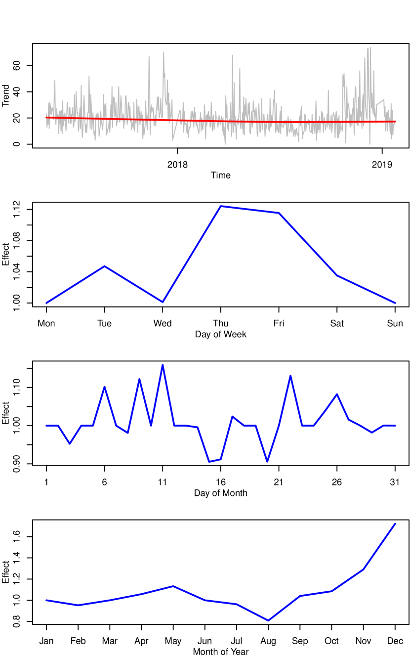
Figure 2: Structural characteristics of time series A1.

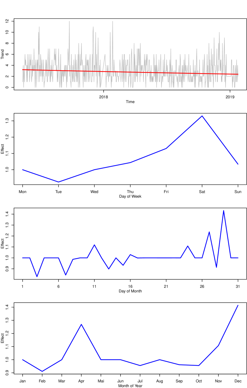
Figure 3: Structural characteristics of time series A2.

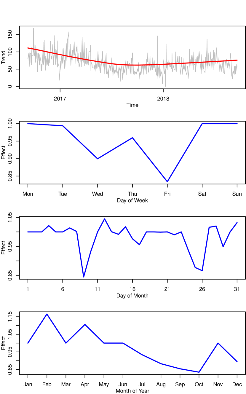
Figure 4: Structural characteristics of time series B1.

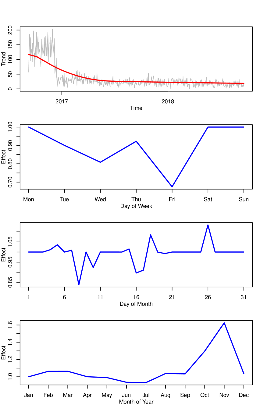
Figure 5: Structural characteristics of time series B2.

5.2 Implementation of the Models

We have implemented the models proposed in Section 4 using RStan [40], the interface between the programming languages R [34] and Stan [6]. Stan is known as a state-of-the-art platform for statistical modeling and high-performance statistical computation. In particular, Stan can be used to compute the MAP-estimate of the model parameters and also to perform full Bayesian inference via Markov chain Monte Carlo (MCMC) sampling. Hence, a few lines of Stan code, complemented by a R script to compute the matrices $\mathbf{X}$ and $\mathbf{Z}$, suffice to express our Bayesian models.

For the remainder of this section, we use the following abbreviations to identify our models: In case that the target values are assumed to be negative binomial distributed our method is abbreviated by NegBinom and in case that a normal distribution is assumed our method is denoted as Normal.

5.3 Insights on the Proposed Models

In this subsection, we illustrate how well the proposed models fit the properties of the provided real-world data. The evaluation is based on representative datasets from the above described restaurants A and B. In Section 5.3.1, the priors given by the Equations (2) – (4) are assigned to the trend functions of the considered models. Further, the standard settings specified in (12) are assigned to the tuning parameters of the models. These are our recommendations in case that the model optimization has to take place automatically and at low computational cost. In Section 5.3.2, we illustrate the superior performance of more advanced approaches for a time series associated with restaurant B.

5.3.1 Standard Approaches

At first, a representative time series A1 (compare to Section 5.1) corresponding to restaurant A is considered. In Figure 7, the model fit is visualized for Normal (5) and in Figure 7, the model fit of NegBinom is shown. The trend function is plotted in red, the seasonal function is colored green, the expected value $\mathbb{E}(\mathbf{y}|\widehat{\boldsymbol{\beta}},\widehat{\boldsymbol{\gamma}})$, see Equation (13), is drawn in dark blue and, finally, the $95\%$ prediction intervals for the components of $\mathbf{y}$ are plotted in light blue. In particular, for NegBinom, the exponential function of the trend and the season are plotted. Compared to Normal, the seasonal function of NegBinom takes small values. The reason for this is that the seasonal function acts in a multiplicative way on the trend, $\mu_{t}=\operatorname{exp}(g(\delta(t)))\operatorname{exp}(s(t))$, in NegBinom and in an additive way, $\mu_{t}=g(\delta(t))+s(t)$, in Normal.

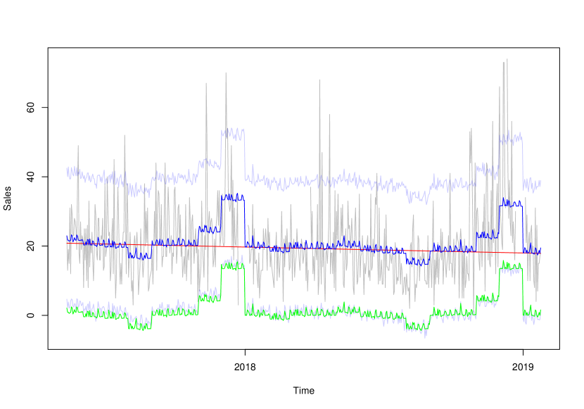
Figure 6: Model fit of Normal on the time series A1.

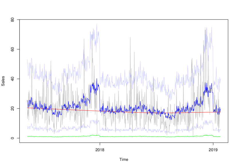
Figure 7: Model fit of NegBinom on the time series A1.

For Normal, $94.63\%$ of the observed sales lie within the $95\%$ prediction intervals. The prediction intervals of NegBinom cover $94.97\%$ of the sales. Thus, both models provide a reasonable fit of the observed time series. In Figures 9 and 9 the coefficients of the trend functions are visualized. In particular, each coefficient is plotted against the time point it has a non-zero effect on the model for the first time. Since the coefficients of the global polynomial effect the model from the beginning, different symbols are used to visualize them (a square for the intercept $\gamma_{1}$, a triangle for the coefficient $\gamma_{2}$). While Normal does not consider any significant trend changes, NegBinom detects a slight change in the second half of the year 2019. The coefficients of the seasonality functions are shown in Figures 11 and 11. While NegBinom considers more seasonal effects as significant than Normal, both models agree on the effects with the highest impact (December, November, August, Thursday, Friday, eleven-th day of month, …).

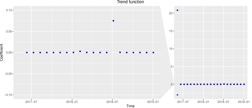
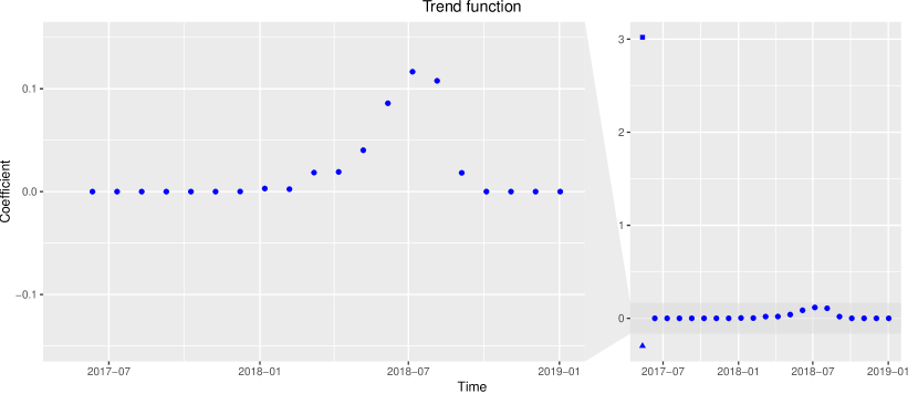
Figure 8: Coefficients of the trend function (Normal, time series A1).

Figure 9: Coefficients of the trend function (NegBinom, time series A1).

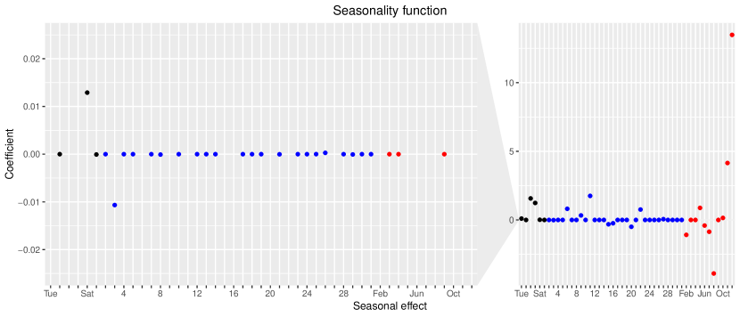
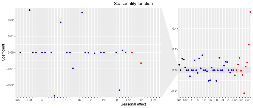
Figure 10: Coefficients of the seasonality function (Normal, time series A1).

Figure 11: Coefficients of the seasonality function (NegBinom, time series A1).

Now a representative time series B1 (compare to Section 5.1) belonging to restaurant B is considered. In Figures 13 – 17 the model fit is shown for Normal and for NegBinom The figures can be interpreted in the same way it has been done for time series A1. For Normal, $93.92157\%$ of the observed sales lie within the corresponding $95\%$ prediction intervals. The prediction intervals of NegBinom cover $95.29412\%$ of the sales.

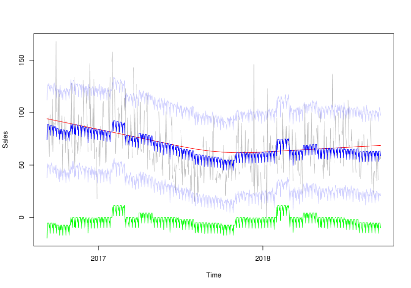
Figure 12: Model fit of Normal on the time series B1.

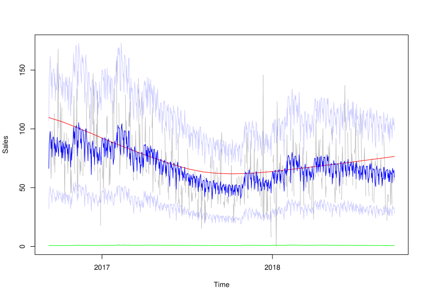
Figure 13: Model fit of NegBinom on the time series B1.

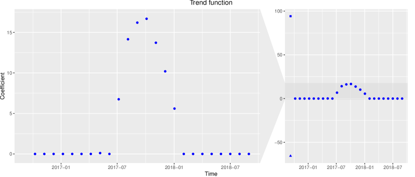
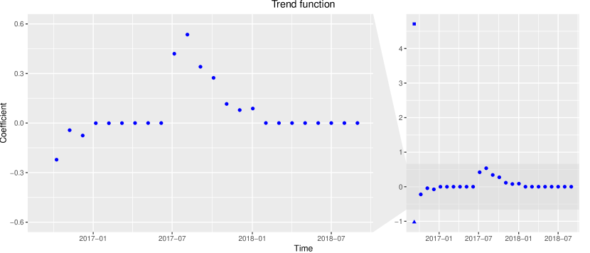
Figure 14: Coefficients of the trend function (Normal, time series B1).

Figure 15: Coefficients of the trend function (NegBinom, time series B1).

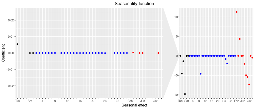
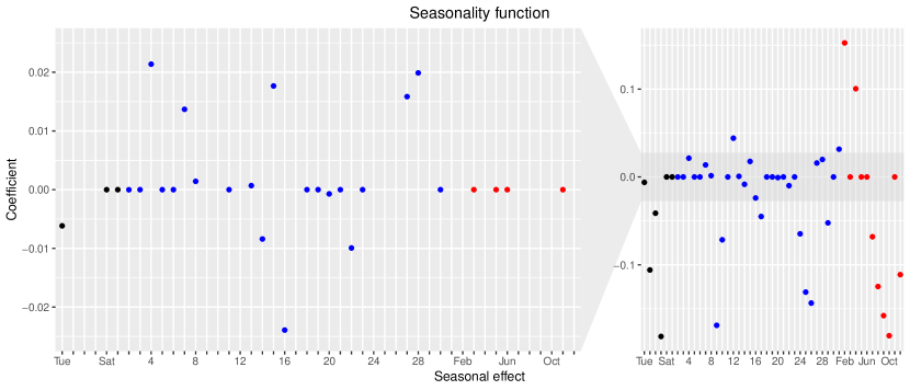
Figure 16: Coefficients of the seasonality function (Normal, time series B1).

Figure 17: Coefficients of the seasonality function (NegBinom, time series B1).

5.3.2 Advanced Approaches

In this section, the time series B2 (compare to Section 5.1) corresponding to restaurant B is considered. This time series shows a drastic trend change within a short period of time. In Figure 18, the model fit of NegBinom is visualized with different prior specifications of the trend function. We use the prior (3) – (4), that is inspired by the Bayesian Lasso, and also the horseshoe prior. In case of prior (3) – (4) the model is trained once with the standard settings (12) and once according to the step-wise cross-validation (CV) described in Section 4.5.3. The cross-validation is performed using $6$ train/test splits with the testing sets including $14$ observations, respectively. In Figures 18 and 19, we observe that the model has some serious problems in case that prior (3) – (4) is applied with the standard specification of the tuning parameters. The shrinkage of the trend coefficients is too strong, such that the trend function fails to sufficiently model the abrupt decrease at the end of 2017. If cross-validation is performed, a better model fit is obtained. However, significant trend changes are detected nearly every month which is an indication of overfitting. Due to the uniform shrinkage going along with the Lasso prior, insignificant trend changes cannot be shrunken sufficiently in order to allow for the appearance of drastic changes. Finally, an application of the horseshoe prior results in a good model fit. The trend function includes few large coefficients in absolute values to model the abrupt trend change, while most of the coefficients are equal to zero.

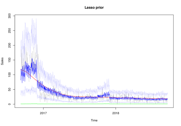
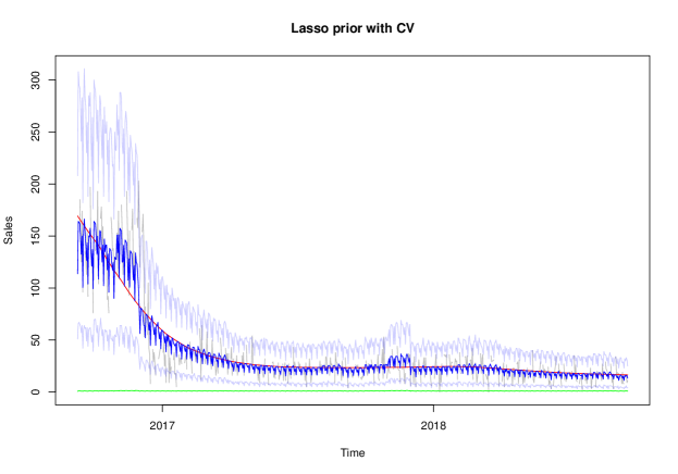
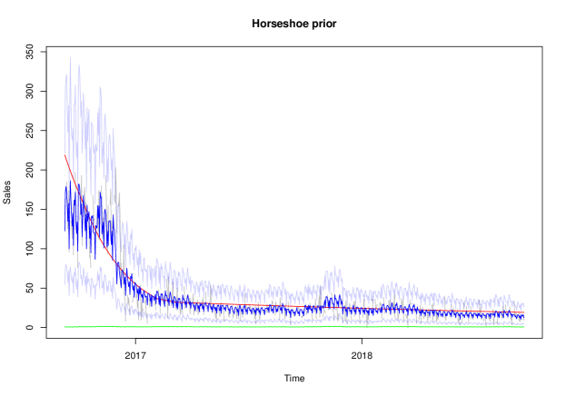
Figure 18: Model fit of NegBinom on the time series B2.

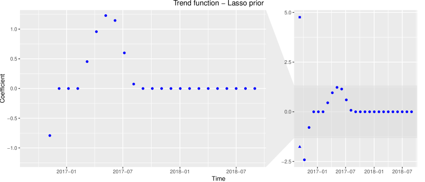
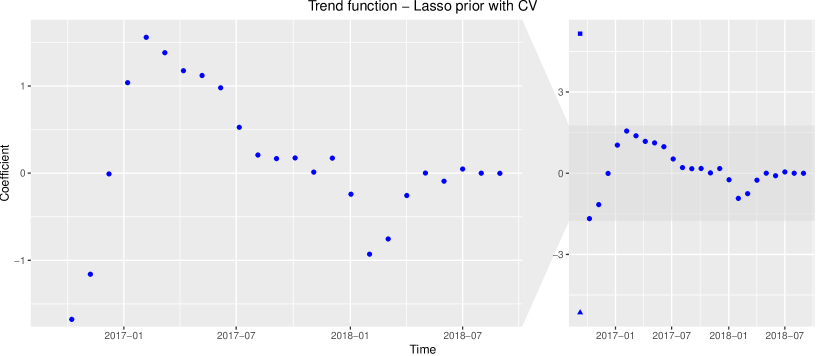
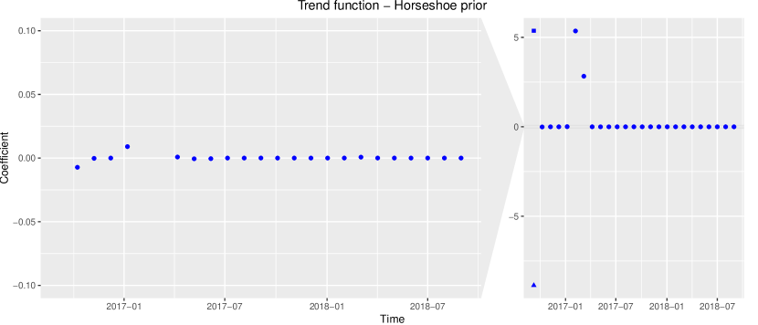
Figure 19: Trend coefficients of NegBinom on the time series B2.

5.4 Comparison Against Other Prediction Methods

In this section, the performance of our models is compared against other well-established time series forecasting approaches. The priors given by the Equations (2) – (4) are assigned to the trend functions of our models and, further, the standard settings specified in (12) for the model tuning parameters are used.

For a given time series and a given accuracy measure the performance of the considered model is evaluated using a $15$-fold cross-validation as illustrated in Figure 1. The size of the test datasets is specified as $14$.

5.4.1 Forecast Accuracy Measures

Clearly, some measures to compare the prediction quality of our approach against others are required. Let $O=\{t_{1},\ldots,t_{n}\}$ denote the set of training time points and, further, let $F=\{t_{1}^{*},\ldots,t_{p}^{*}\}$ denote the set of testing time points. Additionally, we denote the observed values with $y_{t}$ and the predicted ones with $\widehat{y}_{t}$. A review of related work, see Section 3, shows that commonly used measures for point estimates are [43, 42]:

• mean absolute deviation: $\text{MAD}=\frac{1}{p}\sum\limits_{t\in F}|y_{t}-\widehat{y}_{t}|$,

• mean squared error: $\text{MSE}=\frac{1}{p}\sum\limits_{t\in F}(y_{t}-\widehat{y}_{t})^{2}$,

• mean absolute percentage error: $\text{MAPE}=\frac{1}{p}\sum\limits_{t\in F}\left|\frac{y_{t}-\widehat{y}_{t}}{y_{t}}\right|$.

Another common measure is the mean forecast error

$$\text{MFE}=\frac{1}{p}\sum\limits_{t\in F}(y_{t}-\widehat{y}_{t}),$$

that is positive if a model tends to under-forecast and negative otherwise. Except of MAPE all up to now mentioned measures are scale dependent, i.e., the larger the $y_{t}$ the larger the error.

We compare our approach against others from the literature on several different time series, i.e., different menu items and restaurants, in order to obtain a broad comparison. Hence, it is desirable that the used prediction quality measures are scale invariant. The above mentioned scale dependent measures are important because in the restaurant industry the calculation of the nominal and safety stocks are based on these measures. In case of inferior estimates one possible encounters inventory shortages or increased food waste. For this reason, the scale dependent measures are considered in Section 5.4.3, but with the note that the aggregated values presented in this section are dominated by those time series that show the largest values on average. The scale invariant MAPE is not considered since it can not deal with zero values, i.e., $y_{t}$ must be different from zero. Some more suitable measures are the mean arctangent absolute percentage error (MAAPE), proposed by Kim and Kim [28], the weighted absolute percentage error (WAPE) [8], and the mean absolute scaled error (MASE) [24, 32]:

• $\text{MAAPE}=\frac{1}{p}\sum\limits_{t\in F}\operatorname{arctan}\left(\left|\frac{y_{t}-\widehat{y}_{t}}{y_{t}}\right|\right)$,

• $\text{WAPE}=\frac{\sum\limits_{t\in F}|y_{t}-\widehat{y}_{t}|}{\sum\limits_{t\in F}y_{t}}$,

• $\text{MASE}=\frac{\frac{1}{p}\sum\limits_{t\in F}|y_{t}-\widehat{y}_{t}|}{\operatorname{mean}(\operatorname{abs}(\mathbf{y}-\mathbf{y}_{m}))}$,

with $m\in\mathbb{N},\leavevmode\nobreak\ \mathbf{y}=(y_{t_{1}+m},\ldots,y_{t_{n}})^{\mathsf{T}}$ and $\mathbf{y}_{m}=(y_{(t_{1}+m)-m},\ldots,y_{t_{n}-m})^{\mathsf{T}}$. MAAPE can be considered as a modification of MAPE that allows for zero values since it passes the absolute percentage errors to the $\operatorname{arctan}$ function. In contrast to MAPE, WAPE weights errors by the sales volume. MASE compares the MAD of the considered forecasting model (in the testing period $F$) with the MAD of the one-step seasonal naive method with season $m$ (in the training period $O$). It should be mentioned that in Section 5.4.3 MASE is once used with $m=1$ (MASE1) and once used with $m=7$ (MASE7).

In order to evaluate the quality of the prediction intervals the following measures are helpful: prediction interval coverage probability (PICP) [38], prediction interval normalized average width (PINAW) [38], mean scaled interval score (MSIS) [15, 32]. It is desirable to have a small PINAW and a large PICP [27]. MSIS is designed to balance the relationship between PINAW and PICP. Note that in this evaluation study always $95\%$ prediction intervals are considered, since intervals with this confidence level are most commonly used in the business world [32].

5.4.2 Prediction Methods to Compare Against

Now, we briefly present the methods that we consider for comparison against our proposed model. Therefore, we adopt the selection taken by Taylor and Letham [42].

• Facebook’s prophet method. The prophet R package implements a modular regression model with interpretable parameters [42]. We discuss the model in more detail in Section 3. Within the performance comparison the model is once used with automatic season detection (prophetA) and once with yearly and weekly seasonality (prophetS).

• ARIMA. The auto.arima function returns the best ARIMA model according to the AIC or BIC value. Here, we choose the Akaike information criterion (AIC).

• Seasonal ARIMA. The auto.arima function can also be used to determine the best seasonal ARIMA (SARIMA) model. To this aim, we specify the seasonality to be weekly and, further, define the order of seasonal differencing equal to $1$. If the seasonal order is not specified, the consideration of a seasonality is decided by the auto.arima function which might also return a non-seasonal model.

• Exponential Smoothing. The ets function implements an exponential smoothing state space model. It fits a collection of exponential smoothing models and selects the best, see Hyndman et al. [25]. In this performance comparison the seasonality of the exponential smoothing model is defined to be weekly.

• TBATS. Trigonometric seasonality based on Fourier series, Box-Cox transformation, ARMA errors, Trend, and Seasonal components, see Livera et al. [30]. In this comparison study, the TBATS model is specified to learn weekly, monthly, and yearly seasonalities.

Note that all above mentioned forecasting models, except for prophet, are implemented in the forecast R package [23, 22]. We want to point out that ARIMA, SARIMA, ExpSmooth, and TBATS assume regularly spaced data points. Since the considered testing data (compare to Section 2.1 and Section 5.1) contains missing data, the missing values are linearly interpolated and subsequently rounded before fitting one of these models.

5.4.3 Evaluation

Finally, we present how our approach performs compared to the ones described above. In Tables 3 – 10 averages of the performance measures described in Section 5.4.1 are given, respectively per dataset/category. For each single time series the measures are computed based on a $15$-fold cross-validation.

Considering the results for restaurant A it can be seen that both of our models show a positive MFE for nearly all of the considered categories. This indicates, that our approach tends to under-forecast the sales numbers. While also tending to under-forecasting, the classical times series models (ARIMA, SARIMA, ExpSmooth, TBATS) show the lowest and, thus, the best MFEs. However, none of the models under comparison shows large MFEs, such that one could speak about a poor performance. In contrast to restaurant A, for restaurant B the non-standard approaches (i.e.,Normal, NegBinom, and prophet) obtain lower MFEs than the classical ones. Especially, our models show significantly lower values than all other methods under comparison.

Inspecting the MSEs and the MADs for restaurant A reveals that the proposed models often obtain the lowest errors. In case that another model performs better than ours, the differences are rather small. For restaurant B NegBinom obtains the lowest MAD and the second lowest MSE.

Switching the analysis from the scale-dependent metrics for point forecasts to the scale-invariant ones (WAPE, MAAPE, MASE) shows that our approach NegBinom shows the best results overall. For restaurant B NegBinom obtains significantly lower error values than all other considered approaches. This result is stronger than the result for the scale-dependent metrics, since the scale-invariant metrics are not dominated by the time series showing the highest number of sales.

Moreover, NegBinom always achieves the lowest mean scaled interval score. Therefore, the prediction intervals corresponding to this approach can be considered as the most useful ones. The superior performance could be explained by a good coverage probability paired with tight interval widths.

Finally, it is important to link the performance of the methods to the structural characteristics of the time series data. In Section 5.1, it is shown that the individual time series show multiple seasonalities. While, weekly, monthly, and yearly seasonal effects are observed, the strength of each of these effects differs among menu items. In principle, a method being capable of incorporating each of the mentioned seasonalities should return the best results. However, in case of limited training data one has to be careful. Allowing for too much flexibility, i.e., modeling each of the seasons, can lead to over-fitting. This may be the reason why TBATS often shows inferior results than some of the simpler forecasting approaches. On the other hand, considering only some of the seasonalities can also negatively impact the model performance. For instance, the SARIMA model, that only considers weekly seasonalities, most of the times returns worse point predictions than the simple ARIMA model. We assume that neglecting the remaining seasonalities makes it difficult to extract the true weekly effects, especially if the amount of training data is limited. Thus, we conclude that an approach which considers all of the mentioned seasonal effects, but at the same time, in terms of regularization, also penalizes the model flexibility should be preferred. This observations agree with the fact that our approach leads to the best predictions overall. Normal and NegBinom use shrinkage priors in order to automatically detect significant seasonalities and, further, to guarantee that their influence does not exceed a necessary level.

Finally, another reason for the superior performance is that all other methods somehow assume Gaussianity, while the negative binomial distribution is more appropriate to model count data. This might be the reason why NegBinom provides the most useful prediction intervals. It is likely that the use of the negative binomial distribution is a key factor. Similar findings are observed by Snyder et al. [39] who also found that models based on the negative binomial distribution give the best prediction performance concerning a forecast of the intermittent demand for slow-moving inventories, i.e., low-volume items such as auto parts. The negative binomial distribution is widely used for slow-moving inventory items, presumably because of its good performance in practice.

5.5 Evaluation of the Day of Month Effect

While it is quite intuitive that sales of menu items show weekly and yearly patterns, it is less evident that there are also effects that repeat monthly. As shown in Section 5.1 the proposed models detect monthly seasonalities within the time series data considered in this study. However, there is still the question if these effects significantly influence the model prediction accuracy. To answer this question, we have repeated the evaluation performed in Section 5.4.3 for Normal and NegBinom with the day of month effect switched off. It turns out that the usage of this explanatory variable does not have a significant influence on the average model performance, whether for Restaurant A or Restaurant B. However, a more detailed analysis shows that there are some time series where the consideration the the day of month effect leads to consistent improvements. For instance, time series A2 (compare to Section 5.1) is such a time series. In Table 11, the corresponding model accuracies are reported once with the day of month effect turned on and once with this effect turned off. We notice that the consideration of monthly patterns leads to superior accuracies. Since the additional model complexity introduced by the day of month effect has only a minor influence on the computation times, we conclude that their consideration is useful. However, we found that the model performance can only be improved for a fraction of the restaurant sales time series considered in this paper.

Measure	Normal	NegBinom	ProphetS	ProphetA	ARIMA	SARIMA	ExpSmooth	TBATS
MFE	$0.356\,873\,5$	$0.596\,802\,3$	$0.235\,714\,2$	$1.266\,542$	$0.375\,791\,7$	$0.542\,960\,7$	$0.318\,535$	$-0.059\,475\,98$
MSE	$14.494\,93$	$13.677\,89$	$13.860\,46$	$17.100\,28$	$14.168\,21$	$14.047\,31$	$12.9075$	$13.783\,54$
MAD	$2.675\,002$	$2.512\,172$	$2.644\,101$	$2.853\,282$	$2.504\,553$	$2.532\,528$	$2.457\,947$	$2.584\,678$
WAPE	$0.840\,776\,8$	$0.810\,882\,8$	$0.813\,525\,5$	$0.995\,093\,8$	$0.874\,773\,6$	$0.867\,738\,5$	$0.833\,637$	$0.836\,701\,9$
MAAPE	$0.660\,955\,4$	$0.652\,243\,7$	$0.667\,211\,7$	$0.669\,800\,3$	$0.668\,004$	$0.663\,104\,6$	$0.658\,486\,6$	$0.672\,662\,9$
MASE1	$0.815\,613\,5$	$0.750\,875\,1$	$0.813\,788\,3$	$0.865\,505\,8$	$0.745\,824$	$0.752\,779\,4$	$0.735\,345\,9$	$0.775\,929\,9$
MASE7	$0.819\,960\,6$	$0.757\,583$	$0.817\,081\,3$	$0.873\,827\,8$	$0.754\,783$	$0.763\,324\,2$	$0.745\,159\,7$	$0.782\,836\,8$
PICP	$0.926\,666\,7$	$0.935\,238\,1$	$0.925\,714\,3$	$0.903\,809\,5$	$0.944\,761\,9$	$0.938\,095\,2$	$0.942\,857\,1$	$0.939\,047\,6$
PINAW	$2.243\,829$	$1.374\,707$	$2.231\,369$	$2.435\,371$	$2.536\,522$	$2.527\,794$	$2.475\,333$	$2.290\,07$
MSIS1	$6.436\,358$	$5.458\,995$	$6.388\,803$	$7.480\,836$	$6.542\,818$	$6.503\,957$	$6.060\,836$	$6.250\,627$
MSIS7	$6.478\,731$	$5.461\,642$	$6.406\,346$	$7.549\,797$	$6.615\,704$	$6.574\,803$	$6.122\,643$	$6.295\,626$

Table 3: Performance comparison based on data from category starters collected at restaurant A.

Measure	Normal	NegBinom	ProphetS	ProphetA	ARIMA	SARIMA	ExpSmooth	TBATS
MFE	$-0.170\,222\,8$	$-0.132\,270\,3$	$-0.113\,326\,6$	$-0.188\,105$	$-0.126\,226\,9$	$-0.234\,226\,4$	$-0.149\,586$	$-0.163\,811\,2$
MSE	$8.227\,617$	$8.164\,722$	$8.070\,301$	$8.368\,138$	$8.177\,02$	$9.778\,167$	$8.195\,514$	$8.475\,017$
MAD	$2.073\,194$	$2.064\,481$	$2.066\,681$	$2.088\,12$	$2.058\,756$	$2.249\,842$	$2.053\,722$	$2.127\,686$
WAPE	$0.631\,623\,5$	$0.627\,953\,7$	$0.629\,126\,4$	$0.655\,165$	$0.632\,689\,1$	$0.688\,662\,3$	$0.630\,812\,8$	$0.654\,844\,2$
MAAPE	$0.598\,347$	$0.597\,202\,8$	$0.596\,234\,2$	$0.602\,562\,4$	$0.598\,371\,9$	$0.619\,697\,1$	$0.593\,958\,6$	$0.610\,491\,3$
MASE1	$0.767\,928\,9$	$0.765\,628\,6$	$0.768\,162\,6$	$0.783\,358\,8$	$0.771\,920\,6$	$0.837\,049\,9$	$0.769\,423\,4$	$0.799\,202\,6$
MASE7	$0.747\,929\,3$	$0.745\,485\,1$	$0.748\,203\,5$	$0.760\,870\,5$	$0.750\,405$	$0.814\,096\,1$	$0.747\,896\,6$	$0.776\,268\,1$
PICP	$0.942\,857\,1$	$0.965\,986\,4$	$0.945\,578\,2$	$0.948\,299\,3$	$0.953\,741\,5$	$0.956\,462\,6$	$0.951\,700\,7$	$0.937\,415$
PINAW	$1.329\,892$	$1.247\,955$	$1.373\,262$	$1.434\,302$	$1.471\,097$	$1.652\,499$	$1.459\,302$	$1.389\,725$
MSIS1	$5.489\,743$	$4.792\,476$	$5.343\,381$	$5.353\,174$	$5.414\,221$	$5.604\,436$	$5.324\,117$	$5.429\,39$
MSIS7	$5.317\,548$	$4.646\,741$	$5.173\,699$	$5.198\,237$	$5.251\,483$	$5.431\,977$	$5.163\,297$	$5.252\,192$

Table 4: Performance comparison based on data from category side dishes collected at restaurant A.

Measure	Normal	NegBinom	ProphetS	ProphetA	ARIMA	SARIMA	ExpSmooth	TBATS
MFE	$0.254\,977\,9$	$0.208\,541\,2$	$0.157\,583\,4$	$0.335\,764\,6$	$0.110\,206\,4$	$0.120\,323\,5$	$0.057\,879\,03$	$0.065\,183\,52$
MSE	$14.132\,85$	$13.974\,43$	$14.000\,75$	$15.679\,97$	$15.537\,79$	$16.893\,21$	$14.924\,84$	$15.281\,57$
MAD	$2.680\,936$	$2.675\,391$	$2.693\,156$	$2.799\,868$	$2.822\,731$	$2.963\,66$	$2.754\,525$	$2.810\,389$
WAPE	$0.506\,742\,5$	$0.505\,526\,6$	$0.516\,004\,5$	$0.525\,648\,9$	$0.532\,632\,7$	$0.566\,909\,3$	$0.517\,76$	$0.542\,010\,4$
MAAPE	$0.508\,667\,5$	$0.509\,770\,8$	$0.510\,729\,8$	$0.514\,779\,5$	$0.519\,441\,7$	$0.539\,119$	$0.513\,330\,4$	$0.524\,347\,8$
MASE1	$0.779\,061\,8$	$0.777\,414\,6$	$0.788\,629\,3$	$0.811\,217\,3$	$0.817\,994\,8$	$0.866\,121\,8$	$0.798\,105\,8$	$0.829\,329\,9$
MASE7	$0.785\,117\,8$	$0.783\,221\,2$	$0.794\,164$	$0.817\,364\,4$	$0.826\,642\,8$	$0.872\,208\,9$	$0.804\,663\,4$	$0.834\,852$
PICP	$0.928\,117\,9$	$0.953\,061\,2$	$0.927\,664\,4$	$0.932\,653\,1$	$0.938\,775\,5$	$0.948\,299\,3$	$0.937\,415$	$0.916\,099\,8$
PINAW	$1.211\,489$	$1.168\,017$	$1.243\,072$	$1.308\,402$	$1.368\,231$	$1.550\,877$	$1.349\,633$	$1.251\,989$
MSIS1	$5.638\,205$	$4.761\,095$	$5.666\,142$	$5.867\,706$	$5.810\,629$	$5.786\,575$	$5.571\,586$	$6.236\,446$
MSIS7	$5.695\,481$	$4.798\,255$	$5.706\,415$	$5.927\,439$	$5.876\,799$	$5.844\,616$	$5.629\,913$	$6.260\,858$

Table 5: Performance comparison based on data from category main dishes collected at restaurant A.

Measure	Normal	NegBinom	ProphetS	ProphetA	ARIMA	SARIMA	ExpSmooth	TBATS
MFE	$0.301\,701\,4$	$0.172\,607\,9$	$0.167\,661\,8$	$0.449\,995\,7$	$0.060\,239\,87$	$0.083\,688\,91$	$0.101\,739$	$0.006\,686\,447$
MSE	$5.845\,566$	$5.390\,144$	$5.795\,94$	$5.748\,678$	$5.383\,916$	$5.794\,933$	$5.461\,953$	$5.929\,645$
MAD	$1.459\,947$	$1.453\,194$	$1.513\,747$	$1.469\,039$	$1.481\,701$	$1.543\,236$	$1.482\,757$	$1.576\,512$
WAPE	$0.862\,523\,3$	$0.863\,209\,7$	$0.882\,095$	$0.844\,430\,6$	$0.880\,569$	$0.903\,767\,8$	$0.861\,877\,8$	$0.956\,689\,3$
MAAPE	$0.766\,13$	$0.770\,678\,4$	$0.789\,038\,7$	$0.785\,328\,9$	$0.782\,571$	$0.809\,677\,1$	$0.781\,639\,1$	$0.805\,851\,3$
MASE1	$0.725\,312\,6$	$0.723\,841\,6$	$0.745\,542\,1$	$0.726\,703\,9$	$0.737\,961\,4$	$0.767\,378\,6$	$0.730\,307\,2$	$0.785\,420\,5$
MASE7	$0.736\,934\,5$	$0.735\,411$	$0.757\,211\,2$	$0.738\,678\,1$	$0.749\,973\,7$	$0.779\,124\,5$	$0.742\,100\,4$	$0.798\,884\,3$
PICP	$0.953\,061\,2$	$0.968\,027\,2$	$0.950\,340\,1$	$0.955\,782\,3$	$0.963\,945\,6$	$0.968\,027\,2$	$0.964\,625\,9$	$0.957\,142\,9$
PINAW	$1.604\,493$	$1.233\,461$	$1.652\,187$	$1.714\,701$	$1.764\,03$	$1.957\,152$	$1.756\,82$	$1.663\,627$
MSIS1	$5.690\,034$	$4.539\,035$	$5.586\,051$	$5.975\,866$	$5.781\,902$	$5.966\,652$	$5.720\,662$	$5.750\,78$
MSIS7	$5.767\,792$	$4.610\,346$	$5.663\,471$	$6.055\,45$	$5.861\,913$	$6.047\,259$	$5.798\,664$	$5.821\,798$

Table 6: Performance comparison based on data from category desserts collected at restaurant A.

Measure	Normal	NegBinom	ProphetS	ProphetA	ARIMA	SARIMA	ExpSmooth	TBATS
MFE	$0.145\,918\,5$	$0.107\,464\,9$	$0.102\,482\,4$	$0.209\,968$	$-0.001\,589\,677$	$0.101\,439\,7$	$-0.002\,764\,375$	$-0.081\,451$
MSE	$12.319\,75$	$12.184\,44$	$12.044\,35$	$14.037\,06$	$12.703\,86$	$16.113\,57$	$12.900\,98$	$13.928\,04$
MAD	$1.919\,412$	$1.923\,863$	$1.948\,215$	$1.986\,885$	$1.979\,871$	$2.229\,552$	$1.9832$	$2.054\,397$
WAPE	$0.611\,392\,3$	$0.612\,700\,4$	$0.622\,371\,8$	$0.622\,501\,9$	$0.632\,912\,4$	$0.713\,677\,6$	$0.630\,206$	$0.644\,382\,5$
MAAPE	$0.586\,474\,4$	$0.587\,483\,7$	$0.594\,548\,9$	$0.591\,144\,1$	$0.595\,445\,4$	$0.634\,746\,4$	$0.595\,874\,4$	$0.604\,886\,5$
MASE1	$0.749\,677\,5$	$0.750\,319\,9$	$0.763\,517\,7$	$0.767\,958\,7$	$0.773\,569\,5$	$0.873\,226\,4$	$0.772\,418\,4$	$0.790\,804\,9$
MASE7	$0.746\,573\,8$	$0.747\,156\,2$	$0.760\,514\,7$	$0.764\,459\,2$	$0.770\,550\,9$	$0.870\,281\,3$	$0.768\,815$	$0.786\,875\,9$
PICP	$0.940\,773\,8$	$0.967\,261\,9$	$0.937\,797\,6$	$0.945\,238\,1$	$0.953\,273\,8$	$0.956\,547\,6$	$0.950\,595\,2$	$0.938\,988\,1$
PINAW	$1.227\,338$	$1.161\,172$	$1.265\,572$	$1.321\,901$	$1.373\,465$	$1.641\,748$	$1.350\,288$	$1.278\,358$
MSIS1	$5.247\,69$	$4.496\,459$	$5.207\,521$	$5.471\,71$	$5.317\,956$	$5.975\,563$	$5.257\,222$	$5.323\,224$
MSIS7	$5.206\,548$	$4.463\,839$	$5.175\,618$	$5.427\,682$	$5.284\,129$	$5.941\,989$	$5.219\,886$	$5.284\,743$

Table 7: Performance comparison based on data from category snacks collected at restaurant A.

Measure	Normal	NegBinom	ProphetS	ProphetA	ARIMA	SARIMA	ExpSmooth	TBATS
MFE	$0.392\,624\,2$	$0.390\,011\,7$	$0.324\,201\,1$	$0.567\,100\,3$	$-0.034\,434\,36$	$0.002\,148\,72$	$0.062\,741\,1$	$27.114\,15$
MSE	$84.781\,69$	$85.736\,86$	$86.012\,01$	$102.7643$	$122.2761$	$101.1332$	$97.739\,78$	$1\,124\,662.000$
MAD	$4.518\,726$	$4.525\,069$	$4.657\,049$	$4.788\,381$	$5.081\,013$	$5.086\,446$	$4.680\,459$	$40.096\,06$
WAPE	$0.738\,744$	$0.733\,458\,3$	$0.812\,321\,5$	$0.750\,129$	$0.762\,844\,7$	$0.823\,97$	$0.745\,132\,1$	$12.047\,72$
MAAPE	$0.633\,002\,7$	$0.629\,094\,8$	$0.646\,136\,5$	$0.640\,201\,6$	$0.650\,253\,2$	$0.680\,001\,5$	$0.638\,426\,4$	$0.658\,268$
MASE1	$0.742\,323\,5$	$0.739\,836\,9$	$0.807\,179\,5$	$0.765\,024$	$0.782\,678\,2$	$0.858\,448\,5$	$0.756\,075\,2$	$15.882\,04$
MASE7	$0.744\,210\,1$	$0.741\,676\,5$	$0.813\,040\,3$	$0.767\,487\,5$	$0.786\,083\,3$	$0.860\,881\,3$	$0.758\,205\,8$	$18.416\,93$
PICP	$0.941\,798\,9$	$0.957\,848\,3$	$0.936\,507\,9$	$0.943\,739$	$0.950\,264\,6$	$0.954\,673\,7$	$0.951\,851\,9$	$0.929\,276\,9$
PINAW	$1.406\,165$	$1.226\,277$	$1.445\,418$	$1.523\,252$	$1.593\,37$	$1.846\,701$	$1.558\,657$	$1.458\,473$
MSIS1	$5.972\,293$	$4.947\,007$	$7.494\,552$	$6.200\,472$	$6.128\,499$	$6.541\,344$	$5.964\,309$	$609.6048$
MSIS7	$5.980\,117$	$4.956\,01$	$7.623\,279$	$6.216\,109$	$6.145\,332$	$6.552\,81$	$5.974\,91$	$710.8797$

Table 8: Performance comparison based on data from category alcoholic beverages collected at restaurant A.

Measure	Normal	NegBinom	ProphetS	ProphetA	ARIMA	SARIMA	ExpSmooth	TBATS
MFE	$0.167\,270\,3$	$0.127\,675\,3$	$0.112\,701\,7$	$0.108\,703\,2$	$0.033\,135\,73$	$0.027\,317\,43$	$0.007\,350\,705$	$0.076\,764\,29$
MSE	$8.639\,13$	$8.603\,087$	$8.931\,199$	$9.345\,957$	$9.309\,124$	$10.800\,58$	$9.241\,184$	$9.746\,363$
MAD	$2.017\,433$	$2.013\,264$	$2.063\,239$	$2.079\,467$	$2.091\,063$	$2.241\,962$	$2.081\,28$	$2.134\,773$
WAPE	$0.755\,681\,6$	$0.753\,993\,8$	$0.774\,132\,6$	$0.778\,719\,4$	$0.771\,632\,2$	$0.834\,248\,3$	$0.763\,579\,9$	$0.784\,150\,2$
MAAPE	$0.683\,730\,5$	$0.683\,552\,9$	$0.699\,298\,4$	$0.691\,011\,4$	$0.694\,889\,6$	$0.727\,704\,5$	$0.694\,035\,5$	$0.706\,046\,1$
MASE1	$0.761\,851\,5$	$0.760\,354\,1$	$0.779\,960\,6$	$0.780\,931\,1$	$0.784\,893\,4$	$0.845\,642\,1$	$0.779\,700\,6$	$0.799\,839\,3$
MASE7	$0.767\,802\,9$	$0.766\,256\,3$	$0.785\,819\,4$	$0.786\,934\,5$	$0.790\,995\,8$	$0.852\,136\,7$	$0.785\,407\,7$	$0.806\,114\,4$
PICP	$0.940\,327\,4$	$0.967\,261\,9$	$0.937\,053\,6$	$0.947\,321\,4$	$0.949\,702\,4$	$0.951\,785\,7$	$0.949\,553\,6$	$0.934\,821\,4$
PINAW	$1.414\,125$	$1.227\,556$	$1.457\,502$	$1.528\,093$	$1.556\,707$	$1.792\,123$	$1.555\,826$	$1.485\,368$
MSIS1	$5.724\,734$	$4.522\,523$	$5.716\,661$	$5.924\,839$	$5.837\,592$	$6.210\,902$	$5.765\,902$	$5.969\,027$
MSIS7	$5.769\,615$	$4.558\,809$	$5.764\,296$	$5.971\,963$	$5.886\,676$	$6.259\,513$	$5.811\,79$	$6.019\,709$

Table 9: Performance comparison based on data from category non-alcoholic beverages collected at restaurant A.

Measure	Normal	NegBinom	ProphetS	ProphetA	ARIMA	SARIMA	ExpSmooth	TBATS
MFE	$-0.734\,887\,3$	$0.480\,969\,5$	$-2.863\,709$	$-3.589\,308$	$-5.061\,448$	$-9.297\,509$	$-5.191\,48$	$-7.497\,736$
MSE	$37\,364.71$	$36\,975.5$	$40\,162.94$	$37\,331.88$	$36\,956.45$	$49\,030.34$	$38\,858.29$	$39\,497.44$
MAD	$44.039\,61$	$41.1646$	$47.0454$	$44.489\,96$	$45.176\,81$	$49.545\,53$	$45.311\,06$	$46.757\,94$
WAPE	$0.903\,118\,4$	$0.736\,399\,4$	$0.953\,720\,9$	$0.815\,977\,4$	$0.810\,492\,9$	$0.937\,306\,8$	$0.837\,517$	$0.854\,749\,1$
MAAPE	$0.614\,194\,7$	$0.580\,098\,2$	$0.640\,587\,7$	$0.601\,739\,1$	$0.614\,976\,9$	$0.588\,270\,2$	$0.620\,801\,1$	$0.621\,093\,1$
MASE1	$0.923\,871$	$0.839\,521\,3$	$0.985\,415\,3$	$0.839\,669\,9$	$0.857\,164\,9$	$0.899\,404\,3$	$0.889\,970\,5$	$0.893\,937\,5$
MASE7	$0.937\,728\,3$	$0.846\,649\,9$	$0.998\,807\,8$	$0.851\,344\,4$	$0.870\,847\,7$	$0.916\,010\,5$	$0.900\,173\,5$	$0.905\,116\,1$
PICP	$0.912\,698\,4$	$0.91$	$0.893\,650\,8$	$0.943\,015\,9$	$0.940\,634\,9$	$0.939\,206\,3$	$0.947\,936\,5$	$0.914\,127$
PINAW	$2.422\,543$	$1.653\,406$	$2.513\,839$	$2.657\,171$	$2.584\,516$	$2.964\,648$	$98.260\,26$	$2.360\,085$
MSIS1	$8.287\,771$	$6.619\,74$	$9.709\,142$	$7.497\,961$	$7.540\,283$	$7.825\,233$	$404.4657$	$8.099\,009$
MSIS7	$8.497\,117$	$6.793\,278$	$9.923\,391$	$7.677\,196$	$7.749\,66$	$8.051\,975$	$438.2527$	$8.238\,03$

Table 10: Performance comparison based on data collected at restaurant B.

Measure	Normal without monthly effect	Normal with monthly effect	NegBinom without monthly effect	NegBinom with monthly effect
MFE	$-0.003\,631\,506$	$0.001\,658\,735$	$-0.011\,191\,95$	$-0.011\,752\,46$
MSE	$4.057\,998$	$3.986\,821$	$4.006\,592$	$3.889\,596$
MAD	$1.608\,995$	$1.594\,948$	$1.601\,26$	$1.580\,636$
WAPE	$0.596\,257\,1$	$0.591\,144$	$0.593\,831\,5$	$0.586\,106\,1$
MAAPE	$0.592\,699\,6$	$0.589\,821\,3$	$0.591\,643\,6$	$0.587\,677\,6$
MASE1	$0.704\,205\,7$	$0.698\,044\,9$	$0.700\,886$	$0.691\,809\,1$
MASE7	$0.741\,564\,6$	$0.735\,096\,7$	$0.737\,999\,3$	$0.728\,469\,7$
PICP	$0.957\,142\,9$	$0.95$	$0.969\,047\,6$	$0.969\,047\,6$
PINAW	$1.260\,362$	$1.220\,559$	$1.133\,475$	$1.108\,623$
MSIS1	$4.526\,777$	$4.429\,215$	$3.812\,071$	$3.740\,714$
MSIS7	$4.763\,454$	$4.659\,933$	$4.011\,587$	$3.936\,838$

Table 11: Performance evaluation of the day of month effect for time series A2.

6 Conclusion & Future Work

In this work, a new approach for predicting future sales of menu items in restaurants and staff canteens was proposed. In particular, two Bayesian generalized additive models were presented. The first one assumes future sales to be normally distributed, while the second one uses the more appropriate negative Binomial distribution. Both approaches use shrinkage priors to automatically learn significant multiple seasonal effects and trend changes. The features learned by the models have a straightforward human interpretation which helps potential users to create the necessary trust and confidence in the methodology. The performance of our approach was extensively evaluated and compared to other well-established forecasting methods. Basis of the analysis were two data sets retrieved from (electronic) Point of Sales (POS) systems collected at a restaurant and a staff canteen. The evaluations show that our approach often provides the best and most robust point predictions overall. Moreover, the prediction intervals of our model with the negative Binomial distribution are notably more accurate than the ones obtained by the other methods.

Currently, our approach only takes account of POS data. This makes it universally applicable, but also limits the prediction quality that can be achieved. In future work, we plan to enrich the data source by weather data, information regarding special events and holidays, and, last but not least, expert knowledge of restaurant managers. Additionally, we want to extend our approach such that it can also predict on hourly basis. Accurate sales predictions on hourly basis will allow an optimization of workforce planning.

References

- TON [2018] Environmental impacts of food waste: Learnings and challenges from a case study on UK. Waste Management, 76:744–766, 2018. ISSN 0956-053X. doi:10.1016/j.wasman.2018.03.032.
- NRA [2019] 2019 restaurant industry factbook, 2019. URL https://restaurant.org/Downloads/PDFs/Research/SOI/restaurant_industry_fact_sheet_2019.pdf. [Online; accessed 29-Oct-2019].
- ReF [2019] Restaurant food waste action guide, 2019. URL https://www.refed.com/downloads/Restaurant_Guide_Web.pdf. [Online; accessed 29-Oct-2019].
- Bhattacharya et al. [2015] Anirban Bhattacharya, Debdeep Pati, Natesh S. Pillai, and David B. Dunson. Dirichlet–Laplace priors for optimal shrinkage. Journal of the American Statistical Association, 110(512):1479–1490, 2015. doi:10.1080/01621459.2014.960967.
- Bujisic et al. [2017] Milos Bujisic, Vanja Bogicevic, and H. G. Parsa. The effect of weather factors on restaurant sales. Journal of Foodservice Business Research, 20(3):350–370, May 2017. ISSN 1537-8020, 1537-8039. doi:10.1080/15378020.2016.1209723.
- Carpenter et al. [2017] Bob Carpenter, Andrew Gelman, Matthew Hoffman, Daniel Lee, Ben Goodrich, Michael Betancourt, Marcus Brubaker, Jiqiang Guo, Peter Li, and Allen Riddell. Stan: A probabilistic programming language. Journal of Statistical Software, Articles, 76(1):1–32, 2017. ISSN 1548-7660. doi:10.18637/jss.v076.i01.
- Carvalho et al. [2010] Carlos M. Carvalho, Nicholas G. Polson, and James G. Scott. The horseshoe estimator for sparse signals. Biometrika, 97(2):465–480, 2010. doi:10.2307/25734098.
- Chase [1995] J. W. Chase. Measuring forecast accuracy. The Journal of Business Forecasting Methods & Systems, 14:2, 1995.
- Coleman-Jensen et al. [2019] Alisha Coleman-Jensen, Matthew P. Rabbitt, Christian A. Gregory, and Anita Singh. Household food security in the United States in 2018, err-270,. U.S. Department of Agriculture, Economic Research Service, September 2019. URL https://www.ers.usda.gov/webdocs/publications/94849/err-270.pdf?v=963.1.
- Conway and Maxwell [1962] R. W. Conway and W. L. Maxwell. A queuing model with state dependent service rates. Journal of Industrial Engineering, 12:132–136, 1962.
- Cranage and Andrew [1992] David A. Cranage and William P. Andrew. A comparison of time series and econometric models for forecasting restaurant sales. International Journal of Hospitality Management, 11(2):129–142, 1992. doi:10.1016/0278-4319(92)90006-H.
- Fahrmeir et al. [2013] Ludwig Fahrmeir, Thomas Kneib, Stefan Lang, and Brian Marx. Regression - Models, Methods and Applications. Springer, Berlin Heidelberg, 2013. doi:10.1007/978-3-642-34333-9.
- Forst [1992] Frank G. Forst. Forecasting restaurant sales using multiple regression and Box-Jenkins analysis. Journal of Applied Business Research, 8(2):15–19, 1992. doi:10.19030/jabr.v8i2.6157.
- Gelman [2019] Andrew Gelman. Prior choice recommendations. https://github.com/stan-dev/stan/wiki/Prior-Choice-Recommendations, 2019. [Online; accessed 03-Nov-2019].
- Gneiting and Raftery [2007] Tilmann Gneiting and Adrian E Raftery. Strictly proper scoring rules, prediction, and estimation. Journal of the American Statistical Association, 102(477):359–378, 2007. doi:10.1198/016214506000001437.
- Gould et al. [2008] Phillip G. Gould, Anne B. Koehler, J. Keith Ord, Ralph D. Snyder, Rob J. Hyndman, and Farshid Vahid-Araghi. Forecasting time series with multiple seasonal patterns. European Journal of Operational Research, 191(1):207–222, 2008. ISSN 0377-2217. doi:10.1016/j.ejor.2007.08.024.
- Hastie and Tibshirani [1987] Trevor Hastie and Robert Tibshirani. Generalized additive models: Some applications. Journal of the American Statistical Association, 82(398):371–386, 1987. ISSN 01621459. doi:10.2307/2289439.
- Hickey and Ozbay [2014] Michael E. Hickey and Gulnihal Ozbay. Food waste in the United States: A contributing factor toward environmental instability. Frontiers in Environmental Science, 2:51, 2014. ISSN 2296-665X. doi:10.3389/fenvs.2014.00051.
- Hilbe et al. [2017] Joseph M. Hilbe, Rafael S. de Souza, and Emille E. O. Ishida. Bayesian Models for Astrophysical Data: Using R, JAGS, Python, and Stan. Cambridge University Press, 2017. doi:10.1017/CBO9781316459515.
- Holt [2004] Charles C. Holt. Forecasting seasonals and trends by exponentially weighted moving averages. International Journal of Forecasting, 20(1):5–10, 2004. doi:10.1016/j.ijforecast.2003.09.015.
- Hu et al. [2004] Clark Hu, Ming Chen, and Shiang-Lih Chen McCain. Forecasting in short-term planning and management for a casino buffet restaurant. Journal of Travel & Tourism Marketing, 16(2-3):79–98, July 2004. doi:10.1300/J073v16n02_07.
- Hyndman et al. [2019] Rob Hyndman, George Athanasopoulos, Christoph Bergmeir, Gabriel Caceres, Leanne Chhay, Mitchell O’Hara-Wild, Fotios Petropoulos, Slava Razbash, Earo Wang, and Farah Yasmeen. forecast: Forecasting functions for time series and linear models, 2019. URL http://pkg.robjhyndman.com/forecast. R package version 8.9.
- Hyndman and Khandakar [2008] Rob J Hyndman and Yeasmin Khandakar. Automatic time series forecasting: The forecast package for R. Journal of Statistical Software, 26(3):1–22, 2008. URL http://www.jstatsoft.org/article/view/v027i03.
- Hyndman and Koehler [2006] Rob J. Hyndman and Anne B. Koehler. Another look at measures of forecast accuracy. International Journal of Forecasting, 22(4):679–688, 2006. ISSN 0169-2070. doi:10.1016/j.ijforecast.2006.03.001.
- Hyndman et al. [2002] Rob J Hyndman, Anne B Koehler, Ralph D Snyder, and Simone Grose. A state space framework for automatic forecasting using exponential smoothing methods. International Journal of Forecasting, 18(3):439–454, 2002. ISSN 0169-2070. doi:10.1016/S0169-2070(01)00110-8.
- Kaneko and Yada [2016] Y. Kaneko and K. Yada. A deep learning approach for the prediction of retail store sales. In 2016 IEEE 16th International Conference on Data Mining Workshops (ICDMW), pages 531–537, Dec 2016. doi:10.1109/ICDMW.2016.0082.
- Khosravi et al. [2010] Abbas Khosravi, Saeid Nahavandi, and Doug Creighton. A prediction interval-based approach to determine optimal structures of neural network metamodels. Expert Systems with Applications, 37(3):2377–2387, 2010. ISSN 0957-4174. doi:10.1016/j.eswa.2009.07.059.
- Kim and Kim [2016] Sungil Kim and Heeyoung Kim. A new metric of absolute percentage error for intermittent demand forecasts. International Journal of Forecasting, 32(3):669–679, 2016. ISSN 0169-2070. doi:10.1016/j.ijforecast.2015.12.003.
- Lasek et al. [2016] Agnieszka Lasek, Nick Cercone, and Jim Saunders. Restaurant sales and customer demand forecasting: Literature survey and categorization of methods. In Alberto Leon-Garcia, Radim Lenort, David Holman, David Staš, Veronika Krutilova, Pavel Wicher, Dagmar Cagáňová, Daniela Špirková, Julius Golej, and Kim Nguyen, editors, Smart City 360, pages 479–491, Cham, 2016. Springer International Publishing. ISBN 978-3-319-33681-7. doi:10.1007/978-3-319-33681-7_40.
- Livera et al. [2011] Alysha M. De Livera, Rob J. Hyndman, and Ralph D. Snyder. Forecasting time series with complex seasonal patterns using exponential smoothing. Journal of the American Statistical Association, 106(496):1513–1527, 2011. doi:10.1198/jasa.2011.tm09771.
- Makalic and Schmidt [2016] E. Makalic and D. F. Schmidt. A simple sampler for the horseshoe estimator. IEEE Signal Processing Letters, 23(1):179–182, 2016. doi:10.1109/LSP.2015.2503725.
- Makridakis et al. [2020] Spyros Makridakis, Evangelos Spiliotis, and Vassilios Assimakopoulos. The M4 competition: 100,000 time series and 61 forecasting methods. International Journal of Forecasting, 36(1):54–74, 2020. ISSN 0169-2070. doi:10.1016/j.ijforecast.2019.04.014. M4 Competition.
- Park and Casella [2008] Trevor Park and George Casella. The Bayesian Lasso. Journal of the American Statistical Association, 103(482):681–686, 2008. doi:10.1198/016214508000000337.
- R Core Team [2019] R Core Team. R: A Language and Environment for Statistical Computing. R Foundation for Statistical Computing, Vienna, Austria, 2019. URL https://www.R-project.org.
- Reynolds et al. [2013] Dennis Reynolds, Imran Rahman, and William Balinbin. Econometric modeling of the U.S. restaurant industry. International Journal of Hospitality Management, 34:317–323, September 2013. doi:10.1016/j.ijhm.2013.04.003.
- Rockova and George [2018] Veronika Rockova and Edward I. George. The spike-and-slab LASSO. Journal of the American Statistical Association, 113(521):431–444, 2018. doi:10.1080/01621459.2016.1260469.
- Ryu and Sanchez [2003] Kisang Ryu and Alfonso Sanchez. The evaluation of forecasting methods at an institutional foodservice dining facility. The Journal of Hospitality Financial Management, 11(1):27–45, 2003.
- Shen et al. [2018] Yanxia Shen, Xu Wang, and Jie Chen. Wind power forecasting using multi-objective evolutionary algorithms for wavelet neural network-optimized prediction intervals. Applied Sciences, 8:185, 2018.
- Snyder et al. [2012] Ralph D. Snyder, J. Keith Ord, and Adrian Beaumont. Forecasting the intermittent demand for slow-moving inventories: A modelling approach. International Journal of Forecasting, 28(2):485–496, 2012. ISSN 0169-2070. doi:10.1016/j.ijforecast.2011.03.009.
- Stan Development Team [2018] Stan Development Team. RStan: The R interface to Stan, 2018. URL http://mc-stan.org/. R package version 2.18.2.
- Tanizaki et al. [2019] Takashi Tanizaki, Tomohiro Hoshino, Takeshi Shimmura, and Takeshi Takenaka. Demand forecasting in restaurants using machine learning and statistical analysis. Procedia CIRP, 79:679–683, 2019. ISSN 2212-8271. doi:10.1016/j.procir.2019.02.042. 12th CIRP Conference on Intelligent Computation in Manufacturing Engineering, 18-20 July 2018, Gulf of Naples, Italy.
- Taylor and Letham [2018] Sean J. Taylor and Benjamin Letham. Forecasting at scale. The American Statistician, 72(1):37–45, 2018. doi:10.1080/00031305.2017.1380080.
- Xinliang and Dandan [2017] Liu Xinliang and Sun Dandan. University restaurant sales forecast based on BP neural network – in Shanghai Jiao Tong university case. In Ying Tan, Hideyuki Takagi, Yuhui Shi, and Ben Niu, editors, Advances in Swarm Intelligence, pages 338–347, Cham, 2017. Springer International Publishing. ISBN 978-3-319-61833-3. doi:10.1007/978-3-319-61833-3_36.