Impurity resonance effects in graphene vs impurity location, concentration and sublattice occupation

Abstract

Unique electronic band structure of graphene with its semi-metallic features near the charge neutrality point is sensitive to impurity effects. Using the Lifshitz and Anderson impurity models, we study in detail the disorder induced spectral phenomena in the electronic band structure of graphene, namely, the formation of resonances, quasi-gaps, bound states, impurity sub-bands, and their overall impact on the electronic band restructuring and the associated Mott-like metal-insulator transitions. We perform systematic analytical and numerical study for realistic impurities, both substitutional and adsorbed, focusing on those effects that stem from the impurity adatoms locations (top, bridge, and hollow positions), concentration, host sublattice occupation, perturbation strengths, etc. Possible experimental and practical implications are discussed as well.

I Introduction

Graphene is the first two-dimensional crystal possessing linear dispersion of low energy electronic states. Therefore they can be described by an effective Dirac equation for 2D massless fermions. However, in experiments long-range Coulomb scattering Adam et al. (2007); Swartz et al. (2013); Jia et al. (2015); Chandni et al. (2015) off charged adatoms, as well, short-range scattering off the non-charged impurities can strongly affect graphene’s transport properties. A representative example of a short-range impurity is vacancy that is predicted to give rise to zero energy resonance states in graphene Pereira et al. (2006, 2008); Nanda et al. (2012). Due to the small density of states (DOS) at low energy, graphene is especially very sensitive to such induced resonant states Stauber et al. (2007); Ferreira et al. (2011); Monteverde et al. (2010); Robinson et al. (2008); Lee et al. (2019). Another source for these states are various substitutional impurities Basko (2008); Wehling et al. (2007a); Pereira et al. (2008); Skrypnyk and Loktev (2006) or adsorbates in graphene. The latter have been studied for specific adatoms by explicit tight-binding and density-functional theory calculations, see for example Ihnatsenka and Kirczenow (2011); Wehling et al. (2010a, b, 2007b); Farjam et al. (2011); Gmitra et al. (2013); Zollner et al. (2016); Frank et al. (2017), It was also realized by the basic symmetry analysis that the adsorption position of an adatom plays an important role for the resonance scattering mechanism Ruiz-Tijerina and da Silva (2016); Uchoa et al. (2014); Weeks et al. (2011a); Duffy et al. (2016); Irmer et al. (2018). For example, it was established that the $s$-orbital of an adatom in hollow position is effectively decoupled from the electronic states of graphene Ruiz-Tijerina and da Silva (2016) so that resonance scattering of such an orbital is strongly suppressed. Generally, this sensitivity to impurity location can be related to the specifics of graphene lattice that owns two sublattices, each of them with no local inversion symmetry, the same that defines the most notable feature of pure graphene’s spectrum, its Dirac points.

Our work aims to provide extended, self-contained and systematic study of spectral properties of graphene in the presence of impurity disorder and the underlying onset of the Mott-like metal insulator transitions considering dependencies on impurity concentration, their position type (top, bridge, hollow), sublattice occupation asymmetry and so on, and connect those with some previous theoretical studies available in the literature. We consider two models; Lifshitz isotopic model Lifshitz et al. (1988), and Anderson hybrid model Anderson (1961). As will be shown, distribution of impurities position with respect to the host sublattices can create an occupational asymmetry. The spectral properties of graphene (resonances, quasi-gaps, mobility edges, impurity subgaps, etc.) are very sensitive, besides the total impurity concentration, also to such partial occupation asymmetries.

The paper is organized as follows, Section II presents a short introduction into the formulation of the tight-binding model and Green’s functions formalism. Then in Sec. III we consider the simpler Lifshitz isotopic model of impurity perturbation and demonstrates certain specific effects appearing there even in the absence of impurity resonances. Those resonances in their general form are further investigated in Sec. IV within the scope of Anderson’s hybrid model, while Secs. V and VI analyzes their particular realizations for different types of impurity positions and their sublattice occupations. Finally, a discussion of the obtained results and their possible applications are given in Sec. VII. Some more technical details of calculations, such as the restructured spectrum to higher order, are provided in Appendices A and B.

II Model and Green functions

We model the unperturbed graphene in terms of the tight-binding Hamiltonian:

$$H_{0}=t\sum_{\langle{\bf n}_{1},{\bf n}_{2}\rangle}\left(b_{{\bf n}_{1}}^{\dagger}b_{{\bf n}_{2}}^{\phantom{\dagger}}+h.c.\right)\,,$$ (1)

where the carbon $2p_{z}$-atomic level is chosen as the energy reference. Hoppings, parameterized by the amplitude $t$, connect nearest-neighbor graphene sites as symbolically indicated by $\langle{\bf n}_{1},{\bf n}_{2}\rangle$. Here and below ${\bf n}_{1}$ stands for a site from sublattice-type 1 (A-sublattice), and ${\bf n}_{2}$ for sublattice-type 2 (B-sublattice), see Fig. 1, in generic case we use symbol ${\bf n}_{j}$. Here and in what follows we do not consider explicitly the electron spin degrees of freedom assuming purely spin-diagonal hoppings so that the on-site energies and all the observable quantities are understood per single spin projection.

The Hamiltonian $H_{0}$ is routinely diagonalized passing from the direct-space representation, through the local atomic Fermi operators $b_{{\bf n}_{j}}^{(\dagger)}$, to the corresponding Bloch band representation:

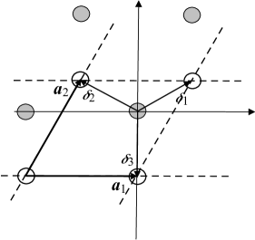
Figure 1: Graphene lattice structure with $t$-hopping links along the nearest-neighbor vectors ${\boldsymbol{\delta}}_{1,2,3}$ connecting type-1/sublattice-A (grey), and type-2/sublattice-B (white) carbon sites. Dashed lines mark the unit cells formed by the elementary translation vectors ${\bf a}_{1,2}$.

$$H_{0}=\sum_{{\bf k}}\varepsilon_{\bf k}\left(\beta_{+,{\bf k}}^{\dagger}\beta_{+,{\bf k}}^{\phantom{\dagger}}-\beta_{-,{\bf k}}^{\dagger}\beta_{-,{\bf k}}^{\phantom{\dagger}}\right).$$ (2)

Here the eigenenergies $\varepsilon_{\bf k}$, and the band operators $\beta_{\pm,{\bf k}}^{(\dagger)}$ are labeled by the wave-vector ${\bf k}$ that belongs to the first Brillouin zone (BZ) spanned by the reciprocal basis vectors ${\bf b}_{1,2}$, i.e. ${\bf b}_{j}\cdot{\bf a}_{j^{\prime}}=2\pi\delta_{j,j^{\prime}}$, see Fig. 2. Moreover, the sign subscript $\pm$ refers to the conduction and valence bands, respectively. The corresponding energy dispersion laws, $\pm\varepsilon_{\bf k}=\pm t|\gamma_{\bf k}|$, follow from the hopping factor:

$$\gamma_{\bf k}=\sum_{\boldsymbol{\delta}}{\rm e}^{i{\bf k}\cdot\boldsymbol{\delta}}=2\cos\frac{k_{x}}{2}{\rm e}^{ik_{y}/2\sqrt{3}}+{\rm e}^{-ik_{y}/\sqrt{3}}\,,$$ (3)

(in what follows the quasi-momenta are measured in units of the inverse graphene lattice constant $a^{-1}=|{\bf a}_{1,2}|^{-1}=|\sqrt{3}\,\boldsymbol{\delta}|^{-1}$).

The band, and the lattice (local atomic) operators are related via the Fourier transformation:

$$b_{{\bf n}_{j}}=\frac{1}{\sqrt{2N}}\sum_{\bf k}{\rm e}^{i\phi_{{\bf n}_{j},{\bf k}}}\left(\beta_{+,{\bf k}}-(-1)^{j}\beta_{-,{\bf k}}\right),$$ (4)

where $N$ represents the number of unit cells, and the hopping phase reads:

$$\phi_{{\bf n}_{j},{\bf k}}={\bf k}\cdot{\bf n}_{j}-\frac{(-1)^{j}}{2}\arg\gamma_{\bf k}\,.$$ (5)

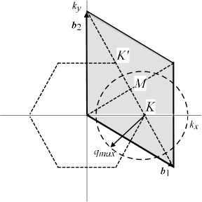
Figure 2: Brillouin zone of graphene (shadowed rhombus) with the corresponding Dirac points $\mathbf{K}$ and $\mathbf{K}^{\prime}$, and the associated reciprocal lattice vectors $\boldsymbol{b}_{1,2}$. An effective "half" of the Brillouin zone centered at ${\bf K}$ point (dashed circle) with the cut off momentum $q_{max}$ hosts the same number of states as half of the rhombus at ${\bf K}$ valley.

Near the Dirac points, ${\bf K}=(4\pi/3,0)$ or ${\bf K}^{\prime}=(2\pi/3,2\pi/\sqrt{3})$, shown in Fig. 2, the energy dispersion becomes linear when expressed via relative small differences ${\bf q}={\bf k}-{\bf K}$ or ${\bf q}={\bf k}-{\bf K}^{\prime}$:

$$\pm\varepsilon_{\bf k}=\pm\varepsilon_{{\bf q}+{\bf K}^{(\prime)}}\approx\pm\frac{\sqrt{3}}{2}tq\equiv\pm\varepsilon_{q},$$ (6)

while the hopping phases in those vicinities mainly follow the azimuthal angle of ${\bf q}$: $\theta_{q}=\arctan q_{y}/q_{x}$, up to some shift and sign inversion (${\bf K}$ and ${\bf K}^{\prime}$ valleys revealing opposite circularities):

$$\arg\gamma_{\bf k}\approx\begin{cases}\phantom{-}\theta_{q}+\pi\,,&{\bf k}={\bf q}+{\bf K}\,,\\ -\theta_{q}+\frac{2}{3}\pi\,,&{\bf k}={\bf q}+{\bf K}^{\prime}\,.\end{cases}$$ (7)

This permits us to label the low-energy graphene characteristics by the valley index, and the reduced quasi-momentum ${\bf q}$ referred to that valley, we reserve the general symbol ${\bf k}$ for the quasi-momentum measured from the BZ center. From the low-energy point of view, the standard momentum sum over the whole Brillouin zone is conveniently approximated by the integral over the equivalent circular areas centered at ${\bf K}$ and ${\bf K}^{\prime}$ valleys:

$$\frac{1}{N}\sum_{\bf k}f_{\bf k} =\frac{1}{N}\sum_{\bf q}f_{{\bf K}+{\bf q}}+f_{{\bf K}^{\prime}+{\bf q}}$$ (8)

$$=\bigl{[}\text{assuming: $f_{{\bf K}+{\bf q}}=F_{\bf q}\,\&\,f_{{\bf K}^{\prime}+{\bf q}}=G_{{\bf q}}$}\bigr{]}$$

$$\approx\frac{1}{2\pi}\frac{1}{q_{max}^{2}}\int\limits_{0}^{2\pi}d\theta\int\limits_{0}^{q_{max}}dq\,q\left(F_{{\bf q}}+G_{{\bf q}}\right),$$

with the radius $q_{max}=2\sqrt{\pi/\sqrt{3}}$ chosen in a way to preserve the total number of states as in the original rhombic BZ displayed in Fig. 2. Then, the linear isotropic approximation of the graphene energy dispersion law, Eq. 6, can be rewritten as:

$$\varepsilon_{q}\approx W\frac{q}{q_{max}},$$ (9)

where the effective graphene bandwidth

$$W=(\sqrt{3}/2)tq_{max}=\sqrt{\pi\sqrt{3}}\,t$$ (10)

is somewhat reduced compared to the real bandwidth value $3t$.

At sufficiently low temperatures $T$, electronic dynamics of a many-body system is conventionally described by the (advanced) Green’s functions (GF’s) Bonch-Bruevich and Tyablikov (2015), whose Fourier-transform in the energy domain reads:

$$\langle\langle A|B\rangle\rangle_{\varepsilon}=\frac{i}{\pi}\int_{-\infty}^{0}{\rm e}^{i(\varepsilon-i0)t}\langle\left\{A(t),B(0)\right\}\rangle dt.$$ (11)

This involves the grand-canonical statistical average: $\langle O\rangle={\rm Tr}\,\left[{\rm e}^{-(H-\mu)/k_{\mathrm{B}}T}O_{H}(t)\right]\bigl{/}\,{\rm Tr}\,\left[{\rm e}^{-(H-\mu)/k_{\mathrm{B}}T}\right]$ of an operator $O_{H}(t)={\rm e}^{iHt}O{\rm e}^{-iHt}$ in the Heisenberg representation. Here and below $\{.,.\}$ represents the anticommutator and $[.,.]$ the commutator of two operators. The GF energy argument $\varepsilon$ implicitly includes an infinitesimal negative imaginary part, as shown explicitly in Eq. 11 for the Fourier exponent.

As known Bonch-Bruevich and Tyablikov (2015); Economou (2006), GF’s satisfy the equation of motion:

$$\varepsilon\langle\langle A|B\rangle\rangle_{\varepsilon}=\langle\left\{A(0),B(0)\right\}\rangle+\langle\langle[A,H]|B\rangle\rangle_{\varepsilon}.$$ (12)

For practical reasons, in what follows the energy sub-index at GF’s is either omitted, or enters directly as an argument.

A convenient description of the two-band graphene system, Eq. 2, is given in terms of 2$\times 2$ GF matrices (in conduction and valence bands indices): $\hat{G}_{{\bf k},{\bf k}^{\prime}}=\langle\langle\psi_{\bf k}^{\phantom{\dagger}}|\psi_{{\bf k}^{\prime}}^{\dagger}\rangle\rangle$, based on the band operators arranged in (column and row) spinors:

$$\psi_{\bf k}=\left(\begin{array}[]{c}\beta_{+,{\bf k}}\\ \beta_{-,{\bf k}}\end{array}\right),\qquad\psi_{\bf k}^{\dagger}=\left(\beta_{+,{\bf k}}^{\dagger},\beta_{-,{\bf k}}^{\dagger}\right).$$ (13)

Knowledge of GF’s permits to obtain, in principle, all the observables of the system. For instance, the density of states (DOS) is expressed as:

$$\rho(\varepsilon)=\frac{1}{\pi}{\rm Im\,Tr\,}\hat{G}_{loc},$$ (14)

via the locator GF matrix:

$$\hat{G}_{loc}=\frac{1}{N}\sum_{\bf k}\hat{G}_{\bf k}\,,$$ (15)

involving the momentum-diagonal GF matrices $\hat{G}_{{\bf k},{\bf k}}\equiv\hat{G}_{\bf k}$. Then the Fermi level $\varepsilon_{\rm F}$ in the electronic spectrum is defined by the equation:

$$\int_{-\infty}^{\varepsilon_{\rm F}}\rho(\varepsilon)d\varepsilon=Q,$$ (16)

where $Q$ is the number of charge carriers per unit cell.

In absence of impurities, the exact solution for GF matrices is: $\hat{G}_{{\bf k},{\bf k}^{\prime}}=\delta_{{\bf k},{\bf k}^{\prime}}\hat{G}_{\bf k}^{(0)}$, where the non-perturbed momentum-diagonal GF:

$$\hat{G}_{\bf k}^{(0)}(\varepsilon)=\frac{\varepsilon\,\hat{1}+\varepsilon_{\bf k}\,\hat{\sigma}_{3}}{\varepsilon^{2}-\varepsilon_{\bf k}^{2}}$$ (17)

includes the identity $\hat{1}$ and the 3rd Pauli matrix $\hat{\sigma}_{3}$ acting in the band space. Then the explicit locator matrix is found with the help of Eq. 8 as:

$$\hat{G}_{loc}^{(0)}(\varepsilon)\approx\frac{2}{W^{2}}\left(\begin{array}[]{cc}-W+\varepsilon\ln\frac{\varepsilon}{\varepsilon-W}&0\\ 0&W+\varepsilon\ln\frac{\varepsilon}{\varepsilon+W}\end{array}\right),$$ (18)

and defines the corresponding DOS per graphene unit cell, $\rho_{0}(\varepsilon)=2\pi^{-1}{\rm Im\,}G^{(0)}(\varepsilon)$, where we denoted

$$\frac{1}{2}{\rm Tr\,}\hat{G}_{loc}^{(0)}(\varepsilon)\equiv G^{(0)}(\varepsilon)=-\frac{\varepsilon}{W^{2}}\,\ln\left(1-\frac{W^{2}}{\varepsilon^{2}}\right).$$ (19)

This results in the known linear DOS at low energies:

$$\rho_{0}(\varepsilon)\approx\frac{2|\varepsilon|}{W^{2}}\,\Theta\left(W^{2}-\varepsilon^{2}\right),$$ (20)

with the Heaviside step function $\Theta(x)$.

Then, considering $Q=1$ in Eq. 16, the unperturbed Fermi level locates just at the Dirac point: $\varepsilon_{\rm F}=0$, but it would be displaced under impurity effects modifying both $\rho(\varepsilon)$ and $Q$.

III Impurity effects in Lifshitz model

To study the impurity effects in graphene, we build the perturbation Hamiltonian in analogy with the well studied models in the theory of disordered solids. In what follows we consider two such models: the Lifshitz isotopic model (LM) Lifshitz (1964), most adequate for substitutional impurities, and the Anderson $s$-$d$ hybrid model (AM) Anderson (1961), suitable for interstitial or adatom impurities.

Let us begin from the simpler LM case where impurities are supposed to substitute host carbon atoms at random sites ${\bf r}_{j}$ ($j$ stands for type/sublattice), and the impurity Hamiltonian contains a single perturbation parameter, $V$, the on-site energy difference between the impurity and host atomic levels. Such Hamiltonian is presented in terms of local operators:

$$H_{\rm LM}=V\sum_{{\bf r}_{j}}b_{{\bf r}_{j}}^{\dagger}b_{{\bf r}_{j}}^{\phantom{\dagger}},$$ (21)

and a GF treatment of this LM perturbation on graphene spectrum was recently discussed Skrypnyk and Loktev (2018) and here we shall consider it only to compare with the alternative AM situation. So, rewriting Eq. 21 in terms of $\psi$-spinors, Eq. 13, it permits to generalize the ordinary single-band scattering:

$$H_{\rm LM}=\frac{1}{2N}\sum_{{\bf r}_{j},{\bf k},{\bf k}^{\prime}}\psi_{\bf k}^{\dagger}\,\hat{V}_{{\bf r}_{j},{\bf k},{\bf k}^{\prime}}^{\phantom{\dagger}}\,\psi_{{\bf k}^{\prime}}^{\phantom{\dagger}}.$$ (22)

Here the scattering matrices:

$$\hat{V}_{{\bf r}_{j},{\bf k},{\bf k}^{\prime}}=2V\exp\left[i(\phi_{{\bf r}_{j},{\bf k}}-\phi_{{\bf r}_{j},{\bf k}^{\prime}})\right]\hat{m}_{j}$$ (23)

contain the matrix kernels:

$$\hat{m}_{j}=\frac{1}{2}\left[\hat{1}-(-1)^{j}\hat{\sigma}_{1}\right].$$ (24)

The latter include both the intra-band scattering processes (unit matrix) and the inter-band ones (Pauli $\hat{\sigma}_{1}$ matrix) and form an idempotent and normalized matrix algebra:

$$\hat{m}_{j}\hat{m}_{j^{\prime}}=\delta_{j,j^{\prime}}\hat{m}_{j},\ \ \hat{m}_{1}+\hat{m}_{2}=\hat{1},\ \ \hat{m}_{1}-\hat{m}_{2}=\hat{\sigma}_{1}.$$ (25)

The most relevant GF under impurity scattering is the momentum-diagonal part, $\hat{G}_{{\bf k},{\bf k}}\equiv\hat{G}_{\bf k}$, which gets modified from Eq. 17 to:

$$\hat{G}_{\bf k}^{-1}=\left(\hat{G}_{\bf k}^{(0)}\right)^{-1}-\ \hat{\Sigma}_{\bf k}^{\phantom{-1}},$$ (26)

where the self-energy $\hat{\Sigma}_{\bf k}$ is also a matrix in the band space. It can be generally expressed through the so called group expansion (GE) Lifshitz et al. (1988); Ivanov et al. (1987); Loktev and Pogorelov (2015), a series in powers of impurity concentration $c$ (defined as the number of impurities per host site):

$$\hat{\Sigma}_{\bf k}=c\hat{T}_{\bf k}\left(1+c\hat{B}_{\bf k}+\dots\right).$$ (27)

Here, the T-matrix, $\hat{T}_{\bf k}$, takes into account all multiple scatterings of the ${\bf k}$-th band state on the same impurity center while the terms in parentheses next to unity result from all such scatterings on clusters of two, $\hat{B}_{\bf k}$, and more impurity centers. The detailed structure of $\hat{B}_{\bf k}$ is presented in what follows, considering an onset of cluster dominated scattering.

In the simplest case when all the GE terms in Eq. 27 besides unity can be neglected, the T-matrix approximation, $\hat{\Sigma}_{\bf k}\approx c\hat{T}_{\bf k}$, dominates. For the system with Hamiltonian $H_{0}+H_{\rm LM}$, there are two partial contributions into the total T-matrix, each labeled by the index $j$ that specifies sublattice position of an impurity site ${\bf r}_{j}$. Those partial $\hat{T}_{j}$’s are expressed through the scattering matrices $\hat{V}_{{\bf r}_{j},{\bf k},{\bf k}^{\prime}}$, Eq. 23, via the multiple scattering series:

$$\hat{T}_{j,{\bf k}} \equiv \hat{T}_{{\bf r}_{j},{\bf k}}=\hat{V}_{{\bf r}_{j},{\bf k},{\bf k}}$$ (28)

$$+ \frac{1}{2N}\sum_{{\bf k}^{\prime}}\hat{V}_{{\bf r}_{j},{\bf k},{\bf k}^{\prime}}\,\hat{G}_{{\bf k}^{\prime}}^{(0)}\,\hat{V}_{{\bf r}_{j},{\bf k}^{\prime},{\bf k}}+\dots.$$

Since all the phase factors ${\rm e}^{i\phi_{{\bf r}_{j},{\bf k}}}$ get fully compensated here, $\hat{T}_{j,{\bf k}}$ result to be momentum independent, $\hat{T}_{j,{\bf k}}\to T(\varepsilon)\hat{m}_{j}$, with the energy-dependent scalar factor:

$$T(\varepsilon)=\frac{V}{1-VG^{(0)}(\varepsilon)}.$$ (29)

Moreover, the idempotency of $\hat{m}$’s, Eq. 25, implies that the total self-energy is summed up to $c\hat{T}(\varepsilon)=T(\varepsilon)\left(c_{1}\hat{m}_{1}+c_{2}\hat{m}_{2}\right)$, where $c_{j}$ is the partial impurity concentration on $j$-th sublattice.

As usual in LM, and also in the analogous models Ivanov et al. (1987); Loktev and Pogorelov (2015), the impurity resonance $\varepsilon_{res}$ is defined by the $T(\varepsilon)$ pole, in our case this resonance condition reads:

$$V{\rm Re\,}G^{(0)}(\varepsilon_{res})=1,$$ (30)

and from the explicit result by 19 it is readily found that the condition by Eq. 30, can be only reached for quite a strong perturbation: $|V|\geq 1.44W\approx 9$ eV (here and in what follows we use the commonly adopted value of $t=2.6$ eV). Even though the unitary limit of infinitely strong perturbation, $V\to\infty$, is commonly used to describe the zero energy resonance by vacancies in graphene Pereira et al. (2006, 2008), the above $V$ strength seems quite unrealistic for substitutional impurities in graphene, especially for carbon near neighbors in the periodic table. Since in this case one expects $|V|\ll 9$ eV, the T-matrix denominator in Eq. 29 can be approximated to unity (neglecting also its small imaginary part), then one recovers the Born approximation result:

$$\hat{\Sigma}_{\bf k} \approx c\hat{T}\approx 2V(c_{1}\hat{m}_{1}+c_{2}\hat{m}_{2})$$ (31)

$$= V\bigl{[}(c_{1}+c_{2})\hat{1}+(c_{1}-c_{2})\hat{\sigma}_{1}\bigr{]}.$$

Even in this simplest Born limit, the resulting spectrum strongly depends on the partial impurity occupations of two graphene sublattices. Defining the total impurity concentration $c=c_{1}+c_{2}$, and the sublattice impurity occupation asymmetry $\Delta c=c_{1}-c_{2}$, the spectral Eq. 26 takes the explicit form:

$$\hat{G}_{\bf k}^{-1}(\varepsilon)=\bigl{(}\varepsilon-cV\bigr{)}\hat{1}-\varepsilon_{q}\hat{\sigma}_{3}-\Delta cV\hat{\sigma}_{1}\,,$$ (32)

and provide the restructured energy dispersion relations (by the poles of $\hat{G}_{\bf k}$):

$$\mathcal{E}_{\pm,{\bf k}}\approx cV\pm\sqrt{\varepsilon_{q}^{2}+\left(\Delta cV\right)^{2}},$$ (33)

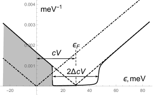
Figure 3: Linear low energy DOS of pure graphene (dash-dotted line), and its restructured DOS (solid line) under LM impurities with on-site disorder strength $V=W/2$ and concentration $c=10^{-2}$ that presents: 1) the global energy shift by $cV$ and 2) the spectrum gap of $2\Delta c|V|$ around the shifted Fermi level (dashed line), due to the asymmetry of impurity occupation of host sublattices, $\Delta c=6\cdot 10^{-3}$. The range of filled quasiparticle states is shadowed.

In the most natural case of equal sublattice occupancies, $\Delta c=0$, the inter-band scattering (the $\hat{\sigma}_{1}$-term) cancels out and Eq. 33 takes particularly simple form. The overall impurity effect gets reduced just to a simple mean-field shift of the energy reference by $cV$ with no other notable changes in the observable properties. However, if there exists a certain occupational asymmetry between the two sublattices, $\Delta c\neq 0$, for instance due to lattice buckling, the spectral Eq. 32 would retain also a finite off-diagonal term. As a consequence, apart of the Fermi level shift $cV$, there appears also a splitting of the valence and conduction bands quantified by a finite gap value $2\Delta c|V|$, see Eq. 33. This would, respectively, modify the low energy DOS, and the corresponding gapped-like analog of Eq. 20 reads:

$$\rho(\varepsilon)\approx\frac{2|\varepsilon-cV|}{W^{2}}\,\Theta\left[(\varepsilon-cV)^{2}-(\Delta cV)^{2}\right]\,,$$ (34)

recovering purely linear behavior beyond the gap, unlike peculiar behaviors near impurity resonances in AM (see in detail in the next sections). Validity of this simplest Born approximation picture is also confirmed by the full T-matrix calculation for DOS at the choice of $V=W/2$, $c=10^{-2}$ and $\Delta c=6\cdot 10^{-3}$, displayed in Fig. 3.

IV Anderson’s impurity model, a general discussion

Anderson model (AM) differs from the Lifshitz one by considering impurities beyond the host sites, for instance, impurity adatoms over the graphene plane. The model introduces new degrees of freedom into the system by means of impurity Fermi operators $c_{\bf r}$. We label them by in-plane projection vectors ${\bf r}$ that are not necessarily lattice sites, and hence not bearing the sublattice index. Another specifics of AM is the dynamics of impurity perturbation, which is described by two independent parameters; the impurity energy level (on-site energy) $\varepsilon_{0}$, and the hopping (coupling) parameter $\omega$ of its hybridization with carbons at nearest neighbor graphene sites ${\bf n}_{j}$. In terms of local operators, this perturbation Hamiltonian reads:

$$H_{\rm AM}=\sum_{\bf r}\left[\varepsilon_{0}c_{\bf r}^{\dagger}c_{\bf r}^{\phantom{\dagger}}+\omega\sum_{\langle{\bf r},{\bf n}_{j}\rangle}\left(b_{{\bf n}_{j}}^{\dagger}c_{\bf r}^{\phantom{\dagger}}+h.c.\right)\right].$$ (35)

Also a GF treatment of this perturbation was proposed previously Skrypnyk and Loktev (2013) and here we shall develop it in a more general context. Thus, expressing again the local atomic operators $b_{{\bf n}_{j}}^{\dagger}$ through the graphene band $\psi^{\dagger}_{\bf k}$ spinors, Eq. 13, the above Hamiltonian is brought to the form:

$$H_{\rm AM} = \sum_{{\bf r}}\left[\varepsilon_{0}c_{{\bf r}}^{\dagger}c_{{\bf r}}^{\phantom{\dagger}}\right.$$ (36)

$$+ \left.\frac{\omega}{\sqrt{N}}\sum_{\bf k}\left(\psi_{\bf k}^{\dagger}\,u_{{\bf k},{\bf r}}^{\phantom{\dagger}}\,c_{{\bf r}}^{\phantom{\dagger}}+h.c.\right)\right],$$

where the form-factor (column) spinor $u_{{\bf k},{\bf r}}$ reflects the local symmetry of an impurity at position ${\bf r}$ and is given as:

$$u_{{\bf k},{\bf r}}=\frac{1}{\sqrt{2}}\sum_{\langle{\bf r},{\bf n}_{j}\rangle}{\rm e}^{i\phi_{{\bf n}_{j},{\bf k}}}\left(\begin{array}[]{c}1\\ (-1)^{j-1}\end{array}\right),$$ (37)

with the hopping phases $\phi_{{\bf n}_{j},{\bf k}}$ by Eq. 5.

Considering the equation of motion for the momentum-diagonal GF matrix we have:

$$\hat{G}_{\bf k}=\hat{G}_{\bf k}^{(0)}+\frac{\omega}{\sqrt{N}}\sum_{{\bf r}}\hat{G}_{\bf k}^{(0)}\,u_{{\bf k},{\bf r}}^{\phantom{\dagger}}\,\langle\langle c_{\bf r}^{\phantom{\dagger}}|\psi_{\bf k}^{\dagger}\rangle\rangle,$$ (38)

where the impurity-host GF (forming a row spinor in band indices), $\langle\langle c_{\bf r}^{\phantom{\dagger}}|\psi_{\bf k}^{\dagger}\rangle\rangle$, can be excluded from that equation using its own equation of motion:

$$\langle\langle c_{\bf r}^{\phantom{\dagger}}|\psi_{\bf k}^{\dagger}\rangle\rangle=\frac{\omega}{\left(\varepsilon-\varepsilon_{0}\right)\sqrt{N}}\sum_{{\bf k}^{\prime}}u_{{\bf r},{\bf k}^{\prime}}^{\dagger}\,\hat{G}_{{\bf k}^{\prime},{\bf k}}^{\phantom{\dagger}},.$$ (39)

This effectively decouples host-host and impurity-host GF’s to give:

$$\hat{G}_{\bf k}=\hat{G}_{\bf k}^{(0)}+\frac{1}{N}\sum_{{\bf r},{\bf k}^{\prime}}\hat{G}_{\bf k}^{(0)}\,\hat{V}_{{\bf r},{\bf k},{\bf k}^{\prime}}^{\phantom{\dagger}}\,\hat{G}_{{\bf k}^{\prime},{\bf k}}\,,$$ (40)

where the effective $2\times 2$ scattering matrix (in the band indices) for the impurity at ${\bf r}$ position reads:

$$\hat{V}_{{\bf r},{\bf k},{\bf k}^{\prime}}^{\phantom{\dagger}}=u_{{\bf k},{\bf r}}^{\phantom{\dagger}}\,\frac{\omega^{2}}{\varepsilon-\varepsilon_{0}}\,u_{{\bf k}^{\prime},{\bf r}}^{\dagger}\,.$$ (41)

The detailed structure of the $\hat{V}_{{\bf r},{\bf k},{\bf k}^{\prime}}$ matrices follows from the particular $j$-types of graphene sites ${\bf n}_{j}$, neighbors to ${\bf r}$, as in Eq. 37.

Despite the AM scattering matrix, Eq. 41, differs from the former LM one, Eq. 23, by its explicit energy dependence, it generates formally the same GE series in powers of $c$ as the LM result. For a general scattering problem, the momentum diagonal T-matrix with the corresponding $u_{{\bf k},{\bf r}}$ spinor reads:

$$\hat{T}_{{\bf r},{\bf k}}(\varepsilon)=\frac{\omega^{2}u_{{\bf k},{\bf r}}^{\phantom{\dagger}}\,u_{{\bf k},{\bf r}}^{{\dagger}}}{\varepsilon-\varepsilon_{0}-\omega^{2}N^{-1}\,\sum_{{\bf k}^{\prime}}u_{{\bf k}^{\prime},{\bf r}}^{{\dagger}}\,\hat{G}_{{\bf k}^{\prime}}^{(0)}(\varepsilon)\,u_{{\bf k}^{\prime},{\bf r}}^{\phantom{\dagger}}},$$ (42)

formally the same as for the LM scenario, consult Eqs. 28 and 29.

Figure 4: Different positions of AM impurities (yellow circles) over a graphene layer: i) t-positions, atop of carbon lattice sites of 1- or 2- types, ii) b-positions, over centers of bridges between 1- and 2-type lattice sites (one of three possible bridges shown), iii) h-position, over the center of a hexagonal cell.

The most natural positions discussed in what follows are those shown in Fig. 4 and categorized as:

i) top position (t-position), impurity projects just on a host lattice site ${\bf n}_{j}$ and such position can be indexed by this $j$,

ii) bridge position (b-position), impurity projects on a midpoint ${\bf r}$ between two carbons belonging to the opposite sublattices. In this case the positions of two hybridizing carbons are: ${\bf n}_{1,i}={\bf r}-\boldsymbol{\delta}_{i}/2$, and ${\bf n}_{2,i}={\bf r}+\boldsymbol{\delta}_{i}/2$, where three nearest-neighbor vectors $\boldsymbol{\delta}_{i=1,2,3}$ are displayed in Fig. 1. The corresponding bridge configurations b${}_{\boldsymbol{\delta}_{i}}$ are related through $\pm 120^{\circ}$ rotations.

iii) hollow position (h-position), impurity projects on a center of hexagonal lattice cell, in this case we have three nearest neighbor sites ${\bf n}_{1,i}={\bf r}+\boldsymbol{\delta}_{i}$, $i=1,2,3$ from the sublattice 1, and three such sites ${\bf n}_{2,i}={\bf r}-\boldsymbol{\delta}_{i}$ from the sublattice 2.

So, generally, there are two possible types of t-position (t_j), three types of b-position (b_δ), and a single type of h-position. Obviously, two t_j-types can be occupied either symmetrically or asymmetrically in $j$, while such occupations of three b_δ-types and of single h-type are $j$-independent. A special difference between them is yet in possible momentum dependence for the self-energy and T-matrix (besides their common $\varepsilon$ dependence). This effect is especially pronounced in the h-case, making it qualitatively different from the t- and b-cases. It can be also shown that, due to their different couplings to the graphene host, the listed three positions will contribute into the system dynamics in different energy ranges, and therefore they can be considered independently.

Table 1: AM tight-binding parameters $\varepsilon_{0},\omega$ for some representative top impurity adatoms on graphene, including the “gauge” value $\omega^{\ast}$ discriminating between weak, strong and intermediate perturbations.

Atom	Cu	Cu	H	F
Position	t-	b-	t-	t-
$\varepsilon_{0}$ (eV)	0.08	0.02	0.16	-2.2
$\omega$ (eV)	0.81	0.54	7.5	5.5
$\omega^{\ast}$ (eV)	1.99	1.73	2.17	4.35

Available data suggest that adsorption in the top position seems to be favorable for light atoms like hydrogen  Boukhvalov et al. (2008); Gmitra et al. (2013), fluorine Wu et al. (2008); Şahin et al. (2011); Irmer et al. (2015) and copper  Wu et al. (2009); Amft et al. (2011); Frank et al. (2017), the heavier gold atom Chan et al. (2008); Amft et al. (2011), and, for example, also the light ad-molecule methyl Zollner et al. (2016). A special case is the vacancy which as was mentioned induces a zero-energy mode Ducastelle (2013); Pereira et al. (2006); Peres et al. (2006); Pereira et al. (2008).

In the following sections we consider in more detail each of the above mentioned impurity positions, and analyze reconstructed spectra and localization properties of the corresponding eigenstates. This will be illustrated for several particular examples of impurity adatoms whose known AM parameters are collected in Table 1.

V Anderson’s impurities at top position

For a t-position impurity located at ${\bf r}_{j}$, the form-factor spinor, Eq. 37, is realized as:

$$u_{{\bf r}_{j},{\bf k}}=\frac{1}{\sqrt{2}}{\rm e}^{i\phi_{{\bf r}_{j},{\bf k}}}\left(\begin{array}[]{c}1\\ (-1)^{j-1}\end{array}\right),$$ (43)

and the corresponding effective scattering matrix then reads:

$$\hat{V}_{{\bf r}_{j},{\bf k},{\bf k}^{\prime}}=\frac{\omega^{2}}{\varepsilon-\varepsilon_{0}}\exp\left[i(\phi_{{\bf r}_{j},{\bf k}}-\phi_{{\bf r}_{j},{\bf k}^{\prime}})\right]\hat{m}_{j}$$ (44)

with the same $\hat{m}_{j}$ matrices as in the LM case, see Eq. 24. Defining the energy dependent effective scattering potential:

$$V(\varepsilon)=\frac{\omega^{2}}{\varepsilon-\varepsilon_{0}},$$

the corresponding T-matrix in AM takes an analogous form to the LM case, Eq. 29: $\hat{T}_{{\bf r}_{j},{\bf k}}=T_{t}(\varepsilon)\hat{m}_{j}$, where the scalar T-factor:

$$T_{t}(\varepsilon)=\frac{V(\varepsilon)}{1-V(\varepsilon)G^{(0)}(\varepsilon)}=\frac{\omega^{2}}{\varepsilon-\varepsilon_{0}-\omega^{2}G^{(0)}(\varepsilon)}\,,$$ (45)

is, alike the LM case, momentum and sublattice independent.

The condition for impurity resonances, the real part of T-matrix denominator becoming zero, leads here to the explicit equation:

$$\varepsilon_{res}\left(1+\frac{\omega^{2}}{W^{2}}\ln\frac{W^{2}-\varepsilon_{res}^{2}}{\varepsilon_{res}^{2}}\right)=\varepsilon_{0}.$$ (46)

Comparing to the LM case, Eq. 30, there are no special restrictions on AM perturbation parameters for such resonance to appear. It is a matter of fact that the hybridization $\omega$ between the adatom and graphene host is responsible for the shifts of the resonance energy, $\varepsilon_{res}$, towards zero, when comparing with the initial atomic level $\varepsilon_{0}$ (supposing the latter satisfies $\varepsilon_{0}^{2}<W^{2}/2$). The relative magnitude of this shift depends on the coupling parameter $\omega$ compared to its “gauge” value:

$$\omega^{\ast}=W/\sqrt{\ln\left(W^{2}/\varepsilon_{0}^{2}-1\right)}.$$ (47)

This distinguishes between the three coupling types:

(a) weak, $|\varepsilon_{res}-\varepsilon_{0}|\ll|\varepsilon_{0}|$, for $|\omega|\ll\omega^{\ast}$,

(b) strong, $|\varepsilon_{res}|\ll|\varepsilon_{0}|$, for $|\omega|\gg\omega^{\ast}$, and

(c) intermediate, $|\varepsilon_{res}-\varepsilon_{0}|\sim|\varepsilon_{0}|$, for $|\omega|\sim\omega^{\ast}$.

Then, from the comparison of $\omega$ to $\omega^{\ast}$ for the cases in Table 1, Cu adatoms at t- and b-positions can be classified as weakly coupled, H adatoms at t-position as strongly coupled, and F adatoms at t-position as intermediate coupled.

In particular, for weakly coupled impurities, the approximate solution of Eq. 46 is given within to logarithmic accuracy as:

$$\varepsilon_{res}\approx\frac{\varepsilon_{0}}{1+(\omega/\omega^{\ast})^{2}}.$$ (48)

Our next studies consider the band structure reconstruction for symmetric and asymmetric sublattice occupancies, and the arise of mobility edges for t-positioned AM impurities. The starting point for those discussions is the spectral equation for the inverse of momentum-diagonal GF matrix, $\hat{G}_{\bf k}^{-1}(\varepsilon)$. In analogy with the LM, Eq. 32, the T-matrix approximation averaged in disorder by t-position AM impurities reads here:

$$\hat{G}_{\bf k}^{-1}(\varepsilon)=\bigl{[}\varepsilon-cT_{t}(\varepsilon)\bigr{]}\hat{1}-\varepsilon_{q}\hat{\sigma}_{3}-\Delta cT_{t}(\varepsilon)\hat{\sigma}_{1}\,.$$ (49)

The restructured band spectrum in presence of impurities is usually sought as the roots of secular equation Bonch-Bruevich and Tyablikov (2015):

$${\rm Det}\,\hat{G}_{\bf k}^{-1}(\varepsilon)=0.$$ (50)

In fact, this is an essential reduction of the underlying eigenvalue problem for the full, translationally non-invariant Hamiltonian $H_{0}+H_{\rm AM}$ with randomly disordered impurities Lifshitz et al. (1988) that intrinsically admit alternation of the band-like and localized ranges, the celebrated metal-insulator transitions Mott (1967). The above secular Eq. 50 with use of Eq. 49 provides just a disorder averaged approximation where the quasi-momentum ${\bf k}$ is no more an exact quantum number as it was for the unperturbed band spectrum, e.g. in Eq. 2.

One way how to construct solutions of the secular Eq. 50 is to look at energy vs quasi-momentum relation, we call it energy-projected solution (EPS). Here, for a given real ${\bf k}$, hybridization of each initial $\pm\varepsilon_{q}$ subband with the impurity resonance level $\varepsilon_{res}$ generates up to four complex energy roots of Eq. 50: $\varepsilon=E_{j,{\bf k}}+i\Gamma_{j,{\bf k}}$, $j=1,\dots,4$. Their real parts $E_{j,{\bf k}}$ approximate the restructured dispersion laws (for the band-like energy ranges, see also discussion later), while the imaginary parts do the lifetimes $\tau_{j,{\bf k}}\sim\hbar/\Gamma_{j,{\bf k}}$ of such quasiparticles. However, a complicated functional form of $T_{t}(\varepsilon)$, Eq. 45, especially of the locator GF in its denominator, makes analytical finding of EPS a formidable task. Therefore, some simplifications are often employed. For example, one identifies restructured energies $E_{j,{\bf k}}$ just with the solutions of the real part of Eq. 50:

$${\rm Re}\bigl{[}{\rm Det}\,\hat{G}_{\bf k}^{-1}(\varepsilon)\bigr{]}=0\,,$$ (51)

or, goes even simpler, and moves the real part operation deeper into the expression. Particularly, from the determinant to the self-energy matrix:

$${\rm Re}\bigl{[}{\rm Det}\,\hat{G}_{\bf k}^{-1}\bigr{]}\to{\rm Det}\bigl{[}(\hat{G}_{\bf k}^{(0)})^{-1}-{\rm Re}\,\hat{\Sigma}_{\bf k}\bigr{]}$$ (52)

or even further just to its denominator:

$${\rm Re}\,\hat{\Sigma}_{\bf k}\to\frac{\omega^{2}\sum_{j}c_{j}\hat{m}_{j}}{\varepsilon-\varepsilon_{0}-\omega^{2}{\rm Re}\,G^{(0)}(\varepsilon)}.$$ (53)

Then, linearizing ${\rm Re}\,G^{(0)}(\varepsilon)$ in $\varepsilon$ around the resonance allows to find the restructured energies $E_{j,{\bf k}}$ as functions of quasi-momenta ${\bf k}$ in a relatively simple and closed form.

However, there is an alternative way to search for the band-like solutions of Eq. 50 in so-called inverted form, i.e. looking for functional dependence of quasimomenta in terms of energy: ${\bf k}(\varepsilon)$. Such (in principle complex) solution we call the momentum-projected solution (MPS). In the present case, even keeping the full T-matrix form, the resulting equation turns to be just an algebraic equation (at most of cubic order) for ${\bf k}(\varepsilon)$ or, more precisely, for $q(\varepsilon,\theta)$, where $\theta$ stands for the azimuthal angle of the quasimomentum ${\bf q}={\bf k}-{\bf K}^{(\prime)}$ (measured relative to the Dirac point). In the isotropic case, Eqs. 6, 9, one gets the radial component $q$ as a function of $\varepsilon$ only. It is obvious that presence of T-matrix imaginary part (relevant for damping effects) makes this $q(\varepsilon)$ generally complex-valued.

Thus, for t-impurities we obtain the MPS explicitly as:

$$q(\varepsilon)=\frac{q_{max}}{W}\sqrt{\left[\varepsilon-cT_{t}(\varepsilon)\right]^{2}-\left[\Delta cT_{t}(\varepsilon)\right]^{2}}\,,$$ (54)

with the full complex form of $T_{t}(\varepsilon)$ given by Eq. 45. Another notable advantage of this solution is in providing a single-valued $q(\varepsilon)$ function, instead of four EPS functions.

Both indicated types of spectral solutions, EPS and MPS, are employed in the following analysis of different AM impurity cases.

V.1 Weakly coupled AM t-impurities with symmetric occupancy

Beginning from the symmetric case, $c_{1}=c_{2}=c/2$ and $\Delta c=0$, one has the inverse GF matrix, Eq. 49, purely diagonal in the sublattice indices, and so the secular equation, Eq. 51, factorizes:

$$\mathrm{Re}\left[\left(\varepsilon-\varepsilon_{q}-cT_{t}(\varepsilon)\right)\left(\varepsilon+\varepsilon_{\bf k}-cT_{t}(\varepsilon)\right)\right]=0\,.$$ (55)

The above suggested linearization of $T_{t}(\varepsilon)$ denominator, brings this function to the form:

$$T_{t}(\varepsilon)\approx\frac{\tilde{\omega}^{2}}{\varepsilon-\varepsilon_{res}-i\Gamma(\varepsilon)},$$ (56)

where the renormalized hybridization strength $\tilde{\omega}$ and the damping term $\Gamma(\varepsilon)$ read:

$$\tilde{\omega}^{2}=\omega^{2}\varepsilon_{res}/\varepsilon_{0},\ \ \ \ \Gamma(\varepsilon)=\pi|\varepsilon|(\tilde{\omega}/W)^{2}\,.$$ (57)

For weakly coupled AM t-impurities, such linearization is well justified over the whole low-energy range (except for extremely low values, $|\varepsilon|\lesssim W{\rm e}^{-(W/2\tilde{\omega})^{2}}$, the latter being as small as $\approx 0.5\mu$eV for the Cu t-case).

Then, in neglect of damping in Eq. 56, justified for energies not too close to the resonance, $|\varepsilon-\varepsilon_{res}|\gg\Gamma(\varepsilon_{res})$, the factors in Eq. 55 provide two decoupled quadratic equations for $\varepsilon$. The resulting EPS’s define the explicit low-energy dispersion laws:

$$E_{{}^{1}_{3},{\bf k}} = E_{{}^{1}_{3},{\bf q}+{\bf K}^{(\prime)}}\equiv E_{{}^{1}_{3},q}$$ (58)

$$= \frac{\varepsilon_{res}+\varepsilon_{q}\pm\sqrt{\left(\varepsilon_{res}-\varepsilon_{q}\right)^{2}+4c{\tilde{\omega}}^{2}}}{2}\,,$$

$$E_{{}^{2}_{4},{\bf k}} = E_{{}^{2}_{4},{\bf q}+{\bf K}^{(\prime)}}\equiv E_{{}^{2}_{4},q}$$ (59)

$$= \frac{\varepsilon_{res}-\varepsilon_{q}\pm\sqrt{\left(\varepsilon_{res}+\varepsilon_{q}\right)^{2}+4c{\tilde{\omega}}^{2}}}{2}\,.$$

In the above formulas the subscripts 1, 2 apply to the plus sign, and 3, 4 do to the minus sign. Their validity is restricted to momenta close to the valleys centers, therefore $\varepsilon_{q}$ can be taken in the linearized form of Eq. 6.

The restructured energy spectrum around the ${\bf K}$ point for the case of Cu adatoms residing equally on graphene sublattices with concentration $c=0.035$ is displayed in Fig. 5. It illustrates the above mentioned hybridization of two initial graphene subbands $\pm\varepsilon_{q}$ with the resonance level $\varepsilon_{res}$ to produce the energy subbands $E_{j,q}$. Those do not overlap and fill almost completely the initial spectrum range $(-W,W)$. With growing $c$, the restructured energy spectrum displays a conjunction of two known scenarios that can take place when a single-band interacts with the impurity level:

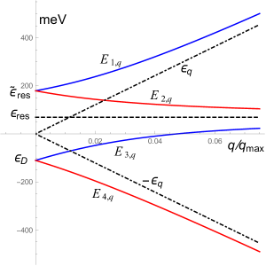
Figure 5: Restructured band spectrum (in neglect of its damping) vs reduced quasi-momentum for graphene with Cu t-impurities at concentration $c=3.5\cdot 10^{-2}$ and symmetric sublattice occupation, Eqs. 58, 59 (blue and red lines), compared to that for pure graphene, $\pm\varepsilon_{q}$ (dash-dotted lines). The quasi-gap between the resonance level $\varepsilon_{res}\approx 69$ meV (dashed line) and the bottom of $E_{1,q}$ subband, $\tilde{\varepsilon}_{res}\approx 180$ meV, gets filled by the impurity subband $E_{2,q}$ states (see text).

a) Formation of a narrow quasi-gap Ivanov and Pogorelov (1979) near the resonance level $\varepsilon_{res}$ which separates the branches $E_{1,q}$ and $E_{3,q}$. The quasi-gap exhausts the energy window (assuming $\varepsilon_{0}>0$) between ${\rm max}\,E_{3,q}\approx\varepsilon_{res}$ and ${\rm min}\,E_{1,q}$, given by:

$$\tilde{\varepsilon}_{res}=\varepsilon_{res}\frac{1+\sqrt{1+c/c^{\ast}}}{2},$$ (60)

with $c^{\ast}=\varepsilon_{0}\varepsilon_{res}/4\omega^{2}$ (for Cu t-case, $c^{\ast}\approx 2\cdot 10^{-3}$). Until $c\ll c^{\ast}$, the quasi-gap width grows linearly: $\approx\,\varepsilon_{res}c/4c^{\ast}$, then slowing down to $\approx\,\varepsilon_{res}(\sqrt{c/c^{\ast}}-1)/2$ at $c\gg c^{\ast}$. Generally, this results from a strong enough mixing between the intersecting $\varepsilon_{q}$ band and $\varepsilon_{res}$ level (anti-crossing).

b) Formation of a narrow impurity subband Ivanov et al. (1987) near the localized level, the $E_{2,q}$ branch that fills the above indicated quasi-gap, and of a detached weakly affected valence band $E_{4,q}$. The explanation of that is also very intuitive; the impurity level lies far from the graphene valence band $-\varepsilon_{q}<0$, and, due to the weakness of their interaction, both just slightly modify their dispersions ($E_{2,q}$ staying almost dispersionless and $E_{4,q}$ almost aligned with the original $-\varepsilon_{q}$).

Noteworthy, in the symmetric case ($\Delta c=0$), the a-type quasi-gap gets completely filled with the states from the b-type impurity subband, though this filling turns incomplete for an asymmetric occupancy ($\Delta c\neq 0$).

Technically, when considering the full complex T-matrix (either linearized or exact), analytic derivation of EPS from Eq. 55 may turn complicated. On the other hand, the MPS, see Eq. 54, is quite simple and does not require linearization of $T_{t}(\varepsilon)$ or neglect of its damping.

Within the T-matrix approximation, the momentum-diagonal GF can be written in terms of the unperturbed GF, Eq. 17, but with the shifted argument:

$$\hat{G}_{\bf k}(\varepsilon)=\hat{G}_{\bf k}^{(0)}\bigl{(}\varepsilon-cT_{t}(\varepsilon)\bigr{)}\,.$$ (61)

This facilitates DOS per unit cell in presence of AM impurities, taking also into account their additional degrees of freedom (by the $c_{\bf r}$ operators) so that the total DOS gets composed of two parts:

$$\rho(\varepsilon)=\rho_{host}(\varepsilon)+\rho_{imp}(\varepsilon),$$ (62)

in an extension of the simpler LM case.

The host part, $\rho_{host}(\varepsilon)=(\pi N)^{-1}\sum_{\bf k}{\rm Im\,Tr}\,\hat{G}_{\bf k}$, is analogous to Eqs. 20, 34, but with the variable energy shift:

$$\rho_{host}(\varepsilon)=\frac{2}{\pi}{\rm Im}\,G^{(0)}\bigl{(}\varepsilon-cT_{t}(\varepsilon)\bigr{)},$$ (63)

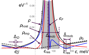
Figure 6: Restructured DOS of graphene under Cu impurities as in Fig. 5, the total value $\rho$ (black line) and its host, $\rho_{host}$ (blue line), and impurity, $\rho_{imp}$ (red line), components, referred to the pure graphene linear DOS, $\rho_{0}$ (dashed line). The mobility gaps $\Delta_{mob}$, $\tilde{\Delta}_{mob}$, and $\Delta_{\rm D}$ (see below) are shadowed.

As shown in Fig. 6, this DOS part displays a sharp peak at $\varepsilon_{res}$, and sharp drops towards zero at the quasi-gap edge, $\tilde{\varepsilon}_{res}=\min{E_{1,{\bf k}}}$, and at $\varepsilon_{D}=\max{E_{4,{\bf k}}}\approx-c\omega^{2}/\varepsilon_{0}$, in consistency with the spectrum dispersion in Fig. 5. The last two energies can be seen as “split Dirac points”: while the  $\min$ of conduction band and the $\max$ of valence band in pure graphene join at the Dirac points, the corresponding $\min$ and $\max$ of reconstructed bands in the AM case run off (see also the discussion below).

The impurity DOS part, counting the adatom degrees of freedom, reads:

$$\rho_{imp}(\varepsilon)=\frac{1}{\pi}{\rm Im}\,\frac{1}{N}\sum_{\bf r}\langle\langle c_{\bf r}^{\phantom{\dagger}}|c_{\bf r}^{\dagger}\rangle\rangle\approx\frac{c}{\pi\omega^{2}}\,{\rm Im}\,T_{t}(\varepsilon),$$ (64)

and, with use of the approximated T-matrix, Eq. 56, it takes the conventional Lorentzian form:

$$\rho_{imp}(\varepsilon)\approx\frac{c\varepsilon_{res}}{\pi\varepsilon_{0}}\frac{\Gamma(\varepsilon)}{\left(\varepsilon-\varepsilon_{res}\right)^{2}+\Gamma^{2}(\varepsilon)}.$$ (65)

Comparison of the related contributions to the total $\rho(\varepsilon)$ in Fig. 6 shows that $\rho_{imp}(\varepsilon)$ (red line) generally dominates inside the localization ranges $\Delta_{mob}$, $\tilde{\Delta}_{mob}$, and $\Delta_{\rm D}$ (see discussion below) while $\rho_{host}(\varepsilon)$ dominates outside these ranges.

As already mentioned, the specifics of this band restructuring is the shift of DOS: the zero (Dirac) point moves to $\varepsilon_{D}=E_{3,0}=E_{4,0}\approx-c\omega^{2}/\varepsilon_{0}$. A fully analogous effect was already met within LM, see the mean-field shift by $cV$ in Fig. 3. As a word of caution, the value of $\varepsilon_{D}\approx-c\omega^{2}/\varepsilon_{0}$ lies beyond validity of the linearized Eq. 56, and was obtained from the exact T-matrix expression, Eq. 45, however, for weakly coupled impurities, it only slightly differs from $-c\omega^{2}/\varepsilon_{res}$ resulting from Eq. 56. This plausibly justifies the dispersion formulae, Eqs. 58, 59, for such impurities over the whole low-energy range.

V.2 Ioffe-Regel-Mott criterium, and mobility gaps

The presented formal picture of the disorder averaged restructured spectrum at finite concentration of AM impurities can be considered as consistent and reliable only if the lifetime $\tau(E_{\bf k})$ of the band-like states with quasi-momentum ${\bf k}$ and energy $E_{\bf k}$ is substantially longer then the intrinsic oscillation period $\lambda_{\bf k}/v_{\bf k}$ of the associated Bloch-like wave ($\lambda_{\bf k}$ being its wavelength and $v_{\bf k}$ the group velocity), i.e.

$$\frac{\lambda_{\bf k}}{v_{\bf k}}\ll\tau(E_{\bf k}).$$ (66)

This qualitative and phenomenological statement is known as the Ioffe-Regel-Mott (IRM) criterion Ioffe and Regel (1960); Mott (1967). In the simplest case of one parabolic band centered at the $\Gamma$-point of BZ, the IRM criterion for an extended state with quasi-momentum ${\bf k}$ and energy $E_{\bf k}$ is commonly written as:

$$\left.{\bf k}\cdot{\mathbf{\nabla}}_{\bf k}\,E_{\bf k}\right|_{E_{\bf k}}\gg\hbar\,\tau^{-1}(E_{\bf k}),$$ (67)

where one identifies $\lambda_{\bf k}=1/|{\bf k}|$ and ${\bf v}_{{\bf k}}=\hbar^{-1}{\mathbf{\nabla}}_{\bf k}E_{\bf k}$. If, for given $E_{\bf k}$, the lifetime $\tau(E_{\bf k})$ is too short so that IRM criterion breaks down, and the related state is no more considered as wave-like (or extended), but localized. Moreover, accordingly to Mott Mott (1967), if this criterion fails at least for one ${\bf k}$ on the isoenergetic $E_{\bf k}=\varepsilon$ surface (line), then all the states at this energy $\varepsilon$ become localized at impurity centers (or impurity clusters). Such onset of localization emerges within a certain continuous energy range called the Mott mobility gap Mott (1967), and a threshold between the extended and localized ranges is called the mobility edge. One can try to estimate this edge position by passing from $\gg$ to $\sim$ in Eq. 67, and by using dispersion laws, Eqs. 58, 59, but taking into account that the used common definition of group velocity and wave length become imprecise near Dirac point, leaving an uncertainty margin for such procedure. The case of graphene is described below.

At low enough impurity concentrations, the inverse lifetime is well approximated just by the imaginary part of T-matrix, $\hbar\tau^{-1}(\varepsilon)=c\,{\rm Im}\,T_{t}(\varepsilon)$, and the latter is given in the vicinity of $\varepsilon_{res}$, for example, by the linearized Eq. 56. That can be used as the right hand side in the IRM criterion for a given ${\bf k}$-state. The low energy states of graphene have quasi-momenta ${\bf k}$ located near the K-points instead of the $\Gamma$-point and the corresponding Bloch waves are superpositions of a standing ${\bf K}$-wave and running ${\bf q}$-waves, but only the latter define the relevant wavelength scale for the IRM-criterion. Then the product ${\bf k}\cdot{\mathbf{\nabla}}_{\bf k}$ gets naturally substituted by ${\bf q}\cdot{\mathbf{\nabla}}_{\bf q}=q\tfrac{\partial}{\partial q}$, so that Eq. 67 reduces to:

$$\left|{q\frac{\partial E_{\bf q}}{\partial q}\Bigr{|}_{E_{\bf q}}}\right|\gg c\,{\rm Im}\,T_{t}(E_{\bf q})=\hbar\,\tau^{-1}(E_{\bf q}).$$ (68)

This is only half of the story, while taking the momentum derivatives of the EPS dispersion $E_{\bf q}$, Eqs. 58, 59, is quite impractical. However, employing MPS, $q(\varepsilon,\theta)$, and the reciprocal derivative, $\partial\varepsilon/\partial q=\left(\partial q/\partial\varepsilon\right)^{-1}$, allow to circumvent that technical problem and formulate IRM in the equivalent but alternative way:

$$\left|\frac{{\rm Re\,}q(\varepsilon,\theta)}{\partial{\rm Re\,}q(\varepsilon,\theta)/\partial\varepsilon}\right|\gg\hbar\,\tau^{-1}(\varepsilon).$$ (69)

Here the relevant wave-number of a Bloch-like wave along angle $\theta$ is represented by ${\rm Re\,}q(\varepsilon,\theta)$, the real part of respective MPS, which can admit anisotropy and that does not require linearized T-matrix. For the considered isotropic t-case, this corresponds to the real part of Eq. 54, that can be used in Eq. 69. Some more general MPS and the corresponding mobility edge analyzes will be encountered later.

Let us estimate ranges for IRM to fail, for that we consider the limiting form of Eq. 69:

$$\left|\frac{{\rm Re\,}q(\varepsilon)}{\partial{\rm Re\,}q(\varepsilon)/\partial\varepsilon}\right|\gtrsim\hbar\tau^{-1}(\varepsilon)$$ (70)

Reaching this limit can be either due to decreasing l.h.s. of Eq. 69 or due to growing its r.h.s, and therefore those two cases have different physical origins. The first case can take place near the split Dirac points, $\tilde{\varepsilon}_{res}$ and $\varepsilon_{\rm D}$, where the relevant momenta tends to go to zero, $q\to 0$, there the analysis can be simplified by using a linearized in $q$ MPS (LMPS). The second possibility occurs near $\varepsilon_{res}$ where the relevant momenta correspond to $\varepsilon_{q}\simeq\varepsilon_{res}$ (see Fig. 5).

Let us estimate for the second case the critical concentration $c_{0}$, where the IRM breaks down. With growing impurity concentration $c$, the failure of IRM is firstly expected directly at energy $\varepsilon_{res}$, where the inverse lifetime reaches its maximum:

$$\hbar\,\tau^{-1}(\varepsilon_{res})=c\,{\rm Im}\,T_{t}(\varepsilon_{res})=\frac{cW^{2}}{\pi|\varepsilon_{res}|}.$$ (71)

Contrary, using the simplest LMPS, namely, the unperturbed MPS just for the plain graphene: $q(\varepsilon)\approx q_{max}|\varepsilon|/W$, the l.h.s. of Eq. 70 reduces just to $|\varepsilon|$. Then, comparing $|\varepsilon|$ at resonance energy $\varepsilon_{res}$ with $\hbar\,\tau^{-1}(\varepsilon_{res})$, we find that IRM inequality holds at $\varepsilon=\varepsilon_{res}$ until the impurity concentration stays below the critical value:

$$c\lesssim c_{0}=\pi\left(\frac{\varepsilon_{res}}{W}\right)^{2}.$$ (72)

This just corresponds to the condition that the average distance between neighboring impurities ${\bar{r}}\sim ac^{-1/2}$ exceeds the resonance state radius $r_{res}\sim aW/\varepsilon_{res}$, protecting the coherence of quasi-particles with energies near $\varepsilon_{res}$ (including those near $\tilde{\varepsilon}_{res}$) against random impurity scatterings.

Above this critical concentration, $c>c_{0}$, the IRM condition breaks down around $\varepsilon_{res}$ within a certain finite energy width $\Delta_{mob}$, the Mott mobility gap, which gets filled with the localized levels. Using the same unperturbed LMPS for l.h.s. of Eq. 70 and the Lorentzian form of $\hbar\,\tau^{-1}(\varepsilon)$ near $\varepsilon_{res}$, similar to Eq. 65, leads to the estimate:

$$\Delta_{mob}\sim\frac{\tilde{\omega}^{2}}{W}\sqrt{c-c_{0}},$$ (73)

though only valid until $c-c_{0}\lesssim c_{0}$. However, even at $c\gg c_{0}$ this development can be still traced analytically. For instance, the result of Eq. 73 stays valid for the lower edge of $\Delta_{mob}$, only formed by the states near $\varepsilon_{res}$. But for its upper edge, the inverse lifetime $\hbar\,\tau^{-1}(\varepsilon)$ gets also a growing contribution from the vicinity of impurity band edge $\tilde{\varepsilon}_{res}$ and the corresponding term, $\tilde{\Delta}_{mob}$, can be estimated with the proper LMPS, $q(\varepsilon)\approx q_{max}|\varepsilon-\tilde{\varepsilon}_{res}|/W$, used in Eq. 70:

$$\tilde{\Delta}_{mob}\sim\hbar\tau^{-1}(\tilde{\varepsilon}_{res}-\tilde{\Delta}_{mob})\sim\frac{c^{1/3}\tilde{\omega}^{4/3}\varepsilon_{res}^{1/3}}{W^{2/3}}.$$ (74)

The latter value exceeds the impurity band width, $c\tilde{\omega}^{2}/\varepsilon_{res}$, formally defined by Eq. 59, making this band unphysical as far as $c\lesssim\sqrt{c_{0}c_{\ast}}$, where $c_{\ast}=(\varepsilon_{res}/\tilde{\omega})^{2}$.

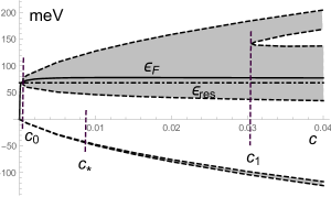
Figure 7: Variation of mobility gaps (shadowed areas bordered by dashed lines) and Fermi level $\varepsilon_{\rm F}$ (solid line) vs concentration $c$ of Cu adatoms (the same as in Figs. 5, 6). The mobility gap near $\varepsilon_{res}$ onsets at $c_{0}\approx 4\cdot 10^{-4}$, and widens until its $\Delta_{mob}$ and $\tilde{\Delta}_{mob}$ components being split at $c_{1}\approx 3.1\cdot 10^{-2}$ by the emerging narrow impurity band. The Fermi level steeply grows from zero energy to enter $\Delta_{mob}$ (realizing a metal-insulator transition) just at $c=c_{0}$ and then stays close to $\varepsilon_{res}$.

With further growth of $c$, the IRM criterion can be continued using the complete (non-linearized) MPS given by Eq. 54 in Eq. 70. Multiple roots of the resulting equation are readily found numerically and the corresponding mobility edges in function of $c$ are shown in Fig. 7, for the same Cu t-impurities as in Figs. 5 and 6. In particular, the critical concentration value following from Eq. 72 for this case: $c_{0}\approx 4\cdot 10^{-4}$, is well reproduced here. Also this picture shows how a sub-linear in $c$ growth of the composite mobility gap $\Delta_{mob}+\tilde{\Delta}_{mob}$ gets eventually surpassed by a faster linear expansion of the impurity band, $E_{2,q}$, permitting its central part to emerge from the localized range at the next critical concentration $c_{1}\sim(\varepsilon_{res}/\tilde{\omega})^{2}\gg c_{0}$. Physically, this means the onset of a ballistic conductivity range in the spectrum from the insulating background.

Finally, a similar consideration holds for the vicinity of shifted Dirac point $\varepsilon_{\rm D}$, using the LMPS $q(\varepsilon)\approx q_{max}|\varepsilon-\varepsilon_{\rm D}|/W$ in Eq. 70, shows persistence of a very narrow mobility gap $\Delta_{\rm D}\approx\hbar\tau^{-1}(\varepsilon_{\rm D})$, even in the limit of $c\to 0$. This is due to vanishing l.h.s. of Eq. 70 here since $q(\varepsilon_{\rm D})=0$, unlike that near $\tilde{\varepsilon}_{res}$ where $q(\tilde{\varepsilon}_{res})$ does not vanish even in the limit of $c\to 0$ and assures the IRM protection in this limit. The related gap grows as $\Delta_{\rm D}\sim(c^{2}c_{0}/c_{\ast}^{3})\varepsilon_{res}$ until $c\ll c_{\ast}=c_{0}/c_{1}$, then slowing down to $\Delta_{\rm D}\sim(c^{1/2}c_{0}/c_{\ast}^{3/2})\varepsilon_{res}$ at $c\gg c_{\ast}$, again in a good agreement with the numerical result.

The general picture in Fig. 7 is yet properly completed with the plot of Fermi energy vs $c$ (obtained by numerical integration of Eq. 62 in Eq. 16). This process begins from its very fast advance as $\varepsilon_{\rm F}(c)\approx\sqrt{c}W$ (resulting from integration of almost unperturbed DOS), from the initial $\varepsilon_{\rm F}(0)=0$ up to $\varepsilon_{res}$ vicinity, where this advance is abruptly hampered by the weight absorption into the resonance DOS peak. After crossing the resonance level just at $c\approx c_{0}$ and entering the already formed mobility gap, the following very slow $\varepsilon_{\rm F}(c)$ growth leaves it within the localized area (though it could be moved out of this narrow area, e.g., by an electric bias). The resulting intermittency of localized and mobile states (metal-insulator and insulator-metal transitions) within a narrow energy range around $\varepsilon_{res}$ can be of interest for applications.

At high enough concentrations, $c\gg c_{0}$, the resonance maximum of host DOS due to localized states near $\varepsilon_{res}$ is estimated as:

$$\rho_{host}(\varepsilon_{res}) \approx \rho_{0}(\varepsilon_{res})\left(1+\frac{2}{\pi}\arctan\frac{c}{c_{0}}\right.$$ (75)

$$+ \left.\frac{c}{\pi c_{0}}\ln\frac{\pi c_{0}}{c^{2}+c_{0}^{2}}\right)\gg\rho_{0}(\varepsilon_{res}),$$

which is well pronounced against the linear graphene DOS, Eq. 20, at this energy. This result also permits to compare the spectral weights in the resonance range that stem from perturbed graphene host, $w_{host}$, and from AM impurities themselves, $w_{imp}$. The integral weight of the resonance peak in $\rho_{host}$ can be estimated as a product of the resonance width $\Gamma(\varepsilon_{res})\approx\tilde{\omega}^{2}\varepsilon_{res}/W^{2}$ and its height by Eq. 75, giving $w_{host}\sim c\tilde{\omega}^{2}/W^{2}\ln(1/c_{0})\ll c$. The complementary weight, $w_{imp}$, can be approximated as

$$w_{imp} = \int_{\varepsilon_{D}}^{\tilde{\varepsilon}_{res}}\rho_{imp}(\varepsilon)d\varepsilon\approx\int_{-\infty}^{\infty}\rho_{imp}(\varepsilon)d\varepsilon$$ (76)

$$\approx c\left(1-\frac{\tilde{\omega}^{2}}{W^{2}}\ln\frac{1}{c_{0}}\right).$$

This shows that weakly coupled adatoms retain the main part of their total spectral weight $c$, having transferred only a small rate to the delocalized bands. The dominant $\rho_{imp}$ contribution to the total DOS $\rho$ just within the localized ranges is clearly seen in Fig. 6 (red curve).

At yet higher impurity concentrations, $c\gtrsim c_{1}$, the quasi-gap growth, though getting slower: $\tilde{\varepsilon}_{res}-\varepsilon_{res}\approx\varepsilon_{res}(\sqrt{1+4c/c_{1}}-1)/2$, still stays faster of that for the mobility gaps, $\Delta_{mob}+\tilde{\Delta}_{mob}$, keeping the same topology of mobility ranges in the low energy spectrum.

At least, the above employed T-matrix approximation for self-energy can be next justified by a more detailed treatment of the non-trivial GE terms from Eq. 27 (see Appendix A) showing this approximation to stay sufficient down to the established mobility limits. So the same MPS approach to the IRM criterion is extended for all the following impurity types.

V.3 Strongly coupled AM impurities, numerical studies

It is of eminent interest to compare the above weak coupling AM results with the opposite limit of strong coupling. First of all, this moves the impurity resonance $\varepsilon_{res}$ much closer to the initial Dirac point than the original adatom on-site energy $\varepsilon_{0}$. Thus, for the example of H adatoms with strong $\omega=7.5$ eV coupling, their $\varepsilon_{0}\approx 160$ meV gets reduced down to $\varepsilon_{res}\approx 6.9$ meV, see Fig. 8, compared to the Cu case with $\omega=0.81$ eV, where $\varepsilon_{0}\approx 80$ meV is only reduced to $\varepsilon_{res}\approx 69$ meV, seen in Fig. 6.

Another striking difference between weakly and strongly coupled AM t-impurities is in the part of their total spectral weight transferred to the electronic states of the host system. Comparing the red curves displaying $\rho_{imp}$, Eq. 64, in Figs. 6 and 8, we see that weakly coupled Cu impurities retain larger spectral weight around $\varepsilon_{res}$, while the strongly coupled H ones hold just a very tiny its fraction (in a slim peak centered at $\varepsilon_{res}$).

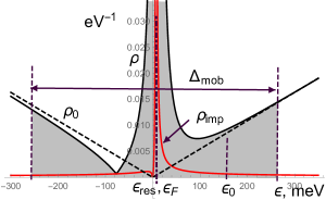
Figure 8: Restructured DOS of graphene under H adatoms (see the AM parameters in Table 1) with concentration $c=0.01$ and symmetric sublattice occupation. The total value $\rho$ (black line) and its impurity component $\rho_{imp}$ (red line) are compared to $\rho_{0}$ of unperturbed graphene (dashed line). The mobility gap $\Delta_{mob}$ range is shadowed.

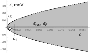
Figure 9: Mobility gaps (shadowed areas bordered by dashed lines) and Fermi level (solid line) vs concentration $c$ of strongly coupled H adatoms, compare with the related DOS in Fig. 8. After the upper $\Delta_{mob}$ gap onsets and absorbs $\varepsilon_{\rm F}$ at extremely low $c_{0}\approx 4\cdot 10^{-6}$, it rapidly merges with the lower $\Delta_{\rm D}$ already at $c_{1}\approx 2\cdot 10^{-3}$.

Also a strong host-impurity coupling modifies the above estimates for the mobility gap near that resonance, making it much broader. Correspondingly, the Fermi level enters it at as low critical concentration as $c_{0}\approx 4\cdot 10^{-6}$, for the H case, and then stays close to the resonance, as shown in Fig. 9. This makes the metallic state extremely unstable against such impurities (within the adopted graphene model with no intrinsic band splitting, e.g., by spin-orbit effects). At last, the strong impurity-host coupling favors to merging of different mobility gaps observed in the weak coupling case, as seen in a rapid absorption of the narrow $\Delta_{\rm D}$ by much broader $\Delta_{mob}$ in Fig. 9 and no traces for decoupling of $\tilde{\Delta}_{mob}$.

Depending on the sign of the on-site energy $\varepsilon_{0}$, the resonance $\varepsilon_{res}$ develops below or above the graphene charge neutrality (Dirac) point. For two considered AM cases, Cu and H, they lie above, and those situations resemble donor-like dopants in common semiconductors—the total carrier weight determining the Fermi level, see Eq. 16, is $Q=1+c>1$. For the case of F, negative $\varepsilon_{0}=-2.2$ eV leads to $\varepsilon_{res}\approx-0.4$ eV, and the whole situation resembles acceptor-like dopants, where the carrier weight turns $Q=1-c<1$. This produces the DOS picture as displayed in Fig. 10, seen qualitatively as a mirror to the cases of donor impurities ($\varepsilon_{0}>0$), and so the restructured spectrum is of inverted type.

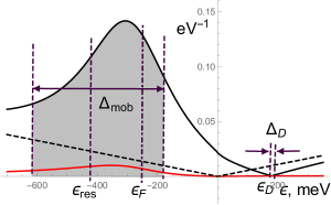
Figure 10: Restructured DOS of graphene under F adatoms with concentration $c=0.03$ and symmetric sublattice occupation (see the model parameters in Table 1). The total value $\rho$ (solid line) is compared to the unperturbed graphene linear DOS, $\rho_{0}$ (dashed line), and two shaded areas present mobility gaps $\Delta_{mob}$, and $\Delta_{\rm D}$.

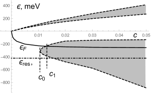
Figure 11: Mobility gaps, bottom $\Delta_{mob}$ and top $\Delta_{\rm D}$ (shadowed areas bordered by dashed lines) and the Fermi level (solid line) vs concentration $c$ of F adatoms in graphene. The localized range $\Delta_{mob}$ onsets near the resonance energy $\varepsilon_{res}\approx-0.4$ eV at the critical concentration $c_{0}\approx 1.06\cdot 10^{-2}$ to absorb the Fermi level at the next critical value $c_{1}\approx 1.3\cdot 10^{-2}$, realizing a robust metal-insulator transition for hole-type charge carriers.

Here, with growing the impurity concentration $c$, the Fermi level goes monotonously down from zero and enters the mobility gap near the impurity resonance at some $c_{1}>c_{0}$, which results in a robust metal-insulator transition for the hole-type charge carriers, see Fig. 11. Those results are in agreement with the experimental findings of Hong et al Hong et al. (2011) that report metal-insulator transition in the fluorinated graphene at certain charge doping levels.

V.4 Asymmetric t-occupancy

Alike that for non-resonant LM impurities, the above discussed effects for AM t-impurities get altered when considering asymmetric sublattice occupations. In this section we only focus on the extreme case corresponding to $c_{1}=c$, $c_{2}=0$.

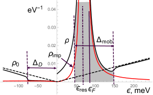
Figure 12: Density of states for graphene with Cu t-impurities at their concentration $c=0.01$ and asymmetric occupation of host sublattices (the same notations used for its elements as in Fig. 6).

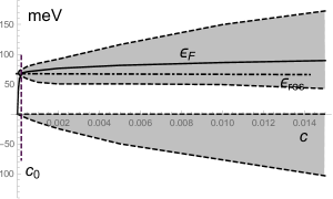
Figure 13: Mobility gaps (shadowed areas bordered by dashed lines) and Fermi level (solid line) vs concentration $c$ for Cu adatoms at asymmetric occupation. Note the difference of mobility gaps development from the case of symmetric occupation in Fig. 7.

Having the related T-matrix: $\hat{T}(\varepsilon)=T_{t}(\varepsilon)\hat{m}_{1}$, the direct evaluation of ${\rm Re}\bigl{[}{\rm Det}\,\hat{G}_{\bf k}^{-1}(\varepsilon)\bigr{]}$ with $\hat{G}_{\bf k}^{-1}(\varepsilon)$ given by Eq. 49 results in the following secular equation:

$$\varepsilon^{2}-\varepsilon_{q}^{2}-2c\,\varepsilon\,{\rm Re\,}\,T_{t}(\varepsilon)=0,$$ (77)

that gives the restructured energy spectrum. Linearizing $T_{t}(\varepsilon)$ in the above expression turns it into the cubic equation with respect to $\varepsilon$, unlike the symmetric t-case governed by Eq. 55. The EPS roots $E_{\alpha,q}$ ($\alpha=1,2,3$) of Eq. 77 can be straightforwardly obtained by the Cardano’s formulas, but their following analyzes turn to be awkward and unpractical. However, the above secular equation also admits an easy and “user-friendly” MPS:

$$q(\varepsilon)=\frac{q_{max}}{W}\sqrt{\varepsilon^{2}-2c\,\varepsilon\,T_{t}(\varepsilon)},$$ (78)

which leads to the corresponding DOS:

$$\rho_{as}(\varepsilon) = \frac{2}{\pi W^{2}}{\rm Im\,}\left\{\left[\varepsilon-c\varepsilon T_{t}(\varepsilon)\right]\right.$$ (79)

$$\times \left.\ln\left[1-\frac{W^{2}}{\varepsilon^{2}-2c\,\varepsilon\,T_{t}(\varepsilon)}\right]\right\},$$

presented in Fig. 12. Its main difference from the symmetric counterpart, Fig. 6, consists in the opening of an effective gap, $\Delta_{\rm D}$, from the initial zero Dirac point to its shifted position, $\varepsilon_{\rm D}\approx-2c\tilde{\omega}^{2}/\varepsilon_{res}$, alike the case of asymmetric occupancy in LM, displayed in Fig. 3. Next, using the MPS by Eq. 78 in the IRM criterion by Eq. 70, one can estimate the underlying mobility gaps, as well near the subband edges as around the resonance peak. The corresponding subbands and mobility gaps are displayed in function of impurity concentration in Fig. 13. From the point of view of metal-insulator transitions, the asymmetric AM scenario offers a richer intermittency between the extended and localized ranges and, along with presence of a wide and almost pure $\Delta_{\rm D}$ gap in its spectrum, it is expected to provide a more promising application-oriented playground than the symmetric case.

VI Anderson’s impurities at bridge and hollow positions

VI.1 Bridge position

Practically the same scenario as for symmetric AM t-impurities is found for AM impurities at b-positions, though this conclusion requires some additional analysis and clarification.

Assume an AM impurity to occupy a b-position projected at ${\bf r}$, then its two neighboring carbon atoms reside at host sites ${\bf n}_{1,i}={\bf r}-{\boldsymbol{\delta}}_{i}/2$ (A sublattice) and ${\bf n}_{2,i}={\bf r}+{\boldsymbol{\delta}}_{i}/2$ (B sublattice), where ${\boldsymbol{\delta}}_{i}$ is one of three nearest neighbor vectors defining the given bridge, see Figs. 1 and 4. The corresponding scattering spinor in the conduction-valence band space, Eq. 37, is explicitly given as:

$$u_{{\bf r},{\bf k}}=\sqrt{2}\,{\rm e}^{i{\bf k}\cdot{\bf r}}\,\left(\begin{array}[]{r}\cos{\tfrac{1}{2}({\bf k}\cdot{\boldsymbol{\delta}}_{i}-\mathrm{arg}\,\gamma_{{\bf k}})}\\ -i\sin{\tfrac{1}{2}({\bf k}\cdot{\boldsymbol{\delta}}_{i}-\mathrm{arg}\,\gamma_{{\bf k}})}\end{array}\right).$$ (80)

Here ${\bf k}$ is referred to the $\Gamma$-point and the hopping factor argument, $\mathrm{arg}\,\gamma_{{\bf k}}$, is given by Eq. 7. This spinor defines the scattering matrix $\hat{V}_{{\bf r},{\bf k},{\bf k}^{\prime}}$, Eq. 41, and then the momentum diagonal T-matrix, Eq. 42, as:

$$\hat{T}_{{\boldsymbol{\delta}}_{i},{\bf k}}(\varepsilon) = T_{t}(\varepsilon)\left[\hat{1}+\hat{\sigma}_{3}\cos{\left({\bf k}\cdot{\boldsymbol{\delta}}_{i}-{\rm arg}\,\gamma_{{\bf k}}\right)}\right.$$ (81)

$$- \left.\hat{\sigma}_{2}\sin{\left({\bf k}\cdot{\boldsymbol{\delta}}_{i}-{\rm arg}\,\gamma_{{\bf k}}\right)}\right],$$

with the same scalar prefactor $T_{t}(\varepsilon)$ as in the t-case, Eq. 45. Assuming also equal average occupancy of three non-equivalent bridge configurations, $c_{{\boldsymbol{\delta}}_{i}}=c/3$, the partial T-matrices $\hat{T}_{{\boldsymbol{\delta}}_{i}}$ combine into the total T-matrix:

$$\hat{T}(\varepsilon,{\bf k})=\frac{1}{3}\sum_{i=1}^{3}\hat{T}_{{\boldsymbol{\delta}}_{i},{\bf k}}(\varepsilon)=\left(\hat{1}+\frac{|\gamma_{{\bf k}}|}{3}\,\hat{\sigma}_{3}\right)T_{t}(\varepsilon).$$ (82)

For momenta ${\bf k}$ close to the graphene valleys centers, ${\bf k}={\bf q}+{\bf K}^{(\prime)}$, one can employ the low-energy expansion to present the T-matrix for b-impurities as:

$$\hat{T}(\varepsilon,q)=\left(\hat{1}+\frac{\varepsilon_{q}}{3t}\,\hat{\sigma}_{3}\right)T_{t}(\varepsilon),$$ (83)

thus dependent on the radial component $q$ of reduced momentum. But in the long-wave limit, $\varepsilon_{q}\ll W\sim 3t$, the momentum dependent term in Eq. 83 can be practically neglected. Therefore in the considered low-energy limit, the b-case T-matrix gets effectively reduced just to $T_{t}(\varepsilon)\hat{1}$. As a consequence, the restructured energy spectrum in the presence of b-impurities should mostly reproduce the same spectral features as for the symmetric t-case.

To what types of adatoms on graphene one can apply the above findings? First-principle calculations predict oxygen and nitrogen to bond in the bridge position Wu et al. (2008). However, also for some top positioned impurities, like copper Wu et al. (2009); Amft et al. (2011); Frank et al. (2017), and gold Chan et al. (2008); Amft et al. (2011) the energy difference between the top and bridge configurations is relatively small, and therefore their bridge realization can become probable. Similarly, the light ad-molecules like CO, NO and NO₂ prefer to adsorb Leenaerts et al. (2008) equally-likely to the hollow and bridge positions.

VI.2 Hollow position

Hollow-type AM impurities represent a special case; an adatom in the h-position displays local $C_{6v}$ symmetry, which strongly reduces the coupling of impurity degrees of freedom with host graphene states (see Eq. 85 below). That was earlier interpreted as their full decoupling Ruiz-Tijerina and da Silva (2016) from graphene states. However, it will be shown below that, when treated consistently within the AM, the h-impurities are sufficient to produce essential restructuring of graphene low-energy spectrum. The resulting h-type resonances and the related spectral features in terms of AM parameters are compared in what follows with the previously discussed t- and b-cases.

For an h-impurity projected to ${\bf r}$, the sum in the scattering spinor $u_{{\bf r},{\bf k}}$, Eq. 37, counts its 6 carbon neighbors. Those are residing at host sites: ${\bf n}_{1,i}={\bf r}+{\boldsymbol{\delta}}_{i}$ (A sublattice), and ${\bf n}_{2,i}={\bf r}-{\boldsymbol{\delta}}_{i}$ (B sublattice, see Figs. 1 and 4). This summation results in:

$$u_{{\bf r},{\bf k}}=\sqrt{2}\,|\gamma_{{\bf k}}|\,{\rm e}^{i{\bf k}\cdot{\bf r}}\left(\begin{array}[]{r}\cos{\bigl{(}\tfrac{3}{2}\,\mathrm{arg}\,\gamma_{{\bf k}}\bigr{)}}\\ i\sin{\bigl{(}\tfrac{3}{2}\,\mathrm{arg}\,\gamma_{{\bf k}}\bigr{)}}\end{array}\right).$$ (84)

Implementing this into Eq. 42 leads to the corresponding momentum diagonal T-matrix:

$$\hat{T}_{{\bf r},{\bf k}}(\varepsilon) = T_{h}(\varepsilon)\,|\gamma_{{\bf k}}|^{2}\,\Bigl{[}\hat{1}+\hat{\sigma}_{3}\cos{\left(3\,\mathrm{arg}\,\gamma_{{\bf k}}\right)}$$ (85)

$$\qquad+\hat{\sigma}_{2}\sin{\left(3\,\mathrm{arg}\,\gamma_{{\bf k}}\right)}\Bigr{]}.$$

where the scalar prefactor $T_{h}(\varepsilon)=\omega^{2}/D(\varepsilon)$ differs from $T_{t}(\varepsilon)$, Eq. 45, by more complex denominator:

$$D(\varepsilon)=\varepsilon-\varepsilon_{0}+\frac{2\varepsilon\omega^{2}}{t^{2}}\bigl{[}1-\varepsilon G^{(0)}(\varepsilon)\bigr{]}.$$ (86)

Similarly to the b-case, Eq. 83, the h-impurity T-matrix, Eq. 85, depends apart of the radial momentum $q$, also on its azimuthal component encoded in $\mathrm{arg}\,\gamma_{{\bf k}}$. This makes the restructured dispersion relation based on Eq. 85 anisotropic. Another important difference of the h-case T-matrix from the t- and b-cases is in the small prefactor, $|\gamma_{{\bf q}+{\bf K}^{(\prime)}}|^{2}\approx(\varepsilon_{q}/t)^{2}\ll 1$, in its numerator, which is responsible for the above mentioned decoupling of the graphene low-energy states with h-type AM impurities. The complete low-energy T-matrix for momenta near the ${\bf K}^{(\prime)}$ point reads:

$$\hat{T}(\varepsilon,{\bf q})=T_{h}(\varepsilon)\frac{\varepsilon_{q}^{2}}{t^{2}}\Bigl{[}\hat{1}\mp\hat{\sigma}_{3}\cos{\left(3\theta_{\bf q}\right)}-\hat{\sigma}_{2}\sin{\left(3\theta_{\bf q}\right)}\Bigr{]},$$ (87)

where the plus (minus) sign applies to ${\bf K}^{(\prime)}$ valley, and the form of angle $\theta_{\bf q}$ is given by Eq. 7.

The general formulas, Eqs. 85-87, allow to study, at least numerically, the spectral effects of h-type AM impurities in a broad energy range. However, in what follows we stay rather on analytical side, using proper approximations near the Dirac points. For example, to find the resonance pole of T-matrix and the restructured dispersion laws over the low-energy range, $(\varepsilon/t)^{2}\ll 1$, it is well justified to ignore the strongly suppressed $G^{(0)}(\varepsilon)$ term in the denominator $D(\varepsilon)$, which can be then approximated by $D(\varepsilon)\approx\varepsilon-\varepsilon_{0}+2\varepsilon\omega^{2}/t^{2}$. The correspondingly approximated $T_{h}(\varepsilon)\approx\tilde{\omega}^{2}/(\varepsilon-\varepsilon_{res})$ involves the resonance level:

$$\varepsilon_{res}\approx\frac{\varepsilon_{0}}{1+2(\omega/t)^{2}},$$ (88)

and the effective coupling constant $\tilde{\omega}^{2}=\omega^{2}t^{2}/(t^{2}+2\omega^{2})$. Then the secular equation, Eq. 51, takes the form of an ordinary cubic equation:

$$\varepsilon^{2}-\varepsilon_{q}^{2}\left(1+\tilde{c}\,\frac{\varepsilon-\varepsilon_{q}\cos 3\theta_{\bf q}}{\varepsilon-\varepsilon_{res}}\right)=0,$$ (89)

with $\tilde{c}=2c(\tilde{\omega}/t)^{2}$. As noted above, the resulting dispersion is anisotropic, and the angular $\cos 3\theta_{\bf q}$ dependence imprints the spectrum near $\varepsilon_{res}$ the $C_{3}$ symmetry. In sequel we characterize that general spectrum by its behavior along the basic directions in the momentum plane: the nodal with $\cos 3\theta_{\bf q}=0$, and the anti-nodal with $\cos 3\theta_{\bf q}=\pm 1$. The main features for each considered case are shown in Fig. 14 and can be summarized as follows.

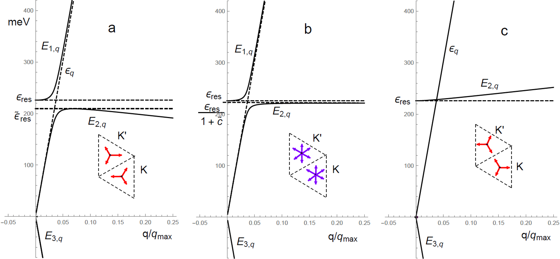
Figure 14: Restructured electronic dispersion of graphene in the presence of h-positioned impurities with $\varepsilon_{res}\approx 226$ meV, $\omega=t/\sqrt{2}$, and concentration $c=0.02$, along the nodal (blue arrows) and anti-nodal (red arrows) directions in the BZ with respect to ${\bf K}$ and ${\bf K}^{(\prime)}$ points, see insets.

i) Along the anti-nodal directions: $\theta_{\bf q}=\pi,\pm\pi/3$ around the ${\bf K}$-point and $\theta_{\bf q}=0,\pm 2\pi/3$ around the ${\bf K}^{\prime}$-point (red arrows in Fig. 14a), the restructured spectra:

$$E_{{}^{1}_{2},{\bf q}} = \frac{\varepsilon_{res}+\varepsilon_{q}\pm\sqrt{(\varepsilon_{res}-\varepsilon_{q})^{2}+4\tilde{c}\varepsilon_{q}^{2}}}{2},$$

$$E_{3,{\bf q}} = -\varepsilon_{q},$$ (90)

include the purely unperturbed valence graphene band $-\varepsilon_{q}$, and the restructured $E_{{}^{1}_{2},q}$ bands. They emerge from the spectral repulsion between the graphene conduction band $\varepsilon_{q}$ and the resonance level $\varepsilon_{res}$ (supposing for definiteness $\varepsilon_{res}>0$). The most notable features here are the formation of a wider quasi-gap (anti-crossing) between $\varepsilon_{res}$ and $\tilde{\varepsilon}_{res}=\varepsilon_{res}/(1+4\tilde{c})$ and the inverted group velocity of $E_{2,q}$ at $\varepsilon_{q}>2\tilde{\varepsilon}_{res}$. This is due to the $q^{2}$-growth of the effective impurity-host coupling. Inverted group velocity generates also lower impurity side-band $W_{imp}\approx\tilde{c}W$, see Figs. 15 and 16, which is still broad enough compared to the related mobility gap $\Delta_{mob}$.

ii) Along the nodal directions: $\theta_{\bf q}=\pm\pi/6$, $\pm\pi/2$, $\pm 5\pi/6$ (shown by blue arrows around each ${\bf K}$-point in Fig. 14b), the cubic equation, Eq. 89, promotes couplings of the resonance level $\varepsilon_{res}$ to both graphene $\pm\varepsilon_{\bf q}$ bands. On one side the strong interaction of $\varepsilon_{res}$ with the conduction band $\varepsilon_{q}$ produces two restructured bands, $E_{{}^{1}_{2},q}$, with a very narrow anti-crossing between their asymptotic limits $E_{1,0}=\varepsilon_{res}$ and $E_{2,q_{max}}=\varepsilon_{res}/(1+\tilde{c})$. Contrary, a weak non-resonant coupling of $\varepsilon_{res}$ with the valence band $-\varepsilon_{q}$ results only in slight modification of the latter, band $E_{3,q}$.

iii) Along the inverted anti-nodal directions: $\theta_{\bf q}=0,\pm 2\pi/3$ around the ${\bf K}$-point and $\theta_{\bf q}=\pi,\pm\pi/3$ around the ${\bf K}^{\prime}$-point (red arrows in Fig. 14c), these spectra:

$$E_{1,{\bf q}} = \varepsilon_{q},$$

$$E_{{}^{2}_{3},{\bf q}} = \frac{\varepsilon_{res}-\varepsilon_{q}\pm\sqrt{(\varepsilon_{res}+\varepsilon_{q})^{2}+4\tilde{c}\varepsilon_{q}^{2}}}{2},$$ (91)

include the purely unperturbed graphene conduction band $\varepsilon_{q}$, and subbands $E_{2,q}$ and $E_{3,q}$ that originate from a non-resonant repulsion between $-\varepsilon_{q}$ and $\varepsilon_{res}$. Subband $E_{2,q}$ has the width $W_{imp}^{\prime}$, see Figs. 15 and 16, and the valence $E_{3,q}$ only slightly deviates from the original valence band $-\varepsilon_{q}$.

Another peculiarity here is the absence of the shift of the energy level for the Dirac point that was present as $\varepsilon_{\rm D}\neq 0$ in the previous cases. Also peculiar DOS features appear near the impurity resonance, as shown in Fig. 15, with their notable differences from the t- and b-cases. First, in practical vanishing of quasi-gap (due to the same small prefactor in the impurity-host coupling as indicated before Eq. 87) and second, in the appearance of new side-bands around $\varepsilon_{res}$ with widths $\approx\tilde{c}W$, that can be seen as the “impurity induced heavy fermions” with an emergent $f$-wave symmetry. The details of analytic calculation of this DOS function are given in Appendix B.

The resulting sum of the DOS components, $\rho_{host}(\varepsilon)=\pi^{-1}{\rm Im}\,g(\varepsilon)$ and $\rho_{imp}={\rm Im}\,T_{h}(\varepsilon)$ presented in Fig. 15 reveals its contributions from the spectrum branches $E_{{}^{1}_{2},{\bf q}}$ with a spike at $\varepsilon_{res}$ and a break at $\tilde{\varepsilon}_{res}$.

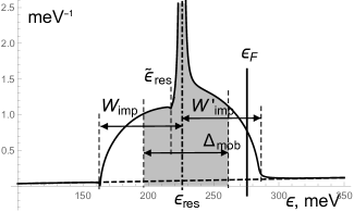
Figure 15: DOS due to h-position impurities with AM parameters as in Fig. 14. The resonance peak at $\varepsilon_{res}$ is bordered from both sides by much wider impurity side-bands $W_{imp}$ and $W^{\prime}_{imp}$. The localized states within the mobility gap $\Delta_{mob}$ are shadowed, the unperturbed DOS $\rho_{0}(\varepsilon)$ is shown by the dashed line.

The obtained dispersions and DOS can be further used for the IRM criterion, Eq. 70, and for comparing the Fermi level and mobility edge positions. In this approach, the dispersion equation in its complete form:

$$\varepsilon^{2}-\varepsilon_{q}^{2}\left[1+\frac{2c\omega^{2}}{t^{2}}\frac{\varepsilon-\varepsilon_{q}\cos 3\theta_{\bf q}}{D(\varepsilon)}\right]=0$$ (92)

(instead of simplified Eq. 89), can provide an MPS $q(\varepsilon,\theta)$ along a given azimuthal direction $\theta=\theta_{\bf q}$. Then the related mobility edges can be estimated numerically from an extension of Eq. 70:

$${\rm min}_{\theta}\,\left|\frac{{\rm Re}\,q(\varepsilon,\theta)}{\partial{\rm Re}\,q(\varepsilon,\theta)/\partial\varepsilon}\right|=\hbar\tau^{-1}(\varepsilon),$$ (93)

where, from symmetry considerations, the minimum is sought along the above defined nodal and anti-nodal directions. Their comparison, readily, indicates such minimum to be along the anti-nodal directions displayed in Fig. 14a (with $\cos 3\theta_{\bf q}=-1$ and the widest quasi-gap). The corresponding explicit solution of Eq. 92 reads:

$$q_{0}(\varepsilon)=q_{max}\frac{\sqrt{D(\varepsilon)\left(D(\varepsilon)+4c\varepsilon\right)}-D(\varepsilon)}{2cW},$$ (94)

and using it in Eq. 93 gives finally the mobility edges as shown in Fig. 16.

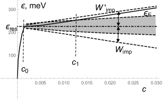
Figure 16: Development of the mobility gap $\Delta_{mob}$, impurity side-bands $W_{imp}$ and $W^{\prime}_{imp}$ and Fermi level $\varepsilon_{\rm F}$ vs concentration $c$ for h-position impurities with AM parameters as in Figs. 14, 15.

In similarity to the before considered t-cases displayed in Figs. 7, 9, 11, 13, here a localized range emerges near $\varepsilon_{res}$ at the critical concentration $c_{0}\approx 1.5\cdot 10^{-3}$, and then extends further sublinearly in $c$, see the shadowed area in Fig. 16. Its limits are exceeded from below and above by the linearly growing outer side-bands $W_{imp}$ and $W^{\prime}_{imp}$ (dashed lines) that contain extended “heavy fermionic” states, see also the DOS displayed in Fig. 15. In this course, the Fermi level $\varepsilon_{\rm F}$ rises from zero through the initial conduction band $\varepsilon_{q}$ and then enters into the mobility gap at $c\approx c_{0}$. Further, with grown $c$ the Fermi level leaves that localized region at another critical concentration $c_{1}\approx 0.013$, and penetrates into the $W^{\prime}_{imp}$ side-band with the “heavy fermionic” character. Thus h-type AM impurities realize both metal/insulator and insulator/metal transitions, but the two metallic phases are different, the initial is $s$-like and the later is $f$-like. Thus, the h-type adatoms can be considered, together with the asymmetric t-ones, as the most prospective candidates for possible applications.

Ab-initio studies are unveiling that light metallic adatoms Chan et al. (2008) from groups I-III and also heavy transition metals Chan et al. (2008); Weeks et al. (2011b); Mao et al. (2008) are favored for adsorption above the centers of graphene hexagons, i.e. at hollow positions. The same is true for light ad-molecules like NH₃, H₂O, NO₂ Leenaerts et al. (2008).

VII Discussion

The presented results demonstrate several characteristic tendencies that can accompany spectral transformation of the electronic band structure of graphene in the presence of disorder produced by impurities. The first decisive factor in that process is to understand whether a single impurity center can produce a resonance energy level in the spectrum. The affirmative answer is imposing some additional restrictions on the strengths of hybridization parameter and on-site energy. As demonstrated above, this is practically always granted within the scope of Anderson hybrid model, reasonably justified for most of common adatoms (ad-molecules) chemisorbed at graphene layer, and less granted for the isotopic Lifshitz model.

Once a resonance level exists for a given impurity type, by increasing their concentration the graphene spectrum would restructuralize following a particular scenario. The later is determined by the impurity locations [top, bridge, or hollow], and by their sublattice occupations [symmetric or asymmetric]. The most important spectral changes are emergencies of particular localized ranges and (pseudo)gaps that pop out inside the initial continuum of band states. Typically near the original resonance level, and also near the restructured Dirac points. Their further development with increased concentration is conveyed by splittings or mergings, as manifested by the fate of mobility edges that come from the phenomenological IRM criterion. It should be yet noted that such localized ranges and related mobility gaps in the spectrum can also arise from a specific braking of the sublattice occupation of graphene due to impurities, even, in the absence of single impurity resonance. Due to its simplicity, the latter mechanism can be especially helpful in the search for practical realizations of properly restructured spectra.

The underlying electronic phase [metallic or insulating] of the resulting physical system is then essentially determined by the position of the Fermi level relative to the localized ranges. Those imprint the impurity type and concentration, but could be yet tuned by the external means, namely, electric or magnetic bias, temperature, etc., opening a wide field for possible applications. Compared to the common situation in doped semiconductors, this provides much more versatile possibilities for interchange of different types of metallic and insulating states, and mutual transitions among them. Also, in this course, there are possibilities to combine the several spectral effects originating from different impurity species simultaneously, and thus target different energy ranges. However, the presented analysis did not consider the situation when randomly distributed impurities at low concentration nucleate in nearest neighbor positions forming impurity clusters. Those in reality exist (as known for some dopants in common semiconductors), and such direct impurity-impurity coupling will produce split resonances and, correspondingly, more complicated series of localized energy ranges around them.

Finally, besides the purely electronic properties the variety of spectral regimes permits also other notable effects that employ additional degrees of freedom as, for instance, collective plasmonic spectra by narrow conduction bands, optical susceptibility by narrow insulating gaps, Hall effect and magneto-transport on anisotropic Fermi surface, etc. From the above analysis the promising impurity types are weakly coupled t-position adatoms (including their donor-acceptor combinations) and h-position hybridizing species (admitting a wider range of their atomic levels and coupling parameters).

The approach as presented, and the list of impurity effects that count the simplest host, single-layer graphene, can be further substantially developed in several different directions, for example, to multilayered graphene and its hexagonal lattice analogs, topological edge states, and quantum Hall effect regimes, Moiré patterns from plane rotations, etc. Such systems can present new playground for probing the interplay between the impurity disorder/localization effects, and the symmetry/topology order protection.

VIII Acknowledgements

The work of VML was partially supported by the Ukrainian-Israeli Scientific Research Program of the Ministry of Education and Science of Ukraine and the Ministry of Science and Technology of the State of Israel, as well as by Grant Nos. 0117U000236 and 0117U000240 from the Department of Physics and Astronomy of the National Academy of Sciences of Ukraine. DK acknowledges support from Deutsche Forschungsgemeinschaft, Project-ID 314695032 (SFB 1277), and the EU Seventh Framework Programme under Grant Agreement No. 604391 (Graphene Flagship).

Appendix A Group expansion analysis

The above analysis was based on the impurity averaged GF’s within the simplest T-matrix approximation. Generally, one needs to check the higher order of GE (in powers of $c$) for the self-energy, Eq. 27, and their potential impact on the formerly obtained results. Here the principal point is the convergence criterion for GE series, justifying its approximation by the T-matrix term. In what follows we provide estimates for the first non-trivial pair term of GE, giving a self-energy correction to the second order in $c$. We approximate the convergence criterion as:

$$c|B_{\bf q}|<1.$$ (95)

It should be noted that, due to $j$-orthogonality of the scattering matrices $\hat{m}_{j}$, Eq. 25, such pair scatterings contribute to the momentum diagonal GF only for t-impurities belonging to the same $j$-th sublattice. Therefore, the total self-energy matrix for the momentum-diagonal GF results to be additive in the sublattice $j$-indices:

$$\hat{G}_{\bf q}^{-1}=\left(\hat{G}_{\bf q}^{(0)}\right)^{-1}-\sum_{j}c_{j}\hat{m}_{j}\Sigma_{j,{\bf q}}.$$

Each $j$-th sublattice self-energy $\Sigma_{j,{\bf q}}$ has its own GE, analogous to general Eq. 27, with the corresponding pair term, $c_{j}B_{\bf q}$, whose scalar B-factor is explicitly given as follows Lifshitz et al. (1988):

$$B_{{\bf q}}(\varepsilon)=\sum_{{\bf n}\neq 0}\frac{{\rm e}^{-i{\bf q}\cdot{\bf n}}A_{\bf n}(\varepsilon)+A_{\bf n}(\varepsilon)A_{-{\bf n}}(\varepsilon)}{1-A_{\bf n}(\varepsilon)A_{-{\bf n}}(\varepsilon)}.$$ (96)

This sum describes all multiple scatterings on impurity pairs from the same sublattice separated by lattice vectors ${\bf n}\neq 0$ (measured in units of graphene lattice constant $a$), returning a quasiparticle to its initial ${\bf q}$-state, through the dimensionless correlator:

$$A_{{\bf n}}(\varepsilon)=\frac{T_{t}(\varepsilon)}{N}\sum_{{\bf k}}{\rm e}^{i{\bf k}\cdot{\bf n}}\,{\rm Tr}\,\hat{G}_{{\bf k}}^{(0)}(\varepsilon).$$ (97)

The later can be presented as a product:

$$A_{{\bf n}}(\varepsilon)=T_{t}(\varepsilon)\sigma_{\bf n}f_{\bf n}(\varepsilon),$$

where the factor $\sigma_{\bf n}=({\rm e}^{i{\bf K}\cdot{\bf n}}+{\rm e}^{i{\bf K}^{\prime}\cdot{\bf n}})/2$ takes the values 1, $z={\rm e}^{2i\pi/3}$ and $z^{\ast}$ with the host lattice periodicity, as a consequence $\sigma_{\bf n}\sigma_{-{\bf n}}=1$ (see Fig. 17).

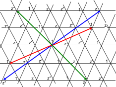
Figure 17: Distribution of $\sigma_{\bf n}$ values 1, $z={\rm e}^{2i\pi/3}$ and $z^{\ast}$ over lattice sites (from the same $j$-sublattice) with examples of their products in opposite pairs (with respect to an initial zero site) to satisfy $\sigma_{\bf n}\sigma_{-{\bf n}}=1$.

The remaining sum over the reduced momentum reads:

$$f_{\bf n}(\varepsilon)=\frac{1}{N}\sum_{{\bf q}}{\rm e}^{i{\bf q}\cdot{\bf n}}\,{\rm Tr}\,\hat{G}_{{\bf q}}^{(0)}(\varepsilon),$$ (98)

what can be routinely approximated by the following integral (see also Eq. 8):

$$f_{\bf n}(\varepsilon) \approx \frac{4\varepsilon}{q_{max}^{2}}\int_{0}^{q_{max}}\frac{J_{0}(qn)qdq}{\varepsilon^{2}-\varepsilon_{q}^{2}}$$ (99)

$$\approx \frac{4\varepsilon}{q_{max}^{2}}\int_{0}^{\infty}\frac{J_{0}(qn)qdq}{\varepsilon^{2}-\varepsilon_{q}^{2}}$$

$$= -\frac{4\varepsilon}{W^{2}}K_{0}\left(i\frac{n}{n_{\varepsilon}}\right).$$

Here the length scale is set by $n_{\varepsilon}=q_{max}^{-1}W/\varepsilon$, so for $n\gtrsim n_{\varepsilon}$ we have $q_{max}n\gg 1$ and it is justified to extend the integration limit to infinity, transforming the Bessel function $J_{0}$ into the Macdonald function $K_{0}$ we can employ its asymptotics: $K_{0}(ix)\approx\sqrt{i\pi/(2x)}\,{\rm e}^{-ix}$ for $x\gg 1$, see Abramowitz and Stegun (1964).

Using the above results, and summing over ${\bf n}$, Eq. 96, we can take into account that $f_{\bf n}$ in $A_{{\bf n}}$ varies very slowly at the lattice scales, $n\sim a\sim q_{max}^{-1}$ (as well as ${\rm e}^{i{\bf q}\cdot{\bf n}}$ at $q\ll q_{max}$), so that averaging of $\sigma_{{\bf n}}$ follows the rules: $\langle\sigma_{{\bf n}}\rangle=0$, $\langle\sigma_{{\bf n}}\sigma_{-{\bf n}}\rangle=1$. This makes the contribution of the first term in the numerator negligible compared to the second one. The resulting expression of $B_{\bf q}$ turns to be already ${\bf q}$-independent, i.e. $B_{\bf q}\approx B$, where

$$B\approx-\frac{4\pi n_{\varepsilon}^{2}z_{\varepsilon}}{\sqrt{3}a^{2}}\int_{0}^{\infty}\frac{xdx}{z_{\varepsilon}-ix{\rm e}^{2ix}},$$ (100)

with $z_{\varepsilon}=\tfrac{32}{3}(\pi\varepsilon T_{h}(\varepsilon)/W^{2})^{2}$. The numerical estimate for the integral in Eq. 100 in assumption of $|z_{\varepsilon}|\lesssim 1$ shows its absolute value to be $\sim 1$, then the corresponding criterion for GE convergence follows as:

$$c\frac{4\pi n_{\varepsilon}^{2}z_{\varepsilon}}{\sqrt{3}a^{2}}\lesssim 1.$$ (101)

This gives an estimate for the GE convergence range:

$$|\varepsilon-\varepsilon_{res}|\gtrsim c^{1/2}\frac{\tilde{\omega}^{2}}{W}.$$ (102)

This is deep within the mobility gap estimated in the T-matrix approximation, Eq. 74, so the higher order GE terms cannot influence the formerly established results stemming solely from the T-matrix. Also the above assumed condition of $|z_{\varepsilon}|\lesssim 1$ is well confirmed in the range by Eq. 102.

Appendix B DOS calculation for hollow position impurities

In the presence of h-type AM impurities, the DOS, more precisely the part dominated by the host bands, is conventionally obtained from Eq. 14. For that one would need the perturbed GF, Eqs. 26 and 27, that can be in the lowest order in $c$ obtained with the help of the T-matrix, for its the explicit form see Eq. 87. Taking all that on gets for the trace of the locator of the perturbed GF, ${\rm Tr\,}\hat{G}_{loc}(\varepsilon)\equiv g(\varepsilon)$, the following expression

$$g(\varepsilon) =\frac{2}{\pi q_{max}^{2}}\,\int_{0}^{2\pi}d\theta\int_{0}^{q_{max}}qdq$$ (103)

$$\times\frac{\varepsilon D-\tilde{c}\varepsilon_{q}^{2}}{\left(\varepsilon^{2}-\varepsilon_{q}^{2}\right)D-\tilde{c}\varepsilon_{q}^{2}\left(\varepsilon-\varepsilon_{q}\cos\theta\right)},$$

where $D=D(\varepsilon)$ is given by Eq. 86. The integral over the azimuthal variable $3\theta_{\bf q}$ was substituted by $\theta$ and when taking into account also the shift of the upper limit it gives what is stated above. The angular integration over $\theta$ can be carried out with the help of the standard formula:

$$\int_{0}^{2\pi}\frac{d\theta}{a-b\cos{\theta}}=\frac{2\pi}{\sqrt{a^{2}-b^{2}}}.$$

The radial integration over $q$ can be processed in terms of the new variable $x=\varepsilon_{q}^{2}$:

$$g(\varepsilon)=\frac{2}{W^{2}}\,\int_{0}^{W^{2}}\frac{\left(\varepsilon D-\tilde{c}x\right)dx}{\sqrt{(\varepsilon^{2}-x)(x-x_{1})(x-x_{2})}},$$ (104)

where the energy dependent roots in the denominator count:

$$x_{1,2}=\frac{D+2\tilde{c}\varepsilon\pm\sqrt{D(D+4\tilde{c}\varepsilon)}}{2\tilde{c}^{2}}.$$

The above integral, Eq. 104, can be calculated analytically, after passing from $x$ to the trigonometric variable $u$:

$$u=\arcsin{\frac{2x-x_{1}-x_{2}}{x_{1}-x_{2}}},$$

and results in:

$$g(\varepsilon) = \frac{\sqrt{x_{1}-x_{2}}}{W^{2}}\,\int_{u_{1}}^{u_{2}}\frac{(\sin u+\alpha_{1})du}{\sqrt{\sin u+\alpha_{2}}}$$ (105)

$$= \frac{2\sqrt{x_{1}-x_{2}}}{W^{2}}\left\{\frac{\alpha_{2}-\alpha_{1}}{\sqrt{1+\alpha_{2}}}\left[F\left(\frac{u_{2}}{2}|\frac{2}{1+\alpha_{2}}\right)\right.\right.$$

$$- \left.F\left(\frac{u_{1}}{2}|\frac{2}{1+\alpha_{2}}\right)\right]-\sqrt{1+\alpha_{2}}\left[E\left(\frac{u_{2}}{2}|\frac{2}{1+\alpha_{2}}\right)\right.$$

$$\qquad\qquad\qquad\left.\left.-E\left(\frac{u_{2}}{2}|\frac{2}{1+\alpha_{2}}\right)\right]\right\}.$$

Here $F(x|y)$ and $E(x|y)$ are, respectively, the elliptic integrals of the 1st and 2nd kind Abramowitz and Stegun (1964) and their arguments include the energy dependent terms:

$$\alpha_{1} =\sqrt{\frac{2D}{D+4\tilde{c}\varepsilon}}, u_{1} =\arccos\frac{2W^{2}-x_{1}-x_{2}}{x_{1}-x_{2}},$$

$$\alpha_{2} =\frac{x_{1}+x_{2}-2\varepsilon^{2}}{x_{1}-x_{2}}, u_{2} =\arccos\frac{x_{1}+x_{2}}{x_{2}-x_{1}}.$$

The result of Eq. 105 permits analytic approximations for the host part of DOS,

$$\rho_{h}(\varepsilon)=\frac{1}{\pi}{\rm Im}\,g(\varepsilon),$$

and, then, similarly for the impurity part of DOS:

$$\rho_{imp}(\varepsilon)=\frac{1}{\pi}{\rm Im}\left[\,\frac{c}{\varepsilon-\varepsilon_{0}-\left(\omega\varepsilon/t\right)^{2}g(\varepsilon)}\right].$$

The resulting total DOS, $\rho_{tot}(\varepsilon)=\rho_{h}(\varepsilon)+\rho_{imp}(\varepsilon)$, is presented in Fig. 15. It clearly displays the contributions from the spectrum branches $E_{{}^{1}_{2},{\bf q}}$ with van Hove singularities at their special energies $\varepsilon_{res}$ and $\tilde{\varepsilon}_{res}$ and practically restores the unperturbed $\rho_{0}(\varepsilon)$ when going with energy beyond the impurity bands that own widths $W_{imp}$ and $W^{\prime}_{imp}$.

References

- Adam et al. (2007) S. Adam, E. H. Hwang, V. M. Galitski, and S. Das Sarma, Proc. Natl. Acad. Sci. USA 104, 18392 (2007).
- Swartz et al. (2013) A. G. Swartz, J.-R. Chen, K. M. McCreary, P. M. Odenthal, W. Han, and R. K. Kawakami, Phys. Rev. B 87, 075455 (2013).
- Jia et al. (2015) Z. Jia, B. Yan, J. Niu, Q. Han, R. Zhu, D. Yu, and X. Wu, Phys. Rev. B 91, 085411 (2015).
- Chandni et al. (2015) U. Chandni, E. A. Henriksen, and J. P. Eisenstein, Phys. Rev. B 91, 245402 (2015).
- Pereira et al. (2006) V. M. Pereira, F. Guinea, J. M. B. Lopes dos Santos, N. M. R. Peres, and A. H. Castro Neto, Phys. Rev. Lett. 96, 036801 (2006).
- Pereira et al. (2008) V. M. Pereira, J. M. B. Lopes dos Santos, and A. H. Castro Neto, Phys. Rev. B 77, 115109 (2008).
- Nanda et al. (2012) B. R. K. Nanda, M. Sherafati, Z. S. Popović, and S. Satpathy, New J. Phys. 14, 083004 (2012).
- Stauber et al. (2007) T. Stauber, N. M. R. Peres, and F. Guinea, Phys. Rev. B 76, 205423 (2007).
- Ferreira et al. (2011) A. Ferreira, J. Viana-Gomes, J. Nilsson, E. R. Mucciolo, N. M. R. Peres, and A. H. Castro Neto, Phys. Rev. B 83, 165402 (2011).
- Monteverde et al. (2010) M. Monteverde, C. Ojeda-Aristizabal, R. Weil, K. Bennaceur, M. Ferrier, S. Guéron, C. Glattli, H. Bouchiat, J. N. Fuchs, and D. L. Maslov, Phys. Rev. Lett. 104, 126801 (2010).
- Robinson et al. (2008) J. P. Robinson, H. Schomerus, L. Oroszlány, and V. I. Fal’ko, Phys. Rev. Lett. 101, 196803 (2008).
- Lee et al. (2019) J. Lee, D. Kochan, and J. Fabian, Phys. Rev. B 99, 035412 (2019).
- Basko (2008) D. M. Basko, Phys. Rev. B 78, 115432 (2008).
- Wehling et al. (2007a) T. O. Wehling, A. V. Balatsky, M. I. Katsnelson, A. I. Lichtenstein, K. Scharnberg, and R. Wiesendanger, Phys. Rev. B 75, 125425 (2007a).
- Skrypnyk and Loktev (2006) Y. V. Skrypnyk and V. M. Loktev, Phys. Rev. B 73, 241402 (2006).
- Ihnatsenka and Kirczenow (2011) S. Ihnatsenka and G. Kirczenow, Phys. Rev. B 83, 245442 (2011).
- Wehling et al. (2010a) T. O. Wehling, H. P. Dahal, A. I. Lichtenstein, M. I. Katsnelson, H. C. Manoharan, and A. V. Balatsky, Phys. Rev. B 81, 085413 (2010a).
- Wehling et al. (2010b) T. O. Wehling, S. Yuan, A. I. Lichtenstein, A. K. Geim, and M. I. Katsnelson, Phys. Rev. Lett. 105, 056802 (2010b).
- Wehling et al. (2007b) T. O. Wehling, A. V. Balatsky, M. I. Katsnelson, A. I. Lichtenstein, K. Scharnberg, and R. Wiesendanger, Phys. Rev. B 75, 125425 (2007b).
- Farjam et al. (2011) M. Farjam, D. Haberer, and A. Grüneis, Phys. Rev. B 83, 193411 (2011).
- Gmitra et al. (2013) M. Gmitra, D. Kochan, and J. Fabian, Phys. Rev. Lett. 110, 246602 (2013).
- Zollner et al. (2016) K. Zollner, T. Frank, S. Irmer, M. Gmitra, D. Kochan, and J. Fabian, Phys. Rev. B 93, 045423 (2016).
- Frank et al. (2017) T. Frank, S. Irmer, M. Gmitra, D. Kochan, and J. Fabian, Phys. Rev. B 95, 035402 (2017).
- Ruiz-Tijerina and da Silva (2016) D. A. Ruiz-Tijerina and L. G. G. V. D. da Silva, Phys. Rev. B 94, 085425 (2016).
- Uchoa et al. (2014) B. Uchoa, L. Yang, S.-W. Tsai, N. M. R. Peres, and A. H. Castro Neto, New J. Phys. 16, 013045 (2014).
- Weeks et al. (2011a) C. Weeks, J. Hu, J. Alicea, M. Franz, and R. Wu, Phys. Rev. X 1, 021001 (2011a).
- Duffy et al. (2016) J. Duffy, J. Lawlor, C. Lewenkopf, and M. S. Ferreira, Phys. Rev. B 94, 045417 (2016).
- Irmer et al. (2018) S. Irmer, D. Kochan, J. Lee, and J. Fabian, Phys. Rev. B 97, 075417 (2018).
- Lifshitz et al. (1988) I. M. Lifshitz, S. A. Gredescul, and L. A. Pastur, Introduction to the Theory of Disordered Systems (Wiley-VCH, Berlin, 1988), ISBN 978-0471875338.
- Anderson (1961) P. W. Anderson, Phys. Rev. 124, 41 (1961).
- Bonch-Bruevich and Tyablikov (2015) V. L. Bonch-Bruevich and S. N. Tyablikov, The Green Function Method in Statistical Mechanics (Dover Publications, 2015), ISBN 9780486797151.
- Economou (2006) E. N. Economou, Green’s Functions in Quantum Physics (Springer-Verlag Berlin Heidelberg, 2006), ISBN 9783540288381.
- Lifshitz (1964) I. M. Lifshitz, Adv. Phys. 13(52), 483 (1964).
- Skrypnyk and Loktev (2018) Y. V. Skrypnyk and V. M. Loktev, Low. Temp. Phys. 44, 1112 (2018).
- Ivanov et al. (1987) M. A. Ivanov, V. M. Loktev, and Y. G. Pogorelov, Phys.Rep 153, 209 (1987).
- Loktev and Pogorelov (2015) V. M. Loktev and Y. G. Pogorelov, Dopants and Impurities in High-Tc Superconductors (Akademperiodyka, Kyiv, 2015).
- Skrypnyk and Loktev (2013) Y. V. Skrypnyk and V. M. Loktev, J. Phys.: Condens. Matter 25, 195301 (2013).
- Boukhvalov et al. (2008) D. W. Boukhvalov, M. I. Katsnelson, and A. I. Lichtenstein, Phys. Rev. B 77, 035427 (2008).
- Wu et al. (2008) M. Wu, E.-Z. Liu, and J. Z. Jiang, Applied Physics Letters 93, 082504 (2008).
- Şahin et al. (2011) H. Şahin, M. Topsakal, and S. Ciraci, Phys. Rev. B 83, 115432 (2011).
- Irmer et al. (2015) S. Irmer, T. Frank, S. Putz, M. Gmitra, D. Kochan, and J. Fabian, Phys. Rev. B 91, 115141 (2015).
- Wu et al. (2009) M. Wu, E.-Z. Liu, M. Y. Ge, and J. Z. Jiang, Applied Physics Letters 94, 102505 (2009).
- Amft et al. (2011) M. Amft, S. Lebégue, O. Eriksson, and N. V. Skorodumova, Journal of Physics: Condensed Matter 23, 395001 (2011).
- Chan et al. (2008) K. T. Chan, J. B. Neaton, and M. L. Cohen, Phys. Rev. B 77, 235430 (2008).
- Ducastelle (2013) F. Ducastelle, Phys. Rev. B 88, 075413 (2013).
- Peres et al. (2006) N. M. R. Peres, F. Guinea, and A. H. Castro Neto, Phys. Rev. B 73, 125411 (2006).
- Mott (1967) N. F. Mott, Adv. Phys. 16, 49 (1967).
- Ivanov and Pogorelov (1979) M. A. Ivanov and Y. G. Pogorelov, Sov. Phys. JETP 49, 510 (1979).
- Ioffe and Regel (1960) A. F. Ioffe and A. R. Regel, Prog. Semicond. 4, 237 (1960).
- Hong et al. (2011) X. Hong, S.-H. Cheng, C. Herding, and J. Zhu, Phys. Rev. B 83, 085410 (2011).
- Leenaerts et al. (2008) O. Leenaerts, B. Partoens, and F. M. Peeters, Phys. Rev. B 77, 125416 (2008).
- Weeks et al. (2011b) C. Weeks, J. Hu, J. Alicea, M. Franz, and R. Wu, Phys. Rev. X 1, 021001 (2011b).
- Mao et al. (2008) Y. Mao, J. Yuan, and J. Zhong, Journal of Physics: Condensed Matter 20, 115209 (2008).
- Abramowitz and Stegun (1964) M. Abramowitz and I. A. Stegun, Handbook of Mathematical Functions with Formulas, Graphs, and Mathematical Tables. Applied Mathematics Series. (Dover Publications, 1964), ISBN 978-0-486-61272-0.