Efficacy of scalar leptoquark on $B_{s}\to(K^{(*)},D_{s}^{(*)})\tau\bar{\nu}_{\tau}$ decay modes

Abstract

We scrutinize the impact of various relevant scalar leptoquarks on the physical observables associated with the rare semileptonic decay processes of $B_{s}$ meson involving $b\to(u,c)l\bar{\nu}_{l}$ quark level transitions. We constrain the new parameter space consistent with the experimental limit on Br($B_{u,c}\to\tau\nu_{l}$), Br($B\to\pi\tau\bar{\nu}_{\tau}$), $R_{D^{(*)}},R_{J/\psi}$ and $R_{\pi}^{l}$ observables. Using the allowed parameter space, we compute the branching ratios, forward-backward asymmetries, lepton and hardon polarization asymmetries of $B_{s}\to(K^{(*)},D_{s}^{(*)})\tau\bar{\nu}_{\tau}$ decay modes. Forbye, we look at the possibility of existence of lepton non-universality in these processes.

I Introduction

Even though the Standard Model (SM) is currently the best theory of particle physics, it does not explain the complete picture of subatomic world. There are still some fundamental questions which are not answered within the domain of SM, so one has to search for new physics (NP) beyond it. In this aspect, the investigation of weak decays of $B$ mesons provide an excellent window. Recently various challenging anomalies in the sector of the violation of lepton flavor universality (LFU) in semileptonic B meson decays, especially in the measurements of $R_{D^{(*)}},R_{J/\psi}$ have been observed. The measurements in the observables like $R_{D}=\frac{\mathcal{\rm Br}(B\to D\tau\bar{\nu}_{\tau})}{\mathcal{\rm Br}(B\to D\,l\bar{\nu}_{l})}\,$, $R_{D^{\ast}}=\frac{\mathcal{\rm Br}(B\to{D}^{\ast}\tau\bar{\nu}_{\tau})}{\mathcal{\rm Br}(\bar{B}\to{D}^{\ast}\,l\bar{\nu}_{l})}\,$ by BaBar Lees et al. (2012, 2013), Belle Huschle et al. (2015); Abdesselam et al. (2016a, b); Hirose et al. (2018, 2017) and LHCb Aaij et al. (2015, 2018a, 2018b) experiments deviate from their standard model predictions at $3.8\sigma$ level Heavy Flavor Averaging Group (2019). Another observable, $R_{J/\Psi}=\frac{\mathcal{\rm Br}(B_{c}\to{J/\Psi}\tau\bar{\nu}_{\tau})}{\mathcal{\rm Br}(B_{c}\to{J/\Psi}\,l\bar{\nu}_{l})}\,$ measured by LHCb shows a discrepancy at $1.7\sigma$ Aaij et al. (2018c) from the SM value. The combined data of $R_{D^{(*)}}$ by HFLAV Collaboration Heavy Flavor Averaging Group (2019) are

$$R_{D}^{\rm Expt}=0.340\pm 0.027\pm 0.013\,,$$ (1)

$$R_{D^{*}}^{\rm Expt}=0.295\pm 0.011\pm 0.008\,,$$ (2)

respectively, whereas the value of $R_{J/\Psi}$ by LHCb is Aaij et al. (2018c)

$$R_{J/\psi}^{\rm Expt}=0.71\pm 0.17\pm 0.18\,,$$ (3)

with the first error as statistical and the second one as systematic. The SM predictions of all these observables $R_{D}$, $R_{D^{*}}$ Na et al. (2015); Fajfer et al. (2012a, b), and $R_{J/\Psi}$ Wang et al. (2013); Ivanov et al. (2005); Dutta and Bhol (2017) are $0.299\pm 0.003$, $0.258\pm 0.005$, and $0.289\pm 0.01$ respectively. Since the uncertainties from the Cabibbo-Kobayashi-Maskawa (CKM) matrix and the hadronic transition form factors are cancelled out to a large extent in all these ratios of branching fractions of these decay modes, any deviation in these observables from their SM values would definitely point out towards the signals of new physics. Besides these ratios, another discrepancy in $b\to ul\bar{\nu}_{l}$ processes is also noticed in the measured ratio Fajfer et al. (2012b)

$$R_{\pi}^{l}=\frac{\tau_{B^{0}}}{\tau_{B^{-}}}\frac{{\rm Br}(B^{-}\to\tau^{-}\bar{\nu}_{\tau})}{{\rm Br}(B^{0}\to\pi^{+}l^{-}\bar{\nu}_{l})},~{}~{}~{}l=e,\mu\,,$$ (4)

where $\tau_{B^{0}}~{}(\tau_{B^{-}})$ is the life time of $B^{0}~{}(B^{-})$ meson. Taking the experimental results of the branching ratios of $B_{u}^{-}\to\tau^{-}\bar{\nu}_{\tau}$ and $B^{0}\to\pi^{+}l^{-}\bar{\nu}_{l}$ decay processes

$${\rm Br}(B_{u}^{-}\to\tau^{-}\bar{\nu}_{\tau})^{\rm Expt}=(1.09\pm 0.24)\times 10^{-4},$$ (5)

$${\rm Br}(B^{0}\to\pi^{+}l^{-}\bar{\nu}_{l})^{\rm Expt}=(1.45\pm 0.05)\times 10^{-4},$$ (6)

with $\tau_{B^{-}}/\tau_{B^{0}}=1.076\pm 0.004$ from Patrignani et al. (2016), we obtain

$$R_{\pi}^{l}|^{\rm Expt}=0.699\pm 0.156,$$ (7)

which has also nearly $1\sigma$ discrepancy from its SM value $R_{\pi}^{l}|^{\rm SM}=0.583\pm 0.055$.

Over the last few years, most of the research works have focused on the $B\to D^{(*)}\tau\bar{\nu}_{\tau}$ problems rather than the issues in the $B_{s}\to{D_{s}}^{(*)}l\bar{\nu}_{l}$ channels. Though both of these decays are driven by the $b\to c$ transtion, the difference is in the spectator quark. The decay channels $B_{s}\to{D_{s}}^{(*)}l\bar{\nu}_{l}$ have the spectator strange quark whereas $B\to D^{(*)}l\bar{\nu}_{l}$ have either up or down quark. These decays have $SU(3)$ flavor symmetry with the dependence on CKM matrix element $V_{cb}$ and hence they should show similar properties in the limit of $SU(3)$ flavor symmetry. Further, studies of $B_{(s)}\to D_{(s)}^{(*)}\tau\bar{\nu}_{\tau}$ may help to determine the value of $|V_{cb}|$ with higher precision in both exclusive and inclusive measurements. Several authors have investigated the semileptonic $B_{s}\to{D_{s}}^{(*)}\tau\bar{\nu}_{\tau}$ Bhol (2014) decays within SM and the branching fractions have been computed using the constituent quark meson (CQM) model, QCD sum rules approach, the light cone sum rules (LCSR) approach Li et al. (2009), the covariant light-front quark model (CLFQM) Li et al. (2010), lattice QCD method Atoui et al. (2014a, b); Bailey et al. (2012); Monahan et al. (2016); Na et al. (2012); Monahan et al. (2018) and in the perturabative QCD factorization approach Chen et al. (2012); Fan et al. (2014); Monahan et al. (2017). Very recently the problem has been studied in Ref. Dutta and Rajeev (2018) using effective theory formalism in presence of NP in a model independent way. Moreover the recent results of ${R}_{D^{(*)}}$ also motivates to analyse $b\to u\tau\bar{\nu}_{\tau}$ counterparts and look for the lepton non-universality (LNU) observables. With strange quark as spectator quark another possible decay channel of $B_{s}$ meson is $B_{s}\to K^{(*)}\tau\bar{\nu}_{\tau}$ decays with $b\to u\tau\bar{\nu}_{\tau}$ charged current interaction and which again, have been studied by a few authors Wang and Xiao (2012); Mei ner and Wang (2014); Faustov and Galkin (2013); Horgan et al. (2014); Bouchard et al. (2014) within SM. Recently $B_{s}\to K^{(*)}\tau\bar{\nu}_{\tau}$ decays have been worked out in the Ref. Sahoo et al. (2017); Rajeev and Dutta (2018) within SM and beyond. The transition $b\to u\tau\bar{\nu}_{\tau}$ process is also potentially sensitive due to the presence of a charged Higgs boson in new physics models like the two-Higgs-doublet model (2HDM) Lee (1973); Branco et al. (2012) and in the minimal supersymmetric model (MSSM) Wess and Zumino (1974); Golfand and Likhtman (1971) and again, a systematic study of process both experimentally and theoretically can be helpful for the measurement of the smallest element of CKM matrix, $|V_{ub}|$.

In this concern, we would like to study these particular rare semileptonic decays of $B_{s}$ mesons with a lepton and a neutrino in the final state i.e., $B_{s}\to M\tau\bar{\nu}_{\tau}$ where $M$ is either ${D_{s}}^{(*)}$ mesons or $K^{(*)}$ mesons in the scalar leptoquark (SLQ) model. Leptoquark (LQ) is a unique hypothetical color triplet scalar (spin=0) or vector (spin=1) bosonic particle, which acts as a bridge between the quark and lepton sectors, thus carries both baryon $(B)$ and lepton $(L)$ quantum numbers. The $B$ and $L$ numbers conserving LQs avoid rapid proton decays and are light enough to be seen in the present experiments. The existence of LQ is proposed in many new theoretical frameworks, such as the grand unified theories Georgi and Glashow (1974); Fritzsch and Minkowski (1975); Langacker (1981); Georgi (1975), Pati-Salam model Pati and Salam (1974, 1973a, 1973b); Shanker (1982a, b), quark and lepton composite model Kaplan (1991) and the technicolor model Schrempp and Schrempp (1985); Gripaios (2010). The phenomenology of SLQs in connection to only flavor anomalies, and both flavor and dark matter sectors has been studied extensively in the literature Alok et al. (2017); Be?irevi? and Sumensari (2017); Hiller and Nisandzic (2017); D’Amico et al. (2017); Be?irevi? et al. (2016); Bauer and Neubert (2016); Li et al. (2016); Calibbi et al. (2015); Freytsis et al. (2015); Dumont et al. (2016); Dor?ner et al. (2016); de Medeiros Varzielas and Hiller (2015); Dorsner et al. (2011); Davidson et al. (1994); Saha et al. (2010); Mohanta (2014); Sahoo and Mohanta (2016a, b, c, 2015); Kosnik (2012); Singirala et al. (2018); Chauhan et al. (2018); Be?irevi? et al. (2018); Angelescu et al. (2018); Sahoo and Mohanta (2017a, 2016d, b). In this work, we consider three relevant SLQs, singlet $S_{1}(\bar{3},1,1/3)$, doublet $R_{2}(3,2,7/6)$ and triplet $S_{3}(\bar{3},3,1/3)$, which provide additional vector, scalar and tensor type couplings contributions to the SM. Constraining the new parameter space from Br($B_{u,c}\to\tau\nu_{\tau}$), Br($B\to\pi\tau\bar{\nu}_{\tau}$), $R_{D^{(*)}}$, $R_{J/\psi}$ and $R_{\pi}^{l}$ parameters, we compute the branching ratios, forward-backward asymmetries, polarization asymmetries and lepton non-universality parameters of $B_{s}\to(D^{(*)}_{s},K^{(*)})\tau\bar{\nu}_{\tau}$ processes.

The paper is organised as follows. We present the theoretical framework and the most general effective Hamiltonian associated with $b\to(u,c)\tau\bar{\nu}_{\tau}$ processes in section II. In section III, we provide the detailed discussion on the new scalar leptoquarks and the constrained on new couplings from the available experimetal results on feasible observables. The numerical analysis of all the physical observables of $B_{s}\to(D^{(*)}_{s},K^{(*)})\tau\bar{\nu}_{\tau}$ decay modes in the presence of leptoquarks are given in section IV and section V summarize our estimated results.

II Theoretical Framework for the analysis of $b\to(u,c)l\bar{\nu}_{l}$ decay processes

Considering the neutrinos to be left-handed, the most general effective Lagrangian describing the $b\to q\tau\bar{\nu}_{l}$, $(q=u,~{}c)$ transition is given by Bhattacharya et al. (2012); Cirigliano et al. (2010)

$$\mathcal{L}_{\rm eff} = -\frac{4\,G_{F}}{\sqrt{2}}\,V_{qb}\,\Bigg{\{}(1+V_{L})\,\bar{l}_{L}\,\gamma_{\mu}\,\nu_{L}\,\bar{q}_{L}\,\gamma^{\mu}\,b_{L}+V_{R}\,\bar{l}_{L}\,\gamma_{\mu}\,\nu_{L}\,\bar{q}_{R}\,\gamma^{\mu}\,b_{R}$$ (8)

$$+S_{L}\,\bar{l}_{R}\,\nu_{L}\,\bar{q}_{R}\,b_{L}+S_{R}\,\bar{l}_{R}\,\nu_{L}\,\bar{q}_{L}\,b_{R}+T_{L}\,\bar{l}_{R}\,\sigma_{\mu\nu}\,\nu_{L}\,\bar{q}_{R}\,\sigma^{\mu\nu}\,b_{L}\Bigg{\}}+{\rm h.c.}\,,$$

where $l=e,\mu,\tau$ are the flavor of neutrinos. Though the new Wilson coefficients $V_{L,R},S_{L,R},T_{L}$ are zero in the SM, they can have nonvanishing values in the presence of new physics.

Using the generalized effective Lagrangian 8 , the branching ratios of $B\to Pl\bar{\nu}_{l}$ processes, where $P=D,D_{s},\pi,K$ are the pseudoscalar mesons are given by Sakaki et al. (2013); Tanaka and Watanabe (2013)

$$\frac{d{\rm Br}(B_{s}\to Pl\bar{\nu}_{l})}{dq^{2}} = \tau_{B_{s}}{G_{F}^{2}|V_{qb}|^{2}\over 192\pi^{3}M_{B_{s}}^{3}}q^{2}\sqrt{\lambda_{P}(M_{B_{s}}^{2},\,M_{P}^{2},\,q^{2})}\left(1-{m_{l}^{2}\over q^{2}}\right)^{2}\times$$ (9)

$$\biggl{\{}\biggr{.}|1+V_{L}+V_{R}|^{2}\left[\left(1+{m_{l}^{2}\over 2q^{2}}\right)H_{0}^{2}+{3\over 2}{m_{l}^{2}\over q^{2}}\,H_{t}^{2}\right]$$

$$+{3\over 2}|S_{L}+S_{R}|^{2}\,H_{S}^{2}+8|T_{L}|^{2}\left(1+{2m_{l}^{2}\over q^{2}}\right)\,H_{T}^{2}$$

$$+3{\rm Re}[(1+V_{L}+V_{R})(S_{L}^{*}+S_{R}^{*})]{m_{l}\over\sqrt{q^{2}}}\,H_{S}H_{t}$$

$$-12{\rm Re}[(1+V_{L}+V_{R})T_{L}^{*}]{m_{l}\over\sqrt{q^{2}}}\,H_{T}H_{0}\biggl{.}\biggr{\}}\,,$$

where the helicity amplitudes in terms of form factors $(F_{0,+})$ are expressed as

$$H_{0}=\sqrt{\frac{\lambda_{P}(M_{B_{s}}^{2},\,M_{P}^{2},\,q^{2})}{q^{2}}}\,F_{+}(q^{2}),~{}~{}~{}~{}H_{t}=\frac{M_{B_{s}}^{2}-M_{P}^{2}}{\sqrt{q^{2}}}\,F_{0}(q^{2})\,,$$

$$H_{S}=\frac{M_{B_{s}}^{2}-M_{P}^{2}}{m_{b}-m_{q}}\,F_{0}(q^{2})\,,~{}~{}~{}~{}~{}~{}~{}~{}~{}~{}~{}~{}~{}~{}H_{T}=-\frac{\sqrt{\lambda_{P}(M_{B_{s}}^{2},\,M_{P}^{2},\,q^{2})}}{M_{B_{s}}+M_{P}}F_{T}(q^{2}),$$ (10)

with

$$\lambda_{P}(a,b,c)=((a-b)^{2}-c)((a+b)^{2}-c).$$ (11)

The branching ratios of $B_{s}\to Vl{\overline{\nu}}_{l}$ with respect to $q^{2}$, where $V=K^{*},D^{*},D_{s}^{*}$ are the vector bosons are given by Sakaki et al. (2013); Tanaka and Watanabe (2013)

$${d{\rm Br}(B_{s}\to Vl\bar{\nu}_{l})\over dq^{2}} = \tau_{B_{s}}{G_{F}^{2}|V_{qb}|^{2}\over 192\pi^{3}M_{B_{s}}^{3}}q^{2}\sqrt{\lambda_{V}(M_{B_{s}}^{2},\,M_{V}^{2},\,q^{2})}\left(1-{m_{l}^{2}\over q^{2}}\right)^{2}\times$$ (12)

$$\biggl{\{}\biggr{.}(|1+V_{L}|^{2}+|V_{R}|^{2})\left[\left(1+{m_{l}^{2}\over 2q^{2}}\right)\left(H_{V,+}^{2}+H_{V,-}^{2}+H_{V,0}^{2}\right)+{3\over 2}{m_{l}^{2}\over q^{2}}\,H_{V,t}^{2}\right]$$

$$-2{\rm Re}[(1+V_{L})V_{R}^{*}]\left[\left(1+{m_{l}^{2}\over 2q^{2}}\right)\left(H_{V,0}^{2}+2H_{V,+}H_{V,-}\right)+{3\over 2}{m_{l}^{2}\over q^{2}}\,H_{V,t}^{2}\right]$$

$$+{3\over 2}|S_{L}-S_{R}|^{2}\,H_{S}^{2}+8|T_{L}|^{2}\left(1+{2m_{l}^{2}\over q^{2}}\right)\left(H_{T,+}^{2}+H_{T,-}^{2}+H_{T,0}^{2}\right)$$

$$+3{\rm Re}[(1+V_{L}-V_{R})(S_{L}^{*}-S_{R}^{*})]{m_{l}\over\sqrt{q^{2}}}\,H_{S}H_{V,t}$$

$$-12{\rm Re}[(1+V_{L})T_{L}^{*}]{m_{l}\over\sqrt{q^{2}}}\left(H_{T,0}H_{V,0}+H_{T,+}H_{V,+}-H_{T,-}H_{V,-}\right)$$

$$+12{\rm Re}[V_{R}T_{L}^{*}]{m_{l}\over\sqrt{q^{2}}}\left(H_{T,0}H_{V,0}+H_{T,+}H_{V,-}-H_{T,-}H_{V,+}\right)\biggl{.}\biggr{\}}\,,$$

where the hadronic amplitudes $H_{V,\pm}$, $H_{V,0}$, $H_{V,t}$ and $H_{S}$ in terms of the form factors $V,A_{0,1,2},T_{1,2,3}$ can be found in the Refs. Sakaki et al. (2013); Tanaka and Watanabe (2013). Besides the branching ratios, we also explore more physical observables in these decay modes in order to probe the structure of NP. The zero crossing of lepton forward-backward asymmetry is one of the interesting observable, which is defined as Sakaki et al. (2013); Biancofiore et al. (2013)

$$\mathcal{A}_{\rm FB}={\int_{0}^{1}{d\Gamma\over d\cos{\theta}}d\cos{\theta}-\int^{0}_{-1}{d\Gamma\over d\cos{\theta}}d\cos{\theta}\over\int_{-1}^{1}{d\Gamma\over d\cos{\theta}}d\cos{\theta}}\,.$$ (13)

Here $\theta$ is the angle between the three-momenta of $\tau$ and $B_{s}$ in the lepton rest frame. As like the $R_{D^{(*)}}$ LNU parameters, we also define the lepton universality violating parameters $R_{P(V)}^{\tau l}$ as

$$R_{P}^{\tau l}=\frac{{\rm Br}(B_{s}\to P\tau\bar{\nu}_{\tau})}{{\rm Br}(B_{s}\to Pl\bar{\nu}_{l})},$$ (14)

$$R_{V}^{\tau l}=\frac{{\rm Br}(B_{s}\to V\tau\bar{\nu}_{\tau})}{{\rm Br}(B_{s}\to Vl\bar{\nu}_{l})},~{}~{}~{}~{}l=e,\mu.$$ (15)

Other amazing observables are the polarization asymmetry parameters. The $\tau$ polarization asymmetry of $B_{s}\to P\tau\bar{\nu}_{l}$ decay modes are given as Sakaki et al. (2013),

$$P_{\tau}={\Gamma(\overline{B}\to D^{(*)}\tau{\overline{\nu}})|_{\lambda_{\tau}=1/2}-\Gamma(\overline{B}\to D^{(*)}\tau{\overline{\nu}})|_{\lambda_{\tau}=-1/2}\over\Gamma(\overline{B}\to D^{(*)}\tau{\overline{\nu}})|_{\lambda_{\tau}=1/2}+\Gamma(\overline{B}\to D^{(*)}\tau{\overline{\nu}})|_{\lambda_{\tau}=-1/2}}\,,$$ (16)

and the $V(=K^{*},D_{s}^{*})$ longitudinal polarization parameters are defined as Biancofiore et al. (2013),

$$P_{V}={\Gamma(B_{s}\to V\tau\bar{\nu}_{l})|_{\lambda_{V}=0}\over\Gamma(B_{s}\to V\tau\bar{\nu}_{l})|_{\lambda_{V}=0}+\Gamma(B_{s}\to V\tau\bar{\nu}_{l})|_{\lambda_{V}=1}+\Gamma(B_{s}\to V\tau\bar{\nu}_{l})|_{\lambda_{V}=-1}}\,.$$ (17)

The detailed expressions for the $q^{2}$ distributions for various $\tau$ and $V$ polarization states can be found in the Ref. Sakaki et al. (2013).

III Model with scalar leptoquarks

In the presence of scalar LQ, the interaction Lagrangian responsible for the $b\to q\ell{\overline{\nu}}$ processes are given by Sakaki et al. (2013),

$$\mathcal{L}_{\rm LQ} = \left(y_{2L}^{ij}\,\overline{u}_{iR}L_{jL}+y_{2R}^{ij}\,\overline{Q}_{iL}i\sigma_{2}\ell_{jR}\right)R_{2}\,,+\left(y_{1L}^{ij}\,\overline{Q}_{iL}^{c}i\sigma_{2}L_{jL}+y_{1R}^{ij}\,\overline{u}_{iR}^{c}\ell_{jR}\right)S_{1}$$ (18)

$$+y_{3L}^{ij}\,\overline{Q}_{iL}^{c}i\sigma_{2}{\bm{\sigma}}L_{jL}{\bm{S}}_{3}\,,$$

where $i$ and $j$ are the generation indices, $Q_{iL}~{}(u_{iR},~{}d_{iR})$ and $L_{jL}~{}(\ell_{jR})$ are the left (right) handed quark and lepton $SU(2)_{L}$ doublets (singlets) respectively. Here $Q_{iL}^{c}$ and $u_{iR}^{c}$ are the charge-conjugated fermion fields. After performing the Fierz transformations, we obtain the additional Wilson coefficients contributions to the $b\to q_{m}\tau\bar{\nu}_{l}$ processes as Sakaki et al. (2013)

$$V_{L} = {1\over 2\sqrt{2}G_{F}V_{mb}}\sum_{k=1}^{3}V_{k3}\left[{y_{1L}^{kl}y_{1L}^{m3*}\over 2M_{S_{1}^{1/3}}^{2}}-{y_{3L}^{kl}y_{3L}^{m3*}\over 2M_{S_{3}^{1/3}}^{2}}\right]\,,$$ (19a)

$$V_{R} = 0\,,$$ (19b)

$$S_{L} = 0\,,$$ (19c)

$$S_{R} = {1\over 2\sqrt{2}G_{F}V_{mb}}\sum_{k=1}^{3}V_{k3}\left[-{y_{1L}^{kl}y_{1R}^{m3*}\over 2M_{S_{1}^{1/3}}^{2}}-{y_{2L}^{ml}y_{2R}^{k3*}\over 2M_{R_{2}^{2/3}}^{2}}\right]\,,$$ (19d)

$$T_{L} = {1\over 2\sqrt{2}G_{F}V_{mb}}\sum_{k=1}^{3}V_{k3}\left[{y_{1L}^{kl}y_{1R}^{m3*}\over 8M_{S_{1}^{1/3}}^{2}}-{y_{2L}^{ml}y_{2R}^{k3*}\over 8M_{R_{2}^{2/3}}^{2}}\right]\,,$$ (19e)

where $V_{k3}$ denotes the elements of CKM matrix. Here $y_{xL}^{ij}$ and $y_{xR}^{ij}$ ($x=1,2,3$) are the leptoquark couplings in the mass basis of the down type quarks and charged leptons. The upper index in the LQ mass denotes the electric charge of LQ.

III.1 Constraint on leptoquark couplings

With the idea on new Wilson coefficients in mind, we now move on to constrain the new parameters from the available experimentally feasible flavor observables like ${\rm Br}(B_{u,c}\to\tau\bar{\nu}_{\tau})$, ${\rm Br}(B\to\pi\tau\bar{\nu}_{\tau})$, $R_{\pi}^{l}$, $R_{D^{(*)}}$ and $R_{J/\psi}$. We assume that only the third generation lepton receives the additional new physics contributions arising due to the scalar leptoquarks exchange and the couplings with light leptons are considered to be SM like. The SM branching ratios of $B_{q}\to\pi l\nu_{l}$ processes obtained by using the masses of all the particles, lifetime of $B_{q}$ meson, CKM matrix elements from Patrignani et al. (2016) and the $B\to\pi$ form factors from Khodjamirian et al. (2011); Bourrely et al. (2009); Boyd et al. (1995a, b), are given by

$${\rm Br}(B^{0}\to\pi^{+}\mu^{-}\bar{\nu}_{\mu})^{\rm SM}=(1.35\pm 0.10)\times 10^{-4},$$ (20)

$${\rm Br}(B^{0}\to\pi^{+}\tau^{-}\bar{\nu}_{\tau})^{\rm SM}=(9.40\pm 0.75)\times 10^{-5}.$$ (21)

Although, the branching ratio of the muonic channel agrees reasonably well with the experimental value 6 , the tau-channel is within its current experimental limit Patrignani et al. (2016)

$${\rm Br}(B^{0}\to\pi^{+}\tau^{-}\bar{\nu}_{\tau})^{\rm Expt}<2.5\times 10^{-4}.$$ (22)

Includig the new physics contribution, the branching ratios of $B_{q}\to l\bar{\nu}_{l}$ processes are given by Biancofiore et al. (2013)

$${\rm Br}(B_{q}\to l\bar{\nu}_{l}) = \frac{G_{F}^{2}\,|V_{qb}|^{2}}{8\,\pi}\,\tau_{B_{q}}f_{B_{q}}^{2}\,m_{l}^{2}\,M_{B_{q}}\,\Big{(}1-\frac{m_{l}^{2}}{M_{B_{q}}^{2}}\Big{)}^{2}\,$$ (23)

$$\times \Big{|}\left(1+V_{L}-V_{R}\right)-\frac{M_{B_{q}}^{2}}{m_{l}\,(m_{b}+m_{q})}\,\left(S_{L}-S_{R}\right)\Big{|}^{2}\,.$$

Using the decay constants $f_{B_{u}}=190.5\pm 4.2$ MeV, $f_{B_{c}}=489\pm 4\pm 3$ MeV from Aoki et al. (2014); Chiu et al. (2007) and rest input parameters from Patrignani et al. (2016), the branching ratios of $B_{u,c}^{+}\to\tau^{+}\nu_{\tau}$ processes in the SM are found to be

$${\rm Br}(B_{u}^{+}\to\tau^{+}\nu_{\tau})^{\rm SM}=(8.48\pm 0.5)\times 10^{-5},$$ (24)

$${\rm Br}(B_{c}^{+}\to\tau^{+}\nu_{\tau})^{\rm SM}=(3.6\pm 0.14)\times 10^{-2}\,.$$ (25)

Considering the current world average of the $B_{c}$ lifetime, the upper limit on the branching ratio of $B_{c}^{+}\to\tau^{+}\nu_{\tau}$ process is Akeroyd and Chen (2017)

$${\rm Br}(B_{c}^{+}\to\tau^{+}\nu_{\tau})\lesssim 10\%.$$ (26)

To compute the allowed regions of new parameters associated with $b\to u\tau\bar{\nu}_{\tau}$ processes, we compare the theoretically predicted values of ${\rm Br}(B_{u}^{+}\to\tau^{+}\nu_{\tau})$, $R_{\pi}^{l}$ with their corresponding $3\sigma$ range of observed experimental results and for $b\to c\tau\bar{\nu}_{l}$ transitions, we use the experimental limits on $R_{D^{(*)}},~{}R_{J/\psi}$ parameters and the branching ratio of $B_{c}\to\tau\nu_{\tau}$ channel. The upper limit on the branching ratio of $B^{0}\to\pi^{+}\tau^{-}\bar{\nu}_{\tau}$ process is also used to constrain the new couplings of $b\to u\tau\bar{\nu}_{l}$. By reason of zero contribution of tensor coupling to the branching ratios of $B_{u,c}^{+}\to\tau^{+}\nu_{\tau}$ processes and the lack of precise determination of the form factors associated with tensorial operators for $B_{c}\to J/\psi\tau\bar{\nu}_{\tau}$ decay mode, the tensor operator part contribution from Br($B^{0}\to\pi^{+}\tau^{-}\bar{\nu}_{\tau}$) and $R_{D^{(*)}}$ observables are only included in this analysis. We consider two cases of couplings, (a) couplings as real and (b) couplings as imaginary.

III.1.1 Real couplings

Considering the leptoquarks couplings as real, the constrained plots of the $S_{1}$ (top-left panel) and $S_{3}$ (top-right panel) SLQ masses and their corresponding new couplings related with $b\to u\tau\bar{\nu}_{\tau}$ process are presented in Fig. 1 . In the bottom-left (bottom-right) panel of Fig. 1 , we show the allowed space of scalar type couplings and $S_{1}~{}(R_{2})$ SLQ masses.

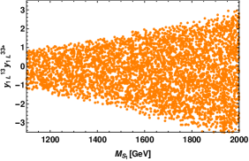
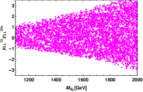
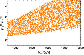
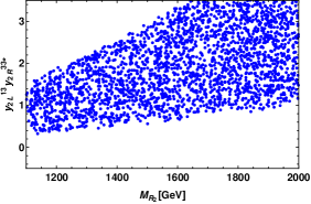
Figure 1: Constraints on scalar leptoquark masses and couplings (real) associated with $b\to u\tau\bar{\nu}_{\tau}$ decay processes.

For the case of $b\to c\tau\bar{\nu}_{\tau}$, the constraints on $y_{1L}^{33}y_{1L}^{23^{*}}~{}(y_{3L}^{33}y_{3L}^{23^{*}})$ product of couplings of the $S_{1}(S_{3})$ leptoquarks and their corresponding masses are depicted in the top-left (top-right) panel of Fig. 2 . The bottom-left panel of Fig. 2 represents the allowed region of $y_{1L}^{33}y_{1R}^{23^{*}}$ couplings and masses of $S_{1}$ leptoquarks and the corresponding plot for $R_{2}$ leptoquark is shown in the bottom-right panel.

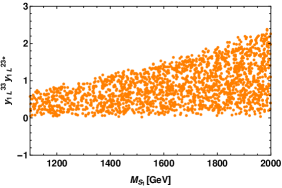
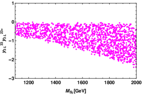
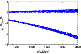
Figure 2: Constraints on scalar leptoquark masses and couplings (real) associated with $b\to c\tau\bar{\nu}_{\tau}$ decay processes.

In Table 1 , we give the allowed ranges of leptoquark masses and real couplings obtained by imposing the extrema conditions.

Table 1: Minimum and maximum values of the leptoquark couplings (real) and masses.

Decay processes	Leptoquarks	Couplings	Real part	Mass of leptoquark
			(Min, Max)	(Min, Max)
$b\to u\tau\bar{\nu}_{\tau}$	$S_{1}$	$y_{1L}^{33}y_{1L}^{13^{*}}$	$(-3.5,3.0)$	$(1100,2000)$
		$y_{1L}^{33}y_{1R}^{13^{*}}$	$(0.3,3.5)$	$(1100,2000)$
	$S_{3}$	$y_{3L}^{33}y_{3L}^{13^{*}}$	$(-3.0,3.5)$	$(1100,2000)$
	$R_{2}$	$y_{2L}^{13}y_{2R}^{33^{*}}$	$(0.3,3.5)$	$(1100,2000)$
$b\to c\tau\bar{\nu}_{\tau}$	$S_{1}$	$y_{1L}^{33}y_{1L}^{23^{*}}$	$(0.0,2.2)$	$(1100,2000)$
		$y_{1L}^{33}y_{1R}^{23^{*}}$	$(-0.32,0.0)$	$(1100,2000)$
	$S_{3}$	$y_{3L}^{33}y_{3L}^{23^{*}}$	$(-2.2,0.0)$	$(1100,2000)$
	$R_{2}$	$y_{2L}^{23}y_{2R}^{33^{*}}$	$(0.0,0.32)$	$(1100,2000)$

III.1.2 Complex couplings

Considering the leptoquarks couplings as complex, the constraint on the real and imaginary parts of $y_{1L}^{33}y_{1L}^{13^{*}}~{}(y_{1L}^{33}y_{1R}^{13^{*}})$ couplings of $S_{1}$ leptoquark is depicted in the top-left (bottom-left) panel of Fig. 3 . The allowed space of $y_{3L}^{33}y_{3L}^{13^{*}}$ and $y_{2L}^{13}y_{2L}^{33^{*}}$ couplings obtained from the Br($B_{u}\to\tau\nu_{l}$), Br($B\to\pi\tau\nu_{l}$) and $R_{\pi}^{l}$ experimental data are shown in the top-right and bottom-right panels of Fig. 3 .

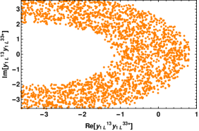
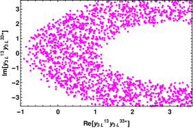
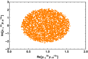
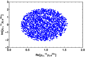
Figure 3: Constraints on real and imaginary part of the leptoquark couplings associated with $b\to u\tau\bar{\nu}_{\tau}$ decay processes.

Imposing the experimental limit on Br($B_{c}\to\tau\nu_{\tau}$), $R_{D^{(*)}}$ and $R_{J/\psi}$ observables, the constraints on real and imaginary parts of the vectorial type couplings of $S_{1}~{}(S_{3})$ leptoquark are presented in the top-left (top-right) panel of Fig. 4 . The corresponding constrained plots for the scalar couplings of $S_{1}$ and $R_{2}$ leptoquarks are given in the bottom-left and bottom-right panel of this figure.

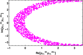
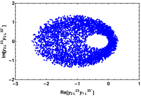
Figure 4: Constraints on real and imaginary part of the leptoquark couplings associated with $b\to c\tau\bar{\nu}_{\tau}$ decay processes.

The obtained allowed new parameter space is presented in Table 2 .

Table 2: Minimum and maximum values of the real and imaginary parts of the leptoquarks couplings.

Decay processes	Leptoquarks	Couplings	Real part	Imaginary part
			(Min, Max)	(Min, Max)
$b\to u\tau\bar{\nu}_{\tau}$	$S_{1}$	$y_{1L}^{33}y_{1L}^{13^{*}}$	$(-1.4,0.6)$	$(-3.5,3.5)$
		$y_{1L}^{33}y_{1R}^{13^{*}}$	$(0.3,1.6)$	$(-2.0,2.0)$
	$S_{3}$	$y_{3L}^{33}y_{3L}^{13^{*}}$	$(-0.6,1.4)$	$(-3.5,3.5)$
	$R_{2}$	$y_{2L}^{13}y_{2R}^{33^{*}}$	$(0.3,1.6)$	$(-2.0,2.0)$
$b\to c\tau\bar{\nu}_{\tau}$	$S_{1}$	$y_{1L}^{33}y_{1L}^{23^{*}}$	$(-0.2,0.6)$	$(-3.5,3.5)$
		$y_{1L}^{33}y_{1R}^{23^{*}}$	$(-0.35,0.1)$	$(-1.4,1.4)$
	$S_{3}$	$y_{3L}^{33}y_{3L}^{23^{*}}$	$(-0.6,0.2)$	$(-3.5,3.5)$
	$R_{2}$	$y_{2L}^{23}y_{2R}^{33^{*}}$	$(-2.4,-0.6)$	$(-1.4,1.4)$

IV Numerical analysis

In this section, we perform the numerical analysis of the branching ratios and physical observables of $B_{s}\to(K^{(*)},D_{s}^{(*)})\tau\bar{\nu}_{\tau}$ processes. For numerical estimation, we use the particle masses, life time of $B_{s}$ meson and the CKM matrix elements from Patrignani et al. (2016) . The predictions for the various observables require sufficient knowledge of the associated hadronic form factors. For $\bar{B}_{s}\to K^{+}l^{-}\bar{\nu}_{l}$ decay processes, we consider the perturbative QCD (PQCD) calculation Wang and Xiao (2012); Mei ner and Wang (2014) based on the $k_{T}$ factorization Keum et al. (2001a, b); Lu et al. (2001); Lu and Yang (2002) at next-to-leading order (NLO) in $\alpha_{s}$ Li et al. (2012), which gives

$$F_{1}^{B_{s}\to K}(q^{2}) = {F_{1}^{B_{s}\to K}(0)}\left(\frac{1}{(1-q^{2}/M_{B_{s}}^{2})}+\frac{a_{1}q^{2}/M_{B_{s}}^{2}}{(1-q^{2}/M_{B_{s}}^{2})(1-b_{1}q^{2}/M_{B_{s}}^{2})}\right),$$

$$F_{0}^{B_{s}\to K}(q^{2}) = \frac{F_{0}^{B_{s}\to K}(0)}{(1-a_{0}q^{2}/M_{B_{s}}^{2}+b_{0}q^{4}/M_{B_{s}}^{4})}~{}.$$ (27)

The values of the parameters $a_{0,1}$, $b_{0,1}$ and $F_{0,1}^{B_{s}\to K}$ can be found in the Ref. Wang and Xiao (2012). The $q^{2}$ dependence of the form factors $V,A_{0,1,2},T_{1,2,3}$ associated with $B_{s}\to K^{*}\tau\bar{\nu}_{\tau}$ decay modes can be parametrized as Ball and Zwicky (2005)

$$f_{1}^{B_{s}\to K^{*}}\left(q^{2}\right) = \frac{r_{1}}{1-q^{2}/m^{2}_{R}}+\frac{r_{2}}{1-q^{2}/m^{2}_{fit}}\;,~{}~{}~{}~{}~{}~{}~{}f_{1}=V,A_{0},T_{1},$$

$$f_{2}^{B_{s}\to K^{*}}\left(q^{2}\right) = \frac{r_{2}}{1-q^{2}/m^{2}_{fit}}\;,\hskip 99.58464ptf_{2}=A_{1},T_{2},$$

$$f_{3}^{B_{s}\to K^{*}}\left(q^{2}\right) = \frac{r_{1}}{1-q^{2}/m^{2}_{fit}}+\frac{r_{2}}{\left(1-q^{2}/m^{2}_{fit}\right)^{2}},~{}~{}~{}f_{3}=A_{2},\tilde{T_{3}}\;,$$ (28)

where $T_{3}$ is related to $\tilde{T}_{3}$ and the values of the parameters involved in the calculation of form factors are taken from Ref. Ball and Zwicky (2005). The $B_{s}\to D_{s}^{(*)}\tau\bar{\nu}_{\tau}$ form factors, computed by using the PQCD approach Fan et al. (2014) are used in this analysis, which can be parametrized as

$$F^{B_{s}\to D_{s}^{(*)}}(q^{2}) = \frac{F^{B_{s}\to D_{s}^{(*)}}(0)}{(1-aq^{2}/M_{B_{s}}^{2}+bq^{4}/M_{B_{s}}^{4})}\,,$$ (29)

where $F^{B_{s}\to D_{s}^{(*)}}$ stand for the form factors $F_{0,+},V,A_{0,1,2}$. The fitting values of the $a$ and $b$ parameters can be found in Fan et al. (2014). Since there is no PQCD results on the form factors associated with tensor operator, we show our results for $B_{s}\to D_{s}^{(*)}l\bar{\nu}_{l}$ process with vanishing tensor form factors.

Now the stage is ready with detailed expressions of physical observables, required input parameters and the constrained new Wilson coefficients for complete numerical anaysis. Using these input values, the predicted branching ratios $B_{s}\to(K^{(*)},D_{s}^{(*)})\mu\bar{\nu}_{l}$ processes in the SM are given by

$${\rm Br}(B_{s}\to K\mu\bar{\nu}_{\mu})^{\rm SM}=(1.044\pm 0.084)\times 10^{-4},$$ (30)

$${\rm Br}(B_{s}\to K^{*}\mu\bar{\nu}_{\mu})^{\rm SM}=(3.43\pm 0.275)\times 10^{-4},$$ (31)

$${\rm Br}(B_{s}\to D_{s}\mu\bar{\nu}_{\mu})^{\rm SM}=(2.17\pm 0.174)\times 10^{-2},$$ (32)

$${\rm Br}(B_{s}\to D_{s}^{*}\mu\bar{\nu}_{\mu})^{\rm SM}=(4.82\pm 0.386)\times 10^{-2}.$$ (33)

In the following subsection, we discuss the impact of individual scalar leptoquarks on the branchings ratios and the optimized physical observables of semileptonic $B_{s}$ decay modes.

IV.1 $S_{1}$ scalar leptoquark

This subsection is dedicated to the analysis of $B_{s}\to(K^{(*)},D_{s}^{(*)})\tau\bar{\nu}_{\tau}$ physical observables by using the singlet $S_{1}(\bar{3},1,1/3)$ scalar LQ. This LQ will contribute additional $V_{L},~{}S_{R}$ and $T_{L}$ coefficients to the SM. The constraint on the the couplings (real and complex) and masses associated with this leptoquark are obtained by using the Br($B_{u,c}\to\tau\nu_{\tau}$), Br($B\to\pi\tau\tau$), $R_{\pi}^{l}$, $R_{D^{(*)}}$ and $R_{J/\psi}$ observables, as discussed in section III. Using the allowed space of real and complex couplings and the leptoquark mass from Table 1 and 2 , we show the variation of the branching ratios of $B_{s}\to K\tau\bar{\nu}_{\tau}$ (top-left panel), $B_{s}\to K^{*}\tau\bar{\nu}_{\tau}$ (top-right panel), $B_{s}\to D_{s}\tau\bar{\nu}_{\tau}$ (bottom-left panel) and $B_{s}\to D_{s}^{*}\tau\bar{\nu}_{\tau}$ (bottom-right panel) processes with respect to $q^{2}$ in Fig. 5 . Here the cyan bands represent the contributions coming due to the $S_{1}$ SLQ exchange, where coupling is complex. The orange bands are due to the SLQ contributions with real couplings. The red dashed lines present the central values of standard model and their corresponding theoretical uncertainties, arising due to the uncertainties associated with hardonic form factors and CKM matrix elements, are shown in gray color. We found that the branching ratios of all these processes deviate significantly from their corresponding SM predictions due to the additional contribution from the complex couling of $S_{1}$ scalar leptoquark. Though the region of real coupling case provide deviation from the SM results, these are comparatively less than the case of complex coupling. The numerical values of the braching ratios of these decay modes for the SM and for all the cases of $S_{1}$ leptoquark couplings are presented in the Table 3 .

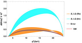
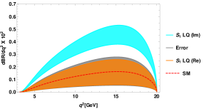
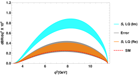
Figure 5: The variation of branching ratios of $\bar{B}_{s}\to K^{+}l^{-}\bar{\nu}_{\tau}$ (top-left panel), $\bar{B}_{s}\to K^{*+}l^{-}\bar{\nu}_{\tau}$ (top-right panel), $\bar{B}_{s}\to D_{s}^{+}l^{-}\bar{\nu}_{\tau}$ (bottom-left panel) and $\bar{B}_{s}\to D_{s}^{*+}l^{-}\bar{\nu}_{\tau}$ (bottom-right panel) processes with respect to $q^{2}$ in the $S_{1}$ scalar leptoquark model. Here cyan bands are due to the contribution from $S_{1}$ leptoquark with coupling as complex. The orange bands stand for the allowed regions of real leptoquark coulings. The red dashed lines represent the standard model contributions with their corresponding theoretical uncertainties are shown in gray bands.

Beyond the branching ratios, another interesting observable is the zero crossing of forward-backward asymmetry. The $q^{2}$ variation of the forward-backward asymmetries of $B_{s}\to K\tau\bar{\nu}_{\tau}$ (top-left panel), $B_{s}\to K^{*}\tau\bar{\nu}_{\tau}$ (top-right panel), $B_{s}\to D_{s}\tau\bar{\nu}_{\tau}$ (bottom-left panel) and $B_{s}\to D_{s}^{*}\tau\bar{\nu}_{\tau}$ (bottom-right panel) decay modes in the $S_{1}$ scalar leptoquark model are presented in Fig. 6 . The case of real leptoquark coupling provides significant deviation in the forward-backward asymmetries of $B_{s}\to K^{(*)}\tau\bar{\nu}_{\tau}$ processes from their SM values, where as the case of complex leptoquark coupling provides comparatively less deviation. The constrained couplings(real and complex) have almost negligible impact on the forward-backward asymmetries linked to the $B_{s}\to D_{s}^{(*)}\tau\bar{\nu}_{\tau}$ channels. The numerical values of the forward-backward asymmetry are given in Table 3 .

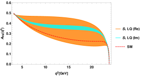
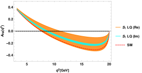
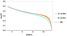
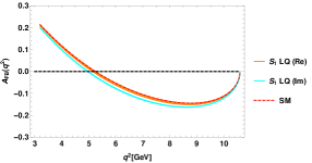
Figure 6: The variation of forward-backward asymmetry of $\bar{B}_{s}\to K^{+}\tau^{-}\bar{\nu}_{\tau}$ (top-left panel), $\bar{B}_{s}\to K^{*+}\tau^{-}\bar{\nu}_{\tau}$ (top-right panel), $\bar{B}_{s}\to D_{s}^{+}\tau^{-}\bar{\nu}_{\tau}$ (bottom-left panel) and $\bar{B}_{s}\to D_{s}^{*+}\tau^{-}\bar{\nu}_{\tau}$ (bottom-right panel) processes with respect to $q^{2}$ in the $S_{1}$ scalar leptoquark model.

Fig. 7  depicts the variation of the lepton non-universality parameters $R_{K}^{\tau\mu}$ (top-left panel), $R_{K^{*}}^{\tau\mu}$ (top-right panel), $R_{D_{s}}^{\tau\mu}$ (bottom-left panel) and $R_{D_{s}^{*}}^{\tau\mu}$ (bottom-right panel) with respect to $q^{2}$. It is found that, the allowed real coupling region has more effect on $R_{K^{(*)}}^{\tau\mu}$ LNU parameters and the complex leptoquark couplings affect the $R_{D_{s}^{(*)}}^{\tau\mu}$ parameters. In Table 3, the numerical values of the lepton non-universality parameters are shown.

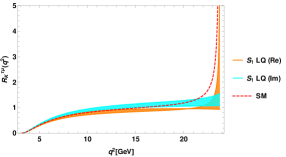
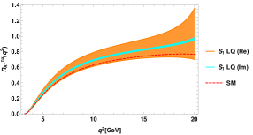
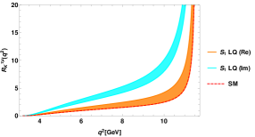
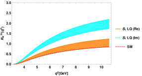
Figure 7: The variation of lepton non-universality prameters of $\bar{B}_{s}\to K^{+}\tau^{-}\bar{\nu}_{\tau}$ (top-left panel), $\bar{B}_{s}\to K^{*+}\tau^{-}\bar{\nu}_{\tau}$ (top-right panel), $\bar{B}_{s}\to D_{s}^{+}\tau^{-}\bar{\nu}_{\tau}$ (bottom-left panel) and $\bar{B}_{s}\to D_{s}^{*+}\tau^{-}\bar{\nu}_{\tau}$ (bottom-right panel) processes with respect to $q^{2}$ in the $S_{1}$ scalar leptoquark model.

The plots in the Fig. 8 , show the effect of new parameter space on the $\tau$-polarization asymmetries of $B_{s}\to K\tau\bar{\nu}_{\tau}$ (top-left panel), $B_{s}\to K^{*}\tau\bar{\nu}_{\tau}$ (top-right panel), $B_{s}\to D_{s}\tau\bar{\nu}_{\tau}$ (bottom-left panel) and $B_{s}\to D_{s}^{*}\tau\bar{\nu}_{\tau}$ (bottom-right panel) processes. We observe profound deviation in the polarization asymmety of $B_{s}\to K^{(*)}\tau\bar{\nu}_{\tau}$ decay modes due to the $S_{1}$ SLQ contribution with the coupling as real. The contribution from the complex LQ couplings also deviate the $\tau$-polarization asymmetry parameters from their SM predictions. The complex coulings region affect the $\tau$-polarization asymmetry $B_{s}\to D_{s}\tau\bar{\nu}_{l}$ significantly. There is no much impact of new physics on the $B_{s}\to D_{s}^{*}\tau\bar{\nu}_{l}$ decay proess.

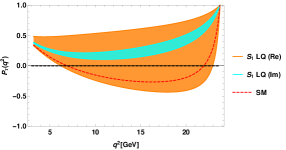
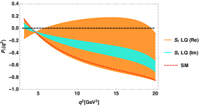
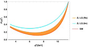
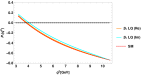
Figure 8: The variation of lepton polarization asymmetry parameters of $\bar{B}_{s}\to K^{+}\tau^{-}\bar{\nu}_{\tau}$ (top-left panel), $\bar{B}_{s}\to K^{*+}\tau^{-}\bar{\nu}_{\tau}$ (top-right panel), $\bar{B}_{s}\to D_{s}^{+}\tau^{-}\bar{\nu}_{\tau}$ (bottom-left panel) and $\bar{B}_{s}\to D_{s}^{*+}\tau^{-}\bar{\nu}_{\tau}$ (bottom-right panel) processes with respect to $q^{2}$ in the $S_{1}$ scalar leptoquark model.

The $K^{*}$ $(D_{s}^{*})$ polarization asymmetry plot for the $B_{s}\to K^{*}\tau\bar{\nu}_{\tau}$ $(B_{s}\to D_{s}^{*}\tau\bar{\nu}_{\tau})$ mode is presented in the left panel (right panel) of Fig. 9 . The predicted numerical values of all these observables are given in 3 .

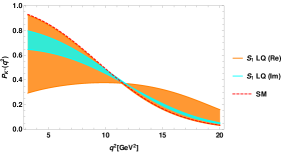
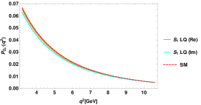
Figure 9: The variation of hardon polarization asymmetry parameters of $\bar{B}_{s}\to K^{*+}\tau^{-}\bar{\nu}_{\tau}$ (left panel) and $\bar{B}_{s}\to D_{s}^{*+}\tau^{-}\bar{\nu}_{\tau}$ (right panel) processes with respect to $q^{2}$ in the $S_{1}$ scalar leptoquark model.

Table 3: The predicted values of the branching ratios and other physical observables of $B_{s}\to(K^{(*)},D_{s}^{(*)})\tau\bar{\nu}_{\tau}$ proesses in the SM and in the $S_{1}$ scalar leptoquark model. Here RC represents the real coupling region and CC stands for complex coupling.

	Observables	Values for SM	Values for RC	Values for CC
$B_{s}$	Br	$(6.65\pm 0.532)\times 10^{-5}$	$(5.35-9.36)\times 10^{-5}$	$(2.43-3.056)\times 10^{-4}$
$\downarrow$	$\langle A_{FB}^{\tau}\rangle$	$0.278\pm 0.022$	$0.25-0.42$	$0.348-0.369$
$K$	$\langle P_{\tau}\rangle$	$-0.1567\pm 0.013$	$-0.283\to 0.657$	$0.22-0.368$
	$\langle R_{K}^{\tau\mu}\rangle$	$0.6365$	$0.512-0.896$	$2.33-2.93$
$B_{s}$	Br	$(1.85\pm 0.148)\times 10^{-4}$	$(0.68-2.95)\times 10^{-4}$	$(4.38-6.09)\times 10^{-4}$
$\downarrow$	$\langle A_{FB}^{\tau}\rangle$	$-0.182\pm 0.015$	$-0.196\to-0.015$	$-0.131\to-0.111$
$K^{*}$	$\langle P_{\tau}\rangle$	$-0.585\pm 0.045$	$-0.61\to 0.122$	$-0.405\to-0.27$
	$\langle P_{K^{*}}\rangle$	$0.191\pm 0.015$	$0.185-0.313$	$0.213-0.225$
	$\langle R_{K^{*}}^{\tau\mu}\rangle$	$0.54$	$0.198-0.858$	$1.275-1.772$
$B_{s}$	Br	$(1.39\pm 0.111)\times 10^{-2}$	$(1.39-2.26)\times 10^{-2}$	$(3.93-4.67)\times 10^{-2}$
$\downarrow$	$\langle A_{FB}^{\tau}\rangle$	$0.358\pm 0.029$	$0.353-0.358$	$0.329-0.333$
$D_{s}$	$\langle P_{\tau}\rangle$	$0.2\pm 0.016$	$0.2-0.284$	$0.418-0.422$
	$\langle R_{D_{s}}^{\tau\mu}\rangle$	$0.6415$	$0.6415-1.04$	$1.808-2.2867$
$B_{s}$	Br	$(2.23\pm 0.178)\times 10^{-2}$	$(2.23-3.215)\times 10^{-2}$	$(4.5-5.62)\times 10^{-2}$
$\downarrow$	$\langle A_{FB}^{\tau}\rangle$	$-0.0996\pm 0.008$	$-0.107\to-0.0996$	$-0.12\to-0.118$
$D_{s}^{*}$	$\langle P_{\tau}\rangle$	$-0.514\to 0.0411$	$-0.514\to-0.5$	$-0.4766\to-0.4746$
	$\langle P_{D_{s}^{*}}\rangle$	$0.0113\to 0.0009$	$0.011-0.0113$	$0.0107-0.0108$
	$\langle R_{D_{s}^{*}}^{\tau\mu}\rangle$	$0.463$	$0.463-0.6673$	$0.9313-1.167$

IV.2 $S_{3}$ scalar leptoquark

The triplet $S_{3}(\bar{3},1,1/3)$ scalar leptoquark contributes only additional $V_{L}$ Wilson coefficient to the SM. The allowed new parameter space obtained from the available experimental data on relevant observables, for both real and complex coupling cases are already provided in section III. Now using the constrained parameters, the branching ratios of $B_{s}\to K\tau\bar{\nu}_{\tau}$ (top-left panel), $B_{s}\to K^{*}\tau\bar{\nu}_{\tau}$ (top-right panel), $B_{s}\to D_{s}\tau\bar{\nu}_{\tau}$ (bottom-left panel) and $B_{s}\to D_{s}^{*}\tau\bar{\nu}_{\tau}$ (bottom-right panel) decay modes with $q^{2}$ in the $S_{3}$ scalar letoquark model are shown in Fig. 10 . Here the cyan color bands are arising due to the constrained complex coupligs and the magneta bands represent the new physics contributions to the branching ratios predicted from the allowed region of $S_{3}$ leptoquark with real couplings. We found that, the branching ratios of all these decay modes deviate significantly from SM for the case of both complex and real couplings. The predicted branching ratios for all the cases of new couplings are given in Table 4 .

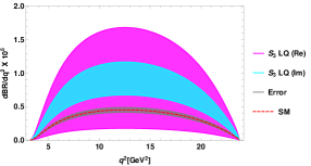
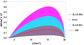
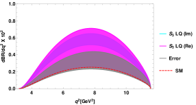
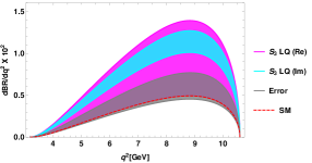
Figure 10: The variation of branching ratios of $\bar{B}_{s}\to K^{+}\tau^{-}\bar{\nu}_{\tau}$ (top-left panel), $\bar{B}_{s}\to K^{*+}\tau^{-}\bar{\nu}_{\tau}$ (top-right panel), $\bar{B}_{s}\to D_{s}^{+}\tau^{-}\bar{\nu}_{\tau}$ (bottom-left panel) and $\bar{B}_{s}\to D_{s}^{*+}\tau^{-}\bar{\nu}_{\tau}$ (bottom-right panel) processes with respect to $q^{2}$ in the $S_{3}$ scalar leptoquark model. Here cyan bands represent the case of complex $S_{3}$ leptoquark coupling and the magenta bands stand for real coupling.

In Fig. 11 , the lepton non-universality parameters for $B_{s}\to D_{s}\tau\bar{\nu}_{\tau}$ and $B_{s}\to D_{s}^{*}\tau\bar{\nu}_{\tau}$ are shown in the left and right panels, respectively. For this observables, the complex leptoquark coupling are found to be more effective in comparison to the case of real coupling. However, the impact of $S_{3}$ leptoquark on the $R_{K^{(*)}}^{\tau\mu}$ parameter of $B_{s}\to K^{(*)}\tau\bar{\nu}_{\tau}$ processes are found to be negligible. The numerical values of the LNU parameters of all these decay modes are presented in Table 4 . We don’t find any deviation in the forward-backward asymmetry, lepton and hadron polarization asymmetry parameters of semileptonic $B_{s}$ decay processes due to the additional NP contributions from $S_{3}$ scalar LQ.

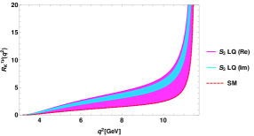
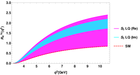
Figure 11: The variation of lepton nonuniversality prameters of $\bar{B}_{s}\to D_{s}^{+}\tau^{-}\bar{\nu}_{\tau}$ (left panel) and $\bar{B}_{s}\to D_{s}^{*+}\tau^{-}\bar{\nu}_{\tau}$ (right panel) processes with respect to $q^{2}$ in the $S_{3}$ scalar leptoquark model.

Table 4: The predicted values of the branching ratios and other physical observables of $B_{s}\to(K^{(*)},D_{s}^{(*)}\tau\bar{\nu}_{\tau})$ proesses in the SM and in the $S_{3}$ scalar leptoquark model. Here RC represents the real coupling and CC stands for complex coupling.

Observables	Values for RC	Values for CC
Br($B_{s}\to K\tau\bar{\nu}_{l}$)	$(0.26-2.47)\times 10^{-4}$	$(0.993-1.71)\times 10^{-4}$
Br($B_{s}\to K^{*}\tau\bar{\nu}_{l}$)	$(0.73-6.9)\times 10^{-4}$	$(2.77-4.78)\times 10^{-4}$
Br($B_{s}\to D_{s}\tau\bar{\nu}_{l}$)	$(2.26-3.94)\times 10^{-2}$	$(2.86-3.59)\times 10^{-2}$
$\langle R_{D_{s}}^{\tau\mu}\rangle$	$0.6415-1.812$	$1.317-1.654$
Br($B_{s}\to D_{s}^{*}\tau\bar{\nu}_{l}$)	$(4.82-6.3)\times 10^{-2}$	$(4.6-5.74)\times 10^{-2}$
$\langle R_{D_{s}^{*}}^{\tau\mu}\rangle$	$0.463-1.307$	$0.95-1.193$

IV.3 $R_{2}$ scalar leptoquark

After discussing the impact of $S_{1,3}$ scalar leptoquarks on the flavor observables of $B_{s}$ decay modes mediated by the $b\to(u,c)\tau\bar{\nu}_{\tau}$ transitions, we now proceed to check the same physical observables in the $R_{2}(3,2,7/6)$ SLQ model. $R_{2}$ LQ is doublet under $SU(2)$ and contributes only scalar and tensor type couplings to the SM. The variation of branching ratios of $B_{s}\to K\tau\bar{\nu}_{\tau}$ (top-left panel), $B_{s}\to K^{*}\tau\bar{\nu}_{\tau}$ (top-right panel), $B_{s}\to D_{s}\tau\bar{\nu}_{\tau}$ (bottom-left panel) and $B_{s}\to D_{s}^{*}\tau\bar{\nu}_{\tau}$ (bottom-right panel) processes with $q^{2}$, obtained by using the allowed parameter space of $R_{2}$ leptoquark (1, 2) are given in Fig. 12 . Here the blue bands are due to the constrained real couplings and the cyan bands are for the complex $R_{2}$ leptoquark couplings. We observe that, the branching ratios of $B_{s}\to(K,D_{s})$ modes show profound deviatation from their corresponding SM results due to the additional complex coupling contributions. The real coupling has more effect on Br$(B_{s}\to K^{*}\tau\bar{\nu}_{\tau})$ in comarison to the case of complex parmeters. Where as there is no deviation in the branching ratio of $B_{s}\to D_{s}^{*}\tau\bar{\nu}_{\tau}$ due to the presence of $R_{2}$ leptoquark. The predicted values of branching ratios for both real and complex couplings cases are presented in Table 5 .

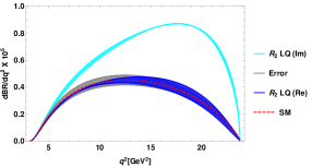
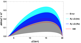
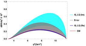
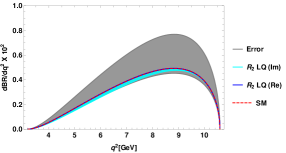
Figure 12: The variation of branching ratios of $\bar{B}_{s}\to K^{+}\tau^{-}\bar{\nu}_{\tau}$ (top-left panel), $\bar{B}_{s}\to K^{*+}\tau^{-}\bar{\nu}_{\tau}$ (top-right panel), $\bar{B}_{s}\to D_{s}^{+}\tau^{-}\bar{\nu}_{\tau}$ (bottom-left panel) and $\bar{B}_{s}\to D_{s}^{*+}\tau^{-}\bar{\nu}_{\tau}$ (bottom-right panel) processes with respect to $q^{2}$ in the $R_{2}$ scalar leptoquark model. Here cyan bands represent the case of complex $S_{3}$ leptoquark coupling and the blue bands stand for real coupling.

Fig. 13 describes the variation of the forward-backward asymmetry of $B_{s}\to K\tau\bar{\nu}_{\tau}$ (top-left panel), $B_{s}\to K^{*}\tau\bar{\nu}_{\tau}$ (top-right panel), $B_{s}\to D_{s}\tau\bar{\nu}_{\tau}$ (bottom-left panel) and $B_{s}\to D_{s}^{*}\tau\bar{\nu}_{\tau}$ (bottom-right panel) with respect to $q^{2}$. The $A_{FB}$ of $B_{s}\to K^{(*)}$ deviate significantly due to additional $R_{2}$ leptoquark whereas very minor effect of new parameters are observed for $B_{s}\to D_{s}^{(*)}$ modes. The numerical values of forward-backward asymmetries for both real and complex couplings cases are given in Table 5 .

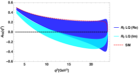
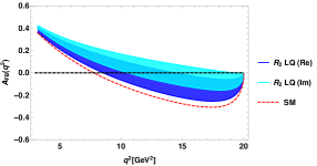
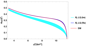
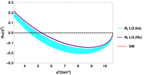
Figure 13: The variation of forward-backward asymmetry of $\bar{B}_{s}\to K^{+}\tau^{-}\bar{\nu}_{\tau}$ (top-left panel), $\bar{B}_{s}\to K^{*+}\tau^{-}\bar{\nu}_{\tau}$ (top-right panel), $\bar{B}_{s}\to D_{s}^{+}\tau^{-}\bar{\nu}_{\tau}$ (bottom-left panel) and $\bar{B}_{s}\to D_{s}^{*+}\tau^{-}\bar{\nu}_{\tau}$ (bottom-right panel) processes with respect to $q^{2}$ in the $R_{2}$ scalar leptoquark model.

In Fig. 14 , we depict the variation of $R_{K}^{\tau\mu}$ (top-left panel), $R_{K^{*}}^{\tau\mu}$ (top-right panel), $R_{D_{s}}^{\tau\mu}$ (bottom-left panel) and $R_{D_{s}^{*}}^{\tau\mu}$ (bottom-right panel) LNU parameters. The impact of $R_{2}$ leptoquark on the $R_{D_{s}^{(*)}}^{\tau\mu}$ LNU parameters are found to be negligible. Table 5  contains the numerical values of all the LNU parameters.

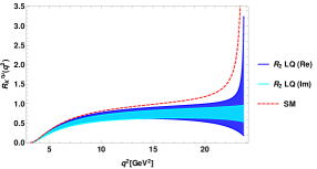
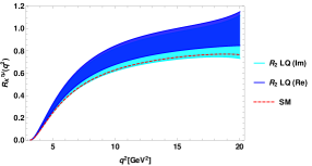
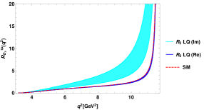
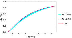
Figure 14: The variation of lepton nonuniversality prameters of $\bar{B}_{s}\to K^{+}\tau^{-}\bar{\nu}_{\tau}$ (top-left panel), $\bar{B}_{s}\to K^{*+}\tau^{-}\bar{\nu}_{\tau}$ (top-right panel), $\bar{B}_{s}\to D_{s}^{+}\tau^{-}\bar{\nu}_{\tau}$ (bottom-left panel) and $\bar{B}_{s}\to D_{s}^{*+}\tau^{-}\bar{\nu}_{\tau}$ (bottom-right panel) processes with respect to $q^{2}$ in the $R_{2}$ scalar leptoquark model.

The $\tau$ polarization asymmetries of all these decay modes are given in Fig. 15 . The left and right panel of Fig. 16 presents the $K^{*}$ and $D_{s}^{*}$ polarization asymmetry parameters respectively. In Table 5 , the predicted numerical values of lepton and hardon polarization asymmetries are listed.

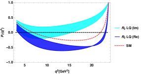
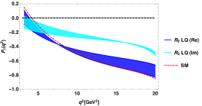
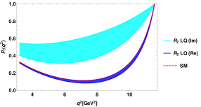
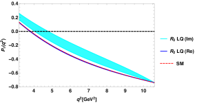
Figure 15: The variation of lepton polarization asymmetry parameters of $\bar{B}_{s}\to K^{+}\tau^{-}\bar{\nu}_{\tau}$ (top-left panel), $\bar{B}_{s}\to K^{*+}\tau^{-}\bar{\nu}_{\tau}$ (top-right panel), $\bar{B}_{s}\to D_{s}^{+}\tau^{-}\bar{\nu}_{\tau}$ (bottom-left panel) and $\bar{B}_{s}\to D_{s}^{*+}\tau^{-}\bar{\nu}_{\tau}$ (bottom-right panel) processes with respect to $q^{2}$ in the $R_{2}$ scalar leptoquark model.

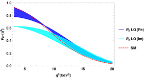
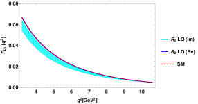
Figure 16: The variation of hardon polarization asymmetry parameters of $\bar{B}_{s}\to K^{*+}\tau^{-}\bar{\nu}_{\tau}$ (left panel) and $\bar{B}_{s}\to D_{s}^{*+}\tau^{-}\bar{\nu}_{\tau}$ (right panel) processes with respect to $q^{2}$ in the $R_{2}$ scalar leptoquark model.

Table 5: The predicted values of the branching ratios and other physical observables of $B_{s}\to(K^{(*)},D_{s}^{(*)}\tau\bar{\nu}_{\tau})$ proesses in the SM and in the $R_{2}$ scalar leptoquark model. Here RC represents the real coupling region and CC stands for complex coupling.

	Observables	Values for RC	Values for CC
$B_{s}$	Br	$(6.2-7.0)\times 10^{-5}$	$(1.25-1.278)\times 10^{-4}$
$\downarrow$	$\langle A_{FB}\rangle$	$-0.029\to 0.27$	$-0.204\to-0.029$
$K$	$\langle P_{\tau}\rangle$	$-0.516\to-0.322$	$0.054-0.347$
	$\langle R_{K}^{\tau\mu}\rangle$	$0.593-0.671$	$1.198-1.224$
$B_{s}$	Br	$(2.0-3.15)\times 10^{-4}$	$(2.47-3.93)\times 10^{-4}$
$\downarrow$	$\langle A_{FB}^{\tau}\rangle$	$-0.134\to 0.047$	$-0.041\to 0.1143$
$K^{*}$	$\langle P_{\tau}\rangle$	$-0.6\to-0.5$	$-0.31\to-0.278$
	$\langle P_{K^{*}}\rangle$	$0.21-0.281$	$0.19-0.285$
	$\langle R_{K^{*}}^{\tau\mu}\rangle$	$0.591-0.917$	$0.719-1.146$
$B_{s}$	Br	$(1.34-1.39)\times 10^{-2}$	$(2.0-3.74)\times 10^{-2}$
$\downarrow$	$\langle A_{FB}^{\tau}\rangle$	$0.358$	$0.255-0.3$
$D_{s}$	$\langle P_{\tau}\rangle$	$0.1674-0.2$	$0.45-0.7$
	$\langle R_{D_{s}}^{\tau\mu}\rangle$	$0.16-0.6415$	$0.934-1.72$
$B_{s}$	Br	$(2.23-2.24)\times 10^{-2}$	$(2.1-2.2)\times 10^{-2}$
$\downarrow$	$\langle A_{FB}^{\tau}\rangle$	$-0.0996\to-0.097$	$-0.164\to-0.115$
$D_{s}^{*}$	$\langle P_{\tau}\rangle$	$-0.519\to-0.514$	$-0.475\to-0.374$
	$\langle P_{D_{s}^{*}}\rangle$	$0.0113-0.0114$	$0.0099-0.011$
	$\langle R_{D_{s}^{*}}^{\tau\mu}\rangle$	$0.43-0.464$	$0.438-0.457$

V Summary and Conclusion

To summarize the article, we have studied the rare semileptonic decay processes of $B_{s}$ meson i.e, $B_{s}\to(K^{(*)},D_{s}^{(*)})\tau\bar{\nu}_{\tau}$ mediated by the $b\to(u,c)\tau\bar{\nu}_{l}$ quark level transitions in the context of scalar leptoquark model. Our main motivation was to see how the singlet $S_{1}(\bar{3},1,1/3)$, doublet $R_{2}(\bar{3},2,7/6)$ and the triplet $S_{3}(\bar{3},3,1/3)$ leptoquarks affect the braching ratios and other physical observables like forward-backward asymmetry, lepton non-universality parameter, lepton and hardon polarization asymmetry associated with these decay modes. The $S_{1}$ leptoquark contributes additional vector, scalar and tensor couplings to the standard model, where as the $S_{3}$ leptoquark contributes only $V_{L}$ coefficient and the $R_{2}$ leptoquark provides scalar and tensor couplings contributions. We have considered that the new physics contributes only to the tau lepton and the contribution to the first and second generation leptons are assumed to be SM like. We then considered two valid cases of leptoquark couplings, real and complex. We have used the experimental limit on the branching ratios of $B_{u}\to\tau\nu_{\tau}$ and $B\to\pi\tau\tau$ and the $R_{\pi}^{l}$ parameters to constrain the new leptoquark couplings related to the $b\to u\tau\bar{\nu}_{\tau}$ transition. For the case of $b\to c\tau\bar{\nu}_{\tau}$ processes, we have computed the allowed parameter space by using the branching ratio of $B_{c}\to\tau\nu_{\tau}$ obtained by using the life time of $B_{c}$ meson and the $R_{D^{(*)}},~{}R_{J/\psi}$ parameters. Using the allowed parameter space, we have estimated the branchng ratios and other observables of $B_{s}\to(K^{(*)},D_{s}^{(*)})\tau\bar{\nu}_{\tau}$ modes.

We have observed that the branching ratios of all these decay processes deviate significantly from their corresponding SM results due to the new contributions from the complex couplings of $S_{1}$ leptoquark. However the region of the constrained real couplings show negligible effect on the branching ratios of these decay modes. The impact of $S_{1}$ leptoquark on the forward-backward asymmetry of $B_{s}\to K^{(*)}\tau\bar{\nu}_{\tau}$ are found to be more sizable in comparison to the $B_{s}\to D_{s}^{(*)}\tau\bar{\nu}_{\tau}$ decay processes, where as opposite results are observed in the case of lepton non-universality parameters. The constrained couplings of $S_{1}$ leptoquark affect the $R_{D_{s}^{(*)}}^{\tau\mu}$ parameters more comparatively than the $R_{K^{(*)}}^{\tau\mu}$ observables. The lepton and hardon polarization asymmetries of all the decay modes have also shifted profoundly except the $B_{s}\to D_{s}^{*}\tau\bar{\nu}_{\tau}$ process.

The branching ratios of all the discussed semileptonic decay modes of $B_{s}$ meson have shown significant deviation in the $S_{3}$ leptoquark model. Both the real coupling and the complex coupling have sizable impact on the banching ratios. Though the $R_{K^{(*)}}$ LNU parameters have shown negligible deviation, the $R_{D_{s}^{(*)}}^{\tau\mu}$ parameters have shifted from their SM results. The new couplings of $S_{3}$ leptoquark have not shown any effect on the forward-backward asymmetry, lepton and hardon polarization asymmetry.

The $R_{2}$ leptoquark have provided significant impact on the branching ratios and other observables of $B_{s}\to K^{(*)}\tau\bar{\nu}_{\tau}$. However it has observed that, this leptoquark is very less sensitive to the observables of $B_{s}\to D_{s}^{(*)}\tau\bar{\nu}_{\tau}$ processes.

To conclude, we have observed that the physical observables of rare semileptonic decay modes of $B_{s}$ meson are too sensitive to the new physics contribution to the SM arising due to the scalar leptoquark exchange. As like $R_{D^{(*)}},~{}R_{J/\psi}$ parameters associated with the $B\to D^{(*)}\tau\bar{\nu}_{\tau}$ processes, the $B$-factories as well as the LHCb should check the violation of lepton universality in their corresponding $B_{s}$ decay modes i.e, $B_{s}\to D_{s}^{(*)}\tau\bar{\nu}_{\tau}$, the observation of which would provide the indirect hints for possible existence of leptoquarks.

References

- Lees et al. (2012) J. P. Lees et al. (BaBar), Phys. Rev. Lett. 109, 101802 (2012), eprint 1205.5442.
- Lees et al. (2013) J. P. Lees et al. (BaBar), Phys. Rev. D88, 072012 (2013), eprint 1303.0571.
- Huschle et al. (2015) M. Huschle et al. (Belle), Phys. Rev. D92, 072014 (2015), eprint 1507.03233.
- Abdesselam et al. (2016a) A. Abdesselam et al. (Belle), in Proceedings, 51st Rencontres de Moriond on Electroweak Interactions and Unified Theories: La Thuile, Italy, March 12-19, 2016 (2016a), eprint 1603.06711, URL http://inspirehep.net/record/1431982/files/arXiv:1603.06711.pdf.
- Abdesselam et al. (2016b) A. Abdesselam et al. (2016b), eprint 1608.06391.
- Hirose et al. (2018) S. Hirose et al. (Belle), Phys. Rev. D97, 012004 (2018), eprint 1709.00129.
- Hirose et al. (2017) S. Hirose et al. (Belle), Phys. Rev. Lett. 118, 211801 (2017), eprint 1612.00529.
- Aaij et al. (2015) R. Aaij et al. (LHCb), Phys. Rev. Lett. 115, 111803 (2015), [Erratum: Phys. Rev. Lett.115,no.15,159901(2015)], eprint 1506.08614.
- Aaij et al. (2018a) R. Aaij et al. (LHCb), Phys. Rev. D97, 072013 (2018a), eprint 1711.02505.
- Aaij et al. (2018b) R. Aaij et al. (LHCb), Phys. Rev. Lett. 120, 171802 (2018b), eprint 1708.08856.
- Heavy Flavor Averaging Group (2019) Heavy Flavor Averaging Group (2019), URL https://hflav-eos.web.cern.ch/hflav-eos/semi/spring19/html/RDsDsstar/RDRDs.html.
- Aaij et al. (2018c) R. Aaij et al. (LHCb), Phys. Rev. Lett. 120, 121801 (2018c), eprint 1711.05623.
- Na et al. (2015) H. Na, C. M. Bouchard, G. P. Lepage, C. Monahan, and J. Shigemitsu (HPQCD), Phys. Rev. D92, 054510 (2015), [Erratum: Phys. Rev.D93,no.11,119906(2016)], eprint 1505.03925.
- Fajfer et al. (2012a) S. Fajfer, J. F. Kamenik, and I. Nisandzic, Phys. Rev. D85, 094025 (2012a), eprint 1203.2654.
- Fajfer et al. (2012b) S. Fajfer, J. F. Kamenik, I. Nisandzic, and J. Zupan, Phys. Rev. Lett. 109, 161801 (2012b), eprint 1206.1872.
- Wang et al. (2013) W.-F. Wang, Y.-Y. Fan, and Z.-J. Xiao, Chin. Phys. C37, 093102 (2013), eprint 1212.5903.
- Ivanov et al. (2005) M. A. Ivanov, J. G. Korner, and P. Santorelli, Phys. Rev. D71, 094006 (2005), [Erratum: Phys. Rev.D75,019901(2007)], eprint hep-ph/0501051.
- Dutta and Bhol (2017) R. Dutta and A. Bhol, Phys. Rev. D96, 076001 (2017), eprint 1701.08598.
- Patrignani et al. (2016) C. Patrignani et al. (Particle Data Group), Chin. Phys. C40, 100001 (2016).
- Bhol (2014) A. Bhol, EPL 106, 31001 (2014).
- Li et al. (2009) R.-H. Li, C.-D. Lu, and Y.-M. Wang, Phys. Rev. D80, 014005 (2009), eprint 0905.3259.
- Li et al. (2010) G. Li, F.-l. Shao, and W. Wang, Phys. Rev. D82, 094031 (2010), eprint 1008.3696.
- Atoui et al. (2014a) M. Atoui, D. Becirevic, V. Mor nas, and F. Sanfilippo, PoS LATTICE2013, 384 (2014a), eprint 1311.5071.
- Atoui et al. (2014b) M. Atoui, V. Mor nas, D. Be?irevic, and F. Sanfilippo, Eur. Phys. J. C74, 2861 (2014b), eprint 1310.5238.
- Bailey et al. (2012) J. A. Bailey et al., Phys. Rev. D85, 114502 (2012), [Erratum: Phys. Rev.D86,039904(2012)], eprint 1202.6346.
- Monahan et al. (2016) C. J. Monahan, H. Na, C. M. Bouchard, G. P. Lepage, and J. Shigemitsu, PoS LATTICE2016, 298 (2016), eprint 1611.09667.
- Na et al. (2012) H. Na, C. J. Monahan, C. T. H. Davies, R. Horgan, G. P. Lepage, and J. Shigemitsu, Phys. Rev. D86, 034506 (2012), eprint 1202.4914.
- Monahan et al. (2018) C. J. Monahan, C. M. Bouchard, G. P. Lepage, H. Na, and J. Shigemitsu, Phys. Rev. D98, 114509 (2018), eprint 1808.09285.
- Chen et al. (2012) X. J. Chen, H. F. Fu, C. S. Kim, and G. L. Wang, J. Phys. G39, 045002 (2012), eprint 1106.3003.
- Fan et al. (2014) Y.-Y. Fan, W.-F. Wang, and Z.-J. Xiao, Phys. Rev. D89, 014030 (2014), eprint 1311.4965.
- Monahan et al. (2017) C. J. Monahan, H. Na, C. M. Bouchard, G. P. Lepage, and J. Shigemitsu, Phys. Rev. D95, 114506 (2017), eprint 1703.09728.
- Dutta and Rajeev (2018) R. Dutta and N. Rajeev, Phys. Rev. D97, 095045 (2018), eprint 1803.03038.
- Wang and Xiao (2012) W.-F. Wang and Z.-J. Xiao, Phys. Rev. D86, 114025 (2012), eprint 1207.0265.
- Mei ner and Wang (2014) U.-G. Mei ner and W. Wang, JHEP 01, 107 (2014), eprint 1311.5420.
- Faustov and Galkin (2013) R. N. Faustov and V. O. Galkin, Phys. Rev. D87, 094028 (2013), eprint 1304.3255.
- Horgan et al. (2014) R. R. Horgan, Z. Liu, S. Meinel, and M. Wingate, Phys. Rev. D89, 094501 (2014), eprint 1310.3722.
- Bouchard et al. (2014) C. M. Bouchard, G. P. Lepage, C. Monahan, H. Na, and J. Shigemitsu, Phys. Rev. D90, 054506 (2014), eprint 1406.2279.
- Sahoo et al. (2017) S. Sahoo, A. Ray, and R. Mohanta, Phys. Rev. D96, 115017 (2017), eprint 1711.10924.
- Rajeev and Dutta (2018) N. Rajeev and R. Dutta, Phys. Rev. D98, 055024 (2018), eprint 1808.03790.
- Lee (1973) T. D. Lee, Phys. Rev. D8, 1226 (1973), [,516(1973)].
- Branco et al. (2012) G. C. Branco, P. M. Ferreira, L. Lavoura, M. N. Rebelo, M. Sher, and J. P. Silva, Phys. Rept. 516, 1 (2012), eprint 1106.0034.
- Wess and Zumino (1974) J. Wess and B. Zumino, Nucl. Phys. B70, 39 (1974), [,24(1974)].
- Golfand and Likhtman (1971) Yu. A. Golfand and E. P. Likhtman, JETP Lett. 13, 323 (1971), [Pisma Zh. Eksp. Teor. Fiz.13,452(1971)].
- Georgi and Glashow (1974) H. Georgi and S. L. Glashow, Phys. Rev. Lett. 32, 438 (1974).
- Fritzsch and Minkowski (1975) H. Fritzsch and P. Minkowski, Annals Phys. 93, 193 (1975).
- Langacker (1981) P. Langacker, Phys. Rept. 72, 185 (1981).
- Georgi (1975) H. Georgi, AIP Conf. Proc. 23, 575 (1975).
- Pati and Salam (1974) J. C. Pati and A. Salam, Phys. Rev. D10, 275 (1974), [Erratum: Phys. Rev.D11,703(1975)].
- Pati and Salam (1973a) J. C. Pati and A. Salam, Phys. Rev. D8, 1240 (1973a).
- Pati and Salam (1973b) J. C. Pati and A. Salam, Phys. Rev. Lett. 31, 661 (1973b).
- Shanker (1982a) O. U. Shanker, Nucl. Phys. B206, 253 (1982a).
- Shanker (1982b) O. U. Shanker, Nucl. Phys. B204, 375 (1982b).
- Kaplan (1991) D. B. Kaplan, Nucl. Phys. B365, 259 (1991).
- Schrempp and Schrempp (1985) B. Schrempp and F. Schrempp, Phys. Lett. 153B, 101 (1985).
- Gripaios (2010) B. Gripaios, JHEP 02, 045 (2010), eprint 0910.1789.
- Alok et al. (2017) A. K. Alok, B. Bhattacharya, A. Datta, D. Kumar, J. Kumar, and D. London, Phys. Rev. D96, 095009 (2017), eprint 1704.07397.
- Be?irevi? and Sumensari (2017) D. Be?irevi? and O. Sumensari, JHEP 08, 104 (2017), eprint 1704.05835.
- Hiller and Nisandzic (2017) G. Hiller and I. Nisandzic, Phys. Rev. D96, 035003 (2017), eprint 1704.05444.
- D’Amico et al. (2017) G. D’Amico, M. Nardecchia, P. Panci, F. Sannino, A. Strumia, R. Torre, and A. Urbano, JHEP 09, 010 (2017), eprint 1704.05438.
- Be?irevi? et al. (2016) D. Be?irevi?, S. Fajfer, N. Ko?nik, and O. Sumensari, Phys. Rev. D94, 115021 (2016), eprint 1608.08501.
- Bauer and Neubert (2016) M. Bauer and M. Neubert, Phys. Rev. Lett. 116, 141802 (2016), eprint 1511.01900.
- Li et al. (2016) X.-Q. Li, Y.-D. Yang, and X. Zhang, JHEP 08, 054 (2016), eprint 1605.09308.
- Calibbi et al. (2015) L. Calibbi, A. Crivellin, and T. Ota, Phys. Rev. Lett. 115, 181801 (2015), eprint 1506.02661.
- Freytsis et al. (2015) M. Freytsis, Z. Ligeti, and J. T. Ruderman, Phys. Rev. D92, 054018 (2015), eprint 1506.08896.
- Dumont et al. (2016) B. Dumont, K. Nishiwaki, and R. Watanabe, Phys. Rev. D94, 034001 (2016), eprint 1603.05248.
- Dor?ner et al. (2016) I. Dor?ner, S. Fajfer, A. Greljo, J. F. Kamenik, and N. Ko?nik, Phys. Rept. 641, 1 (2016), eprint 1603.04993.
- de Medeiros Varzielas and Hiller (2015) I. de Medeiros Varzielas and G. Hiller, JHEP 06, 072 (2015), eprint 1503.01084.
- Dorsner et al. (2011) I. Dorsner, J. Drobnak, S. Fajfer, J. F. Kamenik, and N. Kosnik, JHEP 11, 002 (2011), eprint 1107.5393.
- Davidson et al. (1994) S. Davidson, D. C. Bailey, and B. A. Campbell, Z. Phys. C61, 613 (1994), eprint hep-ph/9309310.
- Saha et al. (2010) J. P. Saha, B. Misra, and A. Kundu, Phys. Rev. D81, 095011 (2010), eprint 1003.1384.
- Mohanta (2014) R. Mohanta, Phys. Rev. D89, 014020 (2014), eprint 1310.0713.
- Sahoo and Mohanta (2016a) S. Sahoo and R. Mohanta, New J. Phys. 18, 013032 (2016a), eprint 1509.06248.
- Sahoo and Mohanta (2016b) S. Sahoo and R. Mohanta, Phys. Rev. D93, 114001 (2016b), eprint 1512.04657.
- Sahoo and Mohanta (2016c) S. Sahoo and R. Mohanta, Phys. Rev. D93, 034018 (2016c), eprint 1507.02070.
- Sahoo and Mohanta (2015) S. Sahoo and R. Mohanta, Phys. Rev. D91, 094019 (2015), eprint 1501.05193.
- Kosnik (2012) N. Kosnik, Phys. Rev. D86, 055004 (2012), eprint 1206.2970.
- Singirala et al. (2018) S. Singirala, S. Sahoo, and R. Mohanta (2018), eprint 1809.03213.
- Chauhan et al. (2018) B. Chauhan, B. Kindra, and A. Narang, Phys. Rev. D97, 095007 (2018), eprint 1706.04598.
- Be?irevi? et al. (2018) D. Be?irevi?, I. Dor?ner, S. Fajfer, N. Ko?nik, D. A. Faroughy, and O. Sumensari, Phys. Rev. D98, 055003 (2018), eprint 1806.05689.
- Angelescu et al. (2018) A. Angelescu, D. Be?irevi?, D. A. Faroughy, and O. Sumensari, JHEP 10, 183 (2018), eprint 1808.08179.
- Sahoo and Mohanta (2017a) S. Sahoo and R. Mohanta, Eur. Phys. J. C77, 344 (2017a), eprint 1705.02251.
- Sahoo and Mohanta (2016d) S. Sahoo and R. Mohanta, New J. Phys. 18, 093051 (2016d), eprint 1607.04449.
- Sahoo and Mohanta (2017b) S. Sahoo and R. Mohanta, J. Phys. G44, 035001 (2017b), eprint 1612.02543.
- Bhattacharya et al. (2012) T. Bhattacharya, V. Cirigliano, S. D. Cohen, A. Filipuzzi, M. Gonzalez-Alonso, M. L. Graesser, R. Gupta, and H.-W. Lin, Phys. Rev. D85, 054512 (2012), eprint 1110.6448.
- Cirigliano et al. (2010) V. Cirigliano, J. Jenkins, and M. Gonzalez-Alonso, Nucl. Phys. B830, 95 (2010), eprint 0908.1754.
- Sakaki et al. (2013) Y. Sakaki, M. Tanaka, A. Tayduganov, and R. Watanabe, Phys. Rev. D88, 094012 (2013), eprint 1309.0301.
- Tanaka and Watanabe (2013) M. Tanaka and R. Watanabe, Phys. Rev. D87, 034028 (2013), eprint 1212.1878.
- Biancofiore et al. (2013) P. Biancofiore, P. Colangelo, and F. De Fazio, Phys. Rev. D87, 074010 (2013), eprint 1302.1042.
- Khodjamirian et al. (2011) A. Khodjamirian, T. Mannel, N. Offen, and Y. M. Wang, Phys. Rev. D83, 094031 (2011), eprint 1103.2655.
- Bourrely et al. (2009) C. Bourrely, I. Caprini, and L. Lellouch, Phys. Rev. D79, 013008 (2009), [Erratum: Phys. Rev.D82,099902(2010)], eprint 0807.2722.
- Boyd et al. (1995a) C. G. Boyd, B. Grinstein, and R. F. Lebed, Phys. Rev. Lett. 74, 4603 (1995a), eprint hep-ph/9412324.
- Boyd et al. (1995b) C. G. Boyd, B. Grinstein, and R. F. Lebed, Phys. Lett. B353, 306 (1995b), eprint hep-ph/9504235.
- Aoki et al. (2014) S. Aoki et al., Eur. Phys. J. C74, 2890 (2014), eprint 1310.8555.
- Chiu et al. (2007) T.-W. Chiu, T.-H. Hsieh, C.-H. Huang, and K. Ogawa (TWQCD), Phys. Lett. B651, 171 (2007), eprint 0705.2797.
- Akeroyd and Chen (2017) A. G. Akeroyd and C.-H. Chen, Phys. Rev. D96, 075011 (2017), eprint 1708.04072.
- Keum et al. (2001a) Y.-Y. Keum, H.-n. Li, and A. I. Sanda, Phys. Lett. B504, 6 (2001a), eprint hep-ph/0004004.
- Keum et al. (2001b) Y. Y. Keum, H.-N. Li, and A. I. Sanda, Phys. Rev. D63, 054008 (2001b), eprint hep-ph/0004173.
- Lu et al. (2001) C.-D. Lu, K. Ukai, and M.-Z. Yang, Phys. Rev. D63, 074009 (2001), eprint hep-ph/0004213.
- Lu and Yang (2002) C.-D. Lu and M.-Z. Yang, Eur. Phys. J. C23, 275 (2002), eprint hep-ph/0011238.
- Li et al. (2012) H.-n. Li, Y.-L. Shen, and Y.-M. Wang, Phys. Rev. D85, 074004 (2012), eprint 1201.5066.
- Ball and Zwicky (2005) P. Ball and R. Zwicky, Phys. Rev. D71, 014029 (2005), eprint hep-ph/0412079.