Memory-Efficient Sampling for Minimax Distance Measures

Abstract

Minimax distance measure extracts the underlying patterns and manifolds in an unsupervised manner. The existing methods require a quadratic memory with respect to the number of objects.

In this paper, we investigate efficient sampling schemes in order to reduce the memory requirement and provide a linear space complexity. In particular, we propose a novel sampling technique that adapts well with Minimax distances. We evaluate the methods on real-world datasets from different domains and analyze the results.

Keywords Unsupervised Learning  $\cdot$ Representation Learning  $\cdot$ Memory Efficiency  $\cdot$ Sampling  $\cdot$ Minimax distance measure

1 Introduction

Learning a proper representation is usually the first step in every machine learning and data analytic tasks. Some recent representation learning methods have been developed in the context of deep learning [1], which are highly parameterized and require a huge amount of labeled data for training. On the other hand, there are methods that learn a proper representation in an unsupervised way and usually do not require learning free parameters.

A category of unsupervised representations and distance measures, called link-based distance [2, 3], take into account all the paths between the objects represented in a graph. These distance measures are often obtained by inverting the Laplacian of the base distance matrix in the context of Markov diffusion kernel [2]. However, computing link-based distances for all the pairs of objects requires $\mathcal{O}\left(N^{3}\right)$ runtime, where $N$ is the number of objects. This complexity might not be affordable for very large datasets. A more sophisticated distance measure, called Minimax distance (or path-based distance [4]), seeks for the minimum largest gap among all feasible paths between the objects represented in a graph [5]. Minimax distance measure, i) detects the underlying characteristics of the data in an unsupervised way, ii) extracts elongated structures and manifolds via considering transitive relations, and iii) appropriately adapts to the shape of different structures. It has been used in several clustering, classification and matrix (of user profiles) completion applications [4, 6, 7, 8, 5].

Computing pairwise Minimax distances can be expensive with respect to both computations (runtime) and memory. The first pairwise Minimax distance methods were based on some variants of the Floyd-Warshall algorithm with the computational complexity of $\mathcal{O}\left(N^{3}\right)$ [9]. Recently more efficient methods have been developed for computing pairwise Minimax distances [5, 10], even for sparse data [11]. $K$-nearest neighbor search is another task wherein the Minimax distances have been applied successfully and several computationally efficient methods have been developed for that [6, 7].

Despite the aforementioned recent advances in computational efficiency of Minimax distances, the memory efficiency and space complexity have not been properly studied yet. Computing pairwise Minimax distances requires $\mathcal{O}\left(N^{2}\right)$ memory. However, such a memory capacity might be unavailable in many applications. For example, embedded devices and systems can afford only a limited amount of memory. Therefore, in this paper, we study a memory-efficient solution for pairwise Minimax distance measures.

We develop a generic framework for efficient sampling schemes that require only $\mathcal{O}\left(N\right)$ memory (space) complexity for computing pairwise Minimax distances, instead of $\mathcal{O}\left(N^{2}\right)$. Within this framework, in particular, we propose a sampling method that is adaptive to Minimax distances. This method computes the samples that are maximally consistent with the Minimax distances on the original dataset. We also investigate other sampling methods based on $k$-means, Determinantal Point Process (DPP) and random sampling. We evaluate the framework on several real-world and synthetic datasets with a clustering such as Gaussian Mixture Model (GMM).

2 Background and Definitions

A dataset is described by a set of objects with the indices $\mathbf{O}=\{1,...,N\}$, and the respective measurements $\mathbf{X}$. The measurements can be the feature vectors of different objects. We assume a function $f\left(i,j\right)$ that gives the pairwise dissimilarity between objects $i$ and $j$. Thus, the dataset can be shown by a graph $G\left(\mathbf{O},\mathbf{W}\right)$, where the nodes $\mathbf{O}$ represent the objects and the edge weights $\mathbf{W}$ show the pairwise dissimilarities obtained by $f$. Note that in some applications, the graph $G\left(\mathbf{O},\mathbf{W}\right)$ might be directly given without the explicit measurements $\mathbf{X}$. $\mathbf{W}$ does not need to satisfy all properties of a metric, i.e., the triangle inequality might be violated. The assumptions for $\mathbf{W}$ are: i) zero self-dissimilarities, i.e., $f\left(i,i\right)=0$, ii) symmetry, i.e., $f\left(i,j\right)=f\left(j,i\right)$, and iii) non-negativity, i.e., $\forall i,j:f\left(j,i\right)\geq 0$.

The Minimax distance between $i,\ j\in\mathbf{O}$, denoted by $\mathbf{M}_{ij}$ is defined as [4, 5]

$$\mathbf{M}_{ij}=\min_{p\in P_{i,j}}\max_{e\in p}\mathbf{W}_{e_{1},e_{2}}$$ (1)

where $P_{i,j}$ is the set of paths connecting $i$ and $j$ over $G\left(\mathbf{O},\mathbf{W}\right)$, and $e_{1}$ and $e_{2}$ are two ends of edge $e$ in path $p$. A path $p$ is characterized the set of the consecutive edges on that.

As shown in Eq. 1, to compute the Minimax distance between two objects, we need to trace all possible paths between them. A modified variant of the Floyd–Warshall algorithm with a computational complexity of $\mathcal{O}\left(N^{3}\right)$ can be used to find the pairwise Minimax distances. As studied in [10, 5], given graph $G\left(\mathbf{O},\mathbf{W}\right)$, a minimum spanning tree (MST) over $\mathbf{G}$ provides the necessary and sufficient information to obtain the pairwise Minimax  distances. Thus, the pairwise Minimax distances on an arbitrary graph are equal to the pairwise Minimax distances computed on any MST over the graph. This result can reduce the computational complexity of computing pairwise Minimax  distances to $\mathcal{O}\left(N^{2}\right)$ [10].

3 Sampling for Minimax Distances

3.1 Sampling Framework

We propose a memory-efficient sampling framework for computing pairwise Minimax distances. We assume that the available memory is linear in the number of objects, i.e., the space complexity should be $\mathcal{O}\left(N\right)$. This makes our approach applicable for low-memory settings, like embedded devices with limited memory capacity.

Algorithm 1 Memory-efficient computation of Minimax distances

1:Compute $\sqrt{N}$ samples $\mathbf{S}$ from the entire dataset.

2:Obtain the pairwise Minimax distances $\mathbf{M}_{s}$ of the objects in $\mathbf{S}$.

3:Compute an embedding of $\mathbf{M}_{s}$ into an Euclidean space.

4:Apply the clustering algorithm on $\sqrt{N}$ embedded samples.

5:Extend the samples’ labels in $\mathbf{S}$ to all the object in $\mathbf{O}$.

Algorithm 1 describes the different steps of the framework. We first compute $\sqrt{N}$ samples from the data and store the sample indices in $\mathbf{S}$. Then, we compute the pairwise Minimax distances of the samples in $\mathbf{M}_{s}$. The memory needed for these pairwise distances would be $\mathcal{O}\left(\sqrt{N}\times\sqrt{N}\right)=\mathcal{O}\left(N\right)$.

While clustering methods such as spectral clustering and kernel $k$-means can be applied to the pairwise relations, methods like Gaussian Mixture Models (GMM) require vector (feature) representation of the measurements. Vectors constitute the most basic data representation that many numerical machine learning methods can be applied to them. Thus, we employ an embedding of the pairwise Minimax distances of the samples in $\mathbf{M}_{s}$ into an Euclidean space such that the squared Euclidean distances in the new space equal the pairwise Minimax distances in $\mathbf{M}_{s}$. The feasibility of such an embedding has been shown in [10] by studying the ultrametric properties of pairwise Minimax distances. Hence we can employ an Euclidean embedding as following [12]. First we transform $\mathbf{M}_{s}$ into a Mercer kernel, which is positive semidefinite (PSD) and symmetric. So we can decompose it to its eigenvectors $\mathbf{V}=(\mathbf{v}_{1},...,\mathbf{v}_{\sqrt{N}})$ and the diagonal eigenvalue matrix $\Lambda=\texttt{diag}\big{(}\lambda_{1},...,\lambda_{\sqrt{N}}\big{)}$ where the eigenvalues are sorted in decreasing order. For a given dimensionality $d^{{}^{\prime}}\in\left\{1,...,\sqrt{N}\right\}$, the embedded $\sqrt{N}\times d^{{}^{\prime}}$ matrix, denoted by $\mathbf{E}_{d^{{}^{\prime}}}$, is computed by

$$\mathbf{E}_{d^{{}^{\prime}}}=\Big{(}\mathbf{V}_{\big{[}1..d^{{}^{\prime}}\big{]}}\Big{(}\Lambda_{\big{[}1..d^{{}^{\prime}}\big{]}}\Big{)}^{\frac{1}{2}}$$ (2)

It is notable that the space complexity of this embedding is $\mathcal{O}\left(\sqrt{N}\times\sqrt{N}\right)=\mathcal{O}\left(N\right)$, since $d^{{}^{\prime}}\leq\sqrt{N}$.

With sampling, we divide the dataset into $|\mathbf{S}|$ disjoint subsets. In other words, each sample represents a group of objects, and every object is represented by one and only one sample. Owing to this, after applying a clustering method on the samples $\mathbf{S}$, we extend each sample’s label to the objects represented by that particular sample. Finally, we evaluate the results over the entire dataset.

3.2 Minimax Sampling

Algorithm 2 Minimax (MM) Sampling

1:$\mathbf{T}\leftarrow$ Perform incremental Prim’s MST algorithm.

2:Permute rows of $\mathbf{T}$ such that $\mathbf{T}_{:,1}$ appears in ascending order.

3:Initialize $SubsetID_{j}$ by $j,\forall j\in\mathbf{O}$.

4:for $i=1\ to\ N-\sqrt{N}$ do $\triangleright$ such that at the end only $\sqrt{N}$ subsets are left.

5:     $e_{1}\leftarrow\mathbf{T}_{i,2}$ and $e_{2}\leftarrow\mathbf{T}_{i,3}$.

6:     $ID_{1}\leftarrow SubsetID_{e_{1}}$ and $ID_{2}\leftarrow SubsetID_{e_{2}}$.

7:     $new\_ID\ \leftarrow\$ Generate a new ID.

8:     $SubsetID_{j}=\ new\_ID\ ,\forall j\in\mathbf{O}$ such that $SubsetID_{j}=ID_{1}$

9:                                                  or   $SubsetID_{j}=ID_{2}$.

10:end for

11:Return the final $\sqrt{N}$ subsets as the samples.

Within our sampling framework, we in particular propose an effective memory-efficient sampling method well-adapted to the Minimax distances. We call this method Minimax Sampling or MM Sampling in short. Algorithm 2 describes its different steps.

We first compute a minimum spanning tree (MST) on the given dataset. Such a minimum spanning tree, as studied in [10, 5] contains the sufficient information for computing Minimax distances. Thus we can establish our sampling scheme based on that. Different MST algorithms, usually assume a graph of data like $G\left(\mathbf{O},\mathbf{W}\right)$ is given, and then compute the minimum spanning tree over that. However, such a graph can require an $\mathcal{O}\left(N^{2}\right)$ space complexity, which cannot be afforded in our setting.

Therefore, to compute the minimum spanning tree, we employ the Prim’s algorithm in an incremental way. Let list $\mathbf{C}$ shows the current objects in the MST, that is initialized by a random object $v$, i.e., $\mathbf{C}=\big{\{}v\big{\}}$. Also, vector $\mathbf{l}$ of size $N$ indicates the dissimilarities between $\mathbf{C}$ and each of the objects in $\mathbf{O}\setminus\mathbf{C}$. At the beginning, $\mathbf{l}$ is initialized with the pairwise dissimilarities between $v$ and the objects in $\mathbf{O}$ (obtained by $f$). We set the elements in $\mathbf{l}$ to $\text{+}\infty$ if the respective indices are in $\mathbf{C}$, i.e., if $i\in\mathbf{C}$, then $\mathbf{l}_{i}=\text{+}\infty$. Thus at the beginning we have $\mathbf{l}_{v}=\text{+}\infty$. Then, Prim’s algorithm at each step, i) obtains the object index with a minimal element in $\mathbf{l}$ (i.e., $u:=\arg\min_{i}\mathbf{l}_{i}$), ii) adds $u$ to $\mathbf{C}$ (i.e., $\mathbf{C}=\mathbf{C}\cup\big{\{}u\big{\}}$), iii) sets $\mathbf{l}_{u}=\text{+}\infty$, and iv) updates the dissimilarities between the unselected objects and $\mathbf{C}$, i.e., $\text{if }\mathbf{l}_{i}\neq\text{+}\infty,\text{ then }\mathbf{l}_{i}=\min\big{(}\mathbf{l}_{i},f\big{(}u,i\big{)}\big{)}$. These steps are repeated $N-1$ until a complete MST is built. We notice that all the used data structures are at most linear in size, i.e., the space complexity of this stage is $\mathcal{O}\left(N\right)$. The output will be the $\big{(}N-1\big{)}\times 3$ matrix $\mathbf{T}$, wherein the first column (i.e., $\mathbf{T}_{:,1}$) indicates the weights (dissimilarities) of the edges added one by one to the MST, and the second and third columns ($\mathbf{T}_{:,2}$ and $\mathbf{T}_{:,3}$) store the two end points at the two sides of the respective MST edges.

We then permute the rows of $\mathbf{T}$ such that the edge weights in the first column $\mathbf{T}_{:,1}$ appear in ascending order. This can be done via an in-place sorting method without a need for significant extra memory [9].

In the next stage, we construct subsets (components) of objects. Then, each final subset will serve as a sample. We start with each object in a separate subset with its own ID in SubsetID. SubsetID is a vector of size $N$, wherein $SubsetID_{i}$ shows the ID of the latest subset that the object $i$ belongs to. $SubsetID_{i}$ is initialized by $i$. Thus, the algorithm starts with the number of subsets equal to number of objects $N$. The algorithm performs iteratively on the sorted edge weights $\mathbf{T}_{:,1}$ in the MST. In iteration $\mathit{i}$, we consider the edge weight $\mathbf{T}_{i,1}$ and combine the two subsets that the two objects at the two sides of the edge belong to. Let $\mathbf{s1}$ shows the objects that have the same SubsetID as the object in $\mathbf{T}_{i,2}$ and $\mathbf{s2}$ shows the objects that have the same SubsetID as the object in $\mathbf{T}_{i,3}$. By combining $\mathbf{s1}$ and $\mathbf{s2}$ we create a new subset. We consider a new ID to this newly created subset (by increasing a global variable that enumerates the subsets) and we update the SubsetID of all the objects in the new subset with this new ID. The algorithm iterates until the number of (nonempty) subsets becomes equal to the desired number of samples, i.e., $\sqrt{N}$.

As mentioned, a MST sufficiently contains the edges that represent the pairwise Minimax distances. Thus, when we combine two subsets, then the weight of the respective edge represents the Minimax distance between the set of objects in $\mathbf{s1}$ and the set of objects in $\mathbf{s2}$. Because, i) this edge weight is the largest dissimilarity on the (only) MST path between the objects in $\mathbf{s1}$ and those in $\mathbf{s2}$, ii) all the other edge weights inside the subsets are smaller (or equal) as they are visited earlier. This implies that our sampling method computes the subsets (samples) such that internal Minimax distances (intra-sample Minimax distances) are kept minimal. In other words, we discard the largest $\sqrt{N}-1$ Minimax distances to produce $\sqrt{N}$ samples. Thus, this method is adaptive and consistent with the Minimax distances on entire data.

Next, we need to compute the pairwise Minimax distances between the $\sqrt{N}$ subsets (samples) to obtain $\mathbf{M}_{s}$. According to the aforementioned argument, after computing the final $\sqrt{N}$ subsets, we can continue the procedure in Algorithm 2, but for the purpose of computing the pairwise Minimax distances between the subsets. By performing the procedure until only one subset is left, we obtain $\mathbf{M}_{s}$, where at each iteration, we set the Minimax distances between the final subsets in $\mathbf{s1}$ and $\mathbf{s2}$ by the visited edge weight (after a proper reindexing). We note that the steps of Algorithm 2 require at most linear memory w.r.t. $N$.

3.3 Other Sampling Methods

Our generic sampling framework in Algorithm 1 allows us to investigate different sampling strategies for pairwise Minimax distances. Here, we study for example two other sampling methods based on $k$-means and Detrimental Point Process (DPP). Random sampling is another choice that selects $\sqrt{N}$ objects uniformly at random.

• $k$-means sampling: This method is grounded on $k$-means clustering with space complexity of $\mathcal{O}\Big{(}N\big{(}D$+$K\big{)}\Big{)}$, where $N$ is number of objects, $D$ is data dimensionality, and $k$ is the number of clusters . To obtain $\sqrt{N}$ samples, we apply $k$-means clustering with $k$ equal to $\sqrt{N}$. Then, we consider the centroids of the clusters as the samples $\mathbf{S}$, where each sample represents the objects belonging to the cluster.

• Sampling with Determinantal Point Processes (DPP): DPP [13] is a probabilistic model that relies on a similarity measure between the objects. This model advocates diversity in samples in addition to relevance. A point process $P$ on a ground discrete set $\mathcal{Y}=\left\{1,\ 2,\ ...,\ N\right\}$ is a probability measure over point configuration of all subset of $\mathcal{Y}$, denoted by $2^{\mathcal{Y}}$. $P$ is a determinantal point process if $\mathbf{Y}$ is a random subset drawn according to $P$, then for every $A\subseteq\mathcal{Y}$ we have $\ P\left(A\subseteq\mathcal{Y}\right)=det\left(\mathbf{K}_{A}\right)$. $\mathbf{K}$ is a positive semidefinite matrix, called marginal kernel, where $\mathbf{K}_{ij}$ indicates the similarity of objects $i$ and $j$ [13]. In the standard DPP, the space complexity of $\mathbf{K}$ is $\mathcal{O}\big{(}N^{2}\big{)}$ which is a drawback of the DPP sampling. Thus, one may assume these samples are computed offline and then are provided to the memory-constrained system.

For both cases, computing the Minimax distances among the samples is memory-efficient, as we have only $\sqrt{N}$ samples.

4 Experimental Results

In this section, we demonstrate the performance of our framework on clustering of several synthetic and real-world datasets. We apply the different sampling methods on three synthetic datasets [14] (Pathbased, Spiral, Aggregation), five real-world datasets from UCI repository [15] (Banknote Authentication, Cloud, Iris, Perfume, Seed), and two images from PASCAL VOC collection [16] with the indices 2009_002204 and 2011_001967. Whenever needed, we compute the pairwise dissimilarities (i.e., $f\left(i,j\right)$) according to the squared Euclidean distance between the respective vectors.

For each dataset, we follow the proposed steps to compute a sample set and then extend the solution to the objects in the entire dataset. For clustering, we use GMM, while additional experiments with $k$-means yield consistent results. For these datasets, we have access to the ground truth. Thus to evaluate the results, we use these three commonly used metrics: Rand score, mutual information, and v-measure denoted by M1, M2, and M3 which indicate the similarity, agreement, and homogeneity of estimated labels and true labels.

As discussed, to apply GMM, we need embedding of the pairwise Minimax matrix ($\mathbf{M}$ for original data and $\mathbf{M}_{s}$ for samples) into a $d^{{}^{\prime}}$-dimensional space where $d^{{}^{\prime}}\in\left\{1,\ ...,\texttt{size of dataset}\right\}$. To compute embedding, first, we transform the Minimax matrix into a Mercer kernel and then perform an eigenvalue decomposition. Figure 2 shows the sorted normalized eigenvalues of the $\mathbf{M}_{s}$ obtained from the Banknote Authentication dataset for different sampling methods. It can be observed that the eigenvalues drop in magnitude after a certain eigen index. This point is shown by red in Figure 2. We consider this point as the proper value for $d^{{}^{\prime}}$; so, the selected $d^{{}^{\prime}}$ is adjusted according to the dynamics of eigenvalues (using the elbow rule).

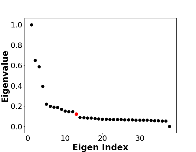
(a) MM Sampling

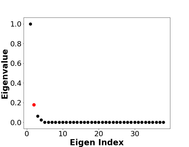
(b) k-means Sampling

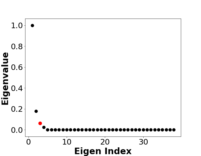
(c) DPP Sampling

(d) Random Sampling

Figure 1: Sorted and normalized eigenvalues of Banknote Authentication dataset with different sampling methods.

(e) MM Sampling

(f) k-means Sampling

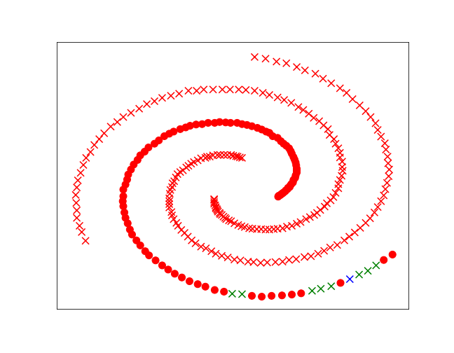
(g) DPP Sampling

(h) Random Sampling

Figure 2: Qualitative illustration on the Spiral dataset by different sampling methods.

Table 1: Quantitative results of different sampling schemes.

	Dataset	Metric	None	MM	k-means	DPP	Random
Synthetic Data	Pathbased	M1	62.11%	61.05%	47.27%	53.47%	00.22%
		M2	66.39 %	68.01%	52.20%	62.37%	00.10%
		M3	67.22%	70.20%	55.52%	65.81%	00.74 %
	Spiral	M1	100%	100%	08.21%	07.57%	00.24%
		M2	100 %	100%	10.55%	15.31%	00.26%
		M3	100%	100%	11.39%	17.25%	00.34 %
	Aggregation	M1	86.87%	80.45%	92.08%	84.78%	00.93%
		M2	87.69%	80.82%	91.19%	88.81%	01.14%
		M3	92.31%	90.31%	93.26%	92.24%	02.51%
Real Data	Banknote	M1	58.53%	58.11%	07.01 %	12.65%	00.06%
		M2	58.06%	52.26 %	05.00%	16.62%	00.00%
		M3	58.15%	52.33 %	05.84%	21.45%	00.06%
	Cloud	M1	100%	96.32%	73.00%	95.28%	00.01%
		M2	100%	93.33 %	68.53%	94.77%	00.00%
		M3	100%	93.32%	96.07%	93.18 %	00.00%
	Iris	M1	55.10%	66.37%	74.55%	64.10%	00.56%
		M2	58.26%	68.64%	78.79%	66.87%	00.40%
		M3	66.94%	71.74%	69.42%	70.48%	01.72%
	Perfume	M1	78.44 %	64.88%	59.75%	40.04%	00.08%
		M2	89.24%	74.28%	78.78%	51.22%	00.14%
		M3	92.48%	85.64%	81.44%	53.88%	12.76%
	Seed	M1	61.89%	48.26 %	75.25 %	65.52%	00.47%
		M2	57.55%	45.88%	70.44%	67.08%	00.69%
		M3	58.29%	50.73%	69.74%	69.83 %	01.73%
Image Data	Bottle 2009_002204	M1	70.15%	70.13%	64.39 %	53.12%	01.17%
		M2	56.30%	55.23%	48.05%	36.88%	00.37%
		M3	56.48%	56.33%	52.99%	41.20%	00.18%
	Bird 2011_001967	M1	66.89%	56.33%	54.33%	31.88%	01.30%
		M2	41.62%	32.30%	33.50%	18.72%	00.10 %
		M3	43.23%	37.59%	36.10%	20.29%	00.39%

Therefore, we apply GMM to the embedding vectors $\mathbf{E}_{d^{{}^{\prime}}}$ and then extend the sample labels to all the other objects represented by the corresponding sample. Finally, as shown in Table 1, we compare the estimated cluster labels with the ground truth labels. Table 1 shows the quantitative results of the different sampling methods. The None column refers to the no sampling case, where we use all the objects. In this case, we obtain Minimax distance matrix for all objects and apply GMM to the respective embedded vectors. Despite memory inefficiency, the results of this case provide information about effectiveness of sampling.

We observe that for two out of three synthetic datasets, MM Sampling outperforms the other methods. However, even for Aggregation dataset the results from MM Sampling are acceptable. Similarly, on UCI datasets, MM Sampling yields often the best or close to best results. Finally, on image segmentation, MM Sampling still achieves the best scores.

Qualitative results on the Spiral dataset are illustrated in Figure 2, where different colors denote different estimated clusters, and dots and crosses respectively indicate correctly and incorrectly labeled objects. Figure 1(e) shows GMM results obtained by MM Sampling, where all objects are correctly clustered. MM Sampling adapts well with the elongated structures in the data. Figure 1(f) and Figure 1(g) illustrate the clustering results with $k$-means and DPP sampling methods. Both methods mistakenly assign almost all data to a single cluster. Finally, Figure 1(h) shows the results of GMM with random sampling.

In terms of space complexity, random and MM Sampling satisfy a linear space complexity $\mathcal{O}\left(N\right)$. $k$-means sampling requires $\mathcal{O}\Big{(}N\big{(}D$+$K\big{)}\Big{)}$ memory, and as discussed, standard DPP requires computing samples offline with the space complexity of $\mathcal{O}\left(N^{2}\right)$.

5 Conclusion

We developed a generic framework for memory-efficient computation of Minimax distances based on effective sampling schemes. Within this framework, we developed an adaptive and memory-efficient sampling method consistent with the pairwise Minimax distances on the entire datasets. We evaluated the framework and the sampling methods on clustering of several datasets with GMM.

References

- [1] Ian J. Goodfellow, Yoshua Bengio, and Aaron C. Courville. Deep Learning. Adaptive computation and machine learning. MIT Press, 2016.
- [2] François Fouss, Kevin Francoisse, Luh Yen, Alain Pirotte, and Marco Saerens. An experimental investigation of kernels on graphs for collaborative recommendation and semisupervised classification. Neural Networks, 31:5372, 2012.
- [3] Pavel Chebotarev. A class of graph-geodetic distances generalizing the shortest-path and the resistance distances. Discrete Appl. Math., 159(5):295–302, 2011.
- [4] Bernd Fischer and Joachim M. Buhmann. Path-based clustering for grouping of smooth curves and texture segmentation. IEEE Trans. Pattern Anal. Mach. Intell., 25(4):513–518, 2003.
- [5] Morteza Haghir Chehreghani. Unsupervised representation learning with minimax distance measures. Machine Learning, 2020.
- [6] Kye-Hyeon Kim and Seungjin Choi. Walking on minimax paths for k-nn search. In Twenty-Seventh AAAI Conference on Artificial Intelligence, 2013.
- [7] Morteza Haghir Chehreghani. K-nearest neighbor search and outlier detection via minimax distances. In SIAM International Conference on Data Mining (SDM), pages 405–413, 2016.
- [8] Morteza Haghir Chehreghani. Feature-oriented analysis of user profile completion problem. In 39th European Conference on Information Retrieval (ECIR), pages 304–316, 2017.
- [9] Thomas H. Cormen, Clifford Stein, Ronald L. Rivest, and Charles E. Leiserson. Introduction to Algorithms. McGraw-Hill Higher Education, 2001.
- [10] Morteza Haghir Chehreghani. Classification with minimax distance measures. In Thirty-First AAAI Conference on Artificial Intelligence, pages 1784–1790, 2017.
- [11] Morteza Haghir Chehreghani. Efficient computation of pairwise minimax distance measures. In IEEE International Conference on Data Mining, ICDM, pages 799–804, 2017.
- [12] Gale Young and A. Householder. Discussion of a set of points in terms of their mutual distances. Psychometrika, 3(1):19–22, 1938.
- [13] Alex Kulesza and Ben Taskar. k-dpps: Fixed-size determinantal point processes. In ICML, pages 1193–1200, 2011.
- [14] Pasi Fränti and Sami Sieranoja. K-means properties on six clustering benchmark datasets, 2018.
- [15] Dheeru Dua and Casey Graff. UCI machine learning repository, 2017.
- [16] M. Everingham, L. Van Gool, C. K. I. Williams, J. Winn, and A. Zisserman. The PASCAL Visual Object Classes Challenge 2012 (VOC2012) Results. http://www.pascal-network.org/challenges/VOC/voc2012/workshop/index.html.