On the Likelihood of Local Projection Models

Abstract

A local projection model is defined by a set of linear regressions that account for the associations between exogenous variables and an endogenous variable observed at different time points. While it is standard practice to separately estimate individual regressions using the ordinary least squares estimator, some recent studies treat a local projection model as a multivariate regression with correlated errors, i.e., seemingly unrelated regressions, and propose Bayesian and non-Bayesian methods to improve the estimation accuracy. However, it is not clear how and when this way of treatment of local projection models is justified. The primary purpose of this paper is to fill this gap by showing that the likelihood of local projection models can be analytically derived from a stationary vector moving average process. By means of numerical experiments, we confirm that this treatment of local projections is tenable for finite samples.

Keywords:

local projections; system of equations; seemingly unrelated regressions

1 Introduction

Local projections (LPs) (Jordà, 2005) are linear regressions that project observations of an endogenous variable at different time periods, $y_{t},y_{t+1},...,y_{t+H}$, onto exogenous variables observed at period $t$, $\boldsymbol{x}_{t}$:

$$y_{t+h}=\boldsymbol{\theta}_{\left(h\right)}^{\top}\boldsymbol{x}_{t-1}+u_{\left(h\right),t+h},\quad h=0,1,...,H;\;t=1,...,T,$$ (1)

where $\boldsymbol{\theta}_{\left(h\right)}$ is a coefficient vector and $u_{\left(h\right),t+h}$ is a residual. $\boldsymbol{x}_{t-1}$ may include an intercept, preidentified structural shocks, the lags of the endogenous variables up to period $t-1$, and other controls. LPs are mainly employed for impulse response analysis. When the $n$th element of $\boldsymbol{x}_{t-1}$, denoted by $x_{n,t-1}$, is a preidentified structural shock, a sequence of the corresponding coefficients is interpreted as an impulse response function, namely,

$$\theta_{\left(h\right),n}=\partial y_{t+h}/\partial x_{n,t-1},\quad h=0,1,...,H.$$

Because of their flexibility and robustness to model misspecification, LPs are extensively applied to investigate the economic dynamics (e.g., Ramey2016a and cited therein). In this paper, we refer to a set of LPs for the same endogenous variable (1) as an LP model and statistical analysis using an LP model as the LP method.

The LP method is intrinsically different from conventional approaches to time series modeling. Standard time series models, such as the vector autoregressive (VAR) model and its variants, are designed to approximate the data generating process (DGP). In contrast, the LP method does not explicitly assume the DGP and directly captures the associations between the exogenous variables $\boldsymbol{x}_{t-1}$ and the endogenous variable observed at different time points $y_{t+h}$, $h=0,1,...,H$.

It is standard practice to separately estimate LPs (1) using the ordinary least squares (OLS) estimator, while Tanaka (2020) and El-Shagi (2019) estimate an LP model as a multivariate regression with correlated residuals, i.e., seemingly unrelated regressions (SUR) (Zellner, 1962). Tanaka (2020) and El-Shagi (2019) treat response variables for different projection horizons as correlated but different variables and estimate an LP model as a multivariate regression model where a vector of the responses $\boldsymbol{y}_{t}=\left(y_{t},y_{t+1},...,y_{t+H}\right)^{\top}$ are regressed on the covariates $\boldsymbol{x}_{t-1}$:

$$\boldsymbol{y}_{t}=\boldsymbol{\Theta}^{\top}\boldsymbol{x}_{t-1}+\boldsymbol{u}_{t},\quad t=1,...,T,$$ (2)

$$\boldsymbol{u}_{t}=\left(u_{t},u_{t+1},...,u_{t+H}\right)^{\top},\quad t=1,...,T,$$

$$\boldsymbol{\Theta}=\left(\boldsymbol{\theta}_{\left(0\right)},\boldsymbol{\theta}_{\left(1\right)},...,\boldsymbol{\theta}_{\left(H\right)}\right).$$

Tanaka (2020) assumes that the residuals of an LP model are distributed according to a multivariate normal distribution with the covariance matrix $\boldsymbol{\Sigma}$, $\boldsymbol{u}_{t}\sim\mathcal{N}\left(\boldsymbol{0}_{H+1},\boldsymbol{\Sigma}\right)$, where $\mathcal{N}\left(\boldsymbol{a},\boldsymbol{B}\right)$ denotes a multivariate normal distribution with mean $\boldsymbol{a}$ and covariance matrix $\boldsymbol{B}$. Thus, the (conditional) distribution of $\boldsymbol{y}_{t}$ is specified as

$$\left(\boldsymbol{y}_{t}|\boldsymbol{x}_{t-1};\boldsymbol{\Theta},\boldsymbol{\Sigma}\right)\sim\mathcal{N}\left(\boldsymbol{\Theta}^{\top}\boldsymbol{x}_{t-1},\;\boldsymbol{\Sigma}\right),\quad t=1,...,T,$$ (3)

which leads to the following likelihood:

$$p\left(\boldsymbol{Y}|\boldsymbol{\Theta},\boldsymbol{\Sigma},\boldsymbol{X}\right) = \prod_{t=1}^{T}p\left(\boldsymbol{y}_{t}|\boldsymbol{x}_{t-1};\boldsymbol{\Theta},\boldsymbol{\Sigma}\right)$$

$$= \prod_{t=1}^{T}f_{N}\left(\boldsymbol{y}_{t}|\boldsymbol{\Theta}^{\top}\boldsymbol{x}_{t-1},\boldsymbol{\Sigma}\right)$$

$$= \left(2\pi\right)^{-\frac{\left(H+1\right)T}{2}}\left|\boldsymbol{\Sigma}\right|^{-\frac{T}{2}}\exp\left[-\frac{1}{2}\sum_{t=1}^{T}\left(\boldsymbol{y}_{t}-\boldsymbol{\Theta}^{\top}\boldsymbol{x}_{t-1}\right)^{\top}\boldsymbol{\Sigma}^{-1}\left(\boldsymbol{y}_{t}-\boldsymbol{\Theta}^{\top}\boldsymbol{x}_{t-1}\right)\right],$$

$$\boldsymbol{Y}=\left(\boldsymbol{y}_{1},...,\boldsymbol{y}_{T}\right)^{\top},\quad\boldsymbol{X}=\left(\boldsymbol{x}_{1},...,\boldsymbol{x}_{T}\right)^{\top}.$$

where $f_{N}\left(\boldsymbol{a}|\boldsymbol{b},\boldsymbol{C}\right)$ denotes the probability density function of a multivariate normal distribution with mean $\boldsymbol{b}$ and covariance matrix $\boldsymbol{C}$ evaluated at $\boldsymbol{a}$. Tanaka (2020) considers Bayesian inference of LP models based on this likelihood. El-Shagi (2019) estimates LP models in a similar way to a feasible generalized least-squares estimation of an SUR model, where the quadratic loss function that he employs is closely related to the previously described likelihood (1). Tanaka (2020) and El-Shagi (2019) propose a Bayesian approach and a non-Bayesian approach to improve the estimation of accuracy using a tailored prior and a penalty term, respectively.

Whereas Tanaka (2020) and El-Shagi (2019) show that their statistical approaches perform well by means of simulation studies, they do not explicitly discuss how and when the likelihood of the LP models that they utilize (1) is justified. The primary focus of this paper is to fill this gap. We suggest that their SUR-like treatment of LP models is statistically valid by showing that the likelihood (1) can be analytically derived from a stationary vector moving average (VMA) process with the normality assumption.

Lusompa (2019) proposes Bayesian and non-Bayesian methods to estimate LPs. Unlike the SUR-like treatment in Tanaka (2020) and El-Shagi (2019), his approach requires estimation of all the LPs for endogenous variables, i.e., the whole system of LPs; thus, it is computationally demanding. Specifically, his Bayesian method is not practical when the number of endogenous variables and/or the number of projection horizons is large. In most situations, it is not necessary to examine all the LPs because analysts’ attention is limited to coefficients that represent impulse responses of interest. Thus, confirming the statistical validity of the SUR-like treatment of LPs in Tanaka (2020) and El-Shagi (2019), which is more parsimonious than that of Lusompa (2019), has practical importance.

We discuss the relationship between a VMA process and the SUR-like likelihood of an LP model in two steps. First, we develop the entire system of LPs from a stationary VMA process with normality assumption (Section 2). Second, we define an LP model as a sub-system of the entire system of LPs and derive its probabilistic representation, i.e., the likelihood (Section 3). We see that the covariance matrix of the residuals of an LP model can be represented as a (matrix-valued) function of the parameters of the VMA process and that it is non-diagonal, full rank, and symmetric positive definite. Therefore, the likelihood of an LP model can be specified as in SUR. By means of numerical experiments, we show that the derived representation of the residual covariance matrix can be accurately estimated using the OLS estimator and Bayesian Markov chain Monte Carlo method (Section 4). Therefore, the SUR-like treatment of LP models is tenable for finite samples.

2 From VMA Process to Entire System of LPs

This section derives an entire system of LPs that corresponds to the underlying DGP specified by a VMA process. We assume that data $\left\{\boldsymbol{w}_{t}\right\}$ are generated from an $L$th-order stationary VMA process:

$$\boldsymbol{w}_{t}=\boldsymbol{\varepsilon}_{t}+\sum_{l=1}^{L}\boldsymbol{\Gamma}_{l}\boldsymbol{\varepsilon}_{t-l},\quad\boldsymbol{\varepsilon}_{t}\sim\mathcal{N}\left(\boldsymbol{0}_{M},\boldsymbol{\Omega}_{\varepsilon}\right),\quad t=-\infty,...,T,$$ (5)

where $\boldsymbol{w}_{t}=\left(w_{t}^{\left\langle 1\right\rangle},...,w_{t}^{\left\langle M\right\rangle}\right)^{\top}$ is an $M$-dimensional vector of endogenous variables, $\boldsymbol{\varepsilon}_{t}$ is an $M$-dimensional vector of structural shocks that are distributed according to a multivariate normal distribution with covariance matrix $\boldsymbol{\Omega}_{\boldsymbol{\varepsilon}}$, and $\boldsymbol{\Gamma}_{l}$ is an $M$-by-$M$ VMA coefficient matrix. Without loss of generality, intercepts are omitted. The process is not assumed to be fundamental; thus, our discussion applies not only to VAR processes but also to more general multivariate time series. The identification of structural shocks is beyond the scope of this paper; impulse responses can be estimated only when the shocks are exogenous or identified before inference.

An $h$ horizon LP is defined by a projection of $\boldsymbol{w}_{t+h}$ onto the lags of the endogenous variables, $\boldsymbol{w}_{t-1},...,\boldsymbol{w}_{t-L}$:

$$\boldsymbol{w}_{t+h}=\textrm{Proj}\left(\boldsymbol{w}_{t+h}|\boldsymbol{w}_{t-1},...,\boldsymbol{w}_{t-L}\right)+\boldsymbol{e}_{\left(h\right),t+h},\quad=0,1,...,H;\;t=1,...,T,$$ (6)

where $\textrm{Proj}\left(\boldsymbol{a}|\boldsymbol{b}\right)$ denotes the orthogonal projection of $\boldsymbol{a}$ onto $\boldsymbol{b}$ and $\boldsymbol{e}_{\left(h\right),t+h}=\left(e_{\left(h\right),t+h}^{\left\langle 1\right\rangle},...,e_{\left(h\right),t+h}^{\left\langle M\right\rangle}\right)^{\top}$ is an $M$-dimensional vector of the LP residuals. The orthogonal projection $\textrm{Proj}\left(\boldsymbol{w}_{t+h}|\boldsymbol{w}_{t-1},...,\boldsymbol{w}_{t-L}\right)$ is specified by the linear projection $\sum_{l=1}^{L}\left[\boldsymbol{\Phi}_{\left(h+1\right),l}\boldsymbol{w}_{t-l}\right]$, where $\boldsymbol{\Phi}_{\left(h\right),l}$ is an $M$-by-$M$ LP coefficient matrix whose $\left(m,n\right)$-element is denoted by $\phi_{\left(h\right),l}^{\left\langle m\right\rangle\left\langle n\right\rangle}$. Each LP is posed as

$$\boldsymbol{w}_{t+h}=\sum_{l=1}^{L}\left[\boldsymbol{\Phi}_{\left(h+1\right),l}\boldsymbol{w}_{t-l}\right]+\boldsymbol{e}_{\left(h\right),t+h},\quad h=0,1,...,H;\;t=1,...,T.$$

In the following section, we refer to this representation of LPs (or equivalently (6)) as the entire system of LPs, in distinction from an LP model for a specific endogenous variable, such as (1) and (2). Although multivariate time series data are considered, an LP model is not a typical time series model. The purpose of the model is to directly examine the relationship between variables measured at different time points, not to recover the underlying DGP.

The construction of the likelihood of LP models is different from that of the standard multivariate time series models. For instance, if the VMA process (5) has a VAR representation, the likelihood of the VAR model is written generically in the following form:

$$p\left(\boldsymbol{W}|\mathcal{P}_{VAR}\right)=\prod_{t}p\left(\boldsymbol{w}_{t}|\boldsymbol{w}_{t-1},...,\boldsymbol{w}_{t-L};\mathcal{P}_{VAR}\right),$$

where $\mathcal{P}_{VAR}$ denotes a set of parameters that specify the VAR model. Contrastingly, the likelihood of the LP representation of the VMA process (6) is specified as

$$p\left(\boldsymbol{W}|\mathcal{P}_{LP}\right)=\prod_{m=1}^{M}\prod_{t=1}^{T}\prod_{h=0}^{H}p\left(w_{t+h}^{\left\langle m\right\rangle}|\boldsymbol{w}_{t-1},...,\boldsymbol{w}_{t-L};\mathcal{P}_{LP}\right),$$

where $\mathcal{P}_{LP}$ denotes a set of parameters that specify the entire system of LPs. As shown in Jordà (2005), when the true DGP is a VAR process, the LP coefficients $\boldsymbol{\Phi}_{\left(h+1\right),l}$, $l=1,...,L$, are parametrized by the coefficients that specify the VAR process.

The residuals of the entire system of LPs $\boldsymbol{e}_{\left(h\right),t+h}$ have autocorrelations. Lusompa (2019) shows that the process of $\boldsymbol{e}_{\left(h\right),t+h}$ is known: for $t=1,...,T$,

$$\boldsymbol{e}_{\left(h\right),t+h}=\begin{cases}\boldsymbol{v}_{\left(h\right),t+h},&h=0,\\ \sum_{i=1}^{h}\left[\boldsymbol{\Gamma}_{i}\boldsymbol{\varepsilon}_{t+h-i}\right]+\boldsymbol{v}_{\left(h\right),t+h},&h=1,...,H,\end{cases}$$

where $\boldsymbol{v}_{\left(h\right),t+h}$ is an $M$-dimensional vector of serially uncorrelated residuals. In the population, it follows that

$$\boldsymbol{v}_{\left(h\right),t+h} = \boldsymbol{\varepsilon}_{t+h},\quad h=0,1,...,H;\;t=1,...,T,$$

$$\boldsymbol{\Phi}_{\left(h\right),1} = \boldsymbol{\Gamma}_{h},\quad h=1,...,H.$$

The residuals are written as

$$\boldsymbol{e}_{\left(h\right),t+h} = \begin{cases}\boldsymbol{\varepsilon}_{t},&h=0,\\ \sum_{i=1}^{h}\left[\boldsymbol{\Phi}_{\left(h\right),1}\boldsymbol{\varepsilon}_{t+h-i}\right]+\boldsymbol{\varepsilon}_{t+h},&h=1,...,H,\end{cases}$$ (7)

for $t=1,...,T$.

3 From Entire System of LPs to LP model

An LP model for the $m$th endogenous variable is defined by extracting a portion of the LPs, or a sub-system, from the remainder of the entire system:

$$w_{t+h}^{\left\langle m\right\rangle}=\sum_{l=1}^{L}\left[\left(\boldsymbol{\Phi}_{l}^{\left\langle m\right\rangle}\right)^{\top}\boldsymbol{w}_{t-l}\right]+e_{\left(h\right),t+h}^{\left\langle m\right\rangle},\quad h=0,1,...,H;\;t=1,...,T,$$

$$\boldsymbol{\Phi}_{l}^{\left\langle m\right\rangle}=\left(\boldsymbol{\phi}_{\left(0\right),l}^{\left\langle m\right\rangle},\boldsymbol{\phi}_{\left(1\right),l}^{\left\langle m\right\rangle},...,\boldsymbol{\phi}_{\left(H\right),l}^{\left\langle m\right\rangle}\right),\quad l=1,...,L,$$

where $\boldsymbol{\phi}_{\left(h\right),l}^{\left\langle m\right\rangle}$ is a vector containing the element of the $m$th row of $\boldsymbol{\Phi}_{\left(h\right),l}$. This sub-system is summarized in an analogous fashion to (2): for $t=1,...,T$,

$$\boldsymbol{w}_{t}^{\left\langle m\right\rangle}=\left(\boldsymbol{\Phi}^{\left\langle m\right\rangle}\right)^{\top}\tilde{\boldsymbol{w}}_{t-1}+\boldsymbol{e}_{t}^{\left\langle m\right\rangle},$$

$$\boldsymbol{w}_{t}^{\left\langle m\right\rangle}=\left(w_{t}^{\left\langle m\right\rangle},w_{t+1}^{\left\langle m\right\rangle},...,w_{t+H}^{\left\langle m\right\rangle}\right)^{\top},\quad t=1,...,T,$$

$$\tilde{\boldsymbol{w}}_{t-1}=\left(\boldsymbol{w}_{t-1}^{\top},...,\boldsymbol{w}_{t-L}^{\top}\right)^{\top},$$

$$\boldsymbol{e}_{t}^{\left\langle m\right\rangle}=\left(e_{t}^{\left\langle m\right\rangle},e_{t+1}^{\left\langle m\right\rangle},...,e_{t+H}^{\left\langle m\right\rangle}\right)^{\top},$$

$$\boldsymbol{\Phi}^{\left\langle m\right\rangle}=\left(\begin{array}[]{c}\boldsymbol{\Phi}_{1}^{\left\langle m\right\rangle}\\ \vdots\\ \boldsymbol{\Phi}_{L}^{\left\langle m\right\rangle}\end{array}\right),$$

The likelihood of the sub-system is structured as

$$p\left(\boldsymbol{W}^{\left\langle m\right\rangle}|\mathcal{P}_{LP}\right) = \prod_{t=1}^{T}\prod_{h=0}^{H}p\left(w_{t+h}^{\left\langle m\right\rangle}|\boldsymbol{w}_{t-1},...,\boldsymbol{w}_{t-L};\mathcal{P}_{LP}\right)$$

$$= \prod_{t=1}^{T}p\left(\boldsymbol{w}_{t}^{\left\langle m\right\rangle}|\boldsymbol{w}_{t-1},...,\boldsymbol{w}_{t-L};\mathcal{P}_{LP}\right),$$

$$\boldsymbol{W}^{\left\langle m\right\rangle}=\left(\boldsymbol{w}_{1}^{\left\langle m\right\rangle},...,\boldsymbol{w}_{T}^{\left\langle m\right\rangle}\right)^{\top}.$$

This expression corresponds to (1).

In the following section, we show that the residuals of the sub-system are distributed according to a multivariate distribution, $\boldsymbol{e}_{t}^{\left\langle m\right\rangle}\sim\mathcal{N}\left(\boldsymbol{0}_{H+1},\boldsymbol{\Xi}\right)$, where $\boldsymbol{\Xi}$ is a symmetric positive definite matrix, and that the distribution of $\boldsymbol{w}_{t}^{\left\langle m\right\rangle}$ is specified as

$$\left(\boldsymbol{w}_{t}^{\left\langle m\right\rangle}|\tilde{\boldsymbol{w}}_{t-1};\boldsymbol{\Phi}^{\left\langle m\right\rangle},\boldsymbol{\Sigma}\right)\sim\mathcal{N}\left(\left(\boldsymbol{\Phi}^{\left\langle m\right\rangle}\right)^{\top}\tilde{\boldsymbol{w}}_{t-1},\;\boldsymbol{\Xi}\right),\quad t=1,...,T.$$ (9)

This expression is a mirror image of (3). We analytically derive the covariance of the residuals of the sub-system $\boldsymbol{e}_{t}^{\left\langle m\right\rangle}$ as a matrix-valued function of the parameters of the LP coefficients for the $m$th endogenous variable and the covariance of the structural shocks $\boldsymbol{\Omega}_{\boldsymbol{\varepsilon}}$, which shows that $\boldsymbol{\Xi}$ is proper as a covariance matrix because it is full rank, symmetric, and positive definite. For readers’ convenience, the correspondence between the notations in the SUR-like treatment of an LP model (1) and the VMA process is summarized in Table 1.

From (7), using the LP coefficients and the structural shocks, the residuals can be rewritten as follows:

$$\boldsymbol{e}_{t}^{\left\langle m\right\rangle} = \left(\begin{array}[]{c}e_{\left(0\right),t}^{\left\langle m\right\rangle}\\ e_{\left(1\right),t+1}^{\left\langle m\right\rangle}\\ e_{\left(2\right),t+2}^{\left\langle m\right\rangle}\\ \vdots\\ e_{\left(H\right),t+H}^{\left\langle m\right\rangle}\end{array}\right)$$

$$= \left(\begin{array}[]{c}\varepsilon_{t}^{\left\langle m\right\rangle}\\ \left(\boldsymbol{\phi}_{\left(1\right),1}^{\left\langle m\right\rangle}\right)^{\top}\boldsymbol{\varepsilon}_{t}+\varepsilon_{t+1}^{\left\langle m\right\rangle}\\ \left(\boldsymbol{\phi}_{\left(2\right),1}^{\left\langle m\right\rangle}\right)^{\top}\boldsymbol{\varepsilon}_{t}+\left(\boldsymbol{\phi}_{\left(1\right),1}^{\left\langle m\right\rangle}\right)^{\top}\boldsymbol{\varepsilon}_{t+1}+\varepsilon_{t+2}^{\left\langle m\right\rangle}\\ \vdots\\ \left(\boldsymbol{\phi}_{\left(H\right),1}^{\left\langle m\right\rangle}\right)^{\top}\boldsymbol{\varepsilon}_{t}+\left(\boldsymbol{\phi}_{\left(H-1\right),1}^{\left\langle m\right\rangle}\right)^{\top}\boldsymbol{\varepsilon}_{t+1}+\cdots+\left(\boldsymbol{\phi}_{\left(1\right),1}^{\left\langle m\right\rangle}\right)^{\top}\boldsymbol{\varepsilon}_{t+H-1}+\varepsilon_{t+H}^{\left\langle m\right\rangle}\end{array}\right).$$

Let $\boldsymbol{\iota}_{m}$ denote an $M$-dimensional vector of zeros, where the $m$th element is replaced by one. The residuals are arranged as

$$\boldsymbol{e}_{t}^{\left\langle m\right\rangle} = \left(\begin{array}[]{c}\boldsymbol{\iota}_{m}^{\top}\boldsymbol{\varepsilon}_{t}\\ \left(\boldsymbol{\phi}_{\left(1\right),1}^{\left\langle m\right\rangle}\right)^{\top}\boldsymbol{\varepsilon}_{t}+\boldsymbol{\iota}_{m}^{\top}\boldsymbol{\varepsilon}_{t+1}\\ \left(\boldsymbol{\phi}_{\left(2\right),1}^{\left\langle m\right\rangle}\right)^{\top}\boldsymbol{\varepsilon}_{t}+\left(\boldsymbol{\phi}_{\left(1\right),1}^{\left\langle m\right\rangle}\right)^{\top}\boldsymbol{\varepsilon}_{t+1}+\boldsymbol{\iota}_{m}^{\top}\boldsymbol{\varepsilon}_{t+2}\\ \vdots\\ \left(\boldsymbol{\phi}_{\left(H\right),1}^{\left\langle m\right\rangle}\right)^{\top}\boldsymbol{\varepsilon}_{t}+\left(\boldsymbol{\phi}_{\left(H-1\right),1}^{\left\langle m\right\rangle}\right)^{\top}\boldsymbol{\varepsilon}_{t+1}+\cdots+\left(\boldsymbol{\phi}_{\left(1\right),1}^{\left\langle m\right\rangle}\right)^{\top}\boldsymbol{\varepsilon}_{t+H-1}+\boldsymbol{\iota}_{m}^{\top}\boldsymbol{\varepsilon}_{t+H}\end{array}\right)$$

$$= \left(\begin{array}[]{ccccc}\boldsymbol{\iota}_{m}^{\top}\\ \left(\boldsymbol{\phi}_{\left(1\right),1}^{\left\langle m\right\rangle}\right)^{\top}&\boldsymbol{\iota}_{m}^{\top}\\ \left(\boldsymbol{\phi}_{\left(2\right),1}^{\left\langle m\right\rangle}\right)^{\top}&\left(\boldsymbol{\phi}_{\left(1\right),1}^{\left\langle m\right\rangle}\right)^{\top}&\boldsymbol{\iota}_{m}^{\top}\\ \vdots&\vdots&\cdot&\ddots\\ \left(\boldsymbol{\phi}_{\left(H\right),1}^{\left\langle m\right\rangle}\right)^{\top}&\left(\boldsymbol{\phi}_{\left(H-1\right),1}^{\left\langle m\right\rangle}\right)^{\top}&\cdots&\left(\boldsymbol{\phi}_{\left(1\right),1}^{\left\langle m\right\rangle}\right)^{\top}&\boldsymbol{\iota}_{m}^{\top}\end{array}\right)\left(\begin{array}[]{c}\boldsymbol{\varepsilon}_{t}\\ \boldsymbol{\varepsilon}_{t+1}\\ \boldsymbol{\varepsilon}_{t+2}\\ \vdots\\ \boldsymbol{\varepsilon}_{t+H}\end{array}\right).$$

The covariance of $\boldsymbol{e}_{t}^{\left\langle m\right\rangle}$ is represented using the LP coefficients and the covariance matrix of the structural shocks as

$$\boldsymbol{\Xi}=\bar{\boldsymbol{\Phi}}^{\left\langle m\right\rangle}\left(\boldsymbol{I}_{H+1}\otimes\boldsymbol{\Omega}_{\varepsilon}\right)\left(\bar{\boldsymbol{\Phi}}^{\left\langle m\right\rangle}\right)^{\top},$$ (14)

$$\bar{\boldsymbol{\Phi}}^{\left\langle m\right\rangle}=\left(\begin{array}[]{ccccc}\boldsymbol{\iota}_{m}^{\top}\\ \left(\boldsymbol{\phi}_{\left(1\right),1}^{\left\langle m\right\rangle}\right)^{\top}&\boldsymbol{\iota}_{m}^{\top}\\ \left(\boldsymbol{\phi}_{\left(2\right),1}^{\left\langle m\right\rangle}\right)^{\top}&\left(\boldsymbol{\phi}_{\left(1\right),1}^{\left\langle m\right\rangle}\right)^{\top}&\boldsymbol{\iota}_{m}^{\top}\\ \vdots&\vdots&\cdot&\ddots\\ \left(\boldsymbol{\phi}_{\left(H\right),1}^{\left\langle m\right\rangle}\right)^{\top}&\left(\boldsymbol{\phi}_{\left(H-1\right),1}^{\left\langle m\right\rangle}\right)^{\top}&\cdots&\left(\boldsymbol{\phi}_{\left(1\right),1}^{\left\langle m\right\rangle}\right)^{\top}&\boldsymbol{\iota}_{m}^{\top}\end{array}\right).$$ (15)

This expression implies that $\boldsymbol{\Xi}$ is non-diagonal, full rank, and symmetric positive definite. Thus, $\boldsymbol{\Xi}$ is properly defined as a covariance matrix, and the distribution of $\boldsymbol{w}_{t}^{\left\langle m\right\rangle}$ can be written in the form of (9).

Given $\boldsymbol{\Omega}_{\boldsymbol{\varepsilon}}$, the likelihood of this sub-system is independent from the VMA coefficients for the remainder of the whole system (6), because $\bar{\boldsymbol{\Phi}}^{\left\langle m\right\rangle}$ does not contain the LP coefficients for the remaining endogenous variables, namely, $\boldsymbol{\phi}_{\left(h\right),1}^{\left\langle m^{\prime}\right\rangle}$, $h=0,1,...,H$; $m^{\prime}\neq m$. Therefore, to recover the LP coefficients from the data, it is sufficient to estimate the sub-system. The likelihood (3) is specified as follows:

$$p\left(\boldsymbol{W}^{\left\langle m\right\rangle}|\boldsymbol{\Phi}^{\left\langle m\right\rangle},\boldsymbol{\Xi}\right) = \prod_{t=1}^{T}p\left(\boldsymbol{w}_{t}^{\left\langle m\right\rangle}|\tilde{\boldsymbol{w}}_{t-1};\boldsymbol{\Phi}^{\left\langle m\right\rangle},\boldsymbol{\Xi}\right)$$

$$= \prod_{t=1}^{T}f_{N}\left(\boldsymbol{w}_{t}^{\left\langle m\right\rangle}|\left(\boldsymbol{\Phi}^{\left\langle m\right\rangle}\right)^{\top}\tilde{\boldsymbol{w}}_{t-1},\;\boldsymbol{\Xi}\right)$$

$$= \left(2\pi\right)^{-\frac{\left(H+1\right)T}{2}}\left|\boldsymbol{\Xi}\right|^{-\frac{T}{2}}\exp\left[-\frac{1}{2}\sum_{t=1}^{T}\left(\boldsymbol{w}_{t}^{\left\langle m\right\rangle}-\left(\boldsymbol{\Phi}^{\left\langle m\right\rangle}\right)^{\top}\tilde{\boldsymbol{w}}_{t-1}\right)^{\top}\right.$$

$$\hskip 150.5625pt\left.\boldsymbol{\Xi}^{-1}\left(\boldsymbol{w}_{t}^{\left\langle m\right\rangle}-\left(\boldsymbol{\Phi}^{\left\langle m\right\rangle}\right)^{\top}\tilde{\boldsymbol{w}}_{t-1}\right)\right]$$

There is a correspondence between this likelihood presentation and the SUR-like likelihood (1).

From the foregoing analysis, we confirm that the probabilistic representations of an LP model in (9), and thus, (3) are justifiable when the true DGP is a stationary VMA process with the normality assumption and that the likelihood of an LP model based on the SUR-like treatment (1), which is applied in Tanaka (2020), is statistically valid.

Lusompa (2019) proposes a Bayesian method to estimate the entire system of LPs (6). His posterior simulation algorithm consists of two steps. First, the horizon 0 LP, which is equivalent to a VAR model, is estimated. Second, for each draw, the remaining coefficients are simulated from the conditional posteriors sequentially for $h=1,2,...,H$. This algorithm is computationally demanding, because all the coefficient matrices of the entire system are inferred. In most situations, the analyst’s focus is limited to a small portion of these matrices, e.g., coefficients that represent impulse responses of interest. Thus, inference about the whole system is unnecessary. As long as structural shocks of interest are identified before inference, the SUR-like treatment of LPs is advantageous to the approach of Lusompa (2019).

4 Numerical Illustration

By numerical experiments, we investigate the small-sample performance of non-Bayesian and Bayesian approaches in the inference of an LP model. Synthetic data are generated from the following VMA process:

$$\boldsymbol{w}_{t}=\boldsymbol{\varepsilon}_{t}+\sum_{l=1}^{L}\boldsymbol{\Gamma}_{l}\boldsymbol{\varepsilon}_{t-l},\quad\boldsymbol{\varepsilon}_{t}\sim\mathcal{N}\left(\boldsymbol{0}_{M},\boldsymbol{\Omega}_{\varepsilon}\right).$$

We fix $M=3$, $L=5$, $H=7$, and $T=200$. Our focus is inference of the responses of the second element of $\boldsymbol{w}_{t}$ to the first element of $\boldsymbol{w}_{t}$, which is exogenous to the system. A covariate vector $\boldsymbol{x}_{t}$ includes $L$ lags of $\boldsymbol{w}_{t}$ and an intercept. The parameters for the synthetic data are randomly generated. Let $\gamma_{i,j,l}$ denote the $\left(i,j\right)$-element of $\boldsymbol{\Gamma}_{l}.$ The first element of $\boldsymbol{w}_{t}$ is a preidentified structural shock $w_{1,t}=\varepsilon_{1,t}$; thus, all the first rows of $\boldsymbol{\Gamma}_{l}$ are zero. A sequence of the $\left(2,1\right)$-elements of $\boldsymbol{\Gamma}_{l}$, which is denoted by $\boldsymbol{\gamma}_{IRF}=\left\{\gamma_{2,1,1},...,\gamma_{2,1,L}\right\}$, represents the impulse responses of interest. The elements of $\boldsymbol{\gamma}_{IRF}$ are specified as

$$\gamma_{2,1,l}=\frac{l\exp\left(d\left(1-l\right)\right)}{\sum_{l=1}^{L}l\exp\left(d\left(1-l\right)\right)},\quad l=1,...,L,$$

where $d$ is a parameter that controls the shape of the impulse response function. We fix $d=0.8$. The diagonal elements of $\boldsymbol{\Gamma}_{1}$ are uniformly sampled from the unit interval, $\left(0,1\right)$. The second to third rows of $\boldsymbol{\Gamma}_{l}$ are set to $\boldsymbol{\Gamma}_{2:3,1:3,l}=0.5\left(L-l\right)L^{-1}\boldsymbol{\Gamma}^{*}$, where each entry of $\boldsymbol{\Gamma}^{*}$ is independently generated from the standard normal distribution. The covariance matrix of $\boldsymbol{\varepsilon}_{t}$ is specified by $\boldsymbol{\Omega}_{\varepsilon}=\textrm{blkdiag}\left(\omega_{1}^{2},\boldsymbol{\Omega}_{\boldsymbol{\varepsilon}}^{*}\right)$. $\omega_{1}^{2}$ is simulated from an inverse gamma distribution with a shape parameter of 1 and scale parameter of 1, while $\boldsymbol{\Omega}_{\boldsymbol{\varepsilon}}^{*}$ is simulated from an inverse Wishart distribution with scale matrix $\boldsymbol{I}_{2}$ and $2$ degrees of freedom.

First, we consider a feasible generalized least-squares estimator, as discussed in El-Shagi (2019). In the first step, $\boldsymbol{\Theta}$ is estimated using the OLS estimator,

$$\hat{\boldsymbol{\Theta}}=\left(\boldsymbol{X}^{\top}\boldsymbol{X}\right)^{-1}\boldsymbol{X}^{\top}\boldsymbol{Y},$$

where $\boldsymbol{Y}=\left(\boldsymbol{y}_{1},...,\boldsymbol{y}_{T}\right)^{\top}$ and $\boldsymbol{X}=\left(\boldsymbol{x}_{0},\boldsymbol{x}_{1},...,\boldsymbol{x}_{T-1}\right)^{\top}$. Second, $\boldsymbol{\Sigma}$ is estimated based on the OLS residuals,

$$\hat{\boldsymbol{\Sigma}}=T^{-1}\left(\boldsymbol{Y}-\boldsymbol{X}\hat{\boldsymbol{\Theta}}\right)^{\top}\left(\boldsymbol{Y}-\boldsymbol{X}\hat{\boldsymbol{\Theta}}\right).$$

The second-step estimate of $\boldsymbol{\Theta}$ is obtained using $\hat{\boldsymbol{\Sigma}}$. The system might be re-estimated iteratively. The validity of this approach hinges critically on the precision of $\hat{\boldsymbol{\Sigma}}$. The parameters $\boldsymbol{\Gamma}_{l}$ and $\boldsymbol{\Sigma}_{\boldsymbol{\varepsilon}}$ are generated once and are fixed throughout the experiment, while the structural shocks $\boldsymbol{\varepsilon}_{t}$ are randomly generated for each trial. Figures 1–3 compare $\hat{\boldsymbol{\Sigma}}$ for 1,000 synthetic data with the true value of $\boldsymbol{\Sigma}$ given by (14) and (15). Vertical lines denote the true values, and the histograms represent the OLS estimates of $\boldsymbol{\Sigma}$ for different data. As evident from these figures, $\boldsymbol{\Sigma}$ can be consistently estimated based on the OLS residuals. Figure 4 shows histograms of the estimates of $\boldsymbol{\gamma}_{IRF}$. We see that $\boldsymbol{\gamma}_{IRF}$ can be estimated by the OLS estimator.

Next, in a similar vein, we consider the Bayesian inference of an LP model. To minimize the influence of priors on the posterior, we employ a flat prior for $\boldsymbol{\Theta}$, $p\left(\boldsymbol{\Theta}\right)\propto 1$, and a scale-invariant Jeffreys prior for $\boldsymbol{\Sigma}$, $p\left(\boldsymbol{\Sigma}\right)\propto\left|\boldsymbol{\Sigma}\right|^{-\left(H+2\right)/2}$. Posterior draws are simulated using a Gibbs sampler, and the conditionals are specified as

$$\textrm{vec}\left(\boldsymbol{\Theta}\right)|\boldsymbol{\Sigma},\boldsymbol{Y},\boldsymbol{X}\sim\mathcal{N}\left(\boldsymbol{m},\boldsymbol{P}^{-1}\right),$$

$$\boldsymbol{m}=\boldsymbol{P}^{-1}\left(\boldsymbol{\Sigma}^{-1}\otimes\boldsymbol{X}^{\top}\right)\textrm{vec}\left(\boldsymbol{Y}\right),$$

$$\boldsymbol{P}=\boldsymbol{\Sigma}^{-1}\otimes\boldsymbol{X}^{\top}\boldsymbol{X},$$

$$\boldsymbol{\Sigma}|\boldsymbol{\Theta},\boldsymbol{Y},\boldsymbol{X}\sim\mathcal{IW}\left(T,\;\left(\boldsymbol{Y}-\boldsymbol{X}\boldsymbol{\Theta}\right)^{\top}\left(\boldsymbol{Y}-\boldsymbol{X}\boldsymbol{\Theta}\right)\right),$$

where $\mathcal{IW}\left(a,\boldsymbol{B}\right)$ denotes an inverse Wishart distribution with $a$ degrees of freedom and scale matrix $\boldsymbol{B}$. We generate 11,000 draws and use the last 10,000 draws for the posterior analysis. All the chains in the experiments passed the Geweke (1992) test at the 5 percent level. Figures 5–7 contain histograms of the posterior mean estimates of $\boldsymbol{\Sigma}$. As with the OLS estimator, the posterior means of $\boldsymbol{\Sigma}$ are distributed around the true values. Figure 8 depicts histograms of the posterior mean estimates of the impulse responses of interest. The estimated impulse responses are distributed around the true values. Therefore, Bayesian analysis based on the SUR-like treatment of LP models is tenable for finite samples.

Correspondence of notations

Description	Notations in LP model		Notations in VMA process
Endogenous variable of interest	$y_{t+h}$	$\Leftrightarrow$	$w_{t+h}^{\left\langle m\right\rangle}$
Vector of endogenous variable of interest	$\boldsymbol{y}_{t}=\left(y_{t},y_{t+1},...,y_{t+H}\right)^{\top}$	$\Leftrightarrow$	$\boldsymbol{w}_{t}^{\left\langle m\right\rangle}=\left(w_{t}^{\left\langle m\right\rangle},w_{t+1}^{\left\langle m\right\rangle},...,w_{t+H}^{\left\langle m\right\rangle}\right)^{\top}$
Vector of exogenous variables	$\boldsymbol{x}_{t-1}$	$\Leftrightarrow$	$\tilde{\boldsymbol{w}}_{t-1}=\left(\boldsymbol{w}_{t-1}^{\top},...,\boldsymbol{w}_{t-L}^{\top}\right)^{\top}$
Vector of LP residuals	$\boldsymbol{u}_{t}=\left(u_{\left(0\right),t+0},u_{\left(1\right),t+1},...,u_{\left(H\right),t+H}\right)^{\top}$	$\Leftrightarrow$	$\boldsymbol{e}_{t}^{\left\langle m\right\rangle}=\left(e_{\left(0\right),t}^{\left\langle m\right\rangle},e_{\left(1\right),t+1}^{\left\langle m\right\rangle},...,e_{\left(H\right),t+H}^{\left\langle m\right\rangle}\right)^{\top}$
Matrix of LP coefficients	$\boldsymbol{\Theta}=\left(\boldsymbol{\theta}_{\left(0\right)},\boldsymbol{\theta}_{\left(1\right)},...,\boldsymbol{\theta}_{\left(H\right)}\right)$	$\Leftrightarrow$	$\boldsymbol{\Phi}^{\left\langle m\right\rangle}=\left(\begin{array}[]{c}\boldsymbol{\Phi}_{1}^{\left\langle m\right\rangle}\\ \vdots\\ \boldsymbol{\Phi}_{L}^{\left\langle m\right\rangle}\end{array}\right)=\left(\begin{array}[]{cccc}\boldsymbol{\phi}_{\left(0\right),1}^{\left\langle m\right\rangle}&\boldsymbol{\phi}_{\left(1\right),1}^{\left\langle m\right\rangle}&\cdots&\boldsymbol{\phi}_{\left(H\right),L}^{\left\langle m\right\rangle}\\ \vdots&\vdots&\cdot&\vdots\\ \boldsymbol{\phi}_{\left(0\right),L}^{\left\langle m\right\rangle}&\boldsymbol{\phi}_{\left(1\right),L}^{\left\langle m\right\rangle}&\cdots&\boldsymbol{\phi}_{\left(H\right),L}^{\left\langle m\right\rangle}\end{array}\right)$
Covariance matrix of LP residuals	$\boldsymbol{\Sigma}$	$\Leftrightarrow$	$\boldsymbol{\Xi}$

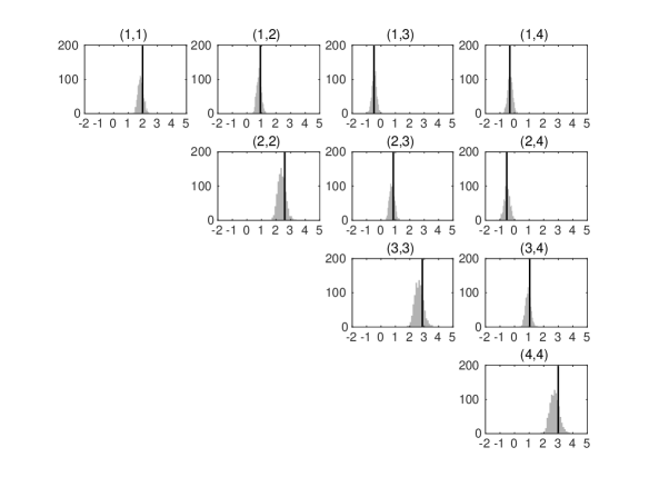
Figure 1: OLS estimates of $\boldsymbol{\Sigma}$ (1)

Note: The shaded areas indicate the histograms of the OLS estimates of $\boldsymbol{\Sigma}$. The vertical lines trace the corresponding true values.

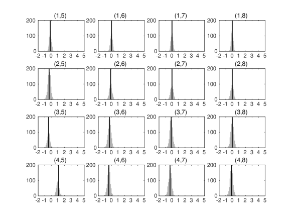
Figure 2: OLS estimates of $\boldsymbol{\Sigma}$ (2)

Note: The shaded areas indicate the histograms of the OLS estimates of $\boldsymbol{\Sigma}$. The vertical lines trace the corresponding true values.

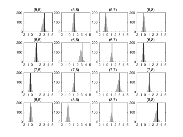
Figure 3: OLS estimates of $\boldsymbol{\Sigma}$ (3)

Note: The shaded areas indicate the histograms of the OLS estimates of $\boldsymbol{\Sigma}$. The vertical lines trace the corresponding true values.

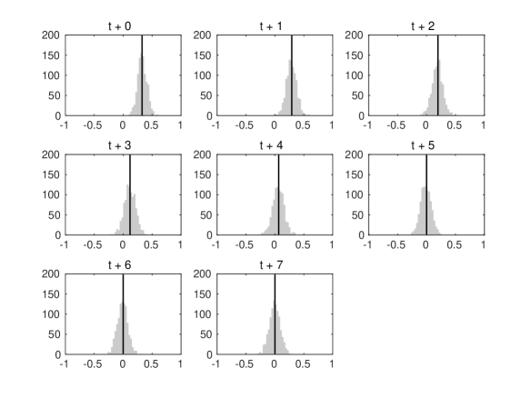
Figure 4: OLS estimates of $\boldsymbol{\gamma}_{IRF}$

Note: The shaded areas indicate the histograms of the OLS estimates of $\boldsymbol{\gamma}_{IRF}$. The vertical lines trace the corresponding true values.

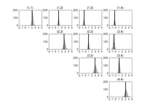
Figure 5: Posterior mean estimates of $\boldsymbol{\Sigma}$ (1)

Note: The shaded areas indicate the histograms of the posterior mean estimates of $\boldsymbol{\Sigma}$. The vertical lines trace the corresponding true values.

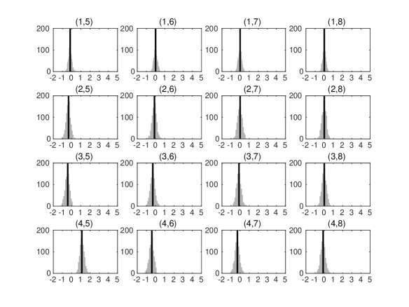
Figure 6: Posterior mean estimates of $\boldsymbol{\Sigma}$ (2)

Note: The shaded areas indicate the histograms of the posterior mean estimates of $\boldsymbol{\Sigma}$. The vertical lines trace the corresponding true values.

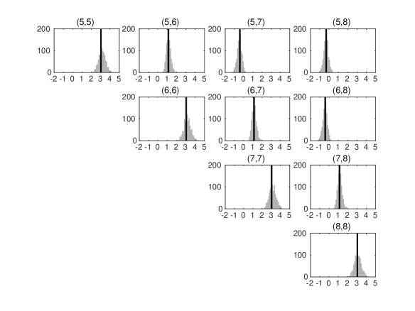
Figure 7: Posterior mean estimates of $\boldsymbol{\Sigma}$ (3)

Note: The shaded areas indicate the histograms of the posterior mean estimates of $\boldsymbol{\Sigma}$. The vertical lines trace the corresponding true values.

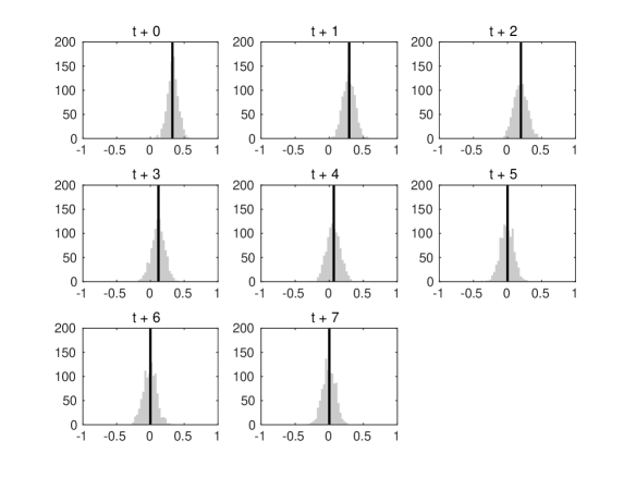
Figure 8: Posterior mean estimates of $\boldsymbol{\gamma}_{IRF}$

Note: The shaded areas indicate the histograms of the posterior mean estimates of $\boldsymbol{\gamma}_{IRF}$. The vertical lines trace the corresponding true values.