Highly accurate special quadrature methods
for Stokesian particle suspensions in confined geometries

Abstract.

Boundary integral methods are highly suited for problems with complicated geometries, but require special quadrature methods to accurately compute the singular and nearly singular layer potentials that appear in them. This paper presents a boundary integral method that can be used to study the motion of rigid particles in three-dimensional periodic Stokes flow with confining walls. A centrepiece of our method is the highly accurate special quadrature method, which is based on a combination of upsampled quadrature and quadrature by expansion (QBX), accelerated using a precomputation scheme. The method is demonstrated for rodlike and spheroidal particles, with the confining geometry given by a pipe or a pair of flat walls. A parameter selection strategy for the special quadrature method is presented and tested. Periodic interactions are computed using the Spectral Ewald (SE) fast summation method, which allows our method to run in $O(n\log n)$ time for $n$ grid points, assuming the number of geometrical objects grows while the grid point concentration is kept fixed.

Keywords: Stokes flow, rigid particle suspensions, boundary integral equations, quadrature by expansion, fast Ewald summation, streamline computation.

Chapter 0 Introduction

Microhydrodynamics is the study of fluid flow at low Reynolds numbers, also known as Stokes flow or creeping flow. Applications are found in biology, for example in the swimming of microorganisms [20] and in blood flow [34], as well as in the field of microfluidics, which concerns the design and construction of miniaturized fluid devices [51]. Suspensions of rigid particles in Stokes flow are important both in various applications and in fundamental fluid mechanics [46, 16, 36, 19]. In this paper, we describe a boundary integral method that can be used to study the motion of rigid particles of different shapes in Stokes flow. The particle suspension may also be confined in a container geometry, such as a pipe or a pair of flat walls. The flow in the fluid domain (i.e. within the container but outside the particles) is governed by the Stokes equations, which for an incompressible Newtonian fluid take the form

$$\nabla p-\mu\nabla^{2}\boldsymbol{u} =\boldsymbol{f},$$ (1)

$$\nabla\cdot\boldsymbol{u} =0.$$ (2)

Here, $p$ is the pressure, $\boldsymbol{u}$ is the flow velocity, $\boldsymbol{f}$ is the body force per unit volume and $\mu$ is the viscosity of the fluid. The Stokes equations arise as a linearization of the Navier–Stokes equations in the case where fluid inertia can be neglected, i.e. when the Reynolds number is much less than 1.

On the surfaces of the particles and walls, no-slip boundary conditions are prescribed. A problem of physical interest is the resistance problem: given the velocities of all particles, compute the forces and torques (caused by viscous resistance) acting on them by the fluid. The inverse problem is called the mobility problem: given the forces and torques acting on all particles by the fluid, compute the particle velocities. The mobility problem is useful in the case of noninertial particles, since then the net force on each particle must be zero, so any external forces (such as gravity) must be balanced by viscous forces from the fluid; given external forces and torques, one can then compute the motion of the particles.

Since the governing equations (1)–(2) are linear, boundary integral methods can be used to solve them. In these methods, the flow is expressed in terms of layer potentials, which are integrals over the boundary of the fluid domain (i.e. over the container walls and particle surfaces). This reduces the dimensionality of the problem from three to two, and leads to a smaller linear system compared to methods that must discretize the whole volume (such as the finite difference or finite element methods). It it also easy to move the particles, since no remeshing is needed. For a detailed discussion on the properties of boundary integral methods, we refer to the books by Pozrikidis [42], Atkinson [1] and Kress [30]. Of special importance are Fredholm integral equations of the second kind, which when discretized, for example using the Nyström method [1, ch. 4][30, sec. 12.2], are known to remain well-conditioned as the system size increases [1, p. 113][30, p. 282].

The linear system resulting from the discretization of a boundary integral equation is dense, and thus naive Gaussian elimination would require $O(N^{3})$ operations to solve a system of $N$ unknowns. Using an iterative solution method such as the generalized minimal residual method (GMRES) [47], the complexity is reduced to $O(N^{2})$ since the condition number and thus the number of iterations are independent of the system size (but may depend on the geometry). For a large system, this complexity is still prohibitive. This can be overcome by using a fast summation method such as the fast multipole method (FMM) [17, 18] or a fast Ewald summation method [13, 32, 27], which reduce the complexity further to $O(N)$ or $O(N\log N)$, respectively.

One of the challenges of boundary integral methods is the need for accurate special quadrature methods for singular and nearly singular integrands. These are necessary when evaluating the layer potentials at a point on the boundary (where the integral kernel is singular) or close to the boundary (where the kernel is nearly singular, i.e. hard to resolve using a quadrature rule designed for smooth integrands). Such special quadrature methods are the main focus of this paper.

1 Overview of related work

In two dimensions, there are excellent special quadrature methods available, such as the one introduced by Helsing and Ojala [21], which has been adapted to simulations of clean [37] and surfactant-covered [39] drops in Stokes flow, as well as vesicles [4]. However, this method is based on a complex variable formulation and not easy to generalize to three dimensions.

In three dimensions, the development of an accurate and efficient special quadrature method is still an active research problem, especially in the nearly singular case. For an overview of methods that have been used, we refer to [29, sec. 1] and [45, sec. 1]. One of the most promising methods which is still under development is quadrature by expansion (QBX), first introduced by Klöckner et al. [29] and Barnett [3] and applied to the Helmholtz equation in two dimensions. This method is based on the observation that the layer potentials are smooth all the way up to the boundary, and can therefore be locally expanded around a point away from the boundary. The expansions can be evaluated at a point closer to the boundary, or even on the boundary itself. The convergence theory of QBX was developed in [14], while [26] analyzed the error from the underlying quadrature rule used to compute the expansion coefficients. A strength of QBX is that it separates source points and target points; the source points enter only in the computation of the expansion coefficients, which can then be used to evaluate the layer potential in all target points within a ball of convergence. QBX has been applied to spheroidal particles in three-dimensional Stokes flow by af Klinteberg and Tornberg [25], using a geometry-specific precomputation scheme to accelerate the computation of the coefficients.

A different approach that has been taken to accelerate QBX is to couple it to a customized FMM, which has been done in two dimensions [43, 44, 58] and more recently in three dimensions [59, 60]. This coupling is a natural step to take since the FMM uses expansions of the same kind as QBX, but it requires nontrivial modifications to the FMM. The resulting method has complexity $O(N)$ and works for any smooth geometry. The work published so far has been for the Laplace and Helmholtz equations, but it is likely to be extended to more kernels, including the ones needed for Stokes flow.

The QBX-FMM methods above all use global QBX, in which all source points are included in forming the local expansion. An alternative is local QBX, in which only source points that are close to the expansion centre are included. Yet another variant is found in [25], where all source points on a single particle is used when forming expansions close to that particle; we call this variant particle-global. Local QBX is typically combined with a patch-based discretization of the geometry. While it reduces the cost of the method, it also poses a challenge since the local layer potential from a single patch may not be as smooth as the global layer potential from the whole geometry (or a whole particle). Different versions of local QBX have been described in two dimensions [3, 43] and three dimensions [49]. The latter paper also uses target-specific expansions, which need only $O(p)$ terms to obtain the same accuracy as a QBX expansion based on spherical harmonics with $O(p^{2})$ terms. However, they sacrifice the separation of source and target that is otherwise present in QBX. This separation is in principle necessary in the QBX-FMM methods, but also in these methods can target-specific expansions be used to lower the computational cost of the method [60].

Some of the recent work have focused on automating the parameter selection based on a given error tolerance, resulting in the adaptive QBX method [28]. The results have so far not been generalized to three dimensions. There has also been work on a kernel-independent version of QBX, called quadrature by kernel-independent expansion (QBKIX) [45] and meant to be combined with the kernel-independent FMM. The published work is in two dimensions, but a generalization to three dimensions is expected to follow.

Other methods, which are not based on QBX, have also been used successfully as special quadrature methods in three dimensions. One example is the “line interpolation method” introduced by Ying et al. [57]. In this method, a line is constructed through the target point, which is close to the boundary, and its projection onto the boundary. The layer potential is evaluated at points further away from the boundary along this line, and also at the projection point where the line intersects the boundary if a separate singular integration method is available. The value at the target point is then computed using interpolation along the line (or extrapolation if no singular integration method is available). Like QBX, the success of this method hinges on the fact that they layer potential is smooth in the domain, so that it can be well interpolated (or extrapolated). It has been applied to surfactant-covered drops [50] and vesicles [35] in three-dimensional Stokes flow. The extrapolatory method used in [34] falls into the same category. Other types of methods are based on regularizing the kernel and adding corrections [5, 53, 6, 54], density interpolation techniques [40], coordinate rotations and a subtraction method [10], asymptotic approximations [11], analytical expressions available only for spheres [12] or floating partitions of unity [9, 61, 23]. Many of these methods are target-specific, and their cost grows rapidly if there are many nearly singular target points.

2 Scope of this paper

In this paper, we present a boundary integral method based on the Stokes double layer potential, which can be used to solve the mobility and resistance problems for a system of rigid particles in incompressible three-dimensional Stokes flow, possibly confined within a container geometry. Our formulation leads to a Fredholm integral equation of the second kind. We use QBX for singular integration, and a combination of QBX and upsampled quadrature for nearly singular integration. Our QBX implementation is based on the work by af Klinteberg and Tornberg [25], which we have extended to rodlike particles, plane walls and pipes (using particle-global QBX for the particles and local QBX for the two wall geometries). A precomputation scheme is used to greatly accelerate the QBX computations for all geometries. For this precomputation scheme to be feasible, we require that each particle or wall is rigid and has some degree of symmetry, such as axisymmetry or reflective symmetry. Nonetheless, we have chosen this route since the implementation is relatively simple compared to e.g. a QBX-FMM method. When container walls are present, we restrict ourselves to periodicity in all three spatial directions and use a fast Ewald summation method called the Spectral Ewald method [31, 23, 24] to accelerate computations. In this situation our method scales as $O(N\log N)$ in the number of unknowns $N$, assuming fixed grid point concentration. The container geometry is restricted to a periodic straight pipe or a pair of periodic plane walls. Our contributions include:

• The combined special quadrature method based on QBX and upsampling, which we have implemented for spheroidal and rodlike particles, plane walls and pipes. (The QBX implementation for spheroids is reused from [25]. Our initial work on QBX for plane walls is published in the conference proceedings [2].)

• A strategy for experimentally selecting the parameters of the special quadrature method to meet a given error tolerance. We also demonstrate that the boundary integral method in full meets the given error tolerance and scales as $O(N\log N)$.

• Construction of fully smooth rodlike particles. We demonstrate the effect of smoothness on the convergence of the local expansions in this particular case.

• Derivation of a stresslet identity for an infinite pipe and a pair of infinite plane walls. This is used as an exact solution to test the special quadrature method.

• An outline of how streamlines can be efficiently computed for periodic problems using the Spectral Ewald method, by reusing data. (This idea was used, but not explicitly described, in [25].)

• The so-called completion sources that appear in our formulation are distributed along the axis of symmetry of rodlike particles, and we have studied how the number of completion sources influences the accuracy.

3 Organization of the paper

In section 1, we introduce the mathematical formulation of the problem, including the boundary integral formulation and the boundary integral equations for the resistance and mobility problems. In section 2, we describe the discretization of the geometry and the quadrature method, including the combined special quadrature. The details on our QBX method are then given in section 3, including the precomputation scheme. In section 4, we describe how periodicity is treated and how the special quadrature is combined with the Spectral Ewald method. Then, in section 5, our parameter selection strategy for the special quadrature is described and demonstrated. Numerical results are given in section 6, to demonstrate the accuracy and scaling of our method. Finally, in section 7, we demonstrate the effect of nonsmooth geometries on the convergence. The appendices include a derivation of the stresslet identity for plane walls and pipes, details on the construction of the smooth rodlike particles, and a note on streamline computation.

Chapter 1 Mathematical formulation

We consider two different kinds of problems: free-space problems and fully periodic problems. In a free-space problem, $M$ particles (spheroids or rods) are located in a fluid extending to infinity. We denote the fluid domain by $\Omega$ and its boundary, i.e. the union of all particle surfaces, by $\Gamma$. The Stokes equations (1)–(2) with $\boldsymbol{f}=\boldsymbol{0}$ hold in $\Omega$, while no-slip boundary conditions are imposed on $\Gamma$. The unit normal vector $\boldsymbol{n}$ of $\Gamma$ is defined to point into the fluid domain $\Omega$, as shown in Figure 1 (a).

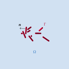
(a) Free-space problem

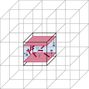
(b) Fully periodic problem

Figure 1: The geometry for (a) a free-space problem, and (b) a fully periodic problem. In (b), the primary cell is marked with a darker outline than the other cells. The geometry is shown only in the primary cell. The lattice of periodic cells fills the whole space; only a small part is shown here.

A fully periodic problem, on the other hand, is periodic in all three spatial directions. The primary cell is a box with side lengths $\boldsymbol{B}=(B_{1},B_{2},B_{3})$, which is considered to be replicated periodically in all three spatial directions, as illustrated by Figure 1 (b). Let the number of particles in the primary cell be $M$. In this case we also allow a container consisting either of a pair of plane walls or a pipe. Only the geometry inside the primary cell is discretized, which means that $\Gamma$ consists of the union of the $M$ particle surfaces and the parts of the wall surfaces that lie in the primary cell. The fluid domain $\Omega$ lies within the container but outside the particles; the flow is thus external to the particles, but internal to the surrounding walls. The unit normal vector $\boldsymbol{n}$ of $\Gamma$ is always defined to point into $\Omega$.

Below, we introduce our boundary integral formulation in the free-space setting, or for the primary cell without periodicity. Full treatment of the periodic problem is deferred to section 4.

1 Boundary integral formulation

Any flow field $\boldsymbol{u}$ that satisfies the Stokes equations (1)–(2) with $\boldsymbol{f}=\boldsymbol{0}$ can be expressed in terms of integrals over the boundary of the fluid domain $\Omega$, as described for example by Pozrikidis [42, ch. 4] and Kim and Karrila [22, ch. 14–16]. The boundary integral formulation that we use is based on the Stokes double layer potential $\boldsymbol{\mathcal{D}}$, which in free space is given by

$$\mathcal{D}_{i}[\Gamma,\boldsymbol{q}](\boldsymbol{x})=\int_{\Gamma}T_{ijk}(\boldsymbol{x}-\boldsymbol{y})q_{j}(\boldsymbol{y})n_{k}(\boldsymbol{y})\,\mathrm{d}S(\boldsymbol{y}),\qquad T_{ijk}(\boldsymbol{r})=-6\frac{r_{i}r_{j}r_{k}}{\lvert\boldsymbol{r}\rvert^{5}}.$$ (1)

Here, $\Gamma$ and $\boldsymbol{n}$ are as in Figure 1, and the double layer density $\boldsymbol{q}$ is a continuous vector field defined on $\Gamma$. The tensor kernel $\boldsymbol{T}$ in (1) is known as the stresslet. The potential $\boldsymbol{\mathcal{D}}$ has a jump discontinuity as $\boldsymbol{x}$ passes over $\Gamma$. More specifically, for $\boldsymbol{x}\in\Gamma$ it holds that [42, p. 110]

$$\lim_{\varepsilon\to 0^{+}}\boldsymbol{\mathcal{D}}[\Gamma,\boldsymbol{q}](\boldsymbol{x}\pm\varepsilon\boldsymbol{n})=\boldsymbol{\mathcal{D}}[\Gamma,\boldsymbol{q}](\boldsymbol{x})\mp 4\pi\boldsymbol{q}(\boldsymbol{x}).$$ (2)

For any closed Lyapunov surface $\tilde{\Gamma}\subseteq\Gamma$ and any constant vector $\tilde{\boldsymbol{q}}$, the stresslet identity [42, p. 28]

$$\boldsymbol{\mathcal{D}}[\tilde{\Gamma},\tilde{\boldsymbol{q}}](\boldsymbol{x})=\begin{cases}\boldsymbol{0},&\text{if $\boldsymbol{x}$ is outside the domain enclosed by $\tilde{\Gamma}$},\\ 4\pi\tilde{\boldsymbol{q}},&\text{if $\boldsymbol{x}\in\tilde{\Gamma}$},\\ 8\pi\tilde{\boldsymbol{q}},&\text{if $\boldsymbol{x}$ is inside the domain enclosed by $\tilde{\Gamma}$},\end{cases}$$ (3)

holds. We will use this identity as a test case for the special quadrature method in sections 5 and 1. In appendix A we show that a variant of (3) holds also for the wall geometries that we consider, despite them not being closed surfaces.

The double layer potential $\boldsymbol{u}(\boldsymbol{x})=\boldsymbol{\mathcal{D}}[\Gamma,\boldsymbol{q}](\boldsymbol{x})$ is a solution to (1)–(2) in $\Omega$ for any continuous vector field $\boldsymbol{q}$. However, not every solution to (1)–(2) can be represented by a double layer potential alone; for instance, as noted in [41][42, p. 119], the force and torque exerted on any particle by the flow from a double layer potential will always be zero, whereas a Stokes flow in general can exert a nonzero force and torque on the particles (which is a central point of the resistance and mobility problems mentioned in section Highly accurate special quadrature methods for Stokesian particle suspensions in confined geometries). This is related to the presence of a nontrivial nullspace of the operator $\boldsymbol{q}\mapsto\boldsymbol{\mathcal{D}}[\Gamma,\boldsymbol{q}]$ for external flows, which can be immediately seen from the stresslet identity (3).

To remove the nontrivial nullspace and allow for nonzero forces and torques on the particles, we add a completion flow $\boldsymbol{\mathcal{V}}$, first introduced by Power and Miranda [41]. The completion flow is also a solution to (1)–(2) and can be identified as the flow from a point force $\boldsymbol{F}$ and a point torque $\boldsymbol{\tau}$ located at $\boldsymbol{y}$. It is given by

$$\mathcal{V}_{i}[\boldsymbol{F},\boldsymbol{\tau},\boldsymbol{y}](\boldsymbol{x})=\frac{1}{8\pi\mu}\left(S_{ij}(\boldsymbol{x}-\boldsymbol{y})F_{j}+R_{ij}(\boldsymbol{x}-\boldsymbol{y})\tau_{j}\right),\qquad\boldsymbol{x}\in\Omega,$$ (4)

where the stokeslet $\boldsymbol{S}$ and the rotlet $\boldsymbol{R}$ are given by

$$S_{ij}(\boldsymbol{r})=\frac{\delta_{ij}}{\lvert\boldsymbol{r}\rvert}+\frac{r_{i}r_{j}}{\lvert\boldsymbol{r}\rvert^{3}}\qquad\text{and}\qquad R_{ij}(\boldsymbol{r})=\epsilon_{ijk}\frac{r_{k}}{\lvert\boldsymbol{r}\rvert^{3}},$$ (5)

respectively. We call a pair $(\boldsymbol{F},\boldsymbol{\tau})$ a completion source. Such completion sources are placed in the interior of every particle. Mathematically, one completion source per particle is sufficient, but this may lead to numerical problems in some cases. In this paper, we allow for multiple completion sources to be distributed along a line segment within the particle; as we show in section 1, this is important for elongated particles. For the particle with index $\alpha$, let $\boldsymbol{F}^{(\alpha)}$ and $\boldsymbol{\tau}^{(\alpha)}$ be the net force and torque, respectively, exerted on the fluid by the particle, and let $\boldsymbol{y}_{\text{c}}^{(\alpha)}$ be the centre of mass of the particle. (For a noninertial particle, $\boldsymbol{F}^{(\alpha)}$ and $\boldsymbol{\tau}^{(\alpha)}$ would be equal to the net external force and torque, respectively, acting on the particle.) The completion flow associated with particle $\alpha$ is then given by

$$\boldsymbol{\mathcal{V}}^{(\alpha)}[\boldsymbol{F}^{(\alpha)},\boldsymbol{\tau}^{(\alpha)}](\boldsymbol{x})=\frac{1}{N_{\text{src}}}\sum_{s=1}^{N_{\text{src}}}\boldsymbol{\mathcal{V}}[\boldsymbol{F}^{(\alpha)},\boldsymbol{\tau}^{(\alpha)},\boldsymbol{y}_{\text{c}}^{(\alpha)}+C(s,N_{\text{src}})\boldsymbol{a}^{(\alpha)}](\boldsymbol{x}),$$ (6)

where $N_{\text{src}}$ is the number of completion sources per particle, $\boldsymbol{\mathcal{V}}$ is given by (4), and $\boldsymbol{a}^{(\alpha)}$ is a vector specifying the line segment along which completion sources are placed. The function $C$ is given by

$$C(s,N_{\text{src}})=\begin{cases}0,&\text{if $N_{\text{src}}=1$},\\ -1+2\dfrac{s-1}{N_{\text{src}}-1},&\text{if $N_{\text{src}}>1$}.\end{cases}$$ (7)

Both the double layer potential $\boldsymbol{\mathcal{D}}$ and the completion flow $\boldsymbol{\mathcal{V}}$ have the property that they decay to zero as $\boldsymbol{x}\to\infty$. To be able to represent flows which do not decay, we add a background flow $\boldsymbol{u}_{\text{bg}}$, which is a known solution to (1)–(2) in the whole physical space, ignoring all particles and walls. The total flow $\boldsymbol{u}$ in the presence of particles and walls is thus written as

$$\boldsymbol{u}(\boldsymbol{x})=\boldsymbol{u}_{\text{bg}}(\boldsymbol{x})+\boldsymbol{u}_{\text{d}}(\boldsymbol{x}),$$ (8)

where $\boldsymbol{u}_{\text{d}}$ is a disturbance flow which is responsible for enforcing the no-slip boundary conditions on the solid boundary $\Gamma$. As $\boldsymbol{x}$ moves away from $\Gamma$, the disturbance flow $\boldsymbol{u}_{\text{d}}$ should decay to zero, and the total flow should therefore approach the background flow $\boldsymbol{u}_{\text{bg}}$. The disturbance flow is written as

$$\boldsymbol{u}_{\text{d}}(\boldsymbol{x})=\boldsymbol{\mathcal{D}}[\Gamma,\boldsymbol{q}](\boldsymbol{x})+\sum_{\alpha=1}^{M}\boldsymbol{\mathcal{V}}^{(\alpha)}[\boldsymbol{F}^{(\alpha)},\boldsymbol{\tau}^{(\alpha)}](\boldsymbol{x}),$$ (9)

where $\boldsymbol{\mathcal{V}}^{(\alpha)}$ is as in (6), and the double layer density $\boldsymbol{q}$ must be determined through the boundary conditions. Note that $\boldsymbol{u}_{\text{d}}$ as given by (9) decays as $\boldsymbol{x}\to\infty$, and by the superposition principle it satisfies (1)–(2). Also note that completion sources are placed inside the particles since the flow is external to the particles, but not inside the walls since the flow is internal to the walls (for details we refer to [42, sec. 4.5]). On the other hand, the double layer density $\boldsymbol{q}$ is defined on the surfaces of both the particles and walls. The formulation (9) is complete, meaning that any flow which satisfies (1)–(2) and decays as $\boldsymbol{x}\to\infty$ can be represented in this way.

To derive the fundamental boundary integral equation, which is used to determine the double layer density $\boldsymbol{q}$ in (9), we insert (9) into (8) and then let $\boldsymbol{x}\in\Omega$ approach the solid boundary $\Gamma$. Enforcing no-slip boundary conditions on $\Gamma$ yields, recalling the jump condition (2),

$$\boldsymbol{u}(\boldsymbol{x})=\boldsymbol{u}_{\text{bg}}(\boldsymbol{x})+\boldsymbol{\mathcal{D}}[\Gamma,\boldsymbol{q}](\boldsymbol{x})-4\pi\boldsymbol{q}(\boldsymbol{x})+\sum_{\alpha=1}^{M}\boldsymbol{\mathcal{V}}^{(\alpha)}[\boldsymbol{F}^{(\alpha)},\boldsymbol{\tau}^{(\alpha)}](\boldsymbol{x})=\boldsymbol{U}_{\Gamma}(\boldsymbol{x}),\qquad\boldsymbol{x}\in\Gamma.$$ (10)

The presence of the term $-4\pi\boldsymbol{q}(\boldsymbol{x})$, which is due to the jump condition, makes the boundary integral equation (10) a Fredholm integral equation of the second kind. The right-hand side $\boldsymbol{U}_{\Gamma}$ is the pointwise velocity of the boundary $\Gamma$. We assume the walls to be stationary and the particles to move as rigid bodies. This means that, if we let $\Gamma_{\text{w}}$ be the union of all wall surfaces and $\Gamma_{\text{p}}^{(\alpha)}$ the surface of particle $\alpha$,

$$\boldsymbol{U}_{\Gamma}(\boldsymbol{x})=\begin{cases}\boldsymbol{0},&\boldsymbol{x}\in\Gamma_{\text{w}},\\ \boldsymbol{U}_{\text{RBM}}^{(\alpha)}+\boldsymbol{\Omega}_{\text{RBM}}^{(\alpha)}\times(\boldsymbol{x}-\boldsymbol{y}_{\text{c}}^{(\alpha)}),&\boldsymbol{x}\in\Gamma_{\text{p}}^{(\alpha)},\end{cases}$$ (11)

where $\boldsymbol{U}_{\text{RBM}}^{(\alpha)}$ and $\boldsymbol{\Omega}_{\text{RBM}}^{(\alpha)}$ are the translational and angular velocity, respectively, of particle $\alpha$ (with RBM denoting rigid body motion).

As mentioned in section Highly accurate special quadrature methods for Stokesian particle suspensions in confined geometries, the viscous resistance that the particles experience from the fluid is related to their velocities. In the resistance problem, the velocities (i.e. $\boldsymbol{U}_{\text{RBM}}^{(\alpha)}$ and $\boldsymbol{\Omega}_{\text{RBM}}^{(\alpha)}$ for each particle) are specified in (10)–(11), while in the mobility problem, the viscous forces and torques (i.e. $\boldsymbol{F}^{(\alpha)}$ and $\boldsymbol{\tau}^{(\alpha)}$ for each particle) are specified [42, p. 129]. The boundary integral equations resulting from these two problems are described in more detail below. In both cases, the resulting integral equation is discretized using the Nyström method, as described in section 2.

1 The resistance problem

In this case, the velocities $\boldsymbol{U}_{\text{RBM}}^{(\alpha)}$ and $\boldsymbol{\Omega}_{\text{RBM}}^{(\alpha)}$ of all particles are known, while the corresponding forces $\boldsymbol{F}^{(\alpha)}$ and torques $\boldsymbol{\tau}^{(\alpha)}$ are to be computed. Following [42, p. 130], the forces and torques are related to the unknown double layer density $\boldsymbol{q}$ by stipulating

$$\boldsymbol{F}^{(\alpha)}[\boldsymbol{q}]=\int_{\Gamma_{\text{p}}^{(\alpha)}}\boldsymbol{q}(\boldsymbol{y})\,\mathrm{d}S_{\boldsymbol{y}}\qquad\text{and}\qquad\boldsymbol{\tau}^{(\alpha)}[\boldsymbol{q}]=\int_{\Gamma_{\text{p}}^{(\alpha)}}(\boldsymbol{y}-\boldsymbol{y}_{\text{c}}^{(\alpha)})\times\boldsymbol{q}(\boldsymbol{y})\,\mathrm{d}S_{\boldsymbol{y}}.$$ (12)

These relations are inserted into (10), which can then be rearranged as

$$\boldsymbol{\mathcal{D}}[\Gamma,\boldsymbol{q}](\boldsymbol{x})-4\pi\boldsymbol{q}(\boldsymbol{x})+\sum_{\alpha=1}^{M}\boldsymbol{\mathcal{V}}^{(\alpha)}[\boldsymbol{F}^{(\alpha)}[\boldsymbol{q}],\boldsymbol{\tau}^{(\alpha)}[\boldsymbol{q}]](\boldsymbol{x})=\boldsymbol{U}_{\Gamma}(\boldsymbol{x})-\boldsymbol{u}_{\text{bg}}(\boldsymbol{x}),\qquad\boldsymbol{x}\in\Gamma.$$ (13)

After solving this integral equation for $\boldsymbol{q}$, the forces and torques can be computed using (12), and the flow field can then be computed using (8)–(9).

2 The mobility problem

In this case, the force $\boldsymbol{F}^{(\alpha)}$ and torque $\boldsymbol{\tau}^{(\alpha)}$ exerted on the fluid by each particle (which for a noninertial particle are equal to the net external force and torque acting on the particle) are known, but not the particle velocities $\boldsymbol{U}_{\text{RBM}}^{(\alpha)}$ and $\boldsymbol{\Omega}_{\text{RBM}}^{(\alpha)}$. Following [42, p. 135], the velocities are related to the double layer density $\boldsymbol{q}$ by

$$\boldsymbol{U}_{\text{RBM}}^{(\alpha)}[\boldsymbol{q}] =-\frac{4\pi}{\lvert\Gamma_{\text{p}}^{(\alpha)}\rvert}\int_{\Gamma_{\text{p}}^{(\alpha)}}\boldsymbol{q}(\boldsymbol{y})\,\mathrm{d}S_{\boldsymbol{y}},$$ (14)

$$\boldsymbol{\Omega}_{\text{RBM}}^{(\alpha)}[\boldsymbol{q}] =-4\pi\sum_{n=1}^{3}\frac{\boldsymbol{\omega}_{n}^{(\alpha)}}{A_{n}^{(\alpha)}}\,\bigg{(}\boldsymbol{\omega}_{n}^{(\alpha)}\cdot\int_{\Gamma_{\text{p}}^{(\alpha)}}(\boldsymbol{y}-\boldsymbol{y}_{\text{c}}^{(\alpha)})\times\boldsymbol{q}(\boldsymbol{y})\,\mathrm{d}S_{\boldsymbol{y}}\bigg{)}.$$ (15)

Here, $\lvert\Gamma_{\text{p}}^{(\alpha)}\rvert$ is the surface area of $\Gamma_{\text{p}}^{(\alpha)}$, and

$$A_{n}^{(\alpha)}=\int_{\Gamma_{\text{p}}^{(\alpha)}}\left\lvert\boldsymbol{\omega}_{n}^{(\alpha)}\times(\boldsymbol{y}-\boldsymbol{y}_{\text{c}}^{(\alpha)})\right\rvert^{2}\,\mathrm{d}S_{\boldsymbol{y}},$$ (16)

while $\boldsymbol{\omega}_{n}^{(\alpha)}$ are three linearly independent unit vectors which must satisfy

$$\frac{1}{\sqrt{A_{m}^{(\alpha)}A_{n}^{(\alpha)}}}\int_{\Gamma_{\text{p}}^{(\alpha)}}\!\left[\boldsymbol{\omega}_{m}^{(\alpha)}\times(\boldsymbol{y}-\boldsymbol{y}_{\text{c}}^{(\alpha)})\right]\cdot\!\left[\boldsymbol{\omega}_{n}^{(\alpha)}\times(\boldsymbol{y}-\boldsymbol{y}_{\text{c}}^{(\alpha)})\right]\,\mathrm{d}S_{\boldsymbol{y}}=\delta_{mn},\qquad m,n=1,2,3.$$ (17)

The boundary integral equation (10) can then be rearranged as

$$\boldsymbol{\mathcal{D}}[\Gamma,\boldsymbol{q}](\boldsymbol{x})-4\pi\boldsymbol{q}(\boldsymbol{x})-\boldsymbol{U}_{\Gamma}[\boldsymbol{q}](\boldsymbol{x})=-\boldsymbol{u}_{\text{bg}}(\boldsymbol{x})-\sum_{\alpha=1}^{M}\boldsymbol{\mathcal{V}}^{(\alpha)}[\boldsymbol{F}^{(\alpha)},\boldsymbol{\tau}^{(\alpha)}](\boldsymbol{x}),\qquad\boldsymbol{x}\in\Gamma,$$ (18)

where $\boldsymbol{U}_{\Gamma}[\boldsymbol{q}]$ is given by (11) but with $\boldsymbol{U}_{\text{RBM}}^{(\alpha)}$ and $\boldsymbol{\Omega}_{\text{RBM}}^{(\alpha)}$ replaced by the expressions in (14) and (15), respectively. After solving (18) for $\boldsymbol{q}$, the velocities can be computed using (14)–(15), and the flow field can be computed using (8)–(9).

Chapter 2 Discretization and quadrature

In order to solve the boundary integral equation (13) associated with the resistance problem, or the boundary integral equation (18) associated with the mobility problem, the integral operators in these equations must be discretized. This amounts to discretizing the double layer potential $\boldsymbol{\mathcal{D}}$, as well as the integrals occurring in relation (12) for the resistance problem, or relation (14)–(15) for the mobility problem. Following [25], we introduce the notation

$$\mathrm{I}[f]=\int_{\Gamma}f(\boldsymbol{y})\,\mathrm{d}S(\boldsymbol{y})$$ (1)

for the integral of the arbitrary function $f$ over the surface $\Gamma$. We introduce a quadrature rule $Q_{N}$ called the direct quadrature rule, defined by a set of $N$ nodes $\boldsymbol{x}_{i}\in\Gamma$ and weights $w_{i}\in\mathbb{R}$, $i=1,\ldots,N$. The details of this quadrature rule is specified in sections 1 and 2. Using the direct quadrature rule $Q_{N}$, the integral in (1) can be approximated as

$$\mathrm{I}[f]\approx Q_{N}[f]=\sum_{i=1}^{N}f(\boldsymbol{x}_{i})w_{i}.$$ (2)

We denote an integral quantity approximated by $Q_{N}$ with a superscript $h$, for example the double layer potential

$$\mathcal{D}^{h}_{i}[\Gamma,\boldsymbol{q}](\boldsymbol{x})=Q_{N}[T_{ijk}(\boldsymbol{x}-{\cdot})q_{j}(\cdot)n_{k}(\cdot)].$$ (3)

We then discretize (13) or (18) using the Nyström method [1, ch. 4][30, sec. 12.2], in which the integral equation is enforced in the quadrature nodes. For the resistance problem, (13) then becomes

$$\boldsymbol{\mathcal{D}}^{h}[\Gamma,\boldsymbol{q}](\boldsymbol{x}_{i})-4\pi\boldsymbol{q}(\boldsymbol{x}_{i})+\sum_{\alpha=1}^{M}\boldsymbol{\mathcal{V}}^{(\alpha),h}[\boldsymbol{F}^{(\alpha)}[\boldsymbol{q}],\boldsymbol{\tau}^{(\alpha)}[\boldsymbol{q}]](\boldsymbol{x}_{i})=\boldsymbol{U}_{\Gamma}(\boldsymbol{x}_{i})-\boldsymbol{u}_{\text{bg}}(\boldsymbol{x}_{i}),\qquad i=1,\ldots,N.$$ (4)

For the mobility problem, (18) becomes

$$\boldsymbol{\mathcal{D}}^{h}[\Gamma,\boldsymbol{q}](\boldsymbol{x}_{i})-4\pi\boldsymbol{q}(\boldsymbol{x}_{i})-\boldsymbol{U}^{h}_{\Gamma}[\boldsymbol{q}](\boldsymbol{x}_{i})=-\boldsymbol{u}_{\text{bg}}(\boldsymbol{x}_{i})-\sum_{\alpha=1}^{M}\boldsymbol{\mathcal{V}}^{(\alpha)}[\boldsymbol{F}^{(\alpha)},\boldsymbol{\tau}^{(\alpha)}](\boldsymbol{x}_{i}),\qquad i=1,\ldots,N.$$ (5)

The superscript $h$ on $\boldsymbol{\mathcal{V}}^{(\alpha),h}$ in (4) and $\boldsymbol{U}_{\Gamma}^{h}$ in (5) signifies that these quantities, while not integrals themselves, contain integrals – namely (12) or (14)–(15) – which are approximated using the direct quadrature rule $Q_{N}$. In both cases, the resulting linear system is solved iteratively using the generalized minimal residual method (GMRES).

In this paper, we consider two distinct types of geometrical objects, namely particles and walls, as indicated by Figure 1. Particles are mobile rigid bodies immersed in the fluid, while walls are stationary and surround the fluid domain. We consider two types of particles: spheroids, which are given by a surface

$$\frac{x_{1}^{2}+x_{2}^{2}}{a^{2}}+\frac{x_{3}^{2}}{c^{2}}=1$$ (6)

in local coordinates; and rods, which consist of a cylinder with rounded caps, described in appendix B. We also consider two types of walls, namely plane walls and pipes with circular cross section. Both wall geometries extend to infinity in the periodic setting, but we discretize only the part of each object that lies inside the primary cell.

Figure 1: The geometrical objects considered in this paper are (a) particles (spheroids and rods) and (b) walls (plane walls and pipes). The quadrature rule is different for particles and walls.

The nature of the direct quadrature rule $Q_{N}$ is different for particles and walls: for particles, it is a particle-global quadrature rule described in section 1, while for walls it is a local patch-based quadrature rule described in section 2. The special quadrature method for particles and walls is introduced in section 3.

It should be noted that all geometrical objects shown in Figure 1 are smooth, i.e. of class $C^{\infty}$. The construction of the smooth rod particles is described in appendix B. In section 7, we consider the effect that a nonsmooth object would have on the convergence of the special quadrature method.

1 Direct quadrature for particles

The discretization and direct quadrature rule of the spheroids are exactly the same as in [25], while for the rods they are a slight variation of the former. Both kinds of particles are axisymmetric, and their parametrizations take this into account, with one parameter $\varphi\in[0,2\pi)$ varying in the azimuthal direction and the other parameter $\theta\in[0,\pi]$ varying in the polar direction. For instance, the spheroid (6) is parametrized using spherical coordinates as

$$\begin{cases}x_{1}=a\sin\theta\cos\varphi,\\ x_{2}=a\sin\theta\sin\varphi,\\ x_{3}=c\cos\theta.\end{cases}$$ (7)

It is discretized using a tensorial grid with $n_{\theta}\times n_{\varphi}$ grid points. For the polar direction, let $(\theta_{i},\lambda^{\theta}_{i})$, $i=1,\ldots,n_{\theta}$, be the nodes and weights of an $n_{\theta}$-point Gauss–Legendre quadrature rule [38, sec. 3.5(v)] on the interval $[0,\pi]$. For the azimuthal direction, let $(\varphi_{j},\lambda^{\varphi}_{j})$, $j=1,\ldots,n_{\varphi}$, be the nodes and weights of the trapezoidal rule on the interval $[0,2\pi)$. Since the integrand is periodic on this interval, the trapezoidal rule has spectral accuracy in this case [56]. The resulting tensorial quadrature rule, called the direct quadrature rule of the spheroid, is

$$Q_{n_{\theta}n_{\varphi}}[f]=\sum_{i=1}^{n_{\theta}}\sum_{j=1}^{n_{\varphi}}f(\boldsymbol{x}(\theta_{i},\varphi_{j}))W_{\text{sph}}(\theta_{i},\varphi_{j})\lambda_{i}^{\theta}\lambda_{j}^{\varphi},$$ (8)

where $W_{\text{sph}}(\theta,\varphi)$ is the area element associated with the parametrization (7).

The rod consists of a cylinder with rounded caps. While the surface is smooth everywhere, the grid is divided into three parts as shown in Figure 2. The reason for this is to be able to increase the resolution at the caps independently of the resolution at the middle of the rod.

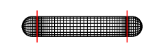
Figure 2: The grid on the rods consists of three parts: two caps and a middle cylinder.

The rod is parametrized as

$$\begin{cases}x_{1}=\varrho(\theta;L,R)\cos\varphi,\\ x_{2}=\varrho(\theta;L,R)\sin\varphi,\\ x_{3}=\beta(\theta;L,R),\end{cases}$$ (9)

where $L$ is the length of the rod and $R$ its radius. The shape functions $\varrho(\cdot\,;L,R):[0,\pi]\to[0,R]$ and $\beta(\cdot\,;L,R):[0,\pi]\to[-\tfrac{1}{2}L,\tfrac{1}{2}L]$ are described in appendix B. They are chosen such that $\theta\in[0,\pi/3]=I_{1}$ and $\theta\in[2\pi/3,\pi]=I_{3}$ correspond to the two caps, while $\theta\in[\pi/3,2\pi/3]=I_{2}$ corresponds to the middle part. Each cap is discretized using $n_{1}\times n_{\varphi}$ grid points, and the middle cylinder is discretized using $n_{2}\times n_{\varphi}$ grid points, so the total grid has $(2n_{1}+n_{2})\times n_{\varphi}$ grid points. The trapezoidal rule is again used in the azimuthal direction. In the polar direction, a separate Gauss–Legendre quadrature rule is used for each of the three parts. The tensorial direct quadrature rule of the rod is thus (with $n_{3}=n_{1}$)

$$Q_{(2n_{1}+n_{2})n_{\varphi}}[f]=\sum_{k=1}^{3}\sum_{i=1}^{n_{k}}\sum_{j=1}^{n_{\varphi}}f(\boldsymbol{x}(\theta_{i}^{k},\varphi_{j}))W_{\text{rod}}(\theta_{i}^{k},\varphi_{j})\lambda_{i}^{k}\lambda_{j}^{\varphi},$$ (10)

where $(\theta^{k}_{i},\lambda^{k}_{i})$, $i=1,\ldots,n_{k}$, are the nodes and weights of an $n_{k}$-point Gauss–Legendre quadrature on the interval $I_{k}$, and $W_{\text{rod}}(\theta,\varphi)$ is the area element associated with (9).

The direct quadrature rules (8) and (10) are both particle-global in the sense that each particle is treated as a single unit, and the quadrature rule is applied to the particle as a whole. The quadrature rules has spectral accuracy for smooth integrands, i.e. it converges exponentially as the number of grid points increases.

2 Direct quadrature for walls

The wall geometries are present only in the periodic setting, and then only the part inside the primary cell needs to be discretized. For the plane wall, this part consists of a flat rectangle of size $L_{1}\times L_{2}$, which is divided into $P_{1}\times P_{2}$ flat subrectangles, called patches. Each patch is discretized using a tensorial grid with $n_{1}\times n_{2}$ Gauss–Legendre grid points, as shown in Figure 3 (a). In each direction of the patch, an $n_{d}$-point Gauss–Legendre quadrature rule is used with nodes and weights $(s_{i}^{d},\lambda_{i}^{d})$, $i=1,\ldots,n_{d}$, $d=1,2$. The resulting tensorial direct quadrature rule of the patch is

$$Q_{n_{1}n_{2}}[f]=\sum_{i=1}^{n_{1}}\sum_{j=1}^{n_{2}}f(\boldsymbol{x}(s_{i}^{1},s_{j}^{2}))W_{\text{wall}}(s_{i}^{1},s_{j}^{2})\lambda_{i}^{1}\lambda_{j}^{2},$$ (11)

where $W_{\text{wall}}(s^{1},s^{2})$ is the area element of the wall.

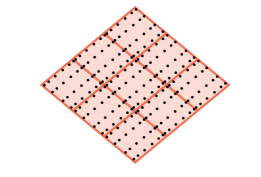
(a) Plane wall

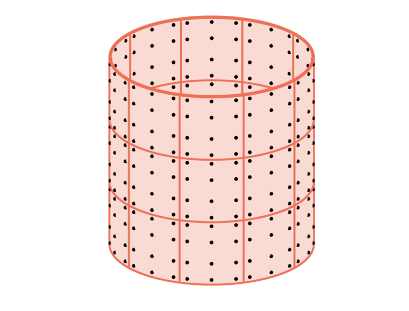
(b) Pipe

Figure 3: (a) A plane wall divided into $3\times 3$ patches, each patch discretized using $6\times 4$ grid points. (b) A pipe divided into $3\times 10$ patches, each patch discretized using $4\times 3$ grid points.

The part of the pipe in the primary cell consists of a cylinder with radius $R_{\text{c}}$ and length $L_{\text{c}}$. Like the plane wall, it is divided into rectangular patches, but these are curved, as seen in Figure 3 (b). Apart from that, the discretization and quadrature rule are the same as for the plane wall. The direct quadrature rule of the pipe is thus also given by (11), the only difference compared to the plane wall being the area element $W_{\text{wall}}$ and the parametrization $(s^{1},s^{2})\mapsto\boldsymbol{x}$.

The direct quadrature rule (11) is local in the sense that the wall is subdivided into smaller patches, and the quadrature rule is applied to each patch separately. The grid can be refined in two different ways: by adding more grid points to each patch (which we call $n$-refinement), or by reducing the size of the patches and thus increasing their number (which we call $P$-refinement). Under $n$-refinement, the quadrature rule has spectral accuracy like the direct quadrature rule of the particles, while under $P$-refinement the quadrature rule is polynomially accurate with order determined by $n_{1}$ and $n_{2}$.

3 Special quadrature: upsampled quadrature and quadrature by expansion (QBX)

The double layer potential $\boldsymbol{\mathcal{D}}$ given by (1) is challenging to compute using direct quadrature in two different situations, in both cases due to its kernel $\boldsymbol{T}$. Firstly, when the evaluation point $\boldsymbol{x}$ is on $\Gamma$ itself, $\boldsymbol{T}$ becomes singular at the point $\boldsymbol{y}=\boldsymbol{x}$ (we refer to this as the singular case or the onsurface evaluation case). The integral exists as an improper integral as long as $\Gamma$ is a Lyapunov surface [42, p. 37], but clearly a special quadrature method of some sort is needed to compute it. Secondly, when $\boldsymbol{x}\in\Omega$ is close to $\Gamma$, but not on $\Gamma$, $\boldsymbol{T}$ becomes very peaked and thus hard to resolve using the direct quadrature rule (we refer to this as the nearly singular case or the offsurface evaluation case).

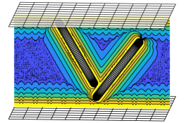
(a) Direct quadrature error

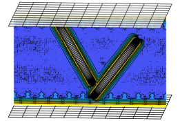
(b) Upsampled quadrature error, $\kappa=2$

(c)

Figure 4: Relative error in the centre plane when evaluating the stresslet identity (3) for two rod particles between a pair of parallel horizontal plane walls in a periodic setting, using the direct quadrature rule in (a) and the upsampled quadrature rule with upsampling factor $\kappa=2$ in (b). Note that the error is still large very close to the particles and walls in (b). The density $\boldsymbol{q}$ is constant in this example, so the error in (a) and (b) comes entirely from the nearly singular behaviour of the stresslet $\boldsymbol{T}$.

The singular case is always present when solving the boundary integral equation (10), while the nearly singular case occurs when particles are close to each other or close to a wall, and also if the flow field (8)–(9) is to be computed close to a particle or wall. The latter situation is illustrated in Figure 4 (a), where the error grows exponentially as the evaluation point $\boldsymbol{x}$ approaches the boundary $\Gamma$. This behaviour is well-known, and in two dimensions there are error estimates available for the Laplace and Helmholtz potentials in [26] and for the Stokes potential in [39]. To compute the double layer potential accurately close to a particle or wall, special quadrature is needed. Here, we consider two types of special quadrature: upsampled quadrature and quadrature by expansion (QBX).

Assuming that the density $\boldsymbol{q}$ itself is well-resolved on the grid, upsampled quadrature provides a partial solution for the nearly singular case. In upsampled quadrature, the double layer density $\boldsymbol{q}$ is interpolated onto a grid refined by a factor $\kappa$ in both directions, and the integral is then evaluated using direct quadrature on the finer grid. For the particle-global quadrature rules in section 1, the grid of the whole particle is refined (increasing the number of grid points of each individual quadrature rule). The density is interpolated onto the finer grid using trigonometric interpolation in the azimuthal direction and barycentric Lagrange interpolation [7] in the polar direction. For the local patch-based quadrature rules in section 2, only the $N_{\text{P}}$ patches closest to the evaluation point $\boldsymbol{x}$ are refined, using $n$-refinement (thus increasing the number of grid points on them); other patches are sufficiently far away from the singularity that direct quadrature can be used. This is illustrated in Figure 5 for $N_{\text{P}}=9$. The refinement has spectral accuracy for both particles and walls. Since all geometrical objects are rigid, interpolation matrices can be precomputed.

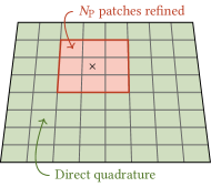
Figure 5: Upsampled quadrature for a plane wall: the $N_{\text{P}}$ patches closest to the evaluation point (marked with $\times$) are refined, here for $N_{\text{P}}=9$. The other patches are treated using direct quadrature without refinement.

As Figure 4 (b) shows, upsampled quadrature pushes the region where the error is large closer to the boundary $\Gamma$. However, the error will always be large very close to $\Gamma$ no matter how large the upsampling factor $\kappa$ is. To be able to achieve small errors arbitrarily close to $\Gamma$, we use a special quadrature rule specifically designed for layer potentials with singular kernels, namely quadrature by expansion (QBX) [29, 3]. The idea behind QBX is to make a local series expansion of the potential $\boldsymbol{\mathcal{D}}$ in the fluid domain, which converges rapidly since $\boldsymbol{\mathcal{D}}$ is smooth all the way up to the boundary $\Gamma$. The expansion is made around a point $\boldsymbol{c}$, called the expansion centre, which is inside the fluid domain (i.e. not on $\Gamma$), and it can be used to evaluate the potential inside a ball around $\boldsymbol{c}$ called the ball of convergence, as shown in Figure 6. The expansion is valid even at the point where the ball touches $\Gamma$ [14], and can therefore be used in the singular case as well as the nearly singular case. The application of QBX to the Stokes double layer potential $\boldsymbol{\mathcal{D}}$ will be described in detail in section 3.

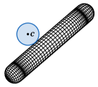
(a)

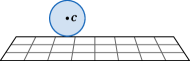
(b)

Figure 6: The idea behind QBX is to make a series expansion of the potential close to a particle (a) or wall (b), valid inside a ball of convergence shown as a blue disc. The expansion is also valid at the point where the ball of convergence touches the boundary.

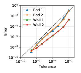
(a) Layer density error

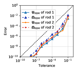
(b) Particle velocity error

Figure 7: (a) Maximal absolute error of the layer density on each geometrical object (colors as in Figure 6 (a)), estimated using a reference solution with tolerance ${10}^{-9}$. (b) Absolute error of the particle velocities.

In this paper, we use a combined quadrature strategy, where direct quadrature is used far away from the boundary, upsampled quadrature is used in an intermediate region, and QBX is used in a small region closest to the boundary, as illustrated in Figure 7. For each particle and wall in the geometry, the evaluation point $\boldsymbol{x}$ is classified into one of these three regions, and the contribution to the double layer potential $\boldsymbol{\mathcal{D}}$ from that particle or wall is computed as follows:

• If $\boldsymbol{x}$ is in the direct quadrature region, the double layer potential (1) is computed using direct quadrature (3) over the whole particle or wall, as described in sections 1 and 2.

• If $\boldsymbol{x}$ is in the upsampled quadrature region, the behaviour is different for particles and walls, as described above. For a particle, the density is upsampled globally on the whole particle surface and then integrated using direct quadrature on the fine grid. For a wall, the density is upsampled only on the $N_{\text{P}}$ patches closest to the evaluation point, while direct quadrature without upsampling is used on the other patches (as in Figure 5).

• If $\boldsymbol{x}$ is in the QBX region, the behaviour is similar to the upsampled quadrature region. For a particle, the density on the whole particle surface is used when computing the coefficients of the local expansion which is then used at the evaluation point (particle-global QBX). For a wall, only the density on the $N_{\text{P}}$ patches closest to the expansion centre $\boldsymbol{c}$ is used to compute the expansion (local QBX), while the contribution from other patches is computed using direct quadrature. In other words, the expansion is computed using a truncated wall, with $N_{\text{P}}$ determining the number of patches in the truncated wall. The difference between particle-global and local QBX is described in more detail in section 2.

The total double layer potential at $\boldsymbol{x}$ is then retrieved using superposition, i.e. by summing the contributions from all particles and walls.

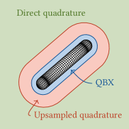
(a)

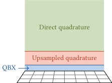
(b)

Figure 7: The regions of the combined quadrature strategy, shown here for a rod particle in (a) and a plane wall in (b). Depending on the location of the evaluation point $\boldsymbol{x}$, it is treated using direct quadrature, upsampled quadrature or QBX.

When using local QBX, the convergence rate of the local expansion will depend on the ratio between the distance from $\boldsymbol{c}$ to the wall and the distance from $\boldsymbol{c}$ to the edge of the truncated wall [49]. We have observed that $N_{\text{P}}=1$ is too low for the wall QBX region in our case, since the expansion centre may then be too close to the edge of the truncated wall. Setting $N_{\text{P}}=9$ seems to be sufficient to remedy this, and increasing $N_{\text{P}}$ further has no effect. We therefore fix $N_{\text{P}}=9$ both for the QBX region and the upsampled quadrature region of plane walls and pipes, for the rest of this paper.

The distances from the surface at which to switch from one quadrature region to the next (i.e. direct quadrature, upsampled quadrature, QBX) are parameters to be set, and these will be discussed in section 5.

Chapter 3 Quadrature by expansion for the Stokes double layer potential

In order to apply QBX to the Stokes double layer potential $\boldsymbol{\mathcal{D}}$ given by (1), we need to be able to write down a local expansion of the potential. We use the same approach as in [25], which is summarized in section 1. The differences between particles (for which particle-global QBX is used) and walls (for which local QBX is used) are summarized in section 2. Finally, the precomputation scheme which is crucial for accelerating the method is described in section 3.

1 Local expansion of the double layer potential

Instead of expanding the double layer potential $\boldsymbol{\mathcal{D}}$ itself directly, we use the fact that $\boldsymbol{\mathcal{D}}$ can be expressed in terms of the so-called dipole potential $\mathcal{L}$ using the relation [55, 25]

$$\mathcal{D}_{i}[\tilde{\Gamma},\boldsymbol{q}](\boldsymbol{x})=\left(x_{j}\frac{\mathrm{\partial}}{\mathrm{\partial}x_{i}}-\delta_{ij}\right)\mathcal{L}[\tilde{\Gamma},q_{j}\boldsymbol{n}+n_{j}\boldsymbol{q}](\boldsymbol{x})-\frac{\mathrm{\partial}}{\mathrm{\partial}x_{i}}\mathcal{L}[\tilde{\Gamma},y_{k}q_{k}\boldsymbol{n}+y_{k}n_{k}\boldsymbol{q}](\boldsymbol{x}),$$ (1)

where $\tilde{\Gamma}$ is any subset of $\Gamma$. The dipole potential is the double layer potential of the Laplace equation and is defined as

$$\mathcal{L}[\tilde{\Gamma},\boldsymbol{\rho}](\boldsymbol{x})=\int_{\tilde{\Gamma}}\boldsymbol{\rho}(\boldsymbol{y})\cdot\nabla_{\boldsymbol{y}}\frac{1}{\lvert\boldsymbol{x}-\boldsymbol{y}\rvert}\,\mathrm{d}S(\boldsymbol{y}).$$ (2)

The kernel of the dipole potential has a natural expansion based on the so-called Laplace expansion

$$\frac{1}{\lvert\boldsymbol{x}-\boldsymbol{y}\rvert}=\sum_{l=0}^{\infty}\frac{4\pi}{2l+1}\sum_{m=-l}^{l}r_{x}^{l}Y_{l}^{-m}(\theta_{x},\varphi_{x})\frac{1}{r_{y}^{l+1}}Y_{l}^{m}(\theta_{y},\varphi_{y}),$$ (3)

where $Y_{l}^{m}$ is the spherical harmonics function of degree $l$ and order $m$ (defined as in [14, Eq. (3.5)]), while $(r_{x},\theta_{x},\varphi_{x})$ and $(r_{y},\theta_{y},\varphi_{y})$ are spherical coordinates of the points $\boldsymbol{x}$ and $\boldsymbol{y}$ respectively, with respect to a chosen expansion centre $\boldsymbol{c}$, as shown in Figure 1. The expansion (3) is valid as long as $r_{x}<r_{y}$, i.e., it can be used for all $\boldsymbol{x}$ within the ball of radius $r_{\text{QBX}}=\min_{\boldsymbol{y}\in\tilde{\Gamma}}r_{y}$ centred at $\boldsymbol{c}$.

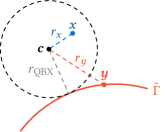
Figure 1: Illustration of the points $\boldsymbol{x}$, $\boldsymbol{y}$ and $\boldsymbol{c}$, and the ball of convergence of (3).

Inserting (3) into (2) leads to the expansion

$$\mathcal{L}[\tilde{\Gamma},\boldsymbol{\rho}](\boldsymbol{x})=\sum_{l=0}^{\infty}\sum_{m=-l}^{l}r_{x}^{l}Y_{l}^{-m}(\theta_{x},\varphi_{x})z_{lm}[\boldsymbol{\rho}]$$ (4)

of the dipole potential, where the coefficients $z_{lm}[\boldsymbol{\rho}]$ are given by

$$z_{lm}[\boldsymbol{\rho}]=\frac{4\pi}{2l+1}\int_{\tilde{\Gamma}}\boldsymbol{\rho}(\boldsymbol{y})\cdot\nabla_{\boldsymbol{y}}\frac{1}{r_{y}^{l+1}}Y_{l}^{m}(\theta_{y},\varphi_{y})\,\mathrm{d}S(\boldsymbol{y}).$$ (5)

These coefficients are complex-valued due to $Y_{l}^{m}$, but the dipole potential $\mathcal{L}$ itself is real. Since the spherical harmonics functions satisfy $Y_{l}^{-m}=(Y_{l}^{m})^{*}$, the coefficients also satisfy $z_{l,-m}=(z_{lm})^{*}$, where the asterisk denotes the complex conjugate. It is therefore enough to compute the coefficients for $m\geq 0$. The expansion (4) is in fact valid also at the point where the ball in Figure 1 touches $\tilde{\Gamma}$ (where $r_{x}=r_{\text{QBX}}$), as established in [14]. This means that the expansion can be used both for offsurface evaluation (in the interior of the ball, where the double layer potential is nearly singular) as well as onsurface evaluation (at the point on $\tilde{\Gamma}$ closest to $\boldsymbol{c}$, where the double layer potential is singular).

Relation (1) allows us to express $\boldsymbol{\mathcal{D}}$ using four dipole potentials with densities

$$\begin{array}[]{r@{\:}l}\boldsymbol{\rho}^{(j)}\>&=q_{j}\boldsymbol{n}+n_{j}\boldsymbol{q},\qquad j=1,2,3,\\[4.0pt] \boldsymbol{\rho}^{(4)}\>&=y_{k}q_{k}\boldsymbol{n}+y_{k}n_{k}\boldsymbol{q}.\end{array}$$ (6)

Each of the four dipole potentials is expanded using (4), with coefficients given by (5), which together with (1) provides a local expansion of the Stokes double layer potential.

In practice, the expansion (4) must be truncated, which is done at $l=l_{\text{max}}=p_{\text{QBX}}$. This results in the approximation

$$\mathcal{L}[\tilde{\Gamma},\boldsymbol{\rho}^{(j)}](\boldsymbol{x})\approx\mathcal{L}^{\text{QBX}}[\tilde{\Gamma},\boldsymbol{\rho}^{(j)}](\boldsymbol{x})=\sum_{l=0}^{p_{\text{QBX}}}\sum_{m=-l}^{l}r_{x}^{l}Y_{l}^{-m}(\theta_{x},\varphi_{x})z^{h}_{lm,j},\qquad j=1,2,3,4.$$ (7)

The coefficients $z^{h}_{lm,j}=z_{lm}^{h}[\boldsymbol{\rho}^{(j)}]$ are here computed using the upsampled quadrature rule introduced in section 3, with upsampling factor $\kappa=\kappa_{\text{QBX}}$. Upsampling is needed since the integrand in (5) becomes quite peaked for large $l$. However, the cost of upsampling can be entirely hidden in a precomputation step, as explained in section 3. The number of coefficients that needs to be computed in (7) for each $j$ is

$$N_{\text{QBX}}=\frac{(p_{\text{QBX}}+1)(p_{\text{QBX}}+2)}{2},$$ (8)

which takes into account that only coefficients with $m\geq 0$ need to be computed directly.

If the expansion (4) is absolutely convergent, the terms must decay in magnitude as $l\to\infty$. The size of the terms can be estimated using the bound

$$\left\lvert\sum_{m=-l}^{l}r_{x}^{l}Y_{l}^{-m}(\theta_{x},\varphi_{x})z_{lm}\right\rvert\leq r_{\text{QBX}}^{l}\sqrt{\frac{2l+1}{4\pi}}\left(\sum_{m=-l}^{l}\left\lvert z_{lm}\right\rvert^{2}\right)^{1/2},$$ (9)

where we have used the fact that [14, Eq. (3.36)]

$$\sum_{m=-l}^{l}\lvert Y_{l}^{m}(\theta,\varphi)\rvert^{2}=\frac{2l+1}{4\pi}.$$ (10)

For a single dipole expansion such as (7) with a fixed $j$, the bound (9) with $z_{lm}=z_{lm,j}^{h}$ provides a way to estimate the decay of the terms and thus the truncation error of the truncated expansion. It is however not directly applicable to the Stokes double layer potential, which involves derivatives of dipole potentials as seen in (1). To estimate the truncation error for the Stokes double layer potential, we instead evaluate the error directly in the grid points, as explained in section 2.

In summary, to compute $\boldsymbol{\mathcal{D}}[\tilde{\Gamma},\boldsymbol{q}](\boldsymbol{x})$ using QBX, the density $\boldsymbol{q}$ is first upsampled to a finer grid with upsampling factor $\kappa_{\text{QBX}}$ and then converted into four dipole densities using (6). From these, four sets of dipole coefficients $z^{h}_{lm,j}$ are computed using the direct quadrature rule on the refined grid. The coefficients are used to evaluate the dipole potentials (7), from which the Stokes double layer potential $\boldsymbol{\mathcal{D}}$ can be computed using (1). Note that the derivatives with respect to $\boldsymbol{x}$ in (1) can be computed analytically.

Since QBX can be used for both onsurface and offsurface evaluation, it is useful to introduce one expansion for each grid point. For each grid point $\boldsymbol{x}_{i}$ on the boundary, an expansion centre $\boldsymbol{c}_{i}^{+}$ is thus placed at a distance $r_{\text{QBX}}$ away from the boundary in the normal direction (i.e. in the fluid domain). This expansion centre can be used to evaluate the double layer potential in a ball touching that grid point. In practice the balls of convergence of neighbouring expansion centres will overlap, and for a given evaluation point the closest expansion centre is used to evaluate the QBX potential.

For onsurface evaluation (but not offsurface evaluation), we also use a second expansion centre $\boldsymbol{c}_{i}^{-}$ for each grid point, placed at a distance $r_{\text{QBX}}$ away from the boundary in the negative normal direction (i.e. outside the fluid domain), as shown by Figure 2. The reason for this is

Figure 2: The two expansion centres $\boldsymbol{c}_{i}^{+}$ and $\boldsymbol{c}_{i}^{-}$ used for onsurface evaluation in a grid point $\boldsymbol{x}_{i}$.

that it significantly improves the convergence when solving the boundary integral equation using GMRES, since the spectrum of the discrete operator better matches that of the continuous operator, as was noted in [29, 45, 25]. Note that due to the jump condition (2), the correct value of the potential on $\tilde{\Gamma}$ is the average of the values from the two sides:

$$\boldsymbol{\mathcal{D}}[\tilde{\Gamma},\boldsymbol{q}](\boldsymbol{x}_{i})=\frac{\boldsymbol{\mathcal{D}}^{+}[\tilde{\Gamma},\boldsymbol{q}](\boldsymbol{x}_{i})+\boldsymbol{\mathcal{D}}^{-}[\tilde{\Gamma},\boldsymbol{q}](\boldsymbol{x}_{i})}{2},$$ (11)

where $\boldsymbol{\mathcal{D}}^{+}$ is the limit from the fluid domain and $\boldsymbol{\mathcal{D}}^{-}$ is the limit from the other side of $\tilde{\Gamma}$. While using two expansions may seem to double the computational cost, the extra cost appears only in the precomputation step, as described in section 3, and thus does not affect the cost of evaluation itself.

There are two sources of error in the QBX approximation: the truncation error due to the fact that the expansion in (7) is truncated at $l=p_{\text{QBX}}$, and the coefficient error (called the “quadrature error” in [14, 25, 26]) due to the fact that the coefficients (5) are computed using a quadrature rule with finite precision. These two errors are controlled by the following three QBX parameters:

• The expansion radius $r_{\text{QBX}}$, which is the distance from the expansion centre to $\tilde{\Gamma}$ and also the radius of the ball in which the expansion is valid. Increasing $r_{\text{QBX}}$ makes the truncation error grow since the ball of convergence (and hence $r_{x}$) becomes larger, but the coefficient error decreases since the integrand in (5) becomes easier to resolve as $r_{y}$ becomes larger.

• The expansion order $p_{\text{QBX}}$, which governs the number of terms to be included in the sum in (7). Increasing $p_{\text{QBX}}$ makes the truncation error decrease since more terms are included, but the coefficient error grows since the integrand in (5) is harder to resolve for larger $l$.

• The upsampling factor $\kappa_{\text{QBX}}$, which governs the amount of grid refinement when computing the dipole coefficients (5). Increasing $\kappa_{\text{QBX}}$ makes the coefficient error decrease since the resolution of the underlying quadrature rule increases.

A simple way to decrease both the truncation error and coefficient error is to increase $p_{\text{QBX}}$ and $\kappa_{\text{QBX}}$ simultaneously while keeping $r_{\text{QBX}}$ fixed. We will continue to discuss how the QBX parameters should be selected to achieve a small overall error in section 5. For a more in-depth analysis, we refer to [14] for the truncation error, [26] for the coefficient error, as well as the summary in [25, sec. 3.5].

2 Global and local QBX

As was mentioned in section 1, a QBX method can be either (fully) global, particle-global or local, the difference being which part of the boundary (i.e. which source points) to include when forming the local expansion. Here we use particle-global QBX for particles and local QBX for walls. In essence, the difference between the three variants is what $\tilde{\Gamma}$ in section 1 is taken to be:

• For a fully global QBX method, all grid points on the whole boundary are used to form the local expansion, i.e. $\tilde{\Gamma}=\Gamma$.

• For a particle-global QBX method, all grid points on a single particle are used to form the expansion, i.e. $\tilde{\Gamma}=\Gamma_{\text{p}}^{(\alpha)}$, where $\Gamma_{\text{p}}^{(\alpha)}$ is the surface of the particle with index $\alpha$.

• For a local QBX method, only the grid points which are close to the expansion centre are used to form the expansion. In our case, we choose $\tilde{\Gamma}$ to be the $N_{\text{P}}$ patches of the wall which are closest to the expansion centre, as shown in Figure 5. (The contribution from patches further away is not included in the expansion but computed using direct quadrature.)

Note that $\tilde{\Gamma}$ may depend on the location of the expansion centre to be used, which in turn depends on the evaluation point. In principle, it is sufficient to let $\tilde{\Gamma}$ consist of the grid points close to the expansion centre (i.e. local QBX), since that is where the integrand becomes nearly singular; for grid points further away, direct quadrature can be used. The reason to extend $\tilde{\Gamma}$ further is to improve the regularity of the layer potential that is being expanded, so that the expansion converges more rapidly. Indeed, in local QBX, the expanded layer potential consists of the contribution from a truncated part of the boundary, and may not be very smooth since $\tilde{\Gamma}$ ends abruptly. However, the larger $\tilde{\Gamma}$ is, the further away from the ball of convergence will the edge of $\tilde{\Gamma}$ be, and the less will it affect the convergence of the expansion. We have observed that $N_{\text{P}}=9$ is sufficient for $\tilde{\Gamma}$ for the walls.

In particle-global QBX, the expanded layer potential has the contribution from a whole particle, which consists of a closed and smooth surface, so the potential from it should be smooth. In a fully global QBX, the expanded layer potential is the global potential, which is smooth if $\Gamma$ is regular enough. Unlike the particle-global QBX, the fully global QBX quickly becomes expensive unless a fast method (such as the FMM) is used to compute the far-field contribution. Therefore the fully global QBX variant is not used in this paper.

An advantage of the local and particle-global QBX variants over the fully global QBX is that, if the individual particles and walls are rigid, $\tilde{\Gamma}$ is the same (in local coordinates) for all particles or patches of the same shape, even if they have different orientations. This makes precomputation possible, which we shall return to in section 3. Another advantage is that expansion centres can be placed without regards to other particles or walls, since each expansion contains only the contribution from a single particle or wall segment. In a fully global QBX method, each ball of convergence must be completely outside all particles and walls, which would complicate the placement of the expansion centres.

3 Precomputation for QBX

The mapping given by (6) and the discrete version of (5), which takes the double layer density $\boldsymbol{q}$ on $\tilde{\Gamma}$ and returns the dipole coefficients $z^{h}_{lm,j}$ for a single expansion centre $\boldsymbol{c}_{i}$, is a linear function of $\boldsymbol{q}$ and can therefore be represented by a matrix $\boldsymbol{M}_{i}$. This matrix is of size $4N_{\text{QBX}}\times 3\tilde{N}$, where $N_{\text{QBX}}$ is given by (8) and $\tilde{N}$ is the number of grid points on $\tilde{\Gamma}$ (before upsampling). There is one such matrix $\boldsymbol{M}_{i}$ for every expansion centre, and it depends only on the geometry $\tilde{\Gamma}$, its discretization and the location of the expansion centre in the local coordinates of $\tilde{\Gamma}$. For a rigid geometry $\tilde{\Gamma}$, such as in our case, the matrix $\boldsymbol{M}_{i}$ can therefore be precomputed and stored.

Note that the upsampling factor $\kappa_{\text{QBX}}$ is effectively “hidden” in this precomputation step: upsampling influences the computation of $\boldsymbol{M}_{i}$ since $\boldsymbol{q}$ is upsampled before being inserted into (6), but it has no effect on the size of $\boldsymbol{M}_{i}$, which is set by the discretization of $\tilde{\Gamma}$ prior to upsampling. Therefore, upsampling does not affect the computational complexity of the method once $\boldsymbol{M}_{i}$ has been precomputed.

The matrix $\boldsymbol{M}_{i}$ which computes the coefficients $z^{h}_{lm,j}$ is used for offsurface evaluation, when the evaluation point is not known beforehand; the coefficients can then be used to evaluate the expansion at any evaluation point within the ball of convergence. For onsurface evaluation, i.e. evaluation at one of the grid points of the boundary, the evaluation point itself is known beforehand and precomputation can be taken even further. In fact, the mapping that takes the expansion coefficients to the value of the potential $\boldsymbol{\mathcal{D}}[\tilde{\Gamma},\boldsymbol{q}](\boldsymbol{x}_{i})$, given by (7) and (1), is also linear and can therefore be represented by a matrix $\boldsymbol{S}_{i}$. This allows us to compute a matrix $\boldsymbol{R}_{i}=\boldsymbol{S}_{i}\boldsymbol{M}_{i}$ which maps the density $\boldsymbol{q}$ on $\tilde{\Gamma}$ directly to the value of the double layer potential $\boldsymbol{\mathcal{D}}$ at one of the grid points – effectively representing a set of target-specific quadrature weights for every grid point. The matrix $\boldsymbol{R}_{i}$ is of size $3\times 3\tilde{N}$ and there is one such matrix for each grid point $\boldsymbol{x}_{i}$ on the boundary. Precomputing the $\boldsymbol{R}_{i}$ matrix hides not only $\kappa_{\text{QBX}}$ but also $p_{\text{QBX}}$.

Since two expansion centres are used for onsurface evaluation, as the reader may recall from Figure 2, there are actually two $\boldsymbol{R}_{i}$ matrices for each grid point: $\boldsymbol{R}_{i}^{+}$ and $\boldsymbol{R}_{i}^{-}$, associated with $\boldsymbol{c}_{i}^{+}$ and $\boldsymbol{c}_{i}^{-}$, respectively. From (11), it is clear that these matrices can be combined as

$$\boldsymbol{R}_{i}=\frac{\boldsymbol{R}_{i}^{+}+\boldsymbol{R}_{i}^{-}}{2}$$ (12)

to form a single matrix $\boldsymbol{R}_{i}$ for each grid point. This way, the extra cost of using two expansions is completely hidden in the precomputation step.

For the particles, the axisymmetry can be used to vastly reduce the amount of computations and storage needed to precompute the matrices $\boldsymbol{M}_{i}$ and $\boldsymbol{R}_{i}$. In fact, due to reflective symmetry, it suffices to compute $\boldsymbol{R}_{i}$ for the $n_{\theta}/2$ grid points ($n_{1}+n_{2}/2$ grid points for rod particles) shown in Figure 3, and $\boldsymbol{M}_{i}$ for the corresponding expansion centres. The matrices for all other grid points and their expansion centres are then calculated using rotations and reflections, as in [25]. Note that if several particles of the same shape appear in a simulation, the precomputation only needs to be done for one such particle.

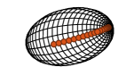
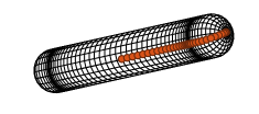
Figure 3: The matrices $\boldsymbol{M}_{i}$ and $\boldsymbol{R}_{i}$ need only be stored for the grid points along half a line of longitude, here indicated with red dots.

For a wall geometry with uniform patch size, as in our case, the geometry has a discrete translational symmetry for offsets equal to the patch size, due to periodicity. This means that the geometry “looks” exactly the same seen from any patch of the wall, and it is therefore enough to precompute the $\boldsymbol{M}_{i}$ and $\boldsymbol{R}_{i}$ matrices for the $n_{1}n_{2}$ grid points and corresponding expansion centres of a single patch of the wall. In this case $\tilde{\Gamma}$ consists of that patch and its $N_{\text{P}}-1$ closest neighbours, as indicated in Figure 5 for $N_{\text{P}}=9$.

Chapter 4 Periodicity and fast methods

Up to this point we have not taken periodicity into account in the description of the mathematical formulation and its discretization; it is now time to remedy this. We will here give the details of the periodic formulation indicated in Figure 1 (b), and in particular focus on how the special quadrature methods are combined with the fast summation method used for the periodic problem.

Consider a primary cell with side lengths $\boldsymbol{B}=(B_{1},B_{2},B_{3})$ which is replicated periodically in all three spatial directions. The flow field is then periodic, i.e. $\boldsymbol{u}(\boldsymbol{x})=\boldsymbol{u}(\boldsymbol{x}+\boldsymbol{k}\cdot\boldsymbol{B})$ for any $\boldsymbol{k}\in\mathbb{Z}^{3}$. This changes the boundary integral formulation introduced in section 1 in the following way: The layer potential $\boldsymbol{\mathcal{D}}$ and completion flow $\boldsymbol{\mathcal{V}}^{(\alpha)}$ which appear in the flow field (9) and in the fundamental boundary integral equation (10) are replaced by their periodic counterparts $\boldsymbol{\mathcal{D}}^{\text{3P}}$ and $\boldsymbol{\mathcal{V}}^{(\alpha),\text{3P}}$. These are defined as infinite sums over the periodic lattice, i.e.

$$\boldsymbol{\mathcal{D}}^{\text{3P}}[\Gamma,\boldsymbol{q}](\boldsymbol{x})=\sum_{\boldsymbol{k}\in\mathbb{Z}^{3}}\boldsymbol{\mathcal{D}}[\Gamma,\boldsymbol{q}](\boldsymbol{x}+\boldsymbol{k}\cdot\boldsymbol{B}),\qquad\boldsymbol{\mathcal{V}}^{(\alpha),\text{3P}}[\boldsymbol{F},\boldsymbol{\tau}](\boldsymbol{x})=\sum_{\boldsymbol{k}\in\mathbb{Z}^{3}}\boldsymbol{\mathcal{V}}^{(\alpha)}[\boldsymbol{F},\boldsymbol{\tau}](\boldsymbol{x}+\boldsymbol{k}\cdot\boldsymbol{B}).$$ (1)

These sums converge slowly, and their value depends on the order of summation, so they cannot be computed using direct summation. We compute them using the Spectral Ewald (SE) method [31, 32], a fast Ewald summation method based on the fast Fourier transform (FFT). The SE method is described in detail for the stokeslet in [31], for the stresslet in [23] and for the rotlet in [24], and has been combined with QBX previously in [25]. In the SE method, each of the periodic sums in (1) is split into two parts: the real-space part, which decays fast and can therefore be summed directly in real space; and the Fourier-space part, which is smooth and therefore decays fast in Fourier space.

No special treatment is needed for the completion flow $\boldsymbol{\mathcal{V}}^{(\alpha),\text{3P}}$ since the evaluation point is never close to the singular points (which are inside the particle), so the SE method as described in [31, 24] is used without modification. For the double layer potential $\boldsymbol{\mathcal{D}}^{\text{3P}}$, special quadrature is needed so SE must be combined with QBX and the upsampled quadrature rule. How this is done is described below.

The periodic sum for the double layer potential can be written explicitly as

$$\mathcal{D}_{i}^{\text{3P}}[\Gamma,\boldsymbol{q}](\boldsymbol{x})=\sum_{\boldsymbol{k}\in\mathbb{Z}^{3}}\int_{\Gamma}T_{ijl}(\boldsymbol{x}+\boldsymbol{k}\cdot\boldsymbol{B}-\boldsymbol{y})q_{j}(\boldsymbol{y})n_{l}(\boldsymbol{y})\,\mathrm{d}S(\boldsymbol{y}).$$ (2)

The stresslet $\boldsymbol{T}$ is split into two parts

$$T_{ijl}(\boldsymbol{r})=T_{ijl}^{\text{R}}(\boldsymbol{r};\xi)+T_{ijl}^{\text{F}}(\boldsymbol{r};\xi),$$ (3)

where $\boldsymbol{T}^{\text{R}}$ is the real-space part and $\boldsymbol{T}^{\text{F}}$ is the Fourier-space part. The Ewald parameter $\xi$ is a positive number which is used to balance the decay of $\boldsymbol{T}^{\text{R}}$ in real space and the decay of the Fourier coefficients of $\boldsymbol{T}^{\text{F}}$ (a larger value of $\xi$ makes the real-space part decay faster and the Fourier-space part decay slower, thus shifting computational work into Fourier space). In the split that we use, $\boldsymbol{T}^{\text{R}}$ is given by [23, 25]

$$T_{ijl}^{\text{R}}(\boldsymbol{r};\xi) =-\frac{2}{r^{4}}\left(\frac{3}{r}\operatorname{erfc}(\xi r)+\frac{2\xi}{\sqrt{\pi}}(3+2\xi^{2}r^{2}-4\xi^{4}r^{4})\mathrm{e}^{-\xi^{2}r^{2}}\right)r_{i}r_{j}r_{l}$$

$$\phantom{=\>\,}+\frac{8\xi^{3}}{\sqrt{\pi}}(2-\xi^{2}r^{2})\mathrm{e}^{-\xi^{2}r^{2}}(\delta_{ij}r_{l}+\delta_{jl}r_{i}+\delta_{li}r_{j}),$$ (4)

where $r=\lvert\boldsymbol{r}\rvert$. The Fourier-space part is simply given by $\boldsymbol{T}^{\text{F}}=\boldsymbol{T}-\boldsymbol{T}^{\text{R}}$. Inserting (3) into (2) splits the periodic double layer potential into two parts $\boldsymbol{\mathcal{D}}^{\text{3P}}=\boldsymbol{\mathcal{D}}^{\text{3P,R}}+\boldsymbol{\mathcal{D}}^{\text{3P,F}}$, where

$$\mathcal{D}_{i}^{\text{3P,R}}[\Gamma,\boldsymbol{q}](\boldsymbol{x};\xi) =\sum_{\boldsymbol{k}\in\mathbb{Z}^{3}}\int_{\Gamma}T_{ijl}^{\text{R}}(\boldsymbol{x}+\boldsymbol{k}\cdot\boldsymbol{B}-\boldsymbol{y};\xi)q_{j}(\boldsymbol{y})n_{l}(\boldsymbol{y})\,\mathrm{d}S(\boldsymbol{y}),$$ (5)

$$\mathcal{D}_{i}^{\text{3P,F}}[\Gamma,\boldsymbol{q}](\boldsymbol{x};\xi) =\sum_{\boldsymbol{k}\in\mathbb{Z}^{3}}\int_{\Gamma}T_{ijl}^{\text{F}}(\boldsymbol{x}+\boldsymbol{k}\cdot\boldsymbol{B}-\boldsymbol{y};\xi)q_{j}(\boldsymbol{y})n_{l}(\boldsymbol{y})\,\mathrm{d}S(\boldsymbol{y}).$$ (6)

The singularity of the stresslet is completely transferred to $\boldsymbol{T}^{\text{R}}$, while $\boldsymbol{T}^{\text{F}}$ is nonsingular [25]. The Fourier-space part (6) is computed using FFTs as described in appendix D and [23]. The real-space potential (5) is evaluated in real space, and requires special quadrature due to the singularity of $\boldsymbol{T}^{\text{R}}$, much as in the free-space setting. Note that since $\boldsymbol{T}^{\text{R}}(\boldsymbol{r};\xi)$ decays fast as $\lvert\boldsymbol{r}\rvert\to\infty$ it can be neglected for $\lvert\boldsymbol{r}\rvert>r_{\text{c}}$, where $r_{\text{c}}$ is called the cutoff radius. We can thus change the integration domain in (5) to $\Gamma^{\star}=\Gamma^{\star}(\boldsymbol{x},\boldsymbol{k};r_{\text{c}})=\{\boldsymbol{y}\in\Gamma:\lvert\boldsymbol{x}+\boldsymbol{k}\cdot\boldsymbol{B}-\boldsymbol{y}\rvert\leq r_{\text{c}}\}$ and approximate

$$\mathcal{D}_{i}^{\text{3P,R}}[\Gamma,\boldsymbol{q}](\boldsymbol{x};\xi)\approx\mathcal{D}_{i}^{\text{3P,R}\star}[\Gamma,\boldsymbol{q}](\boldsymbol{x};\xi)=\sum_{\boldsymbol{k}\in\mathbb{Z}^{3}}\int_{\Gamma^{\star}}T_{ijl}^{\text{R}}(\boldsymbol{x}+\boldsymbol{k}\cdot\boldsymbol{B}-\boldsymbol{y};\xi)q_{j}(\boldsymbol{y})n_{l}(\boldsymbol{y})\,\mathrm{d}S(\boldsymbol{y}).$$ (7)

The error of this approximation is determined by the product $\xi r_{\text{c}}$ as described in [23]. Rather than deriving a new QBX expansion from scratch for the real-space part $\boldsymbol{\mathcal{D}}^{\text{3P,R}\star}$, we reuse the expansion of the total layer potential $\boldsymbol{\mathcal{D}}$ from section 3. To be able to do this, we insert $\boldsymbol{T}^{\text{R}}=\boldsymbol{T}-\boldsymbol{T}^{\text{F}}$ into (7) to get

$$\mathcal{D}_{i}^{\text{3P,R}\star}[\Gamma,\boldsymbol{q}](\boldsymbol{x};\xi) =\sum_{\boldsymbol{k}\in\mathbb{Z}^{3}}\int_{\Gamma^{\star}}T_{ijl}(\boldsymbol{x}+\boldsymbol{k}\cdot\boldsymbol{B}-\boldsymbol{y};\xi)q_{j}(\boldsymbol{y})n_{l}(\boldsymbol{y})\,\mathrm{d}S(\boldsymbol{y})$$ (8)

$$\phantom{=}-\sum_{\boldsymbol{k}\in\mathbb{Z}^{3}}\int_{\Gamma^{\star}}T_{ijl}^{\text{F}}(\boldsymbol{x}+\boldsymbol{k}\cdot\boldsymbol{B}-\boldsymbol{y};\xi)q_{j}(\boldsymbol{y})n_{l}(\boldsymbol{y})\,\mathrm{d}S(\boldsymbol{y}).$$ (9)

Note that the integration domain $\Gamma^{\star}$ ensures that both of these sums have few terms since $r_{\text{c}}$ should be small – typically smaller than the size of the periodic cell. The integral in (8) represents the total layer potential from $\Gamma^{\star}$ and can thus be computed using the combined special quadrature method from section 3, with truncation at $r_{\text{c}}$. The integral in (9) is computed using direct quadrature, which is possible since $\boldsymbol{T}^{\text{F}}$ is nonsingular.

As in the free-space setting in section 3, the evaluation point $\boldsymbol{x}$ is classified into one of three regions (see Figure 7). The potential is evaluated using (7) in the direct quadrature region and (8)–(9) in the other two regions. The reader may wonder why we in the upsampled quadrature region do not simply evaluate (7) using upsampled quadrature. The reason is that (9) evaluated using the same quadrature method as in the Fourier-space part—i.e. direct quadrature—is needed to cancel discretization errors in the latter. These discretization errors may be larger than the SE error tolerance and are caused by the fact that $\boldsymbol{T}^{\text{F}}(\boldsymbol{r};\xi)$, while nonsingular, tends to become slightly peaked for small $\lvert\boldsymbol{r}\rvert$, i.e. close to $\Gamma^{\star}$. Cancellation prevents these errors from influencing the error of the full method.

Another important point to note is that $r_{\text{c}}$ must be chosen large enough so that no special quadrature is needed for the total potential when $\lvert\boldsymbol{r}\rvert>r_{\text{c}}$. This is because, for $\lvert\boldsymbol{r}\rvert>r_{\text{c}}$, the total potential is equal to the Fourier-space part, which is always computed using direct quadrature. Thus, $r_{\text{c}}$ must be at least as large as the distance from $\Gamma$ to the direct quadrature region.

Chapter 5 Parameter selection

In this section, we develop our strategy for selecting the parameters of the combined special quadrature, i.e. upsampled quadrature and QBX, when evaluating the Stokes double layer potential $\boldsymbol{\mathcal{D}}$. We assume that a discretization of the geometry is given, with sufficient resolution for the density to be well-resolved and the direct quadrature to achieve a given error tolerance $\varepsilon_{\text{tol}}$ at a given distance (sufficiently far away) from all surfaces. The goal is to select quadrature parameters for each particle and wall so that the error tolerance $\varepsilon_{\text{tol}}$ is achieved also in the upsampled quadrature region and QBX region. Of course, there are many different ways to choose the parameters, some resulting in higher computational efficiency than others. Here, we do not aim to optimize the efficiency; instead, our focus is on achieving the given error tolerance at an acceptable (albeit not optimal) computational cost.

The parameters that must be selected are shown in Figure 1. Note that we allow for multiple upsampled quadrature regions with different upsampling factors $\kappa_{\text{U$i$}}$, in order to gradually increase the upsampling closer to the surface. Due to the precomputation scheme for QBX, using QBX may in fact be faster than using upsampled quadrature with the same upsampling factor. Therefore, the QBX region may extend further away from the surface than the expansion centre (i.e. $d_{\text{QBX}}$ may be larger than $r_{\text{QBX}}$, but of course not larger than $2r_{\text{QBX}}$).

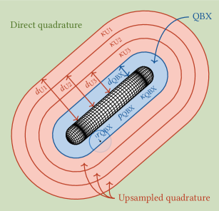
Figure 1: Parameters of the combined special quadrature, here for a rod with $N_{\text{U}}=3$ upsampled quadrature regions (each geometrical object has its own set of corresponding parameters). Note that while the ball of convergence for QBX can be larger than the QBX region, the expansion is used only inside the QBX region.

The parameters to be selected are as follows:

• The threshold distances $d_{\text{U$i$}}$ for the upsampled quadrature regions, $i=1,2,\ldots,N_{\text{U}}$, and the threshold distance $d_{\text{QBX}}$ for the QBX region. These determine at what distance from the surface each region starts. If $d_{\Gamma}(\boldsymbol{x})$ is the distance from the evaluation point $\boldsymbol{x}$ to the surface $\Gamma$, then $\boldsymbol{x}$ belongs to the $i$th upsampled quadrature region if

  $$d_{\text{U$i$}}\geq d_{\Gamma}(\boldsymbol{x})\geq\begin{cases}d_{\text{U$(i+1)$}}&\text{if $i<N_{\text{U}}$}\\ d_{\text{QBX}}&\text{if $i=N_{\text{U}}$},\end{cases}$$ (1)

  and $\boldsymbol{x}$ belongs to the QBX region if $d_{\text{QBX}}\geq d_{\Gamma}(\boldsymbol{x})\geq 0$. Each of these distances should be chosen so that the error does not exceed the tolerance in the region further away from the surface (for example, $d_{\text{U1}}$ is selected based on the direct quadrature error).

• The upsampling factors $\kappa_{\text{U$i$}}$ for the upsampled quadrature regions, $i=1,2,\ldots,N_{\text{U}}$. These should be increasing, i.e. $\kappa_{\text{U1}}<\kappa_{\text{U2}}<\ldots<\kappa_{\text{U$N_{\text{U}}$}}$. The upsampling factor $\kappa_{\text{U$i$}}$ determines the distance $d_{\text{U$(i+1)$}}$ at which the next region must begin, which we will come back to in section 1.

• The QBX upsampling factor $\kappa_{\text{QBX}}$, which controls the amount of upsampling used when computing the coefficients in (5), and thus the QBX coefficient error as mentioned in section 1. It should be chosen large enough so that the coefficient error and the truncation error are balanced. The upsampling factor influences the QBX precomputation time (which grows like $O(\kappa_{\text{QBX}}^{2})$), but not the size of the precomputed $\boldsymbol{M}_{i}$ and $\boldsymbol{R}_{i}$ matrices, and thus not the evaluation time.

• The QBX expansion order $p_{\text{QBX}}$, which controls the number of terms included in the expansion in (7), and thus the QBX truncation error as mentioned in section 1. It should be chosen so that the truncation error is below the error tolerance everywhere in the QBX region. The expansion order affects the size of the $\boldsymbol{M}_{i}$ matrix used for offsurface evaluation (which grows like $O(p_{\text{QBX}}^{2})$), but not that of the $\boldsymbol{R}_{i}$ matrix used for onsurface evaluation. It should be noted that as $p_{\text{QBX}}$ increases, the upsampling factor $\kappa_{\text{QBX}}$ must also increase since higher-order coefficients are harder to resolve.

• The QBX expansion radius $r_{\text{QBX}}$, which affects both the coefficient error and the truncation error, but neither the precomputation time nor the evaluation time directly. It should typically be chosen as small as possible, since this speeds up the convergence of the expansion in (7) so that $p_{\text{QBX}}$ can be chosen small. On the other hand, a very small $r_{\text{QBX}}$ means that the upsampling factor $\kappa_{\text{QBX}}$ must be large, since the expansion centre moves closer to the surface.

  However, in our implementation the primary restriction on $r_{\text{QBX}}$ is that it must be large enough for the balls of convergence to cover the QBX region sufficiently well. In general, $r_{\text{QBX}}$ should not be smaller than the distance from one expansion centre to the next, to ensure a good coverage. Since we have one expansion centre per grid point, we require that $r_{\text{QBX}}$ should not be smaller than the grid spacing. Letting $h$ be some measure of the grid spacing (for example the largest distance between neighbouring grid points on the surface), it is useful to consider the ratio $r_{\text{QBX}}/h$ when selecting parameters. As noted in [25], this has the advantage that if $r_{\text{QBX}}/h$ is kept fixed during refinement of the original grid, then the coefficient error is constant, assuming that the upsampling factor $\kappa_{\text{QBX}}$ is also fixed. We will therefore consider $r_{\text{QBX}}/h$ in the rest of this section.

Unfortunately, no general error estimates are available in three dimensions for the quadrature rules that we use here. The parameters must therefore be selected based on numerical experiments, and we present a strategy for doing so here. The idea is to start from the outermost upsampled quadrature region (U1) and then proceed inwards towards the surface of the particle or wall, determining the parameters in the following order:

1. Threshold distances and upsampling factors for the upsampled quadrature regions,

2. The QBX parameters $r_{\text{QBX}}/h$ and $d_{\text{QBX}}$,

3. The QBX parameters $p_{\text{QBX}}$ and $\kappa_{\text{QBX}}$.

The process must be repeated for each type of particle and wall to be used. We develop the strategy in the context of a specific rod particle in section 1; a summary of the parameter selection strategy in the general case follows in section 2. In sections 3 and 4 we apply the strategy to two more examples (a rod with a higher aspect ratio and a plane wall).

In order to estimate the error during the parameter selection process, we apply a constant density $\tilde{\boldsymbol{q}}$ such that $\lvert\tilde{\boldsymbol{q}}\rvert=1$ to the surface and evaluate the stresslet identity (3). This may seem like an overly simple test case since both the density and the solution are constant. However, the QBX expansions are not of the constant double layer potential $\boldsymbol{\mathcal{D}}$ itself, but of the four dipole potentials $\mathcal{L}$ defined by (1), and these are not constant. In practice, the stresslet identity seems to provide a decent test case for both direct quadrature, upsampled quadrature and QBX, as shown by the results in section 2 where the density is not constant.

The Spectral Ewald parameters $\xi$ and $r_{\text{c}}$ will not be discussed at length here, but we note that the requirement that no special quadrature be needed for $\lvert\boldsymbol{r}\rvert>r_{\text{c}}$ implies that $r_{\text{c}}$ must be at least as large as $d_{\text{U1}}$. The Spectral Ewald error is determined by the product $\xi r_{\text{c}}$ in real space and $\xi h_{\text{F}}$ in Fourier space, where $h_{\text{F}}$ is the grid spacing of the uniform grid used for the Fourier-space part (see appendix D). Given a tolerance $\varepsilon_{\text{tol}}$, the parameters $\xi$, $r_{\text{c}}$ and $h_{\text{F}}$ must satisfy the system $\xi r_{\text{c}}=A(\varepsilon_{\text{tol}})$, $\xi h_{\text{F}}=B(\varepsilon_{\text{tol}})$, where $A$ and $B$ are known functions. This leaves one degree of freedom which can be used to minimize the computational cost, albeit under the constraint $r_{\text{c}}\geq d_{\text{U1}}$. For a general discussion on the selection of Spectral Ewald parameters, including the functions $A$ and $B$, we refer to [23] for the stresslet, [31] for the stokeslet, and [24] for the rotlet.

1 Introductory example: a rod particle with low aspect ratio

In this first example, we consider a rod particle of length $L=2$ and radius $R=0.5$ (i.e. aspect ratio 2), shown in Figure 2. The grid used for the direct quadrature has parameters $n_{1}=40$, $n_{2}=10$ and $n_{\varphi}=25$ (introduced in section 1), for a total of 2250 grid points. To give an idea of the error associated with the direct quadrature, we apply the constant density $\tilde{\boldsymbol{q}}=(1,1,1)/\sqrt{3}$ to the particle surface and compute the stresslet identity (3) using direct quadrature in two planes intersecting the particle. The absolute error in these planes is shown in Figure 2.

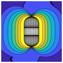
(a) Direct quadrature error, slice 1

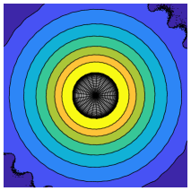
(b) Direct quadrature error, slice 2

(c)

Figure 2: Error in two perpendicular slices (a) and (b) through the rod particle, when evaluating the stresslet identity (3) using direct quadrature in free space.

To determine how the error varies with the distance to the surface, we evaluate (3) along several normal lines centred on grid points of the particle; due to the symmetry of the error it is enough to consider the $n_{1}+n_{2}/2=45$ lines shown in Figure 3 (a). The error along these lines is shown in Figure 3 (b). Given an error tolerance $\varepsilon_{\text{tol}}$, the smallest distance at which the error does not exceed $\varepsilon_{\text{tol}}$ can be determined numerically. This distance is taken as $d_{\text{U1}}$. In this example, we will use the error tolerance $\varepsilon_{\text{tol}}=${10}^{-10}$$. As indicated in Figure 3 (b), the error reaches ${10}^{-10}$ at $d_{\text{U1}}=1.061$; special quadrature must be used within this distance to the surface. Having established the first threshold distance $d_{\text{U1}}$, we now proceed to determine the rest of the parameters for the upsampled quadrature regions, in section 1.

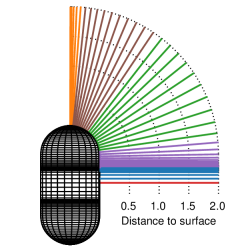
(a) Lines along which the error is plotted

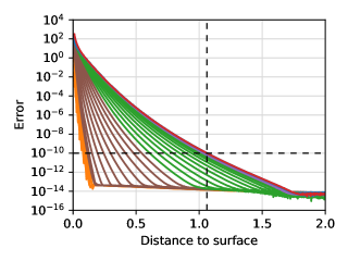
(b) Direct quadrature error along the lines

Figure 3: Error of the direct quadrature along 45 normal lines centred on grid points of the particle surface. In (a), the normal lines are shown coloured in groups of ten. In (b), the error along each line is shown with the same colours (here, the blue and purple curves are obscured by the red curve). The line with the greatest error is coloured red; the error along this line reaches the value ${10}^{-10}$ at distance 1.061 from the surface. (The smallest distance to surface included here is 0.01.)

1 Parameters for the upsampled quadrature regions

For the sake of simplicity we will always choose the upsampling factors to be $\kappa_{\text{U$i$}}=i+1$, meaning that the first upsampling factor will be $\kappa_{\text{U1}}=2$, the next will be $\kappa_{\text{U2}}=3$ and so on (this may not be the optimal strategy with regard to computational cost, but recall that our goal is not to optimize for computational efficiency). In order to determine the threshold distance $d_{\text{U$i$}}$ of every upsampled quadrature region, we repeat the investigation from Figure 3 for different upsampling factors $\kappa=1,2,3,\ldots$, computing the stresslet identity error as a function of the distance to the surface for each upsampling factor. The maximal error at each distance is shown in Figure 4 ($\kappa=1$ corresponds to Figure 3). The threshold distance $d_{\text{U$(i+1)$}}$ is now taken as the distance at which the error curve corresponding to $\kappa=\kappa_{\text{U$i$}}$ intersects the error tolerance $\varepsilon_{\text{tol}}$ ($i=1,2,\ldots$). For instance, in this case the curve corresponding to $\kappa=\kappa_{\text{U1}}=2$ intersects $\varepsilon_{\text{tol}}=${10}^{-10}$$ around $0.391=d_{\text{U2}}$.

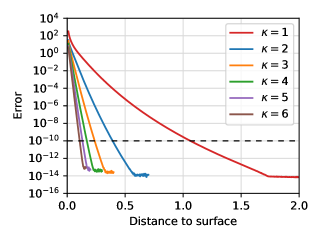
Figure 4: Maximal stresslet identity error along any of the lines shown in Figure 3 (a), for upsampled quadrature with different upsampling factors $\kappa$. (The smallest distance to surface included here is 0.01.)

This procedure sets all of the parameters for the upsampled quadrature, as shown in Table 1. However, at some point we must switch from upsampled quadrature to QBX, which is determined by the QBX threshold distance $d_{\text{QBX}}$. Selecting $d_{\text{QBX}}$ will also fix the number of upsampled quadrature regions $N_{\text{U}}$. We will determine $d_{\text{QBX}}$ together with the other QBX parameters in section 2.

Table 1: Parameters for the upsampled quadrature regions, tolerance ${10}^{-10}$.

$i$	1	2	3	4	5	6	$\cdots$
$\kappa_{\text{U$i$}}$	2	3	4	5	6	7	$\cdots$
$d_{\text{U$i$}}$	1.061	0.391	0.237	0.169	0.132	0.108	$\cdots$

2 Parameters for the QBX region

To understand how the QBX error behaves, we plot the offsurface error from a single expansion in Figure 5 (a). Note that the QBX parameters used in this figure are not yet selected to achieve the error tolerance, but meant only to demonstrate the general behaviour of the error. Since the QBX error is the largest at the boundary of the ball of convergence (outside this ball the direct quadrature error is shown in Figure 5 (a)), it is sufficient to measure the error at a point on this boundary, for example at the point where the ball touches the particle. Thus, we measure the QBX error at all the grid points of the rod – the onsurface error – shown in Figure 5 (b) for these particular QBX parameters.

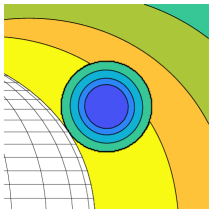
(a) Offsurface error from a single QBX expansion

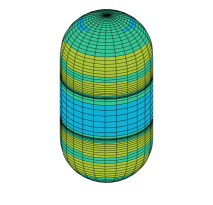
(b) Onsurface error

QBX expansion

(c)

QBX expansion

Figure 5: Error when evaluating the stresslet identity (3) using quadrature by expansion with the parameters $r_{\text{QBX}}=h=\pi/25$, $p_{\text{QBX}}=18$ and $\kappa_{\text{QBX}}=15$: (a) in a slice through the particle centre (i.e. offsurface), using a single QBX expansion centre and direct quadrature outside the ball of convergence; (b) in the grid points of the particle (i.e. onsurface). Note in (b) that the error seems to be related to the curvature of the boundary; in particular the error is larger in areas where the curvature changes, viz. in the smooth transition from cylinder to cap. (Similar observations related to the convexity of the boundary were reported in [3] and [29].)

For particles, we define the grid spacing $h$ as the distance between grid points in the azimuthal direction at the equator of the particle, i.e.

$$h=\frac{2\pi R}{n_{\varphi}}\leavevmode\nobreak\ \text{for rods},\hskip 80.00012pth=\frac{2\pi a}{n_{\varphi}}\leavevmode\nobreak\ \text{for spheroids},$$ (2)

where $n_{\varphi}$ is the number of grid points in the azimuthal direction (as defined in section 1), $R$ is the radius of the rod and $a$ is the equatorial semiaxis of the spheroid (which appears in (6)). For the rod that we consider in this example, $R=0.5$ and $n_{\varphi}=25$, so $h=\pi/25\approx 0.1257$.

We now focus on selecting the parameters $r_{\text{QBX}}/h$, $p_{\text{QBX}}$ and $\kappa_{\text{QBX}}$ such that the error is bounded by $\varepsilon_{\text{tol}}$ in the whole ball of convergence, for all QBX expansions of the particle. To do this, we consider the maximal onsurface error as we vary these three parameters, shown in Figure 6. As seen in Figure 6 (a), $r_{\text{QBX}}/h$ should be chosen as small as possible since this improves the decay of the truncation error as $p_{\text{QBX}}$ grows; if $r_{\text{QBX}}/h$ is small, $p_{\text{QBX}}$ can also be chosen small, which is important since the offsurface evaluation time for QBX grows as $O(p_{\text{QBX}}^{2})$. On the other hand, as Figure 7 shows, $r_{\text{QBX}}$ must not be too small compared to $h$, since then the balls of convergence would not overlap properly, and large areas of the QBX region would not be covered by any ball of convergence. For this reason we require that $r_{\text{QBX}}\geq h$. In fact, since $r_{\text{QBX}}$ should be as small as possible, we will always set $r_{\text{QBX}}=h$, so that $r_{\text{QBX}}/h=1$.

To select $p_{\text{QBX}}$ and $\kappa_{\text{QBX}}$, we use the data shown in Figure 6 (b), which is for $r_{\text{QBX}}/h=1$. As can be seen there, the truncation error is independent of $\kappa_{\text{QBX}}$ and depends only on $p_{\text{QBX}}$, so we simply select the smallest $p_{\text{QBX}}$ such that the truncation error is below the tolerance. Then we select the smallest $\kappa_{\text{QBX}}$ (restricted to multiples of five for convenience) such that the coefficient error is no larger than the truncation error (i.e. such that the minimum point of the error curve is to the right of the selected $p_{\text{QBX}}$). For example, for $\varepsilon_{\text{tol}}=${10}^{-10}$$, we must choose $p_{\text{QBX}}=40$ and $\kappa_{\text{QBX}}=20$.

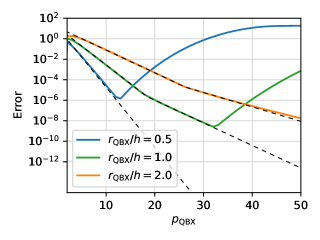
(a) Onsurface QBX error for different $r_{\text{QBX}}/h$

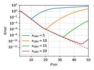
(b) Onsurface QBX error for different $\kappa_{\text{QBX}}$

Figure 6: Maximal onsurface error on the rod when evaluating the stresslet identity using QBX. In (a) for different $r_{\text{QBX}}/h$ with $\kappa_{\text{QBX}}=15$ fixed, and in (b) for different $\kappa_{\text{QBX}}$ with $r_{\text{QBX}}/h=1$ fixed. Note that each curve has a minimum, which is where the truncation error (which decreases as $p_{\text{QBX}}$ grows) and the coefficient error (which increases as $p_{\text{QBX}}$ grows) balance. The dashed lines indicate the experimental truncation error estimate (3).

It remains to choose the threshold distance $d_{\text{QBX}}$, which determines the extent of the QBX region as shown in Figure 7. Clearly $d_{\text{QBX}}$ cannot be larger than $2r_{\text{QBX}}$ since then the balls of convergence would not reach the edge of the QBX region. Even with $d_{\text{QBX}}=2r_{\text{QBX}}$, there would be areas in the QBX region, close to its edge, that would not be inside any ball of convergence. To mitigate this problem, we introduce a safety factor $\gamma$, derived in appendix C, and require that

$$d_{\text{QBX}}\leq 2\gamma r_{\text{QBX}},$$ (4)

where $\gamma=0.85$. As long as $d_{\text{QBX}}$ satisfies (4), it can be chosen arbitrarily, in the sense that its value will not affect

Figure 7: Balls of convergence with the parameters $r_{\text{QBX}}$ and $d_{\text{QBX}}$ and the grid spacing $h$ marked.

the conformance to the error tolerance, only the computational cost. We introduce the somewhat arbitrary additional constraint that $d_{\text{QBX}}\geq r_{\text{QBX}}$, and then select $d_{\text{QBX}}$ as follows: If the interval $[r_{\text{QBX}},2\gamma r_{\text{QBX}}]$ contains any threshold distance $d_{\text{U$i$}}$ for the upsampled quadrature regions, set $d_{\text{QBX}}$ equal to the largest $d_{\text{U$i$}}$ in the interval (i.e. the one with the smallest $i$). Otherwise, set $d_{\text{QBX}}=r_{\text{QBX}}$. In any case, this also sets the number of upsampled quadrature regions $N_{\text{U}}$ since the last upsampled quadrature region ends where the QBX region begins. Our choices here are motivated by keeping $N_{\text{U}}$ as low as possible since this reduces the computational cost, which we will return to in section 4.

In our current example, $d_{\text{QBX}}$ should be in the interval $[r_{\text{QBX}},2\gamma r_{\text{QBX}}]\approx[0.1257,0.2136]$. As seen in Table 1, $d_{\text{U4}}=0.169$ is the largest threshold distance in this interval, and thus we select $d_{\text{QBX}}=0.169$ which means that $N_{\text{U}}=3$ upsampled quadrature regions are used.

3 Verification of selected parameters

To summarize, the parameters that were selected above for the rod in this example was, with error tolerance ${10}^{-10}$,

$$\begin{array}[]{r@{\:}c@{\:}l@{\qquad}r@{\:}c@{\:}l@{\qquad}r@{\:}c@{\:}l}r_{\text{QBX}}/h\>&=\hfil\>&1,&N_{\text{U}}\>&=\hfil\>&3,\\ d_{\text{QBX}}\>&=\hfil\>&0.169,&d_{\text{U1}}\>&=\hfil\>&1.061,&\kappa_{\text{U1}}\>&=\hfil\>&2,\\ p_{\text{QBX}}\>&=\hfil\>&40,&d_{\text{U2}}\>&=\hfil\>&0.391,&\kappa_{\text{U2}}\>&=\hfil\>&3,\\ \kappa_{\text{QBX}}\>&=\hfil\>&20,&d_{\text{U3}}\>&=\hfil\>&0.237,&\kappa_{\text{U3}}\>&=\hfil\>&4.\\ \end{array}$$ (5)

If the selected QBX upsampling factor $\kappa_{\text{QBX}}$ seems large, recall that this parameter is completely hidden in the QBX precomputation step, as explained in section 3. To verify that the selected parameters keep the error below the tolerance, we plot in Figure 8 (a) the maximum error along the 45 lines that were used earlier (shown in Figure 3 (a)). We also plot the error in two slices in Figure 9. The fact that the error slightly exceeds the tolerance at some points in (b) should come as no surprise, since we have used the error only along certain lines to select the parameters, not in the whole space. All the points where the tolerance is exceeded are close to the boundary between different quadrature regions and could thus be eliminated by adjusting the threshold distances slightly upwards (which we will however not do here).

The parameter selection procedure is repeated for the same rod with the looser error tolerance ${10}^{-6}$. The parameters for tolerance ${10}^{-6}$ are

$$\begin{array}[]{r@{\:}c@{\:}l@{\qquad}r@{\:}c@{\:}l@{\qquad}r@{\:}c@{\:}l}r_{\text{QBX}}/h\>&=\hfil\>&1,&N_{\text{U}}\>&=\hfil\>&2,\\ d_{\text{QBX}}\>&=\hfil\>&0.149,&d_{\text{U1}}\>&=\hfil\>&0.575,&\kappa_{\text{U1}}\>&=\hfil\>&2,\\ p_{\text{QBX}}\>&=\hfil\>&21,&d_{\text{U2}}\>&=\hfil\>&0.238,&\kappa_{\text{U2}}\>&=\hfil\>&3,\\ \kappa_{\text{QBX}}\>&=\hfil\>&15,\\ \end{array}$$ (6)

and the error is shown in Figure 8 (b) and Figure 10.

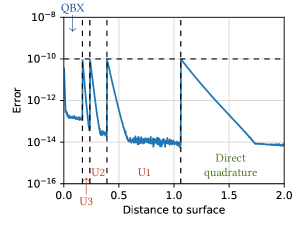
(a) Special quadrature error, tolerance ${10}^{-10}$

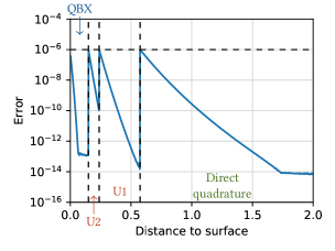
(b) Special quadrature error, tolerance ${10}^{-6}$

Figure 8: Maximal stresslet identity error along any of the lines shown in Figure 3 (a) as a function of the distance to the surface (for 1000 equispaced distances in $[0,2]$), using the combined special quadrature with (a) tolerance ${10}^{-10}$ and (b) tolerance ${10}^{-6}$. The different quadrature regions are marked. The largest error is $9.709\text{\times}{10}^{-11}$ in (a), and $9.995\text{\times}{10}^{-7}$ in (b).

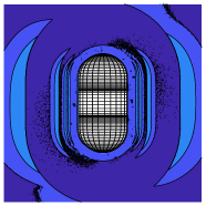
(a) Special quadrature error,

tolerance ${10}^{-10}$, slice 1

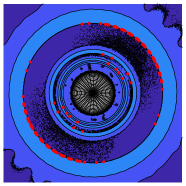
(b) Special quadrature error,

tolerance ${10}^{-10}$, slice 2

(c)

tolerance

Figure 9: Error in two perpendicular slices (a) and (b) through the rod particle, when evaluating the stresslet identity (3) using combined special quadrature with tolerance ${10}^{-10}$ in free space. Each slice consists of $500\times 500$ evaluation points. All points in (a) are below the tolerance, but 166 points in (b), marked red, are above the tolerance. The largest error is $9.768\text{\times}{10}^{-11}$ in (a) and $1.074\text{\times}{10}^{-10}$ in (b).

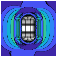
(a) Special quadrature error,

tolerance ${10}^{-6}$, slice 1

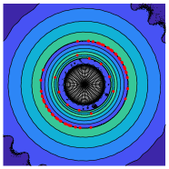
(b) Special quadrature error,

tolerance ${10}^{-6}$, slice 2

(c)

Figure 10: Error in two perpendicular slices (a) and (b) through the rod particle, when evaluating the stresslet identity (3) using combined special quadrature with tolerance ${10}^{-6}$ in free space. Each slice consists of $500\times 500$ evaluation points. All points in (a) are below the tolerance, but 90 points in (b), marked red, are above the tolerance. The largest error is $9.214\text{\times}{10}^{-7}$ in (a) and $1.079\text{\times}{10}^{-6}$ in (b).

4 A note on the computational cost

While our parameter selection strategy does not try to optimize the computational cost, we naturally strive for a reasonably low cost. We therefore comment on the computational cost for the different quadrature methods considered here. The computational complexity for evaluating the layer potential using each quadrature method is shown in Table 2. The precomputation time (for constructing the interpolation matrices and QBX matrices), which is naturally independent of the number of evaluation points, is not included. Note that the total evaluation time depends on the number of evaluation points in each quadrature region, and also on the number of expansions that are used for the evaluation points in the QBX region (recall that the closest expansion centre is used for each evaluation point).

An example of evaluation times for a specific computer machine is given in Table 3, again excluding precomputation. The time required to find the closest expansion centre for each evaluation point in the QBX region has been omitted from Tables 2 and 3 since it is negligible (around $${10}^{-8}$\times N_{\text{eval,QBX}}$ seconds).

For a particle, $N_{\text{grid}}$ is the number of grid points on the whole particle, i.e. $N_{\text{grid}}=2250$ for the rod that we have considered so far. Let us study the special case of a single evaluation point, relevant for example when computing a streamline. Based on Table 3, the evaluation time for this single point can be computed, depending on which quadrature region the point belongs to and the parameter $\kappa_{\text{U$i$}}$ or $p_{\text{QBX}}$. This is shown in Table 4. From this, it can for example be seen that the evaluation takes roughly 1000 times longer for a point in the upsampled quadrature region with $\kappa_{\text{U$i$}}=2$ compared to the direct quadrature region. (The upsampled quadrature cost is in this case completely dominated by interpolating the density, i.e. multiplying it by the precomputed interpolation matrix.)

Table 2: Computational complexities for the different quadrature methods.

Direct quadrature
Evaluate	$T_{\text{DE}}=O(N_{\text{grid}}N_{\text{eval,D}})$
Upsampled quadrature
Interpolate density	$T_{\text{UI,$i$}}=O(\kappa_{\text{U$i$}}^{2}N_{\text{grid}}^{2})$
Evaluate	$T_{\text{UE,$i$}}=O(\kappa_{\text{U$i$}}^{2}N_{\text{grid}}N_{\text{eval,U$i$}})$
QBX
Compute coefficients	$T_{\text{QC}}=O(p_{\text{QBX}}^{2}N_{\text{grid}}N_{\text{exp}})$
Evaluate expansion	$T_{\text{QE}}=O(p_{\text{QBX}}^{2}N_{\text{eval,QBX}})$

Time complexities for evaluating the double layer potential $\boldsymbol{\mathcal{D}}$, excluding precomputation time. Here,

• $N_{\text{grid}}$ is the total number of grid points on the part of the surface included in the special quadrature method (i.e. $\tilde{\Gamma}$ as defined in section 2),

• $N_{\text{eval,D}}$, $N_{\text{eval,U$i$}}$ and $N_{\text{eval,QBX}}$ are the number of evaluation points in the direct quadrature region, the $i$th upsampled quadrature region and the QBX region, respectively,

• $N_{\text{exp}}$ is the number of expansion centres that are to be used for the evaluation points in the QBX region.

Table 3: Example of actual evaluation times [seconds].

Direct quadrature
Evaluate	$T_{\text{DE}}=$5.6\text{\times}{10}^{-9}$\times N_{\text{grid}}N_{\text{eval,D}}$
Upsampled quadrature
Interpolate density	$T_{\text{UI,$i$}}=$8.0\text{\times}{10}^{-10}$\times\kappa_{\text{U$i$}}^{2}N_{\text{grid}}^{2}$
Evaluate	$T_{\text{UE,$i$}}=$5.7\text{\times}{10}^{-9}$\times\kappa_{\text{U$i$}}^{2}N_{\text{grid}}N_{\text{eval,U$i$}}$
QBX
Compute coefficients	$T_{\text{QC}}=$5.3\text{\times}{10}^{-8}$\times(0.071p_{\text{QBX}}^{2}+0.56p_{\text{QBX}}+1)N_{\text{grid}}N_{\text{exp}}$
Evaluate expansion	$T_{\text{QE}}=$2.2\text{\times}{10}^{-5}$\times(0.0053p_{\text{QBX}}^{2}-0.0027p_{\text{QBX}}+1)N_{\text{eval,QBX}}$

These times are for a modern workstation with a 6-core Intel Core i7-8700 CPU (4.6 GHz).

Table 4: Evaluation times for $N_{\text{grid}}=2250$ and a single evaluation point (seconds).

Direct quadrature
Time [s]
$1.3\text{\times}{10}^{-05}$

Upsampled quadrature
$\kappa_{\text{U$i$}}$	Time [s]
2	$1.6\text{\times}{10}^{-02}$
3	$3.7\text{\times}{10}^{-02}$
4	$6.5\text{\times}{10}^{-02}$
5	$1.0\text{\times}{10}^{-01}$
6	$1.5\text{\times}{10}^{-01}$

QBX (with $N_{\mathrm{exp}}=1$)
$p_{\text{QBX}}$	Time [s]
10	$1.7\text{\times}{10}^{-03}$
20	$4.9\text{\times}{10}^{-03}$
30	$9.9\text{\times}{10}^{-03}$
40	$1.7\text{\times}{10}^{-02}$
50	$2.5\text{\times}{10}^{-02}$

It can also be seen in Table 4 that QBX is often faster than upsampled quadrature. For instance, QBX with $p_{\text{QBX}}=40$ takes about as much time as upsampled quadrature with $\kappa_{\text{U$i$}}=2$ and is faster than any $\kappa_{\text{U$i$}}\geq 3$. However, note that this conclusion may not hold when there are more than one evaluation point, since the evaluation time depends in an intricate way on both the number of evaluation points in each region and the number of expansions needed for QBX. In particular, if many expansions are needed (large $N_{\text{exp}}$) and there are few evaluation points per expansion, QBX will tend to be slower than upsampled quadrature due to the large cost of computing coefficients.

2 Summary of the parameter selection strategy

The parameter selection strategy can, in the general case, be summarized as follows. In all steps, the stresslet identity (3) is used to estimate the error.

Input: Discretization of the geometry, error tolerance $\varepsilon_{\text{tol}}$
Output: Parameters $N_{\text{U}}$, $(d_{\text{U$i$}},\kappa_{\text{U$i$}})_{i=1}^{N_{\text{U}}}$, $d_{\text{QBX}}$, $r_{\text{QBX}}$, $p_{\text{QBX}}$, $\kappa_{\text{QBX}}$ for the special quadrature

For each distinct geometrical object:

1. Put $\kappa_{\text{U$i$}}=i+1$. Numerically determine the threshold distances $d_{\text{U$i$}}$ to keep the error below $\varepsilon_{\text{tol}}$, as in Figure 4 and Table 1, up to the first $i$ such that $d_{\text{U$i$}}\leq 2\gamma h$, where $\gamma=0.85$ and $h$ is the grid spacing (defined for particles in equation (2) and for walls in section 4).

2. Put $r_{\text{QBX}}=h$. If the last (smallest) $d_{\text{U$i$}}$ computed in step 1 lies in the interval $[h,2\gamma h]$, put $d_{\text{QBX}}$ equal to it. Otherwise, put $d_{\text{QBX}}=h$. This also sets $N_{\text{U}}$, the number of upsampled quadrature regions.

3. Choose $p_{\text{QBX}}$ such that the truncation error is below $\varepsilon_{\text{tol}}$, based on a parameter study such as in Figure 6 (b). Choose $\kappa_{\text{QBX}}$ such that the coefficient error is no larger than the truncation error.

This strategy is designed to keep the error relative to $\max_{\Gamma}\lvert\boldsymbol{q}\rvert$ below $\varepsilon_{\text{tol}}$ when evaluating the layer potential, provided that the density $\boldsymbol{q}$ is well-resolved by the discretization. While there is no guarantee that the error stays strictly below $\varepsilon_{\text{tol}}$, empirical evidence in sections 3, 3, 4, 1 and 2 indicates that the error is typically close to the tolerance, and in any case of the correct order of magnitude. Note that the procedure, including the parameter studies, must be repeated every time a new geometrical object, such as a rod particle with a different aspect ratio, is used. We will now apply the procedure to two additional examples.

3 Example II: a rod particle with higher aspect ratio

For the second example, we consider a more slender rod particle, namely the rod of length $L=10$ and radius $R=0.5$ (aspect ratio 10) shown in Figure 11. The grid has parameters $n_{1}=35$, $n_{2}=60$ and $n_{\varphi}=18$, in total 2340 grid points. The grid spacing as defined by (2) is $h=\pi/18\approx 0.1745$. It should be noted that while $h$ is based only on the grid resolution in the azimuthal direction, the resolution in the polar direction must not be much coarser. Otherwise, the distance between QBX expansion centres would be too large in the polar direction, and the balls of convergence would not cover the QBX region. (This limitation is due to having one expansion centre per grid point.)

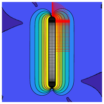
(a) Direct quadrature error

tolerance

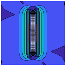
(b) Special quadrature error,

tolerance ${10}^{-6}$

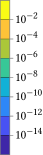
(c)

tolerance

Figure 11: Error in a slice through the rod particle, when evaluating the stresslet identity (3) in free space using (a) direct quadrature, and (b) combined special quadrature with tolerance ${10}^{-6}$. In (b), the tolerance is exceeded in 148 points, marked red; the evaluation grid consists of $500\times 500$ points and the largest error is $1.455\text{\times}{10}^{-6}$. In (a), the 65 lines used to select parameters are shown in red.

Applying the same constant density $\tilde{\boldsymbol{q}}=(1,1,1)/\sqrt{3}$, the direct quadrature error is shown in Figure 11 (a). The special quadrature parameters are selected as described in section 2, with the error along the 65 lines shown in red in Figure 11 (a) used to select the threshold distances. The parameters for error tolerance ${10}^{-6}$ are

$$\begin{array}[]{r@{\:}c@{\:}l@{\qquad}r@{\:}c@{\:}l@{\qquad}r@{\:}c@{\:}l}r_{\text{QBX}}/h\>&=\hfil\>&1,&N_{\text{U}}\>&=\hfil\>&2,\\ d_{\text{QBX}}\>&=\hfil\>&0.234,&d_{\text{U1}}\>&=\hfil\>&0.930,&\kappa_{\text{U1}}\>&=\hfil\>&2,\\ p_{\text{QBX}}\>&=\hfil\>&28,&d_{\text{U2}}\>&=\hfil\>&0.355,&\kappa_{\text{U2}}\>&=\hfil\>&3.\\ \kappa_{\text{QBX}}\>&=\hfil\>&20,\\ \end{array}$$ (7)

The error when using these parameters is shown in Figure 11 (b). As before, the tolerance is not strictly enforced, but the error stays within a factor 2 of the tolerance.

The parameters (7) for the slender rod can be compared with the parameters (6) for the less slender rod with the same tolerance; the threshold distances are relative to the diameter of the cylindrical part of the rod in both cases. Note that the slender rod (7) has larger threshold distances than the other rod (6). This reflects the fact that the error of the underlying direct quadrature at a fixed distance from the rod is higher for the slender rod, since it has lower overall resolution (grid points per surface area). The slender rod also requires a higher $p_{\text{QBX}}$ since $r_{\text{QBX}}=h$ is larger for the slender rod.

4 Example III: a pair of plane walls

In this third example, we select parameters for a plane wall. Since we always consider walls in a periodic setting, we will do so here as well, and use the Spectral Ewald (SE) method described in section 4. We will here select the SE parameters such that the error from SE is completely negligible compared to the quadrature errors which we strive to control here. Since the problem is periodic in all three spatial directions, we must have a pair of walls so that the fluid domain can be confined between them. The periodic cell is here of size $\boldsymbol{B}=(1,1,1)$ and the two walls are placed at a distance of 0.6 from each other. The walls are discretized using $11\times 11$ patches each, with $8\times 8$ grid points on each patch (as described in section 2), in total 7744 grid points per wall. For a wall, we define the grid spacing as $h=\max(h_{1},h_{2})$, where $h_{1}$ and $h_{2}$ are the largest spacings between grid points in each of the two tensorial directions of the patches. The walls considered here have grid spacing $h\approx 0.01668$. The constant density $\tilde{\boldsymbol{q}}=(0,0,1)$ is applied in the direction of the normal of the lower wall (pointing into the fluid domain). The direct quadrature error is shown in Figure 12 (a).

We follow the procedure in section 2. The threshold distances of the upsampled quadrature regions are computed by evaluating the stresslet identity error along normal lines of the walls, with each line centred at a grid point. The error is plotted in Figure 12 (b), and the resulting threshold distances for error tolerance ${10}^{-6}$ are $d_{\text{U1}}=0.0687$, $d_{\text{U2}}=0.0304$ and $d_{\text{QBX}}=0.0198$.

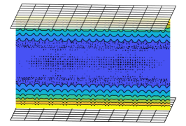
(a) Direct quadrature error

(c)

(b) Upsampled quadrature error

Figure 12: Errors when evaluating the stresslet identity (3) in the periodic setting. (a) Error in the centre plane for direct quadrature. (b) Largest error for upsampled quadrature with different upsampling factors $\kappa$, as a function of the distance to the lower wall.

To determine $p_{\text{QBX}}$ and $\kappa_{\text{QBX}}$, we do a parameter study, shown in Figure 13 (a). Note that the plane wall needs a significantly lower $p_{\text{QBX}}$ than the rod particles to reach a given error. The error curves in Figure 13 (a) level out at around ${10}^{-12}$ due to other errors not controlled by the QBX parameters. In order to reach the tolerance ${10}^{-6}$ it is sufficient to choose $p_{\text{QBX}}=7$ and $\kappa_{\text{QBX}}=10$. The selected parameters are thus

$$\begin{array}[]{r@{\:}c@{\:}l@{\qquad}r@{\:}c@{\:}l@{\qquad}r@{\:}c@{\:}l}r_{\text{QBX}}/h\>&=\hfil\>&1,&N_{\text{U}}\>&=\hfil\>&2,\\ d_{\text{QBX}}\>&=\hfil\>&0.0198,&d_{\text{U1}}\>&=\hfil\>&0.0687,&\kappa_{\text{U1}}\>&=\hfil\>&2,\\ p_{\text{QBX}}\>&=\hfil\>&7,&d_{\text{U2}}\>&=\hfil\>&0.0304,&\kappa_{\text{U2}}\>&=\hfil\>&3.\\ \kappa_{\text{QBX}}\>&=\hfil\>&10,\\ \end{array}$$ (8)

The error when using these parameters is shown in Figure 13 (b).

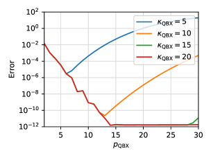
(a) Onsurface QBX error for different $\kappa_{\text{QBX}}$

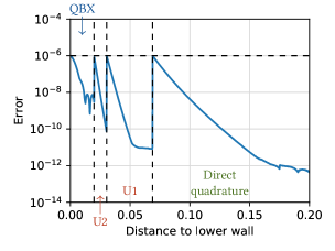
(b) Special quadrature error, tolerance ${10}^{-6}$

Figure 13: (a) Maximal onsurface error when evaluating the stresslet identity using QBX, for different $\kappa_{\text{QBX}}$ with $r_{\text{QBX}}/h=1$ fixed. (b) Maximal stresslet identity error as a function of the distance to the lower wall (for 1000 equispaced distances in $[0,0.2]$), using the combined special quadrature with tolerance ${10}^{-6}$. The largest error is $9.812\text{\times}{10}^{-7}$.

Chapter 6 Numerical results

Our numerical method can be summarized as follows:

1. The geometry is discretized as in section 2. Parameters for the combined special quadrature method are selected as in section 2. Parameter selection is done in free space for particles, but the same parameters can also be used in the periodic setting. For walls, parameter selection is done in the periodic setting.

2. The matrices $\boldsymbol{M}_{i}$ and $\boldsymbol{R}_{i}$ for offsurface QBX and onsurface QBX, respectively, are precomputed as in section 3. Interpolation matrices for the upsampled quadrature regions are also precomputed. At this point, the special quadrature is ready to be used to evaluate the layer potential.

3. The boundary integral equation for either a resistance problem or a mobility problem is solved iteratively for $\boldsymbol{q}$ using GMRES. The Spectral Ewald method is used for periodic problems, as described in section 4. A preconditioner is used in all cases, as described below.

   • For a resistance problem, velocities are given for all particles and the boundary integral equation is given by equation (4).

   • For a mobility problem, forces and torques are applied to all particles and the boundary integral equation is given by equation (5).

4. The flow field in the fluid domain may be computed in a postprocessing step using $\boldsymbol{q}$ from step 3. For a resistance problem, the forces and torques acting on all particles may also be computed here, while for a mobility problem, the particle velocities may be computed.

To improve the convergence of GMRES in step 3, we use a block-diagonal preconditioner similar to the one used in [25]. The preconditioner is constructed by computing the explicit inverse of a single-particle system as well as a system consisting of a single wall patch (if walls are present in the simulation). These two types of blocks are then placed along the diagonal and rotated according to the geometry. This preconditioner has been seen to reduce the number of GMRES iterations by as much as a factor 17 for some systems with many particles, such as the ones in section 3.

In this section, we test some aspects of our numerical method, with focus on the special quadrature. First, in section 1, we test the quadrature on its own (i.e. steps 1–2 above) with geometries containing both particles and walls. This serves as a continuation of the tests in section 5, where geometrical objects were considered only separately. In section 2, we test the special quadrature in the context of the full numerical method (steps 1–4 above) and in particular how the quadrature tolerance influences the accuracy. Finally, in section 3, we test the computational complexity of the method on a more complicated problem, and compute streamlines.

1 Special quadrature with composite geometries

We consider two geometrical setups, shown in Figures 1 and 3. Both problems are periodic with a periodic cell of size $\boldsymbol{B}=(1,1,1)$, and the Spectral Ewald parameters are as in section 4. As in section 5, we use the stresslet identity (3) to estimate the error. This is the same test used to select the parameters, so it mainly serves as a consistency check (tests with nonconstant densities will follow in section 2).

1 Geometry 1: Two rods between a pair of plane walls

The first geometry consists of two plane walls discretized as in section 4, at a distance 0.6 from each other. Between these walls are two rod particles of length $L=0.5$ and radius $R=L/20$ (aspect ratio 10), discretized as in section 3 (but scaled down a factor 20), oriented such that their axes lie in the centre plane.

The stresslet identity error is shown for two different quadrature tolerances $\varepsilon_{\text{tol}}$ in Figure 1. In (a), $\varepsilon_{\text{tol}}=${10}^{-6}$$, the quadrature parameters for the walls are as in section 4, i.e. given by (8); for the rods, the parameters are as in section 3 but with all distances scaled by $1/20$ to account for the difference in size. Thus, the parameters for $\varepsilon_{\text{tol}}=${10}^{-6}$$ for the rods are $d_{\text{QBX}}=0.0117$, $p_{\text{QBX}}=28$, $\kappa_{\text{QBX}}=20$ and $N_{\text{U}}=2$, $d_{\text{U1}}=0.0465$, $d_{\text{U2}}=0.0178$. In (b), for tolerance $\varepsilon_{\text{tol}}=${10}^{-8}$$, the parameters selected according to section 2 are, for the walls $d_{\text{QBX}}=0.0248$, $p_{\text{QBX}}=10$, $\kappa_{\text{QBX}}=10$ and $N_{\text{U}}=2$, $d_{\text{U1}}=0.0944$, $d_{\text{U2}}=0.0386$; and for the rods $d_{\text{QBX}}=0.0146$, $p_{\text{QBX}}=40$, $\kappa_{\text{QBX}}=25$ and $N_{\text{U}}=2$, $d_{\text{U1}}=0.0676$, $d_{\text{U2}}=0.0237$. The maximal error in the centre plane is plotted for varying quadrature tolerance in Figure 2. This shows that the error more or less follows the tolerance, as expected.

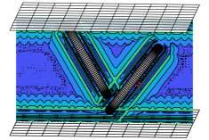
(a) Special quadrature error, tolerance ${10}^{-6}$

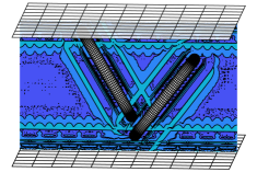
(b) Special quadrature error, tolerance ${10}^{-8}$

(c)

Figure 1: Stresslet identity error in the centre plane, for geometry 1, in (a) for tolerance ${10}^{-6}$ and in (b) for tolerance ${10}^{-8}$. The largest error is $1.205\text{\times}{10}^{-6}$ in (a) and $9.389\text{\times}{10}^{-9}$ in (b). In (a), the error exceeds the tolerance in 2 points (the evaluation grid has $500\times 500$ points), marked red.

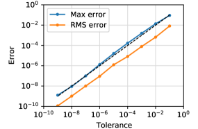
Figure 2: Maximal and root-mean-square (RMS) stresslet identity error in the centre plane as a function of the special quadrature tolerance, for geometry 1. As observed already in section 5, the tolerance is sometimes exceeded slightly at the threshold distances, which causes the max error curve to lie above the identity line Error = Tolerance (dashed).

2 Geometry 2: Two spheroids in a pipe

The second geometry consists of a pipe of radius 0.3, discretized using $5\times 10$ patches with $6\times 6$ grid points each. Inside the pipe are two spheroids with semiaxes $a=0.05$ and $c=0.1$, discretized with parameters $n_{\theta}=36$ and $n_{\varphi}=25$ (900 grid points per spheroid).

We select the error tolerance $\varepsilon_{\text{tol}}=${10}^{-6}$$. The parameters selected according to section 2 are, for the pipe $d_{\text{QBX}}=0.0614$, $p_{\text{QBX}}=12$, $\kappa_{\text{QBX}}=10$ and $N_{\text{U}}=2$, $d_{\text{U1}}=0.222$, $d_{\text{U2}}=0.0888$; and for the spheroids $d_{\text{QBX}}=0.0153$, $p_{\text{QBX}}=27$, $\kappa_{\text{QBX}}=15$ and $N_{\text{U}}=2$, $d_{\text{U1}}=0.0568$, $d_{\text{U2}}=0.0235$. The error when using these parameters is shown in Figure 3 (b), together with the direct quadrature error in Figure 3 (a). Note that we have selected a much lower resolution for the pipe in comparison to the walls in geometry 1 (section 1), which is reflected in the larger threshold distances compared to (8).

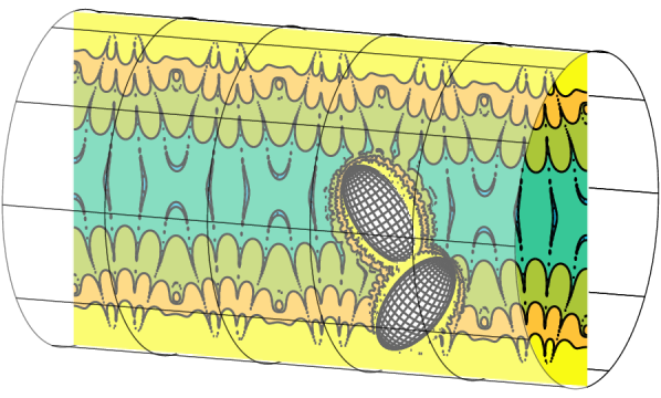
(a) Direct quadrature error

tolerance

.

(b) Special quadrature error,

tolerance ${10}^{-6}$

Upq

(c)

Figure 3: Stresslet identity error in the centre plane, for geometry 2, in (a) using direct quadrature and in (b) using combined special quadrature with tolerance ${10}^{-6}$. In (b), the tolerance is exceeded in 5 points (the evaluation grid has $500\times 500$ points), marked red; the largest error in the slice is $1.323\text{\times}{10}^{-6}$.

2 Solving the boundary integral equation

Here, we investigate how the special quadrature tolerance influences the accuracy of the numerical method, i.e. when solving the boundary integral equation. We will use the mobility problem as our model problem, and apply the force $\boldsymbol{F}=(0,0,-1)$ to all particles, with zero torque and no background flow. In order to get the expected accuracy when solving the boundary integral equation, the double layer density must be well-resolved by the geometry discretization. It turns out that for elongated particles, the density and how easy it is to resolve depends heavily on the number of completion sources $N_{\text{src}}$ (defined in section 1). Therefore, we begin in section 1 by investigating how large $N_{\text{src}}$ must be to ensure that the density is well-resolved for a given discretization. Then, in section 2, we study how the special quadrature tolerance influences the accuracy of the method.

1 Selecting the number of completion sources

To study the influence of $N_{\text{src}}$, we consider a single rod particle with length $L=0.5$ and radius $R=L/20$ (aspect ratio 10) in free space, shown in Figure 5 (a) together with the flow field resulting from the force $\boldsymbol{F}=(0,0,-1)$. We now solve this mobility problem for varying $N_{\text{src}}$, with the special quadrature error tolerance fixed to ${10}^{-9}$ here.

The completion flow $\boldsymbol{\mathcal{V}}^{(\alpha)}$, which appears in the right-hand side of the boundary integral equation (18), will change drastically as $N_{\text{src}}$ grows from small values, as shown in Figure 4; the completion flow becomes increasingly smoother as $N_{\text{src}}$ increases. Naturally, this means that the density $\boldsymbol{q}$ itself will change as $N_{\text{src}}$ grows. However, the real physical quantities – the particle velocity and the flow field – should not change since the net force and torque on the particle does not change. Thus, these physical quantities can be used to gauge how $N_{\text{src}}$ affects the accuracy of the solution. As Figure 5 (b) shows, the effect is quite large, and most pronounced in the fluid flow velocity (the blue curve). (For this problem, the magnitude of the fluid flow velocity and particle velocity $\boldsymbol{U}_{\text{RBM}}$ are both around 0.6, while the angular velocity $\boldsymbol{\Omega}_{\text{RBM}}$ is zero.)

Thus, it is important to select $N_{\text{src}}$ high enough for the error in Figure 5 (b) to satisfy the error tolerance. The effect of $N_{\text{src}}$ on the accuracy is stronger the more elongated the particle is; for particles with low aspect ratio, $N_{\text{src}}=1$ may be sufficient. The effect is very similar for the resistance problem, to the degree that the max flow error in Figure 5 (b) can be used to determine $N_{\text{src}}$ for both the mobility problem and resistance problem. Note that $N_{\text{src}}$ does not affect the size of the linear system, i.e. (4) or (5).

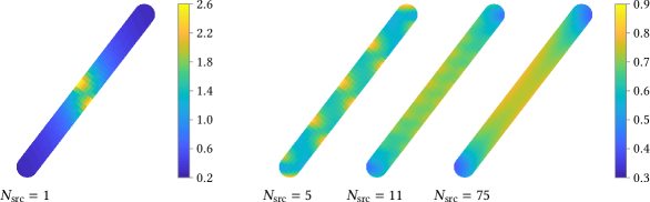
Figure 4: The magnitude of the completion flow $\boldsymbol{\mathcal{V}}^{(\alpha=1)}[\boldsymbol{F},\boldsymbol{0}](\boldsymbol{x})$ on the surface of the rod, for a few different values of $N_{\text{src}}$. Since the background flow is zero, this is exactly the right-hand side of the boundary integral equation (18). Note that the colour scale is different for $N_{\text{src}}=1$ compared to the other values.

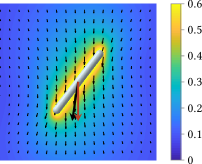
(a) Flow field

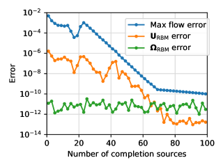
(b) Error contribution

Figure 5: (a) Flow field resulting from the mobility problem for a single rod in free space (colour indicates velocity magnitude, small black arrows indicate velocity direction). The large red arrow indicates the applied force, and the large black arrow indicates the velocity of the rod (not to scale with the small arrows). (b) Contribution to the absolute error from the way the completion sources are distributed, as a function of $N_{\text{src}}$ (for a rod particle of aspect ratio 10). The error is estimated as the difference to a reference solution with $N_{\text{src}}=135$. Note that the max flow error flattens out around ${10}^{-9}$, the special quadrature error tolerance.

2 Effect of the special quadrature on the accuracy

We continue to study the mobility problem, but now add another rod particle and a pair of plane walls, as shown in Figure 6. We fix $N_{\text{src}}=65$, which was enough to get the error below ${10}^{-9}$ in the previous problem. The walls are discretized using $22\times 22$ patches with $8\times 8$ grid points each (30 976 grid points per wall), and the rod particles are discretized as in section 1. We set the special quadrature tolerance to different values between ${10}^{-1}$ and ${10}^{-8}$, solve the mobility problem, and compute the flow field and particle velocities. The errors in the flow field, density and particle velocities are estimated using a reference solution with special quadrature tolerance ${10}^{-9}$; these are shown in Figures 6 (b) and 7 (a)–(b). Note that the tolerance sets the flow field error relative to $\max\,\lvert\boldsymbol{q}\rvert$ quite accurately; the density and particle velocity errors are even smaller. We would like to point out that the value of the scale factor $\max\,\lvert\boldsymbol{q}\rvert$ is not known a priori, but it is of course known after having solved the boundary integral equation.

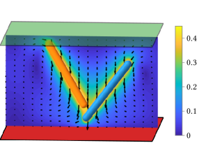
(a) Geometry and flow field

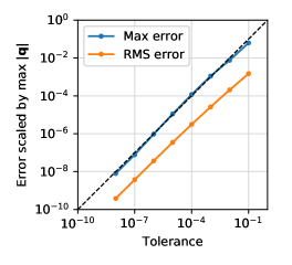
(b) Flow field error

Figure 6: (a) Flow field from the periodic mobility problem with force $\boldsymbol{F}=(0,0,-1)$ applied to both particles (colour indicates velocity magnitude, arrows indicate velocity direction). (b) Maximal and root-mean-square (RMS) flow field error in the centre plane (estimated using a reference solution with tolerance ${10}^{-9}$), scaled by the maximal density magnitude $\max\,\lvert\boldsymbol{q}\rvert\approx 5.4$. The dashed line indicates Scaled error = Tolerance.

It should be noted that the error cannot be expected to follow the tolerance unless the density is well-resolved by the geometry discretization, since otherwise the interpolated density will be inaccurate. It has been observed that the density becomes hard to resolve, with either sharp peaks or high-frequency oscillations, when particles come very close to each other or the walls (where “very close” is measured relative to the grid resolution). Thus, one may be forced to increase the grid resolution in these cases.

For elongated particles, the set of matrices $\boldsymbol{M}_{i}$, $i=1,\ldots,n_{\theta}/2$, which are precomputed for offsurface QBX tends to become quite large for strict quadrature tolerances. The reason for this is that with particle-global QBX, the whole set of matrices consists of

$$3n_{\varphi}n_{\theta}^{2}(p_{\text{QBX}}+1)(p_{\text{QBX}}+2)$$ (1)

complex numbers, i.e. it is quadratic in both $p_{\text{QBX}}$ and $n_{\theta}$ (where $n_{\theta}$ is the number of grid points in the axial direction, which we define as $2n_{1}+n_{2}$ for rod particles). For elongated particles, $n_{\theta}$ tends to be large; for example, for the rods considered in this section (aspect ratio 10), $n_{\theta}=130$ and $n_{\varphi}=18$. The set of matrices for tolerance ${10}^{-8}$ ($p_{\text{QBX}}=40$) then takes up around 25 gigabytes when stored in double precision, while for tolerance ${10}^{-6}$ ($p_{\text{QBX}}=28$) the matrices take up around 13 gigabytes. To reduce the size of the matrices in this situation, a local patch-based discretization could be used also for the particles, in the same way it is already used for the walls. This would reduce the number of grid points included in the special quadrature and thus the size of the matrices.

3 Computational complexity and computation of streamlines

1 Computational complexity of the method

The computational cost of our special quadrature method is quadratic in the number of grid points per particle (or patch), but linear in the number of particles (patches) if their discretization is kept fixed. For the Spectral Ewald method, the computational cost scales like $O(N\log N)$, where $N$ is the number of unknowns in the system (i.e. three times the total number of grid points), assuming that the number of grid points within a ball of radius $r_{\text{c}}$ does not change. In other words, for fixed grid resolution and particle concentration, the time required per GMRES iteration when solving the boundary integral equation is expected to scale like $O(N\log N)$.

To test this scaling, we consider a problem with many rod particles confined in a pipe, shown in Figure 8: one segment (a) consists of a pipe segment of radius 0.3 and length 0.2 confined in a periodic cell of size $\boldsymbol{B}=(0.2,1,1)$, with 20 rods of length $L=0.25$ and radius $R=L/12$ (aspect ratio 6) inside the pipe. This segment is replicated to create a longer pipe, up to 12 times the original length (shown in (b)), with the same grid point concentration as the original segment. For $1,2,3,\ldots,12$ segments, we solve a resistance problem in which all particles are stationary and a quadratic background flow

$$\boldsymbol{u}_{\text{bg}}(\boldsymbol{x})=\left(\frac{A^{2}-x_{2}^{2}-x_{3}^{2}}{A^{2}},\hskip 5.0pt0,\hskip 5.0pt0\right)$$ (2)

is applied, where $A=0.3$ is the radius of the pipe and $(x_{2},x_{3})=(0,0)$ is its centre line.

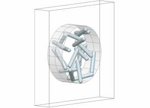
(a) 1 segment

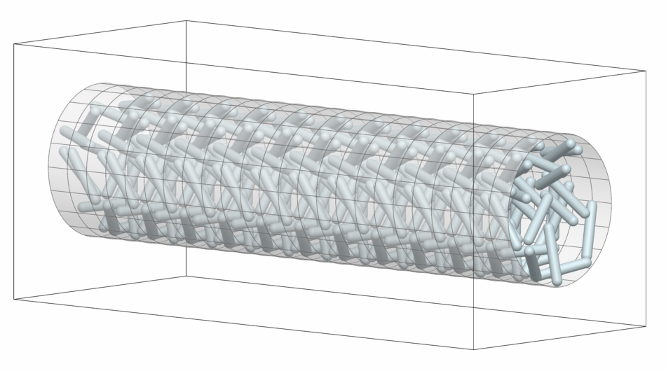
(b) 12 segments

Figure 8: The geometry in section 1 is made up of stacked identical segments, where each segment contains 20 rods and $2\times 20$ pipe patches. In total, there are 27 360 grid points and 82 080 unknowns in each segment.

As seen in Figure 9 (a), the time per GMRES iteration follows the expected scaling $O(N\log N)$. Since the structure of the linear system changes as the number of segments $n_{\text{s}}$ grows, the number of GMRES iterations grows slightly with $n_{\text{s}}$. However, this growth is slow enough for the total solving time to also follow the scaling $O(N\log N)$, as shown in Figure 9 (b).

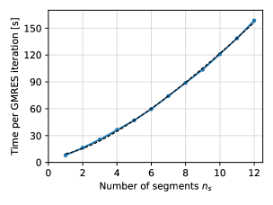
(a) Time per GMRES iteration

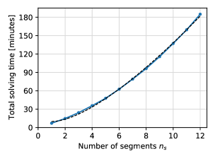
(b) Total solving time

Figure 9: Time required to solve the resistance problem for the geometry in Figure 8 with GMRES tolerance ${10}^{-6}$ in MATLAB, (a) per GMRES iteration and (b) in total. With 82 080 unknowns per segment, the number of unknowns ranges from 82 080 to 984 960. The dashed curves are least-squares fits of $T=A\,n_{\text{s}}\log n_{\text{s}}+B\,n_{\text{s}}+C$ to the data, where $n_{\text{s}}$ is the number of segments. In (a), $A=5.8$, $B=-2.4$, $C=12.2$ (seconds), and in (b), $A=9.0$, $B=-8.7$, $C=18.6$ (minutes). Thus, the time scales as $O(n_{\text{s}}\log n_{\text{s}})$.

2 Streamline computation

In the postprocessing step (step 4 of the method summary), streamlines may be computed to visualize the flow field. When using the Spectral Ewald method, the Fourier-space part on the uniform grid can be reused to reduce the computation time, as described in appendix D. Here, we compute streamlines for a periodic resistance problem with 100 rods in a pipe segment of length 1, otherwise identical to the problem in section 1 (including all parameters). Figure 10 shows 95 streamlines; a typical streamline consists of around 3000 points and takes around 2 minutes to compute (i.e. around 0.04 seconds per time step). A slice of the same flow field is shown in Figure 11.

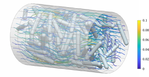
Figure 10: Streamlines for the resistance problem (colour indicate velocity magnitude).

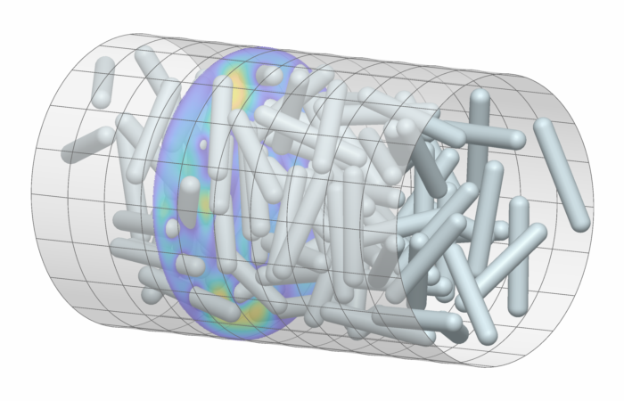
Streamwise velocity

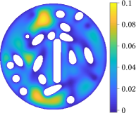
Transverse velocity

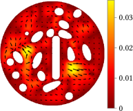
Figure 11: Flow field shown in a slice at streamwise position $x=2/3$.

Chapter 7 Effects of nonsmooth geometries

So far, all geometrical objects considered in this paper have been smooth. In fact, special care has been taken to ensure that the rod particles, constructed in appendix B, are everywhere smooth. The reason is that, as noted in [14], the convergence of the local expansions used in QBX depends on the smoothness of the boundary close to the expansion centre. In this section, we demonstrate this using two different rod particles: one smooth and one nonsmooth, shown in Figure 1 (a). The rods are both of length $L$ and radius $R$, but the smooth rod is constructed as in appendix B, while the nonsmooth rod consists of a cylinder of radius $R$ and length $L-2R$ joined to two half-spherical caps of radius $R$. The nonsmooth rod is thus of class $C^{1}$, since the curvature is discontinuous where the cylinder meets the spherical caps.

To illustrate the convergence of QBX, consider rods with $L/R=20$ (aspect ratio 10), discretized using $n_{1}=35$, $n_{2}=60$, $n_{\varphi}=18$ as described in section 1. In Figure 1 (b), the onsurface QBX stresslet identity error is plotted as a function of $p_{\text{QBX}}$, in the same way as in section 3 (where this was done for the smooth rod). Clearly, the convergence with respect to $p_{\text{QBX}}$ is much worse for the nonsmooth rod compared to the smooth one. The reason for this can be seen in Figure 2: the error decays extremely slowly close to the boundary between the cylinder and the caps, where the curvature is discontinuous. This is clearly a local effect, since the convergence is fine a little bit away from the discontinuity.

It should be noted that it is entirely possible to use QBX on a nonsmooth geometry, but it requires special measures to be taken. In [29], QBX was applied to a geometry with a corner. In that example, the discretization was dyadically refined around the corner, to ensure that the layer potential appears locally smooth on the scale of the discretization. The same approach could likely be taken also for the nonsmooth rod particle, i.e. refining the grid dyadically around the discontinuity. However, constructing the rod to be smooth in the first place has a clear advantage in this case, since no grid refinement is needed.

(a) Geometries

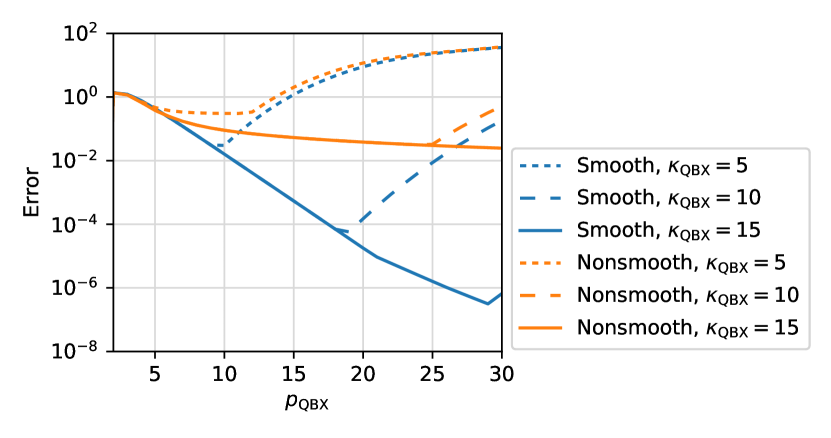
(b) QBX onsurface error

Figure 1: (a) A smooth and a nonsmooth rod, both of length $L$ and radius $R$. Note that each cap of the smooth rod (marked with red lines) has length $1.5R$, while each cap of the nonsmooth rod has length $R$. (b) Maximal onsurface QBX stresslet identity error for the smooth and nonsmooth rod, with expansion radius $r_{\text{QBX}}=h=2\pi R/n_{\varphi}$ fixed.

Figure 2: (a) The QBX stresslet identity error shown in a slice through selected balls of convergence, for $r_{\text{QBX}}=h$, $p_{\text{QBX}}=25$ and $\kappa_{\text{QBX}}=15$. (b) The onsurface QBX error on the rods, with the same parameters as in (a).

Chapter 8 Conclusions

We have presented a numerical method based on a boundary integral formulation that can be used to simulate rigid particles in Stokes flow with confining walls. A parameter selection strategy has also been presented for the combined special quadrature used in this method. We have demonstrated that the error of the method is controlled by the special quadrature tolerance as long as the layer density is well-resolved, and that the method scales as $O(N\log N)$ in the number of unknowns $N$ for fixed grid point concentration. This makes it possible to simulate systems with a large number of particles. The method can deal with particles and walls of different shapes; we have here considered spheroids, rod particles, pipes and plane walls, but it is straightforward to extend the method to any smooth geometry with sufficient symmetry.

The method could be further improved for example by using local patch-based quadrature for elongated particles to reduce the size of the QBX matrices, and allowing the size of the wall patches to be set adaptively so that the resolution can be focused where particles are close to the wall. It could also be useful to allow parameters such as $p_{\text{QBX}}$ to vary along the particle surface (in response to differences in the convergence rate of the local expansions, as seen e.g. in Figure 2), and to allow the expansion centres for QBX to be placed independently of the grid points of the discretization, so that the centres can be placed closer to the surface in order to decrease the expansion order $p_{\text{QBX}}$. Furthermore, if analytical quadrature error estimates were available, these could replace the numerical experiments used to select threshold distances and the QBX upsampling factor.

Appendix A The stresslet identity for plane walls and pipes

Here we show that a variant of the stresslet identity (3) holds for a pair of parallel infinite plane walls (in section 1) and an infinitely long pipe (in section 2).

1 A pair of parallel plane walls

Let $\Gamma_{1}$ and $\Gamma_{2}$ be two parallel infinite planes oriented as shown in Figure 1, one wall placed at $x_{3}=a$ and the other at $x_{3}=-a$ for some $a>0$. Let the domain between the two walls (which we will think of as the fluid domain) be denoted by $\Omega$.

Figure 1: Two parallel infinite planes $\Gamma_{1}$ and $\Gamma_{2}$.

Let $\tilde{\Gamma}=\Gamma_{1}\cup\Gamma_{2}$, and let $\tilde{\boldsymbol{q}}\in\mathbb{R}^{3}$ be any constant vector. We shall show that

$$\boldsymbol{\mathcal{D}}[\tilde{\Gamma},\tilde{\boldsymbol{q}}](\boldsymbol{x})=\begin{cases}-8\pi\tilde{\boldsymbol{q}},&\text{if $\boldsymbol{x}\in\Omega$},\\ -4\pi\tilde{\boldsymbol{q}},&\text{if $\boldsymbol{x}\in\tilde{\Gamma}$},\\ \boldsymbol{0},&\text{otherwise},\\ \end{cases}$$ (1)

where the double layer potential $\boldsymbol{\mathcal{D}}$ is given by (1).

Since $\tilde{\boldsymbol{q}}$ is constant and the normals are given by $\boldsymbol{n}^{1}=(0,0,-1)$ and $\boldsymbol{n}^{2}=(0,0,1)$, we can write

$$\mathcal{D}_{i}[\tilde{\Gamma},\tilde{\boldsymbol{q}}](\boldsymbol{x}) =\tilde{q}_{j}\int_{\tilde{\Gamma}}T_{ijk}(\boldsymbol{x}-\boldsymbol{y})n_{k}(\boldsymbol{y})\,\mathrm{d}S(\boldsymbol{y})$$ (2)

$$=-\tilde{q}_{j}\underbrace{\int_{\Gamma_{1}}T_{ij3}(\boldsymbol{x}-\boldsymbol{y})\,\mathrm{d}S(\boldsymbol{y})}_{J^{1}_{ij}(\boldsymbol{x})}\>+\>\tilde{q}_{j}\underbrace{\int_{\Gamma_{2}}T_{ij3}(\boldsymbol{x}-\boldsymbol{y})\,\mathrm{d}S(\boldsymbol{y})}_{J^{2}_{ij}(\boldsymbol{x})}.$$ (3)

The two integrals which we have called $J^{1}_{ij}$ and $J^{2}_{ij}$ can both be expressed in terms of the integral

$$J^{0}_{ij}(\boldsymbol{x})=\int_{\Gamma_{0}}T_{ij3}(\boldsymbol{x}-\boldsymbol{y})\,\mathrm{d}S(\boldsymbol{y}),$$ (4)

where $\Gamma_{0}=\{\boldsymbol{x}\in\mathbb{R}^{3}:x_{3}=0\}$. The integrals are related through $J^{0}_{ij}(\boldsymbol{x})=J^{1}_{ij}(\boldsymbol{x}+a\boldsymbol{e}_{3})=J^{2}_{ij}(\boldsymbol{x}-a\boldsymbol{e}_{3})$, with $\boldsymbol{e}_{3}=(0,0,1)$. In fact, since $\Gamma_{0}$ is infinite, the integral $J^{0}_{ij}(\boldsymbol{x})$ as given by (4) depends only on $x_{3}$, i.e.

$$J^{0}_{ij}(\boldsymbol{x})=J^{0}_{ij}(x_{3})=\int_{\Gamma_{0}}T_{ij3}(x_{3}\boldsymbol{e}_{3}-\boldsymbol{y})\,\mathrm{d}S(\boldsymbol{y}).$$ (5)

Inserting the expression for the stresslet $\boldsymbol{T}$ from (1) into (5), we find

$$J^{0}_{ij}(x_{3})=-6x_{3}\int_{-\infty}^{\infty}\int_{-\infty}^{\infty}\frac{(x_{3}\delta_{i3}-y_{i})(x_{3}\delta_{j3}-y_{j})}{(y_{1}^{2}+y_{2}^{2}+x_{3}^{2})^{5/2}}\mathrm{d}y_{1}\mathrm{d}y_{2},$$ (6)

where $y_{3}=0$. This double integral can be computed analytically, and the result is

$$J^{0}_{ij}(x_{3})=-4\pi\operatorname{sgn}(x_{3})\delta_{ij},$$ (7)

where $\operatorname{sgn}(\cdot)$ denotes the sign function. Using the relations $J^{1}_{ij}(\boldsymbol{x})=J^{0}_{ij}(x_{3}-a)$ and $J^{2}_{ij}(\boldsymbol{x})=J^{0}_{ij}(x_{3}+a)$ and inserting (7) into (3), we get

$$\mathcal{D}_{i}[\tilde{\Gamma},\tilde{\boldsymbol{q}}](\boldsymbol{x})=4\pi\tilde{q}_{i}\operatorname{sgn}(x_{3}-a)-4\pi\tilde{q}_{i}\operatorname{sgn}(x_{3}+a).$$ (8)

From this the result (1) follows.

2 A pipe

Let now $\tilde{\Gamma}$ be an infinitely long pipe given by the equation $x_{2}^{2}+x_{3}^{2}=a^{2}$ for some $a>0$, as shown in Figure 2. Let the domain inside the pipe be denoted by $\Omega$. We shall show that for any constant vector $\tilde{\boldsymbol{q}}\in\mathbb{R}^{3}$, the identity (1) holds.

Figure 2: An infinite cylindrical pipe $\tilde{\Gamma}$.

Let us introduce cylindrical coordinates and write $\boldsymbol{x}=x_{1}\boldsymbol{e}_{1}+r\boldsymbol{e}_{\varphi}$ and $\boldsymbol{y}=y_{1}\boldsymbol{e}_{1}+a\boldsymbol{e}_{\theta}$ for the evaluation point and integration variable, respectively. The unit vectors are given by

$$\boldsymbol{e}_{1}=(1,0,0),\qquad\boldsymbol{e}_{\varphi}=(0,\cos\varphi,\sin\varphi)\qquad\text{and}\qquad\boldsymbol{e}_{\theta}=(0,\cos\theta,\sin\theta),$$ (9)

and $r\geq 0$. Using the fact that the normal vector is given by $\boldsymbol{n}(\boldsymbol{y})=-\boldsymbol{e}_{\theta}$, we can write the double layer potential from (1) as

$$\mathcal{D}_{i}[\tilde{\Gamma},\tilde{\boldsymbol{q}}](\boldsymbol{x})=-\tilde{q}_{j}\int_{0}^{2\pi}\int_{-\infty}^{\infty}T_{ijk}(x_{1}\boldsymbol{e}_{1}+r\boldsymbol{e}_{\varphi}-y_{1}\boldsymbol{e}_{1}-a\boldsymbol{e}_{\theta})(\boldsymbol{e}_{\theta})_{k}\,a\,\mathrm{d}y_{1}\mathrm{d}\theta,$$ (10)

where $(\boldsymbol{e}_{\theta})_{k}$ denotes the $k$th component of $\boldsymbol{e}_{\theta}$. Using the variable substitution $y_{1}-x_{1}=u$, we can eliminate $x_{1}$. Writing out the stresslet $\boldsymbol{T}$ from (1), and using a few trigonometric identities, the integral in (10) can be written as

$$\mathcal{D}_{i}[\tilde{\Gamma},\tilde{\boldsymbol{q}}](\boldsymbol{x})=6\tilde{q}_{j}a\underbrace{\int_{0}^{2\pi}\int_{-\infty}^{\infty}\frac{(r\boldsymbol{e}_{\varphi}-u\boldsymbol{e}_{1}-a\boldsymbol{e}_{\theta})_{i}(r\boldsymbol{e}_{\varphi}-u\boldsymbol{e}_{1}-a\boldsymbol{e}_{\theta})_{j}(r\cos(\varphi-\theta)-a)}{\,\big{(}u^{2}+r^{2}+a^{2}-2ra\cos(\varphi-\theta)\big{)}^{5/2}}\,\mathrm{d}u\,\mathrm{d}\theta}_{I_{ij}(r,\varphi)}.$$ (11)

At this point it is not immediately apparent that the integral which we have called $I_{ij}(r,\varphi)$ is independent of $\varphi$, but that does indeed turn out to be the case. We expect the offdiagonal elements of $I_{ij}$ to be zero, which can be verified by first integrating in $u$ and then in $\theta$. It thus remains to compute the diagonal elements of $I_{ij}$.

To compute $I_{11}$, first integrate in $u$ using the formula

$$\int_{-\infty}^{\infty}\frac{u^{2}}{(u^{2}+C)^{5/2}}\,\mathrm{d}u=\frac{2}{3C},\qquad C>0.$$ (12)

The outer integral becomes

$$I_{11}(r,\varphi)=\frac{2}{3}\int_{0}^{2\pi}\frac{r\cos(\varphi-\theta)-a}{r^{2}+a^{2}-2ra\cos(\varphi-\theta)}\,\mathrm{d}\theta.$$ (13)

The variable $\varphi$ can now be eliminated using the substitution $\theta-\varphi=\nu$ (and the limits shifted back to $[0,2\pi]$ due to periodicity). The value of the integral can then be calculated to be

$$I_{11}(r,\varphi)=\frac{2\pi}{3a}\,\big{(}\operatorname{sgn}(r-a)-1\big{)},\qquad r\geq 0,$$ (14)

where $\operatorname{sgn}(\cdot)$ is the sign function.

To compute $I_{22}$, first integrate in $u$ using the formula

$$\int_{-\infty}^{\infty}\frac{1}{(u^{2}+C)^{5/2}}\,\mathrm{d}u=\frac{4}{3C^{2}},\qquad C>0,$$ (15)

to get

$$I_{22}(r,\varphi)=\frac{4}{3}\int_{0}^{2\pi}\frac{(r\cos\varphi-a\cos\theta)^{2}\left(r\cos(\varphi-\theta)-a\right)}{(r^{2}+a^{2}-2ra\cos(\varphi-\theta))^{2}}\,\mathrm{d}\theta.$$ (16)

Using the substitution $\theta-\varphi=\nu$ and shifting the limits back to $[0,2\pi]$ yields the integral

$$I_{22}(r,\varphi)=\frac{4}{3}\int_{0}^{2\pi}\frac{(r\cos\varphi-a\cos\nu\cos\varphi+a\sin\nu\sin\varphi)^{2}\left(r\cos\nu-a\right)}{(r^{2}+a^{2}-2ra\cos\nu)^{2}}\,\mathrm{d}\nu,$$ (17)

which we compute by expanding the square in the numerator, thus splitting the integral into six terms, after which each term can be integrated separately. The result is

$$I_{22}(r,\varphi)=\frac{2\pi}{3a}\,\big{(}\operatorname{sgn}(r-a)-1\big{)},\qquad r\geq 0.$$ (18)

Note that the dependence on $\varphi$ disappears when summing the six terms to get the above result.

Finally, to compute $I_{33}$, we again start by integrating in $u$ using (15), after which we use the substitution $\theta-\varphi=\nu$ to get

$$I_{33}(r,\varphi)=\frac{4}{3}\int_{0}^{2\pi}\frac{(r\sin\varphi-a\cos\nu\sin\varphi-a\sin\nu\cos\varphi)^{2}(r\cos\nu-a)}{(r^{2}+a^{2}-2ra\cos\nu)^{2}}\,\mathrm{d}\nu.$$ (19)

Comparing (17) and (19), note that $I_{33}(r,\varphi+\pi/2)=I_{22}(r,\varphi)$. But as we saw in (18), $I_{22}$ does not depend on $\varphi$, so $I_{33}=I_{22}$.

To summarize, we have shown that

$$I_{ij}(r,\varphi)=\frac{2\pi}{3a}\!\,\big{(}\!\operatorname{sgn}(r-a)-1\big{)}\delta_{ij}.$$ (20)

Inserting this into (11), we find that

$$\mathcal{D}_{i}[\tilde{\Gamma},\tilde{\boldsymbol{q}}](\boldsymbol{x})=4\pi\tilde{q}_{i}\!\,\big{(}\!\operatorname{sgn}(r-a)-1\big{)},$$ (21)

from which the result (1) follows for the pipe.

Appendix B Construction of smooth rod particles

In this section, we describe how the rod particles are constructed to ensure that they are smooth everywhere. Recall from section 1 the parametrization

$$\begin{cases}x_{1}=\varrho(\theta;L,R)\cos\varphi,\\ x_{2}=\varrho(\theta;L,R)\sin\varphi,\\ x_{3}=\beta(\theta;L,R),\end{cases}$$ (1)

of the rod, where $\varphi\in[0,2\pi)$ and $\theta\in[0,\pi]$ are parameters, $L$ is the length of the rod and $R$ the radius. The goal here is to derive the shape functions $\varrho(\cdot\,;L,R):[0,\pi]\to[0,R]$ and $\beta(\cdot\,;L,R):[0,\pi]\to[-\tfrac{1}{2}L,\tfrac{1}{2}L]$ so that the rod has the smooth shape shown in Figure 1. The rod consists of three smoothly joined parts: a top cap, corresponding to $\theta\in I_{1}=[0,\pi/3]$; a middle cylinder, corresponding to $\theta\in I_{2}=[\pi/3,2\pi/3]$; and a bottom cap, corresponding to $\theta\in I_{3}=[2\pi/3,\pi]$. Let the length of each cap be $L_{\text{cap}}$, as shown in Figure 1. The ratio $L_{\text{cap}}/R$ determines the aspect ratio of the cap. Here, we fix this ratio by setting $L_{\text{cap}}$ to

$$L_{\text{cap}}=1.5R,$$ (2)

which gives the cap a shape similar to a half-sphere. The length of the middle cylinder is then

$$L_{\text{mid}}=L-3R.$$ (3)

However, note that the derivation below is valid for any value of $L_{\text{cap}}\in(0,L/2)$, with $L_{\text{mid}}=L-2L_{\text{cap}}$.

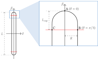
Figure 1: The shape of the smooth rod, here with $L=10$ and $R=0.5$.

Let us for fixed $L$ and $R$ define $\boldsymbol{g}(\theta)=(g_{1}(\theta),g_{2}(\theta))=(\varrho(\theta;L,R),\beta(\theta;L,R))$. For the middle cylinder, the parametrization is

$$g_{1}(\theta)=R,\qquad g_{2}(\theta)=\left(1-\frac{3}{\pi}\theta\right)\!L_{\text{mid}}+\frac{L_{\text{mid}}}{2},\qquad\theta\in I_{2}=[\pi/3,2\pi/3].$$ (4)

Note that $g_{2}$ is simply an affine function of $\theta$. At the endpoints of the interval $I_{2}$ we have

$$\begin{array}[]{r@{\:}c@{\:}l}\boldsymbol{g}(\pi/3)\>&=\hfil\>&(R,L_{\text{mid}}/2),\\[4.0pt] \boldsymbol{g}^{\prime}(\pi/3)\>&=\hfil\>&(0,-(3/\pi)L_{\text{mid}}),\\[4.0pt] \boldsymbol{g}^{(n)}(\pi/3)\>&=\hfil\>&(0,0),\quad n\geq 2,\end{array}\qquad\qquad\text{and}\qquad\qquad\begin{array}[]{r@{\:}c@{\:}l}\boldsymbol{g}(2\pi/3)\>&=\hfil\>&(R,-L_{\text{mid}}/2),\\[4.0pt] \boldsymbol{g}^{\prime}(2\pi/3)\>&=\hfil\>&(0,-(3/\pi)L_{\text{mid}}),\\[4.0pt] \boldsymbol{g}^{(n)}(2\pi/3)\>&=\hfil\>&(0,0),\quad n\geq 2.\end{array}$$ (5)

Our goal is now to extend the parametrization $\boldsymbol{g}(\theta)$ to $I_{1}$ and $I_{3}$ in a way such that the unit tangent vector $\boldsymbol{g}^{\prime}(\theta)/\lvert\boldsymbol{g}^{\prime}(\theta)\rvert$ and its higher derivatives are continuous everywhere. As an intermediate step we introduce an auxiliary function $\widehat{\boldsymbol{g}}(t)=(\widehat{g}_{1}(t),\widehat{g}_{2}(t))$ with a different parameter $t\in[-1,1]$. The function $\widehat{\boldsymbol{g}}$ should trace the curve from C to B via A in Figure 1, with C corresponding to $t=-1$, A corresponding to $t=0$ and B corresponding to $t=1$. We will later relate $t\in[0,1]$ to $\theta\in[0,\pi/3]$ to get the final parametrization. At this point, note that to match (5) we must require

$$\begin{array}[]{r@{\:}c@{\:}l}\widehat{\boldsymbol{g}}(1)\>&=\hfil\>&(R,L_{\text{mid}}/2),\\[4.0pt] \widehat{\boldsymbol{g}}^{\prime}(1)\>&=\hfil\>&(0,-b),\\[4.0pt] \widehat{\boldsymbol{g}}^{(n)}(1)\>&=\hfil\>&(0,0),\quad n\geq 2,\end{array}\qquad\qquad\text{and}\qquad\qquad\begin{array}[]{r@{\:}c@{\:}l}\widehat{\boldsymbol{g}}(-1)\>&=\hfil\>&(-R,L_{\text{mid}}/2),\\[4.0pt] \widehat{\boldsymbol{g}}^{\prime}(-1)\>&=\hfil\>&(0,b),\\[4.0pt] \widehat{\boldsymbol{g}}^{(n)}(-1)\>&=\hfil\>&(0,0),\quad n\geq 2,\end{array}$$ (6)

where $b$ is some positive constant. In order to construct $\widehat{\boldsymbol{g}}(t)$ we will use a bump function $\psi:\mathbb{R}\to\mathbb{R}$, which must satisfy the following:

• $\psi$ must be infinitely differentiable on $\mathbb{R}$,

• $\psi$ must have compact support in $[-1,1]$, i.e. $\psi(t)=0$ if $t>1$ or $t<-1$,

• $\psi(t)$ must be positive for $t\in(-1,1)$,

• $\psi$ must be even, i.e. $\psi(t)=\psi(-t)$ for all $t\in\mathbb{R}$.

We also introduce its primitive function

$$\Psi(t)=\int_{0}^{t}\psi(\tau)\,\mathrm{d}\tau,\qquad t\in\mathbb{R},$$ (7)

which is an odd function since $\psi$ is even. We choose a specific bump function, namely

$$\psi(t)=\begin{cases}\dfrac{(t^{2}+1)\exp[4t/(t^{2}-1)]}{\,\big{[}(t^{2}-1)(1+\exp[4t/(t^{2}-1)])\big{]}^{2}},&\text{if $t\in(-1,1)$},\\[12.0pt] 0,&\text{otherwise}.\end{cases}$$ (8)

This function has the primitive function

$$\Psi(t)=\begin{cases}-\dfrac{1}{8}\tanh\!\left(-\dfrac{2t}{1-t^{2}}\right),&\text{if $t\in(-1,1)$},\\[12.0pt] -\dfrac{1}{8},&\text{if $t\leq-1$},\\[12.0pt] \dfrac{1}{8},&\text{if $t\geq 1$}.\end{cases}$$ (9)

We now construct $\widehat{\boldsymbol{g}}(t)$ as

$$\widehat{g}_{1}(t)=R\frac{\Psi(t)}{\Psi(1)},\qquad\widehat{g}_{2}(t)=\frac{L_{\text{mid}}}{2}-b\int_{-1}^{t}\frac{\Psi(\tau)}{\Psi(1)}\,\mathrm{d}\tau,\qquad t\in[-1,1],$$ (10)

which satisfies (6). We can determine $b$ by noting that we must have $\widehat{g}_{2}(0)=L/2$ (at point A in Figure 1), which yields

$$b=L_{\text{cap}}\frac{\Psi(1)}{\int_{0}^{1}\Psi(\tau)\,\mathrm{d}\tau}.$$ (11)

The integrals of $\Psi$ in (10) and (11) are computed numerically using MATLAB’s integral function.

Finally, we go from the parameter $t$ to the parameter $\theta$. We would like the discretization points to be distributed as Gauss–Legendre points in the arclength, and so we must choose $\theta$ so that it is proportional to the arclength on the caps. Consider the arclength

$$s(t)=\int_{0}^{t}\lvert\widehat{\boldsymbol{g}}^{\prime}(\tau)\rvert\,\mathrm{d}\tau,\qquad t\in[0,1].$$ (12)

Let us then define

$$\theta=G(t)=\frac{\pi}{3}\frac{s(t)}{s(1)},\qquad t\in[0,1],$$ (13)

and note that this defines $\theta\in I_{1}=[0,\pi/3]$ as an invertible function of $t\in[0,1]$. We can now define $\boldsymbol{g}(\theta)=\boldsymbol{g}(G(t))=\widehat{\boldsymbol{g}}(t)$ for $t\in[0,1]$, and thus

$$\boldsymbol{g}(\theta)=\widehat{\boldsymbol{g}}(G^{-1}(\theta)),\qquad\theta\in I_{1}=[0,\pi/3].$$ (14)

The bottom cap should be the reflection of the top cap in the plane corresponding to $\beta=0$, so

$$\boldsymbol{g}(\theta)=(g_{1}(\pi-\theta),-g_{2}(\pi-\theta)),\qquad\theta\in I_{3}=[2\pi/3,\pi].$$ (15)

Now that we have defined $\boldsymbol{g}(\theta)$ for all $\theta\in[0,\pi]$, its two components $g_{1}$ and $g_{2}$ correspond to the shape factors $\varrho(\theta;L,R)$ and $\beta(\theta;L,R)$, respectively, which are to be used in (1).

Appendix C Derivation of the safety factor $\gamma$

Recall from section 5 that one may want to select $d_{\text{QBX}}$ larger than $r_{\text{QBX}}$ since QBX may be faster than the upsampled quadrature due to the precomputation scheme. Let us call the set of points of the QBX region with distance to $\Gamma$ greater than $r_{\text{QBX}}$ the upper QBX region, and the set of points with distance to $\Gamma$ smaller than $r_{\text{QBX}}$ the lower QBX region, as shown in Figure 1 (a). As noted in section 2, putting $d_{\text{QBX}}=2r_{\text{QBX}}$ would lead to some areas of the upper QBX region not falling within any ball of convergence. To avoid this, we introduce a safety factor $\gamma$ and require that

$$d_{\text{QBX}}\leq 2\gamma r_{\text{QBX}}.$$ (1)

The goal here is to derive the value of the safety factor $\gamma$. We assume for simplicity that $\Gamma$ is a flat surface.

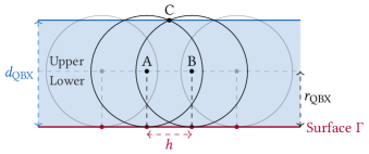
(a)

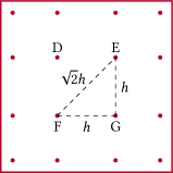
(b)

Figure 1: (a) Balls of convergence for a flat surface $\Gamma$ (c.f. Figure 7), seen from the side. (b) Grid points of $\Gamma$, seen from above. Here, $h$ is the largest spacing between grid points in each tensorial direction.

The key is to choose $d_{\text{QBX}}$ below the intersection of neighbouring balls of convergence, marked by the point C in Figure 1 (a). Since the grid on $\Gamma$ is two-dimensional, the largest distance between neighbouring grid points is not $h$ but $\sqrt{2}h$, where $h$ is as shown in Figure 1 (b). The four balls of convergence of the expansion centres above the grid points D–G in this figure intersect at distance

$$d_{\star}(h)=r_{\text{QBX}}+\sqrt{r_{\text{QBX}}^{2}-\bigg{(}\frac{\sqrt{2}h}{2}\bigg{)}^{2}}$$ (2)

from $\Gamma$. Thus, choosing $d_{\text{QBX}}\leq d_{\star}(h)$ is sufficient to ensure that all points in the upper QBX region fall within a ball of convergence. This restriction on $d_{\text{QBX}}$ can be simplified by minimizing $d_{\star}(h)$ with respect to $h$, subject to the constraint $0<h\leq r_{\text{QBX}}$. The result is

$$d_{\star\star}=\min_{0<h\leq r_{\text{QBX}}}d_{\star}(h)=d_{\star}(r_{\text{QBX}})=\left(1+\frac{1}{\sqrt{2}}\right)r_{\text{QBX}}.$$ (3)

It is thus sufficient to require that $d_{\text{QBX}}\leq d_{\star\star}$. Comparing (3) and (1), we see that the safety factor should be

$$\gamma=\frac{1}{2}\left(1+\frac{1}{\sqrt{2}}\right)\approx 0.85.$$ (4)

This derivation holds when $\Gamma$ is a flat surface, in which case the requirement (1) with $\gamma=0.85$ guarantees that all points in the upper QBX region fall within a ball of convergence, as long as $h\leq r_{\text{QBX}}$. If $\Gamma$ is curved, this guarantee holds on the concave side of $\Gamma$, but not necessarily on the convex side, where $d_{\text{QBX}}$ may have to be even smaller for the guarantee to hold. Nonetheless, we use (1) with $\gamma=0.85$ also for convex surfaces such as rods and spheroids, and it seems to work well in practice. Of course, the parameter selection strategy (section 2, step 2) will in most cases choose $d_{\text{QBX}}$ less than the upper bound $2\gamma r_{\text{QBX}}$.

Appendix D Efficient computation of streamlines in periodic flow

To compute streamlines in a periodic problem such as in section 3, we must first solve the periodic boundary integral equation as described in section 4 to get the density $\boldsymbol{q}$ on $\Gamma$. We can then compute the flow field

$$\boldsymbol{u}(\boldsymbol{x}_{\text{e}})=\boldsymbol{u}_{\text{bg}}(\boldsymbol{x}_{\text{e}})+\boldsymbol{\mathcal{D}}^{\text{3P}}[\Gamma,\boldsymbol{q}](\boldsymbol{x}_{\text{e}})+\sum_{\alpha=1}^{M}\boldsymbol{\mathcal{V}}^{(\alpha),\text{3P}}[\boldsymbol{F}^{(\alpha)},\boldsymbol{\tau}^{(\alpha)}](\boldsymbol{x}_{\text{e}})$$ (1)

at any evaluation point $\boldsymbol{x}_{\text{e}}$ in the fluid domain. To compute a streamline we pick any point $\boldsymbol{x}_{0}$ in the fluid domain and then solve the differential equation

$$\frac{\mathrm{d}\boldsymbol{x}_{\text{e}}}{\mathrm{d}t}=\boldsymbol{u}(\boldsymbol{x}_{\text{e}}(t)),\qquad\boldsymbol{x}_{\text{e}}(0)=\boldsymbol{x}_{0}.$$ (2)

Of course, (2) is discretized using some timestepping method, which must evaluate (1) at every timestep. Recall that the periodic double layer potential $\boldsymbol{\mathcal{D}}^{\text{3P}}$ is split into two parts

$$\boldsymbol{\mathcal{D}}^{\text{3P}}[\Gamma,\boldsymbol{q}](\boldsymbol{x}_{\text{e}})=\boldsymbol{\mathcal{D}}^{\text{3P,R}}[\Gamma,\boldsymbol{q}](\boldsymbol{x}_{\text{e}};\xi)+\boldsymbol{\mathcal{D}}^{\text{3P,F}}[\Gamma,\boldsymbol{q}](\boldsymbol{x}_{\text{e}};\xi)$$ (3)

and similarly for $\boldsymbol{\mathcal{V}}^{(\alpha),\text{3P}}$. The first part $\boldsymbol{\mathcal{D}}^{\text{3P,R}}$ decays fast and is treated according to section 4. The second part $\boldsymbol{\mathcal{D}}^{\text{3P,F}}$ decays slowly in real space, but since it is smooth its Fourier coefficients decay fast. In the Spectral Ewald method, $\boldsymbol{\mathcal{D}}^{\text{3P,F}}$ as given by (6) is first discretized using the direct quadrature rule (2) to give

$$\mathcal{D}_{i}^{\text{3P,F,$h$}}[\Gamma,\boldsymbol{q}](\boldsymbol{x}_{\text{e}};\xi)=\sum_{\boldsymbol{k}\in\mathbb{Z}^{3}}\sum_{s=1}^{N}T_{ijl}^{\text{F}}(\boldsymbol{x}_{\text{e}}+\boldsymbol{k}\cdot\boldsymbol{B}-\boldsymbol{x}_{s};\xi)q_{j}(\boldsymbol{x}_{s})n_{l}(\boldsymbol{x}_{s})w_{s}.$$ (4)

This is a periodic sum of point sources with strengths $Z_{jl}(\boldsymbol{x}_{s})=q_{j}(\boldsymbol{x}_{s})n_{l}(\boldsymbol{x}_{s})w_{s}$. The Spectral Ewald method [23, 31, 32] computes the periodic sum (4) in five steps:

1. Spreading point sources to a grid: A three-dimensional uniform grid is constructed over the primary cell. A window function $W(\boldsymbol{r})$ is convolved with the point sources in the primary cell to give

   $$H_{jl}(\boldsymbol{x})=\sum_{s=1}^{N}Z_{jl}(\boldsymbol{x}_{s})W([\boldsymbol{x}-\boldsymbol{x}_{s}]_{*}).$$ (5)

   Here, $[\cdot]_{*}$ denotes that the shortest periodic distance should be used, i.e.

   $$[\boldsymbol{r}]_{*}=\boldsymbol{r}+\boldsymbol{B}\cdot\operatorname*{arg\leavevmode\nobreak\ min}_{\boldsymbol{k}\in\mathbb{Z}^{3}}\lvert\boldsymbol{r}+\boldsymbol{B}\cdot\boldsymbol{k}\rvert,$$ (6)

   where $\boldsymbol{B}=(B_{1},B_{2},B_{3})$ is the size of the periodic cell. In this work the window function is a truncated Gaussian, given by $W(\boldsymbol{r})=w(r_{1})w(r_{2})w(r_{3})$, where

   $$w(r)=\begin{cases}\mathrm{e}^{-A(r/r_{\text{trunc}})^{2}},&\text{if $\lvert r\rvert\leq r_{\text{trunc}}=h_{\text{g}}P/2$},\\ 0,&\text{otherwise}.\end{cases}$$ (7)

   Here, $h_{\text{g}}$ is the grid spacing of the uniform grid, $P$ is the number of grid points within the support of $w$, and $A=0.9^{2}\pi P/2$. The parameter $P$ is chosen as discussed in [23]. It is also possible to use other window functions than the Gaussian, as discussed for example in [48].

   The function $H_{jl}(\boldsymbol{x})$ as given by (5) is evaluated on the uniform grid.

2. FFT: The three-dimensional Fourier transform $\widehat{H}_{jl}(\boldsymbol{k})$ is computed using the FFT. This is possible since $H_{jl}(\boldsymbol{x})$ is defined on a uniform grid.

3. Scaling: The result is multiplied by the Fourier transform of $\boldsymbol{T}^{\text{F}}$, and divided by the Fourier transform of the window function $W$ to undo the convolution in step 1. Since we will convolve again in step 5, this division is done twice. Thus, we here compute

   $$\widehat{\widetilde{H}}_{i}(\boldsymbol{k})=\widehat{T}^{\text{F}}_{ijl}(\boldsymbol{k};\xi)\frac{1}{[\widehat{W}(\boldsymbol{k})]^{2}}\widehat{H}_{jl}(\boldsymbol{k}),$$ (8)

   where

   $$\widehat{T}^{\text{F}}_{ijl}(\boldsymbol{k};\xi)=\sqrt{-1}\frac{\pi}{\lvert\boldsymbol{k}\rvert^{2}}\bigg{[}(\delta_{ij}k_{l}+\delta_{jl}k_{i}+\delta_{li}k_{j})-2\frac{k_{i}k_{j}k_{l}}{\lvert\boldsymbol{k}\rvert^{2}}\bigg{]}\left(8+2\frac{\lvert\boldsymbol{k}\rvert^{2}}{\xi^{2}}+\frac{\lvert\boldsymbol{k}\rvert^{4}}{\xi^{4}}\right)\mathrm{e}^{-\lvert\boldsymbol{k}\rvert^{2}/(4\xi^{2})},$$ (9)

   as given in [23].

4. IFFT: An inverse FFT is applied to $\smash{\widehat{\widetilde{H}}_{i}(\boldsymbol{k})}$ to compute $\widetilde{H}_{i}(\boldsymbol{x})$ on the uniform grid.

5. Gathering: In order to compute the final result at the evaluation point $\boldsymbol{x}_{\text{e}}$ (which need not be on the uniform grid), another convolution with the window function is performed, i.e.

   $$\mathcal{D}_{i}^{\text{3P,F,$h$}}[\Gamma,\boldsymbol{q}](\boldsymbol{x}_{\text{e}};\xi)=\int_{B}\widetilde{H}_{i}(\boldsymbol{x})W([\boldsymbol{x}_{\text{e}}-\boldsymbol{x}]_{*})\,\mathrm{d}\boldsymbol{x},$$ (10)

   where $B$ denotes the primary cell. The integral in (10) is evaluated using the trapezoidal rule on the uniform grid, which is spectrally accurate since the integrand is periodic.

Since the density $\boldsymbol{q}$ does not change during the computation of the streamlines, and the evaluation point $\boldsymbol{x}_{\text{e}}$ enters only in step 5 above, it is possible to do step 1–4 once before starting to compute the streamlines, and save $\widetilde{H}_{i}(\boldsymbol{x})$ on the uniform grid from step 4. When the Fourier-space part $\boldsymbol{\mathcal{D}}^{\text{3P,F}}[\Gamma,\boldsymbol{q}](\boldsymbol{x}_{\text{e}};\xi)$ is to be evaluated at $\boldsymbol{x}_{\text{e}}(t)$ at every timestep of solving (2), it is then enough to do only step 5. This speeds up the computation of the streamlines since evaluating (10) is fast for a single evaluation point. The real-space part $\boldsymbol{\mathcal{D}}^{\text{3P,R}}[\Gamma,\boldsymbol{q}](\boldsymbol{x}_{\text{e}};\xi)$ must be computed from scratch at every timestep, but this is fast since it is a local sum due to its rapid decay.

The periodic completion flow $\boldsymbol{\mathcal{V}}^{(\alpha),\text{3P}}$ which appears in (1) is treated in a very similar way; for details, we refer to [31, 23, 24]. Note that steps 1–5 of the Spectral Ewald method are also what is used when solving the periodic boundary integral equation as described in section 4, but in that situation all the evaluation points (i.e. the grid points of $\Gamma$) are known in advance so they can all be fed into step 5 at the same time.

References

References

- [1] K. E. Atkinson, The Numerical Solution of Integral Equations of the Second Kind, Cambridge University Press, Cambridge, 1997, doi:10.1017/CBO9780511626340.
- [2] J. Bagge, A.-K. Tornberg, Accurate quadrature methods with application to Stokes flow with particles in confined geometries, in D. J. Chappell (ed.), Proceedings of the Eleventh UK Conference on Boundary Integral Methods (UKBIM 11), Nottingham, UK, July 2017, pp. 15–24, ISBN 9780993111297. Available: http://irep.ntu.ac.uk/id/eprint/31463
- [3] A. H. Barnett, Evaluation of layer potentials close to the boundary for Laplace and Helmholtz problems on analytic planar domains, SIAM J. Sci. Comput. 36 (2), A427–A451 (2014), doi:10.1137/120900253.
- [4] A. Barnett, B. Wu, S. Veerapaneni, Spectrally accurate quadratures for evaluation of layer potentials close to the boundary for the 2D Stokes and Laplace equations, SIAM J. Sci. Comput. 37 (4), B519–B542 (2015), doi:10.1137/140990826.
- [5] J. T. Beale, M.-C. Lai, A method for computing nearly singular integrals, SIAM J. Numer. Anal. 38 (6), 1902–1925 (2001), doi:10.1137/S0036142999362845.
- [6] J. T. Beale, W. Ying, J. R. Wilson, A Simple Method for Computing Singular or Nearly Singular Integrals on Closed Surfaces, Commun. Comput. Phys. 20 (3), 733–753 (2016), doi:10.4208/cicp.030815.240216a.
- [7] J.-P. Berrut, L. N. Trefethen, Barycentric Lagrange Interpolation, SIAM Rev. 46 (3), 501–517 (2004), doi:10.1137/S0036144502417715.
- [8] J. R. Blake, A note on the image system for a stokeslet in a no-slip boundary, Proc. Camb. Phil. Soc. 70 (2), 303–310 (1971), doi:10.1017/S0305004100049902.
- [9] O. P. Bruno, L. A. Kunyansky, A Fast, High-Order Algorithm for the Solution of Surface Scattering Problems: Basic Implementation, Tests, and Applications, J. Comp. Phys. 169 (1), 80–110 (2001), doi:10.1006/jcph.2001.6714.
- [10] C. Carvalho, S. Khatri, A. D. Kim, Close evaluation of layer potentials in three dimensions, arXiv:1807.02474 [math.NA] (2018).
- [11] C. Carvalho, S. Khatri, A. D. Kim, Asymptotic approximations for the close evaluation of double-layer potentials, arXiv:1810.02483 [math.NA] (2018).
- [12] E. Corona, S. Veerapaneni, Boundary integral equation analysis for suspension of spheres in Stokes flow, J. Comp. Phys. 362, 327–345 (2018), doi:10.1016/j.jcp.2018.02.017.
- [13] M. Deserno, C. Holm, How to mesh up Ewald sums. I. A theoretical and numerical comparison of various particle mesh routines, J. Chem. Phys. 109 (18), 7678–7693 (1998), doi:10.1063/1.477414.
- [14] C. L. Epstein, L. Greengard, A. Klöckner, On the convergence of local expansions of layer potentials, SIAM J. Numer. Anal. 51 (5), 2660–2679 (2013), doi:10.1137/120902859.
- [15] Z. Gimbutas, L. Greengard, S. Veerapaneni, Simple and efficient representations for the fundamental solutions of Stokes flow in a half-space, J. Fluid Mech. 776, R1 (2015), doi:10.1017/jfm.2015.302.
- [16] R. G. Gontijo, F. R. Cunha, Dynamic numerical simulations of magnetically interacting suspensions in creeping flow, Powder Technol. 279, 146–165 (2015), doi:10.1016/j.powtec.2015.03.033.
- [17] L. Greengard, V. Rokhlin, A fast algorithm for particle simulations, J. Comp. Phys. 73 (2), 325–348 (1987), doi:10.1016/0021-9991(87)90140-9.
- [18] L. Greengard, V. Rokhlin, A new version of the Fast Multipole Method for the Laplace equation in three dimensions, Acta Numer. 6, 229–269 (1997), doi:10.1017/S0962492900002725.
- [19] J. S. Guasto, A. S. Ross, J. P. Gollub, Hydrodynamic irreversibility in particle suspensions with nonuniform strain, Phys. Rev. E 81 (6), 061401 (2010), doi:10.1103/PhysRevE.81.061401.
- [20] J. S. Guasto, R. Rusconi, R. Stocker, Fluid Mechanics of Planktonic Microorganisms, Annu. Rev. Fluid Mech. 44, 373–400 (2012), doi:10.1146/annurev-fluid-120710-101156.
- [21] J. Helsing, R. Ojala, On the evaluation of layer potentials close to their sources, J. Comp. Phys. 227 (5), 2899–2921 (2008), doi:10.1016/j.jcp.2007.11.024.
- [22] S. Kim, S. J. Karrila, Microhydrodynamics : Principles and Selected Applications, Butterworth–Heinemann, Boston, 1991, doi:10.1016/C2013-0-04644-0.
- [23] L. af Klinteberg, A.-K. Tornberg, Fast Ewald summation for Stokesian particle suspensions, Int. J. Numer. Methods Fluids 76 (10), 669–698 (2014), doi:10.1002/fld.3953.
- [24] L. af Klinteberg, Ewald summation for the rotlet singularity of Stokes flow, arXiv:1603.07467 [physics.flu-dyn] (2016).
- [25] L. af Klinteberg, A.-K. Tornberg, A fast integral equation method for solid particles in viscous flow using quadrature by expansion, J. Comp. Phys. 326, 420–445 (2016), doi:10.1016/j.jcp.2016.09.006.
- [26] L. af Klinteberg, A.-K. Tornberg, Error estimation for quadrature by expansion in layer potential evaluation, Adv. Comput. Math. 43, 195–234 (2017), doi:10.1007/s10444-016-9484-x.
- [27] L. af Klinteberg, D. Saffar Shamshirgar, A.-K. Tornberg, Fast Ewald summation for free-space Stokes potentials, Res. Math. Sci. 4 (1), (2017), doi:10.1186/s40687-016-0092-7.
- [28] L. af Klinteberg, A.-K. Tornberg, Adaptive quadrature by expansion for layer potential evaluation in two dimensions, SIAM J. Sci. Comput. 40 (3), A1225–A1249 (2018), doi:10.1137/17M1121615.
- [29] A. Klöckner, A. Barnett, L. Greengard, M. O’Neil, Quadrature by expansion: A new method for the evaluation of layer potentials, J. Comp. Phys. 252, 332–349 (2013), doi:10.1016/j.jcp.2013.06.027.
- [30] R. Kress, Linear Integral Equations, Springer, New York, 3rd ed., 2014, doi:10.1007/978-1-4614-9593-2.
- [31] D. Lindbo, A.-K. Tornberg, Spectrally accurate fast summation for periodic Stokes potentials, J. Comp. Phys. 229 (23), 8994–9010 (2010), doi:10.1016/j.jcp.2010.08.026.
- [32] D. Lindbo, A.-K. Tornberg, Spectral accuracy in fast Ewald-based methods for particle simulations, J. Comp. Phys. 230 (24), 8744–8761 (2011), doi:10.1016/j.jcp.2011.08.022.
- [33] D. Lindbo, L. af Klinteberg, D. Saffar Shamshirgar, The spectral Ewald unified package, http://github.com/ludvigak/SE_unified, 2018.
- [34] L. Lu, M. J. Morse, A. Rahimian, G. Stadler, D. Zorin, Scalable Simulation of Realistic Volume Fraction Red Blood Cell Flows through Vascular Networks, in Proceedings of the International Conference for High Performance Computing, Networking, Storage and Analysis (SC ’19), Denver, CO, USA, November 2019, article 6, doi:10.1145/3295500.3356203.
- [35] D. Malhotra, A. Rahimian, D. Zorin, G. Biros, A parallel algorithm for long-timescale simulation of concentrated vesicle suspensions in three dimensions, 2018. Preprint available: https://cims.nyu.edu/~malhotra/files/pubs/ves3d.pdf
- [36] N. Mittal, F. Ansari, K. Gowda. V, C. Brouzet, P. Chen, P. T. Larsson, S. V. Roth, F. Lundell, L. Wågberg, N. A. Kotov, L. D. Söderberg, Multiscale Control of Nanocellulose Assembly: Transferring Remarkable Nanoscale Fibril Mechanics to Macroscale Fibers, ACS Nano 12 (7), 6378–6388 (2018), doi:10.1021/acsnano.8b01084.
- [37] R. Ojala, A.-K. Tornberg, An accurate integral equation method for simulating multi-phase Stokes flow, J. Comp. Phys. 298, 145–160 (2015), doi:10.1016/j.jcp.2015.06.002.
- [38] F. W. J. Olver, A. B. Olde Daalhuis, D. W. Lozier, B. I. Schneider, R. F. Boisvert, C. W. Clark, B. R. Miller, B. V. Saunders, H. S. Cohl, M. A. McClain, NIST Digital Library of Mathematical Functions, http://dlmf.nist.gov/, Release 1.0.25 of 2019-12-15.
- [39] S. Pålsson, M. Siegel, A.-K. Tornberg, Simulation and validation of surfactant-laden drops in two-dimensional Stokes flow, J. Comp. Phys. 386, 218–247 (2019), doi:10.1016/j.jcp.2018.12.044.
- [40] C. Pérez-Arancibia, L. M. Faria, C. Turc, Harmonic density interpolation methods for high-order evaluation of Laplace layer potentials in 2D and 3D, J. Comp. Phys. 376, 411–434 (2019), doi:10.1016/j.jcp.2018.10.002.
- [41] H. Power, G. Miranda, Second kind integral equation formulation of Stokes’ flows past a particle of arbitrary shape, SIAM J. Appl. Math. 47 (4), 689–698 (1987), doi:10.1137/0147047.
- [42] C. Pozrikidis, Boundary integral and singularity methods for linearized viscous flow, Cambridge University Press, Cambridge, 1992, doi:10.1017/CBO9780511624124.
- [43] M. Rachh, Integral equation methods for problems in electrostatics, elastostatics and viscous flow, PhD Thesis, New York University, 2015, ISBN 978-1-321-95485-2. Available: https://search.proquest.com/docview/1710781501
- [44] M. Rachh, A. Klöckner, M. O’Neil, Fast algorithms for Quadrature by Expansion I: Globally valid expansions, J. Comp. Phys. 345, 706–731 (2017), doi:10.1016/j.jcp.2017.04.062.
- [45] A. Rahimian, A. Barnett, D. Zorin, Ubiquitous evaluation of layer potentials using Quadrature by Kernel-Independent Expansion, BIT Numer. Math. 58, 423–456 (2018), doi:10.1007/s10543-017-0689-2.
- [46] S. Reddig, H. Stark, Nonlinear dynamics of spherical particles in Poiseuille flow under creeping-flow condition, J. Chem. Phys. 138 (23), 234902 (2013), doi:10.1063/1.4809989.
- [47] Y. Saad, M. H. Schultz, GMRES: A generalized minimal residual algorithm for solving nonsymmetric linear systems, SIAM J. Sci. Stat. Comput. 7 (3), 856–869 (1986), doi:10.1137/0907058.
- [48] D. Saffar Shamshirgar, A.-K. Tornberg, Fast Ewald summation for electrostatic potentials with arbitrary periodicity, arXiv:1712.04732 [math.NA] (2017).
- [49] M. Siegel, A.-K. Tornberg, A local target specific quadrature by expansion method for evaluation of layer potentials in 3D, J. Comp. Phys. 364, 365–392 (2018), doi:10.1016/j.jcp.2018.03.006.
- [50] C. Sorgentone, A.-K. Tornberg, A highly accurate boundary integral equation method for surfactant-laden drops in 3D, J. Comp. Phys. 360, 167–191 (2018), doi:10.1016/j.jcp.2018.01.033.
- [51] T. M. Squires, S. R. Quake, Microfluidics: Fluid physics at the nanoliter scale, Rev. Mod. Phys. 77 (3), 977–1026 (2005), doi:10.1103/RevModPhys.77.977.
- [52] S. Srinivasan, A.-K. Tornberg, Fast Ewald summation for Green’s functions of Stokes flow in a half-space, Res. Math. Sci. 5 (3), article 35 (2018), doi:10.1007/s40687-018-0153-1.
- [53] S. Tlupova, J. T. Beale, Nearly Singular Integrals in 3D Stokes Flow, Commun. Comput. Phys. 14 (5), 1207–1227 (2013), doi:10.4208/cicp.020812.080213a.
- [54] S. Tlupova, J. T. Beale, Regularized single and double layer integrals in 3D Stokes flow, J. Comp. Phys. 386, 568–584 (2019), doi:10.1016/j.jcp.2019.02.031.
- [55] A.-K. Tornberg, L. Greengard, A fast multipole method for the three-dimensional Stokes equations, J. Comp. Phys. 227 (3), 1613–1619 (2008), doi:10.1016/j.jcp.2007.06.029.
- [56] L. N. Trefethen, J. A. C. Weideman, The Exponentially Convergent Trapezoidal Rule, SIAM Rev. 56 (3), 385–458 (2014), doi:10.1137/130932132.
- [57] L. Ying, G. Biros, D. Zorin, A high-order 3D boundary integral equation solver for elliptic PDEs in smooth domains, J. Comp. Phys. 219, 247–275 (2006), doi:10.1016/j.jcp.2006.03.021.
- [58] M. Wala, A. Klöckner, A fast algorithm with error bounds for Quadrature by Expansion, J. Comp. Phys. 374, 135–162 (2018), doi:10.1016/j.jcp.2018.05.006.
- [59] M. Wala, A. Klöckner, A fast algorithm for Quadrature by Expansion in three dimensions, J. Comp. Phys. 388, 655–689 (2019), doi:10.1016/j.jcp.2019.03.024.
- [60] M. Wala, A. Klöckner, Optimization of fast algorithms for global Quadrature by Expansion using target-specific expansions, J. Comp. Phys. 403, 108976 (2020), doi:10.1016/j.jcp.2019.108976.
- [61] H. Zhao, A. H. G. Isfahani, L. N. Olson, J. B. Freund, A spectral boundary integral method for flowing blood cells, J. Comp. Phys. 229, 3726–3744 (2010), doi:10.1016/j.jcp.2010.01.024.