Systematic construction of square-root topological insulators and superconductors

Abstract

We propose a general scheme to construct a Hamiltonian $H_{\text{root}}$ describing a square root of an original Hamiltonian $H_{\text{original}}$ based on the graph theory. The square-root Hamiltonian is defined on the subdivided graph of the original graph of $H_{\text{original}}$, where the subdivided graph is obtained by putting one vertex on each link in the original graph. When $H_{\text{original}}$ describes a topological system, there emerge in-gap edge states at non-zero energy in the spectrum of $H_{\text{root}}$, which are the inherence of the topological edge states at zero energy in $H_{\text{original}}$. In this case, $H_{\text{root}}$ describes a square-root topological insulator or superconductor. Typical examples are square roots of the Su-Schrieffer-Heeger (SSH) model, the Kitaev topological superconductor model and the Haldane model. Our scheme is also applicable to non-Hermitian topological systems, where we study an example of a nonreciprocal non-Hermitian SSH model.

Introduction: Topological insulators and superconductors are among the most studied fields in condensed matter physics in this decadeHasan ; Qi . They are characterized by the bulk-edge correspondence, i.e., by the emergence of topological edge states although the bulk is gapped.

Recently, a square-root topological insulator is proposedArk ; Kremer . Its notion has also been generalized to square-root higher-order topological insulatorsHatsugai . They are characterized by the emergence of in-gap edge states at nonzero energy, which are the inherence of the topological edge states at zero energy of the original HamiltonianArk ; Kremer .

In this paper, we propose a general scheme to construct square-root topological insulators and superconductors from ordinary topological insulators and superconductors based on the graph theory. There is one-to-one correspondence between a tight-binding Hamiltonian and a weighted graph. A graph is composed of vertices and links. We can construct a new graph by introducing one vertex on each link, which we refer to as the subdivided graphEzawaSch ; EzawaUniv . We call the original graph the parent graph in contrast to the subdivided graph. Any subdivided graph is bipartite because it contains original vertices and newly added vertices. Examples are shown in Figs.1, 2 and 3, where original (new) vertices are shown in magenta (cyan).

We denote the Hamiltonian constructed on the subdivided graph as $H_{\text{root}}$. We then find $(H_{\text{root}})^{2}=H_{\text{par}}\oplus H_{\text{res}}$, where $H_{\text{par}}$ is identical to the original Hamiltonian $H_{\text{original}}$ up to an additive constant interpreted as a self-energy. We call $H_{\text{par}}$ and $H_{\text{res}}$ the parent and residual Hamiltonians, respectively. When $H_{\text{original}}$ describes a topological system, it contains zero-energy topological boundary states, producing the corresponding boundary states at nonzero energy in $H_{\text{root}}$. Furthermore, zero-energy perfect-flat bulk-bands may emerge in $H_{\text{root}}$ as a bipartite property according to the Lieb theorem: See orange lines in Figs.2 and 3. Because the eigenvalues are shown to be identical between $H_{\text{par}}$ and $H_{\text{res}}$ except for zero-energy states in $H_{\text{res}}$, $H_{\text{root}}$ is interpreted as the square-root Hamiltonian of $H_{\text{original}}$. We can use the same topological index between $H_{\text{root}}$ and $H_{\text{original}}$ since the eigenvectors are identical between them. Indeed, the region of the in-gap edge states in $H_{\text{root}}$ is precisely the same as that of the zero-energy edge states in $H_{\text{original}}$.

We present explicit examples of the Su-Schrieffer-Heeger (SSH), the Kitaev $p$-wave topological superconductor model and the Haldane honeycomb model. Furthermore, our results are applicable to non-Hermitian systems, where we demonstrate an example of nonreciprocal non-Hermitian SSH model.

Square-root Hamiltonian: It is impossible to construct a local hopping model only by taking a square root of the Hamiltonian matrix. A simple example is given by the SSH model,

$$H_{\text{SSH}}=\left(\begin{array}[]{cc}0&t_{a}+t_{b}e^{-ik}\\ t_{a}+t_{b}e^{ik}&0\end{array}\right).$$ (1)

A square root of the model is given byNoteSM1

$$\sqrt{H_{\text{SSH}}}=\left(\begin{array}[]{cc}0&\frac{\sqrt{E\left(k\right)}}{t_{a}+t_{b}e^{-ik}}\\ \frac{t_{a}+t_{b}e^{-ik}}{\sqrt{E\left(k\right)}}&0\end{array}\right),$$ (2)

with $E\left(k\right)=\sqrt{t_{a}^{2}+t_{b}^{2}+2t_{a}t_{b}\cos k}$. This is an infinite-range hopping model.

Here we recall the Dirac idea to take a square root of the Klein-Gordon equation. He obtained the Dirac equation by introducing a matrix degree of freedom. The Dirac equation has various intriguing properties such as chirality and the index theorem, which are absent in the Klein-Gordon equation.

We propose to take a square root of a Hamiltonian by increasing a matrix degree of freedom as follows: 1) We first write down a graph representation of the adjacency matrix of the original Hamiltonian $H_{\text{original}}$. 2) We construct a subdivided graph from the original graph. 3) We construct a Hamiltonian $H_{\text{root}}$ on the subdivided graph. Then, we obtain $(H_{\text{root}})^{2}=H_{\text{par}}\oplus H_{\text{res}}$, where $H_{\text{par}}$ is identical to the original Hamiltonian $H_{\text{original}}$ up to an additive constant, provided the hopping parameter is taken to be $\sqrt{t}$ in $H_{\text{root}}$ corresponding to the hopping parameter $t$ in $H_{\text{original}}$. The square-root Hamiltonian is given by $H_{\text{root}}$.

We start with a Hamiltonian $H_{\text{original}}$ where a unit cell contains $N$ sites connected by $M$ hoppings. We consider a Hamiltonian on the subdivided graph, which is given by

$$H_{\text{root}}=\left(\begin{array}[]{cc}O_{N\times N}&H_{N\times M}^{\text{left}}\\ H_{M\times N}^{\text{right}}&O_{M\times M}\end{array}\right).$$ (3)

It is required that $H_{M\times N}^{\text{right}}=(H_{N\times M}^{\text{left}})^{\dagger}$, when $H_{\text{root}}$ is Hermitian. We have

$$(H_{\text{root}})^{2}=\left(\begin{array}[]{cc}H_{\text{par}}&0\\ 0&H_{\text{res}}\end{array}\right)=H_{\text{par}}\oplus H_{\text{res}},$$ (4)

where

$$H_{\text{par}}\equiv H_{N\times M}^{\text{left}}H_{M\times N}^{\text{right}},\quad H_{\text{res}}\equiv H_{M\times N}^{\text{right}}H_{N\times M}^{\text{left}}.$$ (5)

Thus the square of the Hamiltonian, $(H_{\text{root}})^{2}$, is decomposed into a direct sum of $H_{\text{par}}$ and $H_{\text{res}}$, which are the parent and residual Hamiltonians defined on the parent and residual graphs.

In general, $H_{\text{par}}$ is identical to $H_{\text{original}}$ up to a constant term because both of them are constructed on the same graph,

$$H_{\text{par}}=C+H_{\text{original}},$$ (6)

where $C$ is a positive constant obtained by calculating $(H_{\text{root}})^{2}$. This constant term can be interpreted as a self energy, as in the case of the second-order perturbation theory. The zero-energy topological edge states in $H_{\text{original}}$ are transformed into the in-gap boundary states at non-zero energy $\pm\sqrt{C}$ in $H_{\text{root}}$.

The bipartite Hamiltonian has chiral symmetry, $\{\gamma,H_{\text{root}}\}=0$, with the chiral operator defined by

$$\gamma=\left(\begin{array}[]{cc}I_{N\times N}&O_{N\times M}\\ O_{M\times N}&-I_{M\times M}\end{array}\right).$$ (7)

In general, we have $M>N$. According to the Lieb theoremLieb , there are $\left|M-N\right|$ zero-energy states constituting perfect-flat bulk bands.

It is knownDas ; Tsune ; NoteSM2 that the eigenvalues are identical between $H_{\text{par}}$ and $H_{\text{res}}$ except for these zero-energy states in $H_{\text{res}}$ and that they are non-negative. Namely, when we set

$$H_{\text{par}}|\psi_{j}^{\text{par}}\rangle=\varepsilon_{j}|\psi_{j}^{\text{par}}\rangle,\quad H_{\text{res}}|\psi_{j}^{\text{res}}\rangle=\varepsilon_{j}^{\text{res}}|\psi_{j}^{\text{res}}\rangle,$$ (8)

we obtain $\{\varepsilon_{j}^{\text{res}}\}=\{\varepsilon_{1},\cdots\varepsilon_{N},0,\cdots,0\}$ and $\varepsilon_{j}\geq 0$. It follows from (6) that the eigenvectors of $H_{\text{par}}$ and $H_{\text{original}}$ are the same, $H_{\text{original}}|\psi_{j}^{\text{par}}\rangle=(\varepsilon_{j}-C)|\psi_{j}^{\text{par}}\rangle$. Furthermore, the eigenvectors $|\psi_{j}^{\text{res}}\rangle$ of $H_{\text{res}}$ are obtained from those of $H_{\text{par}}$ asNoteSM2

$$|\psi_{j}^{\text{res}}\rangle\equiv\sum_{k}(H_{M\times N}^{\text{right}})_{jk}|\psi_{k}^{\text{par}}\rangle.$$ (9)

The eigenvectors of $(H_{\text{root}})^{2}$ are given by

$$|\psi_{j}^{\text{root}}\rangle=\{\psi_{1}^{\text{par}},\cdots,\psi_{N}^{\text{par}},\psi_{1}^{\text{res}},\cdots,\psi_{M}^{\text{res}}\}.$$ (10)

When the Hamiltonian $H_{\text{root}}$ is diagonalized by a unitary transformation $U$ as $U^{\dagger}H_{\text{root}}U=H_{\text{root}}^{\text{D}}$, the Hamiltonian $(H_{\text{root}})^{2}$ is also diagonalized by the same unitary transformation as $U^{\dagger}(H_{\text{root}})^{2}U=(H_{\text{root}}^{\text{D}})^{2}$. Then, the eigenvalues of $H_{\text{root}}$ are obtained just by taking a square root of them with the same eigenvectors,

$$H_{\text{root}}|\psi_{j}^{\text{root}}\rangle=\varepsilon_{j}^{\text{root}}|\psi_{j}^{\text{root}}\rangle,$$ (11)

where

$$\varepsilon_{j}^{\text{root}}=\{\pm\sqrt{\varepsilon_{1}},\cdots,\pm\sqrt{\varepsilon_{N}};\pm\sqrt{\varepsilon_{1}},\cdots,\pm\sqrt{\varepsilon_{N}},0,\cdots,0\}.$$ (12)

Because of this property, $H_{\text{root}}$ is interpreted as the square-root Hamiltonian of $H_{\text{original}}$.

An important observation is that the topolgocal properties are identical between $H_{\text{root}}$ and $H_{\text{original}}$ since the eigenvectors are the same. Correspondingly, the topological indices are the same.

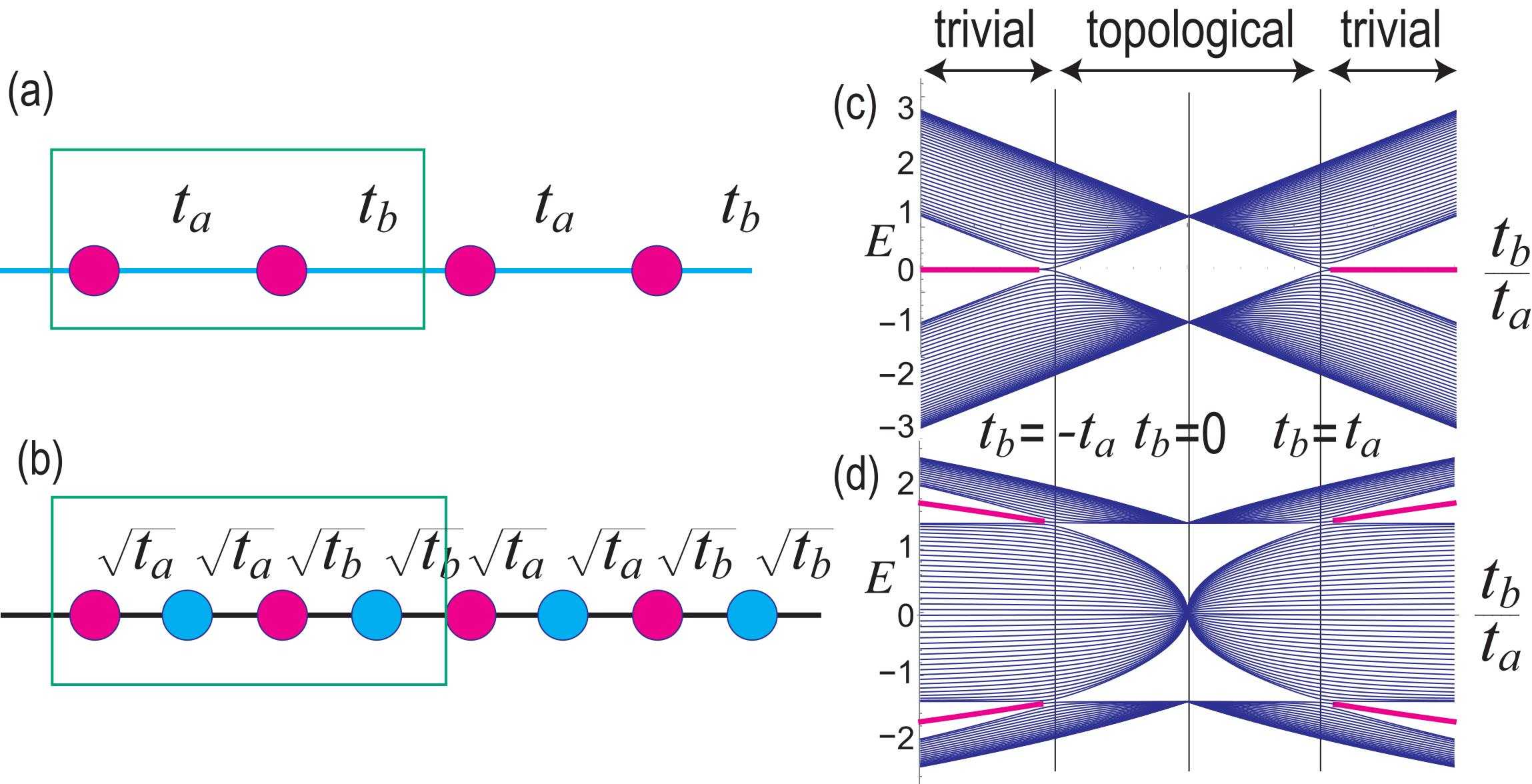
Figure 1: Illustration of (a) the graph and (b) the subdivided graph for the SSH model $H_{\text{SSH}}$. The green rectangles represent the unit cells. (c) Energy spectrum of $H_{\text{SSH}}$ and (d) $H_{\text{root}}$ in unit of $t_{a}$ as a function of $t_{b}/t_{a}$. The topological edge states are marked in magenta. In-gap edge states are on the curve $E=\pm\sqrt{\left|t_{a}\right|+\left|t_{b}\right|}$ for $H_{\text{root}}$.

Square-root SSH model: For the first example, we analyze the SSH model (1). The spectrum contains the zero-energy topological edge states as in Fig.1(c). The graph of the SSH model is a simple one-dimensional graph containing two vertices in the unit cell [Fig.1(a)]. The corresponding subdivided graph is a one-dimensional graph containing four vertices in the unit cell [Fig.1(b)]. The square-root Hamiltonian $H_{\text{root}}$ is given by (3) with $(N,M)=(2,2)$, and

$$H_{2\times 2}^{\text{left}}=\left(\begin{array}[]{cc}\sqrt{t_{a}}&\sqrt{t_{b}}e^{-ik}\\ \sqrt{t_{a}}&\sqrt{t_{b}}\end{array}\right).$$ (13)

It is straightforward to derive $(H_{\text{root}})^{2}=H_{\text{par}}\oplus H_{\text{res}}$ with

$$H_{\text{par}} =\left|t_{a}\right|+\left|t_{b}\right|+H_{\text{SSH}},$$ (14)

$$H_{\text{res}} =\left(\begin{array}[]{cc}2t_{a}&\sqrt{t_{a}t_{b}}\left(1+e^{-ik}\right)\\ \sqrt{t_{a}t_{b}}\left(1+e^{ik}\right)&2t_{b}\end{array}\right),$$ (17)

where $H_{\text{res}}$ is the Rice-Mele model. In-gap edge states appear at $E=\pm\sqrt{\left|t_{a}\right|+\left|t_{b}\right|}$ for $\left|t_{b}\right|>\left|t_{a}\right|$, as illustrated in Fig.1(d), whose origin is the topological zero-energy states in the SSH model [Fig.1(c)].

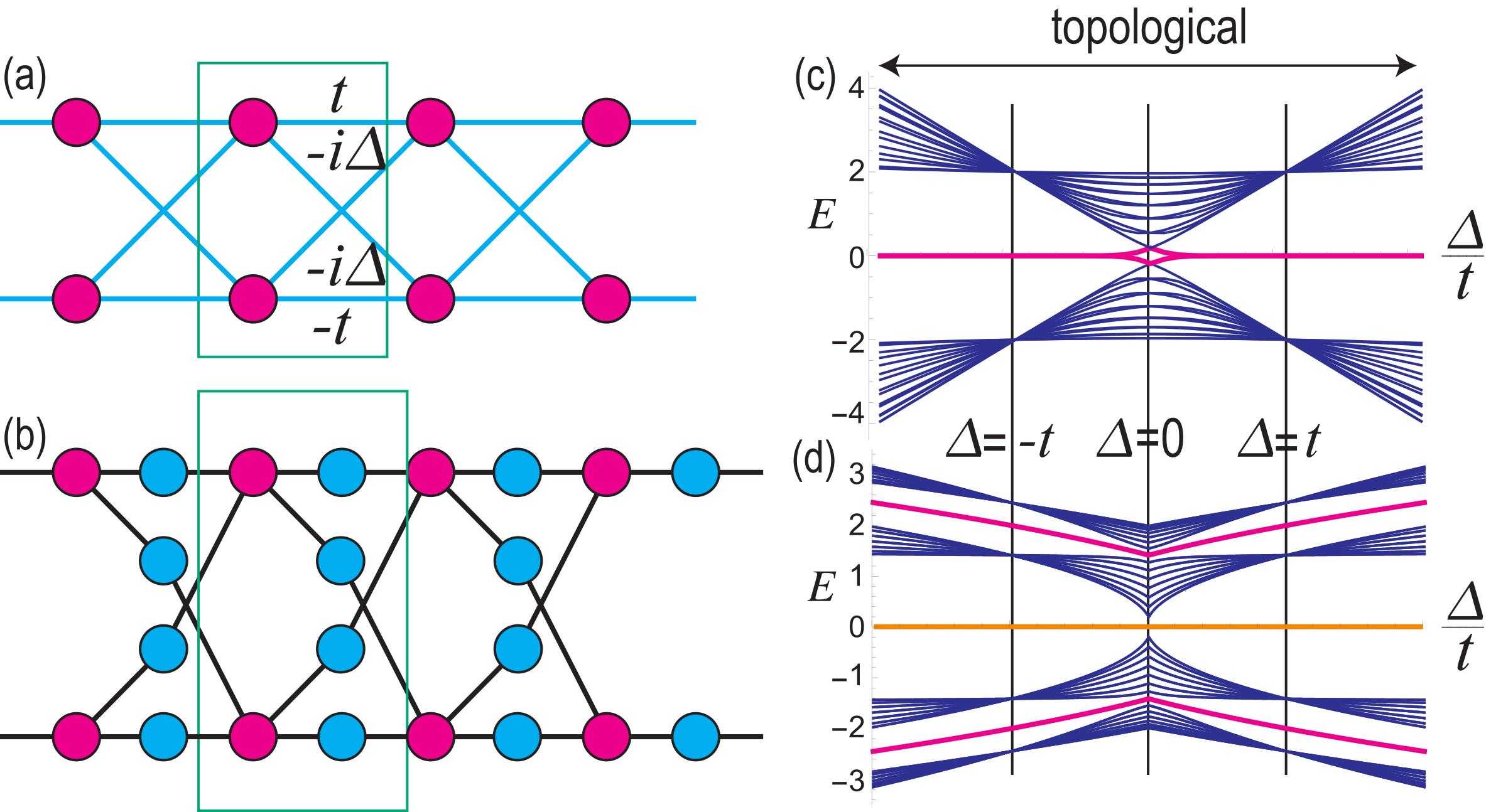
Figure 2: Illustration of (a) the graph and (b) the subdivided graph for the Kitaev model $H_{\text{Kitaev}}$. (c) Energy spectrum of $H_{\text{Kitaev}}$ and (d) $H_{\text{root}}$ in unit of $t$ as a function of $\Delta/t$. The topological edge states are marked in magenta. In-gap states are on the curve $E=\pm\sqrt{2\left|t\right|+2\left|\Delta\right|}$ for $H_{\text{root}}$. Lieb perfect-flat bulk-bands are marked in orange.

Square-root Kitaev topological superconductor: The next example is a square root of the Kitaev $p$-wave topological superconductor model defined byKitaev ; Alicea ; Flen ; Beenakker

$$H_{\text{Kitaev}}=\left(2t\cos k-\mu\right)\sigma_{z}+2\Delta\sigma_{x}\sin k.$$ (18)

The spectrum contains the zero-energy topological edge states as in Fig.2(c). The corresponding graph and subdivided graph are shown in Fig.2(a) and (b). The square-root Hamiltonian $H_{\text{root}}$ is given the Hamiltonian (3) with $(N,M)=(2,4)$, and

$$H_{2\times 4}^{\text{left}}=\left(\begin{array}[]{cccc}\sqrt{t}\left(1+e^{-ik}\right)&0&\Delta^{\prime}&\Delta^{\prime\ast}e^{-ik}\\ 0&i\sqrt{t}\left(1-e^{-ik}\right)&\Delta^{\prime\ast}e^{-ik}&\Delta^{\prime}\end{array}\right),$$ (19)

where $\Delta^{\prime}=e^{-i\pi/4}\sqrt{\Delta}$.

We calculate $(H_{\text{root}})^{2}=H_{\text{par}}\oplus H_{\text{res}}$. The parent Hamiltonian $H_{\text{par}}$ is found to be the Kitaev HamiltonianKitaev ; Alicea ; Flen ; Beenakker with $\mu=0$ and the addition of a constant term $2\left|t\right|+2\left|\Delta\right|$. In-gap edge states appear in $H_{\text{root}}$ at $E=\pm\sqrt{2\left|t\right|+2\left|\Delta\right|}$ as in Fig.2(d), which are transformed from the zero-energy topological states in the Kitaev model[Fig.2(c)]. Furthermore, there are perfect-flat bulk-bands at zero energy in $H_{\text{root}}$ due to the Lieb theoremLieb with $\left|M-N\right|=2$.

Square-root Haldane model: We next study a square root of the Haldane model. The Hamiltonian is defined on the graph in Fig.3(a) and given by

$$H_{\text{Haldane}} =2\lambda\left(2\sin\frac{k_{x}}{2}\cos\frac{\sqrt{3}k_{y}}{2}-\sin k_{x}\right)\sigma_{z}$$

$$+t\left(1+\cos\frac{\sqrt{3}k_{x}}{2}\cos\frac{k_{y}}{2}\right)\sigma_{x}$$

$$+t\left(\cos\frac{\sqrt{3}k_{x}}{2}\sin\frac{k_{y}}{2}\right)\sigma_{y}.$$ (20)

The spectrum in nanoribbon geometry contains chiral edge states as in Fig.3(c). The subdivided graph of the honeycomb graph is shown in Fig.3(b). The square-root Hamiltonian $H_{\text{root}}$ is given by the Hamiltonian (3) with $(N,M)=(2,9)$ and $H_{2\times 9}=\{a_{ij}\}$, where $a_{11}=\sqrt{t}$, $a_{12}=\sqrt{t}e^{i\boldsymbol{k}\cdot\boldsymbol{a}_{2}}$, $a_{13}=\sqrt{t}e^{-i\boldsymbol{k}\cdot\boldsymbol{a}_{1}}$, $a_{14}=\lambda+\lambda^{\ast}e^{i\boldsymbol{k}\cdot\boldsymbol{a}_{2}}$, $a_{15}=\lambda^{\ast}+\lambda e^{-i\boldsymbol{k}\cdot\boldsymbol{a}_{1}}$, $a_{16}=a_{17}=a_{18}=0$, $a_{19}=\lambda+\lambda^{\ast}e^{-ik_{x}}$, $a_{21}=a_{22}=a_{23}=\sqrt{t}$, $a_{24}=a_{25}=0$, $a_{26}=\lambda^{\ast}+\lambda e^{i\boldsymbol{k}\cdot\boldsymbol{a}_{1}}$, $a_{27}=\lambda+\lambda^{\ast}e^{-i\boldsymbol{k}\cdot\boldsymbol{a}_{2}}$, $a_{28}=\lambda^{\ast}+\lambda e^{-ik_{x}}$, $a_{29}=0$ and $\boldsymbol{a}_{1}=\left\{\sqrt{3}/2,1/2\right\}$, $\boldsymbol{a}_{2}=\left\{\sqrt{3}/2,-1/2\right\}$. The parent Hamiltonian $H_{\text{par}}$ is found to be

$$H_{\text{par}}=3\left(\left|t\right|+2\left|\lambda\right|\right)+H_{\text{Haldane}}.$$ (21)

The chiral edge state in nanoribbon geometry emerges in $H_{\text{root}}$, as shown in Fig.3(d). Furthermore, there are $7$ zero energy states in $H_{\text{total}}$ due to the Lieb theoremLieb with $\left|M-N\right|=7$.

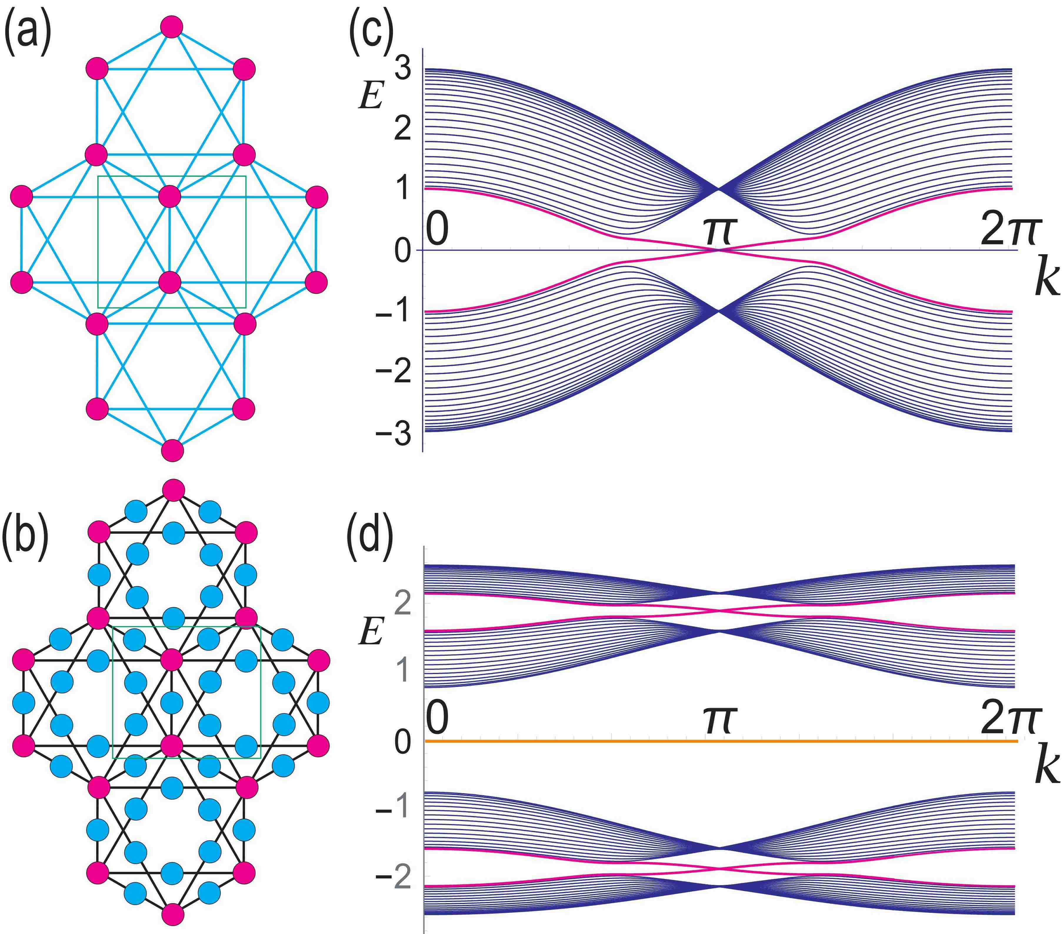
Figure 3: Illustration of (a) the graph and (b) the subdivided graph for the Haldane model $H_{\text{Haldane}}$. (c) Energy spectrum of $H_{\text{Haldane}}$ and (d) $H_{\text{root}}$ in unit of $t$ as a function of the momentum $k$. The chiral edge states are marked in magenta. Lieb perfect-flat bulk-bands are marked in orange. We have set $\lambda=0.2t/(3\sqrt{3})$.

Square-root non-Hermitian SSH model: We proceed to construct a square root of a non-Hermitian SSH model by introducing the nonreciprocity $\gamma$, as illustrated in Fig.4(a). The Hamiltonian readsScho ; Lieu ; Lee ; Yin ; Yao ; EzawaSSH

$$H_{\text{SSH}}^{\text{non}}=\left(\begin{array}[]{cc}0&t_{a}+\left(t_{b}+\gamma\right)e^{-ik}\\ t_{a}+\left(t_{b}-\gamma\right)e^{ik}&0\end{array}\right),$$ (22)

where the hopping amplitudes are different between left and right goings. The spectrum contains zero-energy edges states in the topological phase, whose real and imaginary parts are shown in Fig.4(c) and (c’). The square-root Hamiltonian $H_{\text{root}}$ is defined on the subdivided graph in Fig.4(b), and given by the Hamiltonian (3) with

$$H_{2\times 2}^{\text{left}} =\left(\begin{array}[]{cc}t_{a}&\sqrt{t_{b}+\gamma}e^{-ik}\\ t_{a}&\sqrt{t_{b}-\gamma}\end{array}\right),$$ (25)

$$H_{2\times 2}^{\text{right}} =\left(\begin{array}[]{cc}t_{a}&t_{a}\\ \sqrt{t_{b}-\gamma}e^{ik}&\sqrt{t_{b}+\gamma}\end{array}\right).$$ (28)

The parent Hamiltonian $H_{\text{par}}$ is found to be

$$H_{\text{par}}=\left|t_{a}\right|+\sqrt{t_{b}^{2}-\gamma^{2}}+H_{\text{SSH}}^{\text{non}}.$$ (29)

The residual Hamiltonian is given by $H_{\text{res}}=\{a_{ij}\}$, where $a_{11}=2t_{a}$, $a_{12}=\sqrt{t_{a}}\left(\sqrt{t_{b}-\gamma}+\sqrt{t_{b}+\gamma}e^{ik}\right)$, $a_{21}=\sqrt{t_{a}}\left(\sqrt{t_{b}+\gamma}+\sqrt{t_{b}-\gamma}e^{ik}\right)$, $a_{22}=2\sqrt{t_{b}^{2}-\gamma^{2}}$. In-gap edge states emerge at $E=\pm\sqrt{\left|t_{a}\right|+\sqrt{t_{b}^{2}-\gamma^{2}}}$ for $\left|t_{a}\right|>\left|t_{b}\right|$ in $H_{\text{root}}$, as shown in Fig.4(d), which are transformed from the zero-energy topological edge states in $H_{\text{SSH}}^{\text{non}}$.

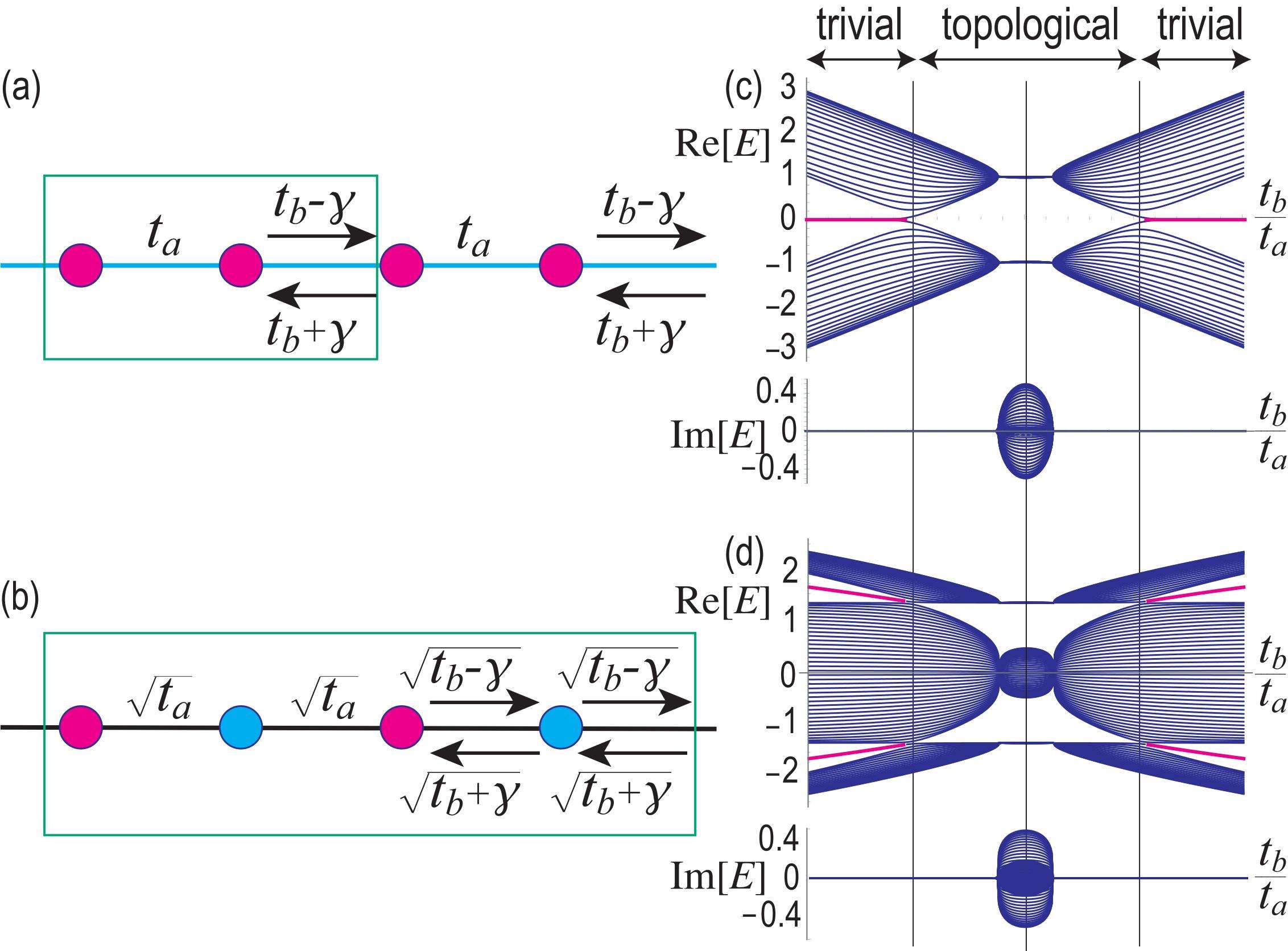
Figure 4: Illustration of (a) the graph and (b) the subdivided graph for the nonreciprocal non-Hermitian SSH model $H_{\text{SSH}}^{\text{non}}$. (c) Real and imaginary parts of the energy spectrum of $H_{\text{SSH}}^{\text{non}}$ and (d) $H_{\text{root}}$ in unit of $t_{a}$ as a function of $t_{b}/t_{a}$. The topological edge states are marked in magenta. In-gap states are on the curve $E=\pm\sqrt{\left|t_{a}\right|+\sqrt{t_{b}^{2}-\gamma^{2}}}$ for $H_{\text{root}}$. We have set $\gamma=t_{a}/4$.

Square-root non-Hermitian topological insulator: In general, we obtain a square root of a non-Hermitian topological system by taking (3) with $H_{M\times N}^{\text{right}}\neq\left(H_{N\times M}^{\text{left}}\right)^{\dagger}$. For example, we take

$$H_{2\times 2}^{\text{left}}=\left(\begin{array}[]{cc}t_{1}^{\text{left}}&t_{4}^{\text{left}}e^{-ik}\\ t_{2}^{\text{left}}&t_{3}^{\text{left}}\end{array}\right),\quad H_{2\times 2}^{\text{right}}=\left(\begin{array}[]{cc}t_{1}^{\text{right}}&t_{2}^{\text{right}}\\ t_{4}^{\text{right}}e^{ik}&t_{3}^{\text{right}}\end{array}\right).$$ (30)

By calculating $(H_{\text{root}})^{2}=H_{\text{par}}\oplus H_{\text{res}}$, we obtain

$$H_{\text{par}}=\left(\begin{array}[]{cc}t_{1}^{\text{left}}t_{1}^{\text{right}}+t_{4}^{\text{left}}t_{4}^{\text{right}}&t_{1}^{\text{left}}t_{2}^{\text{right}}+t_{4}^{\text{left}}t_{3}^{\text{right}}e^{-ik}\\ t_{2}^{\text{left}}t_{1}^{\text{right}}+t_{3}^{\text{left}}t_{4}^{\text{right}}e^{ik}&t_{2}^{\text{left}}t_{2}^{\text{right}}+t_{3}^{\text{left}}t_{3}^{\text{right}}\end{array}\right),$$ (31)

which is nonreciprocal non-Hermitian in general.

Discussions: We have presented a systematic method to construct square-root topological insulators and superconductors based on subdivided graphs. We recall that subdivided graphs naturally arise in electric-circuits when we rewrite the Kirchhoff law into the Schrödinger equationEzawaSch ; EzawaUniv . Hence, it would be natural to make experimental observation of square-root topological systems with the use of electric circuits. We start with a lattice electric circuit. In the original graph, it contains voltage at the sites, which correspond to the vertices in the graph theory. We can define currents flowing between two adjacent sites, which corresponds to links in the graph theory. Both the in-gap nonzero-energy edge states and the zero-energy flat bands due to the Lieb theorem are to be observed by measuring impedance peaksTECNature ; ComPhys ; EzawaTEC . Another possibility to realize square-root topological systems is a direct construction of lattice structures by photonicKremer or acoustic systemsXue ; Khani .

Supplemental Material

Systematic construction of square-root topological insulators and superconductors

Motohiko Ezawa

Department of Applied Physics, University of Tokyo, Hongo 7-3-1, 113-8656, Japan

I Naive construction of a square root of a Hamiltonian

We try to construct a square-root of a given Hamiltonian in a naive way, where we take a square root of a matrix representing the original Hamiltonian. First, we diagonalize the original Hamiltonian $H$ by a unitary transformation as

$$U^{-1}HU=H_{\text{D}},$$ (1)

where

$$H_{\text{D}}=\text{diag}.\left(\varepsilon_{1},\cdots,\varepsilon_{N}\right)$$ (2)

is a diagonal matrix whose components are eigenvalues $\varepsilon_{j}$ with $1\leq j\leq N$ being $N$ a dimension of the matrix $H$ and $H_{\text{D}}$. Then a square-root Hamiltonian $\sqrt{H}$ is given by

$$\sqrt{H}=U\sqrt{H_{\text{D}}}U^{-1},$$ (3)

where

$$\sqrt{H_{\text{D}}}=\text{diag}.\left(\sqrt{\varepsilon_{1}},\cdots,\sqrt{\varepsilon_{N}}\right).$$ (4)

A problem is that a square-root Hamiltonian $\sqrt{H}$ is an infinite-range hopping model even when we start with a local hopping model $H$. We see it for an example of the square root of the Su-Schrieffer-Heeger model (1), or

$$H_{\text{SSH}}=\left(\begin{array}[]{cc}0&t_{a}+t_{b}e^{-ik}\\ t_{a}+t_{b}e^{ik}&0\end{array}\right).$$ (5)

It is diagonalize as

$$H_{\text{D}}=E\left(k\right)\sigma_{z}$$ (6)

with an energy

$$E\left(k\right)=\sqrt{t_{a}^{2}+t_{b}^{2}+2t_{a}t_{b}\cos k},$$ (7)

and a unitary matrix

$$U=\frac{1}{\sqrt{2}}\left(\begin{array}[]{cc}\frac{E\left(k\right)}{t_{a}+t_{b}e^{-ik}}&\frac{-E\left(k\right)}{t_{a}+t_{b}e^{-ik}}\\ 1&1\end{array}\right).$$ (8)

Then the square-root Hamiltonian is given by

$$\sqrt{H}=\left(\begin{array}[]{cc}0&\frac{\sqrt{E\left(k\right)}}{t_{a}+t_{b}e^{-ik}}\\ \frac{t_{a}+t_{b}e^{-ik}}{\sqrt{E\left(k\right)}}&0\end{array}\right),$$ (9)

which is an infinite-range hopping model.

II Bipartite graph

We have constructed the Hamiltonian $H_{\text{root}}$ on the subdivided graph and decomposed it as $(H_{\text{root}})^{2}=H_{\text{par}}\oplus H_{\text{res}}$. The eigenvalues of $H_{\text{par}}$ and $H_{\text{res}}$ have the following properties.

1) All of the eigenvalues are identical between $\varepsilon_{\text{par}}=\varepsilon_{\text{res}}$ except for the zero energy.

2) All of the eigenvalues are non-negative $\varepsilon_{\text{par}}\geq 0$ and $\varepsilon_{\text{res}}\geq 0$.

Let us prove them.

1) We study the eigen equation

$$H_{\text{par}}\left|\psi_{\text{par}}\right\rangle=H_{N\times M}^{\text{left}}H_{M\times N}^{\text{right}}\left|\psi_{\text{par}}\right\rangle=\varepsilon\left|\psi_{\text{par}}\right\rangle$$ (10)

with $\varepsilon\neq 0$. We multiply $H_{M\times N}^{\text{right}}$ from the left and obtain

$$H_{M\times N}^{\text{right}}H_{N\times M}^{\text{left}}\left(H_{M\times N}^{\text{right}}\left|\psi_{\text{par}}\right\rangle\right)=\varepsilon H_{M\times N}^{\text{right}}\left|\psi_{\text{par}}\right\rangle.$$ (11)

By defining

$$\left|\psi_{\text{res}}\right\rangle\equiv H_{M\times N}^{\text{right}}\left|\psi_{\text{par}}\right\rangle,$$ (12)

we obtain

$$H_{\text{res}}\left|\psi_{\text{res}}\right\rangle=\varepsilon\left|\psi_{\text{res}}\right\rangle.$$ (13)

Hence the eigenvalues are identical between $H_{\text{par}}$ and $H_{\text{res}}$.

2) When $H_{\text{root}}$ is Hermitian, it is necessary that

$$H_{\text{par}}=(H_{M\times N}^{\text{right}})^{\dagger}H_{M\times N}^{\text{right}},\qquad H_{\text{res}}=(H_{N\times M}^{\text{left}})^{\dagger}H_{N\times M}^{\text{left}}.$$ (14)

For $N$-dimensional vector $\psi_{N}$ and $M$-dimensional vector $\psi_{M}$, we find

$$\langle\psi_{N},H_{\text{par}}\psi_{N}\rangle =\langle H_{M\times N}^{\text{right}}\psi_{N},H_{M\times N}^{\text{right}}\psi_{N}\rangle=|H_{M\times N}^{\text{right}}\psi_{N}|^{2}\geq 0,$$ (15)

$$\langle\psi_{M},H_{\text{res}}\psi_{M}\rangle =\langle H_{N\times M}^{\text{left}}\psi_{M},H_{N\times M}^{\text{left}}\psi_{M}\rangle=|H_{N\times M}^{\text{left}}\psi_{M}|^{2}\geq 0,$$ (16)

implying $\varepsilon_{\text{par}}\geq 0$ and $\varepsilon_{\text{res}}\geq 0$.

References

(1) M. Z. Hasan and C. L. Kane, Rev. Mod. Phys. 82,
3045 (2010).
(3) J. Arkinstall, M. H. Teimourpour, L. Feng, R. El-Ganainy and
H. Schomerus, Phys. Rev. B 95, 165109 (2017)
(4) M. Kremer, I. Petrides, E. Meyer, M. Heinrich, O.
Zilberberg and A. Szameit, Nat Com. 11, 907 (2020)
(5) T. Mizoguchi, Y. Kuno and Y. Hatsugai,
cond-mat/arXiv:2004.03235
(6) M. Ezawa, Phys. Rev. B 100, 165419 (2019).
(7) M. Ezawa, cond-mat/arXiv:1911.02250v2 to be published in
Physical Review Research (2020)
(8) See Supplementary Material I.
(9) C. Wu, D. Bergman, L. Balents, and S. Das Sarma: Phys. Rev.
Lett. 99 (2007) 070401
(10) See Supplementary Material II.
(11) M. E. Zhitomirsky and H. Tsunetsugu: Phys. Rev. B 70 (2004)
100403(R).
(12) A. Y. Kitaev, Sov. Phys.-Usp. 44, 131 (2001).
(13) J. Alicea, Rep. Prog. Phys. 75, 076501 (2012).
(14) M. Leijnse and K. Flensberg, Semicond. Sci. Technol. 27, 124003 (2012).
(15) C. W. J. Beenakker, Annu. Rev. Con. Mat. Phys. 4, 113
(2013).
(16) E. H. Lieb, Phys. Rev. Lett. 62, 1201?1204 (1989)
(17) H. Schomerus, Opt. Lett. 38, 1912 (2013).
(18) S. Lieu, Phys. Rev. B 97, 045106 (2018).
(19) T. E. Lee, Phys. Rev. Lett. 116, 133903 (2016).
(20) C. Yin, H. Jiang, L. Li, Rong Lu and S. Chen, Phys. Rev. A 97,
052115 (2018).
(21) S. Yao and Z. Wang, Phys. Rev. Lett. 121, 086803 (2018)
(22) M. Ezawa, Phys. Rev. B 99, 201411(R) (2019)
(23) S. Imhof, C. Berger, F. Bayer, J. Brehm, L. Molenkamp,
T. Kiessling, F. Schindler, C. H. Lee, M. Greiter, T. Neupert, R. Thomale,
Nat. Phys. 14, 925 (2018).
(24) C. H. Lee , S. Imhof, C. Berger, F. Bayer, J. Brehm, L. W.
Molenkamp, T. Kiessling and R. Thomale, Communications Physics, 1,
39 (2018).
(25) M. Ezawa, Phys. Rev. B 98, 201402(R) (2018).
(26) H. Xue, Y. Yang, F. Gao, Y. Chong and B. Zhang, Nat. Mat. 18,
108 (2019)
(27) X. Ni, M. Weiner, A. Alu and A. B. Khanikaev, Nat. Mat. 18,
113 (2019)