An adaptive block Bregman proximal gradient method for computing stationary states of multicomponent phase-field crystal model

Abstract

In this paper, we compute the stationary states of the multicomponent phase-field crystal model by formulating it as a block constrained minimization problem. The original infinite-dimensional non-convex minimization problem is approximated by a finite-dimensional constrained non-convex minimization problem after an appropriate spatial discretization. To efficiently solve the above optimization problem, we propose a so-called adaptive block Bregman proximal gradient (AB-BPG) algorithm that fully exploits the problem’s block structure. The proposed method updates each order parameter alternatively, and the update order of blocks can be chosen in a deterministic or random manner. Besides, we choose the step size by developing a practical linear search approach such that the generated sequence either keeps energy dissipation or has a controllable subsequence with energy dissipation. The convergence property of the proposed method is established without the requirement of global Lipschitz continuity of the derivative of the bulk energy part by using the Bregman divergence. The numerical results on computing stationary ordered structures in binary, ternary, and quinary component coupled-mode Swift-Hohenberg models have shown a significant acceleration over many existing methods.

54C40, 14E20.

1 Introduction

Multicomponent systems, such as alloys, soft matters, are an important class of materials, particularly for technical applications and processes. The microstructures of materials play a central role for a broad range of industrial application, such as the mechanical property of the quality and the durability, optical device, high-capacity data storage devices [23, 38, 37, 39, 48]. Advances in modeling and computation have significantly improved the understanding of the fundamental nature of microstructure and phase selection processes. Notable contributions have been made through using the phase-field methodology [21, 20], which has been successful at examining mesoscale microstructure evolution over diffusive time scales. Recently, phase field crystal (PFC) models have been proposed to efficiently simulate eutectic solidification, elastic anisotropy, solute drag, quasicrystal formation, solute clustering and precipitation mechanisms [14, 38, 46]. Besides, binary and ternary component phase field models have attracted many research interests from the computation perspective [5, 11, 54, 3, 2, 43, 15].

The PFC model for a general class of multicomponent systems is formulated consisting $s$ components in $d$ dimensional space. The concentrations of the components are described by $s$ vector-valued functions $\{\phi_{i}(\bm{r})\}_{i=1}^{s}=(\phi_{1}(\bm{r}),\cdots,\phi_{s}(\bm{r}))$. The variable $\phi_{\alpha}(\bm{r})$, so-called order parameter, denotes the local fraction of phase $\alpha$. The free energy functional of PFC model of a $s$-component system can be described by two contributions, a bulk free energy $F[\{\phi_{i}(\bm{r})\}_{i=1}^{s}]$ and an interaction potential $G[\{\phi_{i}(\bm{r})\}_{i=1}^{s}]$, which drive the density fields to become ordered by creating minimal in the free energy for these states. Formally, we can write the free energy functional of the multicomponent system as

$$E[\{\phi_{i}(\bm{r})\}_{i=1}^{s};\Theta]=G[\{\phi_{i}(\bm{r})\}_{i=1}^{s};\Theta]+F[\{\phi_{i}(\bm{r})\}_{i=1}^{s};\Theta],$$ (1)

where $\Theta$ are relevant physical parameters. $F$ has polynomial or logarithmic formulation [12, 47, 16] and $G$ is the interaction potential, such as high-order differential terms or convolution terms [12, 42]. Usually, some constraints are imposed on the PFC model, such as the mass conservation or incompressibility which means the order parameter $\{\phi_{i}(\bm{r})\}_{i=1}^{s}$ belong to a feasible space.

To understand the fundamental nature of multicomponent systems, it often involves finding stationary states corresponding to ordered structures. Denote $V_{i}$ $(i=1,2,\cdots,s)$ to be a feasible space of the $i$-th order parameter, the above problem is transformed into solving the minimization problem

$$\min\quad E[\{\phi_{i}(\bm{r})\}_{i=1}^{s};\Theta],\text{~{} s.t.~{} }\phi_{i}(\bm{r})\in V_{i}~{}(i=1,2,\cdots,s),$$ (2)

with different physical parameters $\Theta$, which brings a tremendous computational burden.

Different methods have been proposed for computing the stationary states of multicomponent models and can be classified into two categories through different formulations and numerical techniques. One is to solve the steady nonlinear Euler-Lagrangian system of (2) through different spatial discretization approaches. The other class of approaches has been constructed via the formulation of the minimization problem (2). Among these methods, great efforts have been made for solving the nonlinear gradient flow equations. Numerically, a gradient flow equation is discretized in both space and time domains via different discretization techniques, and the stationary state is obtained with proper choices of initialization and step sizes. Typical energy stable schemes to gradient flows include convex splitting [52, 49], stabilized factor methods [45], exponential time differencing scheme [56, 17, 32, 18], and recently developed invariant energy quadrature [54], and scalar auxiliary variable approaches [43]. When designing the fully discretized scheme, choosing proper time steps greatly impacts the performance of the methods. Most existing methods fix the time step or obtain the time step using heuristic methods [41].

In this work, instead of designing a numerical scheme for the gradient flow, we formulate the infinite-dimensional problem (2) as a finite-dimensional block-wise non-convex problem via appropriate spatial discretization schemes. Similar ideas have shown success in computing stationary states of many physical problems, such as the Bose-Einstein condensate [50], the calculation of density functional theory [34] and one component PFC models [27]. It is noted that extending single component systems to multicomponent models is not trivial due to the following two reasons. First, the direct extension may fail convergence, even for the simplest steep descent method [40]. Second, the update order’s choice is not unique, leading to difficulty in analyzing the convergence of the numerical algorithm. Therefore, it deserves to develop specialized numerical algorithms for the multicomponent systems, which require carefully examine or extend the corresponding analysis in a single component system.

In this paper, based on the newly developed optimization techniques, we propose an adaptive block Bregman proximal gradient (AB-BPG) method for solving the discretized problem with multi-block structures. The proposed algorithm has the desired energy dissipation and mass conservation properties. Theoretically, we prove the convergence property of the proposed algorithm without the global Lipschitz constant requirement. It guarantees that the algorithm converges to a stationary state given any initial point. Our method updates each order parameter function with adaptive step sizes by the line search method in practice. Compared with our previous work [27] for single-component PFC models, the main contributions of this paper include

• We propose an AB-BPG algorithm for arbitrary multiple components PFC models by involving in the block structures. The sequence of blocks can be updated either deterministically cyclic or randomly shuffled for each iteration. Moreover, the convergence property without the global Lipschitz constant assumption of the derivative of the bulk energy $F$ is rigorously proved once each block is updated at least once in every $T$ iterations;

• Together with a practical line search strategy, the sequence $\{\Phi^{k}=\{\phi_{i}^{k}\}_{i=1}^{s}\}$ generated by the proposed method has the generalized energy dissipation property, i.e.,  one of the following properties holds:

  1. The sequence has the energy dissipation property;

  2. There exist a subsequence $\{\Phi^{k_{j}}\}\subset\{\Phi^{k}\}$ and a constant $M\in\mathbb{N}$ such that $1\leq k_{j+1}-k_{j}\leq M+1$ and $E(\Phi^{k_{j+1}})-E(\Phi^{k_{j}})\geq 0$, $\forall j$;

• Extensive numerical experiments on computing the stationary states in the binary, ternary, and quinary coupled-mode Swift-Hohenberg model has shown the advantages of the proposed method in terms of computational efficiency.

The rest of this paper is organized as follows. Section 2 presents a concrete multicomponent PFC model, i.e., the coupled-mode Swift-Hohenberg (CMSH) model, and a spatial discretization formulation based on the projection method. In section 3, we propose the adaptive block Bregman proximal gradient (AB-BPG) methods for solving the constrained non-convex multi-block problems with proved convergence. In section 4, we apply the proposed approaches to the CMSH model with two choices of Bregman divergence. Numerical results are reported in section 5 to illustrate the efficiency and accuracy of our algorithms.

2 Problem formulation

There are several multicomponent PFC models to describe the phase behaviors of alloys and soft-matters [19, 3, 2, 39, 48, 38, 38, 24, 36, 28, 26]. In this work, we consider the coupled-mode Swift-Hohenberg (CMSH) model of multicomponent systems, which extends the classical Swift-Hohenberg model from one length scale to multiple length scales [47, 26, 28]. The CMSH model allows the study of the formation and relative stability of periodic crystals and quasicrystals. Define the integral average

$${\mathchoice{{-\mkern-19.0mu\int}}{{-\mkern-16.0mu\int}}{{-\mkern-16.0mu\int}}{{-\mkern-16.0mu\int}}}=\begin{cases}\frac{1}{|\Omega|}\int_{\Omega},&\mbox{ for periodic crystals,}\\ \lim\limits_{R\rightarrow\infty}\frac{1}{|B_{R}|}\int_{B_{R}},&\mbox{ for quasicystals,}\end{cases}$$ (3)

where $\Omega$ is a bounded domain and $B_{R}$ is a ball centered at origin with radii $R$. The free energy of the CMSH model for $s$ component system is

$$\begin{split}E[\{\phi_{j}(\bm{r})\}_{j=1}^{s}]&={\mathchoice{{-\mkern-19.0mu\int}}{{-\mkern-16.0mu\int}}{{-\mkern-16.0mu\int}}{{-\mkern-16.0mu\int}}}\Big{\{}\dfrac{1}{2}\sum_{j=1}^{s}[(\nabla^{2}+q_{j}^{2})\phi_{j}(\bm{r})]^{2}+\sum_{\mathcal{I}_{s,n}}\tau_{i_{1},i_{2},\cdots,i_{s}}\prod_{j=1}^{s}\phi_{j}^{i_{j}}(\bm{r})\Big{\}}d\bm{r},\end{split}$$ (4)

where $\phi_{j}$ is the $j$-th order parameter, $q_{j}>0$ is the $j$-th characteristic length scale, $\tau_{i_{1},i_{2},\cdots,i_{s}}$ is interaction intensity related to the physical conditions, and $\mathcal{I}_{s,n}$ is the index set defined as

$$\mathcal{I}_{s,n}:=\Bigg{\{}(i_{1},i_{1},\cdots,i_{s}):i_{j}\in\mathbb{N}~{}(j=1,2,\cdots,s),~{}1\leq\sum_{j=1}^{s}i_{j}\leq n\Bigg{\}}.$$

Moreover, to conserve the average density, each order parameter $\phi_{j}$ satisfies

$${\mathchoice{{-\mkern-19.0mu\int}}{{-\mkern-16.0mu\int}}{{-\mkern-16.0mu\int}}{{-\mkern-16.0mu\int}}}\phi_{j}(\bm{r})\,d\bm{r}=0.$$ (5)

Theoretically, the ordered patterns including periodic and quasiperiodic structures correspond to local minimizers of the free energy functional (4) with respect to order parameters $\phi_{j}$ $(j=1,2,\cdots,s)$. Thus, denote

$$G_{j}[\phi_{j}]={\mathchoice{{-\mkern-19.0mu\int}}{{-\mkern-16.0mu\int}}{{-\mkern-16.0mu\int}}{{-\mkern-16.0mu\int}}}\dfrac{1}{2}[(\nabla^{2}+q_{j}^{2})\phi_{j}(\bm{r})]^{2}d\bm{r},~{}~{}F[\{\phi_{j}(\bm{r})\}_{j=1}^{s}]={\mathchoice{{-\mkern-19.0mu\int}}{{-\mkern-16.0mu\int}}{{-\mkern-16.0mu\int}}{{-\mkern-16.0mu\int}}}\sum_{\mathcal{I}_{s,n}}\tau_{i_{1},i_{2},\cdots,i_{s}}\prod_{j=1}^{s}\phi_{j}^{i_{j}}(\bm{r})d\bm{r},$$ (6)

we focus on solving the minimization:

$$\begin{split}\min\quad&E[\{\phi_{j}(\bm{r})\}_{j=1}^{s}]=\sum_{j=1}^{s}G_{j}[\phi_{j}(\bm{r})]+F[\{\phi_{j}(\bm{r})\}_{j=1}^{s}]\\ \mathrm{s.t.}\quad&{\mathchoice{{-\mkern-19.0mu\int}}{{-\mkern-16.0mu\int}}{{-\mkern-16.0mu\int}}{{-\mkern-16.0mu\int}}}\phi_{j}(\bm{r})d\bm{r}=0,\quad j=1,2,\cdots,s.\end{split}$$ (7)

Throughout this paper, we assume that $n\leq 4$ in (6) which means that bulk energy $F$ is a $4^{th}$ order polynomial.

In this work, we pay attention to the periodic and quasiperiodic crystals and use the projection method [30] to discretize the CMSH free energy functional. After discretization, the infinite-dimensional problem (7) can be formulated to a finite-dimensional minimization problem in the form of

$$\begin{split}\min_{\hat{\Phi}}~{}E(\hat{\Phi})=\sum_{j=1}^{s}G_{j}(\bm{\hat{\phi}}_{j})+F(\hat{\Phi}),\quad\mathrm{s.t.}\quad e_{1}^{\top}\bm{\hat{\phi}}_{j}=0,\quad j=1,2,\cdots,s.\end{split}$$ (8)

where $\bm{\hat{\phi}}_{j}\in\mathbb{C}^{N_{j}}$ is the truncated Fourier coefficients corresponding to $\phi_{j}$ and $\hat{\Phi}=\{\bm{\hat{\phi}}_{j}\}_{j=1}^{s}\in\mathbb{C}^{\bm{N}}$ with $\bm{N}=\sum_{j=1}^{s}\bm{N}_{j}$. $G_{j}(\bm{\hat{\phi}}_{j})=\dfrac{1}{2}\langle\bm{\hat{\phi}}_{j},\mathcal{D}_{j}\bm{\hat{\phi}}_{j}\rangle$ and $\mathcal{D}_{j}\in\mathbb{C}^{\bm{N}_{j}\times\bm{N}_{j}}$ is a diagonal matrix. $F(\{\bm{\hat{\phi}}_{j}\}_{j=1}^{s})$ are $n$-dimensional convolutions in the reciprocal space. A direct evaluation of the nonlinear term $F(\{\bm{\hat{\phi}}_{j}\}_{j=1}^{s})$ is extremely expensive, however, $F(\{\bm{\hat{\phi}}_{j}\}_{j=1}^{s})$ is a simple multiplication in the $n$-dimensional physical space. Thus, the pseudospectral method takes the advantage of this observation by evaluating $G_{j}(\bm{\hat{\phi}}_{j})$ in the Fourier space and $F(\{\bm{\hat{\phi}}_{j}\}_{j=1}^{s})$ in the physical space via the Fast Fourier Transformation. For the self-containess, we leave the concrete discretization to the Appendix A.

Compared to the single-component case, the problem (8) has the block structure in terms of the order parameters. Besides, the objective function is the summation of non-separable bulk energy and separable interaction energy that facilitates the numerical algorithm’s design. In the next section, we aim at designing efficient optimization-based algorithms for solving the non-convex and multi-block problem (8). It is worth noting that the proposed AB-BPG method can also be applied to other spatial discretization methods.

3 The proposed method

In this section, we consider the minimization problem in the form of

$$\begin{split}\min_{X}\quad&E(X)=f(X)+\sum_{j=1}^{s}g_{j}(\bm{x}_{j})\\ \mathrm{s.t.}\quad&~{}\bm{x}_{j}\in\mathcal{S}_{j},\quad j=1,2,\cdots,s.\end{split}$$ (9)

where $\bm{x}_{j}\in\mathbb{C}^{N_{j}}$, $\mathcal{S}_{j}$ is the feasible space of variable $\bm{x}_{j}$, $X=\{\bm{x}_{j}\}_{j=1}^{s}\in\mathbb{C}^{N}$ with $N=\sum_{j=1}^{s}N_{j}$. It is easy to know that the problem (8) can be reduced to (9) by setting $f=F$, $g_{j}=G_{j}$ and $\mathcal{S}_{j}=\{\bm{\hat{\phi}}_{j}:e_{1}^{\top}\bm{\hat{\phi}}_{j}=0\}$. Throughout this paper, we make the following assumptions on the objective function (see the concrete definition of notations in the next subsection).

Assumption 1.

1. $f:\mathbb{C}^{N}\to(-\infty,\infty]$ is proper and continuously differential on $\mathbb{C}^{N}$ but may not be convex.

2. $g_{j}:\mathbb{C}^{N_{j}}\to(-\infty,\infty]$ is proper, lower semicontinuous and convex.

3. $\mathcal{S}_{j}\subseteq\mathrm{dom}g_{j}$ is a nonempty, closed and convex set.

4. $E$ is bounded below, and level bounded.

5. For all $X\in\mathrm{dom}E$, $\pi_{j}(\mathcal{B}(X))\subseteq\operatorname{\mathrm{ri}\mathrm{dom}}g_{j}$ where $\mathcal{B}(X)$ is the closed ball that contains the sub-level set $[E\leq E(X)]\cap\prod_{j=1}^{s}\mathcal{S}_{j}$.

Before presenting our numerical algorithm, we first introduce some notations and useful definitions in the following analysis. Then, we give an abstract framework of the first order method with proved convergence. Two kinds of concrete numerical algorithms to the CMSH model based on the abstract formulation for solving (8) will be presented in the section 4.

3.1 Notations and definitions

We denote $\prod_{j=1}^{s}\mathcal{S}_{j}:=\{X=(\bm{x}_{1},\ldots,\bm{x}_{s}):\bm{x}_{j}\in\mathcal{S}_{j},\forall j=1,\ldots,s\}$ and the projection operator is defined as $\pi_{j}:\mathbb{C}^{N}\to\mathbb{C}^{N_{j}},X\mapsto\bm{x}_{j}$. For a subset $S\subseteq\mathbb{C}^{N}$, $\pi_{j}(S):=\{\bm{x}_{j}:\bm{x}_{j}=\pi_{j}(X),~{}\forall X\in S\}$. Let $C^{k}(S)$ be the $k$-th continuously differential functions on $S$. The domain of a function $f:\mathbb{C}^{N}\to\mathbb{R}$ is defined as $\mathrm{dom}f:=\{x:f(x)<+\infty\}$ and the relative interior of $\mathrm{dom}f$ is defined as $\operatorname{\mathrm{ri}\mathrm{dom}}f:=\{x\in\mathrm{dom}f:\exists~{}r>0,B(x,r)\cap\operatorname{\mathrm{aff}\mathrm{dom}}f\subseteq\mathrm{dom}f\}$, where $\operatorname{\mathrm{aff}\mathrm{dom}}f$ is the smallest affine set that contains $\mathrm{dom}f$ and $B(x,r):=\{y:\|y-x\|\leq r\}$. $f$ is proper if $f>-\infty$ and $\mathrm{dom}f\neq\emptyset$. For $\alpha\in\mathbb{R}$, $[f\leq\alpha]:=\{x:f(x)\leq\alpha\}$ is the $\alpha$-(sub)level set of $f$. We say that $f$ is level bounded if $[f\leq\alpha]$ is bounded for all $\alpha\in\mathbb{R}$. $f$ is lower semicontinuous if all level set of $f$ is closed. The subgradient of $f$ at $x\in\mathrm{dom}g$ is defined as $\partial f(x)=\{u:f(y)-f(x)-\langle u,y-x\rangle\geq 0,\forall y\in\mathrm{dom}f\}$. For $a\in\mathbb{R}$, we denote $[a]^{+}:=\max\{0,a\}$. Moreover, the next table summarizes the notations used in this work.

Table 1: Summary of notations

Notation	Definition
$s$	the total number of blocks
$b_{k}$	the update block selected at the $k$-th iteration
$n_{j}^{k}$	the number of updates to $\bm{x}_{j}$ within the first $k$ iterations
$\bm{x}_{j}^{k}$	the value of $\bm{x}_{j}$ after the $k$-th iteration
$\tilde{\bm{x}}_{j}^{n}$	the value of $\bm{x}_{j}$ after $n$-th update
$\bm{y}^{k}$	the value of extrapolation point $\bm{y}$ at the $k-$th iteration
$w_{k}$	the extrapolation weight used at the $k-$th iteration
$m_{k}$	$m_{k}=\operatorname*{\mathrm{argmin}}_{j}\{E(X^{j}):[k-M]^{+}\leq j\leq k\}$
$X$	$X=(\bm{x}_{1},\bm{x}_{2},\cdots,\bm{x}_{s})$
$\bm{x}_{\neq j}$	the value of $(\bm{x}_{1},\cdots,\bm{x}_{j-1},\bm{x}_{j+1},\cdots,\bm{x}_{s})$
$\nabla_{j}f(X)$	the partial gradient of $f(X)$ with respect to $\bm{x}_{j}$

Throughout this paper, we assume that $h:\mathbb{C}^{N}\to(-\infty,+\infty]$ is a strongly convex function and give the following useful definitions.

Definition 3.1 (Bregman divergence [33]).

The Bregman divergence with respect to $h\in C^{1}(\operatorname{\mathrm{int}\mathrm{dom}}h)$ is defined as

$$D_{h}(x,y)=h(x)-h(y)-\langle\nabla h(y),x-y\rangle,\quad\forall~{}(x,y)\in\mathrm{dom}h\times\operatorname{\mathrm{int}\mathrm{dom}}h.$$ (10)

It is noted that $D_{h}(x,y)\geq 0$ and $D_{h}(x,y)=0$ if and only if $x=y$ due to the strongly convexity of $h$. Moreover, $D(\cdot,y)$ is also strongly convex for any fixed $y\in\operatorname{\mathrm{int}\mathrm{dom}}h$. The Bregman divergence with $h=\|\cdot\|^{2}/2$ reduces to the Euclidean distance. Using the Bregman divergence, we can generalize the Lipschitz condition to the so-called relative smoothness as follows.

Definition 3.2 (Relative smoothness [8]).

A function $f$ is called $R_{f}$-smooth relative to $h$ if there exists $R_{f}>0$ such that $R_{f}h(x)-f(x)$ is convex for all $x\in\mathrm{dom}h$.

When $h=\|\cdot\|^{2}/2$ , the relative smoothness reduces to the Lipschitz smoothness which is an essential assumption in the analysis of many scheme in computing gradient flows (such as semi-implicit [22] or stabilized semi-implicit [45]). However, this assumption greatly limits its application range in practical computation. In this work, we overcome this difficulty from numerical optimization using this novel tool. To deal with the multi-block problem of form (9), we generalize the definition of relative smoothness to block-wise function as the definition 2.4 in [1].

Definition 3.3 (Block-wise relative smoothness).

For a block-wise function $f(X)$, we call $f(X)$ is $(R_{f}^{1},R_{f}^{2},\cdots,R_{f}^{s})$-smooth relative to $(h_{1},h_{1},\cdots,h_{s})$ if for each $j$-th block and fixed $\bm{x}_{\neq j}$,

• $h_{j}:\mathbb{C}^{N_{j}}\to(-\infty,+\infty]$ is $\gamma_{i}$-strongly convex and $\mathrm{dom}h_{j}\subseteq\{\bm{u}:f(\bm{u},\bm{x}_{\neq i})<\infty\}$.

• $F_{j}(\bm{u}):=f(\bm{u},\bm{x}_{\neq j})$ is $R_{f}^{j}$-smooth relative to $h_{j}$ with respect to $\bm{u}$.

Now, we are ready to present the numerical algorithm in the next subsection.

3.2 AB-BPG algorithm

Our main idea is to develop a kind of block coordinate descent methods which minimize $E$ cyclically over each of $\bm{x}_{1},\bm{x}_{2},\cdots,\bm{x}_{s}$ while fixing the remaining blocks at their last updated values, i.e., the Gauss-Seidel fashion. Precisely, given feasible $X^{k},X^{k-1}\in\prod_{j=1}^{s}\mathcal{S}_{j}$, our AB-BPG method can pick $b_{k}\in\{1,2,\cdots,s\}$ deterministically or randomly, then $X^{k}=(\bm{x}_{1}^{k},\bm{x}_{2}^{k},\cdots,\bm{x}_{s}^{k})$ is updated as follows

$$\begin{cases}\bm{x}_{i}^{k+1}=\bm{x}_{i}^{k},&\text{if }i\neq b_{k}\\ \bm{x}_{i}^{k+1}=\operatorname*{\mathrm{argmin}}\limits_{\bm{z}\in\mathcal{S}_{i}}\Big{\{}g_{i}(\bm{z})+\langle\nabla_{i}f(\bm{y}^{k},\bm{x}_{\neq i}^{k}),\bm{z}-\bm{y}^{k}\rangle+\dfrac{1}{\alpha_{k}}D_{h_{i}}(\bm{z},\bm{y}^{k})\Big{\}}&\text{if }i=b_{k}\end{cases}$$ (11)

where $\alpha_{k}>0$ is the step size and $\bm{y}^{k}$ is the extrapolation

$$\bm{y}^{k}=(1+w_{k})\bm{x}_{i}^{k}-w_{k}\bm{x}_{i}^{\text{prev}}=(1+w_{k})\tilde{\bm{x}}_{i}^{n_{i}^{k}}-w_{k}\tilde{\bm{x}}_{i}^{n_{i}^{k}-1}.$$ (12)

The extrapolation weight $w_{k}\in[0,\bar{w}]$ for some $\bar{w}>0$ and $\bm{x}_{i}^{\text{prev}}$ is the value of $\bm{x}_{i}$ before it is updated to $\bm{x}_{i}^{k}$. The definitions of $\tilde{\bm{x}}_{i}$ and $n_{i}^{k}$ can be found in Table 1.

To ensure the convergence, we make mild assumptions for the distance generating function $h_{i},~{}i=1,2,\ldots,s$ and the block update order [53].

Assumption 2.

There exist stongly convex functions $h_{j},j=1,2,\ldots,s$, and positive constants $R_{f}^{j},j=1,2,\ldots,s$ such that $\mathcal{S}_{j}\subseteq\operatorname{\mathrm{int}\mathrm{dom}}h_{j},j=1,2,\ldots,s$, and $f$ is $(R_{f}^{1},R_{f}^{2},\cdots,R_{f}^{s})$-smooth relative to $(h_{1},h_{1},\cdots,h_{s})$.

Assumption 3.

With any $T\geq s$ consecutive iterations, each block should be updated at least once, i.e., for any $k$, it has $\{1,2,\ldots,s\}\subseteq\{b_{k},b_{k+1},\ldots,b_{k+T}\}$.

In the following context, we show some properties of the iterates (11). First, define the $j$-th block Bregman proximal gradient mapping $T_{\alpha}^{j}:\prod_{i=1}^{s}\mathcal{S}_{i}\to\mathbb{C}^{N_{j}}$ as

$$T_{\alpha}^{j}(X):=\operatorname*{\mathrm{argmin}}_{\bm{z}\in\mathcal{S}_{j}}\Big{\{}g_{j}(\bm{z})+\langle\nabla_{j}f(X),\bm{z}-\bm{x}_{j}\rangle+\dfrac{1}{\alpha}D_{h_{j}}(\bm{z},\bm{x}_{j})\Big{\}}.$$ (13)

The next lemma shows the well-posedness of $T_{\alpha}^{j}$.

Lemma 3.4.

Suppose Assumption 1 and Assumption 2 hold. The map $T_{\alpha}^{j}$ defined in (13) is nonempty and single-valued from $\prod_{i=1}^{s}\mathcal{S}_{i}$ to $\mathcal{S}_{j}$.

Proof 3.5.

Since $f\in C^{1}(\mathbb{C}^{n})$ and $\mathcal{S}_{j}\subset\operatorname{\mathrm{int}\mathrm{dom}}h_{j}$, $\nabla_{j}f(X)$ and $D_{h_{j}}(\cdot,\bm{x}_{j})$ is well-defined. Let

$$\begin{split}\Gamma_{j}(\bm{z}):=~{}&\alpha g_{j}(\bm{z})+\alpha\langle\nabla_{j}f(X),\bm{z}-\bm{x}_{j}\rangle+D_{h_{j}}(\bm{z},\bm{x}_{j}),\end{split}$$

we know that $\Gamma_{j}$ is strongly convex due to the convexity of $D(\cdot,\bm{x}_{j})$ and $g_{j}$. Thus, $\Gamma_{j}$ is coercive ([9], Corollary 11.17). According to the Corollary 3.23 in [13], $\Gamma_{j}$ achieves its minimum on $\mathcal{S}_{j}$ and the strongly convexity implies the uniqueness of minimum.

Remark 3.6.

In Assumption 1, $\mathcal{S}_{j}$ is convex for all $j$. Thus, Lemma 3.4 implies that the iteration $\bm{x}_{i}^{k+1}=T_{\alpha_{k}}^{i}(\bm{y}^{k},\bm{x}_{\neq i}^{k})$ in (11) is well-defined as long as $X^{k},X^{k-1}\in\prod_{j=1}^{s}\mathcal{S}_{j}$ is set in the initialization.

The next lemma shows that the mapping $T_{\alpha}^{j}$ has the descent property.

Lemma 3.7 (Sufficient decrease property).

Suppose Assumption 1 and Assumption 2 hold. Let $X=\{\bm{x}_{i}\}_{i=1}^{s}\in\prod_{i=1}^{s}\mathcal{S}_{i}$ and $\bm{x}_{j}^{+}=T_{\alpha}^{j}(X)$, then we have

$$E(X)-E(\bm{x}_{j}^{+},\bm{x}_{\neq j})\geq\left(\dfrac{1}{\alpha}-R_{f}^{j}\right)\dfrac{\gamma_{j}}{2}\|\bm{x}_{j}^{+}-\bm{x}_{j}\|^{2},$$ (14)

where $\gamma_{j}$ is the strong convexity coefficient of $h_{j}$.

Proof 3.8.

Due to the block-wise relative smoothness of $f(X)$, the function $F_{j}(\bm{u}):=R_{f}^{j}h_{j}(\bm{u})-f(\bm{u},\bm{x}_{\neq j})$ is convex for any fixed $\bm{x}_{\neq j}$. Thus, for any $\bm{z}\in\operatorname{\mathrm{int}\mathrm{dom}}h_{j}$, we have

$$f(\bm{u},\bm{x}_{\neq j})\leq f(\bm{z},\bm{x}_{\neq j})+\langle\nabla_{j}f(\bm{z},\bm{x}_{\neq j}),\bm{u}-\bm{z}\rangle+R_{f}^{j}D_{h_{j}}(\bm{u},\bm{z}).$$ (15)

Together with the definition of mapping $T_{\alpha}^{j}$, we know that

$$E(X)=f(X)+g_{j}(\bm{x}_{j})+\sum_{i\neq j}g_{i}(\bm{x}_{i})$$

$$=f(X)+\Big{[}\langle\nabla_{j}f(X),\bm{z}-\bm{x}_{j}\rangle+\dfrac{1}{\alpha}D_{h_{j}}(\bm{z},\bm{x}_{j})+g_{j}(\bm{z})\Big{]}_{\bm{z}=\bm{x}_{j}}+\sum_{i\neq j}g_{i}(\bm{x}_{i})$$

$$\geq f(X)+\langle\nabla_{j}f(X),\bm{x}_{j}^{+}-\bm{x}_{j}\rangle+\dfrac{1}{\alpha}D_{h_{j}}(\bm{x}_{j}^{+},\bm{x}_{j})+g_{j}(\bm{x}_{j}^{+})+\sum_{i\neq j}g_{i}(\bm{x}_{i})$$

$$\geq f(\bm{x}_{j}^{+},\bm{x}_{\neq j})-R_{f}^{j}D_{h_{j}}(\bm{x}_{j}^{+},\bm{x}_{j})+\dfrac{1}{\alpha}D_{h_{j}}(\bm{x}_{j}^{+},\bm{x}_{j})+g_{j}(\bm{x}_{j}^{+})+\sum_{i\neq j}g_{i}(\bm{x}_{i})$$

$$=E(\bm{x}_{j}^{+},\bm{x}_{\neq j})+\left(\dfrac{1}{\alpha}-R_{f}^{j}\right)D_{h_{j}}(\bm{x}_{j}^{+},\bm{x}_{j})\geq E(\bm{x}_{j}^{+},\bm{x}_{\neq j})+\left(\dfrac{1}{\alpha}-R_{f}^{j}\right)\dfrac{\gamma_{j}}{2}\|\bm{x}_{j}^{+}-\bm{x}\|^{2}.$$

The second inequality holds by setting $\bm{u}=\bm{x}_{j}^{+}$ and $\bm{z}=\bm{x}_{j}$ in (15), and the last inequality holds from the $\gamma_{i}$-convexity of $h_{i}$.

Restart technique. Let $i=b_{k}$, the iteration (11) can be written as $X^{k+1}=T_{\alpha_{k}}^{i}(\bm{y}^{k},\bm{x}_{\neq i}^{k})$, then Lemma 3.7 implies that $E(\bm{y}^{k},\bm{x}_{\neq i}^{k})\geq E(X^{k+1})$ as long as $\alpha_{k}\in(0,1/R_{f}^{i}]$. However, this descent property is not enough for investigating the iterates $\{E(X^{k})\}$ as the relationship between $E(\bm{y}^{k},\bm{x}_{\neq i}^{k})$ and $E(X^{k})$ is not clear. Thus, it may lead to the energy oscillation in the sequence $\{E(X^{k})\}$. To overcome this weakness, we propose a restart technique by setting $(\bm{y}^{k},\bm{x}_{\neq i}^{k})=X^{k}$ when the sharp oscillation is detected. In concrete, given $\alpha_{k}>0$ and $i=b_{k}$, define

$$\bm{z}^{k}=\Gamma_{\alpha_{k}}^{i}(\bm{y}^{k},\bm{x}_{\neq i}^{k})=\operatorname*{\mathrm{argmin}}_{\bm{z}\in\mathcal{S}_{i}}\left\{g_{i}(\bm{z})+\langle\nabla_{i}f(\bm{y}^{k},\bm{x}_{\neq i}^{k}),\bm{z}-\bm{y}^{k}\rangle+\dfrac{1}{\alpha_{k}}D_{h_{i}}(\bm{z},\bm{y}^{k})\right\}.$$ (16)

Given some non-negative integer constant $M$, we define

$$m_{k}=\operatorname*{\mathrm{argmax}}_{[k-M]^{+}\leq j\leq k}E(X^{j}),$$ (17)

and set $X^{k+1}=X^{k}$, $w_{k+1}=0$ if the following inequality

$$E(X^{m_{k}})-E(\bm{z}^{k},\bm{x}_{\neq i}^{k})\geq\sigma\|\bm{x}_{i}^{k}-\bm{z}^{k}\|^{2}$$ (18)

does not hold where $\sigma>0$ is a small constant. Otherwise, we obtain $X^{k+1}$ via $\bm{x}_{i}^{k+1}=\bm{z}^{k}$, $\bm{x}_{j}^{k+1}=\bm{x}_{j}^{k}~{}(j\neq i)$ and update $w_{k+1}\in[0,\bar{w}]$.

Remark 3.9.

When $M=0$, it guarantees that $\{E(X^{k})\}$ is monotone decreasing. When $M>0$, the scheme has the generalized descent property, i.e., the subsequence $\{E(X^{m_{k}})\}$ is decreasing (see Lemma 3.10).

Step size estimation. Let $i=b_{k}$, Lemma 3.7 shows that $E(\bm{y}^{k},\bm{x}_{\neq i}^{k})\geq E(X^{k+1})$ is ensured by step size $\alpha_{k}\in(0,1/R_{f}^{i}]$ which may be too conservative. Thus, we propose a non-monotone backtracking line search method [35] for finding the appropriate step $\alpha_{k}$ which is initialized by the similar idea of BB method [7], i.e.,

$$\alpha_{k}=\begin{cases}\alpha_{0},&w_{k}=0,\\ \dfrac{\langle u_{i}^{k},u_{i}^{k}\rangle}{\langle u_{i}^{k},v_{i}^{k}\rangle}\text{ or }\dfrac{\langle v_{i}^{k},u_{i}^{k}\rangle}{\langle v_{i}^{k},v_{i}^{k}\rangle},&w_{k}\neq 0,\end{cases}$$ (19)

where $u_{i}^{k}=\bm{y}^{k}-\bm{x}_{i}^{k}$ and $v_{i}^{k}=\nabla_{i}f(\bm{y}^{k},\bm{x}_{\neq i}^{k})-\nabla_{i}f(X^{k})$. Let $\eta\in(0,\sigma]$ be a constant and $\bm{z}^{k}$ is obtained from (16), we adopt the step size $\alpha_{k}\in[\alpha_{\min},\alpha_{\max}]$ whenever the following inequality holds

$$\max(E(\bm{y}^{k},\bm{x}_{\neq i}^{k}),E(X^{m_{k}}))-E(\bm{z}^{k},\bm{x}_{\neq i}^{k})\geq\eta\|\bm{y}^{k}-\bm{z}^{k}\|^{2}.$$ (20)

Let $R:=\max\limits_{j=1,2,\cdots s}\{R_{j}\}$ and $\gamma=\max\limits_{j=1,2,\cdots s}\{\gamma_{j}\}$. Lemma 3.7, the inequality (20) holds whenever $0<\alpha_{\min}<\gamma/(2\eta+\gamma R)$. Thus, the line search scheme will terminate in finite iterations. In summary, we present the detailed algorithm for estimating step sizes in Algorithm 1 and the proposed AB-BPG method in Algorithm 2.

Algorithm 1 Estimation of $\alpha_{k}$ at $\bm{y}^{k}$ with respect to block $i$

1:  Inputs: $X^{k}$, $\bm{y}^{k}$, $\varsigma\in(0,1)$ and $\eta>0$, $\alpha_{0},\alpha_{\min},\alpha_{\max}>0$.

2:  Initialize $\alpha_{k}$ by (19);

3:  Calculate the smallest index $\ell\geq 0$ such that (20) holds at $\bm{z}^{k}$ defined in (16) with step size $\varsigma^{\ell}\alpha_{k}\geq\alpha_{\min}$.

4:  Output: step size $\alpha_{k}=\max(\min(\varsigma^{\ell}\alpha_{k},\alpha_{\max}),\alpha_{\min})$.

Algorithm 2 AB-BPG method

1:  Initialize $X^{-1}=X^{0}\in\prod_{j=1}^{s}\mathcal{S}_{j}$, $\sigma\geq\eta>0$ and $w_{0}=0$, $\bar{w},\alpha_{0},M\geq 0$, $k=0$.

2:  while stopping criterion is not satisfied do

3:     Pick $i=b_{k}\in\{1,2,\cdots,s\}$ in a deterministic or random manner;

4:     Update $\bm{y}^{k}=(1+w_{k})\tilde{\bm{x}}_{i}^{n_{i}^{k}}-w_{k}\tilde{\bm{x}}_{i}^{n_{i}^{k}-1}$

5:     Obtain $\alpha_{k}$ via Algorithm 1.

6:     Calculate $\bm{z}^{k}$ via (16).

7:     if  (18) holds  then

8:        Set $\bm{x}_{i}^{k+1}=\bm{z}^{k},\bm{x}^{k+1}_{j}=\bm{x}^{k}_{j}(j\neq i)$ and choose $w_{k+1}\in[0,\bar{w}]$.

9:     else

10:        Restart by setting $X^{k+1}=X^{k}$ and $w_{k+1}=0$.

11:     end if

12:     $k=k+1$.

13:  end while

The next lemma establishes the generalized descent property of the sequence $\{X^{k}\}$ generated by Algorithm 2.

Lemma 3.10.

Suppose Assumption 1 and Assumption 2 hold. Let $\{X^{k}\}$ be the sequence generated by Algorithm 2. Then, we have $m_{k+1}\geq m_{k}$ and $\{E(X^{m_{k}})\}$ is non-increasing.

Proof 3.11.

By the definition of $m_{k}$, it is easy to know $m_{k+1}\geq m_{k}$. If the non-restart condition (18) does not hold, we know $X^{k+1}=X^{k}$ which implies

$$E(X^{m_{k}})-E(X^{k+1})\geq 0.$$ (21)

If the non-restart condition (18) holds, we have

$$E(X^{m_{k}})-E(X^{k+1})\geq\sigma\|X^{k}-X^{k+1}\|^{2}\geq 0.$$ (22)

Combing (21) with (22), we obtain

$$E(X^{m_{k+1}}) =\max\{E(X^{j})|[k+1-M]^{*}\leq j\leq k+1)\}$$

$$\leq\max\{E(X^{j})|[k-M]^{*}\leq j\leq k)\}=E(X^{m_{k}}).$$

Remark 3.12.

Lemma 3.10 implies that the line search approach ensures a general energy dissipation property associating with the constant $M\geq 0$. For $M=0$, the energy sequence $\{E(X^{k})\}$ is monotone decreasing. For $M>0$, the Algorithm 2 can find a controllable subsequence with energy dissipation.

3.3 Convergence analysis

In this subsection, we give a rigorous proof of energy and sequence convergence for Algorithm 2. Since $m_{0}=0$, the sequence $\{X^{k}\}$ generated by Algorithm 2 is contained in the sub-level set $[E\leq E(X^{0})]$. From the Assumption 1, we know $[E\leq E(X^{0})]$ is compact. Together with Lemma 3.4, we have $\{X^{k}\}\subseteq[E\leq E(X^{0})]\cap\prod_{j=1}^{s}\mathcal{S}_{j}\subseteq\mathcal{B}(X^{0})$ where $\mathcal{B}(X^{0})$ is the closed ball that contains $[E\leq E(X^{0})]\cap\prod_{j=1}^{s}\mathcal{S}_{j}$. The next lemma establishes that $E(X)$ is Lipschitz continuous on $\mathcal{B}(X^{0})$.

Lemma 3.13.

Suppose Assumption 1 and Assumption 2 hold. Then, there exists $L_{E}>0$ such that $E(X)$ is $L_{E}$-Lipschitz continuous on $\mathcal{B}(X^{0})$ for all $X^{0}$.

Proof 3.14.

Since $\mathcal{B}(X^{0})$ is a compact subset of $\mathbb{C}^{N}$, then $\pi_{j}(\mathcal{B}(X^{0}))\subseteq\mathbb{C}^{N_{j}}$ is closed. It’s easy to know that $\pi_{j}(\mathcal{B}(X^{0}))$ is bounded by the fact that $\|\bm{x}_{j}\|\leq\|X\|$. Thus, $g_{j}$ is $L_{g}^{j}$-Lipschitz continuous on $\pi_{j}(\mathcal{B}(X^{0}))\subseteq\operatorname{\mathrm{ri}\mathrm{dom}}g_{j}$ (Corollary 8.41 in [9]). As a result, we have

$$\begin{split}\left|\sum_{j=1}^{s}g_{j}(\bm{x}_{j})-\sum_{j=1}^{s}g_{j}(\bm{y}_{j})\right|&\leq\sum_{j=1}^{s}|g_{j}(\bm{x}_{j})-g_{j}(\bm{y}_{j})|\leq\sum_{j=1}^{s}L_{g}^{j}\|\bm{x}_{j}-\bm{y}_{j}\|\\ &\leq s\left(\max_{j=1,2,\cdots s}L_{g}^{j}\right)\|X-Y\|,~{}\forall X,Y\in\mathcal{B}(X^{0}).\end{split}$$

Together with the fact that $F\in C^{1}(\mathbb{C}^{N})$, we conclude that there exists $L_{E}>0$ such that $E=F+\sum_{j=1}^{s}g_{j}$ is $L_{E}$-Lipschitz continuous on the compact set $\mathcal{B}(X^{0})$.

Lemma 3.15.

Suppose Assumption 1 and Assumption 2 hold. Let $\{X^{k}\}$ be the sequence generated by Algorithm 2, there exists $E^{*}>-\infty$ such that

$$\lim\limits_{k\rightarrow\infty}\|X^{k+1}-X^{k}\|=0,\quad\lim\limits_{k\rightarrow\infty}E(X^{k})=E^{*}.$$ (23)

Proof 3.16.

We show the proof similar to the framework in [35]. Since $\{E(X^{m_{k}})\}$ is non-increasing from Lemma 3.10 and $E(X)$ is bounded below, there exists $E^{*}>-\infty$ such that $\lim\limits_{k\rightarrow\infty}E(X^{m_{k}})=E^{*}$. Define $d^{k}=X^{k+1}-X^{k}$ and combine (21) with (22), we have

$$E(X^{m_{k}})-E(X^{k+1})\geq\sigma\|d^{k}\|.$$ (24)

Assume $k\geq M$, we prove that the following relations hold for any finite $j\geq 1$ by induction

$$\lim\limits_{k\rightarrow\infty}\|d^{m_{k}-j}\|=0,\quad\lim\limits_{k\rightarrow\infty}E(X^{m_{k}-j})=E^{*}.$$ (25)

Substituting $k$ by $m_{k}-1$ in (24), we obtain

$$\sigma\|d^{m_{k}-1}\|^{2} \leq E(X^{m_{m_{k}-1}})-E(X^{m_{k}})\leq E(X^{m_{k-M-1}})-E(X^{m_{k}}),$$

where the last inequality holds since $m_{k}\geq k-M$. Let $k\to\infty$, we get

$$\lim\limits_{k\rightarrow\infty}\|d^{m_{k}-1}\|=0.$$

Since $E$ is $L_{E}$-Lipschitz continuous on $\mathcal{B}(X^{0})$ and $\{X^{k}\}\subseteq\mathcal{B}(X^{0})$, we have

$$|E(X^{m_{k}-1})-E(X^{m_{k}})|\leq L_{E}\|X^{m_{k}-1}-X^{m_{k}}\|=L_{E}\|d^{m_{k}-1}\|\to 0~{}(k\to\infty).$$

Thus, one has $\lim\limits_{k\rightarrow\infty}E(X^{m_{k}-1})=\lim\limits_{k\rightarrow\infty}E(X^{m_{k}})=E^{*}$, which implies that (25) holds for $j=1$. Suppose now that (25) holds for some $j>1$, we show that it also holds for $j+1$. Substituting $k$ by $m_{k}-j-1$ in (24), it gives

$$\begin{split}\sigma\|d^{m_{k}-j-1}\|^{2}&\leq E(X^{m_{m_{k}-j-1}})-E(X^{m_{k}-j})\leq E(X^{m_{k-M-j-1}})-E(X^{m_{k}-j}).\end{split}$$

Together with (25), it means that

$$\lim\limits_{k\rightarrow\infty}\|d^{m_{k}-j-1}\|=0.$$

Similarly, we have

$$\lim\limits_{k\rightarrow\infty}E(X^{m_{k}-j-1})=\lim\limits_{k\rightarrow\infty}E(X^{m_{k}-j}-d^{m_{k}-j})=\lim\limits_{k\rightarrow\infty}E(X^{m_{k}-j})=E^{*}.$$

Then (25) is also holds for $j+1$. By induction, we prove that relations (25) hold for any finite $j\geq 1$.

From the definition of $m_{k}$, we have the fact that

$$m_{k+1}-m_{k}\leq M+1,\quad\forall k\geq 0,$$ (26)

Thus, we obtain $\{X^{k}\}_{k=M+1}^{\infty}\subset\cup_{j=0}^{M+1}\{X^{m_{k}-j}\}_{k=M+1}^{\infty}$. Using (25), it follows that $\lim\limits_{k\rightarrow\infty}E(X^{m_{k}-j})=E^{*},\forall j\in[0,M]$. Then, we have

$$\lim\limits_{k\rightarrow\infty}E(X^{k})=E^{*}.$$

Moreover, we know

$$\lim\limits_{k\rightarrow\infty}\|d^{k}\|^{2}\leq\dfrac{1}{\sigma}\lim\limits_{k\rightarrow\infty}\left(E(X^{m_{k}})-E(X^{k})\right)\rightarrow 0\quad(k\to\infty).$$

Then, we obtain $\lim\limits_{k\rightarrow\infty}\|d^{k}\|=0$.

Remark 3.17.

If $M=0$, Lemma 3.15 can be easily obtained since $m_{k}\equiv k$ and we do not require to assume $\pi_{j}(\mathcal{B}(X^{0}))\subseteq\operatorname{\mathrm{ri}\mathrm{dom}}g_{i}$ in Assumption 1.

Lemma 3.18.

Suppose Assumption 1, Assumption 2 and Assumption 3 hold. Let $\{X^{k}\}$ be the sequence generated by Algorithm 2. Then, there exists a positive constant $C$ such that

$$\mathrm{dist}(\bm{0},\partial E(X^{k}))\leq C\sum_{l=k-3T+1}^{k}\|X^{k}-X^{k-1}\|,\quad\forall k>3T,$$ (27)

where $\mathrm{dist}(\bm{0},\partial E(X^{k})):=\inf\{\|y\|:y\in\partial E(X^{k})\}$.

Proof 3.19.

If $X^{k}=X^{k-1}$, we only need to consider (27) holds at $X^{k-1}$ and it is easy to know $X^{k-2}\neq X^{k-1}$ from the monotonicity when $w_{k-1}=0$ as shown in Lemma 3.7. Thus, we only consider the case $X^{k}\neq X^{k-1}$.

It is noted that $\partial E(X)=\nabla f(X)+U$ where $U=(\bm{u}_{1},\ldots,\bm{u}_{s})$, $\bm{u}_{i}\in\partial g_{i}(X)$, $1\leq i\leq s$. We first assume that the non-restart condition (18) is satisfied at the $k$-th iteration. For each $i\in\{1,2,\cdots,s\}$, we denote $l_{i}^{k}$ as the last iteration at which the update of $i$-th block is achieved within the first $k$-th iteration, i.e., $l_{i}^{k}=\operatorname*{\mathrm{argmax}}\{\ell|b_{\ell}=i,\ell\leq k\}$. Note that $l_{b_{k}}^{k}=k$ and $\bm{x}_{i}^{l_{i}^{k}}=\tilde{\bm{x}}_{i}^{n_{i}^{k}}$. By the optimal condition of the proximal subproblem (11), we have

$$\bm{0}\in\partial g_{i}(\bm{x}^{l_{i}^{k}})+\nabla_{i}f(\bm{y}^{l_{i}^{k}-1},\bm{x}_{\neq i}^{l_{i}^{k}-1})+\dfrac{1}{\alpha_{l_{i}^{k}-1}}\left(\nabla h_{i}(\bm{x}^{l_{i}^{k}}_{i})-\nabla h_{i}(\bm{y}^{l_{i}^{k}-1})\right).$$ (28)

Since that $\mathcal{B}(X^{0})$ is compact, we let $\rho_{h}:=\max\limits_{j=1,2,\cdots s}(\max_{X\in\mathcal{B}(X^{0})}\|\nabla^{2}h_{j}(X)\|)$ and $\rho_{f}$ be the local Lipschitz constant of $\nabla f$ on $\mathcal{B}(X^{0})$. Due to $\{X^{k}\}\subseteq\mathcal{B}(X^{0})$, we know

$$\bm{y}^{l_{i}^{k}-1}=\tilde{\bm{x}}_{i}^{n_{i}^{k}-1}+w_{l_{i}^{k}-1}(\tilde{\bm{x}}_{i}^{n_{i}^{k}-1}-\tilde{\bm{x}}_{i}^{n_{i}^{k}-2})\in\mathcal{B}_{0}(X^{0}).$$ (29)

Together with (28) and (29), we get

$$~{}\inf_{\bm{u}_{i}\in\partial g_{i}(\bm{x}_{i}^{k})}\|\nabla_{i}f(X^{k})+\bm{u}_{i}\|$$ (30)

$$\leq ~{}\|\nabla_{i}f(X^{k})-\nabla_{i}f(\bm{y}^{l_{i}^{k}-1},\bm{x}_{\neq i}^{l_{i}^{k}-1})-\dfrac{1}{\alpha_{l_{i}^{k}-1}}\left(\nabla h_{i}(\bm{x}_{i}^{l_{i}^{k}})-\nabla h_{i}(\bm{y}^{l_{i}^{k}-1})\right)\|$$

$$\leq ~{}\|\nabla_{i}f(X^{k})-\nabla_{i}f(\bm{y}^{l_{i}^{k}-1},\bm{x}_{\neq i}^{l_{i}^{k}-1})\|+\dfrac{1}{\alpha_{l_{i}^{k}-1}}\|\nabla h_{i}(\bm{x}_{i}^{l_{i}^{k}})-\nabla h_{i}(\bm{y}^{l_{i}^{k}-1})\|$$

$$\leq ~{}\rho_{f}\|X^{k}-(\bm{y}^{l_{i}^{k}-1},\bm{x}_{\neq i}^{l_{i}^{k}-1})\|+\dfrac{\rho_{h}}{\alpha_{\min}}\|\bm{x}_{i}^{l_{i}^{k}}-\bm{y}_{i}^{l_{i}^{k}-1}\|.$$

If $i=b_{k}$, it follows that $l_{i}^{k}=k$. Then, we have

$$\|X^{k}-(\bm{y}^{l_{i}^{k}-1},\bm{x}_{\neq i}^{l_{i}^{k}-1})\|=\|X^{l_{i}^{k}}-(\bm{y}^{l_{i}^{k}-1},\bm{x}_{\neq i}^{l_{i}^{k}-1})\|=\|\bm{x}_{i}^{l_{i}^{k}}-\bm{y}_{i}^{l_{i}^{k}-1}\|,\quad i=b_{k}.$$ (31)

If $i\neq b_{k}$, we know

$$\|X^{k}-(\bm{y}^{l_{i}^{k}-1},\bm{x}_{\neq i}^{l_{i}^{k}-1})\|\leq ~{}\sum_{l=l_{i}^{k}+1}^{k}\|X^{l}-X^{l-1}\|+\|X^{l_{i}^{k}}-(\bm{y}^{l_{i}^{k}-1},\bm{x}_{\neq i}^{l_{i}^{k}-1})\|$$ (32)

$$= ~{}\sum_{l=l_{i}^{k}+1}^{k}\|X^{l}-X^{l-1}\|+\|\bm{x}_{i}^{l_{i}^{k}}-\bm{y}_{i}^{l_{i}^{k}-1}\|.$$

Combining (30), (31) and (32), we have

$$\inf_{\bm{u}_{i}\in\partial g_{i}(\bm{x}_{i}^{k})}\|\nabla_{i}f(X^{k})+\bm{u}_{i}\|\leq\begin{cases}\rho_{1}\|\bm{x}_{i}^{l^{k}_{i}}-\bm{y}_{i}^{l_{i}^{k}-1}\|,&i=b_{k},\\ \rho_{f}\sum_{l=l_{i}^{k}+1}^{k}\|X^{l}-X^{l-1}\|+\rho_{1}\|\bm{x}_{i}^{l^{k}_{i}}-\bm{y}_{i}^{l_{i}^{k}-1}\|,&i\neq b_{k},\end{cases}$$

where $\rho_{1}=\rho_{f}+\rho_{h}/\alpha_{\min}$. Moreover, for each $i$, we know that $k-l_{i}^{k}\leq T$ by the Assumption 3 and there exist $k_{i}^{1},k_{i}^{2}\in[k-3T,k]$ such that $\bm{x}_{i}^{k_{i}^{1}}=\tilde{\bm{x}}_{i}^{n_{i}^{k}-1},\bm{x}_{i}^{k_{i}^{2}}=\tilde{\bm{x}}_{i}^{n_{i}^{k}-2}$. Thus, we have $\|\bm{x}_{i}^{l_{i}^{k}}-\bm{y}_{i}^{l_{i}^{k}-1}\|\leq\|\tilde{\bm{x}}_{i}^{n^{k}_{i}}-\tilde{\bm{x}}_{i}^{n^{k}_{i}-1}\|+\bar{w}\|\tilde{\bm{x}}_{i}^{n^{k}_{i}-1}-\tilde{\bm{x}}_{i}^{n_{i}^{k}-2}\|$ and

$$~{}\mathrm{dist}(\bm{0},\partial E(X^{k}))=\inf_{U\in\partial g_{i}}\left(\sum_{i=1}^{s}\|\nabla_{i}F(X^{k})+\bm{u}_{i}\|^{2}\right)^{1/2}\leq\sum_{i=1}^{s}\inf_{\bm{u}_{i}\in\partial g_{i}}\|\nabla_{i}F(X^{k})+\bm{u}_{i}\|$$

$$\leq ~{}\rho_{f}\sum_{i\neq b_{k}}\sum_{l=l_{i}^{k}+1}^{k}\|X^{l}-X^{l-1}\|+\rho_{1}\sum_{i=1}^{s}\|\bm{x}_{i}^{l^{k}_{i}}-\bm{y}_{i}^{l_{i}^{k}-1}\|$$

$$\leq ~{}\rho_{f}(s-1)\sum_{l=k-3T+1}^{k}\|X^{l}-X^{l-1}\|+\rho_{1}\sum_{i=1}^{s}\left(\|\tilde{\bm{x}}_{i}^{n^{k}_{i}}-\tilde{\bm{x}}_{i}^{n^{k}_{i}-1}\|+\bar{w}\|\tilde{\bm{x}}_{i}^{n^{k}_{i}-1}-\tilde{\bm{x}}_{i}^{n_{i}^{k}-2}\|\right)$$

$$\leq ~{}\rho_{f}(s-1)\sum_{l=k-3T+1}^{k}\|X^{l}-X^{l-1}\|+(1+\bar{w})\rho_{1}\sum_{l=k-3T+1}^{k}\|X^{l}-X^{l-1}\|.$$

Define $C:=(s-1)\rho_{f}+(1+\bar{w})\rho_{1}$, we obtain (27).

Together with Lemma 3.15 and Lemma 3.18, we immediately have the following sub-sequence convergent property.

Theorem 4.

Suppose Assumption 1, Assumption 2 and Assumption 3 hold. Let $\{X^{k}\}$ be the sequence generated by Algorithm 2, then any limit point $X^{*}$ of $\{X^{k}\}$ is a critical point of $E$, i.e., $\bm{0}\in\partial E(X^{*})$.

Proof 3.20.

From Remark 3.9, we know $\{X^{k}\}\subset[E\leq E(X^{0})]$ and thus is bounded. Then, the set of limit points of $\{X^{k}\}$ is nonempty. For any limit point $X^{*}=(\bm{x}_{1}^{*},\bm{x}_{2}^{*},\cdots,\bm{x}_{s}^{*})$, there exists a subsequence $\{X^{k_{j}}\}$ such that $\lim\limits_{j\to\infty}X^{k_{j}}=X^{*}$. By Lemma 3.15 and Lemma 3.18, we immediately obtain

$$\lim\limits_{j\to\infty}\mathrm{dist}(\bm{0},\partial E(X^{k_{j}}))=0.$$ (33)

Moreover, from Lemma 3.13, we know $E(X)$ is $L_{E}$-Lipschitz smooth on $\mathcal{B}(X^{0})$. Using the fact that $\{X^{k}\}\subseteq\mathcal{B}(X^{0})$ and $\mathcal{B}(X^{0})$ is compact, we know $X^{*}\in\mathcal{B}(X^{0})$. Thus, we get $E(X^{k_{j}})\to E(X^{*})$ as $j\to\infty$. For any $u_{j}\in\partial E(X^{k_{j}})$, we know

$$E(X)\geq E(X^{k_{j}})+\langle u_{j},X-X^{k_{j}}\rangle,\quad\forall X\in\mathrm{dom}E,$$

which implies $\{u:u=\lim\limits_{j\to\infty}u_{j},u_{j}\in\partial E(X^{k_{j}})\}\subset\partial E(X^{*})$ by setting $j\to\infty$. Together with (33), we conclude that $\bm{0}\in\partial E(X^{*})$.

When $M=0$ and $E$ is a KL function [10], the sub-sequence convergence can be strengthen to the whole sequence convergence.

Definition 3.21 (KL function [10]).

$E(x)$ is the $KL$ function if for all $\bar{x}\in\mathrm{dom}\partial E:=\{x:\partial E(x)\neq\emptyset\}$, there exists $\eta>0$, a neighborhood $U$ of $\bar{x}$ and $\psi\in\Psi_{\eta}:=\{\psi\in C[0,\eta)\cap C^{1}(0,\eta)$, where $\psi$ is concave, $\psi(0)=0$, $\psi^{{}^{\prime}}>0$ on $(0,\eta)\}$ such that for all $x\in U\cap\{x:E(\bar{x})<E(x)<E(\bar{x})+\eta\}$, the following inequality holds,

$$\psi^{{}^{\prime}}(E(x)-E(\bar{x}))\,\mathrm{dist}(\bm{0},\partial E(x))\geq 1.$$ (34)

Theorem 5 (Sequence convergence).

Suppose Assumption 1, Assumption 2, Assumption 3 hold. Let $\{X^{k}\}$ be the sequence generated by Algorithm 2 with $M=0$. If $E$ is a KL function, then there exists some $X^{*}$ such that

$$\lim\limits_{k\rightarrow\infty}X^{k}=X^{*},\quad\bm{0}\in\partial E(X^{*}).$$ (35)

Proof 3.22.

The proof is in the Appendix B.

In the following context, we introduce two kinds of $h$ and present corresponding numerical algorithms for solving (8).

4 Application to the CMSH model

As discussed above, let $f=F$, $g_{i}=G_{i}$ and $\mathcal{S}_{i}=\{\bm{\hat{\phi}}:e_{1}^{\top}\bm{\hat{\phi}}=0\}$, then the problem (8) reduces to (9). In this section, we apply the Algorithm 2 to solve the finite dimensional CMSH model (8). Let $i=b_{k}$, a key component of efficiently implementing AB-BPG method is fast solving the following constrained subproblem

$$\min_{\bm{\hat{\phi}}\in\mathcal{S}_{i}}~{}G_{i}(\bm{\hat{\phi}})+\langle\nabla_{i}F(\bm{\hat{\psi}}^{k},\bm{\hat{\phi}}_{\neq i}^{k}),\bm{\hat{\phi}}-\bm{\hat{\phi}}_{i}^{k}\rangle+\dfrac{1}{\alpha_{k}}D_{h_{i}}(\bm{\hat{\phi}},\bm{\hat{\phi}}_{i}^{k})$$ (36)

where $\bm{\hat{\psi}}^{k}=(1+w_{k})\bm{\hat{\phi}}_{i}^{k}-w_{k}\bm{\hat{\phi}}_{i}^{\text{prev}}$ is the extrapolation and $\bm{\hat{\phi}}_{i}^{\text{prev}}$ is the value of $\bm{\hat{\phi}}_{i}$ before it is updated to $\bm{\hat{\phi}}_{i}^{k}$. Solving (36) depends on the form of $h_{i}$. In the following context, we let

$$h_{j}(\bm{x}):=h(\bm{x})=\dfrac{a}{4}\|\bm{x}\|^{4}+\dfrac{1}{2}\|\bm{x}\|^{2},\quad a\geq 0$$ (37)

for all $j$ and propose two classes of numerical algorithms for solving (7) based on different choices of $a$. For each algorithm, we will show that the subproblem (36) is well defined and can be solved efficiently.

Case I: $a=0$. In this case, $h_{j}(\bm{x})=\|\bm{x}\|^{2}/2$ and the Bregman divergence of $D_{h}$ becomes the Euclidean distance, i.e.,

$$D_{h}(\bm{x},\bm{y})=\dfrac{1}{2}\|\bm{x}-\bm{y}\|^{2}.$$ (38)

Thus, the iteration scheme (36) is reduced to the accelerated block proximal gradient method [6, 53]. We can find the closed-form solution of the constrained minimization problem (36) by applying Lemma 4.1 in [27].

Lemma 4.1.

Given $\alpha_{k}>0$, $\Phi^{k}$ and $\bm{\hat{\psi}}^{k}\in\mathcal{S}_{i}$, the subproblem (36) with $h(\bm{x})=\|\bm{x}\|^{2}/2$ is well-defined and has analytical solution

$$\begin{split}\bm{\hat{\phi}}_{i}^{k+1}&=\left(\alpha_{k}\mathcal{D}_{i}+I\right)^{-1}\left(\bm{\hat{\psi}}^{k}-\alpha_{k}\mathcal{P}_{1}\nabla_{i}F(\bm{\hat{\psi}}^{k},\bm{\hat{\phi}}_{\neq i}^{k})\right)\end{split}$$ (39)

where $\mathcal{D}_{i}$ is a $N_{i}$-order diagonal matrix as defined in (51) and $\mathcal{P}_{1}=I-e_{1}e_{1}^{\top}$ is the projection onto $\mathcal{S}_{i}$.

From the feasibility assumption, it is noted that $\bm{\hat{\psi}}^{k}\in\mathcal{S}_{i}$ holds as long as the initial point $\Phi^{0}\in\prod_{j=1}^{s}\mathcal{S}_{j}$. The concrete algorithm is given in Algorithm 3 with $K=2$.

Case II: $a>0$. Since $F(\hat{\Phi})$ can be represented as a $4^{th}$-degree polynomial function, it is known that $F$ is not block wise relatively smooth with respect to $h(\bm{x})=\|\bm{x}\|^{2}/2$. In this case, we choose $a,b>0$. The next lemma shows the optimal condition of minimizing (36), which can be obtained from Lemma 4.2 in [27].

Lemma 4.2.

Given $\alpha_{k}>0$, $\Phi^{k}$ and $\bm{\hat{\psi}}^{k}\in\mathcal{S}_{i}$, the subproblem (36) with $h(\bm{x})=\dfrac{a}{4}\|\bm{x}\|^{4}+\dfrac{b}{2}\|\bm{x}\|^{2}+1~{}(a,b>0)$ is well-defined and has the closed form as follows

$$\bm{\hat{\psi}}_{i}=[\alpha_{k}\mathcal{D}_{i}+(ap^{*}+b)I]^{-1}\left(\nabla h(\bm{\hat{\psi}}^{k})-\alpha_{k}\mathcal{P}_{1}\nabla F(\bm{\hat{\psi}}^{k},\bm{\hat{\phi}}_{\neq i}^{k})\right),$$ (40)

where $\mathcal{D}_{i}$ is given in (51) and $p^{*}$ is the fixed point of $p=\|\bm{\hat{\phi}}_{i}^{k+1}\|^{2}:=r(p)$.

It is noted that the iterate (40) requires solving a nonlinear scalar equation, which can efficiently be solved by many existing solvers. In our implementation, the Newton method is used. The concrete algorithm is given in Algorithm 3 with $K=4$.

Algorithm 3 AB-BPG-K method for PFC model

0:  $\hat{\Phi}^{0}=\hat{\Phi}^{-1}\in\prod_{j=1}^{s}\mathcal{S}_{j}$, $\rho\in(0,1)$, $\sigma\geq\eta>0$ and $w_{0}=0$, $\bar{w},\alpha_{0},M>0$, $k=0$.

1:  while stopping criterion is not satisfied do

2:     Pick $i=b_{k}\in\{1,2,\cdots,s\}$ in a deterministic or random manner

3:     Update $\bm{\hat{\psi}}^{k}=(1+w_{k})\bm{\hat{\phi}}_{i}^{k}-w_{k}\bm{\hat{\phi}}_{i}^{pre}$

4:     Estimate $\alpha_{k}$ by Algorithm 1

5:     if $K=2$ then

6:        Calculate $\bm{z}^{k}=\left(\alpha_{k}\mathcal{D}_{i}+I\right)^{-1}\left(\bm{\hat{\psi}}^{k}-\alpha_{k}\mathcal{P}_{1}\nabla_{i}F(\bm{\hat{\psi}}^{k},\bm{\hat{\phi}}_{\neq i}^{k})\right)$

7:     else if $K=4$ then

8:        Calculate the fixed point of (40).

9:        Calculate $\bm{z}^{k}=[\alpha_{k}\mathcal{D}_{i}+(ap^{*}+b)I]^{-1}\left(\nabla h(\bm{\hat{\psi}}^{k})-\alpha_{k}\mathcal{P}_{1}\nabla_{i}F(\bm{\hat{\psi}}^{k},\bm{\hat{\phi}}_{\neq i}^{k})\right)$

10:     end if

11:     if $E(\hat{\Phi}^{m_{k}})-E(\bm{z}^{k},\bm{\hat{\phi}}_{\neq i}^{k})\geq\sigma\|\bm{\hat{\phi}}_{i}^{k}-\bm{z}^{k}\|^{2}$  then

12:        $\bm{\hat{\phi}}_{i}^{k+1}=\bm{z}^{k}$, $\bm{\hat{\phi}}_{j}^{k+1}=\bm{\hat{\phi}}_{j}^{k}~{}(j\neq i)$ and choose $w_{k+1}\in[0,\bar{w}]$.

13:     else

14:        Restart by setting $\hat{\Phi}^{k+1}=\hat{\Phi}^{k}$ and $w_{k+1}=0$.

15:     end if

16:     $k=k+1$.

17:  end while

4.1 Convergence analysis of Algorithm 3

The convergence analysis of Algorithm 2 can be directly applied for Algorithm 3 if all required assumptions in Theorem 4 are satisfied. We first show that the energy function $E$ of CMSH model satisfies Assumption 1, Assumption 3. Then, Assumption 2 is analyzed for Case (P2) and Case (P4) independently.

Lemma 4.3.

Let $E(\hat{\Phi})=F(\hat{\Phi})+\sum_{j=1}^{s}G_{j}(\bm{\hat{\phi}}_{j})$ be the energy function of (50). Then, it satisfies

1. $E$ is bounded below and level bounded,

2. $\operatorname{\mathrm{ri}\mathrm{dom}}G_{i}=\mathbb{C}^{N_{j}}$, thus $\pi_{j}(\mathcal{B}(\hat{\Phi}^{0}))\subseteq\operatorname{\mathrm{ri}\mathrm{dom}}G_{i}$ for all $j$.

Proof 4.4.

From the continuity and the coercive property of $F$, i.e., $F(\hat{\Phi})\to+\infty$ as $\hat{\Phi}\to\infty$, the sub-level set $[E\leq\alpha]$ is compact for any $\alpha\in\mathbb{R}$. Since $\mathrm{dom}G_{i}=\mathbb{C}^{N_{j}}$, we directly get that $\operatorname{\mathrm{ri}\mathrm{dom}}G_{j}=\mathbb{C}^{N_{j}}$.

Lemma 4.5.

Let $F(\hat{\Phi})$ be defined in (6). Then, we have

1. If $h$ is chosen as case (P2), then $F$ is block-wise relative smooth with respect to $h_{i}\equiv h$ in any compact set $[E\leq E(X^{0})]$.

2. If $h$ is chosen as the case (P4), then $F$ is block-wise relatively smooth to $h_{i}\equiv h$.

Proof 4.6.

Denote $\hat{\Phi}^{\otimes k}:=\hat{\Phi}\otimes\hat{\Phi}\otimes\cdots\otimes\hat{\Phi}$ where $\otimes$ is the tensor product. Then, $F(\hat{\Phi})$ is the $4^{th}$-degree polynomial, i.e., $F(\hat{\Phi})=\sum_{k=2}^{4}\langle\mathcal{A}_{k},\hat{\Phi}^{\otimes k}\rangle$ where the $k^{th}$-degree monomials are arranged as a $k$-order tensor $\mathcal{A}_{k}$. For any compact set $[E\leq E(X^{0})]$, $\nabla F$ is bounded and thus $F$ is block-wise relative smooth with respect to any polynomial function in $[E\leq E(X^{0})]$ which includes case (P2). Moreover, for any fixed $\bm{\hat{\phi}}_{\neq j}$, $F_{j}(\bm{\hat{\psi}})=F(\bm{\hat{\psi}},\bm{\hat{\phi}}_{\neq j})$ is still a $4^{th}$-degree polynomial. When $h$ is chosen as (P4), according to Lemma 2.1 in [33], there exists $R_{F}^{j}>0$ such that $F_{j}(\bm{\hat{\psi}})$ is $R_{F}^{j}$-smooth relative to $h$.

Combining Lemma 4.3, Lemma 4.5 with Theorem 4, we can directly give the convergence analysis of Algorithm 3.

Theorem 6.

Let $E(\hat{\Phi})=F(\hat{\Phi})+\sum_{j=1}^{s}G_{j}(\bm{\hat{\phi}}_{j})$ be the energy function which is defined in (50). Then any limit point $\hat{\Phi}^{*}$ of $\{\hat{\Phi}^{k}\}$ is a critical point of E, i.e., $\nabla E(\hat{\Phi}^{*})=0$, if the sequence $\{\hat{\Phi}^{k}\}$ generated by Algorithm 3 satisfies one of the following conditions:

1. $K=2$ in Algorithm 3 and $\{\hat{\Phi}^{k}\}$ is bounded.

2. $K=4$ in Algorithm 3.

It is noted that when $h$ is chosen as (P2), we cannot bounded the growth of $F$ as $F$ is a fourth order polynomial. Thus, the boundedness assumption of $\{\hat{\Phi}^{k}\}$ is imposed which is similar to the requirement as the semi-implicit scheme [45].

If $M=0$, Theorem 5 implies that the sub-sequence convergence can be strengthened by the requirement of the KL property of $E$. According to Example 2 in [10], it is easy to know that $E(\hat{\Phi})$ in our model is a semi-algebraic function, then it is a KL function by Theorem 2 in [10]. Thus, the sequence convergence of Algorithm 3 with $M=0$ is obtained as follows.

Theorem 7.

Let $E(\hat{\Phi})=F(\hat{\Phi})+\sum_{j=1}^{s}G_{j}(\bm{\hat{\phi}}_{j})$ be the energy function defined in (50) and $M=0$ in Algorithm 3. If the sequence $\{\hat{\Phi}^{k}\}$ generated by Algorithm3 satisfies one of the conditions in Theorem 6, then there exists some $\hat{\Phi}^{*}$ such that $\lim\limits_{k\to\infty}\hat{\Phi}^{k}=\hat{\Phi}^{*}$ and $\nabla E(\hat{\Phi}^{*})=0$.

From the above analysis, we know that the proposed AB-BPG method has the proven convergence to some stationary point compared to the current gradient flow based methods. Moreover, it has shown that the generated sequence has the (generalized) energy dissipation and mass conservation properties.

5 Numerical results

In this section, we apply the AB-BPG-K approaches (Algorithm 3) to binary, ternary, quinary component systems based on the CMSH model. The efficiency and accuracy of our methods are demonstrated through comparing with existing methods, including the first-order semi-implicit scheme (SIS), the second-order Adam-Bashforth with Lagrange extrapolation approach (BDF2) [26], the scalar auxiliary variable (SAV) method [43], the stabilized scalar auxiliary variable (S-SAV). Note that these employed methods all guarantee the equality constraint, i.e., mass conservation.

The step sizes $\alpha_{k}$ in the AB-BPG approaches are adaptively obtained via the linear search technique. To be fair, adaptive time stepping are applied to gradient flow methods. The SIS and BDF2 scheme use the adaptive time stepping [55]

$$\alpha_{k}=\max\left\{\alpha_{\min},\frac{\alpha_{\max}}{\sqrt{1+\rho|E^{\prime}(\Phi^{k})|^{2}}}\right\}$$ (41)

where $E$ is the energy functional defined in the model. The constant $\alpha_{\min},\alpha_{\max},$ and $\rho$ are set to $\alpha_{\min}=0.001,\alpha_{\max}=0.1$ and $\rho=50$ as [55] suggested. The adaptive SAV scheme is implemented as Algorithm 1 in [44], where a semi-implicit first-order SAV scheme and a semi-implicit second-order SAV scheme based on Crank-Nicolson are computed at one step iteration. The adaptive time stepping is in the form of

$$\alpha_{k+1}=\max\left\{\alpha_{\min},\min\left\{\rho\left(\frac{\mathrm{tol}}{e_{k+1}}\right)^{1/2}\alpha_{k},\alpha_{\max}\right\}\right\}$$ (42)

where $\rho$ is a default safety coefficient, $\mathrm{tol}$ is a reference tolerance, $e_{k+1}$ is the relative error between a first-order SAV scheme and a second-order SAV scheme at each time level. $e_{n+1}$ is the relative error between first-order SAV scheme and second-order scheme at each time level. The original parameters ($\rho=0.9$, $\mathrm{tol}=10^{-3}$, $\alpha_{\min}=10^{-5}$, $\alpha_{\max}=10^{-2}$) taken in work [44] are inefficient to compute stationary states. In our implementation, we carefully choose appropriate parameters case by case to ensure better numerical performance. Compared to the adaptive SAV scheme, the S-SAV scheme adds a first-order stabilization term $S_{1}(\Phi^{k+1}-\Phi^{k})$ and a second-order stabilization term $S_{2}(\Phi^{k+1}-2\Phi^{k}+\Phi^{k-1})$ [45] to the SAV-SI scheme and the SAV-CN scheme, respectively. In our computation, we let $S_{1}=S_{2}=10$ and use the adaptive times stepping (42) with $\rho=0.9$, $\mathrm{tol}=10^{-3}$, $\alpha_{\min}=10^{-5}$, $\alpha_{\max}=1$.

Our methods, the adaptive SIS and the adaptive BDF2 use a Gauss-Seidel manner to update order parameters in a fixed cyclic order. While the adaptive SAV and adaptive S-SAV method keep the same as Algorithm 1 in [44], which uses a Jacobian manner to update all order parameters simultaneously in one step iteration. In our implementation, all approaches are stopped when $\|\nabla E(\hat{\Phi})\|_{\infty}<10^{-7}$ or the energy difference between two iterations is less than $10^{-14}$. All experiments were performed on a workstation with a 3.20 GHz CPU (i7-8700, 12 processors). All codes were written by MATLAB without parallel implementation.

5.1 Binary component systems

We first choose $s=2$ in (4) and take the two-dimensional decagonal quasicrystal as an example to examine our approaches’ performance. The decagonal quasicrystal can be embedded into a four-dimensional periodic structure. Therefore, we carry out the projection method in four-dimensional space. The $4$-order invertible matrix $\bm{B}$ associated with the four-dimensional periodic structure is chosen as $\bm{I}_{4}$. The corresponding computational domain in physical space is $[0,2\pi)^{4}$. The projection matrix $\mathcal{P}$ in (49) of the decagonal quasicrystals is

$$\mathcal{P}=\left(\begin{array}[]{cccc}1&\cos(\pi/5)&\cos(2\pi/5)&\cos(3\pi/5)\\ 0&\sin(\pi/5)&\sin(2\pi/5)&\cos(3\pi/5)\end{array}\right).$$ (43)

We use $38^{4}$ plane wave functions to discretize the binary CMSH energy functional. The parameters in (4) are given in Table 2. The initial configuration of order parameters is chosen as references [28, 27] suggest. The stationary quasicrystals, including physical space morphology and Fourier spectra, are given in Figure 1.

Table 2: The non-zero model parameters used in computing binary decagonal quasicrystal.

$c=20$, $q_{1}=1$, $q_{2}=2\cos(\pi/5)$, $\tau_{0,2}=\tau_{2,0}=-0.1$, $\tau_{0,3}=\tau_{3,0}=-0.3$, $\tau_{1,2}=\tau_{2,1}=-2.2$,$\tau_{0,4}=\tau_{4,0}=\tau_{1,1}=\tau_{2,2}=\tau_{1,3}=\tau_{3,1}=1$.

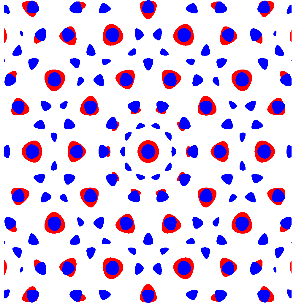
Figure 1: The stationary decagonal quasicrystal in the binary CMSH model. (a): The spatial distribution of density, where the red and blue colors correspond to the rich concentration of $\phi_{1}$ and $\phi_{2}$, respectively; (b): The Fourier spectra of $\phi_{1}$; (c): The Fourier spectra of $\phi_{2}$. Only Fourier spectral points whose coefficient intensities are larger than $10^{-4}$ are presented.

5.1.1 Algorithm study

In this subsection, we take the binary CMSH model as an example to show our proposed AB-BPG method’s performance by choosing different hyperparameters, including the choice of the step sizes, the descent subsequence, and the block update manner. Similar results exist in the following ternary and quinary cases. For simplicity, we only present the results in the computing binary CMSH model.

The step size of the AB-BPG methods is adaptively obtained by Algorithm 1. In our implementation, we set $\alpha_{0}=0.1$, $\varsigma=(\sqrt{5}-1)/2$, $\eta=10^{-12}$, $\alpha_{\min}=10^{-6}$ and $\alpha_{\max}=10$ in Algorithm 1. Figure 2 (a) illustrates the adaptive step sizes versus the iteration when $M=0$ and $a=1$.

In Figure 2 (b), it shows the total energy of the sequence $\{\hat{\Phi}^{k}\}$ and the subsequence $\{\hat{\Phi}^{m_{k}}\}$ defined in (17) versus the iterations with $M=5$ and $a=0$. It is observed that the subsequence $\{E(\hat{\Phi}^{m_{k}}\})$ is monotone decreasing which validates the generalized energy dissipation property proved in Lemma 3.10.

In the next, we consider the different choices of the update blocks. One is the cyclic rule that updates $\hat{\Phi}_{1}$ and $\hat{\Phi}_{2}$ alternatively in the Gauss-Seidel fashion. The other is to randomly choose the update block, and $\hat{\Phi}_{1}$ and $\hat{\Phi}_{2}$ should be updated at least once in $10$ consecutive iterations. In this case, we set $a=M=0$, and we independently run the random update rule 50 times and report its terminated iteration numbers for each trial. The result is shown in Figure 2 (c). Compared to the random update manner, it is observed that the cyclic rule needs fewer iterations for the desired accuracy. Therefore, in the following simulations, we only consider the cyclic update order when carrying out the AB-BPG algorithms.

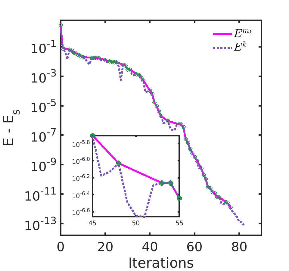
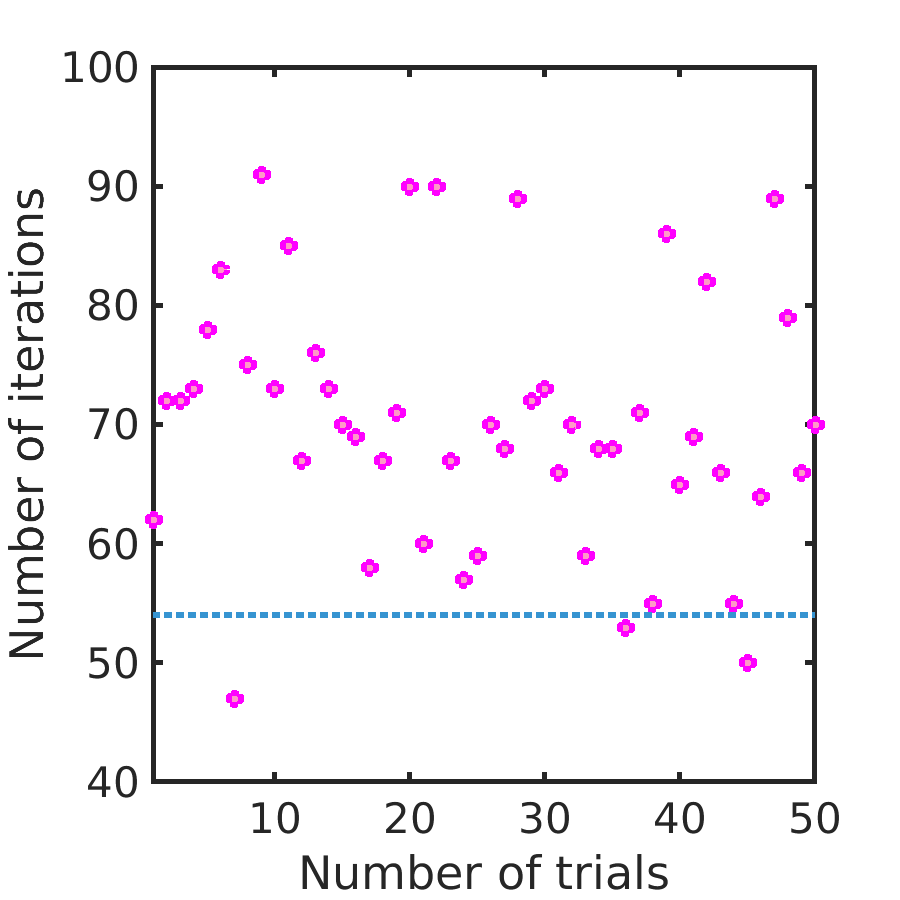
Figure 2: (a): The adaptive step size obtained by the AB-BPG-4 ($M=0$, $a=1$). The mean step sizes of $\phi_{1}$ and $\phi_{2}$ are $0.6033$ and $0.7062$, respectively. (b): The tendency of energy $\{E^{k}=E(\hat{\Phi}^{k})\}$ and energy $\{E^{m_{k}}=E(\hat{\Phi}^{m_{k}})\}$ in AB-BPG-2 ($M=5$, $a=0$). The green o’s mark the position of $(m_{k},E^{m_{k}})$. (c): Numerical behavior of the AB-BPG-2 ($M=0$, $a=0$) via updating order parameters in a random manner. The blue dotted line and the pink points denote the convergent iterations of the AB-BPG methods via cyclic and random order update, respectively.

5.1.2 Comparison with other methods

We compare AA-BPG methods with alternative methods, including adaptive SIS, adaptive BDF2, adaptive SAV and adaptive S-SAV. Theoretically, the SAV method always has a modified energy dissipation through adding a sufficiently large positive scalar auxiliary variable $C$ which guarantees the boundedness of the bulk energy term. In practice, the original energy dissipation property might depend on the selection of $C$. When computing the decagonal quasicrystal in the binary CMSH model, the adaptive SAV scheme keep the original energy dissipate when $C=10^{8}$. The times stepping for adaptive SAV scheme is obtained by formula (42) with $\alpha_{\min}=10^{-5}$, $\alpha_{\max}=0.5$, $\rho=0.9$, $\mathrm{tol}=10^{-3}$. For the AB-BPG approaches, we choose different values of $M$ in (17) and $a$ in Bregman divergence (37) for comparison. The linear search technique can obtain the step size of the AB-BPG methods.

Table 3 shows the corresponding numerical results of the AB-BPG, adaptive SIS, adaptive BDF2, adaptive SAV and adaptive S-SAV schemes. We choose a reference energy value $E_{s}=-1.54929536255898\times 10^{-2}$, which is computed via the semi-implicit scheme using $56^{4}$ plane wave functions. The minimal iteration steps and the least CPU time are emphasized via the bold font. From Table 3, one can find that the proposed approaches are superior to other methods. In particular, when $a=1$, the AB-BPG method with $M=0$ takes $45$ iterations ($69.17$ seconds) to reduce the gradient error of $10^{-7}$, which is $2.35$ times faster than the adaptive SIS, $4$ times than the adaptive BDF2 and adaptive SAV schemes, 10.73 times than the adaptive S-SAV scheme. Moreover, a great deal of the adaptive time stepping for gradient flow methods is that empirical parameters are involved in the formula (41) and (42), where the best-performing parameters usually cannot be guided in advance. Unsuitable choice of parameters may lead to too small step size (inefficient performance) or too large step size (divergence). While in our AB-BPG methods, efficient performances are shown in a wild range of choice of parameters. More importantly, the original energy dissipation and convergence are both guaranteed within any choice of parameters in our methods. Figure 3 presents the iteration process of relative energy difference, CPU time, and gradient error of different approaches.

Table 3: Numerical results of computing binary decagonal quasicrystal.

$M$	$a$	Iterations	CPU Time (s)	Gradient error ($10^{-8}$)	$|E-E_{s}|$ ($10^{-14}$)
	0	54	72.56	9.74	4.07
	0.1	46	66.04	9.42	51.54
0	1	45	69.17	7.95	13.78
	0	65	86.62	4.91	0.76
	0.1	59	85.10	9.25	23.08
5	1	57	82.79	7.99	18.62
	0	65	85.88	4.01	0.06
	0.1	59	85.31	9.60	95.61
10	1	56	79.38	7.13	2.98
Adaptive SIS		293	163.10	9.98	152.28
Adaptive BDF2		305	276.98	9.77	142.73
Adaptive SAV		94	283.14	8.86	117.56
Adaptive S-SAV		236	742.46	9.81	141.65

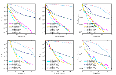
Figure 3: Numerical behaviors of our algorithms, adaptive SIS, adaptive BDF2, adaptive SAV, adaptive S-SAV for computing binary decagonal quasicrystal. First row: $M=0$; Second row: $M=5$; Left column: Relative energy over iterations; Middle column: Relative energy over CPU time; Right: Gradient error over iterations; The green $\times$s mark where restarts occurred.

5.2 Ternary component systems

We consider the ternary component system when $s=3$ in the CMSH model. A periodic structure of the sigma phase, which is a complicated spherical packed structure discovered in multicomponent material systems [31], is used to examine the performance of our algorithms. For such a pattern, we implement our algorithm on a bounded computational domain $[0,27.7884)\times[0,27.7884)\times[0,14.1514)$ and $200\times 200\times 100$ plane wave functions are used to for discretization. The initial value of each component of the sigma phase is input, as suggested in [51, 4]. The parameters in the ternary CMSH model are given in Table 4. The stationary sigma phase is present in Figure 4.

Table 4: The non-zero model parameters used in computing ternary sigma phase.

$c=1$, $q_{1}=q_{2}=q_{3}=1$, $\tau_{2,0,0}=\tau_{0,2,0}=\tau_{0,0,2}=-0.2$, $\tau_{3,0,0}=\tau_{0,3,0}=\tau_{0,0,3}=-0.3$, $\tau_{4,0,0}=\tau_{0,4,0}=\tau_{0,0,4}=0.1$, $\tau_{2,1,1}=\tau_{1,2,1}=\tau_{1,1,2}=-0.1$.

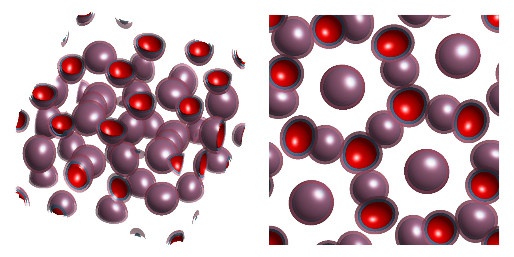
Figure 4: The stationary sigma phase in ternary CMSH model from two perspectives.

Similar to the binary case, we report the AB-BPG algorithms’ performance with different choices of $a$ and $M$. In the adaptive SAV method, the auxiliary parameter $C$ is set to $10^{8}$ and the parameters in formula (42) are chosen as $\alpha_{\min}=10^{-5}$, $\alpha_{\max}=0.2$, $\rho=0.8$, $\mathrm{tol}=10^{-3}$. Table 5 presents the corresponding numerical results and Figure 5 gives the iteration process of different methods. The reference energy value $E_{s}=-1.16910245253091$ is obtained numerically via semi-implicit scheme by using $256\times 256\times 128$ plane wave functions. As is evident from these results, the AB-BPG methods demonstrate a great advantage in computing such a complicated periodic structure over other schemes. More precisely, when $M=5$ and $a=1$, the AB-BPG method spends $416$ iterations to achieve the prescribed error, which converges $16.5$ times faster than the adaptive SIS and adaptive BDF2 methods, $3$ times than the adaptive SAV method and $6.5$ times than the adaptive S-SAV method. From the cost of CPU time, the AB-BPG algorithm with $M=5$, $a=1$ takes $1358.93$ seconds to achieve an accuracy of $10^{-7}$ in error, almost $10.7\%$, $10.8\%$, $11.9\%$ and $6.5\%$ the time employed by the adaptive SIS, adaptive BDF2, adaptive SAV and adaptive S-SAV schemes.

Table 5: Numerical results of computing ternary sigma phase.

$M$	$a$	Iterations	CPU Time (s)	Gradient error ($10^{-8}$)	$|E-E_{s}|$ ($10^{-12}$)
	0	758	2185.19	6.47	3.22
	0.1	770	2549.49	9.15	3.57
0	1	593	1952.63	9.71	4.79
	0	739	2068.65	9.50	3.54
	0.1	611	1991.94	8.23	2.01
5	1	416	1358.93	8.51	0.68
	0	677	1896.60	7.13	2.40
	0.1	595	1959.80	9.22	0.58
10	1	560	1865.38	7.32	1.31
Adaptive SIS		6905	12656.52	9.96	6.28
Adaptive BDF2		6896	12549.01	9.99	5.96
Adaptive SAV		1276	11406.12	9.94	6.11
Adaptive S-SAV		2737	20773.66	9.99	5.94

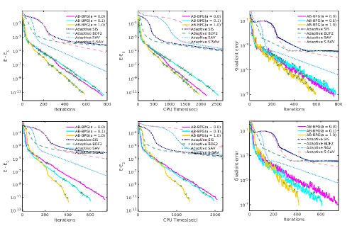
Figure 5: Numerical behaviors of the AB-BPG, adaptive SIS, adaptive BDF2, adaptive SAV and adaptive S-SAV algorithms for computing ternary sigma phase. First row: $M=0$; Second row: $M=20$; Left column: Relative energy over iterations; Middle column: Relative energy over CPU time; Right: Gradient error over iterations; The green $\times$s mark where restarts occurred.

5.3 Quinary component systems

The last multicomponent system considered in this paper is the five component CMSH model. We take a two-dimensional chessboard-shaped tiling phase and three-dimensional body-centered cubic (BCC) spherical structure to examine AB-BPG approaches’ performance.

5.3.1 Chessboard-shaped tiling

When computing the chessboard-shaped tiling, the parameters in five-component CMSH model are given in Table 6. The corresponding computational domain in physical space is $\Omega=[0,2\pi)^{2}$ and $1024\times 1024$ plane wave functions are used to discretize the computational domain. The initial solution of $j$-th component is

$$\phi_{j}(\bm{r})=\sum_{\bm{h}\in\Lambda_{0}^{j}}\hat{\phi}(\bm{h})e^{i\bm{h}^{\top}\bm{r}},~{}~{}\bm{r}\in\Omega,$$ (44)

where initial lattice points set $\Lambda_{0}^{j}\subset\mathbb{Z}^{2}$ can be found in the Table 7 only on which the Fourier coefficients $\hat{\phi}(\bm{h})$ located are nonzero. The convergent stationary morphology is given in Figure 6.

Table 6: The non-zero model parameters when computing quinary chessboard-shaped tiling.

$c=10$, $q_{1}=q_{2}=\cdots=q_{5}=1$, $\tau_{3,0,0,0,0}=\tau_{0,3,0,0,0}=\tau_{0,0,3,0,0}=\tau_{0,0,0,3,0}=\tau_{0,0,0,0,3}=-0.10$, $\tau_{4,0,0,0,0}=\tau_{0,4,0,0,0}=\tau_{0,0,4,0,0}=\tau_{0,0,0,4,0}=\tau_{0,0,0,0,4}=0.10$, $\tau_{1,0,1,0,0}=-0.70$, $\tau_{0,1,0,1,1}=0.05$, $\tau_{1,1,0,0,1}=-0.12$, $\tau_{0,1,0,1,0}=-0.44$.

Table 7: The initial lattice points of each component when computing quinary chessboard-shaped tiling.

	$\phi_{1}$	$\phi_{2}$	$\phi_{3}$	$\phi_{4}$	$\phi_{5}$
$\Lambda_{0}^{j}$	$(\pm 1,0)$	$(0,\pm 1)$	$(\pm 2,0)$	$(0,\pm 2)$	$(0,0)$

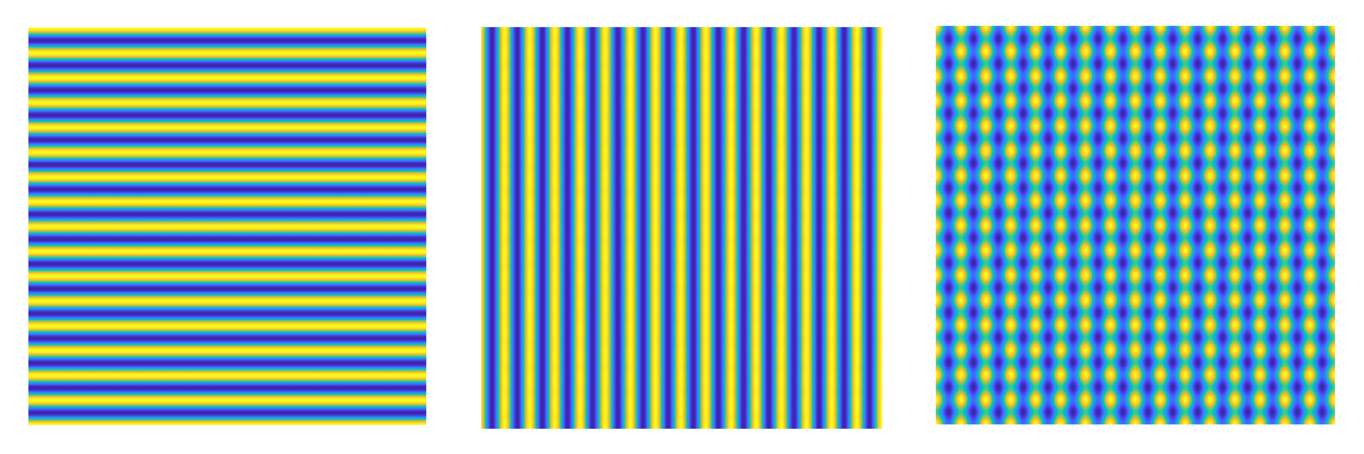
Figure 6: The stationary chessboard-shaped phase in quinary CMSH model. The morphologies of $\phi_{1},\phi_{3}$ (Left), $\phi_{2},\phi_{4}$ (Middle) and $\phi_{5}$ (Right).

Table 8 presents the numerical results of the AB-BPG, adaptive SIS, adaptive BDF2, adaptive SAV and adaptive S-SAV methods. The scalar auxiliary parameter $C$ of adaptive SAV scheme is set to $10^{10}$ and the parameters in formula (42) are taken as $\alpha_{\min}=10^{-5}$, $\alpha_{\max}=0.7$, $\rho=0.9$, $\mathrm{tol}=10^{-3}$. The reference energy value $E_{s}=-0.57163687783216$ is obtained via semi-implicit scheme by using $2048\times 2048$ plane wave functions. Correspondingly, Figure 7 presents the iteration process including the relative energy difference, the CPU times and the gradient error against iterations, respectively. These results demonstrate the superiority of the AB-BPG algorithms over the adaptive SIS, adaptive BDF2 and adaptive SAV methods. As Table 8 shows, the AB-BPG method with $M=0$, $a=0$ has the best performance. Even though the AB-BPG method costs much time as the adaptive SIS and adaptive BDF2 approaches per iteration due to the linear search technique, its adaptive step size compensates the extra work converging to $10^{-7}$, almost $0.8\%$, $0.9\%$, $3.5\%$ and $0.4\%$ of CPU time spent by the adaptive SIS, adaptive BDF2, adaptive SAV methods, and adaptive S-SAV, respectively.

Table 8: Numerical results of computing the quinary chessboard-shape tiling

$M$	$a$	Iterations	CPU Time (s)	Gradient error ($10^{-8}$)	$|E-E_{s}|$ ($10^{-14}$)
	0	111	75.56	6.97	2.90
	0.1	142	101.52	5.44	1.48
0	1	204	145.30	6.60	1.19
	0	193	149.67	6.28	0.46
	0.1	174	131.11	9.65	1.38
5	1	239	171.46	9.91	1.72
	0	186	120.03	8.34	2.62
	0.1	188	135.34	6.56	0.84
10	1	253	186.38	5.37	0.52
Adaptive SIS		18208	8957.85	282.01	4617.51
Adaptive BDF2		17723	8277.81	346.25	7073.17
Adaptive SAV		927	2184.01	9.92	94.23
Adaptive S-SAV		6655	16131.94	9.99	94.51

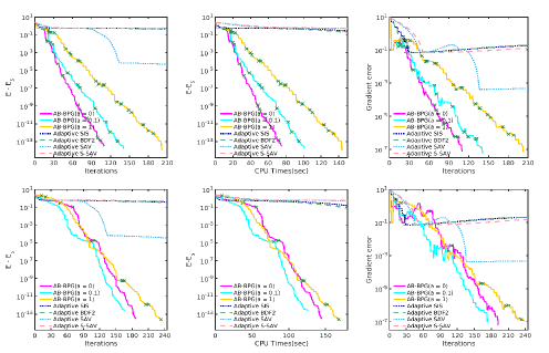
Figure 7: Numerical behaviors of the AB-BPG and adaptive SIS, adaptive BDF2, adaptive SAV and adaptive S-SAV for computing the quinary chessboard-shape tiling. First row: $M=0$; Second row: $M=5$; Left: Relative energy over iterations; Middle: Relative energy over CPU times; Right: Gradient error over iterations; The green $\times$s mark where restarts occurred.

5.3.2 BCC

As last, we consider the quinary BCC structure. The parameters in the five component CMSH model are given in Table 9. A bounded domain $[0,2\sqrt{2}\pi)^{3}$ is used as the computational box and $128^{3}$ plane wave functions are employed to compute the BCC spherical phase. The initial values can be found in [29]. Figure 8 shows the convergent stationary solution of different order parameter, which are all BCC phases but with different periodicity.

Table 9: The non-zero model parameters used in computing quinary BCC spherical structure.

$c=1$, $q_{1}=1$, $q_{2}=1.5$, $q_{3}=2$, $q_{4}=2.5$, $q_{5}=3$, $\tau_{3,0,0,0,0}=-0.1$, $\tau_{0,3,0,0,0}=-0.6$, $\tau_{0,0,3,0,0}=-0.4$, $\tau_{0,0,0,3,0}=-0.2$, $\tau_{0,0,0,0,3}=-0.1$, $\tau_{4,0,0,0,0}=\tau_{0,0,4,0,0}=\tau_{0,4,0,0,0}=\tau_{0,0,0,4,0}=\tau_{0,0,0,0,4}=0.1$, $\tau_{1,0,1,0,0}=0.4$, $\tau_{0,1,0,1,0}=0.3$, $\tau_{0,1,1,1,0}=-0.2$, $\tau_{1,1,0,0,1}=0.8$.

Table 10 and Figure 9 compare the numerical behaviors of AB-BPG, adaptive SIS, adaptive BDF2, adaptive SAV and adaptive S-SAV methods. The scalar auxiliary parameter $C$ of two SAV scheme is set to $10^{10}$. For adaptive SAV sheme, the parameters in formula (42) are taken as $\alpha_{\min}=10^{-5}$, $\alpha_{\max}=0.2$, $\rho=0.9$, $\mathrm{tol}=10^{-3}$. The reference energy $E_{s}=-1.22314417498279$ is obtained via semi-implicit scheme by using $256^{3}$ plane wave functions. Again, for this case, the proposed AB-BPG methods are still superior to the compared algorithms. More precisely, the best performance of AB-BPG ($M=0$, $a=0$) spends $182$ iterations to achieve the prescribed error which converges $40$ times faster than the adaptive SIS, $30$ times than the adaptive BDF2 method, $5.1$ times than the adaptive SAV scheme and $10.1$ times than the adaptive S-SAV scheme. From the cost of CPU times, the AB-BPG algorithm with $M=0$ takes $247.22$ seconds to achieve an accuracy of $10^{-7}$ in the gradient error, almost $3.8\%$, $5.1\%$, $7.0\%$ and $2.8\%$ of the CPU time used by the adaptive SIS, adaptive BDF2, adaptive SAV and adaptive S-SAV schemes.

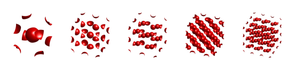
Figure 8: The stationary BCC phase in quinary CMSH model. The subfigures from left to right are morphology of $\phi_{1}$ to $\phi_{5}$.

Table 10: Numerical results of computing the quinary BCC structure

$M$	$a$	Iterations	CPU Times	Gradient error ($10^{-8}$)	$|E-E_{s}|$ ($10^{-13}$)
	0	182	247.22	8.17	1.99
	0.1	212	309.12	9.58	1.71
0	1	232	344.20	6.66	1.38
	0	259	343.63	3.96	1.37
	0.1	262	381.79	5.70	2.14
5	1	347	515.89	5.84	1.28
	0	277	371.94	5.56	1.33
	0.1	304	446.41	8.04	1.40
10	1	353	505.98	7.38	1.33
Adaptive SIS		7443	6446.39	52.18	439.44
Adaptive BDF2		5628	4802.81	71.90	832.20
Adaptive SAV		933	3498.08	9.94	17.20
Adaptive S-SAV		2204	8766.82	9.95	17.19

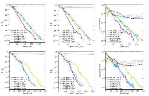
Figure 9: Numerical behaviors of the AB-BPG, adaptive SIS and adaptive BDF2, adaptive SAV and adaptive S-SAV methods for computing the quinary BCC phase. First row: $M=0$; Second row: $M=5$; Left: Relative energy over iterations; Middle: Relative energy over the CPU times; Right: Gradient error over iterations; The green $\times$s mark where restarts occurred.

6 Conclusion

In this paper, an AB-BPG algorithm is proposed to compute the stationary states of multicomponent phase-field crystal model with mass conservation. Compared to most existing methods, the new approaches consider the block structure of multicomponent models, and the update manner can be chosen deterministically or randomly. Using modern optimization methods, including the inertia acceleration approach, the restart technique, and the line search method, the proposed AB-BPG method has the general dissipation property with efficient implementation. Moreover, with the help of the Bregman divergence, it is proved that the generated sequence converges to a stationary point without the requirement of the global Lipschitz assumption. Extensive numerical experiments on computing stationary periodic crystals and quasicrystals in the binary, ternary, and quinary coupled-mode Swift-Hohenberg model have shown a significant acceleration over many existing methods.

In this paper, we have implemented our algorithms for computing multicomponent model with polynomial type potentials $F[\{\phi_{j}\}_{j=1}^{s}]$. In fact, the proposed methods can be applied to deal with non-polynomial type potentials by choosing suitable $\{h_{j}\}$ to make our Assumption 2 satisfied. This will soon be found in our future work. Besides, although our methods have shown efficient performance in our numerical experiments, we want to theoretically prove the convergence rates in the future. It is worth mentioning that in this work, we only consider efficient methods for computing stationary states. Besides, the physical evolution simulation is an important topic in PFC models. It is known that the classical proximal gradient method is exactly the semi-implicit scheme for gradient flows. From this perspective, we will develop our method to simulate the whole evolution of process of crystal growth in the further.

Appendix A: Projection method

The projection method is a general framework to study the periodic and quasiperiodic crystals [30, 25]. Each of the $d$-dimensional periodic system can be described by a Bravais lattice

$$\mathcal{R}_{d}=\{\bm{A}_{d}\bm{n}_{d},~{}\bm{n}_{d}\in\mathbb{Z}^{d}\},$$

where $\bm{A}_{d}\in\mathbb{R}^{d\times d}$ is invertible. The fundamental domain or so-called unit cell of the periodic system is

$$\Omega=\{\bm{A}_{d}\bm{\zeta},~{}\bm{\zeta}\in\mathbb{R}^{d},~{}\zeta_{j}\in[0,1),~{}j=1,\dots,d\}.$$

The associated primitive reciprocal vectors, $\bm{B}_{d}=(\bm{b}_{1},\dots,\bm{b}_{d})$, $\bm{b}_{j}\in\mathbb{R}^{d}$, $j=1,\dots,d$, satisfy the dual relationship $\bm{A}_{d}\bm{B}_{d}^{T}=\bm{I}_{d}$ where $\bm{I}_{d}$ is the $d$-order identify matrix. The reciprocal lattice is

$$\mathcal{R}^{*}_{d}=\{\bm{B}_{d}\bm{h}_{d},~{}\bm{h}_{d}\in\mathbb{Z}^{d}\}.$$

The corresponding periodic function $\psi(\bm{r})$, which has translational invariance with respect to the Bravais lattice $\mathcal{R}$, i.e., $\psi(\bm{r})=\psi(\bm{r}+\mathcal{R})$, has the following Fourier expansion

$$\psi(\bm{r})=\sum_{\bm{h}\in\mathbb{Z}^{d}}\hat{\psi}(\bm{h})e^{i(\bm{B}\bm{h})^{T}\bm{r}},$$ (45)

where

$$\hat{\psi}(\bm{h})={\mathchoice{{-\mkern-19.0mu\int}}{{-\mkern-16.0mu\int}}{{-\mkern-16.0mu\int}}{{-\mkern-16.0mu\int}}}\psi(\bm{r})e^{-(\bm{B}\bm{h})^{T}\bm{r}}d\bm{r},\quad\bm{r}\in\Omega.$$ (46)

Quasiperiodic functions, or more general almost periodic functions, are an extension of periodic functions. The definition of quasiperiodic functions is given as follows [25]:

Definition 6.1 (Quasiperiodic function).

A $d$-dimensional continuous complex-valued function $f(\bm{r})$ is quasiperiodic, if there exists a $n$-dimensional periodic function $F(\bm{r}_{s})$, $\bm{r}_{s}\in\mathbb{R}^{n}$, $n\geqslant d$, such that

$$f(\bm{r})=F(\mathcal{P}^{T}\bm{r}),$$

where $\mathcal{P}\in\mathbb{R}^{d\times n}$ is the projection matrix. The column vectors of $\mathcal{P}$ are rationally independent.

From the definition, one can find that the $d$-dimensional quasiperiodic system is a $d$-dimensional subspace of a $n$-dimensional periodic structure. As describes above, the Fourier series of $F(\bm{r}_{s})$ is

$$F(\bm{r}_{s})=\sum_{\bm{h}\in\mathbb{Z}^{n}}\hat{F}(\bm{h})e^{i(\bm{B}\bm{h})^{T}\bm{r}_{s}},$$ (47)

where $\bm{B}\in\mathbb{R}^{n\times n}$ is associated to the periodicity of the $n$-dimensional periodic system. $\hat{F}(\bm{h})={\mathchoice{{-\mkern-19.0mu\int}}{{-\mkern-16.0mu\int}}{{-\mkern-16.0mu\int}}{{-\mkern-16.0mu\int}}}F(\bm{r}_{s})e^{-(\bm{B}\bm{h})^{T}\bm{r}_{s}}\,d\bm{r}_{s},\,\bm{r}_{s}\in\Omega_{s}$, $\Omega_{s}=\{\bm{B}^{-T}\bm{\alpha},~{}\bm{\alpha}\in\mathbb{R}^{n},~{}\alpha_{j}\in[0,1),~{}j=1,\ldots,n\}$. Let $\hat{F}(\bm{h})$ be $\hat{f}(\bm{h})$, the projection method for a $d$-dimensional quasiperiodic function over $\mathbb{R}^{d}$ can be written as [30]

$$f(\bm{r})=\sum_{\bm{h}\in\mathbb{Z}^{n}}\hat{f}(\bm{h})e^{i(\mathcal{P}\bm{B}\bm{h})^{\top}\bm{r}},\quad\bm{r}\in\mathbb{R}^{d}.$$ (48)

If consider periodic crystals, the projection matrix becomes the $d$-order identity matrix, then the projection reduces to the common Fourier spectral method.

Similarly, the order parameter in multicomponent systems can be expanded as follows

$$\phi_{j}(\bm{r})=\sum_{\bm{h}\in\mathbb{Z}^{n}}\hat{\phi}_{j}(\bm{h})e^{i(\mathcal{P}\bm{B}\bm{h})^{\top}\bm{r}},\quad j=1,2,\cdots,s.$$ (49)

In numerical implementation, we truncate the Fourier coefficients to satisfy

$$X_{j}=\{\{\hat{\phi}_{j}(\bm{h})\}_{\bm{h}\in\mathbb{Z}^{n}}:\hat{\phi}_{j}(\bm{h})=0,~{}\forall\,|h_{l}|>\dfrac{N_{l,j}}{2},~{}l=1,2,\cdots,n\}.$$

where $N_{l,j}$ is chosen to be even for convenience. Let $\bm{\hat{\phi}}_{j}=(\hat{\phi}_{1,j},\hat{\phi}_{2,j},\cdots,\hat{\phi}_{\bm{N}_{j},j})^{\top}\in\mathbb{C}^{N_{j}}$ with $\bm{N}_{j}=\prod_{l=1}^{n}(N_{l,j}+1)$. Let $\hat{\Phi}=\{\bm{\hat{\phi}}_{j}\}_{j=1}^{s}\in\mathbb{C}^{\bm{N}}$ with $\bm{N}=\sum_{j=1}^{s}\bm{N}_{j}$. Using the projection method discretization, the energy functional (6) reduce to

$$G_{\bm{h},j}(\bm{\hat{\phi}}_{j}) =\frac{1}{2}\sum_{\bm{h}_{j,1}+\bm{h}_{j,2}=0}\left[q_{j}^{2}-(\mathcal{P}\mathbf{B}\bm{h})^{\top}(\mathcal{P}\mathbf{B}\bm{h})\right]^{2}\hat{\phi}_{j}(\bm{h}_{j,1})\hat{\phi}_{j}(\bm{h}_{j,2}),\quad j=1,2,\dots,s,$$

$$F_{\bm{h}}(\hat{\Phi}) =\sum_{\mathcal{I}_{s,n}}\tau_{i_{1},i_{2},\cdots,i_{s}}\sum_{\sum_{j,k}\bm{h}_{j,k}=0}\prod_{j=1}^{s}\left(\prod_{k=1}^{i_{j}}\hat{\phi}_{j}(\bm{h}_{j,k})\right),$$

where $\bm{h}_{j,k}\in\mathbb{Z}^{n}$, $\hat{\phi}_{j}\in X_{j}$, $j=1,2,\dots,s$. For simplicity, we omit the subscription $\bm{h}$ in $G_{\bm{h},j}$ and $F_{\bm{h}}$ in the following context. Then the discretized energy functional can be stated as

$$\begin{split}E(\{\bm{\hat{\phi}}_{j}\}_{j=1}^{s})=\sum_{j=1}^{s}G_{j}(\bm{\hat{\phi}}_{j})+F(\{\bm{\hat{\phi}}_{j}\}_{j=1}^{s}),\end{split}$$ (50)

where $G_{j}(\bm{\hat{\phi}}_{j})=\dfrac{1}{2}\langle\bm{\hat{\phi}}_{j},\mathcal{D}_{j}\bm{\hat{\phi}}_{j}\rangle$ and $\mathcal{D}_{j}\in\mathbb{C}^{\bm{N}_{j}\times\bm{N}_{j}}$ is a diagonal matrix with nonnegative entries

$$(\mathcal{D}_{j})_{\bm{h}}=[q_{j}^{2}-(\mathcal{P}\bm{B}\bm{h})^{\top}(\mathcal{P}\bm{B}\bm{h})]^{2}\text{ with }\bm{h}\in\mathbb{Z}^{n}\text{ and }\hat{\phi}_{j}(\bm{h})\in X_{j}.$$ (51)

$F(\{\bm{\hat{\phi}}_{j}\}_{j=1}^{s})$ are $n$-dimensional convolutions in the reciprocal space. In summary, the discretized version of (7) has the form

$$\begin{split}\min_{\hat{\Phi}}~{}E(\hat{\Phi})=\sum_{j=1}^{s}G_{j}(\bm{\hat{\phi}}_{j})+F(\hat{\Phi}),\quad\mathrm{s.t.}\quad e_{1}^{\top}\bm{\hat{\phi}}_{j}=0,\quad j=1,2,\cdots,s.\end{split}$$ (52)

Appendix B: Proof of Theorem 5

Before we prove the convergent property, we first present a useful lemma for our analysis.

Lemma 6.2 (Uniformized Kurdyka-Lojasiewicz property [10].).

Let $\mathcal{C}$ be a compact set and $E$ defined in (8) be bounded below. Assume that $E$ is constant on $\mathcal{C}$. Then, there exist $\epsilon>0$, $\eta>0$, and $\psi\in\Psi_{\eta}$ such that for all $\bar{u}\in\mathcal{C}$ and all $u\in\Gamma_{\eta}(\bar{u},\epsilon)$, one has,

$$\psi^{{}^{\prime}}(E(u)-E(\bar{u}))\mathrm{dist}(\bm{0},\partial E(u))\geq 1,$$ (53)

where $\Psi_{\eta}=\{\psi\in C[0,\eta)\cap C^{1}(0,\eta)\text{and }\psi\text{is concave},\psi(0)=0,\psi^{{}^{\prime}}>0\text{on }(0,\eta)\}$ and $\Gamma_{\eta}(x,\epsilon)=\{y|\|x-y\|\leq\epsilon,E(x)<E(y)<E(x)+\eta\}$.

Proof 6.3.

The proof is based on the fact that $E$ satisfies the so-called Kurdyka-Lojasiewicz property on $\mathcal{C}$ [10].

Proof of Theorem 5

Proof 6.4.

Define two sets $\Omega_{2}=\{k\,|\,w_{k}=0\}$ and $\Omega_{1}=\mathbb{N}\backslash\Omega_{2}$. Since $M=0$, we know $m_{k}\equiv k$. From the restart technique (18), the following sufficient decrease property holds

$$E(X^{k})-E(X^{k+1})\geq\sigma\|X^{k}-X^{k+1}\|^{2},~{}\forall k.$$ (54)

Let $S(X^{0})$ be the set of limiting points of the sequence $\{X^{k}\}$ starting from $X^{0}$. By the boundedness of $\{X^{k}\}$ and $S(X^{k})=\cap_{n\in\mathbb{N}}\cup_{k\geq n}\{X^{k}\}$, it follows that $\{X^{k}\}$ is a non-empty and compact set. From Lemma 3.15, we know

$$E(X)=E^{*},\quad\forall X\in S(X^{0}).$$ (55)

Then, for all $\varepsilon_{1},\eta>0$, there exists $k_{0}>0$ such that

$$\mathrm{dist}(X^{k},S(X^{0}))\leq\varepsilon_{1},\quad E^{*}<E(X^{k})<E^{*}+\eta,\quad\forall k>k_{0}.$$ (56)

Applying Lemma 53, for $\forall k>k_{0}$ we have

$$\psi^{\prime}(E(X^{k})-E^{*})\mathrm{dist}(\bm{0},\partial E(X^{k}))\geq 1.$$ (57)

By the convexity of $\psi$, we have

$$\psi(E(X^{k})-E^{*})-\psi(E(X^{k+1})-E^{*})\geq\psi^{\prime}(E(X^{k})-E^{*})(E(X^{k})-E(X^{k+1})).$$ (58)

Denote $\Delta_{k,k+1}=\psi(E(X^{k})-E^{*})-\psi(E(X^{k+1})-E^{*})$. From (54), we have

$$\Delta_{k,k+1}\geq\dfrac{\sigma\|X^{k+1}-X^{k}\|^{2}}{\mathrm{dist}(\bm{0},\partial E(X^{k}))},\quad\forall k>k_{0}$$ (59)

Next, we prove $\sum_{k=0}^{\infty}\|X^{k+1}-X^{k}\|<\infty$. For any $\varepsilon>0$, we take $N>\max\{k_{0},3T\}$ large enough such that

$$\bar{C}\psi(E(X^{N+1})-E^{*})<\varepsilon/2,$$ (60)

$$\sum_{k=N-3T+2}^{N}\|X^{k+1}-X^{k}\|<\varepsilon/2,$$ (61)

where $\bar{C}=3TC/\sigma$. The existence of $N$ is ensured by the fact that $\lim\limits_{k\rightarrow\infty}E(X^{k})=E^{*}$, $\psi(0)=0$ and $\lim\limits_{k\rightarrow\infty}\|X^{k+1}-X^{k}\|=0$. We now show that for all $\forall K>N$, the following inequality holds

$$\sum_{k=N+1}^{K}\|X^{k+1}-X^{k}\|<\varepsilon,$$ (62)

which implies $\sum_{k=0}^{\infty}\|X^{k+1}-X^{k}\|<\infty$ by Cauchy principle of convergence. In fact, together with Lemma 3.18 and (59), we obtain

$$\Delta_{k,k+1}\geq\dfrac{\|X^{k+1}-X^{k}\|^{2}}{C_{1}\sum_{l=k-3T+1}^{k}\|X^{l}-X^{l-1}\|},\quad\forall k>N$$ (63)

where $C_{1}=C/\sigma.$ By using the geometric inequality, we get

$$2\|X^{k+1}-X^{k}\|\leq\dfrac{1}{3T}\sum_{l=k-3T+1}^{k}\|X^{l}-X^{l-1}\|+\bar{C}\Delta_{k,k+1},$$ (64)

Summing up (64) for $k=N+1,\cdots,K$, it follows that

$$2\sum_{k=N+1}^{K}\|X^{k+1}-X^{k}\| \leq\sum_{k=N+1}^{K}\left(\dfrac{1}{3T}\sum_{l=k-3T+1}^{k}\|X^{l}-X^{l-1}\|+\bar{C}\Delta_{k,k+1}\right)$$

$$=\dfrac{1}{3T}\sum_{k=N+1}^{K}\sum_{l=-3T+1}^{0}\|X^{l+k}-X^{l+k-1}\|+\bar{C}\Delta_{N+1,K+1}$$

$$=\dfrac{1}{3T}\sum_{l=-3T+1}^{0}\sum_{k=N+l+1}^{K+l}\|X^{k}-X^{k-1}\|+\bar{C}\Delta_{N+1,K+1}$$

$$\leq\dfrac{1}{3T}\sum_{l=-3T+1}^{0}\sum_{k=N-3T+2}^{K}\|X^{k}-X^{k-1}\|+\bar{C}\Delta_{N+1,K+1}$$

$$=\sum_{k=N-3T+2}^{K}\|X^{k}-X^{k-1}\|+\bar{C}\Delta_{N+1,K+1}$$

$$\leq\sum_{k=N-3T+1}^{K}\|X^{k+1}-X^{k}\|+\bar{C}\Delta_{N+1,K+1},$$

where the first equality is from the fact that $\Delta_{p,q}+\Delta_{q,r}=\Delta_{p,r}$. Therefore, we have

$$\sum_{k=N+1}^{K}\|X^{k+1}-X^{k}\|\leq\sum_{k=N-3T+1}^{N}\|X^{k+1}-X^{k}\|+\bar{C}\psi(E(X^{N+1})-E^{*})<\varepsilon$$ (65)

As a result, we obtain $\sum_{k=0}^{\infty}\|X^{k+1}-X^{k}\|<\infty$ and $\lim\limits_{k\rightarrow\infty}X^{k}=X^{*}$. From Lemma 3.15 and the continuity of $E(X)$ on $\mathcal{B}(X^{0})$, we get

$$\lim\limits_{k\rightarrow\infty}E(X^{k})=E(X^{*})=E^{*}.$$ (66)

References

- [1] Masoud Ahookhosh, Le Thi Khanh Hien, Nicolas Gillis, and Panagiotis Patrinos. Multi-block Bregman proximal alternating linearized minimization and its application to sparse orthogonal nonnegative matrix factorization. arXiv preprint arXiv:1908.01402, 2019.
- [2] Eli Alster, KR Elder, Jeffrey J Hoyt, and Peter W Voorhees. Phase-field-crystal model for ordered crystals. Physical Review E, 95(2):022105, 2017.
- [3] Eli Alster, David Montiel, Katsuyo Thornton, and Peter W Voorhees. Simulating complex crystal structures using the phase-field crystal model. Physical Review Materials, 1(6):060801, 2017.
- [4] Akash Arora, Jian Qin, David C Morse, Kris T Delaney, Glenn H Fredrickson, Frank S Bates, and Kevin D Dorfman. Broadly accessible self-consistent field theory for block polymer materials discovery. Macromolecules, 49(13):4675–4690, 2016.
- [5] Vittorio E Badalassi, Hector D Ceniceros, and Sanjoy Banerjee. Computation of multiphase systems with phase field models. Journal of Computational Physics, 190(2):371–397, 2003.
- [6] Chenglong Bao, Hui Ji, Yuhui Quan, and Zuowei Shen. Dictionary learning for sparse coding: Algorithms and convergence analysis. IEEE Transactions on Pattern Analysis and Machine Intelligence, 38(7):1356–1369, 2015.
- [7] Jonathan Barzilai and Jonathan M Borwein. Two-point step size gradient methods. IMA Journal of Numerical Analysis, 8(1):141–148, 1988.
- [8] Heinz H Bauschke, Jérôme Bolte, and Marc Teboulle. A descent lemma beyond Lipschitz gradient continuity: First-order methods revisited and applications. Mathematics of Operations Research, 42(2):330–348, 2016.
- [9] Heinz H Bauschke, Patrick L Combettes, et al. Convex Analysis and Monotone Operator Theory in Hilbert Spaces, volume 408. Springer, 2011.
- [10] Jérôme Bolte, Shoham Sabach, and Marc Teboulle. Proximal alternating linearized minimization for nonconvex and nonsmooth problems. Mathematical Programming, 146(1-2):459–494, 2014.
- [11] Franck Boyer and Sebastian Minjeaud. Numerical schemes for a three component Cahn-Hilliard model. ESAIM: Mathematical Modelling and Numerical Analysis, 45(4):697–738, 2011.
- [12] SA Brazovskiǐ. Phase transition of an isotropic system to a nonuniform state. Soviet Journal of Experimental and Theoretical Physics, 41:85, 1975.
- [13] Haim Brezis. Functional Analysis, Sobolev Spaces and Partial Differential Equations. Springer Science & Business Media, 2010.
- [14] Long-Qing Chen. Phase-field models for microstructure evolution. Annual Review of Materials Research, 32(1):113–140, 2002.
- [15] Wenbin Chen, Cheng Wang, Shufen Wang, Xiaoming Wang, and Steven M Wise. Energy stable numerical schemes for ternary Cahn-Hilliard system. J. Sci. Comput., 84:27, 2020.
- [16] Mark C Cross and Pierre C Hohenberg. Pattern formation outside of equilibrium. Reviews of Modern Physics, 65(3):851, 1993.
- [17] Qiang Du, Lili Ju, Xiao Li, and Zhonghua Qiao. Maximum principle preserving exponential time differencing schemes for the nonlocal Allen–Cahn equation. SIAM Journal on Numerical Analysis, 57(2):875–898, 2019.
- [18] Qiang Du, Lili Ju, Xiao Li, and Zhonghua Qiao. Maximum bound principles for a class of semilinear parabolic equations and exponential time-differencing schemes. SIAM Review, 63(2):317–359, 2021.
- [19] K. R. Elder, Nikolas Provatas, Joel Berry, Peter Stefanovic, and Martin Grant. Phase-field crystal modeling and classical density functional theory of freezing. Phys. Rev. B, 75:064107, Feb 2007.
- [20] KR Elder and Martin Grant. Modeling elastic and plastic deformations in nonequilibrium processing using phase field crystals. Physical Review E, 70(5):051605, 2004.
- [21] KR Elder, Mark Katakowski, Mikko Haataja, and Martin Grant. Modeling elasticity in crystal growth. Physical Review Letters, 88(24):245701, 2002.
- [22] Charles M Elliott and AM Stuart. The global dynamics of discrete semilinear parabolic equations. SIAM Journal on Numerical Analysis, 30(6):1622–1663, 1993.
- [23] Harald Garcke, Britta Nestler, and Barbara Stoth. A multiphase field concept: Numerical simulations of moving phase boundaries and multiple junctions. SIAM Journal on Applied Mathematics, 60(1):295–315, 1999.
- [24] Michael Greenwood, Nana Ofori-Opoku, Jörg Rottler, and Nikolas Provatas. Modeling structural transformations in binary alloys with phase field crystals. Phys. Rev. B, 84:064104, Aug 2011.
- [25] K. Jiang and P. Zhang. Numerical mathematics of quasicrystals. Proc. Int. Cong. of Math., 3:3575–3594, 2018.
- [26] Kai Jiang and Wei Si. Stability of three-dimensional icosahedral quasicrystals in multi-component systems. Philosophical Magazine, 100(1):84–109, 2020.
- [27] Kai Jiang, Wei Si, Chang Chen, and Chenglong Bao. Efficient numerical methods for computing the stationary states of phase field crystal models. SIAM Journal on Scientific Computing, 42(6):B1350–B1377, 2020.
- [28] Kai Jiang, Jiajun Tong, and Pingwen Zhang. Stability of soft quasicrystals in a coupled-mode Swift-Hohenberg model for three-component systems. Communications in Computational Physics, 19(3):559–581, 2016.
- [29] Kai Jiang, Chu Wang, Yunqing Huang, and Pingwen Zhang. Discovery of new metastable patterns in diblock copolymers. Communications in Computational Physics, 14(2):443–460, 2013.
- [30] Kai Jiang and Pingwen Zhang. Numerical methods for quasicrystals. Journal of Computational Physics, 256(1):428–440, 2014.
- [31] Sangwoo Lee, Michael J Bluemle, and Frank S Bates. Discovery of a Frank-Kasper phase in sphere-forming block copolymer melts. Science, 330(6002):349, 2010.
- [32] Jingwei Li, Xiao Li, Lili Ju, and Xinlong Feng. Stabilized integrating factor runge–kutta method and unconditional preservation of maximum bound principle. SIAM Journal on Scientific Computing, 43(3):A1780–A1802, 2021.
- [33] Qiuwei Li, Zhihui Zhu, Gongguo Tang, and Michael B Wakin. Provable Bregman-divergence based methods for nonconvex and non-Lipschitz problems. arXiv preprint arXiv:1904.09712, 2019.
- [34] Xin Liu, Zaiwen Wen, Xiao Wang, Michael Ulbrich, and Yaxiang Yuan. On the analysis of the discretized Kohn–Sham density functional theory. SIAM Journal on Numerical Analysis, 53(4):1758–1785, 2015.
- [35] Zhaosong Lu and Lin Xiao. Randomized block coordinate non-monotone gradient method for a class of nonlinear programming. arXiv preprint arXiv:1306.5918, 1273, 2013.
- [36] ND Mermin and Sandra M Troian. Mean-field theory of quasicrystalline order. Physical Review Letters, 54(14):1524, 1985.
- [37] Britta Nestler and Abhik Choudhury. Phase-field modeling of multi-component systems. Current Opinion in Solid State and Materials Science, 15(3):93–105, 2011.
- [38] Britta Nestler, Harald Garcke, and Björn Stinner. Multicomponent alloy aolidification: Phase-field modeling and simulations. Physical Review E, 71(4):041609, 2005.
- [39] Nana Ofori-Opoku, Vahid Fallah, Michael Greenwood, Shahrzad Esmaeili, and Nikolas Provatas. Multicomponent phase-field crystal model for structural transformations in metal alloys. Physical Review B, 87(13):134105, 2013.
- [40] Michael JD Powell. On search directions for minimization algorithms. Mathematical Programming, 4(1):193–201, 1973.
- [41] Zhonghua Qiao, Zhengru Zhang, and Tao Tang. An adaptive time-stepping strategy for the molecular beam epitaxy models. SIAM Journal on Scientific Computing, 33(3):1395–1414, 2011.
- [42] Samuel Savitz, Mehrtash Babadi, and Ron Lifshitz. Multiple-scale structures: from faraday waves to soft-matter quasicrystals. IUCrJ, 5(3), 2018.
- [43] Jie Shen, Jie Xu, and Jiang Yang. The scalar auxiliary variable (SAV) approach for gradient flows. Journal of Computational Physics, 353:407–416, 2018.
- [44] Jie Shen, Jie Xu, and Jiang Yang. A new class of efficient and robust energy stable schemes for gradient flows. SIAM Review, 61(3):474–506, 2019.
- [45] Jie Shen and Xiaofeng Yang. Numerical approximations of Allen-Cahn and Cahn-Hilliard equations. Discrete and Continuous Dynamical Systems-A, 28(4):1669, 2010.
- [46] Ingo Steinbach. Phase-field model for microstructure evolution at the mesoscopic scale. Annual Review of Materials Research, 43:89–107, 2013.
- [47] Ju Swift and Pierre C Hohenberg. Hydrodynamic fluctuations at the convective instability. Physical Review A, 15:319–328, Jan 1977.
- [48] Doaa Taha, SR Dlamini, SK Mkhonta, KR Elder, and Zhi-Feng Huang. Phase ordering, transformation, and grain growth of two-dimensional binary colloidal crystals: A phase field crystal modeling. Physical Review Materials, 3(9):095603, 2019.
- [49] Steven M Wise, Cheng Wang, and John S Lowengrub. An energy-stable and convergent finite-difference scheme for the phase field crystal equation. SIAM Journal on Numerical Analysis, 47:2269, 2009.
- [50] Xinming Wu, Zaiwen Wen, and Weizhu Bao. A regularized Newton method for computing ground states of Bose–Einstein condensates. Journal of Scientific Computing, 73(1):303–329, 2017.
- [51] Nan Xie, Weihua Li, Feng Qiu, and An-Chang Shi. phase formed in conformationally asymmetric AB-type block copolymers. Acs Macro Letters, 3(9):906–910, 2014.
- [52] Chuanju Xu and Tao Tang. Stability analysis of large time-stepping methods for epitaxial growth models. SIAM Journal on Numerical Analysis, 44(4):1759–1779, 2006.
- [53] Yangyang Xu and Wotao Yin. A globally convergent algorithm for nonconvex optimization based on block coordinate update. Journal of Scientific Computing, 72(2):700–734, 2017.
- [54] Xiaofeng Yang, Jia Zhao, Qi Wang, and Jie Shen. Numerical approximations for a three-component Cahn–Hilliard phase-field model based on the invariant energy quadratization method. Mathematical Models and Methods in Applied Sciences, 27(11):1993–2030, 2017.
- [55] Zhengru Zhang, Yuan Ma, and Zhonghua Qiao. An adaptive time-stepping strategy for solving the phase field crystal model. Journal of Computational Physics, 249:204–215, 2013.
- [56] Liyong Zhu, Lili Ju, and Weidong Zhao. Fast high-order compact exponential time differencing Runge–Kutta methods for second-order semilinear parabolic equations. Journal of Scientific Computing, 67(3):1043–1065, 2016.