The Race between Technology and Woman:
Changes in Gender and Skill Premia in OECD Countries

Abstract

The era of technological change entails complex patterns of changes in wages and employment. We develop a unified framework to measure the contribution of technological change embodied in new capital to changes in the relative wages and income shares of different types of labor. We obtain the aggregate elasticities of substitution by estimating and aggregating sectoral production function parameters with cross-country and cross-industry panel data from OECD countries. We show that advances in information, communication, and computation technologies contribute significantly to narrowing the gender wage gap, widening the skill wage gap, and declining labor shares.

Keywords: Gender wage gap; skill wage gap; labor share; capital–skill complementarity; capital-embodied technological change.
JEL classification: E23, E25, J16, J24, J31, O33.

1 Introduction

Over the decades, there have been substantial changes in the structure of wages and employment. The wage gap between male and female workers has narrowed in many countries, while that between skilled and unskilled workers has widened in some countries (Krueger, Perri, Pistaferri and Violante, 2010). At the same time, the share of labor in national income has declined in many countries (Karabarbounis and Neiman, 2014). During the period, there have been tremendous advances in information, communication, and computation technologies in industrialized nations. Such technological advances have been recognized as one of the causes for the widening of the skill wage gap and the decline in the labor share (Hornstein, Krusell and Violante, 2005; Acemoglu and Autor, 2011; Grossman and Oberfield, 2022).

The direction and magnitude of changes in the relative wages and income shares of different types of labor due to the introduction and expansion of technologically advanced new equipment depend on the presence and degree of capital–skill or capital–gender complementarity. Male and female workers possess different sets of skills (Welch, 2000), as skilled and unskilled workers do (Griliches, 1969). Communication skills, in which women can possibly have a comparative advantage, are more likely to be complementary to information and communication technologies. Physical skills, in which men can possibly have a comparative advantage, are more likely to be substitutable with computation and automation technologies. The widespread use of new technologies might raise the demand for brains relative to brawn, which could result in a narrowing of the gender wage gap, a widening of the skill wage gap, and a decline in the income share of male unskilled labor. However, in the literature, the analysis of the labor share has been conducted independently from that of wage inequality and has not been conducted separately by skill or gender.

This study develops a unified framework to measure the contribution of technological change embodied in new capital to changes in the relative wages and income shares of different types of labor. Our framework builds upon a multi-sector, multi-factor extension of the Greenwood, Hercowitz and Krusell (1997) model of investment-specific technological change. We incorporate technological change embodied in new capital into an economy consisting of multiple sectors, where multiple consumption and investment goods are produced from multiple types of capital and labor. The presence and degree of capital–skill and capital–gender complementarities in the multi-sector economy are determined by the aggregate elasticities of substitution among different types of capital and labor. We show that the aggregate elasticities of substitution are sufficient statistics to measure the contributions of specific factor inputs to aggregate changes in the relative wages and income shares of different types of labor. In this context, we generalize a model that explains changes in the wage premium to skill in terms of the race between technology and education (Tinbergen, 1974; Goldin and Katz, 2010) and a model that explains changes in the labor share in terms of capital deepening (Hicks, 1932; Elsby, Hobijn and Şahin, 2013). We further show that the aggregate elasticities of substitution are sufficient statistics to quantify the general equilibrium effects of capital-embodied technological change on the relative wages and income shares of different types of labor. In this context, we synthesize models that explain a rise in the skill premium or a decline in the labor share in terms of a fall in the relative price of capital equipment (Krusell, Ohanian, Rios-Rull and Violante, 2000; Karabarbounis and Neiman, 2014).

We apply this framework to developed economies consisting of multiple sectors, where the production of goods and services requires multiple types of capital and labor. Given the fact that capital-embodied technological progress was accelerated by information processing equipment and software in the 1980s and 1990s (Cummins and Violante, 2002), we distinguish equipment related to information, communication, and computation technologies from other types of capital. We refer to the former as ICT capital and the latter as non-ICT capital. We also distinguish between male skilled, female skilled, male unskilled, and female unskilled labor to examine the sources of changes in gender and skill premia. Although it is notoriously difficult to identify the elasticities of substitution in the aggregate production function using time-series data (Diamond, McFadden and Rodriguez, 1978), it is possible to obtain the aggregate elasticities of substitution by estimating and aggregating the disaggregated production function parameters with disaggregated data (Sato, 1975; Oberfield and Raval, 2021). An advantage of this approach is that it expands the choices of cross-sectional variation that we exploit to identify the elasticities of substitution.

We estimate the sectoral production function parameters and obtain the aggregate elasticities of substitution among the two types of capital and the four types of labor using cross-country and cross-industry data from OECD countries. We find that ICT equipment is more complementary not only to skilled labor than unskilled labor but also to female labor than male labor. The relative magnitude of the estimated elasticities of substitution is robust to the specification of the sectoral production function and to the presence of labor market institutions, factor-biased technological change, and markups. Our results suggest that the expansion of ICT equipment owing to technological progress contributes not only to the widening of the skill wage gap but also to the narrowing of the gender wage gap. Moreover, the expansion of ICT equipment contributes to a fall in the income share of male unskilled labor, which accounts for most of the decline in the labor share.

We show that technological change embodied in ICT equipment induces significant changes in the equilibrium relative wages and income shares of the four types of labor. On average in OECD countries, if all else were held constant, a fall in the relative price of ICT equipment between the years 1980 and 2005 would have reduced the skilled (unskilled) gender wage gap by 46 (7.5) percentage points and raised the male (female) skill wage gap by 26 (79) percentage points, while it would have raised the income share of male (female) skilled labor by 1.3 (1.9) percentage points and reduced the income share of male (female) unskilled labor by 6.0 (0.7) percentage points. However, whether the gender (skill) wage gap eventually narrows (widens) depends on the outcome of the race between progress in ICT and advances in female employment (educational attainment). We demonstrate that the observed difference in the rate of decrease (increase) in the gender (skill) wage gap by skill (gender) can also be explained in the same way.

The remainder of this paper is structured as follows. The next section reviews the related literature. Section 3 establishes the theoretical framework to estimate the aggregate elasticities of substitution among different types of capital and labor and to measure the contribution of technological change to aggregate changes in the relative wages and income shares of different types of labor. Section 4 discusses the specification, identification, estimation, and aggregation of parameters in the sectoral production function. Section 5 describes the data used in the analysis and shows changes in the relative prices, relative quantities, and income shares of factors. Section 6 presents the sectoral and aggregate results. The final section summarizes the main findings and concludes.

2 Related Literature

This study adds to several strands of literature. First, it is related to the literature on technological change and wage inequality. This strand of literature highlights the importance of factor-biased technological change in accounting for changes in wage inequality in the United States and OECD countries, typically by estimating the aggregate production function. The widening of the skill wage gap is attributed to skill-biased technological change (Bound and Johnson, 1992; Katz and Murphy, 1992; Goldin and Katz, 2010), technological change embodied in capital equipment (Krusell et al., 2000; Taniguchi and Yamada, 2022), or sector-specific disembodied technological change (Buera, Kaboski, Rogerson and Vizcaino, 2022). The narrowing of the gender wage gap is attributed to gender-biased technological change (Johnson and Keane, 2013).

Second, this study is related to the literature on the labor market impact of new technologies. This strand of literature indicates advances in information, communication, computation, and automation technologies as causes of changes in the structure of wages and employment in the United States and other OECD countries. The rate of increase in the wage bill share of skilled or female labor tends to be higher in ICT or computer-intensive industries (Autor, Katz and Krueger, 1998; Michaels, Natraj and Van Reenen, 2014; Raveh, 2015). The increased employment and wages of skilled or female labor are associated with a rise in occupations requiring nonroutine analytical and interactive tasks that are complementary to ICT and a decline in routine cognitive and manual tasks that are substitutable with ICT (Autor, Levy and Murnane, 2003; Black and Spitz-Oener, 2010). The widening of the skill wage gap is attributed to a relative decline in industries requiring routine tasks that are substitutable with automation technology (Acemoglu and Restrepo, 2022). The narrowing of the gender wage gap as well as the widening of the skill wage gap are attributed to the increased use of computers or the decreased price of capital equipment (Beaudry and Lewis, 2014; Burstein, Morales and Vogel, 2019; Caunedo, Jaume and Keller, 2023).

Third, this study is related to the literature on technological change and the labor share of income. This strand of literature points to the relevance of technological change to the decline in the labor share in the United States and elsewhere. The decline in the labor share is attributed to capital-embodied technological change (Karabarbounis and Neiman, 2014; Eden and Gaggl, 2018), factor-biased technological change (Oberfield and Raval, 2021), or the adoption of robotic technology (Acemoglu and Restrepo, 2020).

This study contributes to these strands of literature in two ways. First, we provide the first estimates for the elasticities of substitution between ICT equipment and the four types of labor. By doing so, we measure the contributions of specific factor inputs to aggregate and sectoral changes in the relative wages and income shares of the four types of labor. Our results suggest that technological change embodied in ICT equipment underlies not only skill-biased but also gender-biased technological change. Second, we analytically derive and quantitatively evaluate the general equilibrium effects of embodied and disembodied technological change on the relative wages and income shares of the four types of labor.

Finally, from a methodological point of view, this study is related to Baqaee and Farhi (2019) and Oberfield and Raval (2021), who develop a framework to characterize and estimate the aggregate elasticity of substitution in an economy consisting of multiple industries. Relative to these studies, we consider a dynamic economy in which new capital accumulates more rapidly as technology progresses. By doing so, we quantify the general equilibrium effects of technological change embodied in ICT equipment on the relative wages and income shares of different types of labor in advanced economies. Furthermore, we extend the framework to allow for endogenous labor supply and imperfect labor mobility across sectors. However, as in the wage inequality literature, we focus on the value-added output.

3 Theory

We develop a unified framework to measure the contribution of technological change embodied in new capital to changes in the relative wages and income shares of different types of labor. This framework builds upon the seminal work of Greenwood, Hercowitz and Krusell (1997) on investment-specific technological change. We consider a multi-sector economy in which multiple consumption and investment goods are produced in each sector from multiple types of capital and multiple types of labor, whereas Greenwood, Hercowitz and Krusell (1997) consider a two-sector economy in which consumption and investment goods are separately produced in different sectors from two types of capital and one type of labor. We incorporate sector-specific disembodied technological change as well as capital-embodied technological change in the framework. We further extend the framework to allow for endogenous labor supply and imperfect labor mobility across sectors.

3.1 Model

3.1.1 Household

The representative household has preferences over sequences of consumption $\{c_{ft}\}_{t=0}^{\infty}$ characterized by

$$\sum_{t=0}^{\infty}\beta^{t}\sum_{f=1}^{F_{\ell}}\mu_{f}\mathcal{U}\left(c_{ft}\right),$$ (1)

where $\beta\in(0,1)$ is a discount factor, $\mu_{f}$ is the share of individuals of type $f\in\{1,\ldots,F_{\ell}\}$, and $\mathcal{U}(\cdot)$ is an instantaneous utility function. Aggregate consumption by an individual of type $f$ in period $t$ is a constant elasticity of substitution (CES) composite of goods produced in each sector:

$$c_{ft}=\left(\sum_{n=1}^{N}\theta_{n}c_{fnt}^{\eta}\right)^{\frac{1}{\eta}},$$ (2)

where $c_{fnt}$ is consumption goods produced in sector $n$. The share parameters $\theta_{n}$ lie between zero and one, and the substitution parameter $\eta$ is less than one.

The household is endowed with an initial capital stock $k_{f0}$. The individual of type $f$ is endowed with time $l_{ft}$ in each period. Capital accumulates according to the law of motion:

$$k_{f,t+1}=\left(1-\delta_{f}\right)k_{ft}+x_{ft},$$ (3)

where $x_{ft}$ is investment in capital $f\in\{1,\ldots,F_{k}\}$, and $\delta_{f}\in(0,1)$ is a depreciation rate. Aggregate investment in capital $f$ is also a CES composite of goods produced in each sector:

$$x_{ft}=q_{ft}\left(\sum_{n=1}^{N}\theta_{n}x_{fnt}^{\eta}\right)^{\frac{1}{\eta}},$$ (4)

where $x_{fnt}$ is investment goods produced in sector $n$, and $q_{ft}$ is investment-specific technology. In each period, the household faces the budget constraint:

$$\sum_{n=1}^{N}p_{nt}\sum_{f=1}^{F_{\ell}}\mu_{f}c_{fnt}+\sum_{n=1}^{N}p_{nt}\sum_{f=1}^{F_{k}}x_{fnt}=\sum_{f=1}^{F_{\ell}}\mu_{f}w_{ft}l_{ft}+\sum_{f=1}^{F_{k}}r_{ft}k_{ft},$$ (5)

where $p_{nt}$ is the price of goods produced in sector $n$, $w_{ft}$ is the wages of labor $f$, and $r_{ft}$ is the rental price of capital $f$. The supply of labor is assumed to be exogenously given, but this assumption will be relaxed in Section 3.6.

The household maximizes its utility by equalizing consumption across individuals: $c_{fnt}=c_{nt}$ and $c_{ft}=c_{t}$ for all $f$. The expenditure share of final goods $n$ in period $t$ is then defined as $\zeta_{nt}=p_{nt}y_{nt}/\sum_{n=1}^{N}p_{nt}y_{nt}=p_{nt}y_{nt}/p_{t}y_{t}$, where the aggregate price is $p_{t}=(\sum_{n=1}^{N}\theta_{n}^{1/(1-\eta)}p_{nt}^{-\eta/(1-\eta)})^{-(1-\eta)/\eta}$, and the aggregate output is $y_{t}=c_{t}+\sum_{f=1}^{F_{k}}(x_{ft}/q_{ft})$. The expenditure share can be derived as

$$\zeta_{nt}=\text{$\theta_{n}^{\frac{1}{1-\eta}}\left(\frac{p_{nt}}{p_{t}}\right)^{-\frac{\eta}{1-\eta}}$}.$$ (6)

As in Greenwood, Hercowitz and Krusell (1997), investment-specific technology can be measured by the aggregate price of investment goods relative to consumption goods.

$$\frac{1}{q_{ft}}=\frac{p_{ft}}{p_{t}},$$

where the aggregate price of investment goods is $p_{ft}=(1/q_{ft})(\sum_{n=1}^{N}\theta_{n}^{1/(1-\eta)}p_{nt}^{-\eta/(1-\eta)})^{-(1-\eta)/\eta}$.

3.1.2 Firms

The firm in sector $n$ in period $t$ maximizes its profits:

$$p_{nt}y_{nt}-\sum_{f=1}^{F_{\ell}}w_{ft}\ell_{fnt}-\sum_{f=1}^{F_{k}}r_{ft}k_{fnt}$$ (7)

subject to a constant returns to scale technology:

$$y_{nt}=A_{nt}\mathcal{F}_{n}\left(\ell_{1nt},\ldots,\ell_{F_{\ell}nt},k_{1nt},\ldots,k_{F_{k}nt}\right),$$ (8)

where $y_{nt}$ is the real output in sector $n$ in period $t$, $\ell_{fnt}$ is the quantity of labor $f\in\{1,\ldots,F_{\ell}\}$, $k_{fnt}$ is the quantity of capital $f\in\{1,\ldots,F_{k}\}$, $A_{nt}$ is sector-specific factor-neutral technology, and $\mathcal{F}_{n}(\cdot)$ is a sectoral production function. Below, to avoid notational clutter, we let $\ell_{fnt}$ denote not only labor for $f\in\{1,\ldots,F_{\ell}\}$ but also capital for $f\in\{F_{\ell+1},\ldots,F\}$ and $w_{ft}$ denote not only wages for $f\in\{1,\ldots,F_{\ell}\}$ but also the rental price of capital for $f\in\{F_{\ell+1},\ldots,F\}$.

The income share of factor $f$ in sector $n$ in period $t$ is defined as $\lambda_{\ell_{f}nt}=w_{ft}\ell_{fnt}/p_{nt}y_{nt}$. When the production function is homogeneous of degree one, the profits (7) in sector $n$ in period $t$ can be written as $p_{nt}y_{nt}-y_{nt}\mathcal{\widetilde{C}}_{n}(w_{1t},\ldots,w_{Ft})/A_{nt}$, where $\mathcal{\mathcal{\widetilde{C}}}_{n}(\cdot)/A_{nt}$ is a unit cost function in sector $n$ in period $t$, and the demand for factor $f$ in sector $n$ in period $t$ can be written as $\ell_{fnt}=y_{nt}\widetilde{\mathcal{G}}_{fn}(w_{1t},\ldots,w_{Ft})/A_{nt}$, where $\widetilde{\mathcal{G}}_{fn}(\cdot)/A_{nt}$ is the demand for factor $f$ per unit output in sector $n$ in period $t$. By Shephard’s lemma, $\lambda_{\ell_{f}nt}=\partial\ln\mathcal{\mathcal{\widetilde{C}}}_{n}(w_{1t},\ldots,w_{Ft})/\partial\ln w_{ft}$ and

$$\frac{\partial\ln\lambda_{\ell_{f}nt}}{\partial\ln w_{gt}}=\frac{\partial\ln\widetilde{\mathcal{G}}_{fn}\left(w_{1t},\ldots,w_{Ft}\right)}{\partial\ln w_{gt}}-\lambda_{\ell_{g}nt}+I_{\left(f,g\right)},$$ (9)

where $I_{(f,g)}$ is the $fg$-th element of the $F\times F$ identity matrix. While $\lambda_{\ell_{f}nt}$ can be observed directly from data, $\partial\ln\lambda_{\ell_{f}nt}/\partial\ln w_{g}$ can be estimated after $\mathcal{F}_{n}(\cdot)$ is specified and $\widetilde{\mathcal{G}}_{fn}(\cdot)$ is derived.

3.1.3 Equilibrium

Given a set of technologies {$A_{nt}$, $q_{ft}$} and an initial capital stock $k_{f0}$, a competitive equilibrium is a set of prices {$p_{nt}$, $w_{ft}$, $r_{ft}$} and a set of quantities {$c_{fnt}$, $x_{fnt}$, $\ell_{fnt}$, $k_{fnt}$} such that: (i) given prices, the representative household chooses $c_{fnt}$, $x_{fnt}$, and $k_{f,t+1}$ to maximize the utility (1) subject to the budget constraint (5), the capital law of motion (3), and the consumption and investment aggregators (2) and (4), (ii) given prices, each firm chooses $\ell_{fnt}$ and $k_{fnt}$ to maximize its profits (7) subject to the technology (8), (iii) goods markets clear:

$$c_{nt}+\sum_{f=1}^{F_{k}}x_{fnt}=y_{nt},$$ (10)

and (iv) factor markets clear:

$$\sum_{n=1}^{N}\ell_{fnt}=\mu_{f}l_{ft}\qquad\text{and}\qquad\sum_{n=1}^{N}k_{fnt}=k_{ft}.$$ (11)

We consider the competitive equilibrium that satisfies conditions (ii) and (iii) throughout this paper. When this model is extended to allow for endogenous labor supply and imperfect labor mobility, condition (i) or (iv) is modified as described in Section 3.6.

3.2 Aggregate elasticity of substitution

The aggregate elasticity of substitution can be expressed in terms of the aggregate production or cost function ($\mathcal{F}$ or $\mathcal{C}$). The Morishima (1967) elasticities of substitution between factors $f$ and $g$ are defined as

$$\frac{1}{\epsilon_{\ell_{f}\ell_{g}}^{\mathcal{F}}}=\frac{\partial\ln\left(\left.\frac{\partial\mathcal{F}}{\partial\ell_{f}}\right/\frac{\partial\mathcal{F}}{\partial\ell_{g}}\right)}{\partial\ln\left(\left.\ell_{g}\right/\ell_{f}\right)},$$

$$\epsilon_{\ell_{f}\ell_{g}}^{\mathcal{C}}=\frac{\partial\ln\left(\left.\frac{\partial\mathcal{C}}{\partial w_{f}}\right/\frac{\partial\mathcal{C}}{\partial w_{g}}\right)}{\partial\ln\left(\left.w_{g}\right/w_{f}\right)},$$

where $\ell_{f}=\sum_{n=1}^{N}\ell_{fn}$ for $f\in\{1,\ldots,F\}$. The partial derivative of the log of the production (cost) function with respect to the log of the factor quantity (price) equals the factor share of income in the aggregate economy, defined as $\Lambda_{\ell_{f}}=w_{f}\ell_{f}/py$. The aggregate elasticities can be measured by looking at the extent to which the factor shares of income vary according to the quantity or price of factors. Throughout this and next two subsections, we suppress the time subscript $t$ for notational simplicity.

Proposition 1.

The aggregate elasticities of substitution between factors $f$ and $g$ are given by

$$\frac{1}{\epsilon_{\ell_{f}\ell_{g}}^{\mathcal{F}}}= \Psi_{\left(f,g\right)}^{\ell}-\Psi_{\left(g,g\right)}^{\ell}+1,$$ (12)

$$\epsilon_{\ell_{f}\ell_{g}}^{\mathcal{C}}= \Psi_{\left(f,g\right)}^{w}-\Psi_{\left(g,g\right)}^{w}+1,$$ (13)

where $\Psi_{(f,g)}^{\ell}$ is the $fg$-th element of the $F\times F$ matrix $\Psi^{\ell}=-(I-\Psi^{w})^{-1}\Psi^{w}$, and $\Psi^{w}$ is the $F\times F$ matrix whose $fg$-th element is given by $\Psi_{(f,g)}^{w}=\sum_{n=1}^{N}(\zeta_{n}\lambda_{\ell_{f}n}/\Lambda_{\ell_{f}})[\partial\ln\lambda_{\ell_{f}n}/\partial\ln w_{g}+[1-1/(1-\eta)](\lambda_{\ell_{g}n}-\Lambda_{\ell_{g}})]$.

Appendix A.1 provides the proofs of all propositions.

The aggregate elasticities of substitution do not generally coincide with the sectoral elasticities of substitution for two reasons. First, the elasticity of substitution in one sector may differ from that in another sector. Second, factor intensities in one sector may differ from those in another sector. The aggregate elasticities of substitution depend not only on substitution within sectors but also on reallocation across sectors.

Corollary 1.

The aggregate elasticity of substitution (13) can be decomposed into two parts:

$$\epsilon_{\ell_{f}\ell_{g}}^{\mathcal{C}}=\left[\sum_{n=1}^{N}\left(\frac{\ell_{fn}}{\ell_{f}}\right)\frac{\partial\ln\lambda_{\ell_{f}n}}{\partial\ln w_{g}}-\sum_{n=1}^{N}\left(\frac{\ell_{gn}}{\ell_{g}}\right)\frac{\partial\ln\lambda_{\ell_{g}n}}{\partial\ln w_{g}}+1\right]+\left[\sum_{n=1}^{N}\left(\frac{\ell_{fn}}{\ell_{f}}-\frac{\ell_{gn}}{\ell_{g}}\right)\frac{\partial\ln\zeta_{n}}{\partial\ln w_{g}}\right],$$ (14)

where $\partial\ln\zeta_{n}/\partial\ln w_{g}=\partial\ln(c_{n}/c)/\partial\ln w_{g}+\partial\ln(p_{n}/p)/\partial\ln w_{g}=[1-1/(1-\eta)](\lambda_{\ell_{g}n}-\Lambda_{\ell_{g}})$.

The first square bracket captures the extent to which the producer’s optimal mix of factors changes in response to relative factor prices. The elasticity of substitution in the sectoral cost function is defined as $\epsilon_{\ell_{f}\ell_{g}n}^{\mathcal{C}}=\partial\ln[(\partial\mathcal{C}_{n}/\partial w_{f})/(\partial\mathcal{C}_{n}/\partial w_{g})]/\partial\ln(w_{g}/w_{f})$. If factor intensities are equal across sectors (i.e., $\ell_{fn}/\ell_{gn}=\ell_{fn^{\prime}}/\ell_{gn^{\prime}}=\ell_{f}/\ell_{g}$ for $n\neq n^{\prime}$), the aggregate elasticity (14) is the weighted average of the sectoral elasticities; that is, $\epsilon_{\ell_{f}\ell_{g}}^{\mathcal{C}}=\sum_{n=1}^{N}(\ell_{fn}/\ell_{f})\epsilon_{\ell_{f}\ell_{g}n}^{\mathcal{C}}$, where the weight is the quantity share of factor $f$ in each sector. Furthermore, if the elasticities of substitution are equal across sectors (i.e., $\epsilon_{\ell_{f}\ell_{g}n}^{\mathcal{C}}=\epsilon_{\ell_{f}\ell_{g}n^{\prime}}^{\mathcal{C}}$ for $n\neq n^{\prime}$), the aggregate elasticity coincides with the sectoral elasticity. The second square bracket captures the extent to which the consumer’s optimal mix of goods (i.e., the size of each sector) changes in response to relative factor prices. An increase in the factor price lowers the consumption of goods, while it raises the price of goods due to an increase in the marginal cost of production. When the demand is inelastic (i.e., $1/(1-\eta)<1$), the effect of the increased price on the expenditure share exceeds that of the decreased consumption. In that case, an increase in the price of factor $g$ raises the size of sectors that are intensive in factor $g$ more than the average sector (i.e., $\lambda_{\ell_{g}n}>\Lambda_{\ell_{g}}$). Consequently, an increase in the price of factor $g$ raises the equilibrium quantity of factor $f$ relative to factor $g$ in sectors more intensive in factor $f$ than in factor $g$ (i.e., $\ell_{fn}/\ell_{f}>\ell_{gn}/\ell_{g}$).

Corollary 2.

Suppose that production requires only two factors. The aggregate elasticity of substitution (12) is identical to the aggregate elasticity of substitution (13), which can be expressed as a weighted average of the elasticities of substitution in production and consumption:

$$\epsilon_{\ell_{f}\ell_{g}}^{\mathcal{F}}=\epsilon_{\ell_{f}\ell_{g}}^{\mathcal{C}}=\sum_{n=1}^{N}\zeta_{n}\frac{\lambda_{\ell_{f}n}\lambda_{\ell_{g}n}}{\Lambda_{\ell_{f}}\Lambda_{\ell_{g}}}\epsilon_{\ell_{f}\ell_{g}n}^{\mathcal{C}}+\left(1-\sum_{n=1}^{N}\zeta_{n}\frac{\lambda_{\ell_{f}n}\lambda_{\ell_{g}n}}{\Lambda_{\ell_{f}}\Lambda_{\ell_{g}}}\right)\frac{1}{1-\eta}.$$

The first term represents the substitution between two factors within sectors, and the second term represents the reallocation between sectors with different factor intensities; the relative importance of the two effects depends on the degree of factor intensity, as shown by Oberfield and Raval (2021).

3.3 Labor shares

The aggregate elasticities of substitution, $\epsilon_{\ell_{f}\ell_{g}}^{\mathcal{F}}$ ($\epsilon_{\ell_{f}\ell_{g}}^{\mathcal{C}}$), are sufficient statistics to measure the contributions of factor quantities (prices) to aggregate changes in the factor shares of income if the factor shares of income are known. We denote by $\Delta\ln z$ the log change of variable $z$ from one period to another.

Proposition 2.

Aggregate changes in factor shares are given by

$$\Delta\ln\Lambda_{\ell_{f}}=-\sum_{g\neq f}^{F}\left(\frac{1-\epsilon_{\ell_{g}\ell_{f}}^{\mathcal{F}}}{\epsilon_{\ell_{g}\ell_{f}}^{\mathcal{F}}}\right)\Lambda_{\ell_{g}}\Delta\ln\ell_{f}+\sum_{g\neq f}^{F}\left(\frac{1-\epsilon_{\ell_{f}\ell_{g}}^{\mathcal{F}}}{\epsilon_{\ell_{f}\ell_{g}}^{\mathcal{F}}}\right)\Lambda_{\ell_{g}}\Delta\ln\ell_{g}\\ -\sum_{g\neq f}^{F}\sum_{h\neq f,g}^{F}\left(\frac{\epsilon_{\ell_{f}\ell_{g}}^{\mathcal{F}}-\epsilon_{\ell_{h}\ell_{g}}^{\mathcal{F}}}{\epsilon_{\ell_{f}\ell_{g}}^{\mathcal{F}}\epsilon_{\ell_{h}\ell_{g}}^{\mathcal{F}}}\right)\Lambda_{\ell_{h}}\Delta\ln\ell_{g}+\psi_{\left(f\right)}^{\ell}$$ (15)

or

$$\Delta\ln\Lambda_{\ell_{f}}=\sum_{g\neq f}^{F}\left(1-\epsilon_{\ell_{g}\ell_{f}}^{\mathcal{C}}\right)\Lambda_{\ell_{g}}\Delta\ln\left(\frac{w_{f}}{p}\right)-\sum_{g\neq f}^{F}\left(1-\epsilon_{\ell_{f}\ell_{g}}^{\mathcal{C}}\right)\Lambda_{\ell_{g}}\Delta\ln\left(\frac{w_{g}}{p}\right)\\ +\sum_{g\neq f}^{F}\sum_{h\neq f,g}^{F}\left(\epsilon_{\ell_{f}\ell_{g}}^{\mathcal{C}}-\epsilon_{\ell_{h}\ell_{g}}^{\mathcal{C}}\right)\Lambda_{\ell_{h}}\Delta\ln\left(\frac{w_{g}}{p}\right)+\psi_{\left(f\right)}^{w},$$ (16)

where $\psi_{(f)}^{\ell}$ is the $f$-th element of the $F\times 1$ vector $\psi^{\ell}=(I-\Psi^{w})^{-1}\psi^{w}$, and $\psi^{w}$ is the $F\times 1$ vector whose $f$-th element is given by $\psi_{(f)}^{w}=-[1-1/(1-\eta)]\sum_{n=1}^{N}(\zeta_{n}\lambda_{\ell_{f}n}/\Lambda_{\ell_{f}})(\Delta\ln A_{n}-\sum_{m=1}^{N}\zeta_{m}\Delta\ln A_{m})$.

We refer to the first two terms in equation (15) as the relative quantity effect, the first two terms in equation (16) as the relative price effect, and the third term in equations (15) and (16) as the factor complementarity effect. The direction of the relative price and quantity effects on the income share of factor $f$ depends on whether the elasticity of substitution between factors $f$ and $g$ exceeds one. This result is well known in the case in which neither capital nor labor is divided into multiple types. Proposition 2 implies that if production requires only one type of capital and one type of labor, the direction and magnitude of changes in the labor share are governed by the elasticity of substitution between capital and labor and the degree of capital deepening, as first noted by Hicks (1932).

Corollary 3.

Suppose that production requires only one type of capital, $k$, and one type of labor, $\ell$. Let $r$ and $w$ denote their respective prices. Aggregate changes in the labor share are given by

$$\Delta\ln\Lambda_{\ell}=\frac{1-\epsilon}{\epsilon}\left(1-\Lambda_{\ell}\right)\Delta\ln\left(\frac{k}{\ell}\right)+\psi_{\left(\ell\right)}^{\ell}$$

or

$$\Delta\ln\Lambda_{\ell}=\left(1-\epsilon\right)\left(1-\Lambda_{\ell}\right)\Delta\ln\left(\frac{w}{r}\right)+\psi_{\left(\ell\right)}^{w},$$

where $\epsilon$ is the aggregate elasticity of substitution between capital and labor.

These equations show that the labor share can decline with a rise in the capital–labor ratio or the wage–rental price ratio if $\epsilon>1$. Karabarbounis and Neiman (2014) attribute the decline in the labor share to capital-embodied technological change on the basis of findings that the estimated elasticity of substitution exceeds one and that the rental price of capital fell in many countries. Elsby, Hobijn and Şahin (2013) attribute it to other factors on the basis of the observation that the timing of decline in the labor share did not necessarily align with the timing of capital deepening in the United States.

However, in practice, multiple types of capital and labor are used to produce goods and services. Different types of labor may be substitutable to varying degrees with one or more types of capital. Moreover, the labor share can change not only due to the relative price or quantity effect but also due to the factor complementarity effect. The direction of the factor complementarity effect on the income share of factor $f$ depends on whether factor $g$ is more complementary to factor $f$ than to factor $h$. Equations (15) and (16) show how the income share of factor $f$ can change in response to its own price or quantity change and other price or quantity change in such a general case. On the one hand, a rise in the price or a fall in the quantity of factor $f$ causes a rise in the relative price of factor $f$ and a fall in the relative quantity of factor $f$. A rise in the price (a fall in the quantity) of factor $f$ can result in a decline in the income share of factor $f$ if the latter exceeds the former, in which case $\epsilon_{\ell_{g}\ell_{f}}^{\mathcal{C}}>1$ ($\epsilon_{\ell_{g}\ell_{f}}^{\mathcal{F}}>1$). On the other hand, a fall in the price or a rise in the quantity of factor $g$ causes a rise in the relative price of factor $f$ and a fall in the relative quantity of factor $f$. A fall in the price (a rise in the quantity) of factor $g$ can result in a decline in the income share of factor $f$ if the latter exceeds the former, in which case $\epsilon_{\ell_{f}\ell_{g}}^{\mathcal{C}}>1$ ($\epsilon_{\ell_{f}\ell_{g}}^{\mathcal{F}}>1$). A fall in the price (a rise in the quantity) of factor $g$ can further reduce the income share of factor $f$ if factor $g$ is more substitutable with factor $f$ than with factor $h$, in which case $\epsilon_{\ell_{f}\ell_{g}}^{\mathcal{C}}>\epsilon_{\ell_{h}\ell_{g}}^{\mathcal{C}}$ ($\epsilon_{\ell_{f}\ell_{g}}^{\mathcal{F}}>\epsilon_{\ell_{h}\ell_{g}}^{\mathcal{F}}$). The last term arises from sector-specific disembodied technological change.

When multiple types of labor are used to produce goods and services, the rate of change in the labor share can be expressed as the weighted average of the rates of changes in the income shares of different types of labor, where the weight is the wage bill share of each type of labor.

Corollary 4.

When production requires multiple types of labor, aggregate changes in the labor share are given by

$$\Delta\ln\Lambda_{\ell}=\sum_{f=1}^{F_{\ell}}\left(\frac{w_{f}\ell_{f}}{\sum_{f=1}^{F_{\ell}}w_{f}\ell_{f}}\right)\Delta\ln\Lambda_{\ell_{f}},$$

where $\Delta\ln\Lambda_{\ell_{f}}$ is given by equation (15) or (16).

Given the fact that the majority of labor is male unskilled, the largest weight is assigned to the rate of change in the income share of male unskilled labor. Whether the labor share can decline with progress in ICT depends predominantly on the extent to which male unskilled labor is substitutable with ICT equipment. If the aggregate elasticity of substitution between ICT equipment and male unskilled labor exceeds one, a fall (rise) in the rental price (quantity) of ICT equipment can serve to reduce the labor share. Moreover, if ICT equipment is more substitutable with male unskilled labor than with other types of labor, a fall (rise) in the price (quantity) of ICT equipment can further reduce the labor share.

3.4 Relative wages

The aggregate elasticities of substitution, $\epsilon_{\ell_{f}\ell_{g}}^{\mathcal{F}}$ ($\epsilon_{\ell_{f}\ell_{g}}^{\mathcal{C}}$), are sufficient statistics to measure the contributions of factor quantities (prices) to aggregate changes in the relative wages of (relative demand for) different types of labor.

Proposition 3.

Aggregate changes in relative factor prices are given by

$$\Delta\ln\left(\frac{w_{f}}{w_{g}}\right)=-\sum_{h\neq f,g}\left(\frac{\epsilon_{\ell_{f}\ell_{h}}^{\mathcal{F}}-\epsilon_{\ell_{g}\ell_{h}}^{\mathcal{F}}}{\epsilon_{\ell_{f}\ell_{h}}^{\mathcal{F}}\epsilon_{\ell_{g}\ell_{h}}^{\mathcal{F}}}\right)\Delta\ln\ell_{h}-\frac{1}{\epsilon_{\ell_{g}\ell_{f}}^{\mathcal{F}}}\Delta\ln\ell_{f}+\frac{1}{\epsilon_{\ell_{f}\ell_{g}}^{\mathcal{F}}}\Delta\ln\ell_{g}+\left(\psi_{\left(f\right)}^{\ell}-\psi_{\left(g\right)}^{\ell}\right).$$ (17)

Aggregate changes in relative factor demand are given by

$$\Delta\ln\left(\frac{\ell_{f}}{\ell_{g}}\right)=\sum_{h\neq f,g}\left(\epsilon_{\ell_{f}\ell_{h}}^{\mathcal{C}}-\epsilon_{\ell_{g}\ell_{h}}^{\mathcal{C}}\right)\Delta\ln\left(\frac{w_{h}}{p}\right)-\epsilon_{\ell_{g}\ell_{f}}^{\mathcal{C}}\Delta\ln\left(\frac{w_{f}}{p}\right)+\epsilon_{\ell_{f}\ell_{g}}^{\mathcal{C}}\Delta\ln\left(\frac{w_{g}}{p}\right)+\left(\psi_{\left(f\right)}^{w}-\psi_{\left(g\right)}^{w}\right).$$ (18)

We refer to the second and third terms in equation (17) as the relative quantity effect and the first term as the factor complementarity effect again. The direction of the factor complementarity effect on the wages of factor $f$ relative to factor $g$ depends on whether factor $h$ is more complementary to factor $f$ than to factor $g$, while the direction of the relative quantity effect depends on whether each factor increases. Equation (17) is a generalized model of the race between technology and skills in that it nests the standard models of skill differentials.

Corollary 5.

Suppose that production requires one type of capital ($k$) and two types of labor (skilled labor, $\ell_{h}$, and unskilled labor, $\ell_{u}$), and the aggregate elasticities of substitution satisfy $\epsilon_{\ell_{h}k}^{\mathcal{F}}=\epsilon_{\ell_{u}k}^{\mathcal{F}}=1$ and $\epsilon_{\ell_{h}\ell_{u}}^{\mathcal{F}}=\epsilon_{\ell_{u}\ell_{h}}^{\mathcal{F}}=\epsilon^{\mathcal{F}}$. Equation (17) becomes the Katz and Murphy (1992) model:

$$\Delta\ln\left(\frac{w_{h}}{w_{u}}\right)=-\frac{1}{\epsilon^{\mathcal{F}}}\Delta\ln\left(\frac{\ell_{h}}{\ell_{u}}\right)+\left(\psi_{\left(h\right)}^{\ell}-\psi_{\left(u\right)}^{\ell}\right).$$

This equation implies that if the relative supply of skilled labor to unskilled labor increases over time, the relative wages of skilled labor to unskilled labor can increase only with disembodied technological change biased towards skilled labor.

Corollary 6.

Suppose that production requires two types of capital (capital equipment, $k_{e}$, and capital structures, $k_{s}$) and two types of labor (skilled labor, $\ell_{h}$, and unskilled labor, $\ell_{u}$), and the aggregate elasticities of substitution satisfy $\epsilon_{\ell_{h}k_{s}}^{\mathcal{F}}=\epsilon_{\ell_{u}k_{s}}^{\mathcal{F}}=1$ and $1/\epsilon_{\ell_{u}\ell_{h}}^{\mathcal{F}}-1/\epsilon_{\ell_{h}\ell_{u}}^{\mathcal{F}}=1/\epsilon_{\ell_{h}k_{e}}^{\mathcal{F}}-1/\epsilon_{\ell_{u}k_{e}}^{\mathcal{F}}$. Equation (17) becomes the Krusell, Ohanian, Rios-Rull and Violante (2000) model:

$$\Delta\ln\left(\frac{w_{h}}{w_{u}}\right)=\left(\frac{\epsilon_{\ell_{u}k_{e}}^{\mathcal{F}}-\epsilon_{\ell_{h}k_{e}}^{\mathcal{F}}}{\epsilon_{\ell_{u}k_{e}}^{\mathcal{F}}\epsilon_{\ell_{h}k_{e}}^{\mathcal{F}}}\right)\Delta\ln\left(\frac{k_{e}}{\ell_{h}}\right)-\frac{1}{\epsilon_{\ell_{h}\ell_{u}}^{\mathcal{F}}}\Delta\ln\left(\frac{\ell_{h}}{\ell_{u}}\right)+\left(\psi_{\left(h\right)}^{\ell}-\psi_{\left(u\right)}^{\ell}\right).$$

This equation implies that the skill wage gap can increase with a rise in capital equipment due to capital-embodied technological change if capital equipment is more complementary to skilled labor than to unskilled labor (i.e., $\epsilon_{\ell_{u}k_{e}}^{\mathcal{F}}>\epsilon_{\ell_{h}k_{e}}^{\mathcal{F}}$). This effect is sufficiently large to account for a rise in the skill premium in OECD countries when ICT capital is separated from non-ICT capital (Taniguchi and Yamada, 2022).

Equation (17) shows how gender and skill premia can vary according to the shift in demand due to progress in ICT and the shift in supply due to advances in educational attainment and female employment. The first term captures the shift in demand. The wages of factor $f$ relative to factor $g$ can increase with a rise in factor $h$ if factor $h$ is more complementary to factor $f$ than to factor $g$ (i.e., $\epsilon_{\ell_{g}\ell_{h}}^{\mathcal{F}}>\epsilon_{\ell_{f}\ell_{h}}^{\mathcal{F}}$). For example, if ICT equipment is more complementary to skilled (female) labor than to unskilled (male) labor, the skill (gender) wage gap would increase (decrease) with the expansion of ICT equipment. The magnitude of this factor complementarity effect, referred to as the capital–skill complementarity effect, is directly proportional to the difference between $\epsilon_{\ell_{g}k_{i}}^{\mathcal{F}}$ and $\epsilon_{\ell_{f}k_{i}}^{\mathcal{F}}$, as well as the rate of increase in $k_{i}$. The second and third terms capture the shift in supply. The wages of factor $f$ relative to factor $g$ can decrease with a rise (fall) in the quantity of factor $f$ ($g$). The magnitude of this relative quantity effect, referred to as the relative labor quantity effect, is inversely proportional to $\epsilon_{\ell_{f}\ell_{g}}^{\mathcal{F}}$ and $\epsilon_{\ell_{g}\ell_{f}}^{\mathcal{F}}$ and directly proportional to the rate of increase in $\ell_{f}$ relative to $\ell_{g}$. Given the fact that the rate of increase in skilled (female) labor is greater than that in unskilled (male) labor, the relative labor quantity effect should be negative (positive) for the skilled–unskilled (male–female) wage gap. Consequently, the capital–skill complementarity effect and the relative labor quantity effect would work in opposite directions. Whether the skill (gender) wage gap eventually widens (narrows) depends on the relative magnitude of these two effects.

3.5 General equilibrium effects of technological change

The analysis thus far is useful for decomposing the sources of changes in the relative wages and income shares of different types of labor. We can measure the extent to which each factor contributes to aggregate changes in gender and skill premia using equation (17) and to aggregate changes in labor shares using equation (15) or (16) for a given value of the aggregate elasticity. However, because the prices and quantities of factors can possibly change in response to technological change, those equations cannot be used to evaluate the general equilibrium effects of technological change. Here, we derive the analytical expressions for changes in the equilibrium relative wages and income shares of different types of labor due to the two types of technological change. Throughout this and next subsections, we focus on steady-state equilibria in which all variables are constant over time. We denote by $d\ln z$ the log change of variable $z$ from one steady state to another. Basically, we examine aggregate changes before and after information revolution.

Proposition 4.

Aggregate changes in relative wages due to technological change are given by

$$d\ln\left(\frac{w_{f}}{w_{g}}\right)=\sum_{h=1}^{F_{k}}\left(\Upsilon_{\left(f,h\right)}^{q}-\Upsilon_{\left(g,h\right)}^{q}\right)d\ln q_{h}+\sum_{n=1}^{N}\left(\Upsilon_{\left(f,n\right)}^{A}-\Upsilon_{\left(g,n\right)}^{A}\right)d\ln A_{n}\quad\text{for }f,g=1,\ldots,F_{\ell},$$ (19)

where $\Upsilon_{\left(f,g\right)}^{q}$ is the $fg$-th element of the $F_{\ell}\times F_{k}$ matrix $\Upsilon^{q}$, and $\Upsilon_{\left(f,n\right)}^{A}$ is the $fn$-th element of the $F_{\ell}\times N$ matrix $\Upsilon^{A}$. The matrices $\Upsilon^{q}$ and $\Upsilon^{A}$ are described in Appendix A.1. Aggregate changes in labor shares due to technological change are given by

$$d\ln\Lambda_{\ell_{f}}=\sum_{h=1}^{F_{k}}\left\{\sum_{g\neq f}^{F}\left(1-\epsilon_{\ell_{g}\ell_{f}}^{\mathcal{C}}\right)\Lambda_{\ell_{g}}\Upsilon_{\left(f,h\right)}^{q}+\sum_{g\neq f}^{F_{\ell}}\left[-\left(1-\epsilon_{\ell_{f}\ell_{g}}^{\mathcal{C}}\right)\Lambda_{\ell_{g}}+\sum_{s\neq f,g}^{F}\left(\epsilon_{\ell_{f}\ell_{g}}^{\mathcal{C}}-\epsilon_{\ell_{s}\ell_{g}}^{\mathcal{C}}\right)\Lambda_{\ell_{s}}\right]\Upsilon_{\left(g,h\right)}^{q}\right.\\ \left.-\left[-\left(1-\epsilon_{\ell_{f}k_{h}}^{\mathcal{C}}\right)\Lambda_{k_{h}}+\sum_{s\neq f,h}^{F}\left(\epsilon_{\ell_{f}k_{h}}^{\mathcal{C}}-\epsilon_{\ell_{s}k_{h}}^{\mathcal{C}}\right)\Lambda_{\ell_{s}}\right]\right\}d\ln q_{h}+\sum_{n=1}^{N}\left\{\Phi_{\left(f,n\right)}^{w}+\sum_{g\neq f}^{F}\left(1-\epsilon_{\ell_{g}\ell_{f}}^{\mathcal{C}}\right)\Lambda_{\ell_{g}}\Upsilon_{\left(f,n\right)}^{A}\right.\\ \left.+\sum_{g\neq f}^{F_{\ell}}\left[-\left(1-\epsilon_{\ell_{f}\ell_{g}}^{\mathcal{C}}\right)\Lambda_{\ell_{g}}+\sum_{s\neq f,g}^{F}\left(\epsilon_{\ell_{f}\ell_{g}}^{\mathcal{C}}-\epsilon_{\ell_{s}\ell_{g}}^{\mathcal{C}}\right)\Lambda_{\ell_{s}}\right]\Upsilon_{\left(g,n\right)}^{A}\right\}d\ln A_{n}\quad\text{for }f=1,\ldots,F_{\ell},$$ (20)

where $\Phi^{w}$ is the $F\times N$ matrix whose $fn$-th element is given by $\Phi_{\left(f,n\right)}^{w}=-[1-1/(1-\eta)]\zeta_{n}(\lambda_{\ell_{f}n}-\Lambda_{\ell_{f}})/\Lambda_{\ell_{f}}$.

A fall in the rental price of ICT equipment owing to technological progress will cause the expansion of ICT equipment, which may result in changes in the relative prices and income shares of factors. The first and second terms in equations (19) and (20) show how the relative wages and income shares of different types of labor can change in response to capital-embodied technological change and sector-specific disembodied technological change, respectively. The general equilibrium effect of capital-embodied technological change on relative wages is related to the factor complementarity effect in equation (17), while that on labor shares is related to the relative price effect and the factor complementarity effect in equation (16). The first term in equation (20) can be divided into two parts, one in the first line and the other in the second line. The first and second parts of the first term in equation (20), respectively, capture the effects through changes in wages and rental prices. As detailed in the appendix, most elements of the matrix $\Upsilon^{q}$ consist of the aggregate elasticities of substitution $\epsilon_{\ell_{f}\ell_{g}}^{\mathcal{C}}$, and the others consist of the factor shares of income $\Lambda_{\ell_{f}}$. Equations (19) and (20) imply that the aggregate elasticities of substitution are sufficient statistics to quantify the general equilibrium effects of capital-embodied technological change on the relative wages and income shares of different types of labor if the income shares of each factor are known.

We consider two examples to demonstrate how the direction and magnitude of the general equilibrium effects of technological progress depend on the aggregate elasticities of substitution among different types of capital and labor.

Corollary 7.

Suppose that production requires only one type of capital, $k$, and one type of labor, $\ell$. Equation (20) becomes the Karabarbounis and Neiman (2014) model.

$$d\ln\Lambda_{\ell}=\left(1-\epsilon\right)\left(\frac{1-\Lambda_{\ell}}{\Lambda_{\ell}}\right)d\ln q+\sum_{n=1}^{N}\zeta_{n}\left[\left(1-\epsilon\right)\left(\frac{1-\Lambda_{\ell}}{\Lambda_{\ell}}\right)+\left(1-\frac{1}{1-\eta}\right)\left(\frac{\Lambda_{\ell}-\lambda_{\ell n}}{\Lambda_{\ell}}\right)\right]d\ln A_{n}.$$

The first term represents the effect of capital-embodied technological change on the labor share. In this simple case, the direction of the effect depends on whether the aggregate elasticity of substitution between capital and labor exceeds one. Although this holds true only in cases in which neither capital nor labor is divided into multiple types, the labor share can decline with capital-embodied technological progress if the aggregate elasticity exceeds one, and the rate of decline becomes greater as the elasticity increases. The magnitude of the effect also becomes greater as the labor share decreases. The second term represents the effect of sector-specific disembodied technological change on the labor share. The second term can be divided into two parts. The first part in the square bracket takes the same form as the first term and captures the effect through changes in wages. The second part arises from the direct effect denoted by $\psi^{w}$ in equation (16) and is unlikely to be large unless factor shares differ widely across sectors. The relative magnitude of the first and second terms depends on that of the two types of technological change.

Corollary 8.

Suppose that production requires capital equipment, $k_{e}$, capital structures, $k_{s}$, skilled labor, $\ell_{h}$, and unskilled labor, $\ell_{u}$, the aggregate elasticities of substitution satisfy $\epsilon_{\ell_{h}k_{s}}^{\mathcal{C}}=\epsilon_{\ell_{u}k_{s}}^{\mathcal{C}}=1$ and $\epsilon_{\ell_{u}\ell_{h}}^{\mathcal{C}}-\epsilon_{\ell_{h}\ell_{u}}^{\mathcal{C}}=\epsilon_{\ell_{h}k_{e}}^{\mathcal{C}}-\epsilon_{\ell_{u}k_{e}}^{\mathcal{C}}$, and there is no technological change embodied in capital structure. Aggregate changes in the skill premium due to technological change are given by

$$d\ln\left(\frac{w_{h}}{w_{u}}\right)=\left(\frac{\epsilon_{\ell_{u}k_{e}}^{\mathcal{C}}-\epsilon_{\ell_{h}k_{e}}^{\mathcal{C}}}{\overline{\epsilon}_{\ell_{h}\ell_{u}}^{\mathcal{C}}}\right)\left(\frac{\Lambda_{k_{e}}+\Lambda_{\ell_{h}}+\Lambda_{\ell_{u}}}{\Lambda_{\ell_{h}}+\Lambda_{\ell_{u}}}\right)d\ln q_{e}\\ +\sum_{n=1}^{N}\left[-\left(\frac{\epsilon_{\ell_{u}k_{e}}^{\mathcal{C}}-\epsilon_{\ell_{h}k_{e}}^{\mathcal{C}}}{\overline{\epsilon}_{\ell_{h}\ell_{u}}^{\mathcal{C}}}\right)\left(\frac{\zeta_{n}}{\Lambda_{\ell_{h}}+\Lambda_{\ell_{u}}}\right)+\frac{1}{\overline{\epsilon}_{\ell_{h}\ell_{u}}^{\mathcal{C}}}\left(1-\frac{1}{1-\eta}\right)\left(\frac{\zeta_{n}\lambda_{\ell_{u}n}}{\Lambda_{\ell_{u}}}-\frac{\zeta_{n}\lambda_{\ell_{h}n}}{\Lambda_{\ell_{h}}}\right)\right]d\ln A_{n},$$

where $\overline{\epsilon}_{\ell_{h}\ell_{u}}^{\mathcal{C}}=[\Lambda_{\ell_{h}}/(\Lambda_{\ell_{h}}+\Lambda_{\ell_{u}})]\epsilon_{\ell_{h}\ell_{u}}^{\mathcal{C}}+[\Lambda_{\ell_{u}}/(\Lambda_{\ell_{h}}+\Lambda_{\ell_{u}})]\epsilon_{\ell_{u}\ell_{h}}^{\mathcal{C}}$, which is known as the McFadden (1963) elasticity of substitution.

This equation is a general equilibrium extension of the Krusell, Ohanian, Rios-Rull and Violante (2000) model. The direction and magnitude of the effect of capital-embodied technological progress on the skill wage gap depend on the presence and degree of capital–skill complementarity. The skill wage gap can increase with technological progress embodied in capital equipment if capital equipment is more complementary to skilled labor than to unskilled labor (i.e., $\epsilon_{\ell_{u}k_{e}}^{\mathcal{F}}>\epsilon_{\ell_{h}k_{e}}^{\mathcal{F}}$). The rate of the increase becomes greater as the difference between the two elasticities or the income share of capital equipment increases. The effect of sector-specific disembodied technological change on the skill wage gap can be divided into two parts. The first part in the square bracket takes a similar form to the effect of capital-embodied technological change and captures the effect through a change in ICT equipment. However, this has the opposite sign to that of the first term because sector-specific disembodied technological progress reduces the need for the use of ICT equipment. The second part is related to the direct effect denoted by $\psi^{\ell}$ in equation (17). The sign of the first part is negative in the presence of capital–skill complementarity, while that of the second part is likely to be positive. In this context, sector-specific disembodied technological progress is unlikely to account for the widening of the skill wage gap.

3.6 Extension

3.6.1 Endogenous labor supply

We have shown how the equilibrium relative wages and income shares of different types of labor can change in response to technological change under the assumption that the supply of labor is exogenously given. In such a case, the equilibrium relative quantities of labor are invariant to technological change. However, if the supply of labor is endogenously determined, the equilibrium relative quantities of labor can change in response to a change in the equilibrium relative wages due to technological change. The equilibrium relative wages and income shares may undergo further changes as a consequence of changes in the relative quantities of labor. Here, we extend the framework to allow for endogenous labor supply.

We consider a representative household that has preferences over sequences of consumption $\{c_{fnt}\}_{t=0}^{\infty}$ and hours worked $\{l_{ft}\}_{t=0}^{\infty}$ characterized by

$$\sum_{t=0}^{\infty}\beta^{t}\sum_{f=1}^{F_{\ell}}\mu_{f}\left[\mathcal{U}\left(c_{ft}\right)-\chi_{f}\frac{l_{ft}^{1+\gamma}}{1+\gamma}\right],$$

where $\chi_{f}$ denotes the weight on the disutility of hours worked by an individual of type $f$.

Proposition 5.

Suppose that labor is supplied endogenously. Aggregate changes in relative wages due to technological change are given by

$$d\ln\left(\frac{w_{f}}{w_{g}}\right)=\sum_{h=1}^{F_{k}}\left(\Xi_{\left(f,h\right)}^{q}-\Xi_{\left(g,h\right)}^{q}\right)d\ln q_{h}+\sum_{n=1}^{N}\left(\Xi_{\left(f,n\right)}^{A}-\Xi_{\left(g,n\right)}^{A}\right)d\ln A_{n}\quad\text{for }f,g=1,\ldots,F_{\ell},$$ (21)

where $\Xi_{\left(f,g\right)}^{q}$ is the $fg$-th element of the $F_{\ell}\times F_{k}$ matrix $\Xi^{q}$, and $\Xi_{\left(f,n\right)}^{A}$ is the $fn$-th element of the $F_{\ell}\times N$ matrix $\Xi^{A}$. The matrices $\Xi^{q}$ and $\Xi^{A}$ are described in Appendix A.1. Aggregate changes in labor shares due to technological change are given by

$$d\ln\Lambda_{\ell_{f}}=\sum_{h=1}^{F_{k}}\left\{\sum_{g\neq f}^{F}\left(1-\epsilon_{\ell_{g}\ell_{f}}^{\mathcal{C}}\right)\Lambda_{\ell_{g}}\Xi_{\left(f,h\right)}^{q}+\sum_{g\neq f}^{F_{\ell}}\left[-\left(1-\epsilon_{\ell_{f}\ell_{g}}^{\mathcal{C}}\right)\Lambda_{\ell_{g}}+\sum_{s\neq f,g}^{F}\left(\epsilon_{\ell_{f}\ell_{g}}^{\mathcal{C}}-\epsilon_{\ell_{s}\ell_{g}}^{\mathcal{C}}\right)\Lambda_{\ell_{s}}\right]\Xi_{\left(g,h\right)}^{q}\right.\\ \left.-\left[-\left(1-\epsilon_{\ell_{f}k_{h}}^{\mathcal{C}}\right)\Lambda_{k_{h}}+\sum_{s\neq f,h}^{F}\left(\epsilon_{\ell_{f}k_{h}}^{\mathcal{C}}-\epsilon_{\ell_{s}k_{h}}^{\mathcal{C}}\right)\Lambda_{\ell_{s}}\right]\right\}d\ln q_{h}+\sum_{n=1}^{N}\left\{\Phi_{\left(f,n\right)}^{w}+\sum_{g\neq f}^{F}\left(1-\epsilon_{\ell_{g}\ell_{f}}^{\mathcal{C}}\right)\Lambda_{\ell_{g}}\Xi_{\left(f,n\right)}^{A}\right.\\ \left.+\sum_{g\neq f}^{F_{\ell}}\left[-\left(1-\epsilon_{\ell_{f}\ell_{g}}^{\mathcal{C}}\right)\Lambda_{\ell_{g}}+\sum_{s\neq f,g}^{F}\left(\epsilon_{\ell_{f}\ell_{g}}^{\mathcal{C}}-\epsilon_{\ell_{s}\ell_{g}}^{\mathcal{C}}\right)\Lambda_{\ell_{s}}\right]\Xi_{\left(g,n\right)}^{A}\right\}d\ln A_{n}\quad\text{for }f=1,\ldots,F_{\ell}.$$ (22)

Equations (21) and (22) take a similar form to equations (19) and (20), respectively. As detailed in the appendix, most elements of the matrix $\Xi^{q}$ consist of the aggregate elasticities of substitution $\epsilon_{\ell_{f}\ell_{g}}^{\mathcal{C}}$ only or both the aggregate elasticities of substitution and the aggregate elasticity of labor supply $1/\gamma$, and the others consist of the factor shares of income $\Lambda_{\ell_{f}}$. Equations (21) and (22) imply that the aggregate elasticities of substitution and the aggregate elasticity of labor supply are sufficient statistics to quantify the general equilibrium effects of capital-embodied technological change on the relative wages and income shares of different types of labor if the income shares of each factor are known. Equations (21) and (22) coincide with equations (19) and (20), respectively, only if the labor supply elasticity is zero.

We consider the two examples above again. Corollary 7 holds true regardless of whether the supply of labor is exogenous or endogenous. Corollary 8 can be generalized as follows.

Corollary 9.

Suppose that production requires capital equipment, $k_{e}$, capital structures, $k_{s}$, skilled labor, $\ell_{h}$, and unskilled labor, $\ell_{u}$, the aggregate elasticities of substitution satisfy $\epsilon_{\ell_{h}k_{s}}^{\mathcal{C}}=\epsilon_{\ell_{u}k_{s}}^{\mathcal{C}}=1$ and $\epsilon_{\ell_{u}\ell_{h}}^{\mathcal{C}}-\epsilon_{\ell_{h}\ell_{u}}^{\mathcal{C}}=\epsilon_{\ell_{h}k_{e}}^{\mathcal{C}}-\epsilon_{\ell_{u}k_{e}}^{\mathcal{C}}$, and there is no technological change embodied in capital structure. Aggregate changes in the skill premium due to technological change are given by

$$d\ln\left(\frac{w_{h}}{w_{u}}\right)=\left(\frac{\epsilon_{\ell_{u}k_{e}}^{\mathcal{C}}-\epsilon_{\ell_{h}k_{e}}^{\mathcal{C}}}{\overline{\epsilon}_{\ell_{h}\ell_{u}}^{\mathcal{C}}+1\left/\gamma\right.}\right)\left(\frac{\Lambda_{k_{e}}+\Lambda_{\ell_{h}}+\Lambda_{\ell_{u}}}{\Lambda_{\ell_{h}}+\Lambda_{\ell_{u}}}\right)d\ln q_{e}\\ +\sum_{n=1}^{N}\left[\left(\frac{1}{\overline{\epsilon}_{\ell_{h}\ell_{u}}^{\mathcal{C}}+1\left/\gamma\right.}\right)\left(1-\frac{1}{1-\eta}\right)\left(\frac{\zeta_{n}\lambda_{\ell_{u}n}}{\Lambda_{\ell_{u}}}-\frac{\zeta_{n}\lambda_{\ell_{h}n}}{\Lambda_{\ell_{h}}}\right)-\left(\frac{\epsilon_{\ell_{u}k_{e}}^{\mathcal{C}}-\epsilon_{\ell_{h}k_{e}}^{\mathcal{C}}}{\overline{\epsilon}_{\ell_{h}\ell_{u}}^{\mathcal{C}}+1\left/\gamma\right.}\right)\left(\frac{\zeta_{n}}{\Lambda_{\ell_{h}}+\Lambda_{\ell_{u}}}\right)\right]d\ln A_{n}.$$

The direction of the effect of technological progress embodied in capital equipment on the skill wage gap remains the same regardless of whether the supply of labor is exogenous or endogenous. However, the magnitude of the effect becomes smaller as the labor supply elasticity increases.

3.6.2 Imperfect labor mobility

We have shown how the equilibrium relative wages and income shares of different types of labor can change in response to technological change under the assumption that labor is perfectly mobile across sectors. This assumption may be reasonable in the long run and useful for expressing the aggregate output as a function of the aggregate factor inputs. However, it may be costly for workers to switch jobs across sectors (Lee and Wolpin, 2006), and sectoral wages are not fully equalized in the data. Here, we relax the assumption of perfect labor mobility across sectors and consider the equilibrium in which the demand for factor $f$ equals the supply of factor $f$ for each sector: $\ell_{fn}=\mu_{f}l_{fn}$. In this case, the equilibrium wages vary across sectors. The gender (skill) wage gap is measured by the ratio of the average wages of male (skilled) labor to those of female (unskilled) labor. The average wages of labor $f$ is defined as $\overline{w}_{f}=\sum_{n=1}^{N}w_{fn}\ell_{fn}/\sum_{n=1}^{N}\ell_{fn}$, where $w_{fn}$ is the wages of labor $f$ in sector $n$. The income share of factor $f$ in the aggregate economy can be written as $\Lambda_{\ell_{f}}=\sum_{n=1}^{N}\Lambda_{\ell_{f}n}$, where the income share of sector $n$’s factor $f$ in the aggregate economy is defined as $\Lambda_{\ell_{f}n}=w_{fn}\ell_{fn}/py$.

We can analytically derive the general equilibrium effects of technological change on the relative wages and income shares of different types of labor even without the assumption of perfect labor mobility across sectors.

Proposition 6.

Suppose that labor is not perfectly mobile across sectors. Aggregate changes in the relative wages due to technological change are given by

$$d\ln\left(\frac{\overline{w}_{f}}{\overline{w}_{g}}\right)=\sum_{h=1}^{F_{k}}\sum_{n=1}^{N}\left(\frac{\Lambda_{\ell_{f}n}}{\Lambda_{\ell_{f}}}\Omega_{f\left(n,h\right)}^{q}-\frac{\Lambda_{\ell_{g}n}}{\Lambda_{\ell_{g}}}\Omega_{g\left(n,h\right)}^{q}\right)d\ln q_{h}\\ +\sum_{n=1}^{N}\sum_{m=1}^{N}\left(\frac{\Lambda_{\ell_{f}n}}{\Lambda_{\ell_{f}}}\Omega_{f\left(n,m\right)}^{A}-\frac{\Lambda_{\ell_{g}n}}{\Lambda_{\ell_{g}}}\Omega_{g\left(n,m\right)}^{A}\right)d\ln A_{m}\quad\text{for }f,g=1,\ldots,F_{\ell},$$ (23)

where $\Omega_{f(n,g)}^{q}$ is the $ng$-th element of the $N\times F_{k}$ matrix $\Omega_{f}^{q}$, and $\Omega_{f(n,m)}^{A}$ is the $nm$-th element of the $N\times N$ matrix $\Omega_{f}^{A}$. The matrices $\Omega_{f}^{q}$ and $\Omega_{f}^{A}$ are described in Appendix A.1. Aggregate changes in labor shares due to technological change are given by

$$d\ln\Lambda_{\ell_{f}}=\sum_{h=1}^{F_{k}}\sum_{n=1}^{N}\sum_{m=1}^{N}\frac{\Lambda_{\ell_{f}n}}{\Lambda_{\ell_{f}}}\left(\sum_{g=1}^{F_{\ell}}\Pi_{UL,fg\left(n,m\right)}^{w}\Omega_{g\left(m,h\right)}^{q}-\Pi_{UR,fh\left(n,m\right)}^{w}\right)d\ln q_{h}\\ +\sum_{n=1}^{N}\sum_{m=1}^{N}\frac{\Lambda_{\ell_{f}n}}{\Lambda_{\ell_{f}}}\left(\sum_{g=1}^{F_{\ell}}\sum_{l=1}^{N}\Pi_{UL,fg\left(n,l\right)}^{w}\Omega_{g\left(l,m\right)}^{A}+\Theta_{f\left(n,m\right)}^{w}\right)d\ln A_{m}\quad\text{for }f=1,\ldots,F_{\ell},$$ (24)

where $\Pi_{UR,fg(n,m)}^{w}$ is the $nm$-th element of the $N\times N$ matrix $\Pi_{UR,fg}^{w}$, $\Pi_{UL,fg(n,m)}^{w}$ is the $nm$-th element of the $N\times N$ matrix $\Pi_{UL,fg}^{w}$, and $\Theta_{f}^{w}$ is the $N\times N$ matrix whose $nm$-th element is given by $\Theta_{f(n,m)}^{w}=-[1-1/(1-\eta)](I_{(n,m)}-\zeta_{m})$. The matrices $\Pi_{UR,fg}^{w}$ and $\Pi_{UL,fg}^{w}$ are described in Appendix A.1.

Equations (23) and (24) imply that the sectoral elasticities of substitution are sufficient statistics to quantify the general equilibrium effects of capital-embodied technological change on the relative wages and income shares of different types of labor if the income shares of each factor are known. Most elements of the matrix $\Omega_{f}^{q}$ consist of the sectoral elasticities of substitution defined as $\epsilon_{\ell_{fn}\ell_{gm}}^{\mathcal{C}}=\partial\ln(\ell_{fn}/\ell_{gm})/\partial\ln(w_{gm}/w_{fn})$, and the others are the factor shares of income $\Lambda_{\ell_{f}n}$, as detailed in the appendix. All elements of the matrices $\Pi_{UR,fg}^{w}$ and $\Pi_{UL,fg}^{w}$ consist of the sectoral elasticities of substitution $\epsilon_{\ell_{fn}\ell_{gm}}^{\mathcal{C}}$ and the factor shares of income $\Lambda_{\ell_{f}n}$.

4 Estimation

In this section, we describe the specification, identification, estimation, and aggregation of the sectoral production function.

4.1 Specification

The economy consists of the goods and services sectors. In each sector, production requires two types of capital (ICT capital, $k_{i}$, and non-ICT capital, $k_{o}$) and four types of labor (male skilled labor, $\ell_{mh}$, female skilled labor, $\ell_{fh}$, male unskilled labor, $\ell_{mu}$, and female unskilled labor, $\ell_{fu}$). Building upon Fallon and Layard (1975) and Krusell et al. (2000), the sectoral production function is specified as

$$y_{n}=A_{n}k_{o,n}^{\alpha_{n}}\left[\left(1-\theta_{mu,n}\right)B_{n}^{\sigma_{mu,n}}+\theta_{mu,n}\ell_{mu,n}^{\sigma_{mu,n}}\right]^{\frac{1-\alpha_{n}}{\sigma_{mu,n}}},$$ (25)

where

$$B_{n}= \left[\left(1-\theta_{fu,n}\right)C_{n}^{\sigma_{fu,n}}+\theta_{fu,n}\ell_{fu,n}^{\sigma_{fu,n}}\right]^{\frac{1}{\sigma_{fu,n}}},$$ (26)

$$C_{n}= \left[\left(1-\theta_{mh,n}\right)D_{n}^{\sigma_{mh,n}}+\theta_{mh,n}\ell_{mh,n}^{\sigma_{mh,n}}\right]^{\frac{1}{\sigma_{mh,n}}},$$ (27)

$$D_{n}= \left[\left(1-\theta_{fh,n}\right)k_{i,n}^{\sigma_{fh,n}}+\theta_{fh,n}\ell_{fh,n}^{\sigma_{fh,n}}\right]^{\frac{1}{\sigma_{fh,n}}}.$$ (28)

This production function involves four substitution parameters ($\sigma_{mh}$, $\sigma_{fh}$, $\sigma_{mu}$, and $\sigma_{fu}$) that are less than one and five share parameters ($\theta_{mh}$, $\theta_{fh}$, $\theta_{mu}$, $\theta_{fu}$, and $\alpha$) that lie between zero and one for each sector. The production function exhibits capital–skill complementarity for male labor if $\sigma_{mu}>\sigma_{mh}$ and for female labor if $\sigma_{fu}>\sigma_{fh}$, and capital–gender complementarity for skilled labor if $\sigma_{mh}>\sigma_{fh}$ and for unskilled labor if $\sigma_{mu}>\sigma_{fu}$. We allow for different degrees of capital–skill (capital–gender) complementarity for male and female labor (skilled and unskilled labor). In addition, we allow for different degrees of capital–skill–gender complementarity across sectors.

There are four remarks regarding the specifications of the production function. First, ICT equipment must be located inside the CES function to allow for the possibility that technological change embodied in ICT equipment can influence the gender wage gap and the skill wage gap. There were dramatic changes in the price and quantity of ICT equipment (see Figures 4 and 5 in the next section), whereas there were no such changes in the prices and quantities of non-ICT equipment or structures (see Figures A1 and A2 in the appendix). Second, ICT equipment must be placed in the lowest nest in the four-level CES function to allow for the possibility that the four types of labor may be substitutable to varying degrees with ICT equipment. Otherwise, the rate of change in the gender (skill) wage gap due to progress in ICT would be the same for skilled and unskilled (male and female) workers, which is not consistent with the data. Third, the production function must be concave (i.e., the estimates of the substitution parameters must be less than one) to satisfy the economic principle that the relative price of skills should decrease with a rise in the relative supply of skills. Therefore, skilled labor is placed in a nest lower than that of unskilled labor, as in Fallon and Layard (1975) and Krusell et al. (2000), and female labor is placed in a nest lower than that of male labor for each skill type. Finally, production function parameters may need to differ across sectors to account for differences in the trends of relative wages and quantities across sectors. ICT is a general-purpose technology, but its significance varies across industries (Cummins and Violante, 2002). Appendices A.2.1 and A.2.2 provide further details on the assumptions, implications, and relevance of alternative specifications as well as the robustness of parameter estimates across different specifications. Overall, our specification is more consistent with the data than other specifications.

Cost minimization implies that the marginal rate of technical substitution equals the ratio of input prices regardless of whether the product market is competitive. For the purpose of this study, we focus mainly on the conditions concerning the gender wage gap and the skill wage gap. The log change of the skilled gender wage gap is

$$\Delta\ln\left(\frac{w_{mh,n}}{w_{fh,,n}}\right)=-\left(\sigma_{mh,n}-\sigma_{fh,n}\right)\Delta\ln D_{n}-\left(1-\sigma_{mh,n}\right)\Delta\ln\ell_{mh,n}+\left(1-\sigma_{fh,n}\right)\Delta\ln\ell_{fh,n}.$$ (29)

The log change of the unskilled gender wage gap is

$$\Delta\ln\left(\frac{w_{mu,n}}{w_{fu,n}}\right)=-\left(\sigma_{mu,n}-\sigma_{fu,n}\right)\Delta\ln B_{n}-\left(1-\sigma_{mu,n}\right)\Delta\ln\ell_{mu,n}+\left(1-\sigma_{fu,n}\right)\Delta\ln\ell_{fu,n}.$$ (30)

The log change of the male skill wage gap is

$$\Delta\ln\left(\frac{w_{mh,n}}{w_{mu,n}}\right)=\left(\sigma_{mu,n}-\sigma_{fu,n}\right)\Delta\ln B_{n}+\left(\sigma_{fu,n}-\sigma_{mh,n}\right)\Delta\ln C_{n}-\left(1-\sigma_{mh,n}\right)\Delta\ln\ell_{mh,n}+\left(1-\sigma_{mu,n}\right)\Delta\ln\ell_{mu,n}.$$ (31)

The log change of the female skill wage gap is

$$\Delta\ln\left(\frac{w_{fh,n}}{w_{fu,n}}\right)=\left(\sigma_{fu,n}-\sigma_{mh,n}\right)\Delta\ln C_{n}+\left(\sigma_{mh,n}-\sigma_{fh,n}\right)\Delta\ln D_{n}-\left(1-\sigma_{fh,n}\right)\Delta\ln\ell_{fh,n}+\left(1-\sigma_{fu,n}\right)\Delta\ln\ell_{fu,n}.$$ (32)

To measure the degree of capital–labor substitution, we additionally look at the marginal rate of technical substitution equation relating female skilled labor to ICT equipment. The log change of the wage to rental price ratio is

$$\Delta\ln\left(\frac{w_{fh,n}}{r_{i,n}}\right)=-\left(1-\sigma_{fh,n}\right)\Delta\ln\left(\frac{\ell_{fh,n}}{k_{i,n}}\right).$$ (33)

Equations (29) and (30) ((31) and (32)) imply that the gender (skill) wage gap can decrease (increase) due to progress in ICT if the production function exhibits capital–gender (capital–skill) complementarity, whereas it can increase (decrease) due to advances in female employment (educational attainment) if the production function is concave.

4.2 Identification

All the share and substitution parameters can be estimated in multiple steps using equations (29)–(33). However, the share parameters need not be estimated in our analysis because the aggregate elasticities of substitution are independent of the share parameters. The log changes of the CES aggregates (26)–(28), which contain the share parameters, can be approximated by the first-order Taylor expansion as the weighted average of the log changes of factor inputs.

$$\Delta\ln B_{n}\simeq \left(1-\varphi_{fu,n}\right)\Delta\ln\widetilde{C}_{n}+\varphi_{fu,n}\Delta\ln\ell_{fu,n}\equiv\Delta\ln\widetilde{B}_{n},$$ (34)

$$\Delta\ln C_{n}\simeq \left(1-\varphi_{mh,n}\right)\Delta\ln\widetilde{D}_{n}+\varphi_{mh,n}\Delta\ln\ell_{mh,n}\equiv\Delta\ln\widetilde{C}_{n},$$ (35)

$$\Delta\ln D_{n}\simeq \left(1-\varphi_{fh,n}\right)\Delta\ln k_{i,n}+\varphi_{fh,n}\Delta\ln\ell_{fh,n}\equiv\Delta\ln\widetilde{D}_{n},$$ (36)

where the weights can be calculated directly from the data as $\varphi_{fh,n}=w_{fh,n}\ell_{fh,n}/(r_{i,n}k_{i,n}+w_{fh,n}\ell_{fh,n})$, $\varphi_{mh,n}=w_{mh,n}\ell_{mh,n}/(r_{i,n}k_{i,n}+w_{fh,n}\ell_{fh,n}+w_{mh,n}\ell_{mh,n})$, and $\varphi_{fu,n}=w_{fu,n}\ell_{fu,n}/(r_{i,n}k_{i,n}+w_{fh,n}\ell_{fh,n}+w_{mh,n}\ell_{mh,n}+w_{fu,n}\ell_{fu,n})$. Using this result, the share parameters can be removed from equations (29)–(33). Equations (29)–(33) can be rearranged by substituting equations (34)–(36) as a system of five equations that are linear in the substitution parameters.

$$\Delta\ln\left(\frac{w_{mh,n}}{w_{fh,n}}\right)= \left(1-\sigma_{mh,n}\right)\Delta\ln\left(\frac{\widetilde{D}_{n}}{\ell_{mh,n}}\right)-\left(1-\sigma_{fh,n}\right)\Delta\ln\left(\frac{\widetilde{D}_{n}}{\ell_{fh,n}}\right)+\Delta v_{mh,n},$$ (37)

$$\Delta\ln\left(\frac{w_{mu,n}}{w_{fu,n}}\right)= \left(1-\sigma_{mu,n}\right)\Delta\ln\left(\frac{\widetilde{B}_{n}}{\ell_{mu,n}}\right)-\left(1-\sigma_{fu,n}\right)\Delta\ln\left(\frac{\widetilde{B}_{n}}{\ell_{fu,n}}\right)+\Delta v_{mu1,n},$$ (38)

$$\Delta\ln\left(\frac{w_{mh,n}}{w_{mu,n}}\right)= \left(1-\sigma_{mh,n}\right)\Delta\ln\left(\frac{\widetilde{C}_{n}}{\ell_{mh,n}}\right)-\left(1-\sigma_{mu,n}\right)\Delta\ln\left(\frac{\widetilde{B}_{n}}{\ell_{mu,n}}\right)+\left(1-\sigma_{fu,n}\right)\Delta\ln\left(\frac{\widetilde{B}_{n}}{\widetilde{C}_{n}}\right)+\Delta v_{mu2,n},$$ (39)

$$\Delta\ln\left(\frac{w_{fh,n}}{w_{fu,n}}\right)= \left(1-\sigma_{fh,n}\right)\Delta\ln\left(\frac{\widetilde{D}_{n}}{\ell_{fh,n}}\right)-\left(1-\sigma_{fu,n}\right)\Delta\ln\left(\frac{\widetilde{C}_{n}}{\ell_{fu,n}}\right)+\left(1-\sigma_{mh,n}\right)\Delta\ln\left(\frac{\widetilde{C}_{n}}{\widetilde{D}_{n}}\right)+\Delta v_{fu,n},$$ (40)

$$\Delta\ln\left(\frac{w_{fh,n}}{r_{i,n}}\right)= -\left(1-\sigma_{fh,n}\right)\Delta\ln\left(\frac{\ell_{fh,n}}{k_{i,n}}\right)+\Delta v_{fh,n}.$$ (41)

All the parameters can be jointly estimated, which leads to efficient estimation and inference.

The error terms, $\Delta v$, are added in the system of equations to account for measurement errors and unobserved shocks to non-neutral technologies, as detailed in Appendix A.2.3. Equations (37)–(41) are not subject to the influence of country-specific unobserved characteristics because all time-invariant factors are eliminated by first differencing. However, changes in relative factor quantities may be correlated with unobserved shocks to non-neutral technologies or to relative demand for the four types of labor. We make use of instrumental variables, which are uncorrelated with such shocks but correlated with changes in relative factor quantities, to identify the substitution parameters.

All variables on the right-hand side of equations (37)–(41) are composed of ICT equipment and at least one of the four types of labor and thus are treated as endogenous variables. For each endogenous variable, we construct an instrumental variable by combining exogenous variables that shift the supply of ICT equipment and the four types of labor. The exogenous variable that shifts the supply of labor is the size of population by gender and skill. This means that we exploit the variation in past birth rates and university enrollment capacity across countries over time. The variable is denoted by $\Delta\ln z^{\ast}$ for $z\in\{\ell_{mh},\ell_{fh},\ell_{mu},\ell_{fu}\}$. The exogenous variable that shifts the supply of ICT equipment is constructed by interacting lagged industry shares and industry growth rates as follows:

$$\Delta\ln k_{i,njt}^{\ast}=\sum_{d\in\mathcal{D}_{n^{\prime}}}\frac{k_{i,dn^{\prime}jt_{0}}}{\sum_{d^{\prime}\in\mathcal{D}_{n^{\prime}}}k_{i,d^{\prime}n^{\prime}jt_{0}}}\Delta\ln\left(\sum_{j^{\prime}\neq j\in\mathcal{J}}k_{i,dn^{\prime}j^{\prime}t}\right),$$ (42)

where $d$ is an index for industries, $\mathcal{D}_{n}$ is a set of industries in sector $n$, and $\mathcal{J}$ is a set of countries. The lagged industry shares measure the exposure of each country $j$ to progress in ICT in each industry $d$ of another sector $n^{\prime}$ in the initial period $t_{0}$, whereas the industry growth rates measure progress in ICT in each industry $d$ of another sector $n^{\prime}$ in other countries $j^{\prime}$. When we construct this variable for the goods (service) sector, we use the data from the service (goods) sector of other countries. We use only the data from other countries to isolate the variation in progress in ICT from that due to advances in other technologies (Acemoglu and Restrepo, 2020). Moreover, we use only the data from another sector to isolate the variation in progress in ICT from that due to shifts in relative factor demand (Oberfield and Raval, 2021). The instrumental variables for the log changes of the CES aggregates are constructed by replacing the log changes of factor quantities in equations (34)–(36) with the corresponding exogenous variables. The instruments are denoted by $\Delta\ln z^{\ast}$ for $z\in\{\tilde{B},\tilde{C},\tilde{D}\}$. In addition, we adjust for other factors such as labor market institutions, disembodied factor-biased technological change, and markups to reinforce the exogeneity of the instruments in the subsequent analyses.

The substitution parameters can be identified sequentially in the order of those in equations (28), (27), (26), and (25) from the lowest to the highest nest. In this sense, the most relevant set of moment conditions is

$$\mathbb{E}\left[\Delta v_{fh,n}\Delta\ln\left(\frac{\ell_{fh,n}^{\ast}}{k_{i,n}^{\ast}}\right)\right]= 0,$$ (43)

$$\mathbb{E}\left[\Delta v_{mh,n}\Delta\ln\left(\frac{\widetilde{D}_{n}^{\ast}}{\ell_{mh,n}^{\ast}}\right)\right]= 0,$$ (44)

$$\mathbb{E}\left[\Delta v_{fu,n}\Delta\ln\left(\frac{\widetilde{C}_{n}^{\ast}}{\ell_{fu,n}^{\ast}}\right)\right]= 0,$$ (45)

$$\mathbb{E}\left[\Delta v_{mu1,n}\Delta\ln\left(\frac{\widetilde{B}_{n}^{\ast}}{\ell_{mu,n}^{\ast}}\right)\right]= 0,$$ (46)

$$\mathbb{E}\left[\Delta v_{mu2,n}\Delta\ln\left(\frac{\widetilde{B}_{n}^{\ast}}{\ell_{mu,n}^{\ast}}\right)\right]= 0.$$ (47)

The three substitution parameters $\sigma_{fh}$, $\sigma_{mh}$, and $\sigma_{fu}$ can be identified sequentially from equations (43), (44), and (45), respectively. The remaining substitution parameter $\sigma_{mu}$ can be over-identified from equations (46) and (47). In theory, the substitution parameter $\sigma_{mu}$ should be invariant regardless of whether it is obtained using equation (46) or (47). The specification can be validated by testing whether the over-identifying restrictions hold.

We estimate the set of substitution parameters jointly by the generalized method of moments (GMM). We use either the most relevant set of moment conditions (43)–(47) or the full set of moment conditions. The full set of moment conditions additionally includes the following moment conditions:

$$\mathbb{E}\left[\Delta v_{mh,n}\Delta\ln\left(\frac{\widetilde{D}_{n}^{\ast}}{\ell_{fh,n}^{\ast}}\right)\right]=0,\qquad\mathbb{E}\left[\Delta v_{fu,n}\Delta\ln\left(\frac{\widetilde{D}_{n}^{\ast}}{\ell_{fh,n}^{\ast}}\right)\right]=0,\qquad\mathbb{E}\left[\Delta v_{fu,n}\Delta\ln\left(\frac{\widetilde{C}_{n}^{\ast}}{\widetilde{D}_{n}^{\ast}}\right)\right]=0,\\ \mathbb{E}\left[\Delta v_{mu1,n}\Delta\ln\left(\frac{\widetilde{B}_{n}^{\ast}}{\ell_{fu,n}^{\ast}}\right)\right]=0,\qquad\mathbb{E}\left[\Delta v_{mu2,n}\Delta\ln\left(\frac{\widetilde{C}_{n}^{\ast}}{\ell_{mh,n}^{\ast}}\right)\right]=0,\qquad\mathbb{E}\left[\Delta v_{mu2,n}\Delta\ln\left(\frac{\widetilde{B}_{n}^{\ast}}{\widetilde{C}_{n}^{\ast}}\right)\right]=0.$$

The GMM estimator is possibly less biased if the most relevant set of moment conditions is used, whereas it is possibly more efficient if the full set of moment conditions is used. We allow the error terms to be correlated across equations. Standard errors are clustered at the country level to account for heteroscedasticity and serial correlation.

4.3 Aggregation

When the sectoral production function is of the nested CES form (25), the aggregate elasticity of substitution (13) can be expressed as the weighted average of the substitution parameters in production and consumption:

$$\epsilon_{\ell_{f}\ell_{g}}^{\mathcal{C}}= \sum_{n=1}^{N}\pi_{\ell_{f}\ell_{g},n}^{fh}\left(\frac{1}{1-\sigma_{fh,n}}\right)+\sum_{n=1}^{N}\pi_{\ell_{f}\ell_{g},n}^{mh}\left(\frac{1}{1-\sigma_{mh,n}}\right)+\sum_{n=1}^{N}\pi_{\ell_{f}\ell_{g},n}^{fu}\left(\frac{1}{1-\sigma_{fu,n}}\right)+\sum_{n=1}^{N}\pi_{\ell_{f}\ell_{g},n}^{mu}\left(\frac{1}{1-\sigma_{mu,n}}\right)$$

$$+\sum_{n=1}^{N}\pi_{\ell_{f}\ell_{g},n}^{o}+\sum_{n=1}^{N}\pi_{\ell_{f}\ell_{g},n}^{c}\left(\frac{1}{1-\eta}\right),$$ (48)

where the sum of the weights on the substitution parameters adds up to one (i.e., $\sum_{n=1}^{N}\pi_{\ell_{f}\ell_{g},n}^{fh}+\sum_{n=1}^{N}\pi_{\ell_{f}\ell_{g},n}^{mh}+\sum_{n=1}^{N}\pi_{\ell_{f}\ell_{g},n}^{fu}+\sum_{n=1}^{N}\pi_{\ell_{f}\ell_{g},n}^{mu}+\sum_{n=1}^{N}\pi_{\ell_{f}\ell_{g},n}^{o}+\sum_{n=1}^{N}\pi_{\ell_{f}\ell_{g},n}^{c}=1$). Equation (48) implies that the aggregate elasticity of substitution depends not only on the substitution parameters but also on the weights on the substitution parameters. The weights on the substitution parameters depend on the income shares of each factor, as detailed in Appendix A.2.4. The elasticity of substitution in consumption is set at $1/(1-\eta)=0.35$ in the subsequent analyses, based on the results of Comin, Lashkari and Mestieri (2021).

The direction and magnitude of the effects of technological progress embodied in ICT equipment on the relative wages and income shares of the four types of labor depend on the presence and degree of capital–skill or capital–gender complementarity (i.e., the sign and magnitude of differences between the aggregate elasticities, $\epsilon_{\ell_{f}k_{i}}^{\mathcal{C}}-\epsilon_{\ell_{g}k_{i}}^{\mathcal{C}}$) and the rate of progress in ICT. The degrees of capital–skill and capital–gender complementarities are approximately proportional to the differences in the substitution parameters in the production function and the income share of ICT equipment relative to the income shares of each type of labor. Appendix A.2.5 provides the exact expressions for the general equilibrium effects of technological change on the relative wages and income shares of the four types of labor.

5 Data

This section describes the data sources, variables, and sample used in the analysis and documents trends in the relative prices, relative quantities, and income shares of factors.

5.1 Data sources, variables, and sample

The data used in the analysis are mainly from the EU KLEMS database, which collects detailed and internationally comparable information on the prices and quantities of capital and labor in major OECD countries. Our analysis is based on the March 2008 version because it contains the longest time series covering the 1980s, during which there were dramatic changes in technology and inequality. For the years 1980 to 2005, we include all countries and years in the sample for which required data are available. Our sample comprises 11 OECD countries: Australia, Austria, the Czech Republic, Denmark, Finland, Germany, Italy, Japan, the Netherlands, the United Kingdom, and the United States. The goods sector of each of these countries comprises 17 industries, and the services sector comprises 13 industries. The sample includes 258 country-year observations for each sector.

Labor is divided into skilled and unskilled labor, each of which is further divided into male and female labor. Skilled labor consists of workers who have completed college, and unskilled labor consists of workers who do not enter or complete college. We calculate wages by gender and skill by dividing the total labor compensation by the total hours worked for all workers (including part-time, self-employed, and family workers without age restrictions) in all industries (except private households with employed persons) and all jobs (including side jobs). When we calculate wages and hours worked, we adjust for changes in the age and education composition of the labor force over time. Appendix A.3.1 provides the details of the adjustment procedure.

Capital is divided into ICT and non-ICT capital. ICT capital consists of computing equipment, communications equipment, and software. Non-ICT capital consists of transport equipment, other machinery and equipment, non-residential structures and infrastructures, residential structures, and other assets. We calculate the rental price of capital (Jorgenson, 1963), based on either the internal or external rate of return. The former approach has the advantage of maintaining consistency between national income and production accounts, whereas the latter approach has the advantage of not requiring the assumption of competitive markets. We employ the latter approach to examine the robustness of our results. Appendix A.3.2 provides the details of the calculation procedure.

All variables measured in monetary values are converted into U.S. dollars by the purchasing power parity index and deflated by the gross value-added deflator with 1995 as the base year. The data required for this calculation are obtained from the 1997 Productivity Level Database.

We additionally use the Barro and Lee (2013) database to calculate the rates of population growth by gender and skill. The collective bargaining coverage, the strictness of employment protection legislation, and the level of minimum wages are obtained from OECD.Stat.

Figure 1: Gender and skill premia

(a) Male vs. female

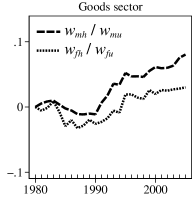
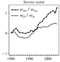
(b) Skilled vs. unskilled

Notes: The wages of male skilled, female skilled, male unskilled, and female unskilled labor are denoted by $w_{mh}$, $w_{fh}$, $w_{mu}$, and $w_{fu}$, respectively. All the series are logarithmically transformed and normalized to zero in the year 1980. The 1980 values of the skilled gender wage gap, $w_{mh}/w_{fh}$, unskilled gender wage gap, $w_{mu}/w_{fu}$, male skill wage gap, $w_{mh}/w_{mu}$, and female skill wage gap, $w_{fh}/w_{fu}$, are 1.42 (1.33), 1.50 (1.42), 1.70 (1.60), and 1.79 (1.69) in the goods (service) sector, respectively.

Figure 2: Gender and skill premia in the United States

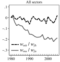
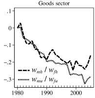
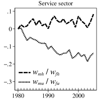
(a) Male vs. female

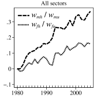
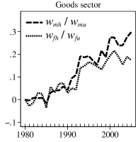
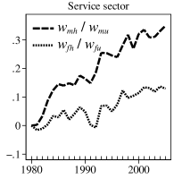
(b) Skilled vs. unskilled

Notes: The wages of male skilled, female skilled, male unskilled, and female unskilled labor are denoted by $w_{mh}$, $w_{fh}$, $w_{mu}$, and $w_{fu}$, respectively. All the series are logarithmically transformed and normalized to zero in the year 1980. The 1980 values of the skilled gender wage gap, $w_{mh}/w_{fh}$, unskilled gender wage gap, $w_{mu}/w_{fu}$, male skill wage gap, $w_{mh}/w_{mu}$, and female skill wage gap, $w_{fh}/w_{fu}$, are 1.62 (1.40), 1.58 (1.55), 1.57 (1.49), and 1.53 (1.66) in the goods (service) sector, respectively.

5.2 Trends

During the period between the years 1980 and 2005, there was a difference in the trends of the gender wage gap between skilled and unskilled workers in OECD countries (Figure 1a). The male–female wage gap declined among unskilled workers, but not among skilled workers. Looking at the trends separately for the goods and services sectors, the difference is evident in the services sector, but not in the goods sector. At the same time, there was a difference in the trends of the skill wage gap between male and female workers in OECD countries (Figure 1b). The skilled–unskilled wage gap increased among male workers after a slight drop in the early 1980s, while it did not increase among female workers except for the period between the years 1987 and 1995. Looking at the trends separately for the goods and services sectors, the difference is again evident in the services sector, but not in the goods sector. Taken together, the rate of decrease in the male–female wage gap was greater among unskilled workers than among skilled workers, while the rate of increase in the skilled–unskilled wage gap was greater among male workers than among female workers. This finding is perhaps surprising but not inconsistent with the fact that the rate of decline in the gender wage gap was greater at the middle or bottom than at the top of the wage distribution in the United States from the 1980s to the 2000s (Blau and Kahn, 2017). In fact, the pattern of changes in gender and skill premia mentioned above is clearer in the United States (Figures 2a and 2b).

Figure 3: Relative labor quantities

(a) Male vs. female

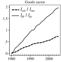
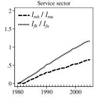
(b) Skilled vs. unskilled

Notes: The quantities of male skilled, female skilled, male unskilled, and female unskilled labor are denoted by $\ell_{mh}$, $\ell_{fh}$, $\ell_{mu}$, and $\ell_{fu}$, respectively. All the series are logarithmically transformed and normalized to zero in the year 1980. The 1980 values of the skilled male–female ratio, $\ell_{mh}/\ell_{fh}$, unskilled male–female ratio, $\ell_{mu}/\ell_{fu}$, male skilled–unskilled ratio, $\ell_{mh}/\ell_{mu}$, and female skilled–unskilled ratio, $\ell_{fh}/\ell_{fu}$, are 13.6 (3.88), 3.42 (1.27), 0.08 (0.21), and 0.03 (0.11) in the goods (service) sector, respectively.

Turning to the relative quantities of labor, there was a decline in the quantity of male labor relative to female labor, except for unskilled labor in the goods sector, and an increase in the quantity of skilled labor relative to unskilled labor. The rate of decline in the relative quantity of male labor was much greater for skilled labor than for unskilled labor (Figure 3a). At the same time, the rate of increase in the relative quantity of skilled labor was much greater for female labor than for male labor (Figure 3b). The differences are evident in both sectors but greater in the goods sector than in the services sector. Specifically, the rate of decline in the relative quantity of male skilled labor to female skilled labor was greater in the goods sector than in the services sector, while the rate of increase in the relative quantity of female skilled labor to female unskilled labor was greater in the goods sector than in the services sector. These observations suggest that we may need to take into account a sectoral difference in production technology to explain the sectoral differences in the trends of the gender wage gap and the skill wage gap.

The trends in the rental prices of capital differ significantly between ICT and non-ICT capital (Figure 4). The rental price of ICT capital fell dramatically, but that of non-ICT capital remained almost unchanged in both the goods and services sectors. Meanwhile, the quantities of both ICT and non-ICT capital increased in both sectors. However, the rate of increase in ICT capital was far greater than that in non-ICT capital in both sectors (Figure 5). Even if non-ICT equipment is distinguished from non-ICT structures, there is no significant difference in the trends of the prices and quantities between them (Figures A1 and A2 in Appendix A.3.3). These observations indicate substantial progress in ICT during the period.

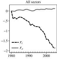
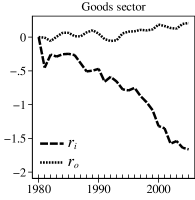
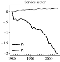
Figure 4: Rental prices of ICT and non-ICT capital

Notes: The rental prices of ICT and non-ICT capital are denoted by $r_{i}$ and $r_{o}$, respectively. All the series are logarithmically transformed and normalized to zero in the year 1980. The 1980 values of $r_{i}$ and $r_{o}$ are 0.97 (1.19) and 0.14 (0.07) in the goods (service) sector, respectively.

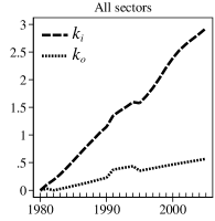
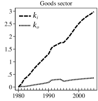
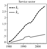
Figure 5: Quantities of ICT and non-ICT capital

Notes: The quantities of ICT and non-ICT capital are denoted by $k_{i}$ and $k_{o}$, respectively. All the series are logarithmically transformed and normalized to zero in the year 1980. The 1980 values of $k_{i}$ and $k_{o}$ are 4.95 (26.18) and 683.69 (1,874.42) billion U.S. dollars in the goods (service) sector, respectively.

The direction and magnitude of changes in labor shares vary by gender and skill in both the goods and services sectors (Figure 6). The income shares of male and female unskilled labor decreased, while the income shares of male and female skilled labor increased. The magnitude of the decline in the income share of male unskilled labor is significantly greater than that of the changes in the income shares of the other three types of labor. These observations indicate that the decline in the labor share is attributable to the decline in the income share of male unskilled labor.

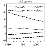
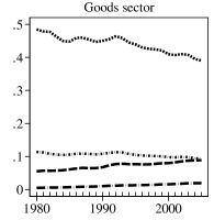
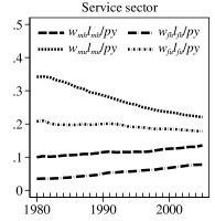
Figure 6: Income shares of the four types of labor

Notes: The income shares of male skilled labor, female skilled labor, male unskilled labor, and female unskilled labor are denoted by $w_{mh}\ell_{mh}/py$, $w_{fh}\ell_{fh}/py$, $w_{mu}\ell_{mu}/py$, and $w_{fu}\ell_{fu}/py$, respectively.

6 Results

We start this section by presenting the estimates of sectoral production function parameters and the contribution of specific factor inputs to sectoral changes in gender and skill premia. We then present the estimates of the aggregate elasticities of substitution and the contributions of specific factor inputs to aggregate changes in the relative wages and income shares of the four types of labor. We end this section by discussing the general equilibrium effects of technological change on the relative wages and income shares of the four types of labor.

6.1 Sectoral results

6.1.1 Production function

Table 1 reports the estimates of the substitution parameters in the production functions for the goods and services sectors. The estimates are presented separately for the cases in which the most relevant and full sets of moment conditions are used and separately for the cases in which 5- and 10-year differences are used. For all cases, significant differences are observed in the estimates of the four substitution parameters in both sectors. All the estimates are consistent with the capital–skill–gender complementarity hypothesis that ICT equipment is more complementary not only to skilled labor than unskilled labor but also to female labor than male labor (i.e., $\sigma_{fh}<\sigma_{mh}<\sigma_{fu}<\sigma_{mu}$). The null hypotheses of $\sigma_{fh}=\sigma_{mh}$, $\sigma_{mh}=\sigma_{fu}$, and $\sigma_{fu}=\sigma_{mu}$ are all rejected at the 1 percent significance level. The results imply that the male–female wage gap would decline with the expansion of ICT equipment, while the skilled–unskilled wage gap would increase with the expansion of ICT equipment.

Table 1: Production function estimates

	Goods sector					Services sector
	$\sigma_{fh}$	$\sigma_{mh}$	$\sigma_{fu}$	$\sigma_{mu}$		$\sigma_{fh}$	$\sigma_{mh}$	$\sigma_{fu}$	$\sigma_{mu}$
	Most relevant set of moment conditions					Most relevant set of moment conditions
5-yr diff.	–0.817	0.243	0.535	0.718		–0.379	0.341	0.611	0.833
	(0.330)	(0.121)	(0.068)	(0.103)		(0.147)	(0.076)	(0.042)	(0.063)
10-yr diff.	–0.880	0.298	0.579	0.764		–0.525	0.328	0.601	0.833
	(0.469)	(0.063)	(0.043)	(0.050)		(0.201)	(0.058)	(0.040)	(0.057)
	Full set of moment conditions					Full set of moment conditions
5-yr diff.	–0.706	0.265	0.579	0.713		–0.387	0.338	0.629	0.842
	(0.304)	(0.053)	(0.048)	(0.050)		(0.134)	(0.055)	(0.037)	(0.049)
10-yr diff.	–0.924	0.309	0.592	0.732		–0.503	0.367	0.614	0.875
	(0.399)	(0.033)	(0.044)	(0.036)		(0.177)	(0.034)	(0.036)	(0.043)

Notes: Standard errors in parentheses are clustered at the country level.

The estimates of the substitution parameters differ significantly between the goods and services sectors. The null hypothesis that the four substitution parameters are the same between the two sectors is rejected at the 1 percent significance level. In particular, ICT equipment is more complementary to female skilled labor in the goods sector than in the services sector.

The estimates are less susceptible to misspecification when the most relevant set of moment conditions is used. In this case, the over-identifying restrictions cannot be rejected with a Wald statistic of 0.000 (2.645) and a p-value of 0.983 (0.104) for the goods (service) sector when 5-year differences are used and with a Wald statistic of 0.404 (0.937) and a p-value of 0.525 (0.333) for the goods (service) sector when 10-year differences are used. We focus on the estimates obtained using the most relevant set of moment conditions in the subsequent analyses. The estimates are similar regardless of whether 5- or 10-year differences are used, but they are slightly more precise in the former case than in the latter case. We focus on the estimates obtained using 5-year differences in the subsequent analyses. When the most relevant set of moment conditions in 5-year differences are used, the first-stage F statistics of the hypothesis that the instruments are irrelevant for $\ell_{fh}/k_{i}$, $\tilde{D}/\ell_{mh}$, $\tilde{C}/\ell_{fu}$, and $\tilde{B}/\ell_{mu}$ are, respectively, 28.0 (59.4), 172.4 (92.3), 190.1 (76.7), and 85.7 (41.5) in the goods (service) sector.

6.1.2 Robustness checks

Table 2 shows the robustness of the results to controlling for the influence of labor market institutions, product market imperfections, and disembodied factor-biased technological change. The first three rows report the estimates of the substitution parameters after controlling for the influence of labor market institutions. We allow for the possibility that the actual wage may deviate from the competitive wage depending on the collective bargaining coverage, the strictness of employment protection legislation, and the presence and level of minimum wages. Specifically, we add the collective bargaining coverage and the employment protection legislation in log-difference form and the presence of minimum wages and its interaction with their level in first-difference form to equations (37)–(41). The relative magnitude of the estimated substitution parameters remains unchanged even though the standard errors become large due to the inclusion of irrelevant variables.

Table 2: Robustness checks

	Goods sector					Services sector
	$\sigma_{fh}$	$\sigma_{mh}$	$\sigma_{fu}$	$\sigma_{mu}$		$\sigma_{fh}$	$\sigma_{mh}$	$\sigma_{fu}$	$\sigma_{mu}$
Collective bargaining	–0.691	0.265	0.551	0.673		–0.418	0.239	0.665	0.880
coverage	(0.378)	(0.121)	(0.147)	(0.208)		(0.220)	(0.082)	(0.078)	(0.110)
Employment protection	–0.812	0.222	0.538	0.677		–0.520	0.231	0.620	0.865
legislation	(0.290)	(0.092)	(0.105)	(0.168)		(0.143)	(0.064)	(0.063)	(0.094)
Minimum wages	–0.586	0.318	0.586	0.771		–0.397	0.323	0.647	0.900
	(0.296)	(0.092)	(0.132)	(0.207)		(0.166)	(0.063)	(0.069)	(0.103)
Product market	–0.981	0.172	0.500	0.680		–0.550	0.232	0.544	0.774
imperfection	(0.330)	(0.129)	(0.068)	(0.110)		(0.186)	(0.086)	(0.043)	(0.060)
Disembodied factor-biased	–0.744	0.302	0.464	0.796		–0.239	0.395	0.573	0.887
technological change	(0.197)	(0.152)	(0.095)	(0.093)		(0.101)	(0.067)	(0.023)	(0.046)

Notes: Standard errors in parentheses are clustered at the country level.

The fourth row of Table 2 reports the estimates of the substitution parameters after taking into account imperfect competition in the product market. We can relax the assumption of competitive markets by recalculating the rental price of capital based on the external rate of return, because all the estimating equations hold regardless of the degree of markup. The estimates of the substitution parameters remain essentially unchanged.

The last row of Table 2 reports the estimates of the substitution parameters after controlling for disembodied factor-biased technological change. We take this into account by adding trend polynomials with country-specific coefficients in equations (37)–(41). Trend polynomials capture changes in the direction and magnitude of disembodied technological change, while country-specific coefficients capture cross-country differences in the speed and timing of disembodied technological change. We choose the order of the polynomials to fit the trends in relative wages for each sector and country. The estimates of the substitution parameters remain essentially unchanged. The results are robust to country-specific nonlinear time trends regardless of their causes even though the trends could be attributable in part to other unobserved factors such as discrimination and social norms.

6.1.3 Gender and skill premia in each sector

Table 3 presents the quantitative contributions of specific factor inputs to sectoral changes in gender and skill premia between the years 1980 and 2005. The first two columns report the actual and predicted changes in gender and skill premia. The gender wage gap tends to narrow, while the skill wage gap tends to widen. The rate of decline in the gender wage gap is greater for unskilled workers than for skilled workers, while the rate of increase in the skill wage gap is greater for male workers than for female workers. The differences are more significant in the services sector than in the goods sector. From these points of view, the observed pattern of sectoral changes in gender and skill premia is consistent with the pattern predicted from the model.

Table 3: Contributions to sectoral changes in gender and skill premia, 1980–2005

	Data		Model		$\Delta\ln k_{i}$		$\Delta\ln\ell_{fh}$		$\Delta\ln\ell_{mh}$		$\Delta\ln\ell_{fu}$		$\Delta\ln\ell_{mu}$		$\Delta\ln k_{o}$
	Goods sector
$\Delta\ln\left(\frac{w_{mh}}{w_{fh}}\right)$	–0.	066	–0.	156	–2.	229	2.	425	–0.	352	0.	000	0.	000	0.	000
			(0.	112)	(0.	241)	(0.	188)	(0.	029)	(0.	000)	(0.	000)	(0.	000)
$\Delta\ln\left(\frac{w_{mu}}{w_{fu}}\right)$	–0.	116	–0.	167	–0.	071	–0.	016	–0.	026	–0.	129	0.	075	0.	000
			(0.	022)	(0.	012)	(0.	003)	(0.	004)	(0.	013)	(0.	012)	(0.	000)
$\Delta\ln\left(\frac{w_{mh}}{w_{mu}}\right)$	0.	080	0.	023	0.	305	0.	069	–0.	242	–0.	033	–0.	075	0.	000
			(0.	027)	(0.	028)	(0.	006)	(0.	021)	(0.	006)	(0.	012)	(0.	000)
$\Delta\ln\left(\frac{w_{fh}}{w_{fu}}\right)$	0.	030	0.	012	2.	463	–2.	372	0.	084	–0.	162	0.	000	0.	000
			(0.	106)	(0.	247)	(0.	184)	(0.	012)	(0.	012)	(0.	000)	(0.	000)
	Services sector
$\Delta\ln\left(\frac{w_{mh}}{w_{fh}}\right)$	0.	018	–0.	027	–1.	026	1.	509	–0.	511	0.	000	0.	000	0.	000
			(0.	060)	(0.	105)	(0.	089)	(0.	036)	(0.	000)	(0.	000)	(0.	000)
$\Delta\ln\left(\frac{w_{mu}}{w_{fu}}\right)$	–0.	067	–0.	094	–0.	075	–0.	040	–0.	048	0.	088	–0.	019	0.	000
			(0.	015)	(0.	007)	(0.	004)	(0.	005)	(0.	008)	(0.	003)	(0.	000)
$\Delta\ln\left(\frac{w_{mh}}{w_{mu}}\right)$	0.	130	0.	110	0.	259	0.	139	–0.	343	0.	036	0.	019	0.	000
			(0.	022)	(0.	022)	(0.	012)	(0.	024)	(0.	003)	(0.	003)	(0.	000)
$\Delta\ln\left(\frac{w_{fh}}{w_{fu}}\right)$	0.	045	0.	044	1.	210	–1.	410	0.	120	0.	124	0.	000	0.	000
			(0.	051)	(0.	103)	(0.	083)	(0.	015)	(0.	008)	(0.	000)	(0.	000)

Notes: The first and second columns report the actual and predicted changes in the logarithms of relative wages. The predicted change is the sum of the contributions of each factor in the third to eighth columns. The contributions of each factor are computed using equations (29)–(32). Standard errors in parentheses are computed using bootstrap with 500 replications.

The third to eighth columns report the changes attributable to each factor input in the goods and services sectors. In both sectors, the skilled (unskilled) gender wage gap declines with the expansion of ICT equipment and increases with a rise in skilled (unskilled) female labor, while the male (female) skill wage gap increases with the expansion of ICT equipment and declines with a rise in male (female) skilled labor. Thus, whether the gender (skill) wage gap would eventually narrow (widen) depends on the relative magnitude of the capital–skill complementarity effect and the relative labor quantity effect. The magnitude of the capital–skill complementarity effects is greater in the goods sector than in the services sector, reflecting sectoral differences in the relative magnitude of the four substitution parameters. The direction and magnitude of the relative labor quantity effects differ between the goods and services sectors, reflecting sectoral differences in the direction and magnitude of changes in factor inputs as well as the magnitude of each substitution parameter. The relative labor quantity effects associated with a rise in female skilled labor are greater in the goods sector than in the services sector, while the relative labor quantity effects associated with a rise in male skilled labor are greater in the services sector than in the goods sector. The relative labor quantity effects associated with changes in male and female unskilled labor are negative in the goods sector but positive in the services sector. Overall, the relative magnitude of the capital–skill complementarity effect and the relative labor quantity effect accounts not only for the differences in changes in gender (skill) premia for skilled and unskilled (male and female) workers but also for the differences in changes in gender and skill premia for the goods and services sectors.

6.2 Aggregate results

6.2.1 Elasticities of substitution

Table 4 presents the estimates of the elasticities of substitution in the aggregate production and cost functions. The estimated elasticities of substitution between ICT equipment and the four types of labor are greater in the order of male unskilled, female unskilled, male skilled, and female skilled labor in terms of both the aggregate production and cost functions. The elasticity estimates imply that the expansion of ICT equipment would narrow the gender wage gap and widen the skill wage gap. Thus, the results are consistent with the literature that points to technological advances as causes of changes in the structure of wages and employment. The magnitude of the capital–skill complementarity effects is directly proportional to the differences in substitution elasticities as well as the rate of increase in ICT equipment. The elasticity estimates imply that the capital–skill complementarity effect on the gender (skill) wage gap would be greater for skilled (female) labor than for unskilled (male) labor. All else held constant, a 1 percent increase in ICT equipment would reduce the skilled (unskilled) gender wage gap by 0.32 (0.02) percent and raise the male (female) skill wage gap by 0.08 (0.38) percent. At the same time, the magnitude of the effects of labor quantities is inversely proportional to substitution elasticities and directly proportional to the rates of increases in the quantities of labor. The elasticity estimates imply that the effects of labor quantities would be greater in the order of female skilled, male skilled, female unskilled, and male unskilled labor.

Table 4: Aggregate elasticities of substitution

$\epsilon_{\ell_{f}\ell_{g}}^{\mathcal{F}}$														$\epsilon_{\ell_{f}\ell_{g}}^{\mathcal{C}}$
	$k_{i}$		$\ell_{fh}$		$\ell_{mh}$		$\ell_{fu}$		$\ell_{mu}$		$k_{o}$				$k_{i}$		$\ell_{fh}$		$\ell_{mh}$		$\ell_{fu}$		$\ell_{mu}$		$k_{o}$
$k_{i}$			0.	74	1.	46	2.	45	4.	88	1.	00		$k_{i}$			0.	76	1.	47	2.	48	4.	93	1.	00
			(0.	04)	(0.	10)	(0.	15)	(0.	75)	(0.	00)					(0.	05)	(0.	10)	(0.	15)	(0.	79)	(0.	00)
$\ell_{fh}$	0.	72			1.	50	2.	53	5.	07	1.	00		$\ell_{fh}$	0.	71			1.	48	2.	49	4.	96	1.	00
	(0.	04)			(0.	10)	(0.	16)	(0.	93)	(0.	00)			(0.	04)			(0.	10)	(0.	15)	(0.	80)	(0.	00)
$\ell_{mh}$	0.	94	1.	03			2.	47	4.	92	1.	00		$\ell_{mh}$	1.	06	1.	17			2.	47	4.	93	1.	00
	(0.	05)	(0.	06)			(0.	15)	(0.	77)	(0.	00)			(0.	06)	(0.	07)			(0.	15)	(0.	78)	(0.	00)
$\ell_{fu}$	0.	99	1.	10	1.	92			4.	94	1.	00		$\ell_{fu}$	1.	26	1.	40	2.	04			4.	93	1.	00
	(0.	06)	(0.	06)	(0.	11)			(0.	79)	(0.	00)			(0.	07)	(0.	08)	(0.	12)			(0.	79)	(0.	00)
$\ell_{mu}$	1.	01	1.	12	2.	17	3.	25			1.	00		$\ell_{mu}$	1.	52	1.	69	2.	77	3.	65			1.	00
	(0.	06)	(0.	07)	(0.	15)	(0.	26)			(0.	00)			(0.	12)	(0.	15)	(0.	30)	(0.	43)			(0.	00)
$k_{o}$	0.	97	1.	06	1.	72	1.	99	1.	68				$k_{o}$	1.	31	1.	45	2.	18	2.	69	3.	00
	(0.	05)	(0.	06)	(0.	08)	(0.	07)	(0.	04)					(0.	09)	(0.	10)	(0.	18)	(0.	24)	(0.	40)

Notes: The elasticities of substitution are computed using equations (12) and (13) and evaluated at the sample means across all countries and years. Standard errors in parentheses are computed using bootstrap with 500 replications.

The estimated elasticities of labor–labor substitution in the aggregate production (cost) function range from 1.0 to 5.1 (1.2 to 5.0). The elasticity estimates are within the range of standard estimates in the literature, although they are not strictly comparable to those in other studies because of differences in the degree of classification of labor. The estimated aggregate elasticities of substitution between female skilled labor and the other three types of labor are greater in the order of male unskilled, female unskilled, and male skilled labor. Both female skilled and unskilled labor are more complementary to male skilled labor than to male unskilled labor.

The Morishima (1967) elasticities of substitution are asymmetric by definition. The differences in the estimated elasticities of relative demand for capital with respect to wages are greater than those in the estimated elasticities of relative demand for labor with respect to the rental prices of capital. However, in both cases, ICT equipment is more complementary not only to skilled labor than unskilled labor but also to female labor than male labor.

The estimated elasticity of substitution between ICT equipment and male unskilled labor in the aggregate cost (production) function exceeds one at $\epsilon_{\ell_{mu}k_{i}}^{\mathcal{C}}=1.52$ ($\epsilon_{\ell_{mu}k_{i}}^{\mathcal{F}}=1.01$). ICT equipment is consistently more substitutable with male unskilled labor than with the other three types of labor both in terms of the aggregate production and cost functions. The results suggest that the income share of male unskilled labor is likely to decline with a fall in the price or a rise in the quantity of ICT equipment.

6.2.2 Gender and skill premia

Table 5 presents the quantitative contributions of specific factor inputs to aggregate changes in gender and skill premia. The first two columns report the actual and predicted changes in gender and skill premia. The rate of decline in the gender wage gap is greater for unskilled workers than for skilled workers, while the rate of increase in the skill wage gap is greater for male workers than for female workers. From this point of view, the observed pattern of aggregate changes in gender and skill premia is consistent with the pattern predicted from the model.

Table 5: Contributions to aggregate changes in gender and skill premia, 1980–2005

	Data		Model		FCE		RQE		$\Delta\ln k_{i}$		$\Delta\ln\ell_{fh}$		$\Delta\ln\ell_{mh}$		$\Delta\ln\ell_{fu}$		$\Delta\ln\ell_{mu}$		$\Delta\ln k_{o}$
$\Delta\ln\left(\frac{w_{mh}}{w_{fh}}\right)$	0.	018	0.	058	–0.	939	0.	997	–0.	939	1.	464	–0.	467	0.	002	0.	000	–0.	001
			(0.	056)	(0.	087)	(0.	059)	(0.	087)	(0.	083)	(0.	031)	(0.	001)	(0.	001)	(0.	000)
$\Delta\ln\left(\frac{w_{mu}}{w_{fu}}\right)$	–0.	056	–0.	077	–0.	140	0.	063	–0.	063	–0.	034	–0.	042	0.	049	0.	014	0.	000
			(0.	018)	(0.	015)	(0.	006)	(0.	007)	(0.	005)	(0.	005)	(0.	004)	(0.	002)	(0.	000)
$\Delta\ln\left(\frac{w_{mh}}{w_{mu}}\right)$	0.	090	0.	031	0.	368	–0.	337	0.	227	0.	125	–0.	323	0.	016	–0.	014	0.	000
			(0.	021)	(0.	027)	(0.	023)	(0.	017)	(0.	011)	(0.	022)	(0.	002)	(0.	002)	(0.	000)
$\Delta\ln\left(\frac{w_{fh}}{w_{fu}}\right)$	0.	016	–0.	104	1.	206	–1.	310	1.	104	–1.	373	0.	101	0.	063	0.	000	0.	001
			(0.	050)	(0.	089)	(0.	074)	(0.	087)	(0.	077)	(0.	014)	(0.	004)	(0.	001)	(0.	000)

Notes: The first and second columns report the actual and predicted changes in the logarithms of relative wages. The predicted change is the sum of the factor complementarity effect (FCE) and the relative quantity effect (RQE) in the third and fourth columns, or equivalently, the sum of the contributions of each factor in the fifth to tenth columns. The figures in the third to tenth columns are computed using equation (17). Standard errors in parentheses are computed using bootstrap with 500 replications.

The third and fourth columns report the changes attributable to the factor complementarity effect and the relative quantity effect. The fifth to tenth columns report the changes attributable to each factor input. This period shows a substantial increase in ICT capital and female skilled labor, a moderate increase in non-ICT capital and male skilled labor, a small increase in female unskilled labor, and a small decrease in male unskilled labor. The expansion of ICT equipment owing to technological progress contributes to narrowing the gender wage gap and widening the skill wage gap. Meanwhile, a rise in male and female skilled labor due to advances in educational attainment and female employment contributes to widening the gender wage gap and narrowing the skill wage gap. Consequently, whether the gender (skill) wage gap would narrow (widen) depends on the outcome of the race between progress in ICT and advances in female employment (educational attainment).

The factor complementarity effect associated with the expansion of ICT equipment is greater for the skilled gender wage gap and the female skill wage gap, reflecting the result that ICT equipment is significantly more complementary to female skilled labor than to the other three types of labor. If all else were held constant, the expansion of ICT equipment during the period would have reduced the skilled gender wage gap by 94 percent and raised the female skill wage gap by 110 percent. At the same time, the relative quantity effect is greater for the skilled gender wage gap and the female skill wage gap, reflecting the fact that the rate of increase in female skilled labor is significantly greater than that in the other three types of labor. If all else were held constant, a fall in the relative quantity of male skilled labor to female skilled labor during the period would have raised the skilled gender wage gap by 100 ($=(1.464-0.467)\times 100$) percent, and a rise in the relative quantity of female skilled labor to female unskilled labor would have reduced the female skill wage gap by 131 ($=(\text{\textendash}1.373+0.063)\times 100$) percent. Consequently, the skilled gender wage gap does not narrow as the two large effects cancel out. Similarly, the female skill wage gap does not widen as the two large effects cancel out. Meanwhile, the unskilled gender wage gap narrows as the factor complementarity effect exceeds the relative quantity effect. Similarly, the male skill wage gap widens as the factor complementarity effect exceeds the relative quantity effect. A rise in female skilled labor also increases the male skill wage gap as female skilled labor is more complementary to male skilled labor than to male unskilled labor. Given the results that the factor complementarity effects on the skilled gender wage gap and the female skill wage gap are so large, if there were no change in the relative supply of female skilled labor, the skilled gender wage gap would narrow more than the unskilled gender wage gap, and the female skill wage gap would widen more than the male skill wage gap. Taken together, a smaller rate of decline in the gender wage gap for skilled workers than for unskilled workers and a smaller rate of increase in the skill wage gap for female workers than for male workers are attributable not to a lack of demand for female skilled labor but to an abundance in the supply of female skilled labor.

6.2.3 Labor shares

Aggregate changes in the labor share can be decomposed into those in the income shares of the four types of labor $\ell_{f}$ for $f\in\mathscr{F}=\left\{mh,fh,mu,fu\right\}$, as shown in Corollary 4.

$$\Delta\ln\left(\frac{\sum_{f\in\mathscr{F}}\sum_{n}w_{fn}\ell_{fn}}{py}\right)=\sum_{f\in\mathscr{F}}\left(\frac{\sum_{n}w_{fn}\ell_{fn}}{\sum_{f\in\mathscr{F}}\sum_{n}w_{fn}\ell_{fn}}\right)\Delta\ln\left(\frac{\sum_{n}w_{fn}\ell_{fn}}{py}\right),$$ (49)

where $py=\sum_{f\in\mathscr{F}}\sum_{n}w_{fn}\ell_{fn}+\sum_{n}r_{in}k_{in}+\sum_{n}r_{on}k_{on}$. We evaluate the weights on the rates of changes in the income shares of each type of labor ($\sum_{n}w_{fn}\ell_{fn}/\sum_{f\in\mathscr{F}}\sum_{n}w_{fn}\ell_{fn}$) at the sample means across all countries and years. Aggregate changes in the labor share between the years 1980 and 2005 can be decomposed as

$$\Delta\ln\left(\frac{\sum_{f\in\mathscr{F}}\sum_{n}w_{fn}\ell_{fn}}{py}\right) = \underset{\textrm{male skilled}}{\underbrace{0.164\times 0.468}}+\underset{\textrm{female skilled}}{\underbrace{0.064\times 1.254}}+\underset{\textrm{male unskilled}}{\underbrace{0.515\times\left(-0.390\right)}}+\underset{\textrm{female unskilled}}{\underbrace{0.257\times\left(-0.107\right)}}$$

$$= 0.077+0.081-0.201-0.027.$$

This result indicates that the labor share did not decline uniformly across gender and skill groups. The income shares of male and female skilled labor increased, while the income shares of male and female unskilled labor declined. The reason for the decline in the labor share is that the majority of labor was unskilled to whom the share of income decreased. The decline in the labor share is attributable almost entirely to a fall in the income share of male unskilled labor.

Table 6: Contributions to aggregate changes in labor shares, 1980–2005

	Data		Model		FCE		RQE		$\Delta\ln k_{i}$		$\Delta\ln\ell_{fh}$		$\Delta\ln\ell_{mh}$		$\Delta\ln\ell_{fu}$		$\Delta\ln\ell_{mu}$		$\Delta\ln k_{o}$
$\Delta\ln\left(\frac{w_{mh}\ell_{mh}}{py}\right)$	0.	468	0.	459	0.	159	0.	300	0.	105	0.	050	0.	293	–0.	015	0.	026	0.	000
			(0.	017)	(0.	024)	(0.	013)	(0.	019)	(0.	012)	(0.	019)	(0.	001)	(0.	001)	(0.	000)
$\Delta\ln\left(\frac{w_{fh}\ell_{fh}}{py}\right)$	1.	254	1.	204	1.	095	0.	110	1.	044	0.	091	0.	059	–0.	017	0.	027	0.	001
			(0.	052)	(0.	085)	(0.	064)	(0.	090)	(0.	075)	(0.	014)	(0.	001)	(0.	001)	(0.	000)
$\Delta\ln\left(\frac{w_{mu}\ell_{mu}}{py}\right)$	–0.	390	–0.	340	–0.	248	–0.	091	–0.	123	–0.	074	–0.	085	–0.	031	–0.	027	0.	000
			(0.	012)	(0.	009)	(0.	012)	(0.	004)	(0.	003)	(0.	003)	(0.	001)	(0.	001)	(0.	000)
$\Delta\ln\left(\frac{w_{fu}\ell_{fu}}{py}\right)$	–0.	107	–0.	036	–0.	095	0.	059	–0.	060	–0.	040	–0.	042	0.	080	0.	026	0.	000
			(0.	011)	(0.	010)	(0.	008)	(0.	005)	(0.	004)	(0.	004)	(0.	003)	(0.	001)	(0.	000)

Notes: The first and second columns report the actual and predicted changes in the logarithms of labor shares. The predicted change is the sum of the factor complementarity effect (FCE) and the relative quantity effect (RQE) in the third and fourth columns, or equivalently, the sum of the contributions of each factor in the fifth to tenth columns. The figures in the third to tenth columns are computed using equation (15). Standard errors in parentheses are computed using bootstrap with 500 replications.

Table 6 presents the quantitative contributions of factor quantities to aggregate changes in the income shares of the four types of labor. The first two columns report the actual and predicted changes in the income shares of the four types of labor. The actual changes in the income shares of the four types of labor align with the changes predicted from the model. The predicted changes in the income shares of male and female skilled labor are positive and statistically significant, while those in the income shares of male and female unskilled labor are negative and statistically significant.

The third and fourth columns report the changes attributable to the factor complementarity effect and the relative quantity effect. The two effects work in the same direction for the income shares of male and female skilled labor and male unskilled labor. The former is much greater than the latter for the income shares of female skilled labor and male unskilled labor, although the converse is true for the income share of male skilled labor. The two effects work in the opposite direction for the income share of female unskilled labor. However, the direction of the factor complementarity effect aligns with that of the actual change for the income shares of all types of labor. Overall, the factor complementarity effect is essential for understanding changes in the income shares of multiple types of labor.

The fifth to tenth columns report the changes attributable to each factor input. The expansion of ICT equipment contributes significantly to the increase in the income shares of male and female skilled labor and the decrease in the income shares of male and female unskilled labor. The magnitude of the effect depends on the extent to which the rate of increase in the wages of male or female skilled (unskilled) labor is greater (smaller) than that in the nominal output. A rise in male and female skilled labor also contributes modestly to changes in labor shares.

6.2.4 Technological change

Table 7 presents the general equilibrium effects of three types of technological change on the relative wages and income shares of the four types of labor. The effects of technological change in Table 7 are measured in levels to facilitate interpretation of the magnitude of the effects on each relative wage and income share, whereas the contributions of factor inputs in Tables 3, 5, and 6 are measured in logarithms to facilitate comparison of the contributions to the four wage gaps or four income shares. The first to third columns report the changes attributable to technological change embodied in ICT equipment, technological change embodied in non-ICT equipment and structure, and sector-specific disembodied technological change, respectively, when labor is perfectly mobile across sectors. The effects of technological change embodied in ICT equipment are significant, whereas the effects of technological change embodied in non-ICT equipment and structure and of sector-specific disembodied technological change are marginal. The direction of the effects of technological change embodied in ICT equipment reflects the presence of capital–skill–gender complementarity and aligns with that of the effects of the expansion of ICT equipment in Tables 5 and 6. The results indicate that a fall in the relative price of ICT investment owing to technological progress contributes to a narrowing of the gender wage gap, a widening of the skill wage gap, an increase in the income share of skilled labor, and a decline in the income share of unskilled labor. The magnitude of the effect on labor shares is largest for male unskilled labor in percentage-point terms, while that of the effect on relative wages is largest for female skilled labor. The small effects of technological change embodied in non-ICT capital reflect the lack of significant decrease in the relative price of non-ICT investment and of complementarity among non-ICT capital, skills, and gender. The small effects of sector-specific disembodied technological change reflect the lack of significant change in sector-specific technology. The fourth to sixth columns report the changes attributable to the three types of technological change when labor is not perfectly mobile across sectors. The magnitude of the effects of technological change embodied in ICT equipment remains largely unchanged regardless of whether labor is perfectly mobile across sectors.

Table 7: General equilibrium effects of technological change, 1980–2005

	Perfect mobility							Imperfect mobility
	$\Delta\ln q_{i}$		$\Delta\ln q_{o}$		$\Delta\ln A_{n}$			$\Delta\ln q_{i}$		$\Delta\ln q_{o}$		$\Delta\ln A_{n}$
	Relative wages							Relative wages
$\Delta\left(\frac{w_{mh}}{w_{fh}}\right)$	–0.	855	–0.	010	0.	030		–0.	885	–0.	011	–0.	030
	(0.	055)	(0.	001)	(0.	006)		(0.	058)	(0.	001)	(0.	004)
$\Delta\left(\frac{w_{mu}}{w_{fu}}\right)$	–0.	061	–0.	001	–0.	010		–0.	034	–0.	001	–0.	122
	(0.	007)	(0.	000)	(0.	003)		(0.	007)	(0.	000)	(0.	001)
$\Delta\left(\frac{w_{mh}}{w_{mu}}\right)$	0.	262	0.	003	–0.	011		0.	226	0.	003	0.	116
	(0.	015)	(0.	000)	(0.	003)		(0.	015)	(0.	000)	(0.	001)
$\Delta\left(\frac{w_{fh}}{w_{fu}}\right)$	1.	331	0.	016	–0.	064		1.	366	0.	017	0.	009
	(0.	058)	(0.	001)	(0.	006)		(0.	063)	(0.	001)	(0.	004)
	Labor shares							Labor shares
$\Delta\left(\frac{w_{mh}\ell_{mh}}{py}\right)$	0.	006	0.	000	0.	000		0.	005	0.	000	0.	003
	(0.	001)	(0.	000)	(0.	000)		(0.	001)	(0.	000)	(0.	000)
$\Delta\left(\frac{w_{fh}\ell_{fh}}{py}\right)$	0.	015	0.	000	–0.	001		0.	016	0.	000	0.	001
	(0.	001)	(0.	000)	(0.	000)		(0.	001)	(0.	000)	(0.	000)
$\Delta\left(\frac{w_{mu}\ell_{mu}}{py}\right)$	–0.	034	0.	000	0.	001		–0.	030	0.	000	–0.	015
	(0.	003)	(0.	000)	(0.	001)		(0.	002)	(0.	000)	(0.	000)
$\Delta\left(\frac{w_{fu}\ell_{fu}}{py}\right)$	–0.	007	0.	000	0.	002		–0.	009	0.	000	0.	008
	(0.	001)	(0.	000)	(0.	000)		(0.	001)	(0.	000)	(0.	000)

Notes: The first to sixth columns report the changes attributable to technological change. The changes attributable to technological change in the first to third columns are computed using equations (19) and (20), while those in the fourth to sixth columns are computed using equations (23) and (24). Standard errors in parentheses are computed using bootstrap with 500 replications.

Table 8 presents the general equilibrium effects of technological change embodied in ICT equipment on the relative wages and income shares of the four types of labor for each value of the labor supply elasticity. For ease of reference, the first column reproduces the first column of Table 7, which corresponds to the case in which the labor supply elasticity is zero. Given the difficulty of selecting a single value of the aggregate hours elasticity (Chetty, Guren, Manoli and Weber, 2011; Keane and Rogerson, 2012), the second to fourth columns show how the effects vary according to the labor supply elasticity in the range of 0.5 to 2. The effects of technological change embodied in ICT equipment on the skilled gender wage gap and the female skill wage gap are greatest in absolute value when the supply of labor is exogenous and become smaller in absolute value as the supply of labor is more elastic. Progress in ICT raises the value of the marginal product of female skilled labor relative to other types of labor, and thus, the relative wages of female skilled labor. If the supply of labor is endogenous, the quantities of male (female) skilled labor relative to female skilled (unskilled) labor can decrease (increase) in response to progress in ICT. The decrease (increase) in the supply of male (female) skilled labor relative to female skilled (unskilled) labor moderates a fall (rise) in the skilled gender (female skill) wage gap. Such feedback effects become stronger as the supply of labor is more elastic. However, even if the labor supply elasticity is high at two, the effects of technological change embodied in ICT equipment on the skilled gender wage gap and the female skill wage gap remain greater than their observed changes. Moreover, the effects of technological change embodied in ICT equipment on the unskilled gender wage gap and the male skill wage gap do not vary substantially depending on the value of the labor supply elasticity. Even if the labor supply elasticity is high at two, the effect of technological change embodied in ICT equipment on the unskilled gender wage gap corresponds to 87 percent of its observed change, and that on the male skill wage gap is greater than its observed change. All else held constant, when the supply of labor is unit elastic, the fall in the relative price of ICT equipment would have reduced the skilled (unskilled) gender wage gap by 46 (7.5) percentage points and raised the male (female) skill wage gap by 26 (79) percentage points.

Table 8: General equilibrium effects of technological change embodied in ICT equipment, 1980–2005

$1/\gamma$	0		1/2		1		2
	Relative wages
$\Delta\left(\frac{w_{mh}}{w_{fh}}\right)$	–0.	855	–0.	603	–0.	464	–0.	317
	(0.	055)	(0.	044)	(0.	037)	(0.	028)
$\Delta\left(\frac{w_{mu}}{w_{fu}}\right)$	–0.	061	–0.	072	–0.	075	–0.	075
	(0.	007)	(0.	009)	(0.	010)	(0.	011)
$\Delta\left(\frac{w_{mh}}{w_{mu}}\right)$	0.	262	0.	270	0.	260	0.	231
	(0.	015)	(0.	014)	(0.	014)	(0.	015)
$\Delta\left(\frac{w_{fh}}{w_{fu}}\right)$	1.	331	0.	991	0.	792	0.	567
	(0.	058)	(0.	048)	(0.	042)	(0.	033)
	Labor shares
$\Delta\left(\frac{w_{mh}\ell_{mh}}{py}\right)$	0.	006	0.	010	0.	013	0.	018
	(0.	001)	(0.	001)	(0.	001)	(0.	001)
$\Delta\left(\frac{w_{fh}\ell_{fh}}{py}\right)$	0.	015	0.	017	0.	019	0.	020
	(0.	001)	(0.	001)	(0.	001)	(0.	001)
$\Delta\left(\frac{w_{mu}\ell_{mu}}{py}\right)$	–0.	034	–0.	048	–0.	060	–0.	078
	(0.	003)	(0.	004)	(0.	005)	(0.	007)
$\Delta\left(\frac{w_{fu}\ell_{fu}}{py}\right)$	–0.	007	–0.	008	–0.	007	–0.	006
	(0.	001)	(0.	001)	(0.	001)	(0.	002)

Notes: The changes in the levels of relative wages and labor shares attributable to technological change are computed using equations (21) and (22) for each value of the labor supply elasticity $1/\gamma$. Standard errors in parentheses are computed using bootstrap with 500 replications.

The effects of technological change embodied in ICT equipment on the income shares of the four types of labor tend to be smallest in absolute value when the supply of labor is exogenous and become greater in absolute value as the supply of labor is more elastic. Basically, the equilibrium wages increase less, but the equilibrium quantities increase more, as the labor supply elasticity increases. The effects of progress in ICT on labor shares become greater (smaller) as the labor supply elasticity increases if the rate of decrease in the equilibrium wages is small (large) relative to that of increase in the equilibrium quantities. The effects on the income shares of male and female skilled labor increase due to a greater increase in the equilibrium quantities, whereas the effect on the income shares of male unskilled labor decrease due to a greater decrease in the equilibrium quantities. The effect on the income share of female unskilled labor is insensitive to the value of the labor supply elasticity. All else held constant, the fall in the relative price of ICT equipment would have raised the income share of male (female) skilled labor by 1.3 (1.9) percentage points and reduced the income share of male (female) unskilled labor by 6.0 (0.7) percentage points in the case in which the supply of labor is unit elastic. In this case, the fall in the relative price of ICT equipment accounts for 33 (49) percent of the increase in the income share of male (female) skilled labor and 47 (43) percent of the decline in the income share of male (female) unskilled labor.

Table 6.2.4 presents the general equilibrium effects of technological change embodied in ICT equipment on the relative wages and income shares of the four types of labor by country for the cases in which the supply of labor is perfectly inelastic and unit elastic. For ease of reference, the first column reproduces the first and third columns of Table 8. The second to last columns report the effects evaluated at the sample means over time for each country. The results indicate that progress in ICT narrows the gender wage gap and widens the skill wage gap for all countries, while it increases the income share of skilled labor and decreases the income share of unskilled labor. The magnitude of the effects of progress in ICT varies across countries, depending on the rate of decrease in the relative price of ICT investment, as seen in the bottom row of Table 6.2.4, and on the income share of ICT equipment relative to the income shares of other factors, as described in Appendix A.2.5.

[ph] General equilibrium effects of technological change embodied in ICT equipment for each country

	All		AUS		AUT		CZE		DEU		DNK		FIN		GBR		ITA		JPN		NLD		USA
	Relative wages, $1/\gamma=0$
$\Delta\left(\frac{w_{mh}}{w_{fh}}\right)$	–0.	855	–1.	418	–0.	557	–0.	770	–0.	850	–3.	185	–0.	252	–0.	889	–0.	526	–1.	289	–1.	237	–0.	750
	(0.	055)	(0.	092)	(0.	036)	(0.	051)	(0.	056)	(0.	250)	(0.	013)	(0.	059)	(0.	037)	(0.	103)	(0.	096)	(0.	046)
$\Delta\left(\frac{w_{mu}}{w_{fu}}\right)$	–0.	061	–0.	135	–0.	032	–0.	054	–0.	047	–0.	174	–0.	019	–0.	073	–0.	037	–0.	069	–0.	069	–0.	069
	(0.	007)	(0.	018)	(0.	004)	(0.	007)	(0.	005)	(0.	019)	(0.	002)	(0.	008)	(0.	005)	(0.	008)	(0.	008)	(0.	008)
$\Delta\left(\frac{w_{mh}}{w_{mu}}\right)$	0.	262	0.	417	0.	234	0.	316	0.	227	1.	261	0.	089	0.	234	0.	229	0.	189	0.	443	0.	178
	(0.	015)	(0.	024)	(0.	015)	(0.	017)	(0.	013)	(0.	087)	(0.	004)	(0.	013)	(0.	017)	(0.	009)	(0.	025)	(0.	009)
$\Delta\left(\frac{w_{fh}}{w_{fu}}\right)$	1.	331	1.	854	1.	101	1.	431	1.	275	5.	439	0.	307	1.	454	0.	904	1.	898	2.	236	0.	925
	(0.	058)	(0.	078)	(0.	045)	(0.	065)	(0.	060)	(0.	287)	(0.	010)	(0.	068)	(0.	035)	(0.	129)	(0.	128)	(0.	039)
	Relative wages, $1/\gamma=1$
$\Delta\left(\frac{w_{mh}}{w_{fh}}\right)$	–0.	464	–0.	762	–0.	309	–0.	409	–0.	449	–1.	522	–0.	147	–0.	474	–0.	285	–0.	627	–0.	623	–0.	417
	(0.	037)	(0.	062)	(0.	025)	(0.	034)	(0.	036)	(0.	139)	(0.	010)	(0.	039)	(0.	025)	(0.	057)	(0.	057)	(0.	033)
$\Delta\left(\frac{w_{mu}}{w_{fu}}\right)$	–0.	075	–0.	160	–0.	040	–0.	064	–0.	057	–0.	191	–0.	023	–0.	089	–0.	042	–0.	078	–0.	080	–0.	086
	(0.	010)	(0.	022)	(0.	005)	(0.	009)	(0.	008)	(0.	025)	(0.	004)	(0.	012)	(0.	006)	(0.	011)	(0.	010)	(0.	011)
$\Delta\left(\frac{w_{mh}}{w_{mu}}\right)$	0.	260	0.	408	0.	225	0.	298	0.	212	1.	058	0.	089	0.	223	0.	203	0.	170	0.	399	0.	180
	(0.	014)	(0.	022)	(0.	013)	(0.	017)	(0.	012)	(0.	070)	(0.	005)	(0.	012)	(0.	013)	(0.	010)	(0.	022)	(0.	010)
$\Delta\left(\frac{w_{fh}}{w_{fu}}\right)$	0.	792	1.	102	0.	669	0.	832	0.	731	2.	903	0.	195	0.	843	0.	548	0.	972	1.	221	0.	557
	(0.	042)	(0.	055)	(0.	034)	(0.	045)	(0.	041)	(0.	167)	(0.	008)	(0.	047)	(0.	026)	(0.	071)	(0.	077)	(0.	029)
	Labor shares, $1/\gamma=0$
$\Delta\left(\frac{w_{mh}\ell_{mh}}{py}\right)$	0.	006	0.	007	0.	004	0.	005	0.	005	0.	016	0.	001	0.	004	0.	004	0.	005	0.	009	0.	003
	(0.	001)	(0.	001)	(0.	001)	(0.	001)	(0.	001)	(0.	002)	(0.	000)	(0.	001)	(0.	000)	(0.	001)	(0.	001)	(0.	001)
$\Delta\left(\frac{w_{fh}\ell_{fh}}{py}\right)$	0.	015	0.	015	0.	015	0.	022	0.	015	0.	022	0.	011	0.	007	0.	009	0.	006	0.	006	0.	020
	(0.	001)	(0.	001)	(0.	001)	(0.	001)	(0.	001)	(0.	001)	(0.	000)	(0.	000)	(0.	000)	(0.	000)	(0.	000)	(0.	001)
$\Delta\left(\frac{w_{mu}\ell_{mu}}{py}\right)$	–0.	034	–0.	064	–0.	022	–0.	024	–0.	023	–0.	103	–0.	011	–0.	033	–0.	027	–0.	029	–0.	045	–0.	032
	(0.	003)	(0.	006)	(0.	002)	(0.	002)	(0.	002)	(0.	008)	(0.	001)	(0.	003)	(0.	002)	(0.	002)	(0.	004)	(0.	003)
$\Delta\left(\frac{w_{fu}\ell_{fu}}{py}\right)$	–0.	007	–0.	008	–0.	006	–0.	007	–0.	005	–0.	029	–0.	004	–0.	006	–0.	005	–0.	004	–0.	004	–0.	007
	(0.	001)	(0.	001)	(0.	001)	(0.	001)	(0.	001)	(0.	004)	(0.	000)	(0.	001)	(0.	001)	(0.	001)	(0.	001)	(0.	001)
	Labor shares, $1/\gamma=1$
$\Delta\left(\frac{w_{mh}\ell_{mh}}{py}\right)$	0.	013	0.	015	0.	009	0.	011	0.	011	0.	028	0.	004	0.	009	0.	007	0.	012	0.	017	0.	010
	(0.	001)	(0.	001)	(0.	001)	(0.	001)	(0.	001)	(0.	003)	(0.	001)	(0.	001)	(0.	001)	(0.	001)	(0.	001)	(0.	002)
$\Delta\left(\frac{w_{fh}\ell_{fh}}{py}\right)$	0.	019	0.	018	0.	018	0.	025	0.	017	0.	023	0.	014	0.	008	0.	011	0.	007	0.	007	0.	023
	(0.	001)	(0.	001)	(0.	001)	(0.	002)	(0.	001)	(0.	001)	(0.	001)	(0.	000)	(0.	001)	(0.	001)	(0.	000)	(0.	001)
$\Delta\left(\frac{w_{mu}\ell_{mu}}{py}\right)$	–0.	060	–0.	111	–0.	039	–0.	041	–0.	038	–0.	158	–0.	020	–0.	056	–0.	045	–0.	045	–0.	072	–0.	056
	(0.	005)	(0.	009)	(0.	003)	(0.	004)	(0.	003)	(0.	014)	(0.	002)	(0.	005)	(0.	004)	(0.	004)	(0.	006)	(0.	004)
$\Delta\left(\frac{w_{fu}\ell_{fu}}{py}\right)$	–0.	007	–0.	007	–0.	006	–0.	008	–0.	005	–0.	025	–0.	006	–0.	005	–0.	003	–0.	004	–0.	001	–0.	009
	(0.	001)	(0.	002)	(0.	001)	(0.	001)	(0.	001)	(0.	005)	(0.	001)	(0.	001)	(0.	001)	(0.	001)	(0.	001)	(0.	001)
	Progress in ICT
$\Delta\ln q_{i}$	1.	972	2.	518	1.	978	1.	316	1.	374	3.	323	1.	296	1.	571	1.	713	1.	376	1.	797	1.	923

Notes: Country names are abbreviated as follows: AUS, Australia; AUT, Austria; CZE, the Czech Republic; DEU, Germany; DNK, Denmark; FIN, Finland; GBR, the United Kingdom; ITA, Italy; JPN, Japan; NLD, the Netherlands; and USA, the United States. The changes in the levels of relative wages and labor shares attributable to technological change are computed using equations (21) and (22) for each value of the labor supply elasticity $1/\gamma$. Standard errors in parentheses are computed using bootstrap with 500 replications.

7 Conclusion

We developed a unified framework to measure the contributions of specific factor inputs to aggregate changes in the relative wages and income shares of different types of labor and to quantify the general equilibrium effects of capital-embodied technological change on the relative wages and income shares of different types of labor. We applied this framework to developed economies consisting of multiple sectors, where two types of capital (ICT and non-ICT capital) and four types of labor (male skilled, female skilled, male unskilled, and female unskilled labor) are used to produce goods and services.

Our results show that the expansion of ICT equipment owing to technological progress results in an increase in the skill wage gap and a decline in the gender wage gap, while the increased supply of male and female skilled labor due to advances in educational attainment and female employment prevents an increase in the skill wage gap and a decline in the gender wage gap. The observed patterns of sectoral and aggregate changes in the four wage gaps (skilled gender wage gap, unskilled gender wage gap, male skill wage gap, and female skill wage gap) can be explained in terms of the race between progress in ICT and advances in educational attainment and female employment. The unskilled gender wage gap is more likely to decline than the skilled gender wage gap, while the male skill wage gap is more likely to increase than the female skill wage gap. The reason for this is not because the demand for female skilled labor is insufficient but because the supply of female skilled labor becomes abundant. Our results further show that the general equilibrium effects of technological change embodied in ICT equipment are sufficiently large to account for the narrowing of the unskilled gender wage gap, the widening of the male skill wage gap, and about half of the decline in the income share of male unskilled labor, which accounts for most of the decline in the labor share.

Our findings have implications for policies aimed at promoting female employment, technological progress, and educational attainment. The role of these policies is similar in that they could help raise national income but different in that they could widen or narrow the gender wage gap and the skill wage gap. The male–female wage gap would decrease as a result of policies that raise the relative demand for female labor (e.g., tax credits for and grant funding to research and development), whereas it would increase as a result of policies that raise the relative supply of female labor (e.g., maternity leave, childcare facilities, and the equal employment opportunity law). At the same time, the skilled–unskilled wage gap would decrease as a result of policies that raise the relative supply of skilled labor (e.g., tuition exemption and subsidies), whereas it would increase as a result of policies that raise the relative demand for skilled labor (e.g., tax credits for and grant funding to research and development). Our findings suggest not only that policies promoting educational attainment would be effective in reducing the skill wage gap but also that policies promoting technological progress would be effective in reducing the gender wage gap.

Appendix A Appendix

A.1 Proofs of propositions

Proof of Proposition 1

Using the facts that $\partial\ln\mathcal{F}(\ell_{1},...,\ell_{F})/\partial\ln\ell_{f}=\Lambda_{\ell_{f}}$ and $\partial\ln\mathcal{C}(w_{1},...,w_{F},y)/\partial\ln w_{f}=\Lambda_{\ell_{f}}$, the aggregate elasticities of substitution can be rewritten as

$$\frac{1}{\epsilon_{\ell_{f}\ell_{g}}^{\mathcal{F}}}= \frac{\partial\ln\Lambda_{\ell_{f}}}{\partial\ln\ell_{g}}-\frac{\partial\ln\Lambda_{\ell_{g}}}{\partial\ln\ell_{g}}+1,$$ (A1)

$$\epsilon_{\ell_{f}\ell_{g}}^{\mathcal{C}}= \frac{\partial\ln\Lambda_{\ell_{f}}}{\partial\ln w_{g}}-\frac{\partial\ln\Lambda_{g}}{\partial\ln w_{g}}+1.$$ (A2)

The first-order Taylor expansion of the factor share, $\Lambda_{\ell_{f}}=\sum_{n=1}^{N}\zeta_{n}\lambda_{\ell_{f}n}$, yields

$$\Delta\ln\Lambda_{\ell_{f}}=\sum_{n=1}^{N}\frac{\zeta_{n}\lambda_{\ell_{f}n}}{\Lambda_{\ell_{f}}}\Delta\ln\zeta_{n}+\sum_{n=1}^{N}\frac{\zeta_{n}\lambda_{\ell_{f}n}}{\Lambda_{\ell_{f}}}\Delta\ln\lambda_{\ell_{f}n}.$$ (A3)

The first-order Taylor expansion of the factor share in sector $n$, $\lambda_{\ell_{f}n}=w_{f}\ell_{fn}/p_{n}y_{n}$, yields

$$\Delta\ln\lambda_{\ell_{f}n}=\sum_{g=1}^{F}\frac{\partial\ln\lambda_{\ell_{f}n}}{\partial\ln w_{g}}\Delta\ln w_{g}.$$ (A4)

The first-order Taylor expansion of the expenditure share (6) yields

$$\Delta\ln\zeta_{n}=-\frac{\eta}{1-\eta}\Delta\ln p_{n}+\frac{\eta}{1-\eta}\sum_{m=1}^{N}\zeta_{m}\Delta\ln p_{m}.$$ (A5)

The first-order Taylor expansion of the profit maximizing condition, $p_{n}=\mathcal{\mathcal{\widetilde{C}}}_{n}(w_{1},\ldots,w_{F})/A_{n}$, yields

$$\Delta\ln p_{n}=\sum_{f=1}^{F}\lambda_{\ell_{f}n}\Delta\ln w_{f}-\Delta\ln A_{n}.$$ (A6)

Substituting this into equation (A5) yields

$$\Delta\ln\zeta_{n}=\left(1-\frac{1}{1-\eta}\right)\left[\sum_{f=1}^{F}\left(\lambda_{\ell_{f}n}-\Lambda_{\ell_{f}}\right)\Delta\ln w_{f}-\Delta\ln A_{n}+\sum_{m=1}^{N}\zeta_{m}\Delta\ln A_{m}\right].$$ (A7)

Substituting equations (A4) and (A7) into equation (A3) yields

$$\Delta\ln\Lambda_{\ell_{f}}=\sum_{g=1}^{F}\Psi_{\left(f,g\right)}^{w}\Delta\ln w_{g}+\psi_{\left(f\right)}^{w}=\sum_{g=1}^{F}\Psi_{\left(f,g\right)}^{w}\Delta\ln\left(\frac{w_{g}}{p}\right)+\psi_{\left(f\right)}^{w}.$$ (A8)

The second equality comes from the fact that equation (A8) is homogeneous of degree zero in factor prices because $\sum_{g=1}^{F}\Psi_{\left(f,g\right)}^{w}=0$. By the definition of factor shares, $\Delta\ln w_{f}=\Delta\ln\Lambda_{\ell_{f}}-\Delta\ln\ell_{f}+\Delta\ln(py)$. Substituting this into equation (A8) yields

$$\Delta\ln\Lambda_{\ell_{f}}=\sum_{g=1}^{F}\Psi_{\left(f,g\right)}^{w}\Delta\ln\Lambda_{\ell_{g}}-\sum_{g=1}^{F}\Psi_{\left(f,g\right)}^{w}\Delta\ln\ell_{g}+\psi_{\left(f\right)}^{w}.$$

Solving the system of equations for $\Delta\ln\Lambda_{\ell_{f}}$ yields

$$\Delta\ln\Lambda_{\ell_{f}}=\sum_{g=1}^{F}\Psi_{\left(f,g\right)}^{\ell}\Delta\ln\ell_{g}+\psi_{\left(f\right)}^{\ell}.$$ (A9)

Equation (A9) implies $\partial\ln\Lambda_{\ell_{f}}/\partial\ln\ell_{g}=\Psi_{\left(f,g\right)}^{\ell}$, while equation (A8) implies $\partial\ln\Lambda_{\ell_{f}}/\partial\ln w_{g}=\Psi_{\left(f,g\right)}^{w}$. Substituting these into equations (A1) and (A2) yields equations (12) and (13).

Proof of Proposition 2

Using the fact that $\sum_{f=1}^{F}\Lambda_{\ell_{f}}\Psi_{\left(f,g\right)}^{\ell}=0$, equation (A9) can be rearranged as

$$\Delta\ln\Lambda_{\ell_{f}}=\sum_{g\neq f}^{F}\left[1-\left(\Psi_{\left(g,f\right)}^{\ell}-\Psi_{\left(f,f\right)}^{\ell}+1\right)\right]\Lambda_{\ell_{g}}\Delta\ln\ell_{f}+\sum_{g\neq f}^{F}\left[\left(\Psi_{\left(f,g\right)}^{\ell}-\Psi_{\left(g,g\right)}^{\ell}+1\right)-1\right]\Lambda_{\ell_{g}}\Delta\ln\ell_{g}\\ +\sum_{g\neq f}^{F}\sum_{h\neq f,g}^{F}\left[\left(\Psi_{\left(f,g\right)}^{\ell}-\Psi_{\left(g,g\right)}^{\ell}+1\right)-\left(\Psi_{\left(h,g\right)}^{\ell}-\Psi_{\left(g,g\right)}^{\ell}+1\right)\right]\Lambda_{\ell_{h}}\Delta\ln\ell_{g}+\psi_{\left(f\right)}^{\ell}.$$

Substituting equation (12) into this yields equation (15).

Similarly, using the fact that $\sum_{f=1}^{F}\Lambda_{\ell_{f}}\Psi_{\left(f,g\right)}^{w}=0$, equation (A8) can be rearranged as

$$\Delta\ln\Lambda_{\ell_{f}}=\sum_{g\neq f}^{F}\left[1-\left(\Psi_{\left(g,f\right)}^{w}-\Psi_{\left(f,f\right)}^{w}+1\right)\right]\Lambda_{\ell_{g}}\Delta\ln w_{f}+\sum_{g\neq f}^{F}\left[\left(\Psi_{\left(f,g\right)}^{w}-\Psi_{\left(g,g\right)}^{w}+1\right)-1\right]\Lambda_{\ell_{g}}\Delta\ln w_{g}\\ +\sum_{g\neq f}^{F}\sum_{h\neq f,g}^{F}\left[\left(\Psi_{\left(f,g\right)}^{w}-\Psi_{\left(g,g\right)}^{w}+1\right)-\left(\Psi_{\left(h,g\right)}^{w}-\Psi_{\left(g,g\right)}^{w}+1\right)\right]\Lambda_{\ell_{h}}\Delta\ln w_{g}+\psi_{\left(f\right)}^{w}.$$

Substituting equation (13) into this yields equation (16).

Proof of Proposition 3

By definition, the log change of relative factor shares can be written as

$$\Delta\ln\left(\frac{\Lambda_{\ell_{f}}}{\Lambda_{\ell_{g}}}\right)=\Delta\ln\left(\frac{w_{f}}{w_{g}}\right)+\Delta\ln\left(\frac{\ell_{f}}{\ell_{g}}\right).$$ (A10)

Substituting equation (A9) into equation (A10) yields

$$\Delta\ln\left(\frac{w_{f}}{w_{g}}\right)=\sum_{h=1}^{F}\left[\Psi_{\left(f,h\right)}^{\ell}-\Psi_{\left(h,h\right)}^{\ell}+1-\left(\Psi_{\left(g,h\right)}^{\ell}-\Psi_{\left(h,h\right)}^{\ell}+1\right)\right]\Delta\ln\ell_{h}-\Delta\ln\ell_{f}+\Delta\ln\ell_{g}+\psi_{\left(f\right)}^{\ell}-\psi_{\left(g\right)}^{\ell}.$$

Using equation (12), this equation can be rewritten as equation (17).

Substituting (A8) into equation (A10) yields

$$\Delta\ln\left(\frac{\ell_{f}}{\ell_{g}}\right)=\sum_{h=1}^{F}\left[\Psi_{\left(f,h\right)}^{w}-\Psi_{\left(h,h\right)}^{w}+1-\left(\Psi_{\left(g,h\right)}^{w}-\Psi_{\left(h,h\right)}^{w}+1\right)\right]\Delta\ln w_{h}-\Delta\ln w_{f}+\Delta\ln w_{g}+\psi_{\left(f\right)}^{w}-\psi_{\left(g\right)}^{w}.$$

Using equation (13), this equation can be rewritten as equation (18).

Proof of Proposition 4

The Euler equation (A59) can be derived from the household’s problem when the interest rate is defined as $\iota_{t}=(1/\beta)[(\partial\mathcal{U}(c_{t-1})/\partial c_{t-1})/(\partial\mathcal{U}(c_{t})/\partial c_{t})]-1$. It follows that the log change in the rental price of capital between steady states are given by

$$d\ln\left(\frac{r_{f}}{p}\right)=-d\ln q_{f}.$$ (A11)

Subtracting $d\ln p$ from both sides of equation (A6) and substituting equation (A11) into this yields

$$d\ln\left(\frac{p_{n}}{p}\right)=\sum_{f=1}^{F_{\ell}}\lambda_{\ell_{f}n}d\ln\left(\frac{w_{f}}{p}\right)-\sum_{f=1}^{F_{k}}\lambda_{k_{f}n}d\ln q_{f}-d\ln A_{n}.$$ (A12)

The first-order Taylor expansion of the aggregate price, $p=(\sum_{n=1}^{N}\theta_{cn}^{1/(1-\eta)}p_{n}^{-\eta/(1-\eta)})^{-(1-\eta)/\eta}$, yields $\sum_{n=1}^{N}\zeta_{n}d\ln(p_{n}/p)=0$. Substituting equation (A12) into this yields

$$\sum_{f=1}^{F_{\ell}}\Lambda_{\ell_{f}}d\ln\left(\frac{w_{f}}{p}\right)=\sum_{f=1}^{F_{k}}\Lambda_{k_{f}}d\ln q_{f}+\sum_{n=1}^{N}\zeta_{n}d\ln A_{n}.$$ (A13)

Equation (A8) can be rewritten as

$$d\ln\Lambda_{\ell_{f}}=\sum_{g=1}^{F}\Psi_{\left(f,g\right)}^{w}d\ln\left(\frac{w_{g}}{p}\right)+\sum_{n=1}^{N}\Phi_{\left(f,n\right)}^{w}d\ln A_{n},$$

where $\Phi^{w}$ is the $F\times N$ matrix whose $fn$-th element is given by $\Phi_{\left(f,n\right)}^{w}=-[1-1/(1-\eta)](\zeta_{n}\lambda_{\ell_{f}n}/\Lambda_{\ell_{f}}-\zeta_{n})$. Let the matrix $\Psi^{w}$ be partitioned as

$$\Psi^{w}=\left[\begin{array}[]{cc}\Psi_{UL}^{w}&\Psi_{UR}^{w}\\ \Psi_{LL}^{w}&\Psi_{LR}^{w}\end{array}\right],$$

where $\Psi_{UL}^{w}$, $\Psi_{UR}^{w}$, $\Psi_{LL}^{w}$, and $\Psi_{LR}^{w}$ are $F_{\ell}\times F_{\ell}$, $F_{\ell}\times F_{k}$, $F_{k}\times F_{\ell}$, and $F_{k}\times F_{k}$ matrices, respectively. The equation can be further rewritten as

$$d\ln\Lambda_{\ell_{f}}=\sum_{g=1}^{F_{\ell}}\Psi_{UL\left(f,g\right)}^{w}d\ln\left(\frac{w_{g}}{p}\right)+\sum_{g=1}^{F_{k}}\Psi_{UR\left(f,g\right)}^{w}d\ln\left(\frac{r_{g}}{p}\right)+\sum_{n=1}^{N}\Phi_{\left(f,n\right)}^{w}d\ln A_{n}\quad\text{for }f=1,\ldots,F_{\ell}.$$

Substituting equation (A11) into this yields

$$d\ln\Lambda_{\ell_{f}}=\sum_{g=1}^{F_{\ell}}\Psi_{UL\left(f,g\right)}^{w}d\ln\left(\frac{w_{g}}{p}\right)-\sum_{g=1}^{F_{k}}\Psi_{UR\left(f,g\right)}^{w}d\ln q_{g}+\sum_{n=1}^{N}\Phi_{\left(f,n\right)}^{w}d\ln A_{n}\quad\text{for }f=1,\ldots,F_{\ell}.$$ (A14)

Substituting $\Lambda_{\ell_{f}}=w_{f}\ell_{f}/py$ into this yields

$$\sum_{g=1}^{F_{\ell}}\left(\Psi_{UL\left(f,g\right)}^{w}-I_{\left(f,g\right)}\right)d\ln\left(\frac{w_{g}}{p}\right)=\sum_{g=1}^{F_{\ell}}I_{\left(f,g\right)}d\ln\ell_{g}\\ +\sum_{g=1}^{F_{k}}\Psi_{UR\left(f,g\right)}^{w}d\ln q_{g}-\sum_{n=1}^{N}\Phi_{\left(f,n\right)}^{w}d\ln A_{n}-d\ln y\quad\text{for }f=1,\ldots,F_{\ell}.$$ (A15)

Subtracting the equation for $f=F_{\ell}$ from that for any $f\in\{1,\ldots,F_{\ell}-1$} yields

$$\sum_{g=1}^{F_{\ell}}\left(\Psi_{UL\left(f,g\right)}^{w}-\Psi_{UL\left(F_{\ell},g\right)}^{w}-I_{\left(f,g\right)}+I_{\left(F_{\ell},g\right)}\right)d\ln\left(\frac{w_{g}}{p}\right)=\sum_{g=1}^{F_{\ell}}\left(I_{\left(f,g\right)}-I_{\left(F_{\ell},g\right)}\right)d\ln\ell_{g}\\ +\sum_{g=1}^{F_{k}}\left(\Psi_{UR\left(f,g\right)}^{w}-\Psi_{UR\left(F_{\ell},g\right)}^{w}\right)d\ln q_{g}-\sum_{n=1}^{N}\left(\Phi_{\left(f,n\right)}^{w}-\Phi_{\left(F_{\ell},n\right)}^{w}\right)d\ln A_{n}.$$ (A16)

Solving the system of equations (A13) and (A16) for $d\ln(w_{f}/p)$ and setting $d\ln\ell_{f}=0$ yields

$$d\ln\left(\frac{w_{f}}{p}\right)=\sum_{g=1}^{F_{k}}\Upsilon_{\left(f,g\right)}^{q}d\ln q_{g}+\sum_{n=1}^{N}\Upsilon_{\left(f,n\right)}^{A}d\ln A_{n}\quad\text{for }f=1,\ldots,F_{\ell},$$ (A17)

where $\Upsilon_{(f,g)}^{q}$ is the $fg$-th element of the $F_{\ell}\times F_{k}$ matrix

$$\Upsilon^{q}= \left[\begin{array}[]{ccccc}-\epsilon_{\ell_{F_{\ell}}\ell_{1}}^{\mathcal{C}}&\epsilon_{\ell_{1}\ell_{2}}^{\mathcal{C}}-\epsilon_{\ell_{F_{\ell}}\ell_{2}}^{\mathcal{C}}&\cdots&\epsilon_{\ell_{1}\ell_{F_{\ell}-1}}^{\mathcal{C}}-\epsilon_{\ell_{F_{\ell}}\ell_{F_{\ell}-1}}^{\mathcal{C}}&\epsilon_{\ell_{1}\ell_{F_{\ell}}}^{\mathcal{C}}\\ \epsilon_{\ell_{2}\ell_{1}}^{\mathcal{C}}-\epsilon_{\ell_{F_{\ell}}\ell_{1}}^{\mathcal{C}}&-\epsilon_{\ell_{F_{\ell}}\ell_{2}}^{\mathcal{C}}&\cdots&\epsilon_{\ell_{2}\ell_{F_{\ell}-1}}^{\mathcal{C}}-\epsilon_{\ell_{F_{\ell}}\ell_{F_{\ell}-1}}^{\mathcal{C}}&\epsilon_{\ell_{2}\ell_{F_{\ell}}}^{\mathcal{C}}\\ \vdots&\vdots&\ddots&\vdots&\vdots\\ \epsilon_{\ell_{F_{\ell}-1}\ell_{1}}^{\mathcal{C}}-\epsilon_{\ell_{F_{\ell}}\ell_{1}}^{\mathcal{C}}&\epsilon_{\ell_{F_{\ell}-1}\ell_{2}}^{\mathcal{C}}-\epsilon_{\ell_{F_{\ell}}\ell_{2}}^{\mathcal{C}}&\cdots&-\epsilon_{\ell_{F_{\ell}}\ell_{F_{\ell}-1}}^{\mathcal{C}}&\epsilon_{\ell_{F_{\ell}-1}\ell_{F_{\ell}}}^{\mathcal{C}}\\ \Lambda_{\ell_{1}}&\Lambda_{\ell_{2}}&\cdots&\Lambda_{\ell_{F_{\ell}-1}}&\Lambda_{\ell_{F_{\ell}}}\end{array}\right]^{-1}$$

$$\times\left[\begin{array}[]{ccc}\epsilon_{\ell_{1}k_{1}}^{\mathcal{C}}-\epsilon_{\ell_{F_{\ell}}k_{1}}^{\mathcal{C}}&\cdots&\epsilon_{\ell_{1}k_{F_{k}}}^{\mathcal{C}}-\epsilon_{\ell_{F_{\ell}}k_{F_{k}}}^{\mathcal{C}}\\ \vdots&\vdots&\vdots\\ \epsilon_{\ell_{F_{\ell}-1}k_{1}}^{\mathcal{C}}-\epsilon_{\ell_{F_{\ell}}k_{1}}^{\mathcal{C}}&\cdots&\epsilon_{\ell_{F_{\ell}-1}k_{F_{k}}}^{\mathcal{C}}-\epsilon_{\ell_{F_{\ell}}k_{F_{k}}}^{\mathcal{C}}\\ \Lambda_{k_{1}}&\cdots&\Lambda_{k_{F_{k}}}\end{array}\right],$$

and $\Upsilon_{(f,n)}^{A}$ is the $fn$-th element of the $F_{\ell}\times N$ matrix

$$\Upsilon^{A}= -\left[\begin{array}[]{ccccc}-\epsilon_{\ell_{F_{\ell}}\ell_{1}}^{\mathcal{C}}&\epsilon_{\ell_{1}\ell_{2}}^{\mathcal{C}}-\epsilon_{\ell_{F_{\ell}}\ell_{2}}^{\mathcal{C}}&\cdots&\epsilon_{\ell_{1}\ell_{F_{\ell}-1}}^{\mathcal{C}}-\epsilon_{\ell_{F_{\ell}}\ell_{F_{\ell}-1}}^{\mathcal{C}}&\epsilon_{\ell_{1}\ell_{F_{\ell}}}^{\mathcal{C}}\\ \epsilon_{\ell_{2}\ell_{1}}^{\mathcal{C}}-\epsilon_{\ell_{F_{\ell}}\ell_{1}}^{\mathcal{C}}&-\epsilon_{\ell_{F_{\ell}}\ell_{2}}^{\mathcal{C}}&\cdots&\epsilon_{\ell_{2}\ell_{F_{\ell}-1}}^{\mathcal{C}}-\epsilon_{\ell_{F_{\ell}}\ell_{F_{\ell}-1}}^{\mathcal{C}}&\epsilon_{\ell_{2}\ell_{F_{\ell}}}^{\mathcal{C}}\\ \vdots&\vdots&\ddots&\vdots&\vdots\\ \epsilon_{\ell_{F_{\ell}-1}\ell_{1}}^{\mathcal{C}}-\epsilon_{\ell_{F_{\ell}}\ell_{1}}^{\mathcal{C}}&\epsilon_{\ell_{F_{\ell}-1}\ell_{2}}^{\mathcal{C}}-\epsilon_{\ell_{F_{\ell}}\ell_{2}}^{\mathcal{C}}&\cdots&-\epsilon_{\ell_{F_{\ell}}\ell_{F_{\ell}-1}}^{\mathcal{C}}&\epsilon_{\ell_{F_{\ell}-1}\ell_{F_{\ell}}}^{\mathcal{C}}\\ \Lambda_{\ell_{1}}&\Lambda_{\ell_{2}}&\cdots&\Lambda_{\ell_{F_{\ell}-1}}&\Lambda_{\ell_{F_{\ell}}}\end{array}\right]^{-1}$$

$$\times\left[\begin{array}[]{ccc}\Phi_{\left(1,1\right)}^{w}-\Phi_{\left(F_{\ell},1\right)}^{w}&\cdots&\Phi_{\left(1,N\right)}^{w}-\Phi_{\left(F_{\ell},N\right)}^{w}\\ \vdots&\vdots&\vdots\\ \Phi_{\left(F_{\ell}-1,1\right)}^{w}-\Phi_{\left(F_{\ell},1\right)}^{w}&\cdots&\Phi_{\left(F_{\ell}-1,N\right)}^{w}-\Phi_{\left(F_{\ell},N\right)}^{w}\\ \zeta_{1}&\cdots&\zeta_{N}\end{array}\right].$$

Equation (A17) immediately implies equation (19). Substituting equation (A17) into equation (A14) yields equation (20).

Proof of Proposition 5

The labor supply function can be derived from the household’s problem as $l_{f}=(\partial\mathcal{U}(c)/\partial c)^{1/\gamma}\chi_{f}^{-1/\gamma}(w_{f}/p)^{1/\gamma}$. Substituting the labor market clearing condition, $\ell_{f}=\mu_{f}l_{f}$, into this yields $\ell_{f}=\mu_{f}(\partial\mathcal{U}(c)/\partial c)^{1/\gamma}\chi_{f}^{-1/\gamma}(w_{f}/p)^{1/\gamma}$. The log-linearization yields

$$d\ln\ell_{f}=\frac{c}{\gamma}\frac{\partial^{2}\mathcal{U}\left(c\right)\left/\partial c^{2}\right.}{\partial\mathcal{U}\left(c\right)\left/\partial c\right.}d\ln c+\frac{1}{\gamma}\sum_{g=1}^{F_{\ell}}I_{\left(f,g\right)}d\ln\left(\frac{w_{g}}{p}\right).$$

Substituting this into equation (A15) yields

$$\sum_{g=1}^{F_{\ell}}\left[\Psi_{UL\left(f,g\right)}^{w}-\left(\frac{1+\gamma}{\gamma}\right)I_{\left(f,g\right)}\right]d\ln\left(\frac{w_{g}}{p}\right)=-d\ln y+\frac{c}{\gamma}\frac{\partial^{2}\mathcal{U}\left(c\right)\left/\partial c^{2}\right.}{\partial\mathcal{U}\left(c\right)\left/\partial c\right.}d\ln c\\ +\sum_{g=1}^{F_{k}}\Psi_{UR\left(f,g\right)}^{w}d\ln q_{g}-\sum_{n=1}^{N}\Phi_{\left(f,n\right)}^{w}d\ln A_{n}\quad\text{for }f=1,\ldots,F_{\ell}.$$

Subtracting the equation for $f=F_{\ell}$ from that for any $f\in\{1,\ldots,F_{\ell}-1$} yields

$$\sum_{g=1}^{F_{\ell}}\left[\left(\Psi_{UL\left(f,g\right)}^{w}-\Psi_{UL\left(F_{\ell},g\right)}^{w}\right)-\left(I_{\left(f,g\right)}-I_{\left(F_{\ell},g\right)}\right)\left(\frac{1+\gamma}{\gamma}\right)\right]d\ln\left(\frac{w_{g}}{p}\right)\\ =\sum_{g=1}^{F_{k}}\left(\Psi_{UR\left(f,g\right)}^{w}-\Psi_{UR\left(F_{\ell},g\right)}^{w}\right)d\ln q_{g}-\sum_{n=1}^{N}\left(\Phi_{\left(f,n\right)}^{w}-\Phi_{\left(F_{\ell},n\right)}^{w}\right)d\ln A_{n}.$$ (A18)

Solving the system of equations (A13) and (A18) for $d\ln(w_{f}/p)$ yields

$$d\ln\left(\frac{w_{f}}{p}\right)=\sum_{g=1}^{F_{k}}\Xi_{\left(f,g\right)}^{q}d\ln q_{g}+\sum_{n=1}^{N}\Xi_{\left(f,n\right)}^{A}d\ln A_{n}\quad\text{for }f=1,\ldots,F_{\ell},$$ (A19)

where $\Xi_{(f,g)}^{q}$ is the $fg$-th element of the $F_{\ell}\times F_{k}$ matrix

$$\Xi^{q}= \left[\begin{array}[]{ccccc}-\epsilon_{\ell_{F_{\ell}}\ell_{1}}^{\mathcal{C}}-\frac{1}{\gamma}&\epsilon_{\ell_{1}\ell_{2}}^{\mathcal{C}}-\epsilon_{\ell_{F_{\ell}}\ell_{2}}^{\mathcal{C}}&\cdots&\epsilon_{\ell_{1}\ell_{F_{\ell}-1}}^{\mathcal{C}}-\epsilon_{\ell_{F_{\ell}}\ell_{F_{\ell}-1}}^{\mathcal{C}}&\epsilon_{\ell_{1}\ell_{F_{\ell}}}^{\mathcal{C}}+\frac{1}{\gamma}\\ \epsilon_{\ell_{2}\ell_{1}}^{\mathcal{C}}-\epsilon_{\ell_{F_{\ell}}\ell_{1}}^{\mathcal{C}}&-\epsilon_{\ell_{F_{\ell}}\ell_{2}}^{\mathcal{C}}-\frac{1}{\gamma}&\cdots&\epsilon_{\ell_{2}\ell_{F_{\ell}-1}}^{\mathcal{C}}-\epsilon_{\ell_{F_{\ell}}\ell_{F_{\ell}-1}}^{\mathcal{C}}&\epsilon_{\ell_{2}\ell_{F_{\ell}}}^{\mathcal{C}}+\frac{1}{\gamma}\\ \vdots&\vdots&\ddots&\vdots&\vdots\\ \epsilon_{\ell_{F_{\ell}-1}\ell_{1}}^{\mathcal{C}}-\epsilon_{\ell_{F_{\ell}}\ell_{1}}^{\mathcal{C}}&\epsilon_{\ell_{F_{\ell}-1}\ell_{2}}^{\mathcal{C}}-\epsilon_{\ell_{F_{\ell}}\ell_{2}}^{\mathcal{C}}&\cdots&-\epsilon_{\ell_{F_{\ell}}\ell_{F_{\ell}-1}}^{\mathcal{C}}-\frac{1}{\gamma}&\epsilon_{\ell_{F_{\ell}-1}\ell_{F_{\ell}}}^{\mathcal{C}}+\frac{1}{\gamma}\\ \Lambda_{\ell_{1}}&\Lambda_{\ell_{2}}&\cdots&\Lambda_{\ell_{F_{\ell}-1}}&\Lambda_{\ell_{F_{\ell}}}\end{array}\right]^{-1}$$

$$\times\left[\begin{array}[]{ccc}\epsilon_{\ell_{1}k_{1}}^{\mathcal{C}}-\epsilon_{\ell_{F_{\ell}}k_{1}}^{\mathcal{C}}&\cdots&\epsilon_{\ell_{1}k_{F_{k}}}^{\mathcal{C}}-\epsilon_{\ell_{F_{\ell}}k_{F_{k}}}^{\mathcal{C}}\\ \vdots&\vdots&\vdots\\ \epsilon_{\ell_{F_{\ell}-1}k_{1}}^{\mathcal{C}}-\epsilon_{\ell_{F_{\ell}}k_{1}}^{\mathcal{C}}&\cdots&\epsilon_{\ell_{F_{\ell}-1}k_{F_{k}}}^{\mathcal{C}}-\epsilon_{\ell_{F_{\ell}}k_{F_{k}}}^{\mathcal{C}}\\ \Lambda_{k_{1}}&\cdots&\Lambda_{k_{F_{k}}}\end{array}\right],$$

and $\Xi_{(f,n)}^{A}$ is the $fn$-th element of the $F_{\ell}\times N$ matrix

$$\Xi^{A}= -\left[\begin{array}[]{ccccc}-\epsilon_{\ell_{F_{\ell}}\ell_{1}}^{\mathcal{C}}-\frac{1}{\gamma}&\epsilon_{\ell_{1}\ell_{2}}^{\mathcal{C}}-\epsilon_{\ell_{F_{\ell}}\ell_{2}}^{\mathcal{C}}&\cdots&\epsilon_{\ell_{1}\ell_{F_{\ell}-1}}^{\mathcal{C}}-\epsilon_{\ell_{F_{\ell}}\ell_{F_{\ell}-1}}^{\mathcal{C}}&\epsilon_{\ell_{1}\ell_{F_{\ell}}}^{\mathcal{C}}+\frac{1}{\gamma}\\ \epsilon_{\ell_{2}\ell_{1}}^{\mathcal{C}}-\epsilon_{\ell_{F_{\ell}}\ell_{1}}^{\mathcal{C}}&-\epsilon_{\ell_{F_{\ell}}\ell_{2}}^{\mathcal{C}}-\frac{1}{\gamma}&\cdots&\epsilon_{\ell_{2}\ell_{F_{\ell}-1}}^{\mathcal{C}}-\epsilon_{\ell_{F_{\ell}}\ell_{F_{\ell}-1}}^{\mathcal{C}}&\epsilon_{\ell_{2}\ell_{F_{\ell}}}^{\mathcal{C}}+\frac{1}{\gamma}\\ \vdots&\vdots&\ddots&\vdots&\vdots\\ \epsilon_{\ell_{F_{\ell}-1}\ell_{1}}^{\mathcal{C}}-\epsilon_{\ell_{F_{\ell}}\ell_{1}}^{\mathcal{C}}&\epsilon_{\ell_{F_{\ell}-1}\ell_{2}}^{\mathcal{C}}-\epsilon_{\ell_{F_{\ell}}\ell_{2}}^{\mathcal{C}}&\cdots&-\epsilon_{\ell_{F_{\ell}}\ell_{F_{\ell}-1}}^{\mathcal{C}}-\frac{1}{\gamma}&\epsilon_{\ell_{F_{\ell}-1}\ell_{F_{\ell}}}^{\mathcal{C}}+\frac{1}{\gamma}\\ \Lambda_{\ell_{1}}&\Lambda_{\ell_{2}}&\cdots&\Lambda_{\ell_{F_{\ell}-1}}&\Lambda_{\ell_{F_{\ell}}}\end{array}\right]^{-1}$$

$$\times\left[\begin{array}[]{ccc}\Phi_{\left(1,1\right)}^{w}-\Phi_{\left(F_{\ell},1\right)}^{w}&\cdots&\Phi_{\left(1,N\right)}^{w}-\Phi_{\left(F_{\ell},N\right)}^{w}\\ \vdots&\vdots&\vdots\\ \Phi_{\left(F_{\ell}-1,1\right)}^{w}-\Phi_{\left(F_{\ell},1\right)}^{w}&\cdots&\Phi_{\left(F_{\ell}-1,N\right)}^{w}-\Phi_{\left(F_{\ell},N\right)}^{w}\\ \zeta_{1}&\cdots&\zeta_{N}\end{array}\right].$$

Equation (A19) immediately implies equation (21). Substituting equation (A19) into equation (A14) yields equation (22).

Proof of Proposition 6

The log-linearization of the profit maximizing condition, $p_{n}=\mathcal{\mathcal{\widetilde{C}}}_{n}(w_{1n},\ldots,w_{Fn})/A_{n}$, yields

$$d\ln p_{n}=\sum_{f=1}^{F}\lambda_{\ell_{f}n}d\ln w_{fn}-d\ln A_{n}.$$ (A20)

Subtracting $d\ln p$ from both sides of equation (A20) and substituting equation (A11) into this yields

$$d\ln\left(\frac{p_{n}}{p}\right)=\sum_{f=1}^{F_{\ell}}\lambda_{\ell_{f}n}d\ln\left(\frac{w_{fn}}{p}\right)-\sum_{f=1}^{F_{k}}\lambda_{k_{f}n}d\ln q_{f}-d\ln A_{n}.$$ (A21)

The log-linearization of the aggregate price, $p=(\sum_{n=1}^{N}\theta_{cn}^{1/(1-\eta)}p_{n}^{-\eta/(1-\eta)})^{-(1-\eta)/\eta}$, yields $\sum_{n=1}^{N}\zeta_{n}d\ln(p_{n}/p)=0$. Substituting equation (A21) into this yields

$$\sum_{f=1}^{F_{\ell}}\sum_{n=1}^{N}\zeta_{n}\lambda_{\ell_{f}n}d\ln\left(\frac{w_{fn}}{p}\right)=\sum_{f=1}^{F_{k}}\Lambda_{k_{f}}d\ln q_{f}+\sum_{n=1}^{N}\zeta_{n}d\ln A_{n}.$$ (A22)

The log-linearization of sector $n$’s factor share, $\Lambda_{\ell_{f}n}=\zeta_{n}\lambda_{\ell_{f}n}$, yields

$$d\ln\Lambda_{\ell_{f}n}=d\ln\zeta_{n}+d\ln\lambda_{\ell_{f}n}.$$ (A23)

The expenditure share takes the same form as equation (6). The log-linearization of equation (6) yields $d\ln\zeta_{n}=-[\eta/(1-\eta)]d\ln p_{n}+[\eta/(1-\eta)]\sum_{m=1}^{N}\zeta_{m}d\ln p_{m}$. Substituting equation (A20) into this yields

$$d\ln\zeta_{n}=\left(1-\frac{1}{1-\eta}\right)\left[\sum_{f=1}^{F}\left(\lambda_{\ell_{f}n}d\ln w_{fn}-\sum_{m=1}^{N}\zeta_{m}\lambda_{\ell_{f}m}d\ln w_{fm}\right)-\left(d\ln A_{n}-\sum_{m=1}^{N}\zeta_{m}d\ln A_{m}\right)\right].$$ (A24)

The log-linearization of the factor share in sector $n$, $\lambda_{\ell_{f}n}=w_{fn}\ell_{fn}/p_{n}y_{n}$, yields

$$d\ln\lambda_{\ell_{f}n}=\sum_{g=1}^{F}\frac{\partial\ln\lambda_{\ell_{f}n}}{\partial\ln w_{gn}}d\ln w_{gn}.$$ (A25)

Substituting equations (A24) and (A25) into equation (A23) yields

$$d\ln\Lambda_{\ell_{f}n}=\sum_{g=1}^{F}\sum_{m=1}^{N}\Pi_{fg\left(n,m\right)}^{w}d\ln\left(\frac{w_{gm}}{p}\right)+\sum_{m=1}^{N}\Theta_{f\left(n,m\right)}^{w}d\ln A_{m},$$ (A26)

where $\Pi_{fg(n,m)}^{w}=I_{(n,m)}(\partial\ln\lambda_{\ell_{f}m}/\partial\ln w_{gm}+[1-1/(1-\eta)]\lambda_{\ell_{g}m})-[1-1/(1-\eta)]\zeta_{m}\lambda_{\ell_{g}m}$ and $\Theta_{f(n,m)}^{w}=-(1-1/(1-\eta))(I_{(n,m)}-\zeta_{m})$. Define the $FN\times FN$ matrix

$$\Pi^{w}=\left[\begin{array}[]{cccccc}\Pi_{11}^{w}&\cdots&\Pi_{1F_{\ell}}^{w}&\Pi_{1,F_{\ell}+1}^{w}&\cdots&\Pi_{1,F_{\ell}+F_{k}}^{w}\\ \vdots&\ddots&\vdots&\vdots&\ddots&\vdots\\ \Pi_{F_{\ell}1}^{w}&\cdots&\Pi_{F_{\ell}F_{\ell}}^{w}&\Pi_{F_{\ell},F_{\ell}+1}^{w}&\cdots&\Pi_{F_{\ell},F_{\ell}+F_{k}}^{w}\\ \Pi_{F_{\ell}+1,1}^{w}&\cdots&\Pi_{F_{\ell}+1,F_{\ell}}^{w}&\Pi_{F_{\ell}+1,F_{\ell}+1}^{w}&\cdots&\Pi_{F_{\ell}+1,F_{\ell}+F_{k}}^{w}\\ \vdots&\ddots&\vdots&\vdots&\ddots&\vdots\\ \Pi_{F_{\ell}+F_{k},1}^{w}&\cdots&\Pi_{F_{\ell}+F_{k},F_{\ell}}^{w}&\Pi_{F_{\ell}+F_{k},F_{\ell}+1}^{w}&\cdots&\Pi_{F_{\ell}+F_{k},F_{\ell}+F_{k}}^{w}\end{array}\right],$$

whose $fg$-th block matrix is

$$\Pi_{fg}^{w}=\left[\begin{array}[]{ccc}\Pi_{fg(1,1)}^{w}&\cdots&\Pi_{fg(1,N)}^{w}\\ \vdots&\ddots&\vdots\\ \Pi_{fg(N,1)}^{w}&\cdots&\Pi_{fg(N,N)}^{w}\end{array}\right],$$

and partition it as

$$\Pi^{w}=\left[\begin{array}[]{cc}\Pi_{UL}^{w}&\Pi_{UR}^{w}\\ \Pi_{LL}^{w}&\Pi_{LR}^{w}\end{array}\right],$$

where $\Pi_{UL}^{w}$, $\Pi_{UR}^{w}$, $\Pi_{LL}^{w}$, and $\Pi_{LR}^{w}$ are $F_{\ell}N\times F_{\ell}N$, $F_{\ell}N\times F_{k}N$, $F_{k}N\times F_{\ell}N$, and $F_{k}N\times F_{k}N$ matrices, respectively. The upper-left and the upper-right submatrices are

$$\Pi_{UL}^{w}= \left[\begin{array}[]{ccc}\Pi_{UL,11}^{w}&\cdots&\Pi_{UL,1F_{\ell}}^{w}\\ \vdots&\ddots&\vdots\\ \Pi_{UL,F_{\ell}1}^{w}&\cdots&\Pi_{UL,F_{\ell}F_{\ell}}^{w}\end{array}\right]=\left[\begin{array}[]{ccc}\Pi_{11}^{w}&\cdots&\Pi_{1F_{\ell}}^{w}\\ \vdots&\ddots&\vdots\\ \Pi_{F_{\ell}1}^{w}&\cdots&\Pi_{F_{\ell}F_{\ell}}^{w}\end{array}\right],$$

$$\Pi_{UR}^{w}= \left[\begin{array}[]{ccc}\Pi_{UR,11}^{w}&\cdots&\Pi_{UR,1F_{k}}^{w}\\ \vdots&\ddots&\vdots\\ \Pi_{UR,F_{\ell}1}^{w}&\cdots&\Pi_{UR,F_{\ell}F_{k}}^{w}\end{array}\right]=\left[\begin{array}[]{ccc}\Pi_{1,F_{\ell}+1}^{w}&\cdots&\Pi_{1,F_{\ell}+F_{k}}^{w}\\ \vdots&\ddots&\vdots\\ \Pi_{F_{\ell},F_{\ell}+1}^{w}&\cdots&\Pi_{F_{\ell},F_{\ell}+F_{k}}^{w}\end{array}\right],$$

where both $\Pi_{UL,fg}^{w}$ and $\Pi_{UR,fg}^{w}$ are $N\times N$ matrices. Equation (A26) can then be rewritten as

$$d\ln\Lambda_{\ell_{f}n}=\sum_{g=1}^{F_{\ell}}\sum_{m=1}^{N}\Pi_{UL,fg\left(n,m\right)}^{w}d\ln\left(\frac{w_{gm}}{p}\right)+\sum_{g=1}^{F_{k}}\sum_{m=1}^{N}\Pi_{UR,fg\left(n,m\right)}^{w}d\ln\left(\frac{r_{g}}{p}\right)+\sum_{m=1}^{N}\Theta_{f\left(n,m\right)}^{w}d\ln A_{m}\quad\text{for }f=1,\ldots,F_{\ell}.$$

Substituting equation (A11) into this yields

$$d\ln\Lambda_{\ell_{f}n}=\sum_{g=1}^{F_{\ell}}\sum_{m=1}^{N}\Pi_{UL,fg\left(n,m\right)}^{w}d\ln\left(\frac{w_{gm}}{p}\right)-\sum_{g=1}^{F_{k}}\sum_{m=1}^{N}\Pi_{UR,fg\left(n,m\right)}^{w}d\ln q_{g}+\sum_{m=1}^{N}\Theta_{f\left(n,m\right)}^{w}d\ln A_{m}\quad\text{for }f=1,\ldots,F_{\ell}.$$ (A27)

Substituting $\Lambda_{\ell_{f}n}=w_{fn}\ell_{fn}/py$ into this yields

$$\sum_{g=1}^{F_{\ell}}\sum_{m=1}^{N}\left(\Pi_{UL,fg\left(n,m\right)}^{w}-I_{\left(f,g\right)}I_{\left(n,m\right)}\right)d\ln\left(\frac{w_{gm}}{p}\right)=\sum_{g=1}^{F_{\ell}}\sum_{m=1}^{N}I_{\left(f,g\right)}I_{\left(n,m\right)}d\ln\ell_{gm}\\ +\sum_{g=1}^{F_{k}}\sum_{m=1}^{N}\Pi_{UR,fg\left(n,m\right)}^{w}d\ln q_{g}-\sum_{m=1}^{N}\Theta_{f\left(n,m\right)}^{w}d\ln A_{m}-d\ln y\quad\text{for }f=1,\ldots,F_{\ell}.$$

Subtracting the equation for $(f,n)=(F_{\ell},N)$ from that for any $f\in\{1,\ldots,F_{\ell}-1\}$ and $n\in\{1,\ldots,N\}$ or for any $f=F_{\ell}$ and $n\in\{1,\ldots,N-1\}$ yields

$$\sum_{g=1}^{F_{\ell}}\sum_{m=1}^{N}\left[\Pi_{UL,fg\left(n,m\right)}^{w}-\Pi_{UL,F_{\ell}g\left(N,m\right)}^{w}-I_{\left(f,g\right)}I_{\left(n,m\right)}+I_{\left(F_{\ell},g\right)}I_{\left(N,m\right)}\right]d\ln\left(\frac{w_{gm}}{p}\right)\\ =\sum_{g=1}^{F_{\ell}}\sum_{m=1}^{N}\left(I_{\left(f,g\right)}I_{\left(n,m\right)}-I_{\left(F_{\ell},g\right)}I_{\left(N,m\right)}\right)d\ln\ell_{gm}+\sum_{g=1}^{F_{k}}\sum_{m=1}^{N}\left(\Pi_{UR,fg\left(n,m\right)}^{w}-\Pi_{UR,F_{\ell}g\left(N,m\right)}^{w}\right)d\ln q_{g}\\ -\sum_{m=1}^{N}\left(\Theta_{f\left(n,m\right)}^{w}-\Theta_{F_{\ell}\left(N,m\right)}^{w}\right)d\ln A_{m}.$$ (A28)

Solving the system of equations (A22) and (A28) for $d\ln(w_{fn}/p)$ and setting $d\ln\ell_{fn}=0$ yields

$$d\ln\left(\frac{w_{fn}}{p}\right)=\sum_{g=1}^{F_{k}}\Omega_{f\left(n,g\right)}^{q}d\ln q_{g}+\sum_{m=1}^{N}\Omega_{f\left(n,m\right)}^{A}d\ln A_{m},$$ (A29)

where $\Omega_{f(n,g)}^{q}$ is the $ng$-th element of the $N\times F_{k}$ submatrix $\Omega_{f}^{q}$ of the $F_{\ell}N\times F_{k}$ matrix

$$\Omega^{q}= \left[\begin{array}[]{ccc}\left(\Omega_{1}^{q}\right)^{\prime}&\cdots&\left(\Omega_{F_{\ell}}^{q}\right)^{\prime}\end{array}\right]^{\prime}$$

$$= \left[\begin{array}[]{ccccc}-\epsilon_{\ell_{F_{\ell}N}\ell_{11}}^{\mathcal{C}}&\epsilon_{\ell_{11}\ell_{12}}^{\mathcal{C}}-\epsilon_{\ell_{F_{\ell}N}\ell_{12}}^{\mathcal{C}}&\cdots&\epsilon_{\ell_{11}\ell_{F_{\ell},N-1}}^{\mathcal{C}}-\epsilon_{\ell_{F_{\ell}N}\ell_{F_{\ell},N-1}}^{\mathcal{C}}&\epsilon_{\ell_{11}\ell_{F_{\ell}N}}^{\mathcal{C}}\\ \epsilon_{\ell_{12}\ell_{11}}^{\mathcal{C}}-\epsilon_{\ell_{F_{\ell}N}\ell_{11}}^{\mathcal{C}}&-\epsilon_{\ell_{F_{\ell}N}\ell_{12}}^{\mathcal{C}}&\cdots&\epsilon_{\ell_{12}\ell_{F_{\ell},N-1}}^{\mathcal{C}}-\epsilon_{\ell_{F_{\ell}N}\ell_{F_{\ell},N-1}}^{\mathcal{C}}&\epsilon_{\ell_{12}\ell_{F_{\ell}N}}^{\mathcal{C}}\\ \vdots&\vdots&\ddots&\vdots&\vdots\\ \epsilon_{\ell_{F_{\ell},N-1}\ell_{11}}^{\mathcal{C}}-\epsilon_{\ell_{F_{\ell}N}\ell_{11}}^{\mathcal{C}}&\epsilon_{\ell_{F_{\ell},N-1}\ell_{12}}^{\mathcal{C}}-\epsilon_{\ell_{F_{\ell}N}\ell_{12}}^{\mathcal{C}}&\cdots&-\epsilon_{\ell_{F_{\ell}N}\ell_{F_{\ell},N-1}}^{\mathcal{C}}&\epsilon_{\ell_{F_{\ell},N-1}\ell_{F_{\ell}N}}^{\mathcal{C}}\\ \Lambda_{\ell_{1}1}&\Lambda_{\ell_{1}2}&\cdots&\Lambda_{\ell_{F_{\ell}}N-1}&\Lambda_{\ell_{F_{\ell}}N}\end{array}\right]^{-1}$$

$$\times\left[\begin{array}[]{ccc}\epsilon_{\ell_{11}k_{1N}}^{\mathcal{C}}-\epsilon_{\ell_{F_{\ell}N}k_{1N}}^{\mathcal{C}}&\cdots&\epsilon_{\ell_{11}k_{F_{k}N}}^{\mathcal{C}}-\epsilon_{\ell_{F_{\ell}N}k_{F_{k}N}}^{\mathcal{C}}\\ \vdots&\vdots&\vdots\\ \epsilon_{\ell_{F_{\ell},N-1}k_{1N}}^{\mathcal{C}}-\epsilon_{\ell_{F_{\ell}N}k_{1N}}^{\mathcal{C}}&\cdots&\epsilon_{\ell_{F_{\ell},N-1}k_{F_{k}N}}^{\mathcal{C}}-\epsilon_{\ell_{F_{\ell}N}k_{F_{k}N}}^{\mathcal{C}}\\ \Lambda_{k_{1}}&\cdots&\Lambda_{k_{F_{k}}}\end{array}\right],$$

and $\Omega_{f(n,m)}^{A}$ is the $nm$-th element of the $N\times N$ submatrix $\Omega_{f}^{A}$ of the $F_{\ell}N\times N$ matrix

$$\Omega^{A}= \left[\begin{array}[]{ccc}\left(\Omega_{1}^{A}\right)^{\prime}&\cdots&\left(\Omega_{F_{\ell}}^{A}\right)^{\prime}\end{array}\right]^{\prime}$$

$$= -\left[\begin{array}[]{ccccc}-\epsilon_{\ell_{F_{\ell}N}\ell_{11}}^{\mathcal{C}}&\epsilon_{\ell_{11}\ell_{12}}^{\mathcal{C}}-\epsilon_{\ell_{F_{\ell}N}\ell_{12}}^{\mathcal{C}}&\cdots&\epsilon_{\ell_{11}\ell_{F_{\ell},N-1}}^{\mathcal{C}}-\epsilon_{\ell_{F_{\ell}N}\ell_{F_{\ell},N-1}}^{\mathcal{C}}&\epsilon_{\ell_{11}\ell_{F_{\ell}N}}^{\mathcal{C}}\\ \epsilon_{\ell_{12}\ell_{11}}^{\mathcal{C}}-\epsilon_{\ell_{F_{\ell}N}\ell_{11}}^{\mathcal{C}}&-\epsilon_{\ell_{F_{\ell}N}\ell_{12}}^{\mathcal{C}}&\cdots&\epsilon_{\ell_{12}\ell_{F_{\ell},N-1}}^{\mathcal{C}}-\epsilon_{\ell_{F_{\ell}N}\ell_{F_{\ell},N-1}}^{\mathcal{C}}&\epsilon_{\ell_{12}\ell_{F_{\ell}N}}^{\mathcal{C}}\\ \vdots&\vdots&\ddots&\vdots&\vdots\\ \epsilon_{\ell_{F_{\ell},N-1}\ell_{11}}^{\mathcal{C}}-\epsilon_{\ell_{F_{\ell}N}\ell_{11}}^{\mathcal{C}}&\epsilon_{\ell_{F_{\ell},N-1}\ell_{12}}^{\mathcal{C}}-\epsilon_{\ell_{F_{\ell}N}\ell_{12}}^{\mathcal{C}}&\cdots&-\epsilon_{\ell_{F_{\ell}N}\ell_{F_{\ell},N-1}}^{\mathcal{C}}&\epsilon_{\ell_{F_{\ell},N-1}\ell_{F_{\ell}N}}^{\mathcal{C}}\\ \Lambda_{\ell_{1}1}&\Lambda_{\ell_{1}2}&\cdots&\Lambda_{\ell_{F_{\ell}}N-1}&\Lambda_{\ell_{F_{\ell}}N}\end{array}\right]^{-1}$$

$$\times\left[\begin{array}[]{ccc}\Theta_{1\left(1,1\right)}^{w}-\Theta_{F_{\ell}\left(N,1\right)}^{w}&\cdots&\Theta_{1\left(1,N\right)}^{w}-\Theta_{F_{\ell}\left(N,N\right)}^{w}\\ \vdots&\vdots&\vdots\\ \Theta_{F_{\ell}\left(N-1,1\right)}^{w}-\Theta_{F_{\ell}\left(N,1\right)}^{w}&\cdots&\Theta_{F_{\ell}\left(N-1,N\right)}^{w}-\Theta_{F_{\ell}\left(N,N\right)}^{w}\\ \zeta_{1}&\cdots&\zeta_{N}\end{array}\right].$$

The log-linearization of the average wages of labor $f$, $\overline{w}_{f}=\sum_{n=1}^{N}w_{fn}\ell_{fn}/\sum_{n=1}^{N}\ell_{fn}$, yields

$$d\ln\overline{w}_{f}=\sum_{n=1}^{N}\left(\frac{\Lambda_{\ell_{f}n}}{\Lambda_{\ell_{f}}}\right)d\ln w_{fn}+\sum_{n=1}^{N}\left(\frac{\Lambda_{\ell_{f}n}}{\Lambda_{\ell_{f}}}-\frac{\ell_{fn}}{\ell_{f}}\right)d\ln\ell_{fn}.$$

The log change of the average wage of labor $f$ relative to labor $g$ can be written as

$$d\ln\left(\frac{\overline{w}_{f}}{\overline{w}_{g}}\right)=\sum_{n=1}^{N}\left(\frac{\Lambda_{\ell_{f}n}}{\Lambda_{\ell_{f}}}\right)d\ln w_{fn}-\sum_{n=1}^{N}\left(\frac{\Lambda_{\ell_{g}n}}{\Lambda_{\ell_{g}}}\right)d\ln w_{gn}+\sum_{n=1}^{N}\left(\frac{\Lambda_{\ell_{f}n}}{\Lambda_{\ell_{f}}}-\frac{\ell_{fn}}{\ell_{f}}\right)d\ln\ell_{fn}-\sum_{n=1}^{N}\left(\frac{\Lambda_{\ell_{g}n}}{\Lambda_{\ell_{g}}}-\frac{\ell_{gn}}{\ell_{g}}\right)d\ln\ell_{gn}.$$

Substituting equation (A29) into this and setting $d\ln\ell_{fn}=0$ yields equation (23).

The log-linearization of the factor share, $\Lambda_{\ell_{f}}=\sum_{n=1}^{N}\Lambda_{\ell_{f}n}$, yields

$$d\ln\Lambda_{\ell_{f}}=\sum_{n=1}^{N}\frac{\Lambda_{\ell_{f}n}}{\Lambda_{\ell_{f}}}d\ln\Lambda_{\ell_{f}n}.$$

Substituting equation (A27) into this yields

$$d\ln\Lambda_{\ell_{f}}=\sum_{g=1}^{F_{\ell}}\sum_{m=1}^{N}\left(\sum_{n=1}^{N}\frac{\Lambda_{\ell_{f}n}}{\Lambda_{\ell_{f}}}\Pi_{UL,fg\left(n,m\right)}^{w}\right)d\ln\left(\frac{w_{gm}}{p}\right)\\ -\sum_{g=1}^{F_{k}}\sum_{m=1}^{N}\left(\sum_{n=1}^{N}\frac{\Lambda_{\ell_{f}n}}{\Lambda_{\ell_{f}}}\Pi_{UR,fg\left(n,m\right)}^{w}\right)d\ln q_{g}+\sum_{m=1}^{N}\left(\sum_{n=1}^{N}\frac{\Lambda_{\ell_{f}n}}{\Lambda_{\ell_{f}}}\Theta_{f\left(n,m\right)}^{w}\right)d\ln A_{m}.$$

Substituting equation (A29) into this yields equation (24), where

$$\Pi_{UL,ff\left(n,n\right)}^{w}= \sum_{l\neq n}^{N}\Lambda_{\ell_{f}l}\left(1-\epsilon_{\ell_{fl}\ell_{fn}}^{\mathcal{C}}\right)+\sum_{l=1}^{N}\sum_{h\neq f}^{F}\Lambda_{\ell_{h}l}\left(1-\epsilon_{\ell_{hl}\ell_{fn}}^{\mathcal{C}}\right),$$

$$\Pi_{UL,ff\left(n,m\right)}^{w}= \Lambda_{\ell_{f}m}\left(\epsilon_{\ell_{fn}\ell_{fm}}^{\mathcal{C}}-1\right)+\sum_{l\neq n,m}^{N}\Lambda_{\ell_{f}l}\left(\epsilon_{\ell_{fn}\ell_{fm}}^{\mathcal{C}}-\epsilon_{\ell_{fl}\ell_{fm}}^{\mathcal{C}}\right)+\sum_{l=1}^{N}\sum_{h\neq f}^{F}\Lambda_{\ell_{h}l}\left(\epsilon_{\ell_{fn}\ell_{fm}}^{\mathcal{C}}-\epsilon_{\ell_{hl}\ell_{fm}}^{\mathcal{C}}\right),$$

$$\Pi_{UL,fg\left(n,m\right)}^{w}= \Lambda_{\ell_{g}m}\left(\epsilon_{\ell_{fn}\ell_{gm}}^{\mathcal{C}}-1\right)+\sum_{l\neq n}^{N}\Lambda_{\ell_{f}l}\left(\epsilon_{\ell_{fn}\ell_{gm}}^{\mathcal{C}}-\epsilon_{\ell_{fl}\ell_{gm}}^{\mathcal{C}}\right)+\sum_{l\neq m}^{N}\Lambda_{\ell_{g}l}\left(\epsilon_{\ell_{fn}\ell_{gm}}^{\mathcal{C}}-\epsilon_{g_{fl}\ell_{gm}}^{\mathcal{C}}\right)$$

$$+\sum_{l=1}^{N}\sum_{h\neq f,g}^{F}\Lambda_{\ell_{h}l}\left(\epsilon_{\ell_{fn}\ell_{gm}}^{\mathcal{C}}-\epsilon_{\ell_{hl}\ell_{gm}}^{\mathcal{C}}\right),$$

$$\sum_{m=1}^{N}\Pi_{UR,fg\left(n,m\right)}^{w}=\sum_{l=1}^{N}\Lambda_{k_{g}l}\left(\epsilon_{\ell_{fn}k_{gl}}^{\mathcal{C}}-1\right)+\sum_{l\neq n}^{N}\Lambda_{\ell_{f}l}\left(\epsilon_{\ell_{fn}k_{gl}}^{\mathcal{C}}-\epsilon_{\ell_{fl}k_{gl}}^{\mathcal{C}}\right)+\sum_{l=1}^{N}\sum_{h\neq f,g}^{F}\Lambda_{\ell_{h}l}\left(\epsilon_{\ell_{fn}k_{gl}}^{\mathcal{C}}-\epsilon_{\ell_{hl}k_{gl}}^{\mathcal{C}}\right).$$

A.2 Specification issues

This section is divided into four parts. First, we examine the consistency of the relative magnitude of substitution parameters across different specifications and discuss the empirical relevance of alternative specifications. Second, we discuss the error terms in the estimating equations. Third, we describe the weights on the substitution parameters in the aggregate elasticities of substitution. Finally, we consider the magnitude of the general equilibrium effects of technological change.

A.2.1 Substitution parameters

As a starting point for discussing the specifications of the sectoral production function, we consider incorporating a one-level CES function into the sectoral production function:

$$y=Ak_{o}^{\alpha}\left[\left(1-\vartheta_{fh}-\vartheta_{mh}-\vartheta_{fu}-\vartheta_{mu}\right)k_{i}^{\varsigma}+\vartheta_{fh}\ell_{fh}^{\varsigma}+\vartheta_{mh}\ell_{mh}^{\varsigma}+\vartheta_{fu}\ell_{fu}^{\varsigma}+\vartheta_{mu}\ell_{mu}^{\varsigma}\right]^{\frac{1-\alpha}{\varsigma}},$$ (A30)

where the degree of substitution between ICT capital and the four types of labor is governed by a single parameter $\varsigma$. We suppress the sector subscript $n$ for notational simplicity but allow all parameters to vary across sectors. Cost minimization implies that the marginal rate of technical substitution of labor for capital equals the wage-to-rental price ratio for all types of labor. This condition leads to the following first-difference equations:

$$\Delta\ln\left(\frac{w_{fh}}{r_{i}}\right) =-\left(1-\varsigma_{fh}\right)\Delta\ln\left(\frac{\ell_{fh}}{k_{i}}\right)+\Delta\nu_{fh},$$ (A31)

$$\Delta\ln\left(\frac{w_{mh}}{r_{i}}\right) =-\left(1-\varsigma_{mh}\right)\Delta\ln\left(\frac{\ell_{mh}}{k_{i}}\right)+\Delta\nu_{mh},$$ (A32)

$$\Delta\ln\left(\frac{w_{fu}}{r_{i}}\right) =-\left(1-\varsigma_{fu}\right)\Delta\ln\left(\frac{\ell_{fu}}{k_{i}}\right)+\Delta\nu_{fu},$$ (A33)

$$\Delta\ln\left(\frac{w_{mu}}{r_{i}}\right) =-\left(1-\varsigma_{mu}\right)\Delta\ln\left(\frac{\ell_{mu}}{k_{i}}\right)+\Delta\nu_{mu}.$$ (A34)

The substitution parameter $\varsigma$ can be estimated using any one of equations (A31)–(A34). If the production function (A30) is correctly specified, the coefficients should be the same for all equations (i.e., $\varsigma_{fh}=\varsigma_{mh}=\varsigma_{fu}=\varsigma_{mu}$).

Table A1 presents the results of parameter estimates and hypothesis testing in different specifications. The set of substitution parameters are estimated jointly by GMM using the most relevant set of moment conditions, as described in Section 4.2. Panel A indicates $\varsigma_{fh}<\varsigma_{mh}<\varsigma_{fu}<\varsigma_{mu}$ for each sector. When the null hypotheses of $\varsigma_{fh}=\varsigma_{mh}$, $\varsigma_{mh}=\varsigma_{fu}$, and $\varsigma_{fu}=\varsigma_{mu}$ are tested individually, almost all the hypotheses are strongly rejected in both the goods and services sectors. This result suggests that specification (A30) is not valid. In particular, the estimates of $\varsigma_{fh}$ are much smaller than those of the other three parameters.

Table A1: Production function estimates in alternative specifications

	Parameter estimates					Hypothesis testing
	A. One-level CES					A. One-level CES
	$\varsigma_{fh}$	$\varsigma_{mh}$	$\varsigma_{fu}$	$\varsigma_{mu}$		$\varsigma_{fh}=\varsigma_{mh}$	$\varsigma_{mh}=\varsigma_{fu}$	$\varsigma_{fu}=\varsigma_{mu}$
Goods	–0.817	0.080	0.291	0.321		9.10	36.73	2.78
	(0.333)	(0.081)	(0.068)	(0.056)		[0.003]	[0.000]	[0.096]
Service	–0.381	0.080	0.268	0.361		12.72	81.76	15.17
	(0.147)	(0.064)	(0.057)	(0.060)		[0.000]	[0.000]	[0.000]
	B. Two-level CES					B. Two-level CES
	$\sigma_{fh}$	$\varsigma_{mh}^{\prime}$	$\varsigma_{fu}^{\prime}$	$\varsigma_{mu}^{\prime}$		$\sigma_{fh}=\varsigma_{mh}^{\prime}$	$\sigma_{fh}=\varsigma_{fu}^{\prime}$	$\sigma_{fh}=\varsigma_{mu}^{\prime}$	$\varsigma_{mh}^{\prime}=\varsigma_{fu}^{\prime}$	$\varsigma_{fu}^{\prime}=\varsigma_{mu}^{\prime}$
Goods	–0.817	0.241	0.404	0.447		13.57	16.42	16.06	7.26	4.59
	(0.333)	(0.110)	(0.087)	(0.091)		[0.000]	[0.000]	[0.000]	[0.007]	[0.032]
Service	–0.381	0.301	0.497	0.600		23.94	43.05	43.00	41.16	17.56
	(0.147)	(0.065)	(0.057)	(0.063)		[0.000]	[0.000]	[0.000]	[0.000]	[0.000]
	C. Three-level CES					C. Three-level CES
	$\sigma_{fh}$	$\sigma_{mh}$	$\varsigma_{fu}^{\prime\prime}$	$\varsigma_{mu}^{\prime\prime}$		$\sigma_{fh}=\sigma_{mh}$	$\sigma_{mh}=\varsigma_{fu}^{\prime\prime}$	$\sigma_{mh}=\varsigma_{mu}^{\prime\prime}$	$\varsigma_{fu}^{\prime\prime}=\varsigma_{mu}^{\prime\prime}$
Goods	–0.817	0.241	0.536	0.630		13.57	4.61	5.11	4.02
	(0.333)	(0.110)	(0.128)	(0.163)		[0.000]	[0.032]	[0.024]	[0.045]
Service	–0.381	0.301	0.659	0.810		23.94	32.92	37.93	17.13
	(0.147)	(0.065)	(0.062)	(0.084)		[0.000]	[0.000]	[0.000]	[0.000]
	D. Four-level CES					D. Four-level CES
	$\sigma_{fh}$	$\sigma_{mh}$	$\sigma_{fu}$	$\sigma_{mu}$		$\sigma_{fh}=\sigma_{mh}$	$\sigma_{mh}=\sigma_{fu}$	$\sigma_{fu}=\sigma_{mu}$
Goods	–0.817	0.243	0.535	0.718		13.10	17.00	9.15
	(0.330)	(0.121)	(0.068)	(0.103)		[0.000]	[0.000]	[0.002]
Service	–0.379	0.341	0.611	0.833		24.67	26.62	22.61
	(0.147)	(0.076)	(0.042)	(0.063)		[0.000]	[0.000]	[0.000]

Notes: Columns 1 to 4 report the estimates of the substitution parameters with standard errors clustered at the country level in parentheses. Columns 5 to 9 report Wald statistics under the stated hypotheses with p-values in square brackets.

Given the results above, we extend the production function (A30) by incorporating a two-level CES function:

$$y=Ak_{o}^{\alpha}\left[\left(1-\vartheta_{mh}-\vartheta_{fu}-\vartheta_{mu}\right)D^{\varsigma^{\prime}}+\vartheta_{mh}\ell_{mh}^{\varsigma^{\prime}}+\vartheta_{fu}\ell_{fu}^{\varsigma^{\prime}}+\vartheta_{mu}\ell_{mu}^{\varsigma^{\prime}}\right]^{\frac{1-\alpha}{\varsigma^{\prime}}},$$ (A35)

where the degree of substitution between $k_{i}$ and the three types of labor ($\ell_{mh}$, $\ell_{fu}$, and $\ell_{mu}$) is governed by a parameter $\varsigma^{\prime}$. The degree of substitution between $k_{i}$ and $\ell_{fh}$ is governed by the parameter $\sigma_{fh}$, as in equation (28). Equations (A31)–(A34) are modified as follows:

$$\Delta\ln\left(\frac{w_{fh}}{r_{i}}\right) =-\left(1-\sigma_{fh}\right)\Delta\ln\left(\frac{\ell_{fh}}{k_{i}}\right)+\Delta\nu_{fh},$$ (A36)

$$\Delta\ln\left(\frac{w_{mh}}{w_{fh}}\right) =-\left(1-\varsigma_{mh}^{\prime}\right)\Delta\ln\left(\frac{\ell_{mh}}{D}\right)+\left(1-\sigma_{fh}\right)\Delta\ln\left(\frac{\ell_{fh}}{D}\right)+\Delta\nu_{mh}^{\prime},$$ (A37)

$$\Delta\ln\left(\frac{w_{fu}}{w_{fh}}\right) =-\left(1-\varsigma_{fu}^{\prime}\right)\Delta\ln\left(\frac{\ell_{fu}}{D}\right)+\left(1-\sigma_{fh}\right)\Delta\ln\left(\frac{\ell_{fh}}{D}\right)+\Delta\nu_{fu}^{\prime},$$ (A38)

$$\Delta\ln\left(\frac{w_{mu}}{w_{fh}}\right) =-\left(1-\varsigma_{mu}^{\prime}\right)\Delta\ln\left(\frac{\ell_{mu}}{D}\right)+\left(1-\sigma_{fh}\right)\Delta\ln\left(\frac{\ell_{fh}}{D}\right)+\Delta\nu_{mu}^{\prime}.$$ (A39)

The substitution parameter $\varsigma^{\prime}$ can be estimated using any one of equations (A37)–(A39). If the production function (A30) is correctly specified, the coefficients should be the same for all equations (i.e., $\sigma_{fh}=\varsigma_{mh}^{\prime}=\varsigma_{fu}^{\prime}=\varsigma_{mu}^{\prime}$). If the production function (A35) is correctly specified, the coefficients should be the same for the last three equations (i.e., $\varsigma_{mh}^{\prime}=\varsigma_{fu}^{\prime}=\varsigma_{mu}^{\prime}$).

Panel B also indicates $\sigma_{fh}<\varsigma_{mh}^{\prime}<\varsigma_{fu}^{\prime}<\varsigma_{mu}^{\prime}$ for each sector. When the null hypotheses of $\sigma_{fh}=\varsigma_{mh}^{\prime}$, $\sigma_{fh}=\varsigma_{fu}^{\prime}$, and $\sigma_{fh}=\varsigma_{mu}^{\prime}$ are tested individually, all the hypotheses are strongly rejected in both sectors. This result implies that specification (A30) is rejected against specification (A35). When the null hypotheses of $\varsigma_{mh}^{\prime}=\varsigma_{fu}^{\prime}$ and $\varsigma_{fu}^{\prime}=\varsigma_{mu}^{\prime}$ are tested individually, the former is strongly rejected in the goods and services sectors, and the latter is strongly rejected in the services sector. This result suggests that specification (A35) is not valid either.

Given the results above, we further extend the production function (A35) by incorporating a three-level CES function:

$$y=Ak_{o}^{\alpha}\left[\left(1-\vartheta_{fu}-\vartheta_{mu}\right)C^{\varsigma^{\prime\prime}}+\vartheta_{fu}\ell_{fu}^{\varsigma^{\prime\prime}}+\vartheta_{mu}\ell_{mu}^{\varsigma^{\prime\prime}}\right]^{\frac{1-\alpha}{\varsigma^{\prime\prime}}},$$ (A40)

where the degree of substitution between $k_{i}$ and the two types of labor ($\ell_{fu}$ and $\ell_{mu}$) is governed by a parameter $\varsigma^{\prime\prime}$. The degree of substitution between $k_{i}$ and $\ell_{mh}$ is governed by the parameter $\sigma_{mh}$ , as in equation (27). Equations (A36)–(A39) are modified as follows:

$$\Delta\ln\left(\frac{w_{fh}}{r_{i}}\right) =-\left(1-\sigma_{fh}\right)\Delta\ln\left(\frac{\ell_{fh}}{k_{i}}\right)+\Delta\nu_{fh},$$ (A41)

$$\Delta\ln\left(\frac{w_{mh}}{w_{fh}}\right) =-\left(1-\sigma_{mh}\right)\Delta\ln\left(\frac{\ell_{mh}}{D}\right)+\left(1-\sigma_{fh}\right)\Delta\ln\left(\frac{\ell_{fh}}{D}\right)+\Delta\nu_{mh}^{\prime},$$ (A42)

$$\Delta\ln\left(\frac{w_{fu}}{w_{fh}}\right) =-\left(1-\varsigma_{fu}^{\prime\prime}\right)\Delta\ln\left(\frac{\ell_{fu}}{C}\right)+\left(1-\sigma_{fh}\right)\Delta\ln\left(\frac{\ell_{fh}}{D}\right)-\left(1-\sigma_{mh}\right)\Delta\ln\left(\frac{C}{D}\right)+\Delta\nu_{fu}^{\prime\prime},$$ (A43)

$$\Delta\ln\left(\frac{w_{mu}}{w_{fh}}\right) =-\left(1-\varsigma_{mu}^{\prime\prime}\right)\Delta\ln\left(\frac{\ell_{mu}}{C}\right)+\left(1-\sigma_{fh}\right)\Delta\ln\left(\frac{\ell_{fh}}{D}\right)-\left(1-\sigma_{mh}\right)\Delta\ln\left(\frac{C}{D}\right)+\Delta\nu_{mu}^{\prime\prime}.$$ (A44)

The substitution parameter $\varsigma^{\prime\prime}$ can be estimated using either equation (A43) or (A44). If the production function (A35) is correctly specified, the coefficients should be the same for the last three equations (i.e., $\sigma_{mh}=\varsigma_{fu}^{\prime\prime}=\varsigma_{mu}^{\prime\prime}$). If the production function (A40) is correctly specified, the coefficients should be the same for the last two equations (i.e., $\varsigma_{fu}^{\prime\prime}=\varsigma_{mu}^{\prime\prime}$).

Panel C again indicates $\sigma_{fh}<\sigma_{mh}<\varsigma_{fu}^{\prime\prime}<\varsigma_{mu}^{\prime\prime}$ for each sector. When the null hypotheses of $\sigma_{mh}=\varsigma_{fu}^{\prime\prime}$ and $\sigma_{mh}=\varsigma_{mu}^{\prime\prime}$ are tested individually, the two hypotheses are rejected in both sectors. This result implies that specification (A35) is rejected against specification (A40). The null hypothesis of $\varsigma_{fu}^{\prime\prime}=\varsigma_{mu}^{\prime\prime}$ is rejected in both sectors. This result suggests that specification (A40) is not valid either.

Finally, we extend the production function (A40) by incorporating a four-level CES function, as in equation (25). Panel D indicates $\sigma_{fh}<\sigma_{mh}<\sigma_{fu}<\sigma_{mu}$ for each sector, as also seen in Table 1. The null hypothesis of $\sigma_{fu}=\sigma_{mu}$ is strongly rejected in both sectors. This result implies that specification (A40) is rejected against specification (25). Thus, the relative magnitude of the estimated substitution parameters is consistent across specifications.

A.2.2 Nesting structure

Our specification (25) is a natural extension of the one used in Fallon and Layard (1975) and Krusell et al. (2000). They estimate the production function of the form:

$$y=Ak_{o}^{\alpha}\left[\left(1-\vartheta_{u}\right)\left[\left(1-\vartheta_{h}\right)k_{i}^{\varsigma_{h}}+\vartheta_{h}\ell_{h}^{\varsigma_{h}}\right]^{\frac{\varsigma_{u}}{\varsigma_{h}}}+\vartheta_{u}\ell_{u}^{\varsigma_{u}}\right]^{\frac{1-\alpha}{\varsigma_{u}}},$$ (A45)

where the two substitution parameters ($\varsigma_{h}$, $\varsigma_{u}$) are less than one, and the three share parameters ($\vartheta_{h}$, $\vartheta_{u}$, and $\alpha$) lie between zero and one. There are three remarks regarding the specification of the production function (A45). First, new equipment is located inside the CES function to allow for the possibility that capital-embodied technological change may influence the skill wage gap. Second, new equipment is placed in the lowest nest to allow for the possibility that it may be more complementary to skilled labor than to unskilled labor. Finally, the production function is confirmed to be concave (i.e., the estimates of the substitution parameters are less than one); however, not so if unskilled labor is placed in a nest lower than that of skilled labor. This condition ensures that the relative price of skills decreases with a rise in the relative supply of skills.

The production function (A45) proves to be useful in accounting for changes in the skill premium in the United States and other advanced countries (Krusell et al., 2000; Taniguchi and Yamada, 2022). However, it is limited in that male and female labor are assumed to be perfect substitutes. One simple extension is to incorporate the following CES function into equation (A45):

$$\ell_{h} =\left[\left(1-\vartheta_{fh}\right)\ell_{mh}^{\varsigma_{fh}}+\vartheta_{fh}\ell_{fh}^{\varsigma_{fh}}\right]^{\frac{1}{\varsigma_{fh}}},$$

$$\ell_{u} =\left[\left(1-\vartheta_{fu}\right)\ell_{mu}^{\varsigma_{fu}}+\vartheta_{fu}\ell_{fu}^{\varsigma_{fu}}\right]^{\frac{1}{\varsigma_{fu}}},$$

where the two substitution parameters ($\varsigma_{fh}$, $\varsigma_{fu}$) are less than one, and the two share parameters ($\vartheta_{fh}$, $\vartheta_{fu}$) lie between zero and one. This specification relaxes the assumption that male and female labor are perfect substitutes yet still imposes the assumption that male and female labor are equally substitutable with ICT capital for each skill type. This assumption implies that technological change embodied in new equipment has no effect on the gender wage gap. Both the assumption and the implication are inconsistent with the data, as shown above. Thus, there are only two alternatives. One is our preferred specification (25). The other is the following specification:

$$y=Ak_{o}^{\alpha}\left[\left(1-\vartheta_{fu}\right)B^{\prime\varsigma_{fu}}+\vartheta_{fu}\ell_{fu}^{\varsigma_{fu}}\right]^{\frac{1-\alpha}{\varsigma_{fu}}},$$

where

$$B^{\prime} =\left[\left(1-\vartheta_{mu}\right)C_{n}^{\prime\varsigma_{mu}}+\vartheta_{mu}\ell_{mu}^{\varsigma_{mu}}\right]^{\frac{1}{\varsigma_{mu}}},$$

$$C^{\prime} =\left[\left(1-\vartheta_{fh}\right)D^{\prime\varsigma_{fh}}+\vartheta_{fh}\ell_{fh}^{\varsigma_{fh}}\right]^{\frac{1}{\varsigma_{fh}}},$$

$$D^{\prime} =\left[\left(1-\vartheta_{mh}\right)k_{i}^{\varsigma_{mh}}+\vartheta_{mh}\ell_{mh}^{\varsigma_{mh}}\right]^{\frac{1}{\varsigma_{mh}}}.$$

In this specification, male labor is located in a nest lower than that of female labor for each skill type. The four substitution parameters ($\varsigma_{mh}$, $\varsigma_{fh}$, $\varsigma_{mu}$, $\varsigma_{fu}$) are less than one, and the five share parameters ($\vartheta_{mh}$, $\vartheta_{fh}$, $\vartheta_{mu}$, $\vartheta_{fu}$, $\alpha$) lie between zero and one. The problem with this specification is that the production function is not concave, as in the specification where unskilled labor is located in a nest lower than that of skilled labor. Specifically, the estimate of $\varsigma_{fh}$ exceeds one in both the goods and services sectors regardless of the use of instruments. This result contradicts the economic principle that the relative wages of female skilled labor should decrease with a rise in the relative supply of female skilled labor. To summarize, there are three ways to extend the specification of the production function (A45). Female labor may be located in a nest lower or higher than or in the same nest as that of male labor. Our specification is consistent with the data, but the other two are not.

A.2.3 Error terms

Error terms are added to equations (37)–(41) for a couple of reasons. First, the gender wage gap and the skill wage gap may be measured with errors. Second, the CES aggregates (34)–(36) may be approximated with errors. Finally, the share parameters may change over time, possibly due to disembodied factor-biased technological change. If the share parameters change over time, the first-order Taylor expansion of equations (26)–(28) yields

$$\Delta\ln B_{n} \simeq\Delta\ln\widetilde{B}_{n}+\Delta v_{B,n},$$ (A46)

$$\Delta\ln C_{n} \simeq\Delta\ln\widetilde{C}_{n}+\Delta v_{C,n},$$ (A47)

$$\Delta\ln D_{n} \simeq\Delta\ln\widetilde{D}_{n}+\Delta v_{D,n},$$ (A48)

where

$$\Delta v_{B,n}= \frac{1}{\sigma_{fh,n}}\left[\left(1-\varphi_{fu,n}\right)\left(1-\varphi_{mh,n}\right)\left(1-\varphi_{fh,n}\right)\Delta\ln\left(1-\theta_{fh,n}\right)+\left(1-\varphi_{fu,n}\right)\left(1-\varphi_{mh,n}\right)\varphi_{fh,n}\Delta\ln\theta_{fh,n}\right]$$

$$+\frac{1}{\sigma_{mh,n}}\left[\left(1-\varphi_{fu,n}\right)\left(1-\varphi_{mh,n}\right)\Delta\ln\left(1-\theta_{mh,n}\right)+\left(1-\varphi_{fu,n}\right)\varphi_{mh,n}\Delta\ln\theta_{mh,n}\right]$$

$$+\frac{1}{\sigma_{fu,n}}\left[\left(1-\varphi_{fu,n}\right)\Delta\ln\left(1-\theta_{fu,n}\right)+\varphi_{fu,n}\Delta\ln\theta_{fu,n}\right],$$

$$\Delta v_{C,n}= \frac{1}{\sigma_{fh,n}}\left[\left(1-\varphi_{mh,n}\right)\left(1-\varphi_{fh,n}\right)\Delta\ln\left(1-\theta_{fh,n}\right)+\left(1-\varphi_{mh,n}\right)\varphi_{fh,n}\Delta\ln\theta_{fh,n}\right]$$

$$+\frac{1}{\sigma_{mh,n}}\left[\left(1-\varphi_{mh,n}\right)\Delta\ln\left(1-\theta_{mh,n}\right)+\varphi_{mh,n}\Delta\ln\theta_{mh,n}\right],$$

$$\Delta v_{D,n}= \frac{1}{\sigma_{fh,n}}\left[\left(1-\varphi_{fh,n}\right)\Delta\ln\left(1-\theta_{fh,n}\right)+\varphi_{fh,n}\Delta\ln\theta_{fh,n}\right].$$

Substituting equations (A46)–(A48) into the marginal rate of technical substitution equations yields a system of equations (37)–(41), where the error terms are

$$\Delta v_{mh,n}= -\left(\sigma_{mh,n}-\sigma_{fh,n}\right)\Delta v_{D,n}+\Delta\ln\theta_{mh,n}-\Delta\ln\left(1-\theta_{mh,n}\right)-\Delta\ln\theta_{fh,n},$$

$$\Delta v_{mu1,n}= -\left(\sigma_{mu,n}-\sigma_{fu,n}\right)\Delta v_{B,n}+\Delta\ln\theta_{mu,n}-\Delta\ln\left(1-\theta_{mu,n}\right)-\Delta\ln\theta_{fu,n},$$

$$\Delta v_{mu2,n}= \left(\sigma_{mu,n}-\sigma_{fu,n}\right)\Delta v_{B,n}+\left(\sigma_{fu,n}-\sigma_{mh,n}\right)\Delta v_{C,n}+\Delta\ln\left(1-\theta_{mu,n}\right)-\Delta\ln\theta_{mu,n}+\Delta\ln\left(1-\theta_{fu,n}\right)+\Delta\ln\theta_{mh,n},$$

$$\Delta v_{fu,n}= \left(\sigma_{fu,n}-\sigma_{mh,n}\right)\Delta v_{C,n}+\left(\sigma_{mh,n}-\sigma_{fh,n}\right)\Delta v_{D,n}+\Delta\ln\left(1-\theta_{fu,n}\right)-\Delta\ln\theta_{fu,n}+\Delta\ln\left(1-\theta_{mh,n}\right)+\Delta\ln\theta_{fh,n},$$

$$\Delta v_{fh,n}= \Delta\ln\theta_{fh,n}-\Delta\ln\left(1-\theta_{fh,n}\right).$$

A.2.4 Weights in the aggregate elasticities

When the sectoral production function is of the nested CES form (25), the aggregate elasticity of substitution (13) can be rewritten as equation (48), where each substitution parameter is summed across sectors with the following weights:

$$\pi_{\ell_{f}\ell_{g},n}^{fh} =\begin{cases}\left(\frac{\zeta_{n}\lambda_{\ell_{g}n}}{\Lambda_{\ell_{g}}}\right)\left(1-\frac{\lambda_{\ell_{g}n}}{\sum_{\ell_{h}\in\mathcal{L}_{1}}\lambda_{\ell_{h}n}}\right)+\left(\frac{\zeta_{n}\lambda_{\ell_{f}n}}{\Lambda_{\ell_{f}}}\right)\left(\frac{\lambda_{\ell_{g}n}}{\sum_{\ell_{h}\in\mathcal{L}_{1}}\lambda_{\ell_{h}n}}\right)&\text{if }\ell_{f},\ell_{g}\in\mathcal{L}_{1}\\ \left(\frac{\zeta_{n}\lambda_{\ell_{g}n}}{\Lambda_{\ell_{g}}}\right)\left(1-\frac{\lambda_{\ell_{g}n}}{\sum_{\ell_{h}\in\mathcal{L}_{1}}\lambda_{\ell_{h}n}}\right)&\text{if }\ell_{f}\notin\mathcal{L}_{1},\ell_{g}\in\mathcal{L}_{1}\\ 0&\text{if }\ell_{g}\notin\mathcal{L}_{1},\end{cases}$$

$$\pi_{\ell_{f}\ell_{g},n}^{mh} =\begin{cases}\left(\frac{\zeta_{n}\lambda_{\ell_{g}n}}{\Lambda_{\ell_{g}}}-\frac{\zeta_{n}\lambda_{\ell_{f}n}}{\Lambda_{\ell_{f}}}\right)\left(\frac{\lambda_{\ell_{g}n}}{\sum_{\ell_{h}\in\mathcal{L}_{1}}\lambda_{\ell_{h}n}}\right)\left(\frac{\lambda_{\ell_{mh}n}}{\sum_{\ell_{h}\in\mathcal{L}_{2}}\lambda_{\ell_{h}n}}\right)+\left(\frac{\zeta_{n}\lambda_{\ell_{f}n}}{\Lambda_{\ell_{f}}}\right)\left(\frac{\lambda_{\ell_{g}n}}{\sum_{\ell_{h}\in\mathcal{L}_{1}}\lambda_{\ell_{h}n}}\right)&\text{if }\ell_{f}=\ell_{mh},\ell_{g}\in\mathcal{L}_{1}\\ \left(\frac{\zeta_{n}\lambda_{\ell_{g}n}}{\Lambda_{\ell_{g}}}-\frac{\zeta_{n}\lambda_{\ell_{f}n}}{\Lambda_{\ell_{f}}}\right)\left(\frac{\lambda_{\ell_{g}n}}{\sum_{\ell_{h}\in\mathcal{L}_{1}}\lambda_{\ell_{h}n}}\right)\left(\frac{\lambda_{\ell_{mh}n}}{\sum_{\ell_{h}\in\mathcal{L}_{2}}\lambda_{\ell_{h}n}}\right)&\text{if }\ell_{f},\ell_{g}\in\mathcal{L}_{1}\\ \left(\frac{\zeta_{n}\lambda_{\ell_{g}n}}{\Lambda_{\ell_{g}}}\right)\left(\frac{\lambda_{\ell_{g}n}}{\sum_{\ell_{h}\in\mathcal{L}_{1}}\lambda_{\ell_{h}n}}\right)\left(\frac{\lambda_{\ell_{mh}n}}{\sum_{\ell_{h}\in\mathcal{L}_{2}}\lambda_{\ell_{h}n}}\right)&\text{if }\ell_{f}\notin\mathcal{L}_{2},\ell_{g}\in\mathcal{L}_{1}\\ \left(\frac{\zeta_{n}\lambda_{\ell_{g}n}}{\Lambda_{\ell_{g}}}\right)\left(1-\frac{\lambda_{\ell_{g}n}}{\sum_{\ell_{h}\in\mathcal{L}_{2}}\lambda_{\ell_{h}n}}\right)+\left(\frac{\zeta_{n}\lambda_{\ell_{f}n}}{\Lambda_{\ell_{f}}}\right)\left(\frac{\lambda_{\ell_{g}n}}{\sum_{\ell_{h}\in\mathcal{L}_{2}}\lambda_{\ell_{h}n}}\right)&\text{if }\ell_{f}\in\mathcal{L}_{1},\ell_{g}=\ell_{mh}\\ \left(\frac{\zeta_{n}\lambda_{\ell_{g}n}}{\Lambda_{\ell_{g}}}\right)\left(1-\frac{\lambda_{\ell_{g}n}}{\sum_{\ell_{h}\in\mathcal{L}_{2}}\lambda_{\ell_{h}n}}\right)&\text{if }\ell_{f}\notin\mathcal{L}_{1},\ell_{g}=\ell_{mh}\\ 0&\text{if }\ell_{g}\notin\mathcal{L}_{2},\end{cases}$$

$$\pi_{\ell_{f}\ell_{g},n}^{fu} =\begin{cases}\left(\frac{\zeta_{n}\lambda_{\ell_{g}n}}{\Lambda_{\ell_{g}}}-\frac{\zeta_{n}\lambda_{\ell_{f}n}}{\Lambda_{\ell_{f}}}\right)\left(\frac{\lambda_{\ell_{g}n}}{\sum_{\ell_{h}\in\mathcal{L}_{2}}\lambda_{\ell_{h}n}}\right)\left(\frac{\lambda_{\ell_{fu}n}}{\sum_{\ell_{h}\in\mathcal{L}_{3}}\lambda_{\ell_{h}n}}\right)+\left(\frac{\zeta_{n}\lambda_{\ell_{f}n}}{\Lambda_{\ell_{f}}}\right)\left(\frac{\lambda_{\ell_{g}n}}{\sum_{\ell_{h}\in\mathcal{L}_{2}}\lambda_{\ell_{h}n}}\right)&\text{if }\ell_{f}=\ell_{fu},\ell_{g}\in\mathcal{L}_{2}\\ \left(\frac{\zeta_{n}\lambda_{\ell_{g}n}}{\Lambda_{\ell_{g}}}-\frac{\zeta_{n}\lambda_{\ell_{f}n}}{\Lambda_{\ell_{f}}}\right)\left(\frac{\lambda_{\ell_{g}n}}{\sum_{\ell_{h}\in\mathcal{L}_{2}}\lambda_{\ell_{h}n}}\right)\left(\frac{\lambda_{\ell_{fu}n}}{\sum_{\ell_{h}\in\mathcal{L}_{3}}\lambda_{\ell_{h}n}}\right)&\text{if }\ell_{f},\ell_{g}\in\mathcal{L}_{2}\\ \left(\frac{\zeta_{n}\lambda_{\ell_{g}n}}{\Lambda_{\ell_{g}}}\right)\left(\frac{\lambda_{\ell_{g}n}}{\sum_{\ell_{h}\in\mathcal{L}_{2}}\lambda_{\ell_{h}n}}\right)\left(\frac{\lambda_{\ell_{fu}n}}{\sum_{\ell_{h}\in\mathcal{L}_{3}}\lambda_{\ell_{h}n}}\right)&\text{if }\ell_{f}\notin\mathcal{L}_{3},\ell_{g}\in\mathcal{L}_{2}\\ \left(\frac{\zeta_{n}\lambda_{\ell_{g}n}}{\Lambda_{\ell_{g}}}\right)\left(1-\frac{\lambda_{\ell_{g}n}}{\sum_{\ell_{h}\in\mathcal{L}_{3}}\lambda_{\ell_{h}n}}\right)+\left(\frac{\zeta_{n}\lambda_{\ell_{f}n}}{\Lambda_{\ell_{f}}}\right)\left(\frac{\lambda_{\ell_{g}n}}{\sum_{\ell_{h}\in\mathcal{L}_{3}}\lambda_{\ell_{h}n}}\right)&\text{if }\ell_{f}\in\mathcal{L}_{2},\ell_{g}=\ell_{fu}\\ \left(\frac{\zeta_{n}\lambda_{\ell_{g}n}}{\Lambda_{\ell_{g}}}\right)\left(1-\frac{\lambda_{\ell_{g}n}}{\sum_{\ell_{h}\in\mathcal{L}_{3}}\lambda_{\ell_{h}n}}\right)&\text{if }\ell_{f}\notin\mathcal{L}_{2},\ell_{g}=\ell_{fu}\\ 0&\text{if }\ell_{g}\notin\mathcal{L}_{3},\end{cases}$$

$$\pi_{\ell_{f}\ell_{g},n}^{mu} =\begin{cases}\left(\frac{\zeta_{n}\lambda_{\ell_{g}n}}{\Lambda_{\ell_{g}}}-\frac{\zeta_{n}\lambda_{\ell_{f}n}}{\Lambda_{\ell_{f}}}\right)\left(\frac{\lambda_{\ell_{g}n}}{\sum_{\ell_{h}\in\mathcal{L}_{3}}\lambda_{\ell_{h}n}}\right)\left(\frac{\lambda_{\ell_{mu}n}}{\sum_{\ell_{h}\in\mathcal{L}_{4}}\lambda_{\ell_{h}n}}\right)+\left(\frac{\zeta_{n}\lambda_{\ell_{f}n}}{\Lambda_{\ell_{f}}}\right)\left(\frac{\lambda_{\ell_{g}n}}{\sum_{\ell_{h}\in\mathcal{L}_{3}}\lambda_{\ell_{h}n}}\right)&\text{if }\ell_{f}=\ell_{mu},\ell_{g}\in\mathcal{L}_{3}\\ \left(\frac{\zeta_{n}\lambda_{\ell_{g}n}}{\Lambda_{\ell_{g}}}-\frac{\zeta_{n}\lambda_{\ell_{f}n}}{\Lambda_{\ell_{f}}}\right)\left(\frac{\lambda_{\ell_{g}n}}{\sum_{\ell_{h}\in\mathcal{L}_{3}}\lambda_{\ell_{h}n}}\right)\left(\frac{\lambda_{\ell_{mu}n}}{\sum_{\ell_{h}\in\mathcal{L}_{4}}\lambda_{\ell_{h}n}}\right)&\text{if }\ell_{f},\ell_{g}\in\mathcal{L}_{3}\\ \left(\frac{\zeta_{n}\lambda_{\ell_{g}n}}{\Lambda_{\ell_{g}}}\right)\left(\frac{\lambda_{\ell_{g}n}}{\sum_{\ell_{h}\in\mathcal{L}_{3}}\lambda_{\ell_{h}n}}\right)\left(\frac{\lambda_{\ell_{mu}n}}{\sum_{\ell_{h}\in\mathcal{L}_{4}}\lambda_{\ell_{h}n}}\right)&\text{if }\ell_{f}\notin\mathcal{L}_{4},\ell_{g}\in\mathcal{L}_{3}\\ \left(\frac{\zeta_{n}\lambda_{\ell_{g}n}}{\Lambda_{\ell_{g}}}\right)\left(1-\frac{\lambda_{\ell_{g}n}}{\sum_{\ell_{h}\in\mathcal{L}_{4}}\lambda_{\ell_{h}n}}\right)+\left(\frac{\zeta_{n}\lambda_{\ell_{f}n}}{\Lambda_{\ell_{f}}}\right)\left(\frac{\lambda_{\ell_{g}n}}{\sum_{\ell_{h}\in\mathcal{L}_{4}}\lambda_{\ell_{h}n}}\right)&\text{if }\ell_{f}\in\mathcal{L}_{3},\ell_{g}=\ell_{mu}\\ \left(\frac{\zeta_{n}\lambda_{\ell_{g}n}}{\Lambda_{\ell_{g}}}\right)\left(1-\frac{\lambda_{\ell_{g}n}}{\sum_{\ell_{h}\in\mathcal{L}_{4}}\lambda_{\ell_{h}n}}\right)&\text{if }\ell_{f}\notin\mathcal{L}_{3},\ell_{g}=\ell_{mu}\\ 0&\text{if }\ell_{g}\notin\mathcal{L}_{4},\end{cases}$$

$$\pi_{\ell_{f}\ell_{g},n}^{o} =\begin{cases}\left(\frac{\zeta_{n}\lambda_{\ell_{g}n}}{\Lambda_{\ell_{g}}}-\frac{\zeta_{n}\lambda_{\ell_{f}n}}{\Lambda_{\ell_{f}}}\right)\left(\frac{\lambda_{\ell_{g}n}}{\sum_{\ell_{h}\in\mathcal{L}_{4}}\lambda_{\ell_{h}n}}\right)\lambda_{k_{o}n}&\text{if }\ell_{f},\ell_{g}\in\mathcal{L}_{4}\\ \left(\frac{\zeta_{n}\lambda_{\ell_{g}n}}{\Lambda_{\ell_{g}}}\right)\left(\frac{\lambda_{\ell_{g}n}}{\sum_{\ell_{h}\in\mathcal{L}_{4}}\lambda_{\ell_{h}n}}\right)-\pi_{\ell_{f}\ell_{g},n}^{c}&\text{if }\ell_{f}=k_{o}\\ \frac{\zeta_{n}\lambda_{\ell_{g}n}}{\Lambda_{\ell_{g}}}-\pi_{\ell_{f}\ell_{g},n}^{c}&\text{if }\ell_{g}=k_{o},\end{cases}$$

and

$$\pi_{\ell_{f}\ell_{g},n}^{c} =\begin{cases}\left(\frac{\zeta_{n}\lambda_{\ell_{g}n}}{\Lambda_{\ell_{g}}}-\frac{\zeta_{n}\lambda_{\ell_{f}n}}{\Lambda_{\ell_{f}}}\right)\left(\frac{\lambda_{\ell_{g}n}}{\sum_{\ell_{h}\in\mathcal{L}_{4}}\lambda_{\ell_{h}n}}\right)\left(1-\lambda_{k_{o}n}\right)&\text{if }\ell_{g}\in\mathcal{L}_{4}\\ \left(\frac{\zeta_{n}\lambda_{\ell_{g}n}}{\Lambda_{\ell_{g}}}-\frac{\zeta_{n}\lambda_{\ell_{f}n}}{\Lambda_{\ell_{f}}}\right)\lambda_{\ell_{g}n}&\text{if }\ell_{g}=k_{o},\end{cases}$$

where the sets of factors are defined as $\mathcal{L}_{1}=\{k_{i},\ell_{fh}\}$, $\mathcal{L}_{2}=\{k_{i},\ell_{fh},\ell_{mh}\}$, $\mathcal{L}_{3}=\{k_{i},\ell_{fh},\ell_{mh},\ell_{fu}\}$, and $\mathcal{L}_{4}=\{k_{i},\ell_{fh},\ell_{mh},\ell_{fu},\ell_{mu}\}$.

A.2.5 Magnitude of the effects of technological change

We show that the general equilibrium effects of technological progress embodied in ICT equipment are likely to be greater as the differences in the substitution parameters increase and as the income share of ICT equipment relative to the income shares of other factors increases. For this purpose, we assume here that the aggregate production function is of the nested CES form (25) (i.e., $N=1$) and that the capital–skill–gender complementarity hypothesis holds (i.e., $\sigma_{fh}<\sigma_{mh}<\sigma_{fu}<\sigma_{mu}$). The general equilibrium effects of technological change embodied in ICT equipment on the relative wages and income shares of the four types of labor can be obtained by setting $d\ln q_{o}=d\ln A_{n}=0$ in equations (21) and (22), respectively.

We first consider the effects on the four income shares. The effect on the income share of female skilled labor is

$$\frac{\partial\ln\Lambda_{\ell_{fh}}}{\partial\ln q_{i}}=\left(1-\epsilon_{k_{i}\ell_{fh}}^{\mathcal{C}}\right)\left(\frac{\Lambda_{k_{i}}}{\Lambda_{\ell_{fh}}}\right)\left(\frac{H_{fh}}{H}\right)+\left(\epsilon_{\ell_{mh}k_{i}}^{\mathcal{C}}-\epsilon_{\ell_{fh}k_{i}}^{\mathcal{C}}\right)\left(\frac{H_{mh}}{H}\right)\\ +\left(\epsilon_{\ell_{fu}k_{i}}^{\mathcal{C}}-\epsilon_{\ell_{fh}k_{i}}^{\mathcal{C}}\right)\left(\frac{H_{fu}}{H}\right)+\left(\epsilon_{\ell_{mu}k_{i}}^{\mathcal{C}}-\epsilon_{\ell_{fh}k_{i}}^{\mathcal{C}}\right)\left(\frac{H_{mu}}{H}\right),$$ (A49)

where

$$H=H_{fh}+H_{mh}+H_{fu}+H_{mu},$$

$$H_{fh}= \left(\epsilon_{k_{i}\ell_{mu}}^{\mathcal{C}}+\frac{1}{\gamma}\right)\left(\epsilon_{k_{i}\ell_{fu}}^{\mathcal{C}}+\frac{1}{\gamma}\right)\left(\epsilon_{k_{i}\ell_{mh}}^{\mathcal{C}}+\frac{1}{\gamma}\right)\Lambda_{\ell_{fh}}+\left(\epsilon_{\ell_{mu}k_{i}}^{\mathcal{C}}-\epsilon_{\ell_{fu}k_{i}}^{\mathcal{C}}\right)\left(\epsilon_{\ell_{fu}k_{i}}^{\mathcal{C}}-\epsilon_{\ell_{mh}k_{i}}^{\mathcal{C}}\right)\left(\epsilon_{\ell_{mh}k_{i}}^{\mathcal{C}}-\epsilon_{\ell_{fh}k_{i}}^{\mathcal{C}}\right)\left(\frac{\Lambda_{\ell_{fh}}\Lambda_{\ell_{mh}}\Lambda_{\ell_{fu}}\Lambda_{\ell_{mu}}}{\Lambda_{k_{i}}\Lambda_{k_{i}}\Lambda_{k_{i}}}\right)$$

$$+\left(\epsilon_{k_{i}\ell_{fu}}^{\mathcal{C}}+\frac{1}{\gamma}\right)\left(\epsilon_{k_{i}\ell_{mu}}^{\mathcal{C}}+\frac{1}{\gamma}\right)\left(\epsilon_{\ell_{mh}k_{i}}^{\mathcal{C}}-\epsilon_{\ell_{fh}k_{i}}^{\mathcal{C}}\right)\left(\frac{\Lambda_{\ell_{fh}}\Lambda_{\ell_{mh}}}{\Lambda_{k_{i}}}\right)+\left(\epsilon_{k_{i}\ell_{mu}}^{\mathcal{C}}+\frac{1}{\gamma}\right)\left(\epsilon_{\ell_{fu}k_{i}}^{\mathcal{C}}-\epsilon_{\ell_{mh}k_{i}}^{\mathcal{C}}\right)\left(\epsilon_{\ell_{mh}k_{i}}^{\mathcal{C}}-\epsilon_{\ell_{fh}k_{i}}^{\mathcal{C}}\right)\left(\frac{\Lambda_{\ell_{fh}}\Lambda_{\ell_{mh}}\Lambda_{\ell_{fu}}}{\Lambda_{k_{i}}\Lambda_{k_{i}}}\right)$$

$$+\left(\epsilon_{k_{i}\ell_{mh}}^{\mathcal{C}}+\frac{1}{\gamma}\right)\left(\epsilon_{k_{i}\ell_{mu}}^{\mathcal{C}}+\frac{1}{\gamma}\right)\left(\epsilon_{\ell_{fu}k_{i}}^{\mathcal{C}}-\epsilon_{\ell_{fh}k_{i}}^{\mathcal{C}}\right)\left(\frac{\Lambda_{\ell_{fh}}\Lambda_{\ell_{fu}}}{\Lambda_{k_{i}}}\right)+\left(\epsilon_{k_{i}\ell_{fu}}^{\mathcal{C}}+\frac{1}{\gamma}\right)\left(\epsilon_{\ell_{mu}k_{i}}^{\mathcal{C}}-\epsilon_{\ell_{mh}k_{i}}^{\mathcal{C}}\right)\left(\epsilon_{\ell_{mh}k_{i}}^{\mathcal{C}}-\epsilon_{\ell_{fh}k_{i}}^{\mathcal{C}}\right)\left(\frac{\Lambda_{\ell_{fh}}\Lambda_{\ell_{mh}}\Lambda_{\ell_{mu}}}{\Lambda_{k_{i}}\Lambda_{k_{i}}}\right)$$

$$+\left(\epsilon_{k_{i}\ell_{mh}}^{\mathcal{C}}+\frac{1}{\gamma}\right)\left(\epsilon_{k_{i}\ell_{fu}}^{\mathcal{C}}+\frac{1}{\gamma}\right)\left(\epsilon_{\ell_{mu}k_{i}}^{\mathcal{C}}-\epsilon_{\ell_{fh}k_{i}}^{\mathcal{C}}\right)\left(\frac{\Lambda_{\ell_{fh}}\Lambda_{\ell_{mu}}}{\Lambda_{k_{i}}}\right)+\left(\epsilon_{k_{i}\ell_{mh}}^{\mathcal{C}}+\frac{1}{\gamma}\right)\left(\epsilon_{\ell_{mu}k_{i}}^{\mathcal{C}}-\epsilon_{\ell_{fu}k_{i}}^{\mathcal{C}}\right)\left(\epsilon_{\ell_{fu}k_{i}}^{\mathcal{C}}-\epsilon_{\ell_{fh}k_{i}}^{\mathcal{C}}\right)\left(\frac{\Lambda_{\ell_{fh}}\Lambda_{\ell_{fu}}\Lambda_{\ell_{mu}}}{\Lambda_{k_{i}}\Lambda_{k_{i}}}\right),$$

$$H_{mh}= \left(\epsilon_{k_{i}\ell_{fh}}^{\mathcal{C}}+\frac{1}{\gamma}\right)\left(\epsilon_{k_{i}\ell_{fu}}^{\mathcal{C}}+\frac{1}{\gamma}\right)\left(\epsilon_{k_{i}\ell_{mu}}^{\mathcal{C}}+\frac{1}{\gamma}\right)\Lambda_{\ell_{mh}}+\left(\epsilon_{k_{i}\ell_{fh}}^{\mathcal{C}}+\frac{1}{\gamma}\right)\left(\epsilon_{\ell_{mu}k_{i}}^{\mathcal{C}}-\epsilon_{\ell_{fu}k_{i}}^{\mathcal{C}}\right)\left(\epsilon_{\ell_{fu}k_{i}}^{\mathcal{C}}-\epsilon_{\ell_{mh}k_{i}}^{\mathcal{C}}\right)\left(\frac{\Lambda_{\ell_{mh}}\Lambda_{\ell_{fu}}\Lambda_{\ell_{mu}}}{\Lambda_{k_{i}}\Lambda_{k_{i}}}\right)$$

$$+\left(\epsilon_{k_{i}\ell_{fh}}^{\mathcal{C}}+\frac{1}{\gamma}\right)\left(\epsilon_{k_{i}\ell_{mu}}^{\mathcal{C}}+\frac{1}{\gamma}\right)\left(\epsilon_{\ell_{fu}k_{i}}^{\mathcal{C}}-\epsilon_{\ell_{mh}k_{i}}^{\mathcal{C}}\right)\left(\frac{\Lambda_{\ell_{mh}}\Lambda_{\ell_{fu}}}{\Lambda_{k_{i}}}\right)+\left(\epsilon_{k_{i}\ell_{fh}}^{\mathcal{C}}+\frac{1}{\gamma}\right)\left(\epsilon_{k_{i}\ell_{fu}}^{\mathcal{C}}+\frac{1}{\gamma}\right)\left(\epsilon_{\ell_{mu}k_{i}}^{\mathcal{C}}-\epsilon_{\ell_{mh}k_{i}}^{\mathcal{C}}\right)\left(\frac{\Lambda_{\ell_{mh}}\Lambda_{\ell_{mu}}}{\Lambda_{k_{i}}}\right),$$

$$H_{fu}=\left(\epsilon_{k_{i}\ell_{mu}}^{\mathcal{C}}+\frac{1}{\gamma}\right)\left(\epsilon_{k_{i}\ell_{mh}}^{\mathcal{C}}+\frac{1}{\gamma}\right)\left(\epsilon_{k_{i}\ell_{fh}}^{\mathcal{C}}+\frac{1}{\gamma}\right)\Lambda_{\ell_{fu}}+\left(\epsilon_{k_{i}\ell_{mh}}^{\mathcal{C}}+\frac{1}{\gamma}\right)\left(\epsilon_{k_{i}\ell_{fh}}^{\mathcal{C}}+\frac{1}{\gamma}\right)\left(\epsilon_{\ell_{mu}k_{i}}^{\mathcal{C}}-\epsilon_{\ell_{fu}k_{i}}^{\mathcal{C}}\right)\left(\frac{\Lambda_{\ell_{fu}}\Lambda_{\ell_{mu}}}{\Lambda_{k_{i}}}\right),$$

$$H_{mu}=\left(\epsilon_{k_{i}\ell_{fu}}^{\mathcal{C}}+\frac{1}{\gamma}\right)\left(\epsilon_{k_{i}\ell_{mh}}^{\mathcal{C}}+\frac{1}{\gamma}\right)\left(\epsilon_{k_{i}\ell_{fh}}^{\mathcal{C}}+\frac{1}{\gamma}\right)\Lambda_{\ell_{mu}}.$$

The effect on the income share of male skilled labor is

$$\frac{\partial\ln\Lambda_{\ell_{mh}}}{\partial\ln q_{i}}=\left(1-\epsilon_{k_{i}\ell_{mh}}^{\mathcal{C}}\right)\left(\frac{\Lambda_{k_{i}}}{\Lambda_{\ell_{mh}}}\right)\left(\frac{H_{mh}}{H}\right)+\left(\epsilon_{\ell_{fu}k_{i}}^{\mathcal{C}}-\epsilon_{\ell_{mh}k_{i}}^{\mathcal{C}}\right)\left(\frac{H_{fu}}{H}\right)+\left(\epsilon_{\ell_{mu}k_{i}}^{\mathcal{C}}-\epsilon_{\ell_{mh}k_{i}}^{\mathcal{C}}\right)\left(\frac{H_{mu}}{H}\right).$$ (A50)

The effect on the income share of female unskilled labor is

$$\frac{\partial\ln\Lambda_{\ell_{fu}}}{\partial\ln q_{i}}=\left(1-\epsilon_{k_{i}\ell_{fu}}^{\mathcal{C}}\right)\left(\frac{\Lambda_{k_{i}}}{\Lambda_{\ell_{fu}}}\right)\left(\frac{H_{fu}}{H}\right)+\left(\epsilon_{\ell_{mu}k_{i}}^{\mathcal{C}}-\epsilon_{\ell_{fu}k_{i}}^{\mathcal{C}}\right)\left(\frac{H_{mu}}{H}\right).$$ (A51)

The effect on the income share of male unskilled labor is

$$\frac{\partial\ln\Lambda_{\ell_{mu}}}{\partial\ln q_{i}}=\left(1-\epsilon_{k_{i}\ell_{mu}}^{\mathcal{C}}\right)\left(\frac{\Lambda_{k_{i}}}{\Lambda_{\ell_{mu}}}\right)\left(\frac{H_{mu}}{H}\right).$$ (A52)

The magnitude of the first terms in equations (A49)–(A52) depends on the substitution parameters in the production function and the income share of ICT equipment relative to the income shares of other factors.

$$\left(1-\epsilon_{k_{i}\ell_{f}}^{\mathcal{C}}\right)\left(\frac{\Lambda_{k_{i}}}{\Lambda_{\ell_{f}}}\right)=\left(1-\frac{1}{1-\sigma_{f}}\right)\left(\frac{\Lambda_{k_{i}}}{\Lambda_{\ell_{f}}}\right)\qquad\text{for }f\in\left\{mh,fh,mu,fu\right\}.$$

The magnitude of the second to the last terms in equations (A49)–(A52) depends on the differences between the substitution parameters in the production function and the income share of ICT equipment relative to the income shares of other factors.

$$\epsilon_{\ell_{mh}k_{i}}^{\mathcal{C}}-\epsilon_{\ell_{fh}k_{i}}^{\mathcal{C}}=\left(\frac{1}{1-\sigma_{mh}}-\frac{1}{1-\sigma_{fh}}\right)\left(\frac{\Lambda_{k_{i}}}{\Lambda_{k_{i}}+\Lambda_{\ell_{fh}}}\right)>0,$$ (A53)

$$\epsilon_{\ell_{fu}k_{i}}^{\mathcal{C}}-\epsilon_{\ell_{mh}k_{i}}^{\mathcal{C}}=\left(\frac{1}{1-\sigma_{fu}}-\frac{1}{1-\sigma_{mh}}\right)\left(\frac{\Lambda_{k_{i}}}{\Lambda_{k_{i}}+\Lambda_{\ell_{fh}}+\Lambda_{\ell_{mh}}}\right)>0,$$ (A54)

$$\epsilon_{\ell_{mu}k_{i}}^{\mathcal{C}}-\epsilon_{\ell_{fu}k_{i}}^{\mathcal{C}}=\left(\frac{1}{1-\sigma_{mu}}-\frac{1}{1-\sigma_{fu}}\right)\left(\frac{\Lambda_{k_{i}}}{\Lambda_{k_{i}}+\Lambda_{\ell_{fh}}+\Lambda_{\ell_{mh}}+\Lambda_{\ell_{fu}}}\right)>0,$$ (A55)

$$\epsilon_{\ell_{mu}k_{i}}^{\mathcal{C}}-\epsilon_{\ell_{mh}k_{i}}^{\mathcal{C}}=\left(\epsilon_{\ell_{mu}k_{i}}^{\mathcal{C}}-\epsilon_{\ell_{fu}k_{i}}^{\mathcal{C}}\right)+\left(\epsilon_{\ell_{fu}k_{i}}^{\mathcal{C}}-\epsilon_{\ell_{mh}k_{i}}^{\mathcal{C}}\right)>0,$$ (A56)

$$\epsilon_{\ell_{fu}k_{i}}^{\mathcal{C}}-\epsilon_{\ell_{fh}k_{i}}^{\mathcal{C}}=\left(\epsilon_{\ell_{fu}k_{i}}^{\mathcal{C}}-\epsilon_{\ell_{mh}k_{i}}^{\mathcal{C}}\right)+\left(\epsilon_{\ell_{mh}k_{i}}^{\mathcal{C}}-\epsilon_{\ell_{fh}k_{i}}^{\mathcal{C}}\right)>0,$$ (A57)

and

$$\epsilon_{\ell_{mu}k_{i}}^{\mathcal{C}}-\epsilon_{\ell_{fh}k_{i}}^{\mathcal{C}}=\left(\epsilon_{\ell_{mu}k_{i}}^{\mathcal{C}}-\epsilon_{\ell_{fu}k_{i}}^{\mathcal{C}}\right)+\left(\epsilon_{\ell_{fu}k_{i}}^{\mathcal{C}}-\epsilon_{\ell_{mh}k_{i}}^{\mathcal{C}}\right)+\left(\epsilon_{\ell_{mh}k_{i}}^{\mathcal{C}}-\epsilon_{\ell_{fh}k_{i}}^{\mathcal{C}}\right)>0.$$ (A58)

The effects of technological progress embodied in ICT equipment on the income shares of male and female skilled labor are positive, while those on the income shares of male and female unskilled labor are negative, if $\sigma_{fh}<0$, $\sigma_{mh}\simeq 0$, and $\sigma_{fu},\sigma_{mu}>0$. Thus, the magnitude of the effects are all proportional to the income share of ICT equipment relative to the income shares of other factors as well as the differences in the substitution parameters in the production function.

We next consider the effects on the four wage gaps. The effect on the skilled gender wage gap is

$$\frac{d\ln\left(\left.w_{mh}\right/w_{fh}\right)}{d\ln q_{i}}=-\frac{1}{H}\left(\epsilon_{k_{i}\ell_{mu}}^{\mathcal{C}}+\frac{1}{\gamma}\right)\left(\epsilon_{k_{i}\ell_{fu}}^{\mathcal{C}}+\frac{1}{\gamma}\right)\left(\epsilon_{\ell_{mh}k_{i}}^{\mathcal{C}}-\epsilon_{\ell_{fh}k_{i}}^{\mathcal{C}}\right)\left(1-\Lambda_{k_{o}}\right)<0.$$

The magnitude of the effect is proportional to the difference between the aggregate elasticities (A53). The effect on the unskilled gender wage gap is

$$\frac{d\ln\left(\left.w_{mu}\right/w_{fu}\right)}{d\ln q_{i}}=-\frac{1}{H}\left(\epsilon_{k_{i}\ell_{mh}}^{\mathcal{C}}+\frac{1}{\gamma}\right)\left(\epsilon_{k_{i}\ell_{fh}}^{\mathcal{C}}+\frac{1}{\gamma}\right)\left(\epsilon_{\ell_{mu}k_{i}}^{\mathcal{C}}-\epsilon_{\ell_{fu}k_{i}}^{\mathcal{C}}\right)\left(1-\Lambda_{k_{o}}\right)<0.$$

The magnitude of the effect is proportional to the difference between the aggregate elasticities (A55). The effect on the male skill wage gap is

$$\frac{d\ln\left(\left.w_{mh}\right/w_{mu}\right)}{d\ln q_{i}}=\frac{1}{H}\left(\epsilon_{k_{i}\ell_{fh}}^{\mathcal{C}}+\frac{1}{\gamma}\right)\left(\epsilon_{k_{i}\ell_{fu}}^{\mathcal{C}}+\frac{1}{\gamma}\right)\left(\epsilon_{\ell_{mu}k_{i}}^{\mathcal{C}}-\epsilon_{\ell_{mh}k_{i}}^{\mathcal{C}}\right)\left(1-\Lambda_{k_{o}}\right)\\ +\frac{1}{H}\left(\epsilon_{k_{i}\ell_{fh}}^{\mathcal{C}}+\frac{1}{\gamma}\right)\left(\epsilon_{\ell_{mu}k_{i}}^{\mathcal{C}}-\epsilon_{\ell_{fu}k_{i}}^{\mathcal{C}}\right)\left(\epsilon_{\ell_{fu}k_{i}}^{\mathcal{C}}-\epsilon_{\ell_{mh}k_{i}}^{\mathcal{C}}\right)\left(1-\Lambda_{k_{o}}\right)\left(\frac{\Lambda_{\ell_{fu}}}{\Lambda_{k_{i}}}\right)>0.$$

The magnitude of the effect is proportional to the differences between the aggregate elasticities (A54), (A55), and (A56). The effect on the female skill wage gap is

$$\frac{d\ln\left(\left.w_{fh}\right/w_{fu}\right)}{d\ln q_{i}}=\frac{1}{H}\left(\epsilon_{k_{i}\ell_{mu}}^{\mathcal{C}}+\frac{1}{\gamma}\right)\left(\epsilon_{k_{i}\ell_{mh}}^{\mathcal{C}}+\frac{1}{\gamma}\right)\left(\epsilon_{\ell_{fu}k_{i}}^{\mathcal{C}}-\epsilon_{\ell_{fh}k_{i}}^{\mathcal{C}}\right)\left(1-\Lambda_{k_{o}}\right)\\ +\frac{1}{H}\left(\epsilon_{k_{i}\ell_{mu}}^{\mathcal{C}}+\frac{1}{\gamma}\right)\left(\epsilon_{\ell_{fu}k_{i}}^{\mathcal{C}}-\epsilon_{\ell_{mh}k_{i}}^{\mathcal{C}}\right)\left(\epsilon_{\ell_{mh}k_{i}}^{\mathcal{C}}-\epsilon_{\ell_{fh}k_{i}}^{\mathcal{C}}\right)\left(1-\Lambda_{k_{o}}\right)\left(\frac{\Lambda_{\ell_{mh}}}{\Lambda_{k_{i}}}\right)>0.$$

The magnitude of the effect is proportional to the differences between the aggregate elasticities (A53), (A54), and (A57). Thus, the magnitude of the effects on the four wage gaps is proportional to the income share of ICT equipment relative to the income shares of other factors as well as the differences in the substitution parameters in the production function.

A.3 Data description

A.3.1 Wages and hours worked

We adjust for changes in the age and education composition of the labor force over time when we construct the data on wages and hours worked. Each type of labor, $\ell_{f}$ for $f\in\left\{mh,fh,mu,fu\right\}$, can be divided into three age groups: young (aged between 15 and 29 years), middle (aged between 30 and 49 years), and old (aged 50 years and older). In addition, unskilled labor consists of two education groups: medium-skilled (entered college or completed high-school education) and low-skilled (dropped out of high school or attended compulsory education only), while skilled labor consists of one education group: high-skilled (completed college). We assume that workers are perfect substitutes within each type of labor.

Suppose that there is no need to make an adjustment to wages and hours worked. Let checks denote unadjusted values. The wages for labor of type $f$ in sector $n$, country $j$, and year $t$ could be calculated as $\check{w}_{f,njt}=\sum_{a_{f}}\rho_{f,njt}^{a_{f}}\check{w}_{f,njt}^{a_{f}}$, where $\rho_{f,njt}^{a_{f}}$ is the share of total hours worked by group $a_{f}$ (i.e., $\rho_{f,njt}^{a_{f}}=\check{\ell}_{f,njt}^{a_{f}}/\sum_{a_{f}}\check{\ell}_{f,njt}^{a_{f}}$). The hours worked by labor of type $f$ in sector $n$, country $j$, and year $t$ could be calculated as $\check{\ell}_{f,njt}=\sum_{a_{f}}\check{\ell}_{f,njt}^{a_{f}}$. We adjust for changes in the age and education composition of the labor force by holding the share of each group constant when we calculate wages and by using the time-invariant efficiency units as weights when we calculate hours worked. Let $T_{j}$ denote the number of years observed for country $j$. The composition-adjusted wages for labor of type $f$ in sector $n$, country $j$, and year $t$ can be calculated as $w_{f,njt}=\sum_{a_{f}}\overline{\rho}_{f,nj}^{a_{f}}\check{w}_{f,njt}^{a_{f}}$, where $\overline{\rho}_{f,nj}^{a_{f}}$ is the sector- and country-specific mean of $\rho_{f,njt}^{a_{f}}$ (i.e., $\overline{\rho}_{f,nj}^{a_{f}}=\sum_{t=1}^{T_{j}}\rho_{f,njt}^{a_{f}}/T_{j}$). The composition-adjusted hours worked by labor of type $f$ in sector $n$, country $j$, and year $t$ can be calculated as $\ell_{f,njt}=\sum_{a_{f}}(\overline{w}_{f,nj}^{a_{f}}/\overline{w}_{f,nj}^{a_{f^{\prime}}})\check{\ell}_{f,njt}^{a_{f}}$, where the efficiency unit is measured by the sector- and country-specific mean of $\check{w}_{f,njt}^{a_{f}}$ (i.e., $\overline{w}_{f,nj}^{a_{f}}=\sum_{t=1}^{T_{j}}\check{w}_{f,njt}^{a_{f}}/T_{j}$) and normalized by $\overline{w}_{f,nj}^{a_{f^{\prime}}}$. We choose middle-aged high-skilled labor as the base group for skilled labor and middle-aged medium-skilled labor as the base group for unskilled labor. Our results do not depend on the choice of the base group.

A.3.2 Rental price of capital

The rental price of capital ($r_{ft}$) relative to the output price ($p_{t}$) is determined by the relative investment price ($p_{ft}/p_{t}$), depreciation rate ($\delta_{f}$), and interest rate ($\iota_{t}$) for $f\in\left\{i,o\right\}$. The investment price is calculated by dividing the nominal value by the real value of investment. The depreciation rate is the time average of those obtained from the capital law of motion.

We calculate the rental price of capital in two ways. First, we adopt the internal rate of return approach of O’Mahony and Timmer (2009), who calculate the rental price of capital as

$$\frac{r_{ft}}{p_{t}}=\delta_{f}\left(\frac{p_{ft}}{p_{t}}\right)+\iota_{t}\left(\frac{p_{f,t-1}}{p_{t-1}}\right)-\left(\frac{p_{ft}}{p_{t}}-\frac{p_{f,t-1}}{p_{t-1}}\right),$$ (A59)

where the interest rate is the internal rate of return:

$$\iota_{t}=\frac{\sum_{f}\left(\left.r_{ft}\right/p_{t}\right)k_{ft}-\sum_{f}\delta_{f}\left(\left.p_{ft}\right/p_{t}\right)k_{ft}+\sum_{f}\left(\left.p_{ft}\right/p_{t}-\left.p_{f,t-1}\right/p_{t-1}\right)k_{ft}}{\sum_{f}\left(\left.p_{f,t-1}\right/p_{t-1}\right)k_{ft}}.$$

Second, we adopt the external rate of return approach of Niebel and Saam (2016), who calculate the rental price of capital as

$$\frac{r_{ft}}{p_{t}}=\delta_{f}\left(\frac{p_{ft}}{p_{t}}\right)+\iota_{t}\left(\frac{p_{f,t-1}}{p_{t-1}}\right)-\frac{1}{2}\left[\ln\left(\frac{p_{ft}}{p_{t}}\right)-\ln\left(\frac{p_{f,t-2}}{p_{t-2}}\right)\right]\left(\frac{p_{f,t-1}}{p_{t-1}}\right),$$

and the interest rate as

$$\iota_{t}=0.04+\frac{1}{5}\sum_{\tau=-2}^{2}\frac{cpi_{t-\tau}-cpi_{t-\tau-1}}{cpi_{t-\tau-1}},$$

where $cpi$ is the consumer price index. The data can be obtained from OECD.Stat.

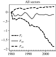
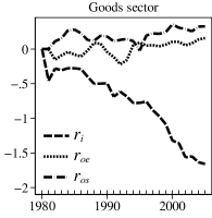
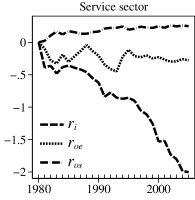
Figure A1: Rental prices of ICT equipment, non-ICT equipment, and non-ICT structures

Notes: The rental prices of ICT equipment, non-ICT equipment, and non-ICT structures are denoted by $r_{i}$, $r_{oe}$, and $r_{os}$, respectively. All the series are logarithmically transformed and normalized to zero in the year 1980. The 1980 values of $r_{i}$, $r_{oe}$, and $r_{os}$ are 0.97 (1.21), 0.20 (0.25), and 0.09 (0.06) in the goods (service) sector, respectively.

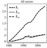
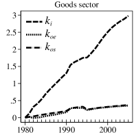
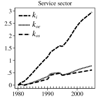
Figure A2: Quantities of ICT equipment, non-ICT equipment, and non-ICT structures

Notes: The quantities of ICT equipment, non-ICT equipment, and non-ICT structures are denoted by $k_{i}$, $k_{oe}$, and $k_{os}$, respectively. All the series are logarithmically transformed and normalized to zero in the year 1980. The 1980 values of $k_{i}$, $k_{oe}$, and $k_{os}$ are 4.95 (26.18), 266.83 (164.77), and 416.86 (1,709.65) billion U.S. dollars in the goods (service) sector, respectively.

A.3.3 Non-ICT equipment

The trends in the rental prices of capital differ significantly between ICT equipment and non-ICT structures but do not differ significantly between non-ICT equipment and non-ICT structures (Figure A1). The rental price of ICT equipment fell dramatically, but that of non-ICT equipment and structures remained almost unchanged in both the goods and services sectors. Meanwhile, the quantities of ICT equipment, non-ICT equipment, and non-ICT structures increased in both sectors. However, the rate of increase in ICT equipment is far greater than that in non-ICT equipment and structures for each sector (Figure A2). The rate of increase in non-ICT equipment is almost the same as that in non-ICT structures.

References

- (1)
- Acemoglu and Autor (2011) Acemoglu, Daron and David Autor (2011) “Skills, Tasks and Technologies: Implications for Employment and Earnings,” Handbook of Labor Economics, Vol. 4B, pp. 1043–1171.
- Acemoglu and Restrepo (2020) Acemoglu, Daron and Pascual Restrepo (2020) “Robots and Jobs: Evidence from US Labor Markets,” Journal of Political Economy, Vol. 128, No. 6, pp. 2188–2244.
- Acemoglu and Restrepo (2022) (2022) “Tasks, Automation, and the Rise in U.S. Wage Inequality,” Econometrica, Vol. 90, No. 5, pp. 1973–2016.
- Autor et al. (1998) Autor, David H., Lawrence F. Katz, and Alan B. Krueger (1998) “Computing Inequality: Have Computers Changed the Labor Market?” Quarterly Journal of Economics, Vol. 113, No. 4, pp. 1169–1213.
- Autor et al. (2003) Autor, David, Frank Levy, and Richard Murnane (2003) “The Skill Content of Recent Technological Change: An Empirical Exploration,” Quarterly Journal of Economics, Vol. 118, No. 4, pp. 1279–1333.
- Baqaee and Farhi (2019) Baqaee, David Rezza and Emmanuel Farhi (2019) “JEEA-FBBVA Lecture 2018: The Microeconomic Foundations of Aggregate Production Functions,” Journal of the European Economic Association, Vol. 17, No. 5, pp. 1337–1392.
- Barro and Lee (2013) Barro, Robert J. and Jong Wha Lee (2013) “A New Data Set of Educational Attainment in the World, 1950-2010,” Journal of Development Economics, Vol. 104, pp. 184–198.
- Beaudry and Lewis (2014) Beaudry, Paul and Ethan Lewis (2014) “Do Male–Female Wage Differentials Reflect Differences in the Return to Skill? Cross-city Evidence from 1980–2000,” American Economic Journal: Applied Economics, Vol. 6, No. 2, pp. 178–194.
- Black and Spitz-Oener (2010) Black, Sandra E. and Alexandra Spitz-Oener (2010) “Explaining Women’s Success: Technological Change and the Skill Content of Women’s Work,” Review of Economics and Statistics, Vol. 92, No. 1, pp. 187–194.
- Blackorby and Russell (1989) Blackorby, Charles and R. Robert Russell (1989) “Will the Real Elasticity of Substitution Please Stand Up? (A Comparison of the Allen/Uzawa and Morishima Elasticities),” American Economic Review, Vol. 79, No. 4, pp. 882–888.
- Blau and Kahn (2017) Blau, Francine D. and Lawrence M. Kahn (2017) “The Gender Wage Gap: Extent, Trends, and Explanations,” Journal of Economic Literature, Vol. 55, No. 3, pp. 789–865.
- Bound and Johnson (1992) Bound, John and George Johnson (1992) “Changes in the Structure of Wages in the 1980’s: An Evaluation of Alternative Explanations,” American Economic Review, Vol. 82, No. 3, pp. 371–392.
- Buera et al. (2022) Buera, Francisco J., Joseph P Kaboski, Richard Rogerson, and Juan I Vizcaino (2022) “Skill-Biased Structural Change,” Review of Economic Studies, Vol. 89, No. 2, pp. 592–625.
- Burstein et al. (2019) Burstein, Ariel, Eduardo Morales, and Jonathan Vogel (2019) “Changes in Between-group Inequality: Computers, Occupations, and International Trade,” American Economic Journal: Macroeconomics, Vol. 11, No. 2, pp. 348–400.
- Caunedo et al. (2023) Caunedo, Julieta, David Jaume, and Elisa Keller (2023) “Occupational Exposure to Capital-Embodied Technical Change,” American Economic Review, Vol. 113, No. 6, pp. 1642–1685.
- Chetty et al. (2011) Chetty, Raj, Adam Guren, Day Manoli, and Andrea Weber (2011) “Are Micro and Macro Labor Supply Elasticities Consistent? A Review of Evidence on the Intensive and Extensive Margins,” American Economic Review Papers and Proceedings, Vol. 101, No. 3, pp. 471–475.
- Comin et al. (2021) Comin, Diego, Danial Lashkari, and Martí Mestieri (2021) “Structural Change with Long-run Income and Price Effects,” Econometrica, Vol. 89, No. 1, pp. 311–374.
- Cummins and Violante (2002) Cummins, Jason G. and Giovanni L. Violante (2002) “Investment-specific Technical Change in the United States (1947–2000): Measurement and Macroeconomic Consequences,” Review of Economic Dynamics, Vol. 5, No. 2, pp. 243–284.
- Diamond et al. (1978) Diamond, Peter, Daniel McFadden, and Miguel Rodriguez (1978) “Measurement of the Elasticity of Factor Substitution and Bias of Technical Change,” Contributions to Economic Analysis, Vol. 2, pp. 125–147.
- Eden and Gaggl (2018) Eden, Maya and Paul Gaggl (2018) “On the Welfare Implications of Automation,” Review of Economic Dynamics, Vol. 29, pp. 15–43.
- Elsby et al. (2013) Elsby, Michael, Bart Hobijn, and Ayşegül Şahin (2013) “The Decline of the U.S. Labor Share,” Brookings Papers on Economic Activity, pp. 1–52.
- Fallon and Layard (1975) Fallon, P. R. and P. R. G. Layard (1975) “Capital–Skill Complementarity, Income Distribution, and Output Accounting,” Journal of Political Economy, Vol. 83, No. 2, pp. 279–302.
- Goldin and Katz (2010) Goldin, Claudia and Lawrence F. Katz (2010) The Race between Education and Technology: Harvard University Press.
- Greenwood et al. (1997) Greenwood, Jeremy, Zvi Hercowitz, and Per Krusell (1997) “Long-run Implications of Investment-specific Technological Change,” American Economic Review, Vol. 87, No. 3, pp. 342–362.
- Griliches (1969) Griliches, Zvi (1969) “Capital–Skill Complementarity,” Review of Economics and Statistics, Vol. 51, No. 4, pp. 465–468.
- Grossman and Oberfield (2022) Grossman, Gene M. and Ezra Oberfield (2022) “The Elusive Explanation for the Declining Labor Share,” Annual Review of Economics, Vol. 14, pp. 93–124.
- Hicks (1932) Hicks, John R. (1932) The Theory of Wages: Palgrave Macmillan London.
- Hornstein et al. (2005) Hornstein, Andreas, Per Krusell, and Giovanni L. Violante (2005) “The Effects of Technical Change on Labor Market Inequalities,” Handbook of Economic Growth, Vol. 1B, pp. 1275–1370.
- Johnson and Keane (2013) Johnson, Matthew and Michael P. Keane (2013) “A Dynamic Equilibrium Model of the US Wage Structure, 1968–1996,” Journal of Labor Economics, Vol. 31, No. 1, pp. 1–49.
- Jorgenson (1963) Jorgenson, Dale W. (1963) “Capital Theory and Investment Behavior,” American Economic Review Papers and Proceedings, Vol. 53, No. 2, pp. 247–259.
- Karabarbounis and Neiman (2014) Karabarbounis, Loukas and Brent Neiman (2014) “The Global Decline of the Labor Share,” Quarterly Journal of Economics, Vol. 129, No. 1, pp. 61–103.
- Katz and Murphy (1992) Katz, Lawrence and Kevin M. Murphy (1992) “Changes in Relative Wages, 1963–1987: Supply and Demand Factors,” Quarterly Journal of Economics, Vol. 107, No. 1, pp. 35–78.
- Keane and Rogerson (2012) Keane, Michael and Richard Rogerson (2012) “Micro and Macro Labor Supply Elasticities: A Reassessment of Conventional Wisdom,” Journal of Economic Literature, Vol. 50, No. 2, pp. 464–476.
- Krueger et al. (2010) Krueger, Dirk, Fabrizio Perri, Luigi Pistaferri, and Giovanni L. Violante (2010) “Cross-sectional Facts for Macroeconomists,” Review of Economic Dynamics, Vol. 13, No. 1, pp. 1–14.
- Krusell et al. (2000) Krusell, Per, Lee E. Ohanian, José-Víctor Rios-Rull, and Giovanni L. Violante (2000) “Capital–Skill Complementarity and Inequality: A Macroeconomic Analysis,” Econometrica, Vol. 68, No. 5, pp. 1029–1053.
- Lee and Wolpin (2006) Lee, Donghoon and Kenneth I. Wolpin (2006) “Intersectoral Labor Mobility and the Growth of the Service Sector,” Econometrica, Vol. 74, No. 1, pp. 1–46.
- McFadden (1963) McFadden, Daniel (1963) “Constant Elasticity of Substitution Production Functions,” Review of Economic Studies, Vol. 30, No. 2, pp. 73–83.
- Michaels et al. (2014) Michaels, Guy, Ashwini Natraj, and John Van Reenen (2014) “Has ICT Polarized Skill Demand? Evidence from Eleven Countries over Twenty-five Years,” Review of Economics and Statistics, Vol. 96, No. 1, pp. 60–77.
- Morishima (1967) Morishima, Michio (1967) “A Few Suggestions on the Theory of Elasticity,” Keizai Hyoron (Economic Review), Vol. 16, pp. 144–150.
- Niebel and Saam (2016) Niebel, Thomas and Marianne Saam (2016) “ICT and Growth: The Role of Rates of Return and Capital Prices,” Review of Income and Wealth, Vol. 62, No. 2, pp. 283–310.
- Oberfield and Raval (2021) Oberfield, Ezra and Devesh Raval (2021) “Micro Data and Macro Technology,” Econometrica, Vol. 89, No. 2, pp. 703–732.
- O’Mahony and Timmer (2009) O’Mahony, Mary and Marcel P. Timmer (2009) “Output, Input and Productivity Measures at the Industry Level: The EU KLEMS Database,” The Economic Journal, Vol. 119, No. 538, pp. F374–F403.
- Raveh (2015) Raveh, Ohad (2015) “Capital–Gender Complementarity,” Economics Bulletin, Vol. 35, No. 1, pp. 494–506.
- Sato (1975) Sato, Kazuo (1975) Production Functions and Aggregation: Elsevier.
- Taniguchi and Yamada (2022) Taniguchi, Hiroya and Ken Yamada (2022) “ICT Capital–Skill Complementarity and Wage Inequality: Evidence from OECD Countries,” Labour Economics, Vol. 76, 102151.
- Tinbergen (1974) Tinbergen, Jan (1974) “Substitution of Graduate by Other Labour,” Kyklos, Vol. 27, No. 2, pp. 217–226.
- Welch (2000) Welch, Finis (2000) “Growth in Women’s Relative Wages and in Inequality among Men: One Phenomenon or Two?” American Economic Review Papers and Proceedings, Vol. 90, No. 2, pp. 444–449.