Verification and Validation of Convex Optimization Algorithms for Model Predictive Control
Abstract
Advanced embedded algorithms are growing in complexity and they are an essential contributor to the growth of autonomy in many areas. However, the promise held by these algorithms cannot be kept without proper attention to the considerably stronger design constraints that arise when the applications of interest, such as aerospace systems, are safety-critical. Formal verification is the process of proving or disproving the "correctness" of an algorithm with respect to a certain mathematical description of it by means of a computer. This article discusses the formal verification of the Ellipsoid method, a convex optimization algorithm, and its code implementation as it applies to receding horizon control. Options for encoding code properties and their proofs are detailed. The applicability and limitations of those code properties and proofs are presented as well. Finally, floating-point errors are taken into account in a numerical analysis of the Ellipsoid algorithm. Modifications to the algorithm are presented which can be used to control its numerical stability.
Nomenclature
| = | The set of all real numbers. |
| = | Set of floating-point numbers. |
| = | The set of all positive real numbers. |
| = | The set of all strictly positive real numbers. |
| = | The set of real vectors of length . |
| = | The set of real matrices of size . |
| = | Frobenius norm of a matrix . |
| = | Two norm of a matrix . |
| = | Two norm of a vector . |
| = | n-dimensional unit Euclidean ball. . |
| = | Ball of radius centered on . . |
| = | Ellipsoid set defined by: . |
| = | Floating-point rounding of a given real number. |
| = | Model Predictive Control Horizon. |
| = | Condition number of a matrix . |
| = | Number of iterations. |
| = | Plant Input. |
| u = | Collection of input vectors to horizon: . |
| = | Volume of a given set. |
| = | Original Decision Vector for an Optimization problem. |
| = | Plant State Vector. |
| x = | Collection of state vectors to horizon: . |
| = | Feasible set of an optimization problem. |
| = | Epsilon optimal set of an optimization problem. |
| = | Projected Decision Vector for an Optimization problem. |
| = | Upper bound of Reduction Ratio. |
| = | Elevation Angle in Radians for the three degrees of freedom Helicopter. |
| = | Ellipsoids Widening Coefficient. |
| = | Largest singular value of a matrix . |
| = | Smallest singular value of a matrix . |
| = | Travel Angle in Radians for the three degrees of freedom Helicopter. |
| = | Pitch Angle in Radians for the three degrees of freedom Helicopter. |
1 Introduction
Formal verification of optimization algorithms used online within
control systems is the sole focus of this research. Recently, such algorithms have
been used online with great success for the guidance of safety-critical applications,
including, autonomous cars [1] and reusable
rockets [2].
The latter case has resulted in technology demonstrations such as the landings of SpaceX’s
Falcon 9 [3] and BlueOrigin’s New Shepard. Thus, algorithms solving optimization
problems are already used online, have been embedded on board, and yet
still lack the level of qualification required by civil aircraft or manned rocket flight.
Automatic code generation for solving convex optimization problems has already been done [4, 5],
but does not include the use of formal methods. Likewise, work within the field of model predictive
control already exists where numerical properties of algorithms are being evaluated
[6]. Nevertheless, this work is only valid for Quadratic Programming
(See Section 2) and using fixed-point arithmetic. As well, no formal verification is performed.
On the other hand, some contributions have been made concerning formal verification
of control systems [7, 8, 9, 10], but they
mainly focus on formal verification and code generation for linear control systems.
Research has also been made toward the verification
of numerical optimization algorithms [11, 12], yet it remains purely theoretical and
no proof was obtained using formal verification tools. Contributions on formal verification of optimization
algorithms have already been made [13], but this work focuses on a single optimization
problem, where closed-loop behaviors are not being addressed, which does not meet the level of guarantees
needed for receding horizon controllers.
As well, the formal proof was not complete and no numerical analysis was presented.
The need for enhanced safety and better performance is currently
pushing for the introduction of advanced numerical methods into the next generation of
cyber-physical systems. While most of the algorithms described in this article have been
established for a long time, their online use within embedded systems is relatively
new and introduces issues that have to be addressed. Among these methods, this study focuses
on numerical optimization algorithms.
The following scientific contributions are presented:
-
•
axiomatization of optimization problems and formalization of algorithm proof (Ellipsoid method) as code annotation
-
•
extraction of guarantees of convergence for sequential optimization problems, representing closed-loop management
-
•
modification of the original algorithm to account for floating-point errors
-
•
generation of C code implementations via credible autocoders of receding horizon controllers along with ANSI/ISO C Specification Language (ACSL) annotations
The choice of ellipsoid method here seems unconventional as current state of art solvers typically use some variant of the interior-point method. However it has been shown in [13] that guaranteeing the numerical accuracy of second-order methods are very challenging. This paper is a first attempt at providing methods and tools to formally verify convex optimization code for solving online receding-horizon control problems. The article is structured as follows: Section 2 presents backgrounds for convex optimization, model predictive control, and axiomatic semantics using Hoare triples. Section 3 focuses on the axiomatization of second-order cone programs and the formal verification of the Ellipsoid Method. Furthermore, the closed-loop management and the online aspect of the developed algorithm is discussed in Section 4. A modified version of the original Ellipsoid Method used to control floating-point errors, is presented in Section 5. A floating-point analysis of the ellipsoid method is presented in Section 6, while Section 7 presents how this framework can be automated and applied to a system, the three degrees of freedom (DOF) Helicopter. Finally, Section 8 concludes this article.
2 Preliminaries
2.1 Second-Order Cone Programming
Optimization algorithms solve a constrained optimization problem, defined by an objective function and a set of constraints to be satisfied:
| (1) |
This problem searches for , the optimization variable, minimizing , the objective function, while satisfying constraints , with associated bounds . An element of is feasible when it satisfies all the constraints . An optimal point is defined by the element having the smallest cost value among all feasible points. An optimization algorithm computes an exact or approximated estimate of the optimal cost value, together with one or more feasible points achieving this value. A subclass of these problems that can be efficiently solved are convex optimization problems. In these cases, the functions and are required to be convex [4], with one of the consequences being that a local minimizer is also a global minimizer. Furthermore, when the constraints are linear the problem is either called a Linear Program (LP) if the cost is also linear or called a Quadratic Program (QP) if the cost is quadratic. Optimization problems where both the cost and the constraints are quadratic are called Quadratically Constrained Quadratic Program (QCQP). Semi-Definite Programs (SDP) represent problems that have constraints which can be formulated as a Linear Matrix Inequality (LMI). Here, only a specific subset of convex optimization problems are presented in details: Second-Order Cone Programs (SOCPs). For , a SOCP in standard form can be written as:
| (2) |
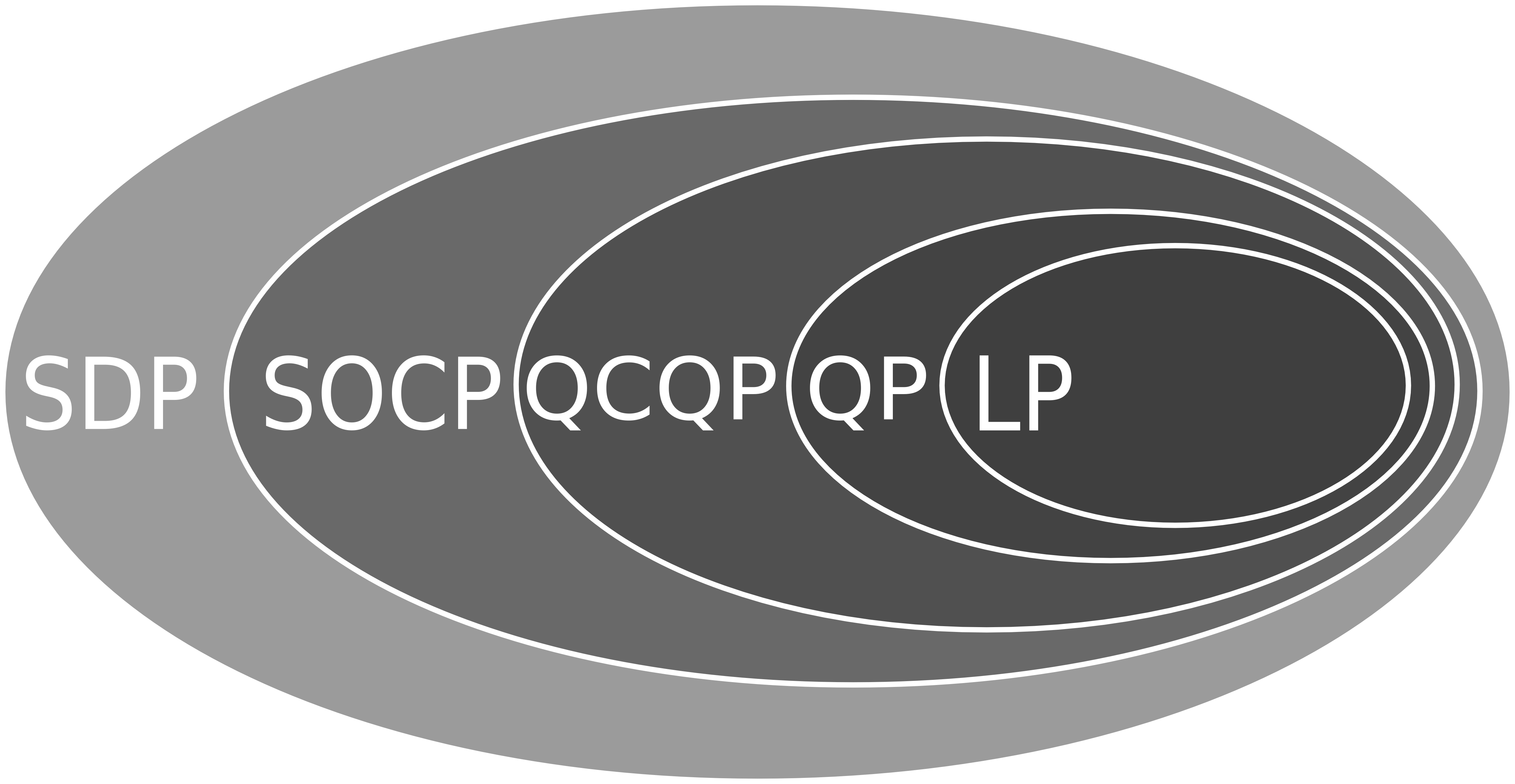
A classification of the most common convex optimization problems is presented in Fig. 1. Frequently, optimization problems that are used online for control systems can be formulated as a SOCP. Furthermore, extensions to SDPs are possible with little additional work. The algorithm used and the proof are still valid for any convex problem.
2.2 Model Predictive Control (MPC)
Model predictive control (also known as receding horizon control) is an optimal control strategy based on numerical optimization. In this technique, a discrete-time dynamical model of the system is being used to predict potential future trajectories. As well, a cost function, that depends on the future control inputs and states, is being considered over the receding prediction horizon , with the objective being to minimize this cost. At each time , a convex optimization problem is being solved and the corresponding input is sent to the system. A time step later, the exact same process occurs and is repeated until a final time. We refer the reader to [14, 15] for more details on MPC.
2.3 Axiomatic Semantics and Hoare Logic
Semantics of programs express their behavior. Using axiomatic semantics, the program’s semantics can be defined in an incomplete way, as a set of projective statements, i.e., observations. This idea was formalized by [16] and then [17] as a way to specify the expected behavior of a program through pre- and post-conditions.
Hoare Logic.
A piece of code is axiomatically described by a pair of formulas such
that when holds before executing , then should be valid after its
execution. This pair acts as a contract for the function and is called
a Hoare triple. In most uses, and are expressed in first order formulas
over the variables of the program. Depending on the level of precision of these
annotations, the behavior can be fully or partially specified. In our case we
are interested in specifying, at code level, algorithm specific properties such
as the algorithm convergence or preservation of feasibility for
intermediate iterates.
Software analyzers, such as the Frama-C platform [18],
provide means to annotate source code with these contracts, and tools to
reason about these formal specifications.
For the C language, ACSL [19]
(ANSI C Specification Language) can be used to write source comments.
Figure 2 shows an example of a function contract expressed in ACSL. The \sayensures keyword expresses all the properties that will be true after the execution of the function, assuming that all the properties listed within the \sayrequires keywords were true before the execution (similar to a Hoare triple). As well, it is possible to annotate and check the part of the memory assigned by a function using the keyword \sayassigns. In the case shown in Fig. 2, the function is not assigning anything during its execution, and therefore no global variable were changed. Throughout this article, the verification is performed using the software analyzer Frama-C and the SMT solver (Satisfiability Modulo Theories) Alt-Ergo [20], via the Weakest Precondition (WP) plug-in. The role of the WP plug-in is to implement a weakest precondition calculus for ACSL annotations present at code level. For each annotation, the WP plug-in generates proof obligations (mathematical first-order logic formulas) that are then submitted to Alt-Ergo. Further information about the WP plug-in can be found in [21].
3 Formal Verification of an Ellipsoid Method C code Implementation
Our goal is to build a framework that is capable of compiling the
high-level requirements of online MPC solvers into ACSL augmented C code
which can then be automatically verified using existing formal methods
tools for C programs such as Frama-C and Alt-ergo.
The MPC solver shall take a parameterized SOCP problem as inputs and
always outputs a solution that is both feasible and epsilon-optimal
within a predefined number of iterations.
This kind of requirement has never been formalized before.
Hence it also has never been verified by the state of art automatic
formal methods techniques and it is not really possible to do so
without going into some manual proofs. To formalize these high-level
requirements, one has to:
-
•
formalize in ACSL the low-level types, such as vectors and matrices
-
•
formalize in ACSL second-order cone problems
-
•
formalize the solver (from algorithm and input problem to the generated C code)
-
•
formalize the properties of the ellipsoid method in a way such that they can be expressed as axiomatic semantic of the C program (ACSL types, axioms, functions to express feasability and optimality).
For example, mathematical types from linear algebra can be defined axiomatically. The input problem and solver choice is automatically transformed into a C program. The high-level properties (feasability and optimality) of the chosen solver together with the input problem are compiled into an ACSL form (expressing the axiomatics semantics of the generated C program), and then inserted into the C program as comments. The various artifacts (ACSL types, functions, predicates, axioms, lemmas, theorems), that were manually written to support the compilation of the high-level requirements (HLR) into C+ACSL and its automatic verification, are packaged into libraries. Examples of these artifacts include types like matrix, vector, optim, predicates like \sayisFeasible and functions such as \saytwoNorm, etc.
3.1 Semantics of an Optimization Problem
The first work to be done is the formal definition of an optimization problem.
In order to do so, new mathematical types, objects, axioms and theorems are created.
Our goal is to axiomatize optimization problems with enough properties allowing
us to state all the needed optimization-level properties at code level.
Let us consider the second-order cone program, described in Eq. (2).
Encoding an SOCP. In order to fully describe an SOCP, we use the variables:
The vector is used to collect the sizes of the vectors . Furthermore, if , then the SOCP (2) is an LP. Using ACSL, a new type and a high level function are defined, providing the possibility to create objects of the type \say. Figure 3 represents an extract of the ACSL optimization theory. First, a new ACSL theory is created using the keyword \sayaxiomatic. The keyword \saylogic is used to define a new function and its signature. Information about the part of memory used by a function is provided using the keyword \sayreads. Figure 3 presents the definition of 2 functions. The function is used to instantiate objects representing an optimization problem of appropriate sizes.
The function returns a vector collecting the values of all the constraint functions for a given problem and point. When applying a method to solve an actual optimization problem, many concepts are crucial. The work here is to highlight the parts of the HLR that need to be formalized (via axiomatization) and packaged into a library to support the automatic compilation of the HLR into ACSL augmented C code. The concepts of feasibility and optimality are being axiomatized. For this, given a second-order cone program, an axiomatic definition is given for the vector constraint, the gradient of a constraint, the cost, optimal point (making the assumption that it exists and is unique), etc. For instance, Fig. 4 illustrates the axiomatization of a constraint calculation and the feasibility predicate definition. For the constraint calculation, two axioms are defined representing two different cases: The case where the constraint is linear and the case where it is not. The predicate shown in Fig. 4 defines that a point is feasible if all the components of its constraint vector are negative.
When instantiating an object of type vector or matrix, the size of the considered object needs to be known since it is hard-coded in the ACSL axiomatization. This is not an issue since at this time (post parsing), all the sizes of the variables used are already defined. The objects sizes only depend on the plant’s order and the horizon. Thus, as long as the order of the plant and the horizon do not change dynamically, the variables sizes can be predicted. Also, working with predefined and hard-coded size objects will help the analyzers proving the goals.
3.2 The Ellipsoid Method
Despite its modest efficiency with respect to interior point methods, the Ellipsoid Method [22, 23, 24] benefits from concrete proof elements and could be considered a viable option for critical embedded systems where safety is more important than performance. This section presents a way to annotate a C code implementation of the Ellipsoid Method. Before recalling the main steps of the algorithm, some mathematical preliminaries are presented.
Ellipsoids in .
An ellipsoid can be characterized as an affine transformation of an Euclidean Ball. Before defining an Ellipsoid set, the definition of an Euclidean ball is first recalled.
Definition 1 (Euclidean ball)
Let , denotes the unit Euclidean ball in . represents its volume. As well, is defined as the ball of radius centered on ( i.e ).
Definition 2 (Ellipsoid Sets)
Let and , be a non-singular matrix (). The Ellipsoid is the set :
| (3) |
Definition 3 (Volume of Ellipsoids)
Let be an ellipsoid set in . denotes its volume and is defined as :
| (4) |
Algorithm.
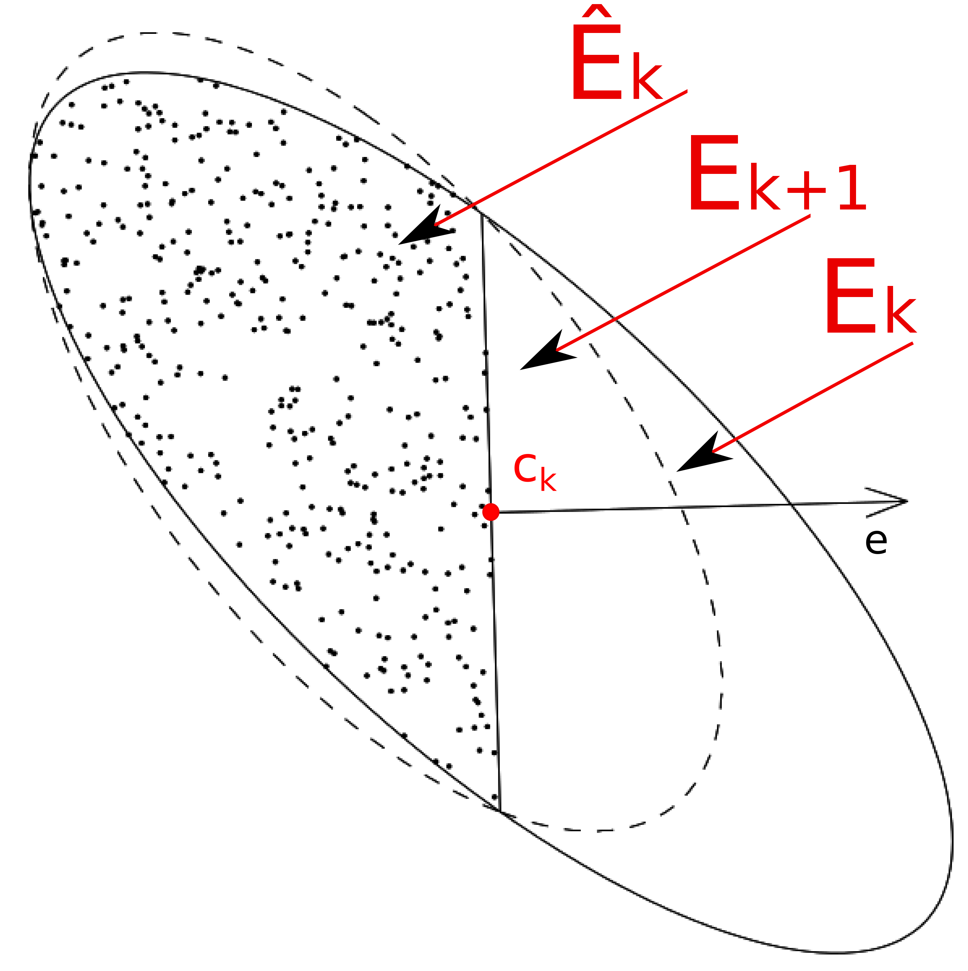
Ellipsoid cut.
The algorithm starts with an ellipsoid containing the feasible set , and therefore the optimal point . An iteration consists of transforming the current ellipsoid into a smaller volume ellipsoid that also contains . Given an ellipsoid of center , the objective is to find a hyperplane containing that cuts in half, such that one half is known not to contain . Finding such a hyperplane is called the oracle separation step, cf. [24]. Within the SOCP setting, this cutting hyperplane is obtained by taking the gradient of either a violated constraint or the cost function. Then, the ellipsoid is defined by the minimal volume ellipsoid containing the half ellipsoid that is known to contain . The Fig. 5(a) and 5(b) illustrate such ellipsoids cuts.
Ellipsoid transformation.
From the oracle separation step, a separating hyperplane, , that cuts in half with the guarantee that is localized in has been computed. The following step is the Ellipsoid transformation. Using this hyperplane , one can update the ellipsoid to its next iterate according to Eqs. (5),(6) and (7). In addition to that, an upper bound, , of the ratio of to is known.
| (5) |
| (6) |
with:
| (7) |
Termination.
The search points are the successive centers of the ellipsoids. Throughout the execution of the algorithm, the best point so far, is being stored in memory. A point is better than a point if it is feasible and has a smaller cost. When the program reaches the number of iteration needed, the best point so far, , which is known to be feasible and -optimal, is returned by the algorithm. A volume related property is now stated, at the origin of the algorithm convergence, followed by the main theorem of the method. Both properties can be found in [24, 26].
Property 1
[Reduction ratio.] Let , by construction:
| (8) |
Please find below the the proof of this property.
Proof 1
Necessary Geometric Characteristics.
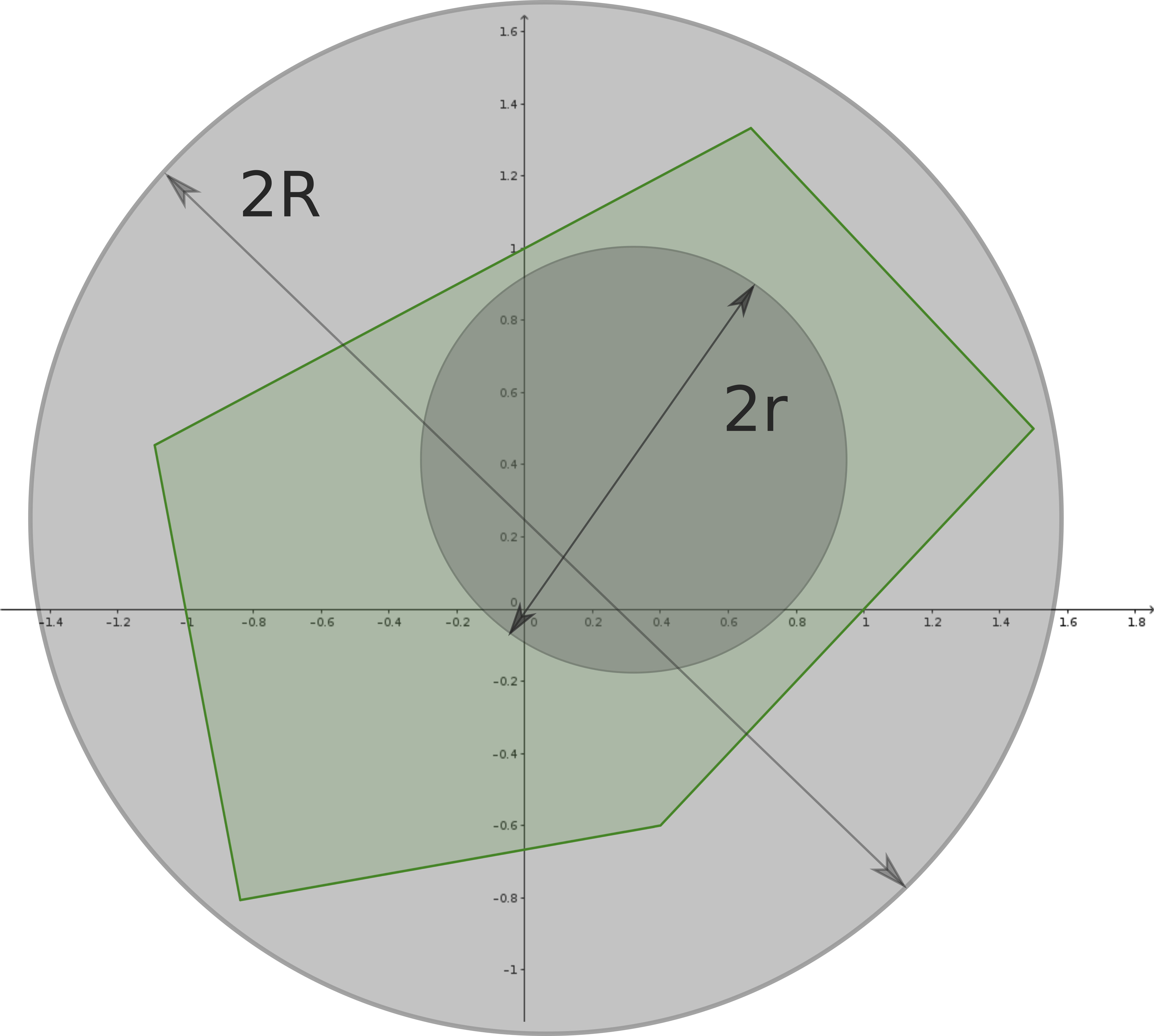
In order to know the number of steps required for the algorithm to return an -optimal solution, three scalars and a point are needed:
-
•
a radius such that
(9) -
•
a scalar such that there exists a point such that
(10) -
•
and another scalar such that
(11)
Figure 6 illustrates the scalars and . The
Feasible set (assumed to be bounded) is shown in green.
The main result can be stated as:
Theorem 1
This result, when applied to LP, is the first proof of the polynomial solvability of
linear programs. This proof can be found
in [24, 26].
3.3 ACSL Theory
This section would be to describe all the manually written ACSL artifacts to support the automatic formalization and then verification of the HLR. Indeed, the software analyzer takes as an input the annotated C code plus ACSL theories that define new abstract types, functions, as well as axioms, lemmas and theorems. The lemmas and theorems need to be proven but the axioms are taken to be true. For the SMT solver, properties within C code as annotations are usually harder to prove than lemmas within an ACSL theory. On top on checking the mathematical correctness of an ACSL annotation, the SMT solver needs to check the soundness of the code itself (e.g., memory allocation, function calls, ACSL contracts on the function called, etc). Thus, the approach chosen here is to develop as much as possible the ACSL theories to express and prove the main results used by the algorithm. That way, the Hoare triples at code level are only an instantiation of those lemmas and are relatively simple to prove.
Linear Algebra Based ACSL Theory.
In this ACSL theory, new abstract
types for vectors and matrices are defined. Functions allowing the instantiation
of those types of objects are also defined. As well, all of the well-known
operations have also been axiomatized, such as vector-scalar multiplication, scalar product, norm etc.
This ACSL theory is automatically generated during the autocoding
process of the project and all the sizes of the vectors and matrices are known.
Thus, within this theory, only functions that will create
objects, from a C code pointer, of appropriate sizes (as illustrated in
Fig. 7) are being defined. ACSL code is printed in green and its keywords
in red. The C code keywords are printed in blue and the actual C code is
printed in black. Using the keyword \saytype, two new abstract types, matrix and vector
are being defined. Furthermore, the ACSL constructors for those
types and the axiomatization of vector addition is shown in Fig. 7.
The first axiom states that the length of the addition of two vectors, of same length is
equal to this same length. The second axiom states that the elements of the
addition of two vectors is the addition of the elements of the two separate vectors.
Figure 7 shows a partial sample of the autocoded ACSL linear
algebra theory.
Optimization and Ellipsoid Method Based ACSL Theory.
The axiomatization of optimization problems has already been briefly discussed in Section 3.1. Additionally, work has been dedicated to axiomatize the calculation of the vector constraint, feasibility, epsilon-optimality, etc. As well,
Ellipsoids and related properties are formally defined, such as those presented in Fig. 8. Figure 8 presents the definition of another theory called \sayEllipsoid and within it, it shows the creation of a new abstract type \sayellipsoid and the definition of the functions \sayEll and \sayinEllipsoid. The function \sayEll returns the Ellipsoid formed by the matrix and vector as defined in Eq. (3). The function \sayinEllipsoid returns true if the vector is in the Ellipsoid and returns false otherwise. As it was explained earlier, Theorem 1 was translated to ACSL and auto generated as ACSL lemmas. All the autocoded lemmas are proven using the software analyzer Frama-C and the SMT solver Alt-Ergo. One of the autocoded lemmas can be found in Fig. 9 and can be expressed using common mathematical notations as:
A formal definition is also given for a point being better than another point . The set represents the set obtained by shrinking the feasible set by a factor centered on the optimal point . Further details about this set can be found in [24].
3.4 Annotating C Code
Details are now given about how the C code is annotated and the type of Hoare triples used. For this, a specific technique was adopted. Every C code function is implemented in a separated file. That way, for every function, a corresponding C code body (.c) file and header file (.h) are automatically generated. The body file contains the implementation of the
function along with annotations and loop invariants. The header file contains the declaration of the function with its ACSL contract. The first kind of Hoare triples and function contracts added to the code were to check basic mathematical operations. Figure 11 shows an ACSL contract relative to the C code function computing the 2-norm of a vector of a size two. The ACSL contract specifies that the variable returned is positive and equal to the 2-norm of the vector of size two described by the input pointer. Using the keywords \saybehavior, \saydisjoint and \saycomplete one can specify the different scenarios possible and treat them separately. Furthermore, it is proved that the result is always positive or null, and assuming the corresponding input vector not equal to zero, the output is strictly greater than zero. This last property becomes important when one must prove there are no divisions by zero (normalizing vectors). The implementation of the function is presented in Fig. 11. Once all the C functions implementing elementary mathematical operations have been annotated and proven, the next step consists of annotating the higher level C functions such as constraint and gradient calculations, matrix and vector updates, etc. Please find in Fig. 12 as an example, the annotated C function for the function \saygetp that computes the vector as described in Eq. (7), needed to perform the ellipsoid update.
In Fig. 12 one can note the presence of several function calls followed by ACSL annotations, encoding the corresponding specifications. The first function call refers to the function \saygetTranspose which computes the transpose of the matrix \sayP_minus and stores it into the variable \saytemp_matrix. The function \saychangeAxis multiplies the matrix \saytemp_matrix by the vector \saygrad and stores the result into the vector \saytemp2. The current state of the memory is specified at each line of code using ACSL annotations. Then, after computing the norm and scaling the vector \saytemp2, the annotations specify that the resulting vector stored in the variable has indeed been calculated as stated in Eq. (7).
4 Sequential Optimization Problems
In this section, convergence guarantees are provided
for a class of optimization problems used online.
For this, an optimization problem with parameterized constraints
and cost will be considered.
This section concerns the study of how this
parameter affects the optimization problem at each iteration and
how to find the condition that the parameter needs to satisfy in order to prove
convergence for every point along the trajectory.
First, the study focuses on the special case of linear constraints. Following this,
another section will be dedicated to SOCP constraints.
4.1 Parameterized Linear Constraints
The objective is to solve in real-time the optimization problem described in Eq. (12). The vector denotes the decision vector.
| (12) | ||||||
| subject to |
The initialization of this optimization problem is done using Eq. (13), where is a full rank matrix. Usually, represents a selector matrix and is of the form: . A selector matrix is a matrix that selects one or more component from . If is a selector matrix then returns certain components of . In that case it is obviously full rank. denotes the input of the controller and it is written to account for the fact that changes from one optimization problem to another.
| (13) |
One can decompose and separate the equality and inequality constraints hidden behind the matrix and vector . That way, Eq. (12) can be written as:
| (14) | ||||||
| subject to | ||||||
The idea here is to project all the equality constraints in order to eliminate them while keeping track of the variable parameter, . There exist matrices , and such that for all vectors satisfying the equality constraints of the problem defined by Eq. (14), there exists a vector such that:
| (15) |
Equation (15) is a direct implication that the set of solutions of a linear system is an affine set. In this same equation, is a matrix formed by an orthonormal basis of the null space of the matrix and denotes the total number of equality constraints (number of rows of + number of rows of ). The vector then belongs to with . Thus, the original optimization problem described by Eq. (12) is equivalent to the projected problem:
| (16) | ||||||
| subject to |
With:
| (17) |
More details and references about equality constraints elimination can be found
in [4]. Using the Ellipsoid Method online to solve this optimization problem
requires the computation of geometric characteristics on the feasible set of this parametric
optimization problem for every possible . For that reason, for now, let us assume:
.
The parameterized polyhedral set below is defined as:
| (18) |
Having this collection of polyhedral sets, the goal is to compute ball radii that will tell us about the volume of the feasible set that would be true for every . The operator returns for a matrix the vector whose coordinates are the 2-norm of the rows of . Thus, a way of computing those geometric characteristics is to consider the two extreme polyhedral sets below:
| (19) |
| (20) |
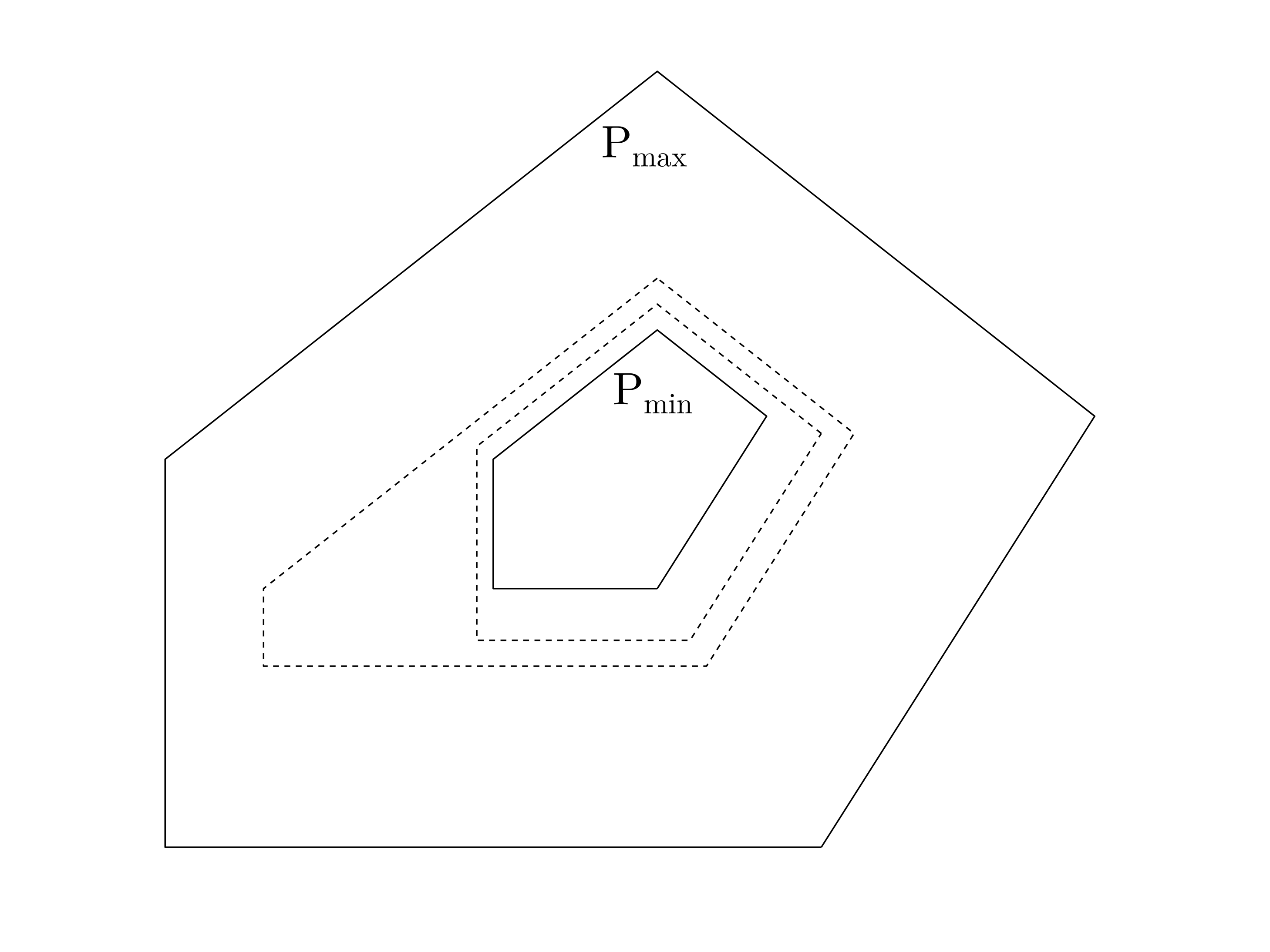
In order to give an example of this concept, please find in Fig. 13
an illustration of such polyhedral sets (the illustrated sets have no
physical meaning and do not represent any MPC problem).
The two extreme polyhedral sets are drawn with solid lines and
the actual feasible polyhedral sets are drawn using dotted lines.
The values used are:
Fact 1
[Extreme Polyhedral Sets]
Proof 2
Take such that .
First, using the Cauchy-Schwarz inequality, one can write:
| (21) |
Then, if , one can conclude that . Using the inequality above, it is clear that it implies . Similarly, assuming that and using the inequality below, it is clear that .
Next, one needs to find three scalars and such that:
| (22) |
| (23) |
| (24) |
For the first scalar, , one can compute a numerical value by running an
off-line optimization problem finding the largest ball inside . If no solution
can be found, the value of needs to be decreased, and the process is repeated until
acceptable values for and are found. Further information
about finding the largest ball in a polytope can be found in [4].
As a consequence of equality constraint elimination, and seen in Eq. (15),
the relation between the original decision vector and the
projected vector can be written as:
| (25) |
The decision vector can now be decomposed into two parts, x and u. The part u is bounded due to constraints in the original optimization problem (described by Eq. (12)). If no constraints on u were originally present, one can construct bounds on the projected vector to make the problem bounded and simpler to analyze. The point here being that from bounded variables within the vector , one can infer bounds on the projected vector . There is no need to have original bounds specifically on the collection of future inputs. Rewriting Eq. (25) yields:
| (26) |
Following this, one can conclude:
| (27) |
Therefore assuming again that , one can compute a value of such that:
| (28) |
On the other hand, from the physical meaning of the variables and the constraints of the
optimization problem, one can construct bounds in which the variables should live, and
therefore find a lower bound for .
With the values and , one can now guarantee the convergence of a family of optimization problems parameterized by .
Theorem 2
[MPC Ellipsoid Method Convergence]
The problem given by Eq. (14) is run in an online
fashion in order to implement receding horizon control.
Using the Ellipsoid Method and initializing the first Ellipsoid by ,
the method will find an -solution using iterations for all such that
, with:
with the variables , , and satisfying the Eqs. (22), (23) and (24). The variable denotes the dimension of the parameterized optimization problem.
Proof 3
. Let us assume, the problem given by Eq. (14) is run online. For each iteration, the input parameter is assumed to satisfy . denotes the feasible set of the current optimization problem to solve. That way, Eq. (22) is satisfied. Thus, by definition of , we know that:
Similarly, because it is assumed that satisfies Eq. (23), the following property holds:
As well, the scalar satisfies Eq. (11). Finally, One can conclude that the returned point will indeed be -optimal using iterations thanks to Theorem 1.
Linear Programs: In the case of Linear Programs, the method developed is identical and having a linear cost, the scalar is easily found by running the two optimization problems below.
4.2 Second-Order Conic Constraints
In the last section, the fact that only linear constraints was present was used to find the radius . Therefore, in this section we aim to give ways of computing these constants for second-order constraints. Consider that one wants to solve a model predictive control optimization problem given by Eq. (29).
| (29) | ||||||
We assume that no equality constraints are hidden in the second-order constraints (if not, a very simple analysis will confirm this and one can extract those equality constraints and put it into the couple from equation (29)). Performing again an equality constraint elimination, we end up with an equivalent optimization problem, of smaller dimension, that contains no equality constraint. We want to find the radius of the biggest ball inside the feasible set of this latter problem. Unfortunately, second-order constraints are still present and finding the largest balls inside second-order cones is not an easy task. For this, we use the equivalence of norms in finite dimensions, noting that and are linear, to perform a linear relaxation on the second-order constraints and end up with a polyhedral set as the feasible set. For instance, the problem described by Eq. (30) represents a linear relaxation of the original problem stated in Eq. (29) after having eliminated the equality constraints.
| (30) | ||||||
Thus, by finding the largest ball inside the resulting feasible set (which is a polyhedral set), a ball is finally found inside the original second-order cone.
5 Bounding the Condition Number
The use of the Ellipsoid Method was justified by arguing that it represents a trade off between performance and safety. As well, it also attracted our attention for its numerical properties. Although at first, the Ellipsoid Method appears to be numerically stable, finding a priori bounds on the program’s variables is challenging. The worst case occurred when the separating hyperplane has the same direction at each iteration. In this case, the condition number of the successive ellipsoids increases exponentially, and so do the program’s variables. This worst case is very unlikely to happen in practice. Nevertheless, a mathematical way to get around this case is needed, along with a way to compute a priori bounds on the variables before the execution of the program. In this section, a method for controlling the condition number of the successive ellipsoids and a way to compute those bounds by adding a correcting step in the original algorithm is presented. This section also includes how the formal proof of the corresponding software is modified to support the correctness of the resulting modified ellipsoid algorithm.
5.1 Bounding the Singular Values of the Successive Ellipsoids
When updating by the usual formulas of the ellipsoid
algorithm (Eq. (6)), evolves according to
, where has singular values equal
to , and has
one singular value equal to .
It follows that at a single step the largest and the smallest
singular values of can change by a factor from
.
The objective is to prove that one can modify the algorithm to
bound the singular values of the matrix
throughout the execution of the program.
Minimum Half Axis: First, we claim that if is
less than than then the algorithm has already found an
-solution. Note that the scalar is the desired precision and the scalars and
are defined in Section 3. Please find below a proof of this
statement.
Proof 4
Let us assume . In this case, is contained in the strip between two parallel hyperplanes, the width of the strip being less than and consequently does not contain , where is the minimizer of and (because contains a ball of radius ). Consequently, there exists such that but , implying by the standard argument (developed in [24]) that the best value of processed so far for feasible solutions satisfies which implies that . We can thus stop the algorithm and return the current best point found (feasible and smallest cost).
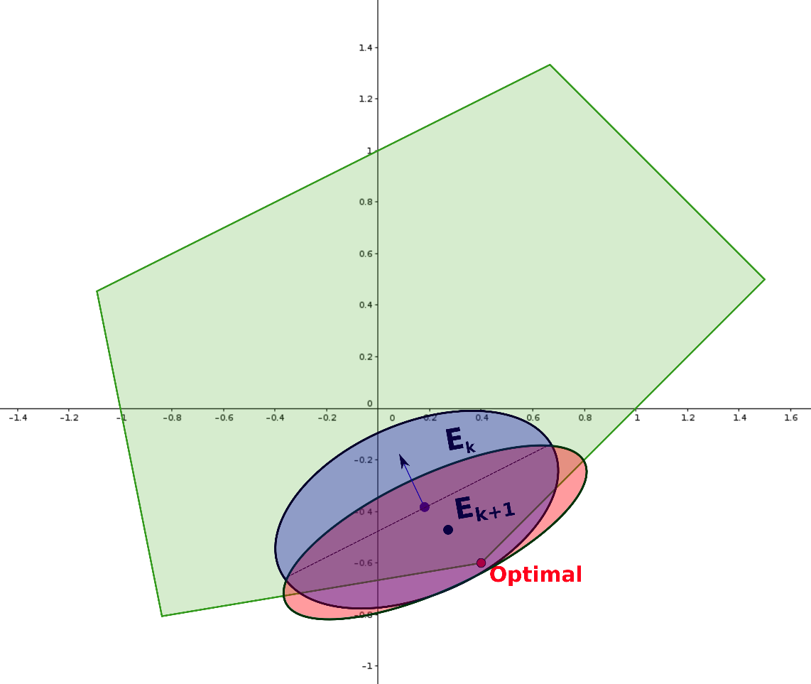
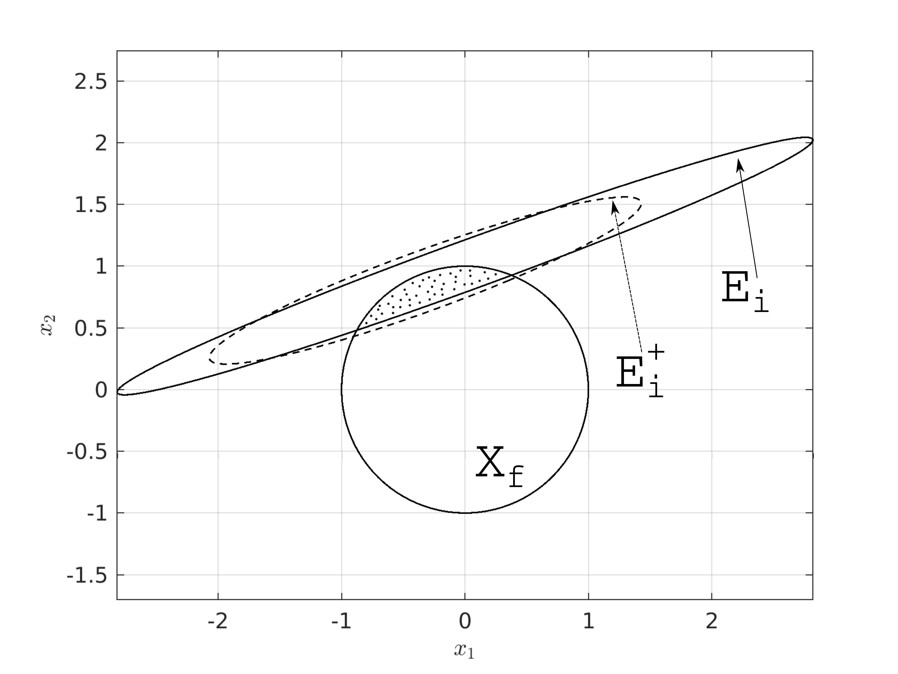
Maximum Half Axis: We argue now that one can modify the original ellipsoid algorithm in order to bound the value of the maximum singular value of . When the largest singular value of is less than , we carry out a step as in the basic ellipsoid method. When this singular value is greater than , a corrective step is applied to , which transforms into . Under this corrective step, is a localizer along with , specifically , and additionally:
-
(a) The volume of is at most (upper bound of reduction ratio from Eq. (8)) times the volume of ;
-
(b) The largest singular value of is at most .
The corrective step is described as follows. First, define and let be a unit vector corresponding to the singular direction. We then consider:
This case is concluded by performing the update:
| (31) |
Please find in Fig. 14 an illustration of this corrective step. The ellipsoid shown in Fig. 14 appears to have a condition number too high due to its large semi-major axis. The correction step as detailed previously has been performed and the corrected ellipsoid is shown with dotted line. As one can see, the volume as been decreased and the area of interest (dotted area) still lies within the ellipsoid . Hence, one can conclude that throughout the execution of the code:
5.2 Corresponding Condition Number
From the definition of the condition number, one can write:
Thus, by bounding the singular values of , a bound on its condition number can be constructed. The factors and that could affect the singular values of at each iteration are also taken into account to get:
and
5.3 Corresponding norm on
At each iteration it is known that the optimal point belongs to the current ellipsoid. Thus:
Finally,
5.4 Consequences on the Code
In this section, we explain how to implement this correcting step and give the tools to verify it. In order to detect an ellipsoid with large semi-major axis, the largest singular value of the current matrix needs to be computed. However, performing a singular value decomposition would be far too expensive and slow (this decomposition being performed at each iteration). The Frobenius norm, defined in Def. 4, which is a well-known upper bound on the maximum singular value, is computed instead.
Definition 4
The Frobenius norm of a matrix is:
The Frobenius norm of a vector has been axiomatized by setting it equal to the vector 2-norm of the \sayvectorized matrix. A matrix is \sayvectorized by concatenating all its rows in a single vector. In the case of an overly large semi-major axis, the direction in which this axis lies is needed as well. Therefore, the power iteration algorithm is performed in order to compute this information.
6 Floating-Point Considerations
Standard notation is used for rounding error
analysis [27, 28, 29], being the result
of the expression within the parenthesis rounded to the nearest floating-point number.
The relative rounding error unit is written u and eta denotes
the underflow unit. For IEEE 754 double precision (binary64) we have u
and eta.
This section presents an analysis targeting the numerical properties
of the ellipsoid algorithm. Contributions already have been made concerning
finite-precision calculations within the ellipsoid method [26].
However, this work only shows that it is possible to compute approximate solutions without
giving exact bounds, and is only for Linear Programming (LP).
Also, the analysis performed considers abstract
finite-precision numbers and the actual machine floating-point types are not mentioned. Thanks to the
analysis performed in this section, using the IEEE standard for floating-point
arithmetic and knowing exactly how the errors are being propagated, it is possible to check
a posteriori the correctness of the analysis using static
analyzers [30, 31].
6.1 Preliminaries
Within this algorithm, we focus our attention on the update formulas (5), (6) and (7), allowing us to update the current ellipsoid into the next one. In order to propagate the errors due to rounding through the code, we state now a useful theorem dealing with matrix perturbations and inverses.
Theorem 3
[32][Matrix perturbations and Inverse] Let be a non-singular matrix of and a small perturbation of . Then,
| (32) |
6.2 Norms and Bounds
To successfully perform the algorithm’s numerical stability analysis, we need to know how \saybig the variables can grow within the execution of the algorithm. Indeed, for a given computer instruction, the errors due to floating-point arithmetic are usually proportional to the variables values. As it was explained in Section 5, we slightly modified the ellipsoid algorithm to keep the condition numbers of the ellipsoid iterates under control. Therefore, implementing this corrected algorithm, we can use the following results:
| (33) |
| (34) |
| (35) |
| (36) |
where and are the variables described in Section 3.
6.3 Problem Formulation and Results
In order to take into account the uncertainties on the variables due to floating-point rounding, the algorithm is modified to make it more robust. Those uncertainties are first evaluated and a coefficient is then computed. This coefficient represents how much the ellipsoid is being widened at each iteration (see Fig. 15). Let us assume we have , , . We want to find such that:
| (37) |

Before evaluating any of those rounding errors, Lemma 1 is stated, which gives a sufficient condition for the coefficient to have covering . If the calculations of and were perfect, using Lemma 1, would be a solution; no correction is indeed necessary.
Lemma 1
[Widening - Sufficient Condition]
Proof 5
The starting hypothesis is: . Using the fact that the two norm is a consistent norm, we have:
Therefore using these properties and the assumed starting property, we have:
Then, using the triangle Inequality (), we finally have:
Reformulating the second part of the above statement (we are assuming that ):
Using the definition of Ellipsoids described in Eq. (3), one can write the equivalent statement:
Rearranging the equation implies:
Again, this is equivalent to:
which is the desired property:
The floating-point errors , and are defined as:
| (38) |
For now, it is assumed that after performing the floating-point analysis, and have been found such that:
From Lemma 1, one can see that the
calculation of a widening coefficient highly depends on the accuracy
of the matrix . Therefore,
is also needed such that: .
The quantity is not used explicitly in the
algorithm and its floating-point error could not be evaluated
by numerically analyzing the method.
Instead, perturbation matrix theory [32]
and Theorem 32 will be used, which gives a lower bound
on given , the norm of
and its condition number. The result is stated as follows.
Lemma 2
[Widening - Analytical Sufficient Condition]
Proof 6
Thus, due to Lemma 2, following the floating-point analysis of the algorithm, a coefficient such that Eq. (37) is valid can now be computed. After finding such a , using over-approximation schemes, we consider how the algorithm’s convergence changes. Because the method’s proof lies with the fact that the final ellipsoid has a small enough volume, this correction has an impact on the guaranteed number of iterations. Lemma 40 addresses those issues.
Lemma 3
[Convergent Widening Coefficient]
Let .
The algorithm implementing the widened ellipsoids, with coefficient converges if:
| (39) |
In that case, if denotes the original number of iteration needed, the algorithm implementing the widened ellipsoids will require:
| (40) |
Proof 7
We recall that the Ellipsoid algorithm implementing the widened ellipsoids, with coefficient converges if:
When using the Ellipsoid algorithm update process (with or without condition number correction), we have:
With , and Eq. (4), we know that:
Therefore, the algorithm implementing the widened ellipsoids, with widening coefficient will converge if:
Proof 8
The second statement of Lemma 40 is now proved, which shows how to compute the updated number of iterations for the algorithm implementing widened ellipsoids. We introduce . Therefore using Eq. (4), and , we get:
To end up at the final step with an ellipsoid of the same volume, we need: . Which implies
Replacing by its value, using property 8 from Section 3.2:
And thus, we arrive at the formula:
6.4 Computing and
This section introduces the evaluation of the floating-point errors taking place
when performing the update formulas (5) and (6)
(represented by and ).
For this, numerical properties for basic operations appearing in the algorithm
are first presented.
Rounding of a Real. Let ,
Product and Addition of Floating-Points. Let .
Reals-Floats Product. Let and ,
Scalar Product. Let . We define, and . We have then:
Rounding Error on .
Knowing how the errors are being propagated through elementary transformations, the goal is to compute the error for a transformation similar to the vector ’s update. For each component of , we have:
Therefore, the operation performed, in floating-point arithmetic is:
| (41) |
Using this and neglecting all terms in eta and powers of u greater than two, we get:
| (42) |
Error on .
Similarly, for each component of , the operation below is performed:
In floating-point arithmetic, this last equation can be put into form:
Similarly, propagating the errors using elementary transformations implies that:
| (43) |
7 Automatic Code Generation and Examples
7.1 Credible Autocoding
Credible autocoding, is a process by which an implementation of a certain input model in a given programming language is being generated along with formally verifiable evidence that the output source code correctly implements the input model. The goal of the work presented in this article is to automatically generate, formally verifiable C code implementations of a given receding horizon controller. Thus, an autocoder that we call a \sayCredible Autocoder (see Fig. 16 ) has been built that generates an ACSL annotated C code implementation of a given MPC controller. This autocoder takes as an input a formulation of a MPC controller written by the user in a text file. Once the output code is generated, it can be checked using the software analyzer Frama-c and the plugin WP. If the verification terminates positively, the code correctly implements the wanted receding horizon control. The controller can then be compiled and the binary file embedded in a feedback control loop. The specification and the requirements are automatically generated from the input text file written by the user. The verification taking place in this work is applied to one high-level requirement (of the MPC solver). The other high-level requirements such as those involving control-related issues are not examined.
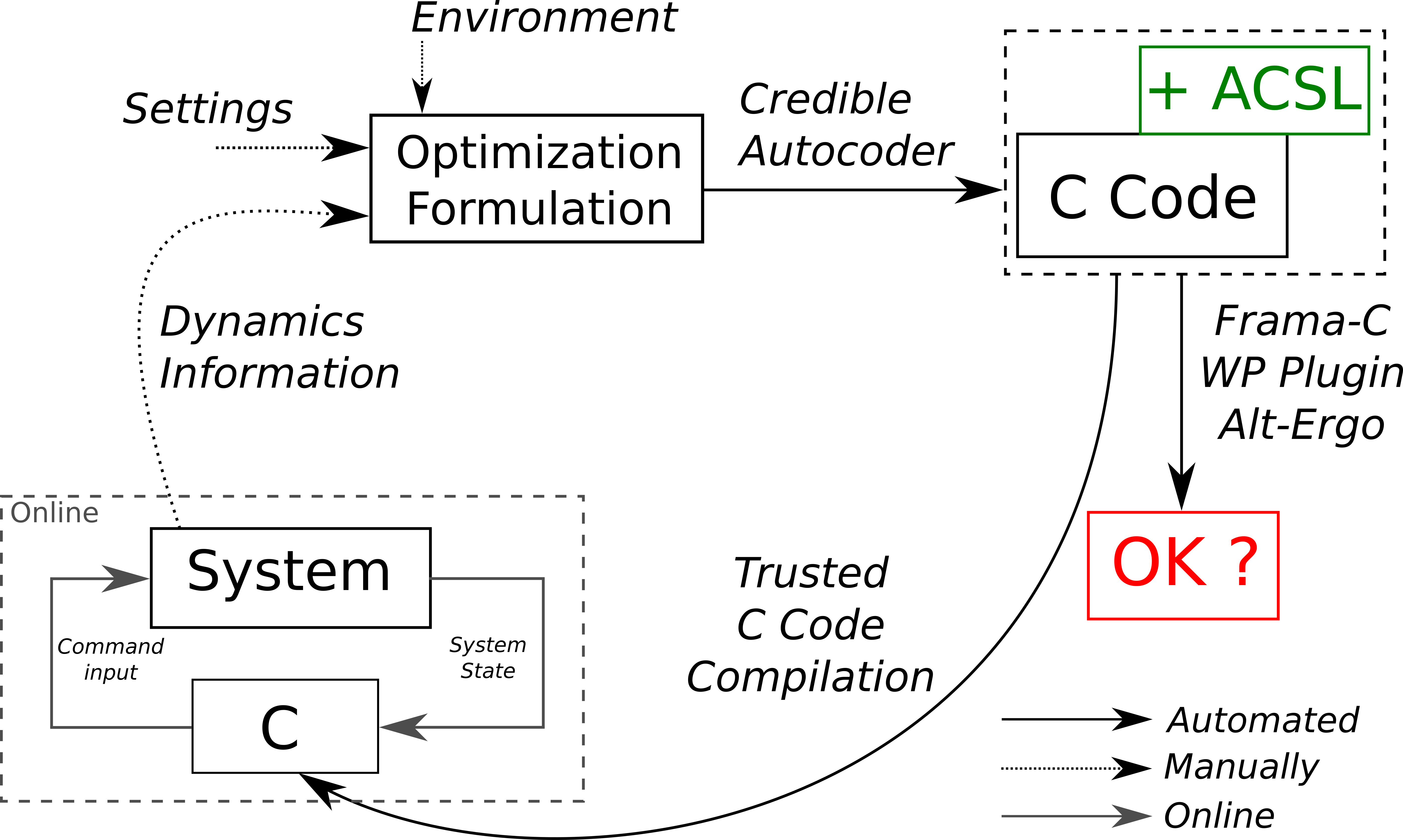
Nevertheless, given that the input text file is written in a high-level language, specifically designed for MPC formulations, it is relatively simple to read. The use of autocoders for automated MPC code generation makes the formulation easier to check and add traceability to the algorithms.
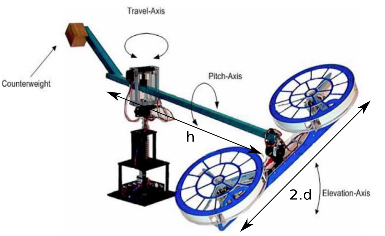
7.2 Example: the three degree-of-freedom helicopter
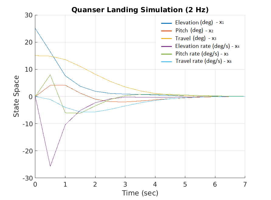
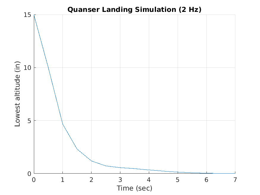
The three degree-of-freedom (3 DOF) helicopter shown in Fig. 17 was used to illustrate the framework developed in this article. The vector state of the system collects the 3 axis angles and rates and it is denoted by . The inputs are the voltages of the front and back DC motors. Further information about the 3 DOF helicopter can be found in [33]. Given an inner feedback controller and a discretization step of , the resulting system is a stable linear system. The problem we are trying to solve is a landing of the 3 DOF helicopter. Starting with an angle of in elevation, in travel (see Fig. 17 for axis) and all the other states being zero, the objective is to design a controller that can drive the system back to the origin while avoiding the ground. The ground is the area below . Thus, the constraint for enforcing ground avoidance is a formula on the elevation and the pitch angles and can be formulated as: . By linearizing this constraint over small angles, one can obtain linear inequalities of the form: . We want to implement the following MPC controller.
| (44) | ||||||
Assuming that , we found, using the method developed in Section 4 a radius (running an off-line optimization problem that finds the largest ball inside ). Similarly, , was obtained using Eq. (28). From the problem formulation, one can see that the norms of the successive ’s along the trajectory constructed are supposed to be minimized. Given a starting point, an upper bound on the objective function over the feasible set can be computed. The objective function is maximal when has the largest norm, and when the system stays at this point throughout the trajectory. The constant can therefore be computed as:
| (45) |
Following those calculations, a number of step of is found. In order to control floating-point errors, a widening coefficient can be constructed. Performing the steps described in Section 6, using double precision floating-points and an accuracy of result in:
As it was explained in Section 6, the ellispoid widening increased the number of iterations needed for the convergence to . The simulation was ran on a Intel Core i5-3450 CPU @ 3.10GHz 4 processor and the running time was approximately for a single point. The results of the simulation can be found in Fig. 18(a) and 18(b). Figure 18(a) presents the closed-loop response for the state vector and Fig. 18(b) shows the lowest altitude point with time for the same simulation. The text file presented in Fig. 19 has been used to generate the C code in order to perform the simulation. The whole simulation was executed using the autocoded C code and a Simulink model. The full autocoder source code, input file (Fig. 19), Simulink model and a user guide for the autocoder can be found online444The source code for the autocoder is available at: https://cavale.enseeiht.fr/quanser_mpc/.
8 Conclusion
In this article, we presented a formal framework for the automatic
generation and verification of optimization code for solving
second-order cone programs. We focused on the ellipsoid method due to
its good numerical characteristics.
We built a framework capable of compiling the high-level requirements
of online receding horizon solvers into C code programs which can then be
automatically verified using existing formal methods tools.
The credible autocoding framework developed is targeting a certain type of
convex optimization problems and the high-level requirements formalized are
appropriately chosen. However, if additional high-level requirements
are needed, some manual
formalization are needed. Although high-level requirements
formalization can be complex,
the struggle during this task is to formalize the low-level mathematical
types and predicates needed.
Hence, this task being already done, the same mathematical foundations can be used and
the formalization of additional high-level requirements
within the credible autocoder is highly simplified.
A numerical analysis of the method has been presented, showing
how to propagate the errors due to floating-point calculations
through the operations performed by the program. A modified version
of the algorithm was presented, allowing us to compute \sayreasonable
a priori bounds on floating-points errors.
However, the numerical analysis performed remains for now purely manual.
Its correctness depends on the exactitude of equations obtained manually
and no verification tools was used for this part. Future work shall
include the use of formal methods to validate the numerical analysis.
Acknowledgments
This work was partially supported by projects ANR ASTRID VORACE, ANR FEANICSES ANR-17-CE25-0018, and NSF CPS SORTIES under grant 1446758. The authors would also like to thank Pierre Roux from ONERA for reviewing this work, and Arkadi Nemirovski for sharing how the Ellipsoid method can be modified to keep the ellipsoid’s condition number bounded.
References
- Jerez et al. [2014] Jerez, J. L., Goulart, P. J., Richter, S., Constantinides, G. A., Kerrigan, E. C., and Morari, M., “Embedded Online Optimization for Model Predictive Control at Megahertz Rates,” IEEE Trans. Automat. Contr., Vol. 59, No. 12, 2014, pp. 3238–3251. 10.1109/TAC.2014.2351991, URL http://dx.doi.org/10.1109/TAC.2014.2351991.
- Açikmese et al. [2013] Açikmese, B., III, J. M. C., and Blackmore, L., “Lossless Convexification of Nonconvex Control Bound and Pointing Constraints of the Soft Landing Optimal Control Problem,” IEEE Trans. Contr. Sys. Techn., Vol. 21, No. 6, 2013, pp. 2104–2113. 10.1109/TCST.2012.2237346, URL http://dx.doi.org/10.1109/TCST.2012.2237346.
- Blackmore [2016] Blackmore, L., The Bridge, Liveright New York, 2016. URL https://www.nae.edu/File.aspx?id=164381.
- Boyd and Vandenberghe [2004] Boyd, S., and Vandenberghe, L., Convex optimization, Cambridge University Press, New York, NY, USA, 2004.
- Mattingley and Boyd [2012] Mattingley, J., and Boyd, S., “CVXGEN: A code generator for embedded convex optimization,” Optimization and Engineering, Vol. 13, No. 1, 2012, pp. 1–27.
- Patrinos et al. [2015] Patrinos, P., Guiggiani, A., and Bemporad, A., “A dual gradient-projection algorithm for model predictive control in fixed-point arithmetic,” Automatica, Vol. 55, 2015, pp. 226–235.
- Feron [2010] Feron, E., “From Control Systems to Control Software,” Control Systems, IEEE, Vol. 30, No. 6, 2010, pp. 50 –71. 10.1109/MCS.2010.938196.
- Champion et al. [2013] Champion, A., Delmas, R., Dierkes, M., Garoche, P.-L., Jobredeaux, R., and Roux, P., “Formal methods for the analysis of critical control systems models: Combining non-linear and linear analyses,” International Workshop on Formal Methods for Industrial Critical Systems, Springer, 2013, pp. 1–16.
- Herencia-Zapana et al. [2012] Herencia-Zapana, H., Jobredeaux, R., Owre, S., Garoche, P.-L., Feron, E., Perez, G., and Ascariz, P., “PVS linear algebra libraries for verification of control software algorithms in C/ACSL,” NASA Formal Methods Symposium, Springer, 2012, pp. 147–161.
- Roux et al. [2012] Roux, P., Jobredeaux, R., Garoche, P.-L., and Féron, É., “A generic ellipsoid abstract domain for linear time invariant systems,” Proceedings of the 15th ACM international conference on Hybrid Systems: Computation and Control, ACM, 2012, pp. 105–114.
- Wang et al. [2016] Wang, T., Jobredeaux, R., Pantel, M., Garoche, P.-L., Feron, E., and Henrion, D., “Credible autocoding of convex optimization algorithms,” Optimization and Engineering, Vol. 17, No. 4, 2016, pp. 781–812.
- Wei [2006] Wei, H., “Numerical stability in linear programming and semidefinite programming,” 2006.
- Cohen et al. [2017] Cohen, R., Davy, G., Feron, E., and Garoche, P.-L., “Formal Verification for Embedded Implementation of Convex Optimization Algorithms,” IFAC-PapersOnLine, Vol. 50, No. 1, 2017, pp. 5867–5874.
- Blackmore et al. [2010] Blackmore, L., Acikmese, B., and Scharf, D. P., “Minimum-landing-error powered-descent guidance for Mars landing using convex optimization,” Journal of guidance, control, and dynamics, Vol. 33, No. 4, 2010, pp. 1161–1171.
- Borrelli et al. [2005] Borrelli, F., Falcone, P., Keviczky, T., Asgari, J., and Hrovat, D., “MPC-based approach to active steering for autonomous vehicle systems,” International Journal of Vehicle Autonomous Systems, Vol. 3, No. 2, 2005, pp. 265–291.
- Floyd [1967] Floyd, R. W., “Assigning Meanings to Programs,” Proceedings of Symposium on Applied Mathematics, Vol. 19, 1967, pp. 19–32.
- Hoare [1969] Hoare, C. A. R., “An axiomatic basis for computer programming,” Commun. ACM, Vol. 12, 1969, pp. 576–580.
- Cuoq et al. [2012] Cuoq, P., Kirchner, F., Kosmatov, N., Prevosto, V., Signoles, J., and Yakobowski, B., “Frama-C: a software analysis perspective,” Springer, 2012, pp. 233–247.
- Baudin et al. [2016] Baudin, P., Filliâtre, J.-C., Marché, C., Monate, B., Moy, Y., and Prevosto, V., “ACSL: ANSI/ISO C Specification Language. Version 1.11.” http://frama-c.com/download/acsl.pdf, 2016.
- Conchon et al. [2012] Conchon, S., Contejean, E., and Iguernelala, M., “Canonized Rewriting and Ground AC Completion Modulo Shostak Theories : Design and Implementation,” Logical Methods in Computer Science, Vol. 8, No. 3, 2012.
- Frama-C [2019] Frama-C, 2019. URL https://frama-c.com/wp.html.
- Grötschel et al. [1981] Grötschel, M., Lovász, L., and Schrijver, A., “The ellipsoid method and its consequences in combinatorial optimization,” Combinatorica, Vol. 1, No. 2, 1981, pp. 169–197.
- Bland et al. [1981] Bland, R. G., Goldfarb, D., and Todd, M. J., “The ellipsoid method: A survey,” Operations research, Vol. 29, No. 6, 1981, pp. 1039–1091.
- Nemirovski [2012] Nemirovski, A., Introduction to Linear Optimization, Lecture notes, Georgia Institute of Technology, 2012.
- Boyd and Barratt [1991] Boyd, S. P., and Barratt, C. H., Linear controller design: limits of performance, Prentice Hall Englewood Cliffs, NJ, 1991.
- Khachiyan [1980] Khachiyan, L. G., “Polynomial algorithms in linear programming,” USSR Computational Mathematics and Mathematical Physics, Vol. 20, No. 1, 1980, pp. 53–72.
- Rump [2006] Rump, S. M., “Verification of positive definiteness,” BIT Numerical Mathematics, Vol. 46, No. 2, 2006, pp. 433–452.
- Rump [2012] Rump, S. M., “Error estimation of floating-point summation and dot product,” BIT Numerical Mathematics, Vol. 52, No. 1, 2012, pp. 201–220.
- Roux et al. [2015] Roux, P., Jobredeaux, R., and Garoche, P., “Closed loop analysis of control command software,” Proceedings of the 18th International Conference on Hybrid Systems: Computation and Control, HSCC’15, Seattle, WA, USA, April 14-16, 2015, 2015, pp. 108–117. 10.1145/2728606.2728623, URL http://doi.acm.org/10.1145/2728606.2728623.
- Goubault and Putot [2011] Goubault, E., and Putot, S., Static Analysis of Finite Precision Computations, Springer Berlin Heidelberg, Berlin, Heidelberg, 2011, pp. 232–247. 10.1007/978-3-642-18275-4_17, URL https://doi.org/10.1007/978-3-642-18275-4_17.
- Putot et al. [2004] Putot, S., Goubault, E., and Martel, M., Static Analysis-Based Validation of Floating-Point Computations, Springer Berlin Heidelberg, Berlin, Heidelberg, 2004, pp. 306–313. 10.1007/978-3-540-24738-8_18, URL https://doi.org/10.1007/978-3-540-24738-8_18.
- El Ghaoui [2002] El Ghaoui, L., “Inversion error, condition number, and approximate inverse of structured matrices,” Linear Algebra and its Applications, Vol. 342, No. 1–3, 2002.
- Quanser [n.d.] Quanser, “3-DOF Helicopter Reference Manual,” , n.d. URL https://www.lehigh.edu/~inconsy/lab/frames/experiments/QUANSER-3DOFHelicopter_Reference_Manual.pdf.