Motion by curvature and large deviations for an interface dynamics on $\mathbb{Z}^{2}$

Abstract: We study large deviations for a Markov process on curves in $\mathbb{Z}^{2}$ mimicking the motion of an interface. Our dynamics can be tuned with a parameter $\beta$, which plays the role of an inverse temperature, and coincides at $\beta=\infty$ with the zero-temperature Ising model Glauber dynamics, where curves correspond to the boundaries of droplets of one phase immersed in a sea of the other one. The diffusion coefficient and mobility of the model are identified and correspond to those predicted in the literature. We prove that contours typically follow a motion by curvature with an influence of the parameter $\beta$, and establish large deviation bounds at all large enough $\beta<\infty$.

1 Introduction

A basic paradigm in non-equilibrium statistical mechanics is the following. Consider a system with two coexisting pure phases separated by an interface, and undergoing a first-order phase transition with non-conserved order parameter. Then, macroscopically, the interface should evolve in time to reduce its surface tension, according to a motion by curvature. For microscopic models on a lattice, some trace of the lattice symmetries should remain at the macroscopic scale, and the resulting motion by curvature should be anisotropic. The following general behaviour, known as the Lifshitz law, is expected: if a droplet of linear size $N\gg 1$ of one phase is immersed in a sea of the other phase, then it should disappear in a time of order $N^{2}$. (Anisotropic) motion by curvature should correspond to the limiting dynamics, when $N$ is large, under diffusive rescaling of space and time. Phenomenological arguments in favour of this picture go back to Lifshitz [Lif62], and can be summarised as follows. Consider a model with surface tension $\mathfrak{t}=\mathfrak{t}({\bf N})$, which depends on the local inwards normal ${\bf N}$ to an interface. We work in two dimensions to keep things simple. The surface energy associated with a curve $\gamma$ separating two phases reads:

$$F(\gamma)=\int_{\gamma}\mathfrak{t}({\bf N}(s))ds,$$ (1.1)

where $s$ is the arclength coordinate on $\gamma$. The postulate, on phenomenological grounds, is that the local inwards normal speed $v$ to the interface reads

$$v=\mu\frac{\delta F}{\delta\gamma}.$$ (1.2)

Above, $\delta F/\delta\gamma$ is the variational derivative of $F$, defined informally below. The quantity $\mu=\mu({\bf N})$ is the mobility of the model, computed by Spohn in [Spo93] using linear response arguments. Let us relate (1.2) and motion by curvature. The change $\delta F=\delta F({\bf N})$ in energy induced by the motion of a length $ds$ in the normal direction ${\bf N}$ is equal to $(\mathfrak{t}({\bf N})/R({\bf N}))ds$, which can be written $\delta F/\delta\gamma=\mathfrak{t}({\bf N})/R({\bf N})$, with $R({\bf N})$ the radius of curvature at ${\bf N}$. As such:

$$v=\mu\mathfrak{t}k=:ak,\quad\text{ with }\quad a({\bf N})=\mu({\bf N})\mathfrak{t}({\bf N})\text{ the anisotropy and }k=1/R\text{ the curvature}.$$ (1.3)

A closed curve satisfying (1.3) is said to evolve according to anisotropic motion by curvature. A set with boundary following this equation is known to shrink to a point in finite time for a wide range of anisotropies $a$, see e.g. [LST14] and references therein.

Ideally, one would like to start from a microscopic model with short-range interactions, with at least two different phases initially segregated on a macroscopic scale, and derive motion by curvature (1.3) of the boundaries between the phases in the diffusive scaling. To this day however, results on microscopic models are scarce. Let us provide a (non-exhaustive) account of works on the subject.
The paper [Spo93], already cited, is a landmark in the rigorous study of interface motion starting from microscopic models. A major difficulty is to understand how to decouple, from the comparatively slower motion of the interface, the fast relaxation inside the bulk of each phase. Indeed, in a diffusive time scale and at least for models with local interactions, one expects the bulk to behave as if at equilibrium.
In models where the interface is the graph of a function of a one-dimensional parameter, motion by curvature has been proven for a number of interacting particle systems. Motion by curvature usually boils down to the heat equation in this case, and the Lifshitz law is related to freezing/melting problems, see [CS96][CK08][CKG12], as well as [Lac14] and the monograph [Car+16].
For one-dimensional interfaces in two dimensions, a landmark is the proof of anisotropic motion by curvature for the Glauber dynamics of the zero temperature Ising model (henceforth zero-temperature Ising dynamics). The drift of the interface at time $0$ was computed in [CL07] for several types of initial conditions, before the full motion by curvature (1.3) was proven in [LST14a]-[LST14]. Their proof crucially relies on monotonicity of the Glauber dynamics.
More is known on another type of microscopic models for which some sort of a mean-field mesoscopic description can be achieved. This comprises the so-called Glauber+Kawasaki process [DFL86] (see also [BBP18] for an account of works on the model), which has local evolution rules, and models with long range interactions such as the Ising model with Kac potentials [Com87][De ̵+93][De ̵+94][KS94]. For these models, studied in any dimension, the derivation takes place in two steps: first deriving a mean-field description of the dynamics, then rescaling space-time to derive motion by curvature. As a result, lattice symmetries are blurred and the resulting motion by curvature is isotropic. Note however the recent works [FT19][Ket+20], where a Glauber+Kawasaki dynamics is considered (respectively Glauber+Zero-range), in dimension two and above. In these works, the existence of an interface between regions at high- and low-density is established, and motion by curvature for this interface is obtained directly from the microscopic model, in a suitable scaling of the Glauber part of the dynamics.
A last category of models comprises the so-called effective interface models. In these models, an interface between phases is represented by the graph of a given function, with which an "interfacial" cost is associated. Only the interface is relevant, and the phases it separates are not described. Effective interface models comprise the Ginzburg-Landau model in any dimension, see [FS97], and more recently Lozenge-tiling dynamics in dimension three [LT18].

To better understand the structure of interface dynamics, another related line of investigation concerns large deviations of the motion of an interface around motion by curvature. Assuming Gaussian-like fluctuations around the mean behaviour (1.3), the rate function describing the cost of observing an abnormal trajectory $\gamma_{\cdot}=(\gamma_{t})_{t\leq T}$ should read:

$$I(\gamma_{\cdot})=\int_{0}^{T}dt\int_{\gamma_{t}}\frac{(v-ak)^{2}}{2\mu}ds,$$ (1.4)

with $s$ the arclength coordinate on $\gamma_{t}$. In the assumption of Gaussian fluctuations leading to (1.4), one of the difficulties is that it is not even clear how the noise should be incorporated into the deterministic equations describing the interface motion. Extensive work on this question has been carried out for some of the models listed above in recent years, notably in [BBP17]-[BBP18] (see also the references there). In [BBP17], the stochastic Allen-Cahn equation is considered. It is known that, in the diffusive (or sharp interface) limit, solutions to the Allen-Cahn equation satisfy motion by mean curvature in some sense, see [Ilm93] [ESS92] [BSS93]. In [BBP17a], regularity of solutions to the stochastic Allen-Cahn equation depending on how the noise is added are studied, and a large deviation upper-bound in the joint diffusive, small noise and vanishing regularisation limits is established in [BBP17]. The associated rate function coincides with (1.4) in simple cases, e.g. for a droplet trajectory with smooth boundary. The authors however use tools from geometric measure theory, which enable them to consider very general trajectories that may feature nucleation events.
In [BBP18], upper bound large deviations for both Glauber+Kawasaki process and Ising model with Kac potentials are investigated. They prove that (1.4) is the correct rate function for smooth trajectories and discuss how to extend it to more general paths.

To the best of our knowledge however, no results on large deviations from motion by curvature for microscopic interface dynamics with local interactions have yet been published. In particular the question of large deviations for the zero temperature Ising Glauber dynamics is still open.
In this work, we present a family of interface dynamics, that we call the contour dynamics. This dynamics typically evolves by motion by curvature, and we characterise the large deviations. It is closely related to the zero temperature Glauber dynamics for the Ising model: the contour dynamics has the same updates, except that additional moves depending on a parameter $\beta>0$ are allowed. This parameter $\beta$ plays the role of an inverse temperature acting on local portions of the contours. The model at each $\beta>0$ has reversible dynamics and, contrary to the Glauber dynamics for the zero temperature Ising model, the dynamics is not monotonous. When $\beta=\infty$, the update rules of the contour dynamics are exactly the same as the Ising ones. Large deviations for the contour dynamics are studied using the method initiated by Kipnis, Olla and Varadhan in [KOV89] (see also Chapter 10 in [KL99]). There are substantial difficulties as we are dealing with curves, i.e. one-dimensional objects, evolving in two-dimensional space. One of the advantages of the method is that we no longer rely on monotonicity of the dynamics as in [LST14]. Monotonicity appears difficult to use for large deviations in any case, as atypical events, such as closeness to some atypical trajectory, are in general not monotonous. At each large enough $\beta>0$, we prove that the dynamics approaches anisotropic motion by curvature in the large size limit, with a dependence on the parameter $\beta$. At the formal level, the $\beta=\infty$ case indeed corresponds to anisotropic motion by curvature in the sense of [LST14a]. We then obtain large deviations for the model, with a rate function that agrees with (1.4) for sufficiently nice trajectories.

The rest of this article is structured as follows. In Section 2, we introduce the microscopic model and fix notations. The dynamics is introduced in details using the stochastic Ising dynamics as comparison, while useful topological facts are collected in Appendix B. The main results of the paper are listed in Section 2, with Section 2.4 presenting the structure of the proof as well as a connection of the contour dynamics with the exclusion process, a guideline of the paper.
In Section 3, following the large deviation approach of [KOV89], we compute Radon-Nikodym derivatives for a large class of tilted dynamics. Under the assumption that trajectories live in a nice enough space, we show how motion by curvature emerges from the microscopic computations as well as the influence of the parameter $\beta$. The computations of the Radon-Nikodym derivative are then used to prove large deviations, with the upper bound in Section 4 and the lower bound in Section 5. A number of technical results and sub-exponential estimates are postponed to Section 6 and Appendices A-B. In particular, Section 6 is a collection of estimates that are genuinely particular to our model, concerning the dynamical behaviour of the poles, i.e. the sections of the contours on which the parameter $\beta$ acts.

2 Model and results

2.1 Zero temperature Glauber dynamics for the Ising model

The contour dynamics studied in this paper is closely related to the Glauber dynamics of the zero temperature, two-dimensional Ising model on $(\mathbb{Z}^{*})^{2}$ (henceforth zero temperature Glauber dynamics), with $\mathbb{Z}^{*}:=\mathbb{Z}+1/2$ the dual graph of $\mathbb{Z}$. Looking at $(\mathbb{Z}^{*})^{2}$ rather than $\mathbb{Z}^{2}$ is meant to ensure that contours are lattice paths on $\mathbb{Z}^{2}$, see below. Let us first define this Markov process.
On the space $\Sigma:=\{-1,1\}^{(\mathbb{Z}^{*})^{2}}$ of all spin configurations $\sigma=(\sigma(i))_{i\in(\mathbb{Z}^{*})^{2}}\in\Sigma$, define the dynamics as follows: each site $i\in(\mathbb{Z}^{*})^{2}$ is updated independently at rate $1$. The spin $\sigma(i)$ at site $i$ takes the same value as the majority of its neighbours, where spins $\sigma(j),\sigma(k)$ are neighbours for $j,k\in(\mathbb{Z}^{*})^{2}$ if $\|j-k\|_{1}=1$. If spin $\sigma(i)$ has exactly two neighbours of each sign, then with probability $1/2$ $\sigma(i)$ remains unchanged, and with probability $1/2$ it is flipped, i.e. changed to $-\sigma(i)$. A spin with three or more neighbours of the same sign is not changed, while a spin with three or more neighbours of opposite sign is flipped instantaneously, and the process is repeated until no such spin remains. This is summarised in the following jump rates (see also Figure 1): for each configuration $\sigma$ and each $i\in(\mathbb{Z}^{*})^{2}$,

$$c(\sigma,\sigma^{i})=\begin{cases}0\quad&\text{if }\sigma(i)\text{ and at least three neighbours have the same sign},\\ 1/2\quad&\text{if }\sigma(i)\text{ has two neighbours of each sign},\\ +\infty\quad&\text{if }\sigma(i)\text{ has at least three neighbours with opposite sign}.\end{cases}$$ (2.1)

Above, the configuration $\sigma^{i}$ is the same as $\sigma$, except that the spin at $i$ has been flipped:

$$\forall j\in(\mathbb{Z}^{*})^{2}\setminus\{i\},\qquad\sigma^{i}(j)=\sigma(j),\qquad\sigma^{i}(i)=-\sigma(i).$$ (2.2)

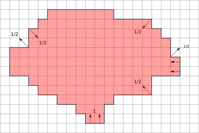
Figure 1: Some possible updates in the Glauber dynamics for the zero temperature stochastic Ising dynamics. Red squares represent $-$ spins, white squares $+$ spins, assimilating a square with its centre, a point of $(\mathbb{Z}^{*})^{2}$. If either of the lowest two red squares disappear (at rate 1/2, since both have two neighbours of each colour), then the other one has three neighbours of opposite colour and is flipped instantaneously. Both these squares thus become white at rate $1$. After that move, the Glauber rules preclude any square of the line from becoming red. In particular, the zero temperature Ising dynamics is irreversible.

Rather than spins, the zero temperature Glauber dynamics can alternatively be defined in terms of blocks: a block is a subset of $\mathbb{R}^{2}$ of the form $i+[-1/2,1/2]^{2}$, with $i\in(\mathbb{Z}^{*})^{2}$ the centre of the block. Flipping a spin amounts to changing the colour of the corresponding block. The colour of a block (red or white in Figure 1) is determined by the sign of the spin at its centre. This alternative terminology will be used preferentially throughout the article. In fact, we will consider configurations of the type depicted in Figure 1, where all red blocks form a bounded connected region (that we call a droplet, see next paragraph) surrounded by white blocks. We will then not even focus on colours, and instead say that a block is added/deleted to mean that the new droplet contains one more/one less block.

In [LST14a]-[LST14], the evolution of a droplet of $-$ spins surrounded by $+$ spins is studied for a slightly different choice of jump rates (but the result applies to the present case (2.1)). Let us describe their result. Let $\gamma^{0}\subset\mathbb{R}^{2}$ be a Jordan curve, i.e. a closed, simple curve. Let $\Gamma^{0}$ be the droplet associated with $\gamma^{0}$, meaning the compact subset of $\mathbb{R}^{2}$ with boundary $\partial\Gamma^{0}=\gamma^{0}$. Assume for simplicity that $\Gamma^{0}$ is convex and $\gamma^{0}$ is $C^{\infty}$ (the non-convex case is treated in [LST14]). Fix a scaling parameter $N\in\mathbb{N}^{*}$, and let $\sigma^{0}\in\Sigma$ be the spin configuration obtained by setting $\sigma^{0}(i)=-1$ if $i\in N\Gamma^{0}$, $\sigma^{0}(i)=1$ if $i\notin N\Gamma^{0}$. For convenience, we may assume, up to adding a finite number of $-$ spins, that each $-$ spin in $\sigma^{0}$ has at least two $-$ neighbours as in Figure 1. The zero temperature Glauber dynamics (2.1) starting from $\sigma^{0}$ is then well defined for all time.

In [LST14a], the authors prove that, rescaling space by $1/N$ and time by $N^{2}$, the rescaled droplet converges uniformly in time and in Hausdorff distance to the unique solution of an anisotropic motion by curvature starting from $\Gamma^{0}$. To state a precise result, we need some notation. A solution $(\Gamma_{t})_{t\geq 0}$ of motion by curvature (1.3) with initial condition $\Gamma^{0}$ is a flow of droplets starting at $\Gamma^{0}$ and satisfying the following: there is a time $T_{f}>0$ such that, for $t<T_{f}$, the boundaries $(\gamma_{t})_{t<T_{f}}$ of $(\Gamma_{t})_{t<T_{f}}$, parametrised on the unit torus $\mathbb{T}$, solve (1.3):

$$\forall u\in\mathbb{T},\forall t<T_{f},\qquad\partial_{t}\gamma_{t}(u)=a(\theta(t,u))\partial^{2}_{s}\gamma(t,u)=a(\theta(t,u))k(t,u){\bf N}(t,u).$$ (2.3)

Moreover, after time $T_{f}$, each droplet $\Gamma_{t}$ is reduced to a point. In (2.3), the letter $s$ denotes the arclength coordinate on the curve $\gamma_{t}$ for $t<T_{f}$, while $k(t,u)$ is the curvature, and $\theta(t,u)$ is the angle between the tangent vector at point $\gamma_{t}(u)$ and the first basis vector ${\bf b}_{1}:=(1,0)$. The vector ${\bf N}(t,u)$ is the unit inwards normal at $\gamma_{t}(u)$. The $\pi/2$-periodic anisotropy factor $a$ is a quantity with symmetries reflecting those of the square lattice. It reads:

$$a(\theta):=\frac{1}{2(|\sin(\theta)|+|\cos(\theta)|)^{2}},\qquad\theta\in[0,2\pi].$$ (2.4)

Existence and uniqueness of a flow of sets solving (2.3) is part of the results of [LST14a]-[LST14].
For a set $\Gamma\subset\mathbb{R}^{2}$ and $\varepsilon>0$, let $\Gamma^{(-\varepsilon)}$ (resp.: $\Gamma^{(\varepsilon)}$) denote its $\varepsilon$-shrinking (resp.: $\varepsilon$-fattening):

$$\Gamma^{(\varepsilon)}=\bigcup_{x\in\Gamma}B_{1}(x,\varepsilon),\qquad\Gamma^{(-\varepsilon)}=\Big{[}\bigcup_{x\notin\Gamma}B_{1}(x,\varepsilon)\Big{]}^{c},$$ (2.5)

where $B_{1}(x,\varepsilon)$ is the ball of centre $x$ and radius $\varepsilon$ in $1$-norm. For future reference, recall:

$$\forall(u,v)\in\mathbb{R}^{2},\qquad\|(u,v)\|_{1}:=|u|+|v|,\quad\|(u,v)\|_{2}=\sqrt{u^{2}+v^{2}},\quad\|(u,v)\|_{\infty}=\max\{|u|,|v|\}.$$ (2.6)

The main result of [LST14a] is then the following. Denote as before by $(\Gamma_{t})_{t\geq 0}$ the flow of droplets satisfying (2.3) with initial condition $\Gamma^{0}$. Let $\mathbb{P}$ denote the probability associated with the zero temperature Glauber dynamics starting from the configuration $\sigma^{0}$, and let $\Gamma^{N}$ be the notation for a microscopic droplet of $-$ spins. Then the rescaled droplet trajectory evolves in diffusive time and satisfies (2.3), in the sense that:

$$\forall\varepsilon>0,\qquad\lim_{N\rightarrow\infty}\mathbb{P}\Big{(}\forall t\geq 0,\quad\Gamma_{t}^{(-\varepsilon)}\subset N^{-1}\Gamma^{N}_{tN^{2}}\subset\Gamma_{t}^{(\varepsilon)}\Big{)}=1,$$ (2.7)

and:

$$\forall\varepsilon>0,\qquad\lim_{N\rightarrow\infty}\mathbb{P}\Big{(}\forall t\geq T_{f}+\varepsilon,\quad\Gamma^{N}(tN^{2})=\emptyset\Big{)}=1.$$ (2.8)

For future reference, note that (2.7) is a statement on the Hausdorff distance $d_{\mathcal{H}}$ of $N^{-1}\Gamma^{N}_{tN^{2}}$ and $\Gamma_{t}$ at each time $t\geq 0$. The Hausdorff distance between two non-empty, compact sets $A,B\subset\mathbb{R}^{2}$ reads:

$$d_{\mathcal{H}}(A,B)=\inf\big{\{}\varepsilon>0:A\subset B^{(\varepsilon)}\text{ and }B\subset A^{(\varepsilon)}\big{\}}.$$ (2.9)

The proof of (2.7)-(2.8) relies strongly on two ingredients. The first ingredient is the fact that the zero temperature Glauber dynamics has the monotonicity property (see e.g. Section 3.3 in [Mar99]): for two spin configurations $\sigma,\eta$, write $\sigma\leq\eta$ when $\sigma_{i}\leq\eta_{i}$ for each $i\in(\mathbb{Z}^{*})^{2}$. There is then a coupling such that, with probability $1$, $\sigma_{t}\leq\eta_{t}$ for all $t\geq 0$.
The second ingredient is the observation that local portions of the interface can be mapped to one-dimensional interacting particle processes, in particular to the symmetric simple exclusion process (SSEP), which is well known. This mapping is detailed in Section 2.4.

2.2 The contour dynamics

In this article, we consider a microscopic interface dynamics that we call the contour dynamics. It is closely related to the zero-temperature Glauber dynamics, but presents a number of interesting contrasting features. In this section, we first describe the state space, then define the dynamics. A connection of the contour dynamics with the simple exclusion process is then presented, and further elaborated on in Section 2.4. This connection will serve as a guideline throughout the article.

2.2.1 The state space

Before defining the contour dynamics, let us present what kind of interfaces will be considered. Take a Lipschitz Jordan curve $\gamma\subset\mathbb{R}^{2}$, and denote by $\Gamma\subset\mathbb{R}^{2}$ the droplet associated with $\gamma$, defined as the compact set with boundary $\partial\Gamma=\gamma$. A typical situation where the evolution of the interfaces under the Ising dynamics is known [LST14a] is the case where the starting droplet $\Gamma$ is convex (and $\gamma$ is smooth enough). In this case, the trajectory $(\gamma_{t})_{t\geq 0}$ of interfaces solving (2.3) starting from $\gamma$ is associated with convex droplets. At the microscopic level, convexity is however not a useful notion. To see it, let $\Gamma^{N}$ be the droplet of $-$ spins with associated blocks included in $N\Gamma$. Then $\Gamma^{N}$ is in general not convex, nor is convexity preserved in general by a spin flip with the rules (2.1) (see Figure 1).
However, like $\gamma$, the boundary $\gamma^{N}:=\partial\Gamma^{N}$ of the microscopic droplet has Property 2.1 below. To state it, define first, for $\theta\in[0,2\pi]$ the vectors ${\bf b}_{\theta}$, ${\bf b}_{1},{\bf b}_{2}$ as:

$${\bf b}_{\theta}:=\cos(\theta){\bf b}_{1}+\sin(\theta){\bf b}_{2},\qquad{\bf b}_{1}=(1,0)={\bf b}_{\theta=0},\quad{\bf b}_{2}=(0,1)={\bf b}_{\theta=\pi/2}.$$ (2.10)

By convention, interfaces in this article are oriented clockwise.
Both $\gamma^{N}$ and $\gamma$ are Lipschitz curves, so their tangent vector ${\bf T}$ is defined at almost every point of the interface. Property 2.1 shared by $\gamma^{N}$ and $\gamma$ is then the following.

Property 2.1.

The interface can be split into four (intersecting) connected regions of maximal length, such that the tangent vector ${\bf T}$ to the interface at each point of region $k$ (with $1\leq k\leq 4$), whenever it is defined, points towards the quarter plane $({\bf b}_{-(k-1)\pi/2},{\bf b}_{-k\pi/2})$ (see Figure 2).

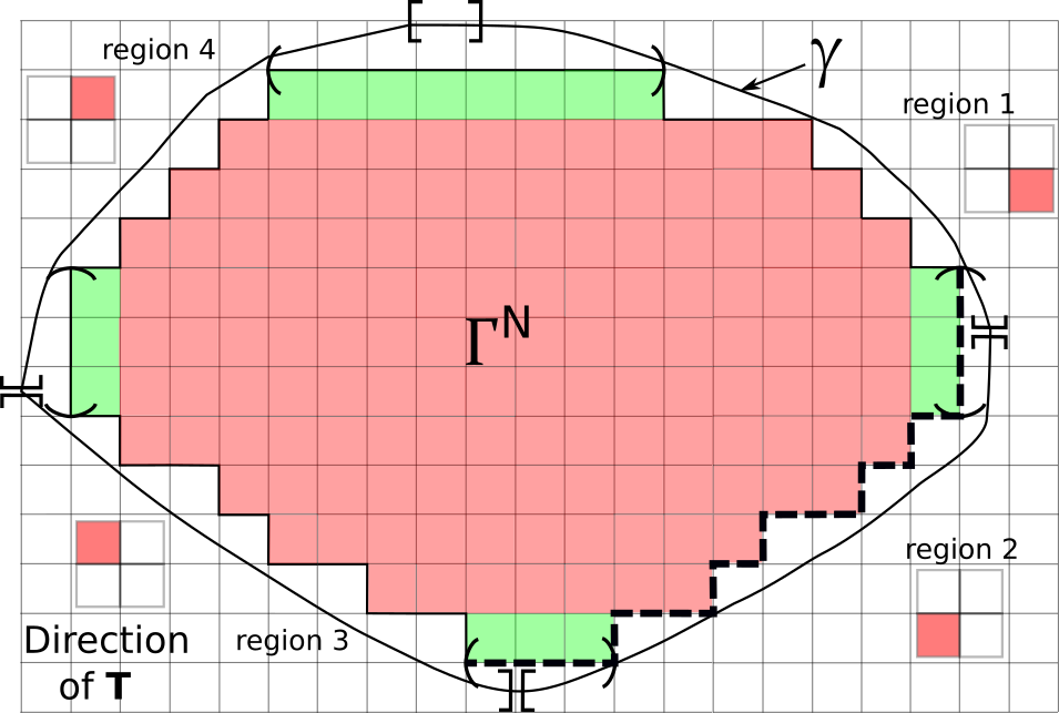
Figure 2: The convex interface $\gamma$ and the droplet $\Gamma^{N}$ associated with the discretisation $\gamma^{N}:=\partial\Gamma^{N}$ of $\gamma$. The four regions of both $\gamma$ and $\gamma^{N}$ are materialised by opening and closing brackets ($\gamma$) or parentheses ($\gamma^{N}$), with each region starting with an opening symbol and ending with a closing one. As an example, region 2 of $\gamma^{N}$ corresponds to the thick dashed lines. The quarterplane to which the tangent vector ${\bf T}$ belongs is indicated as a red square for each region. The regions intersect at the poles. All poles of $\gamma$ are reduced to points except the north pole (pole 1), while poles of $\gamma^{N}$ must contain at least two edges. The spins (i.e. the blocks) which have an edge belonging to a pole are coloured in green.

Note that for a discrete interface, the tangent vector can actually only be one the four vectors ${\bf b}_{k\pi/2}$ ($1\leq k\leq 4$), corresponding to $\pm{\bf b}_{1},\pm{\bf b}_{2}$.
For an interface satisfying Property 2.1, the intervals corresponding to the intersection of two consecutive regions will play a special role. These intervals (see Figure 2) are called poles, and correspond to points of the interface with extremal abscissa or ordinate. Pole $k$ ($1\leq k\leq 4$) is defined as the intersection of regions $k-1$ and $k$, where by convention $k-1:=4$ if $k=1$. We shall also refer to poles in terms of cardinal directions: pole $1$ is the north pole, corresponding to the interval of points with maximal ordinate. Pole $2$ is the east pole, made of points with maximal abscissa, etc.

We can now define the state space of the contour dynamics. In view of the hydrodynamic behaviour (2.7), we directly work with rescaled microscopic curves, i.e. lattice paths on $(N^{-1}\mathbb{Z})^{2}$ ($N$ is the scaling parameter). In the following, an edge of the graph $(N^{-1}\mathbb{Z})^{2}$ is identified with a segment of length $1/N$ between two neighbouring vertices.

Definition 2.2 (State space).

Let $\Omega$ denote the set of Lipschitz, closed curves in $\mathbb{R}^{2}$ satisfying Property 2.1. For an integer $N\in\mathbb{N}^{*}$, the microscopic state space $\Omega^{N}_{\text{mic}}$ is the subset of $\Omega$ such that:

• Each curve $\gamma^{N}\in\Omega^{N}_{\text{mic}}$ is a simple, closed lattice path on $(N^{-1}\mathbb{Z})^{2}$.

• Each of the four poles of $\gamma^{N}$ contains at least two edges, i.e. it is a segment of length at least $2/N$.

• The droplet $\Gamma^{N}$ associated with $\gamma^{N}\in\Omega^{N}_{\text{mic}}$ (i.e. the compact region with boundary $\gamma^{N}$) contains the origin $0\in\mathbb{Z}^{2}$ (see item 2 in Remark 2.4 below).

The intervals that we call poles are going to play an important role, and we now fix some notations. Take a curve $\gamma\in\Omega$ and let $P_{k}=P_{k}(\gamma)$ denote its pole $k$ ($1\leq k\leq 4$). Write $P_{k}=[L_{k},R_{k}]$, where the points $L_{k},R_{k}=L_{k}(\gamma),R_{k}(\gamma)$ of $\mathbb{R}^{2}$ are respectively the left and right extremities of $P_{k}$ when $\gamma$ is oriented clockwise (as will always be the case), see Figure 3 below. The length of pole $k$ is denoted by $|P_{k}|$.
In analogy with the Ising case, if $i\in(N^{-1}\mathbb{Z}^{*})^{2}$, the block $C_{i}$ with centre $i$ is defined as:

$$C_{i}:=i+\frac{1}{2N}[-1,1]^{2}.$$ (2.11)

If $\gamma^{N}\in\Omega^{N}_{\text{mic}}$ is a microscopic curve, we then say that a block in the droplet $\Gamma^{N}$ delimited by $\gamma^{N}$ is in pole $k$ ($1\leq k\leq 4$) if one of the edges of its boundaries is included in pole $k$. Blocks in a pole are those in green on Figure 2. Let $p_{k}=p_{k}(\gamma^{N})$ denote the number of blocks in pole $k$. It is related to the length $|P_{k}|$ of the pole by:

$$p_{k}:=N|P_{k}|,\qquad 1\leq k\leq 4.$$ (2.12)

2.2.2 The dynamics

Let us now define the contour dynamics on $\Omega^{N}_{\text{mic}}$ (see Figure 3). To do so, we first fix some notations. Let $\gamma^{N}\in\Omega^{N}_{\text{mic}}$ and $\Gamma^{N}$ denote the associated droplet as usual. If $i\in(N^{-1}\mathbb{Z}^{*})^{2}$, adding or deleting block $C_{i}:=i+\frac{1}{2N}[-1,1]^{2}$ to $\Gamma^{N}$ amounts to the operation $\Gamma^{N}\rightarrow(\Gamma^{N})^{i}$, with:

$$(\Gamma^{N})^{i}:=\begin{cases}\Gamma^{N}\cup C_{i}\quad&\text{if }i\notin\Gamma^{N},\\ \Gamma^{N}\setminus C_{i}\quad&\text{if }i\in\Gamma^{N}.\end{cases}$$ (2.13)

Define then $(\gamma^{N})^{i}:=\partial\big{(}(\Gamma^{N})^{i}\big{)}$.

Consider now moves affecting the poles. For $k$ with $1\leq k\leq 4$, assume that pole $k$ of $\gamma^{N}$ contains exactly two blocks. Define then $(\gamma^{N})^{-,k}$ as the boundary of $(\Gamma^{N})^{-,k}$, where $(\Gamma^{N})^{-,k}$ is obtained from $\Gamma^{N}$ by deleting the two blocks in pole $k$:

$$(\Gamma^{N})^{-,k}:=\Gamma^{N}\setminus\bigcup_{i\in(N^{-1}\mathbb{Z}^{*})^{2}:C_{i}\text{ is in Pole }k}C_{i}\qquad(\gamma^{N})^{-,k}=\partial\big{(}(\Gamma^{N})^{-,k}\big{)}.$$ (2.14)

Define conversely a transformation that makes a droplet grow at the pole as follows. Let $x\in(N^{-1}\mathbb{Z})^{2}\cap P_{k}$, $1\leq k\leq 4$ be such that $x\notin\{R_{k},L_{k}\}$. Define then $(\gamma^{N})^{+,x}$ as the boundary of $(\Gamma^{N})^{+,x}$, with:

$$(\Gamma^{N})^{+,x}:=\Gamma^{N}\cup\bigcup_{i\in(N^{-1}\mathbb{Z}^{*})^{2}\setminus\Gamma^{N}:x\in C_{i}}C_{i},\qquad(\gamma^{N})^{+,x}=\partial\big{(}(\Gamma^{N})^{+,x}\big{)}.$$ (2.15)

In words, $(\Gamma^{N})^{+,x}$ is the droplet $\Gamma^{N}$ to which the two blocks that contain $x$ and that are not in pole $k$ have been added. We can now define the contour dynamics, illustrated on Figure 3.

Definition 2.3.

The contour dynamics on $\Omega^{N}_{\text{mic}}$ at inverse temperature $\beta>0$ is defined through the jump rates $c(\gamma^{N},\tilde{\gamma}^{N})$ for curves $\gamma^{N},\tilde{\gamma}^{N}\in\Omega^{N}_{\text{mic}}$:

• $c\big{(}\gamma^{N},(\gamma^{N})^{i}\big{)}=(1/2){\bf 1}_{(\gamma^{N})^{i}\in\Omega^{N}_{\text{mic}}}$ for $i\in(N^{-1}\mathbb{Z}^{*})^{2}$;

• $c\big{(}\gamma^{N},(\gamma^{N})^{-,k}\big{)}={\bf 1}_{p_{k}(\gamma^{N})=2}{\bf 1}_{(\gamma^{N})^{-,k}\in\Omega^{N}_{\text{mic}}}$, with $p_{k}$ defined in (2.12) for $1\leq k\leq 4$;

• (Growth at the poles) $c\big{(}\gamma^{N},(\gamma^{N})^{+,x}\big{)}=e^{-2\beta}$ for each $x\in(N^{-1}\mathbb{Z})^{2}\cap P_{k}(\gamma^{N})$ with $x\notin\{R_{k}(\gamma^{N}),L_{k}(\gamma^{N})\}$, $1\leq k\leq 4$;

• $c(\gamma^{N},\tilde{\gamma}^{N})=0$ for any other $\gamma^{N},\tilde{\gamma}^{N}$.

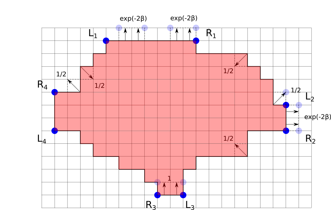
Figure 3: Some moves and associated jump rates for the contour dynamics acting on an element of $\Omega^{N}_{\text{mic}}$. Positions of the extremities $L_{k},R_{k}$, $1\leq k\leq 4$ of the poles are represented by dark dots. Possible positions of $L_{k},R_{k}$ after a jump are represented by light dots. Dynamical moves amount to adding or deleting squares of side-length $1/N$ ("blocks"). The pole $P_{3}$ contains two blocks, i.e. $p_{3}=2$, thus an update deletes both of its blocks simultaneously.

Remark 2.4.

Let us comment on Definition 2.3.

• If $\beta=+\infty$, then the contour dynamics and the zero temperature Glauber dynamics (2.1) act on a contour $\gamma^{N}\in\Omega^{N}_{\text{mic}}$ in the same way, provided the resulting contour is in $\Omega^{N}_{\text{mic}}$.

• At each $\beta>0$, the contour dynamics is not monotonous (see Figure 4). However, it is built to be reversible with respect to the measure $\nu^{N}_{\beta}$, defined by:

  $$\nu^{N}_{\beta}(\gamma):=\frac{1}{\mathcal{Z}^{N}_{\beta}}e^{-\beta N|\gamma^{N}|},\qquad\gamma^{N}\in\Omega^{N}_{\text{mic}},\quad\mathcal{Z}^{N}_{\beta}\text{ a normalisation factor.}$$ (2.16)

  Recall that elements of $\Omega^{N}_{\text{mic}}$ must surround the point $0$ by Definition 2.2. This serves to break translation invariance, so that $\nu^{N}_{\beta}$ is well-defined as soon as $\beta>\log 2$ (the number of curves of length $n/N$ in $\Omega^{N}_{\text{mic}}$ is bounded by $cn^{4}2^{n}$ for some $c>0$ and each $n\in\mathbb{N}$). In fact, all results below are stated for $\beta>1$.
  Reversibility is an important difference from the zero temperature Glauber dynamics (2.1), where regrowth of the droplet was not possible. In addition, the fact that the invariant measure $\nu^{N}_{\beta}$ is sufficiently nice to perform computations is key to the results of this paper, as it allows for the use of the entropy method of Guo, Papanicolaou and Varadhan [GPV88]. Due to the regrowth term in the contour dynamics, one however has to carefully control the motion of the poles, which is the main difficulty of this study at the microscopic level.
  

• The contour dynamics is non-local: one cannot find $\rho\in\mathbb{N}^{*}$ independent of $N$ such that, for any $\gamma^{N}\in\Omega^{N}_{\text{mic}}$ and any $x\in\gamma^{N}\cap(N^{-1}\mathbb{Z})^{2}$, deciding whether $c\big{(}\gamma^{N},(\gamma^{N})^{x}\big{)}>0$ require only the knowledge of all points of the curve at $1$-distance at most $\rho/N$ from $x$. This is due to the fact that regions $1$ and $3$, or $2$ and $4$ of a curve in $\Omega^{N}_{\text{mic}}$ may be very close to each other, so that deleting a single block would create self-intersections in the interface, which is forbidden. This point is illustrated on Figure 4.

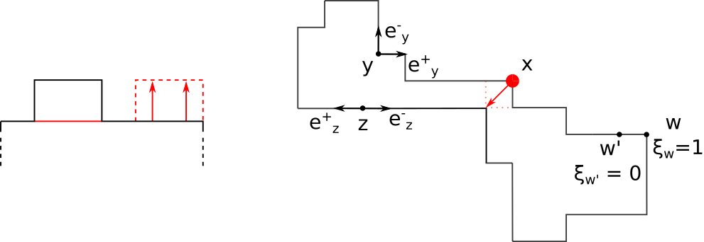
Figure 4: Left figure: two microscopic curves equal everywhere except at the north pole: the configuration represented by the black line has a pole containing $2$ blocks, the one with the red line a pole containing $6$ blocks. Initially, the droplet delimited by the black line contains the red droplet. A possible update after which the inclusion does not hold is represented in dashed red lines: the contour dynamics is not monotonous.
Right-figure: only looking at a neighbourhood of $x$, the update indicated by an arrow should be allowed, as the corresponding block has two neighbours in,and two neighbours out of the droplet. However, this update would make the curve non-simple, thus the resulting curve would not belong to $\Omega^{N}_{\text{mic}}$: the contour dynamics is therefore non local. The vectors ${\bf e}^{\pm}_{y},{\bf e}^{\pm}_{z}$ are indicated for two points $y,z$ of the interface. The edges $[y+{\bf e}^{-}_{y},y]$ and $[y,y+{\bf e}^{+}_{y}]$ are perpendicular: a block can be added or removed at $y$ (here, added). The same situation occurs at site $w$: the edge $[w,w+{\bf e}^{+}_{w}]$ is vertical, corresponding to $\xi_{v}=1$, while the edge $[w^{\prime},w]=[w+{\bf e}^{-}_{w},w]$ is horizontal, i.e. $\xi_{w^{\prime}}=0$.

Link with simple exclusion. The jump rates $c\big{(}\gamma^{N},(\gamma^{N})^{i}\big{)}$, $\gamma^{N}\in\Omega^{N}_{\text{mic}}$, $i\in(N^{-1}\mathbb{Z}^{*})^{2}$ involve the entire space $(N^{-1}\mathbb{Z}^{*})^{2}$, even though they vanish when $i$ is not at distance $1/(2N)$ from $\gamma^{N}$. It is possible to express these jump rates only in terms of points of the interface, which connects the contour dynamics to the symmetric simple exclusion process (henceforth SSEP) as we now explain. For $\gamma^{N}\in\Omega^{N}_{\text{mic}}$, let $V(\gamma^{N})$ denote the set of vertices of $\gamma^{N}$:

$$V(\gamma^{N}):=(N^{-1}\mathbb{Z})^{2}\cap\gamma^{N}.$$ (2.17)

If $x\in V(\gamma^{N})$, let ${\bf e}^{+}_{x}={\bf e}^{+}_{x}(\gamma)$ be the vector such that the edge with left extremity $x$ is given by $[x,x+{\bf e}^{+}_{x}]$, and ${\bf e}^{-}_{x}={\bf e}^{-}_{x}(\gamma)$ be the vector such that $[x+{\bf e}^{-}_{x},x]$ is the edge ending at $x$ (see Figure 4, and recall that interfaces are oriented clockwise). By definition of $\Omega^{N}_{\text{mic}}$, note that:

$$\|{\bf e}^{\pm}_{x}\|_{1}=\frac{1}{N}=\|{\bf e}^{\pm}_{x}\|_{2}.$$ (2.18)

Let $\xi_{x}=\xi_{x}(\gamma^{N})$ be the state of the edge $[x,x+{\bf e}^{+}_{x}]$, defined by:

$$\xi_{x}=1\quad\text{if }[x,x+{\bf e}^{+}_{x}]\text{ is vertical},\qquad\xi_{x}=0\quad\text{if }[x,x+{\bf e}^{+}_{x}]\text{ is horizontal}.$$ (2.19)

A block can be added/deleted to a droplet provided it has at least two neighbours of opposite colours, see Figure 3. This means that the interface has a corner at this block, i.e. there is a point $x\in V(\gamma^{N})$ (corresponding to the corner of the block) such that the two edges $[x+{\bf e}^{-}_{x},x]$ and $[x,x+{\bf e}^{+}_{x}]$ are perpendicular. Orthogonality of the two edges can be stated as follows:

$$\xi_{x+{\bf e}^{-}_{x}}(1-\xi_{x})+\xi_{x}(1-\xi_{x+{\bf e}^{-}_{x}})=1.$$ (2.20)

This condition coincides with the exclusion rule in a SSEP, provided each edge of $\gamma^{N}$ is associated with a site, and $\xi_{\cdot}$ is identified with the particle number (see the corresponding mapping in Figure 7 below). If $i\in(N^{-1}\mathbb{Z})^{2}$ is the centre of the block with corner $x$, define then $(\gamma^{N})^{x}$ as the curve $(\gamma^{N})^{i}$ of (2.13), and set:

$$c\big{(}\gamma^{N},(\gamma^{N})^{x}\big{)}={\bf 1}_{(\gamma^{N})^{x}\in\Omega^{N}_{\text{mic}}}c_{x}(\gamma^{N}),\qquad c_{x}(\gamma^{N}):=\frac{1}{2}\big{[}\xi_{x+{\bf e}^{-}_{x}}(1-\xi_{x})+\xi_{x}(1-\xi_{x+{\bf e}^{-}_{x}})\big{]}.$$ (2.21)

The indicator function above is related to the non-locality of the dynamics, see the right figure of Figure 4 and the second point of Remark 2.4. We will also say that "$x$ is flipped" to mean that the block with centre $i$ is added or deleted. The connection with the SSEP is further discussed in Section 2.4.
Recalling the jump rates at the poles in Definition 2.3, the generator $\mathcal{L}_{\beta}$ of the contour dynamics at $\beta>0$ then acts on functions $f:\Omega^{N}_{\text{mic}}\rightarrow\mathbb{R}$ according to:

$$\forall\gamma^{N}\in\Omega^{N}_{\text{mic}},\qquad N^{2}\mathcal{L}_{\beta}f(\gamma^{N})=N^{2}\sum_{x\in V(\gamma^{N})}{\bf 1}_{(\gamma^{N})^{x}\in\Omega^{N}_{\text{mic}}}c_{x}(\gamma^{N})\big{[}f\big{(}(\gamma^{N})^{x}\big{)}-f(\gamma^{N})]$$ (2.22)

$$+N^{2}\sum_{k=1}^{4}\sum_{\begin{subarray}{c}x\in V(\gamma^{N})\cap P_{k}(\gamma^{N})\\ x+{\bf e}^{\pm}_{x}\in P_{k}(\gamma^{N})\end{subarray}}\Big{[}{\bf 1}_{p_{k}(\gamma^{N})=2}{\bf 1}_{(\gamma^{N})^{-,k}\in\Omega^{N}_{\text{mic}}}\big{[}f\big{(}(\gamma^{N})^{-,k})-f(\gamma^{N})\big{]}+e^{-2\beta}\big{[}f\big{(}(\gamma^{N})^{+,x}\big{)}-f(\gamma^{N})\big{]}\Big{]}.$$

In (2.22), the first line corresponds to the SSEP-like updates, and the second line to the poles, with the last term corresponding to regrowth moves. Note the $N^{2}$ factor in the generator corresponding to a diffusive rescaling of time, which already appeared in the hydrodynamics (2.7).

2.2.3 Initial condition of the dynamics, topology and effective state space

Here, we define the initial condition of the dynamics. As we explain below, it is chosen in such a way that the contour dynamics is local for short times.

Definition 2.5 (Initial condition).

Let $\gamma^{\text{ref}}\subset\mathbb{R}^{2}$ be a Lipschitz Jordan curve satisfying Property 2.1. Let $\Gamma^{\text{ref}}$ be the associated droplet. Assume that $0$ is in the interior of $\Gamma^{\text{ref}}$:

$$\exists q>0,\quad\big{\{}x\in\mathbb{R}^{2}:\|x\|_{\infty}\leq q\big{\}}\subset\Gamma^{\text{ref}}.$$ (2.23)

Assume also that the poles of $\gamma^{\text{ref}}$ are sufficiently far away from one another:

$$\exists r>0,\forall 1\leq k\neq\ell\leq 4,\qquad d_{\infty}\big{(}P_{k}(\gamma^{\text{ref}}),P_{\ell}(\gamma^{\text{ref}})\big{)}\geq r,$$ (2.24)

where $d_{\infty}$ is the distance for the norm $\|\cdot\|_{\infty}$ on $\mathbb{R}^{2}$ (see (2.6)). Let $\Gamma^{\text{ref},N}$ be the droplet obtained by discretising $\Gamma^{\text{ref}}$ as follows:

$$\Gamma^{\text{ref},N}=\bigcup_{i\in(N^{-1}\mathbb{Z}^{*})^{2}:C_{i}\subset\Gamma^{\text{ref}}}C_{i},\qquad C_{i}:=i+\frac{1}{2N}[-1,1]^{2}.$$ (2.25)

Then $\gamma^{\text{ref},N}:=\partial\Gamma^{\text{ref},N}$ is a simple curve. For large enough $N\in\mathbb{N}^{*}$, up to adding a finite number of blocks at the poles to ensure each pole of $\gamma^{\text{ref},N}$ contains at least two blocks, we may assume $\gamma^{\text{ref},N}\in\Omega^{N}_{\text{mic}}$. The contour dynamics is started from $\gamma^{\text{ref},N}$.

Let us comment on the objects appearing in Definition 2.5.

Since $\gamma^{\text{ref}}$ is simple, the initial interface $\gamma^{\text{ref},N}$ has length bounded independently of $N$, and delimits a droplet with surface also bounded independently of $N$. This determines the scale at which interfaces evolve according to the contour dynamics: lengths and surfaces stay of order $1$ in $N$ for a diffusive amount of time, see Proposition 2.9.
The condition (2.24) is technical. It guarantees that, at the microscopic level, one can consider the dynamics around each pole independently of the other poles.
However, the assumption that $\gamma^{\text{ref}}$ is a simple curve has the following essential consequence: for large enough $N$, the situation of Figure 4 cannot occur as long as microscopic curves stay in a sufficiently small neighbourhood of the initial condition $\gamma^{\text{ref},N}$. This means that the contour dynamics is local for curves in that neighbourhood of the initial condition.
Indeed, $\gamma^{\text{ref}}$ being simple implies that there is $r^{\prime}>0$ such that, for any large enough $N\in\mathbb{N}^{*}$, if $\gamma^{N}\in\Omega^{N}_{\text{mic}}$ has associated droplet $\Gamma^{N}$, then:

$$d_{L^{1}}(\Gamma^{\text{ref}},\Gamma^{N})\leq(r^{\prime})^{2}\quad\Rightarrow\quad\gamma^{N},(\gamma^{N})^{x}\text{ are simple curves for each }x\in V(\gamma^{N}),$$ (2.26)

where the volume distance $d_{L^{1}}$ between bounded sets $A,B\subset\mathbb{R}^{2}$ is defined by:

$$d_{L^{1}}(A,B)=\int_{\mathbb{R}^{2}}\big{|}{\bf 1}_{A}-{\bf 1}_{B}\big{|}dudv.$$ (2.27)

The right-hand side of (2.26) ensures that the jump rates $c(\gamma^{N},(\gamma^{N})^{x})$ are given by the local function $c_{x}(\gamma^{N})$ defined in (2.21). The fact that the right-hand side of (2.26) can be obtained with a control of the volume distance $d_{L^{1}}$, rather than a stronger one such as the Hausdorff distance $d_{\mathcal{H}}$ (defined in (2.9)), is a consequence of the structure of curves in $\Omega$, see Definition 2.2.
Note also that properties (2.23)-(2.24)-(2.26) are satisfied for curves in a small neighbourhood of $\gamma^{\text{ref}}$: for each small enough $\zeta>0$, $\gamma\in B_{L^{1}}(\gamma^{\text{ref}},\zeta)$ implies that $\gamma$ satisfies (2.23)-(2.24)-(2.26) for some other $q,r,r^{\prime}>0$.

Notation: in the rest of the article, to avoid constantly alternating between interfaces and their associated droplets, we chose as much as possible to state results in terms of interfaces $\gamma,\tilde{\gamma}\in\Omega$ exclusively. In particular, we will use the convention:

$$d_{L^{1}}(\gamma,\tilde{\gamma}):=d_{L^{1}}(\Gamma,\tilde{\Gamma}).$$ (2.28)

As we now state, we shall work on a subset of the state space $\Omega$ on which interfaces satisfy the same three properties (2.23)-(2.24)-(2.26) as $\gamma^{\text{ref}}$ (with possibly different constants $q,r,r^{\prime}$), so that the contour dynamics is in particular local. Let us first collect these properties into one.

Property 2.6.

A curve $\gamma\in\Omega$ satisfies Property 2.6 if there are $\hat{q},\hat{r},\hat{r}^{\prime}>0$ for which $\gamma$ satisfies (2.23)-(2.24)-(2.26).

We could then carry out the study of the contour dynamics focussing on elements of $\Omega$ satisfying Property 2.6. Results in that direction are stated in Theorem 2.17.
However, this choice comes with difficulties at the level of the topology on trajectories. To simplify the exposition and focus on the probabilistic aspects of the droplet evolution, we therefore choose to restrict to just a small volume neighbourhood of $\gamma^{\text{ref}}$. In this sense, all results stated in Section 2.3 must be understood as short-time results, as we only consider interfaces close to the initial condition of the dynamics. The fact that interfaces do typically stay close to the initial condition for sufficiently short time is proven in Proposition 2.9.

Definition 2.7 (Effective state space).

The effective state space $\mathcal{E}$ is the subset of $\Omega$ made of curves $\gamma$ satisfying $d_{L^{1}}(\gamma^{\text{ref}},\gamma)\leq r_{0}^{2}$, with $r_{0}=\min\{q,r,r^{\prime}\}/2$, and $q,r,r^{\prime}$ respectively given by (2.23)-(2.24)-(2.26). At the microscopic level, we will consider elements of $\Omega^{N}_{\text{mic}}\cap\mathcal{E}$, meaning curves in a neighbourhood of the initial condition $\gamma^{\text{ref}}$. The jump rates of the contour dynamics for each such curve are local by the previous discussion.

Remark 2.8.

The factor $1/2$ in the definition of $r_{0}$ is chosen to ensure that elements of $\mathcal{E}$ must satisfy (2.23)-(2.24)-(2.26), for possibly different parameters $q,r,r^{\prime}$.  $\blacksquare$

Notation: to avoid confusion between microscopic and macroscopic interfaces in the following, whenever both microscopic and macroscopic interfaces are considered, microscopic interfaces are denoted with a superscript $N$: $\gamma^{N}\in\Omega^{N}_{\text{mic}}$, with associated droplet $\Gamma^{N}$. In that case, the letters $\gamma,\Gamma$ without the $N$ superscript are used for macroscopic objects.

2.2.4 Test functions and tilted dynamics

In the breakthrough paper [KOV89], a very powerful method was introduced to study large deviations for interacting particle systems. It relies on the introduction of suitable tilted dynamics. In our case, these dynamics are defined as follows. Consider the following set $\mathcal{C}$ of test functions:

$$\mathcal{C}=\big{\{}G\in C_{c}\big{(}\mathbb{R}_{+}\times\mathbb{R}^{2}\big{)}:\partial_{t}G,\partial_{i}G,\partial_{i}\partial_{j}G\in C_{c}(\mathbb{R}_{+}\times\mathbb{R}^{2}),(i,j)\in\{1,2\}^{2}\big{\}}.$$ (2.29)

In (2.29), the subscript $c$ means compactly supported. We will frequently write $G_{t}$ for the function $x\in\mathbb{R}^{2}\mapsto G(t,x)$, for $t\geq 0$. For $H\in\mathcal{C}$, define another (time-inhomogeneous) Markov chain with generator $N^{2}\mathcal{L}_{\beta,H}$ by modifying the jump rates as follows. If $\gamma\in\Omega$, recall that $\Gamma$ stands for the droplet associated with $\gamma$, and let:

$$\big{<}\Gamma,H_{t}\big{>}:=\int_{\Gamma}H_{t}(u,v)dudv,\qquad t\geq 0.$$ (2.30)

Then, for each $\gamma^{N},\tilde{\gamma}^{N}\in\Omega^{N}_{\text{mic}}\cap\mathcal{E}$ and associated droplets $\Gamma^{N},\tilde{\Gamma}^{N}$, the tilted jump rates are:

$$\forall t\geq 0,\qquad c^{H_{t}}(\gamma^{N},\tilde{\gamma}^{N}):=c(\gamma^{N},\tilde{\gamma}^{N})\exp\Big{[}N\big{<}\tilde{\Gamma}^{N},H_{t}\big{>}-N\big{<}\Gamma^{N},H_{t}\big{>}\Big{]}.$$ (2.31)

The probability measure associated with the speeded-up generator $N^{2}\mathcal{L}_{\beta,H}$ will be denoted by $\mathbb{P}^{N}_{\beta,H}$, or simply $\mathbb{P}^{N}_{\beta}$ when $H\equiv 0$ (recall that the diffusive, $N^{2}$ scaling is the correct one for motion by curvature). The corresponding expectations are denoted by $\mathbb{E}^{N}_{\beta,H},\mathbb{E}^{N}_{\beta}$ respectively.

2.3 Results

Our first result is a stability estimate. It states that, in the large $N$ limit, trajectories starting from the discretisation $\gamma^{\text{ref},N}$ of the curve $\gamma^{\text{ref}}$ of Definition 2.5 typically have length bounded independently of $N$, and stay close to $\gamma^{\text{ref}}$ in volume for short time.

Proposition 2.9.

Let $\beta>1$ and $H\in\mathcal{C}$. Then:

1. The length of an interface is of order $1$ in the following sense: for each time $T>0$, there are constants $C(\beta,H,T),C(H)>0$ such that:

   $$\forall A>0,\qquad\limsup_{N\rightarrow\infty}\frac{1}{N}\log\mathbb{P}^{N}_{\beta,H}\Big{(}\sup_{t\leq T}|\gamma^{N}_{t}|\geq A\Big{)}\leq-C(\beta,H,T)A+|\gamma^{\text{ref}}|\beta+C(H).$$ (2.32)

2. There is a time $t_{0}(\beta,H,\gamma^{\text{ref}})>0$ such that:

   $$\lim_{N\rightarrow\infty}\mathbb{P}^{N}_{\beta,H}\Big{(}\forall t\leq t_{0}(\beta,H,\gamma^{\text{ref}}),\gamma^{N}_{t}\in\mathcal{E}\Big{)}=1..$$ (2.33)

Proposition 2.9 tells us that, under the contour dynamics, typical interfaces evolve on (at least) a diffusive time scale. It thus makes sense to look for short time at microscopic trajectories in $\mathcal{E}$, i.e. in a neighbourhood of the initial condition $\gamma^{\text{ref},N}$. In all following results, we work with trajectories taking values in $\mathcal{E}$ at each time. The only exception is Theorem 2.17, where general trajectories are treated.

The second result, Proposition 2.10, concerns the role of the parameter $\beta$ in the contour dynamics. This result is perhaps the most striking feature of the contour dynamics. To state it, we need some notations. For $\gamma^{N}\in\Omega^{N}_{\text{mic}}\cap\mathcal{E},\ell\in\mathbb{N}^{*}$ and a vertex $x\in V(\gamma^{N})$, recall the definition (2.19) of the $\xi_{x}$, and denote by $\xi_{x}^{+,\ell}$ the quantity (see Figure 5):

$$\xi_{x}^{+,\ell}=\frac{1}{\ell+1}\sum_{\begin{subarray}{c}y\in V(\gamma^{N})\cap B_{1}(x,\ell/N)\\ y\geq x\end{subarray}}\xi_{y},$$ (2.34)

where $B_{1}(x,a)$ is the ball of centre $x$ and radius $a>0$ in 1-norm (2.6). Recall that $\gamma^{N}$ is an interface, i.e. a closed lattice path on $(N^{-1}\mathbb{Z})^{2}$, while $V(\gamma^{N})$ is the set of lattice points contained in $\gamma^{N}$. By $y\geq x$ we mean that $y$ is encountered after $x$ when travelling on $\gamma^{N}$ clockwise. The parameter $\ell$ will always be chosen much smaller than the number of edges in $\gamma$. We shall informally refer to $\xi_{x}^{+,\ell}$ as the slope (on the right-side of $x$). Define similarly the slope $\xi_{x}^{-,\ell}$ on the left of $x$ by averaging over points that are before $x$ on $\gamma^{N}$.

Proposition 2.10.

Choose $\beta>1$ and a time $T>0$. Then, for any bias $H\in\mathcal{C}$, any test function $G\in\mathcal{C}$ and any $\delta>0$, if $k\in\{1,3\}$:

$$\limsup_{\varepsilon\rightarrow 0}\limsup_{N\rightarrow\infty}\frac{1}{N}\log\mathbb{P}^{N}_{\beta,H}\bigg{(}\forall t\in[0,T],\gamma^{N}_{t}\in\mathcal{E};$$

$$\hskip 142.26378pt\bigg{|}\int_{0}^{T}G(t,L_{k}(\gamma^{N}_{t}))\big{(}\xi_{L_{k}(\gamma^{N}_{t})}^{\pm,\varepsilon N}-e^{-\beta}\big{)}dt\bigg{|}\geq\delta\bigg{)}=-\infty.$$ (2.35)

If on the other hand $k\in\{2,4\}$:

$$\limsup_{\varepsilon\rightarrow 0}\limsup_{N\rightarrow\infty}\frac{1}{N}\log\mathbb{P}^{N}_{\beta,H}\bigg{(}\forall t\in[0,T],\gamma^{N}_{t}\in\mathcal{E};$$

$$\hskip 142.26378pt\bigg{|}\int_{0}^{T}G(t,L_{k}(\gamma^{N}_{t}))\big{(}1-\xi_{L_{k}(\gamma^{N}_{t})}^{\pm,\varepsilon N}-e^{-\beta}\big{)}dt\bigg{|}\geq\delta\bigg{)}=-\infty.$$ (2.36)

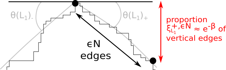
Figure 5: North pole of a curve with the proportion $\xi^{+,\varepsilon N}_{L_{1}}$ of vertical edges to the right of the pole. For drawing convenience, $\xi^{+,\varepsilon N}_{L_{1}}$ is assumed to be close to $e^{-\beta}$, which is true for its time average by Proposition 2.10. The corresponding angles $\theta(L_{1})_{\pm}$ are also drawn.

Proposition 2.10 shows that, as long as trajectories remain in the effective state space $\mathcal{E}$, the time average of the slopes on either side of the poles are fixed in terms of $\beta$. As we explain in Section 2.4, Proposition 2.10 can be understood as a statement that the pole dynamics has the same effect as reservoirs at density $e^{-\beta}$ or $1-e^{-\beta}$ in the simple exclusion process.

In the following, it will be useful to rephrase the condition on the slope described in Proposition 2.10 in terms of a condition involving macroscopic quantities. The corresponding formulation in terms of angles is the following. We shall say that a curve $\gamma\in\mathcal{E}$ has slope $e^{-\beta}$ at pole $k$ with $1\leq k\leq 4$ (see Figure 5) if the angle $\theta(L_{k}(\gamma)_{\pm})$ between the tangent vector ${\bf T}$ approaching $L_{k}(\gamma)$ from the left ($-$) or the right ($+$), and the vector ${\bf b}_{1}$, satisfies:

$$\tan\Big{(}\theta(L_{k}(\gamma)_{-})+\frac{(k-1)\pi}{2}\Big{)}=\frac{e^{-\beta}}{1-e^{-\beta}}=-\tan\Big{(}\theta(L_{k}(\gamma)_{+})+\frac{(k-1)\pi}{2}\Big{)}.$$ (2.37)

Hydrodynamic limit
Next, we investigate the typical evolution of interfaces following the contour dynamics with a bias $H\in\mathcal{C}$. We prove that they evolve according to an anisotropic motion by curvature as in (2.3), but with an influence of the parameter $\beta$. To prove such a result, a suitable topology on trajectories is required. In the proof of the hydrodynamic limit for the zero temperature stochastic Ising model in [LST14a]-[LST14], the authors prove uniform convergence in time for the topology associated with the Hausdorff distance (2.9). The Hausdorff distance between sets appears as a natural distance to put on the state space. Indeed, away from each pole, portions of the interface can be mapped to a SSEP (see Section 2.4). Hausdorff convergence of the interface can then be shown to be equivalent to weak convergence of the empirical measure in the associated SSEP, a topology in which hydrodynamics are known for this model.

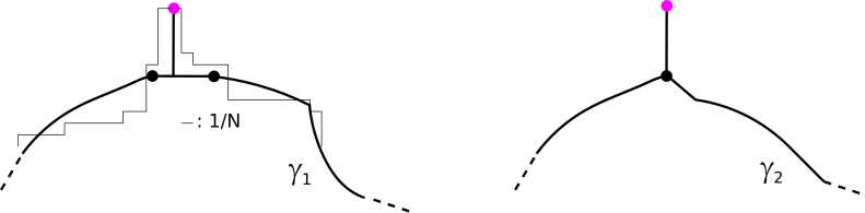
Figure 6: Portions of two simple curves $\gamma_{1},\gamma_{2}\in\Omega$, and of one element of a sequence of microscopic curves in $\Omega_{\text{mic}}^{N},N\in\mathbb{N}^{*}$ that converges to $\gamma_{1}$ in Hausdorff distance. The north poles of $\gamma_{1},\gamma_{2}$ are point-like, and represented by the magenta dots. The black dots delimit the flat portion on which the vertical line beneath the north poles of $\gamma_{1},\gamma_{2}$ rest. This portion may ($\gamma_{2}$) or may not ($\gamma_{1}$) be reduced to a point.

In the case of the contour model, the Skorokhod topology associated with the Hausdorff distance seems like a suitable choice. However, contrary to microscopic interfaces, which are simple curves with poles of length at least $2/N$, elements of $\Omega$ are however not necessarily simple curves (see Figure 6). Due to Property 2.1, a curve $\gamma\in\Omega$ is non simple when (and only when) one or more of its poles is at the extremity of a vertical or horizontal line. This means that one has to carefully control the contour dynamics at the poles. This is the main difficulty of the study, and in particular the Skorokhod topology associated with the Hausdorff distance turns out to be too strong. Instead, we separately control the trajectory of a droplet in volume distance $d_{L^{1}}$ (defined in (2.27)), and the time integral of the trajectory of its poles. For each $T>0$, define thus the set:

$$E([0,T],\Omega) :=D_{L^{1}}([0,T],\Omega)\cap\Big{\{}(\gamma_{t})_{t\leq T}:\int_{0}^{T}|\gamma_{t}|dt<\infty\Big{\}},$$

$$E([0,T],\mathcal{E}) :=E([0,T],\Omega)\cap\Big{\{}(\gamma_{t})_{t\leq T}:\gamma_{t}\in\mathcal{E}\text{ for }t\in[0,T]\Big{\}}.$$ (2.38)

Notation: we often use the subscript $\cdot$ (as in $\gamma_{\cdot}$ in (2.39)) to denote a trajectory, provided the time interval on which it is defined is clear from the context.
In Appendix B.2, we study the set $E([0,T],\mathcal{E})$ when equipped with the distance:

$$\forall\gamma_{\cdot},\tilde{\gamma}_{\cdot}\in E([0,T],\mathcal{E}),\qquad d_{E}(\gamma_{\cdot},\tilde{\gamma}_{\cdot}):=d^{S}_{L^{1}}(\gamma_{\cdot},\tilde{\gamma}_{\cdot})+\int_{0}^{T}d_{\mathcal{H}}(\gamma_{t},\tilde{\gamma}_{t})dt,$$ (2.39)

with $d_{L^{1}}^{S}$ the Skorokhod distance associated with $d_{L^{1}}$, and $d_{\mathcal{H}}$ the Hausdorff distance (2.9) on $\Omega$. Recall the convention (2.28) that the $L^{1}$ distance between two curves is by definition the $L^{1}$ distance between the droplets they delimit. Note that, since trajectories in $E([0,T],\mathcal{E})$ have almost always finite length, the associated droplets are almost always bounded subsets of $\mathbb{R}^{2}$, thus the time integral of the Hausdorff distance in (2.39) is well-defined.

Informally stated, the hydrodynamic limit result is then the following: the sequence $(\mathbb{P}^{N}_{\beta,H})_{N\in\mathbb{N}^{*}}$ of laws of the interface converges weakly to a probability measure concentrated on trajectories in $E([0,T],\mathcal{E})$ that are weak solutions, in the sense defined below in (2.41), of:

$$\begin{cases}\partial_{t}\gamma\cdot{\bf N}=a\partial^{2}_{s}\gamma\cdot{\bf N}-\mu H=ak-\mu H\quad&\text{away from the poles},\\ \gamma_{t}\text{ satisfies }\eqref{eq_tangente_angle_at_the_pole}\text{ at almost every }t\in[0,T],\end{cases}$$ (2.40)

with ${\bf N}$ the inwards normal vector, $a$ the anisotropy (2.4), $k$ the curvature, $\mu$ the mobility (2.43), and $s$ the arclength coordinate. The hydrodynamic limit result is formulated for sufficiently short time, see however Remark 2.12.

Proposition 2.11.

Let $\beta>1$, $H\in\mathcal{C}$ and $t_{0}=t_{0}(\beta,H,\gamma^{\text{ref}})$ be the time of Proposition 2.9. Then $(\mathbb{P}^{N}_{\beta,H})_{N}$ converges, in the weak topology associated with $d_{E}$, to a measure concentrated on trajectories in $E([0,t_{0}],\mathcal{E})$ that have almost always point-like poles, i.e. for a.e. $t\in[0,t_{0}]$, each $P_{k}(\gamma_{t}):=[L_{k}(\gamma_{t}),R_{k}(\gamma_{t})]$ is reduced to the point $L_{k}(\gamma_{t})=R_{k}(\gamma_{t})$, $1\leq k\leq 4$. Moreover, these trajectories are weak solutions of anisotropic motion by curvature with drift on $[0,t_{0}]$ in the following sense: for any $t\leq t_{0}$ and any test function $G$ in the set $\mathcal{C}$ defined in (2.29),

$$\big{<}\Gamma_{t},G_{t}\big{>}-\big{<}\Gamma^{\text{ref}},G_{0}\big{>}-\int_{0}^{t}\big{<}\Gamma_{t^{\prime}},\partial_{t^{\prime}}G_{t^{\prime}}\big{>}dt^{\prime} =\int_{0}^{t}\int_{\gamma_{t^{\prime}}\setminus\cup_{k}P_{k}(\gamma_{t^{\prime}})}\alpha(\theta(s))\partial_{s}G({t^{\prime}},\gamma_{t^{\prime}}(s))dsd{t^{\prime}}$$

$$\quad-\sum_{k=1}^{4}\int_{0}^{t}\Big{(}\frac{1}{2}-e^{-\beta}\Big{)}G({t^{\prime}},L_{k}(\gamma_{t^{\prime}}))d{t^{\prime}}$$

$$\quad+\int_{0}^{t}\int_{\gamma_{t^{\prime}}}\mu(\theta(s))(HG)({t^{\prime}},\gamma_{t^{\prime}}(s))dsd{t^{\prime}}.$$ (2.41)

Above, $\Gamma_{t}$ is the droplet associated with $\gamma_{t}$, $\big{<}\Gamma_{t},G_{t}\big{>}$ is the integral of $G_{t}$ on $\Gamma_{t}$ as in (2.30), and $s$ is the arclength coordinate on $\gamma_{t}$ at time $t\in[0,t_{0}]$. For each $\theta\in[0,2\pi]\setminus(\pi/2)\mathbb{Z}$, $\alpha$ is related to the anisotropy $a$ by $\alpha^{\prime}(\theta)=-a(\theta)$, where $a$ is defined in (2.4). One has:

$$\alpha(\theta)=\frac{a(\theta)}{2}\frac{\sin(2\theta)\cos(2\theta)}{|\sin(2\theta)|}=\frac{{\bf T}(\theta)\cdot{\bf b}_{1}{\bf T}(\theta)\cdot{\bf b}_{2}}{4\|{\bf T}(\theta)\|_{1}}\Big{[}\frac{1}{|{\bf T}(\theta)\cdot{\bf b}_{2}|}-\frac{1}{|{\bf T}(\theta)\cdot{\bf b}_{1}|}\Big{]},$$ (2.42)

with ${\bf T}(\theta)=\cos(\theta){\bf b}_{1}+\sin(\theta){\bf b}_{2}$. The quantity $\mu$ is the mobility of the model, defined by:

$$\mu(\theta):=\frac{|\sin(2\theta)|}{2(|\sin(\theta)|+|\cos(\theta)|)},\qquad\theta\in[0,2\pi].$$ (2.43)

Remark 2.12.

The time $t_{0}=t_{0}(\beta,H,|\gamma^{\text{ref}}|)$ until which Proposition 5.6 is proven does not make use of the structure of solutions to (2.41), and one can in fact improve the result as follows (this improvement is carried out in Section 5.2.3). Take $H\in\mathcal{C}$, $T\geq t_{0}(\beta,H,|\gamma^{\text{ref}}|)$, and make the following assumptions:

1. Equation (2.41) admits only one solution on $[0,T]$, call it $\gamma^{H}_{\cdot}=(\gamma^{H}_{t})_{t\leq T}$.

2. $\gamma^{H}_{\cdot}$ remains close to the initial condition $[0,T]$, in the sense:

   $$\exists\zeta_{H}>0,\qquad B_{d_{E}}\big{(}\gamma^{H}_{\cdot},\zeta_{H}\big{)}\subset E([0,T],\mathcal{E}).$$ (2.44)

Then $(\mathbb{P}^{N}_{\beta,H})_{N}$, as a sequence of measures on $E([0,T],\Omega)$, converges weakly to the measure $\delta_{\gamma^{H}_{\cdot}}$.  $\blacksquare$

Remark 2.13.

The term on the second line of (2.41) fixes the value of the slope at the pole of curves to the one prescribed by Proposition 2.10. Indeed, assume that the curvature $(k_{t})_{t\leq t_{0}}$ on a solution $(\gamma_{t})_{t\leq t_{0}}$ of (2.41) is, say, continuous and bounded on $\gamma_{t}\setminus\cup_{k}P_{k}(\gamma_{t})$ at each time $t\leq t_{0}$ (i.e. away from the poles). By definition, the tangent angle $s\mapsto\theta(s)=\theta(\gamma_{t}(s))$ then satisfies $\partial_{s}\theta(s)=-k_{t}(s)$ for each arclength coordinate $s$ corresponding to a point in $\gamma_{t}\setminus\cup_{k}P_{k}(\gamma_{t})$, with the $-$ sign due to the clockwise parametrisation of $\gamma_{t}$. Let $G\in\mathcal{C}$. Integrating $\alpha\partial_{s}G(t,\cdot)$ by parts on each region in (2.41) for a fixed $t\in[0,t_{0}]$, one then finds, by definition (2.42) of $\alpha$:

$$\int_{\gamma_{t}\setminus\cup_{k}P_{k}(\gamma_{t})}\alpha(\theta(s)) \partial_{s}G(t,\gamma_{t}(s))ds$$

$$\quad=\sum_{k=1}^{4}\big{[}\alpha\big{(}\theta(L_{k+1}(\gamma_{t}))_{-}\big{)}G(t,L_{k+1}(\gamma_{t}))-\alpha\big{(}\theta(R_{k}(\gamma_{t}))_{+}\big{)}G(t,R_{k}(\gamma_{t}))\big{]}$$

$$\qquad-\int_{\gamma_{t}\setminus\cup_{k}P_{k}(\gamma_{t})}a(\theta(s))k(\gamma_{t}(s))G(t,\gamma_{t}(s))ds.$$ (2.45)

Since $L_{k}(\gamma_{t})=R_{k}(\gamma_{t})$ for each $k$ and almost every $t\in[0,t_{0}]$, the sum in (2.45) compensates the second line of (2.41) provided $\alpha\big{(}\theta(L_{k+1}(\gamma_{t}))_{-}\big{)}=1/4-e^{-\beta}/2=-\alpha\big{(}\theta(L_{k}(\gamma_{t}))_{+}\big{)}$. It can be shown that this condition means that the tangent angle on either side of each pole must satisfy (2.37).  $\blacksquare$

Large deviations
We obtain upper-bound large deviations for the contour dynamics at each $\beta>1$. Assuming solutions of (2.41) to be unique, lower-bound large deviations can also be derived. Upper and lower bounds match for suitably regular trajectories. Specific to our model is, again, the control of the poles of the curves.
Let $T>0$ and $\beta>1$. Given a trajectory $\gamma_{\cdot}\in E([0,T],\mathcal{E})$ with associated droplets $(\Gamma_{t})_{t\leq T}$, define, recalling that $L_{k},R_{k}$ are the extremities of the pole $P_{k}$:

$$\ell^{\beta}_{H}(\gamma_{\cdot}) =\big{<}\Gamma_{T},H_{T}\big{>}-\big{<}\Gamma^{\text{ref}},H_{0}\big{>}-\int_{0}^{T}\big{<}\Gamma_{t},\partial_{t}H_{t}\big{>}dt-\int_{0}^{T}dt\int_{\gamma_{t}\setminus\cup_{k}P_{k}(\gamma_{t})}\alpha(\theta(s))\partial_{s}H(t,\gamma_{t}(s))ds$$

$$\hskip 99.58464pt+\Big{(}\frac{1}{4}-\frac{e^{-\beta}}{2}\Big{)}\int_{0}^{T}\sum_{k=1}^{4}\big{[}H(t,L_{k}(\gamma_{t}))+H(t,R_{k}(\gamma_{t}))\big{]}dt.$$ (2.46)

Define also:

$$J^{\beta}_{H}(\gamma_{\cdot})=\ell^{\beta}_{H}(\gamma_{\cdot})-\frac{1}{2}\int_{0}^{T}\int_{\gamma_{t}}\mu(\theta(s))H^{2}(t,\gamma_{t}(s))dsdt,\qquad\gamma_{\cdot}\in E([0,T],\mathcal{E}),$$ (2.47)

where the mobility $\mu$ is defined in (2.43).
To build the rate function, we will have to restrict the state space to control the behaviour of the poles. Introduce thus the subset $E_{pp}([0,T],\mathcal{E})\subset E([0,T],\mathcal{E})$ of trajectories with almost always point-like poles:

$$E_{pp}([0,T],\mathcal{E})=\bigg{\{}\gamma_{\cdot}\in E([0,T],\mathcal{E}):\sum_{k=1}^{4}\int_{0}^{T}\|L_{k}(\gamma_{t})-R_{k}(\gamma_{t})\|_{1}dt=0\bigg{\}}.$$ (2.48)

Recall that $R_{k}$ $(L_{k})$ is the right (left) extremity of pole $k\in\{1,...,4\}$. Let us now define the rate function $I_{\beta}(\gamma_{\cdot}|\gamma^{\text{ref}})$ for trajectories $\gamma_{\cdot}\in E([0,T],\mathcal{E})$:

$$I_{\beta}(\gamma_{\cdot}|\gamma^{\text{ref}})=\begin{cases}\sup_{H\in\mathcal{C}}J_{H}^{\beta}(\gamma_{\cdot})\quad&\text{if }\gamma_{\cdot}\in E_{pp}([0,T],\mathcal{E}),\\ +\infty&\text{otherwise.}\end{cases}$$ (2.49)

Remark 2.14.

• It is possible by Proposition 2.10 to enforce that only trajectories with slope $e^{-\beta}$ at the poles at almost every time have finite rate function. One would expect this condition to already be present in (2.49), but the very weak topology at the poles makes it more complicated to see than e.g. for a SSEP with reservoirs, as done in [BLM09].

• If $\beta=\infty$ and $\gamma_{\cdot}$ is a sufficiently regular trajectory in $C([0,T],\mathcal{E})$ starting from $\gamma^{\text{ref}}$ (say, with well-defined, continuous and bounded normal speed and curvature at each time $t\in(0,T]$), then setting $\beta=\infty$ in (2.49) one formally obtains:

  $$I_{\infty}(\gamma_{\cdot}|\gamma^{\text{ref}})=\frac{1}{2}\int_{0}^{T}\int_{\gamma_{t}}\frac{\Big{(}v\big{(}\gamma_{t}(s)\big{)}-a\big{(}\theta(s)\big{)}k\big{(}\gamma_{t}(s)\big{)}\Big{)}^{2}}{\mu\big{(}\theta(s)\big{)}}dsdt.$$ (2.50)

  As conjectured in (1.4), the rate function $I_{\infty}(\cdot|\gamma^{\text{ref}})$ thus measures the quadratic cost of deviations from anisotropic motion by curvature. At $\beta<\infty$, $I_{\beta}(\cdot|\gamma^{\text{ref}})$ can also be written in the form (2.50), but only for trajectories that are not smooth: they must have kinks at the poles, in the sense that they satisfy the condition (2.37) at almost every time.  $\blacksquare$

Define the set $\mathcal{A}_{\beta,T}\subset E([0,T],\mathcal{E})$ of trajectories with almost always point-like poles which can be obtained as a solution of the anisotropic motion by curvature with a smooth drift $H\in\mathcal{C}$ (2.41):

$$\mathcal{A}_{\beta,T}=\Big{\{}\gamma_{\cdot}\in E_{pp}([0,T],\mathcal{E}): \text{ there is a bias }H\in\mathcal{C}\text{ such that }\eqref{eq_formulation_faible_avec_der_en_temps}\text{ has a}$$

$$\text{ unique solution in }E([0,T],\mathcal{E})\text{, and this solution is }\gamma_{\cdot}\Big{\}}.$$ (2.51)

Theorem 2.15.

Let $T>0$ and $\beta>1$. For any closed set $C\subset E([0,T],\mathcal{E})$:

$$\limsup_{N\rightarrow\infty}\frac{1}{N}\log\mathbb{P}^{N}_{\beta}\big{(}\gamma^{N}_{\cdot}\in C\big{)}\leq-\inf_{C}I_{\beta}(\cdot|\gamma^{\text{ref}}).$$ (2.52)

Moreover, for any open set $O$ with $O\subset E([0,T],\mathcal{E})$:

$$\liminf_{N\rightarrow\infty}\frac{1}{N}\log\mathbb{P}^{N}_{\beta}\big{(}\gamma^{N}_{\cdot}\in O\big{)}\geq-\inf_{O\cap\mathcal{A}_{\beta,T}}I_{\beta}(\cdot|\gamma^{\text{ref}}).$$ (2.53)

Remark 2.16.

• The set $\mathcal{A}_{\beta,T}$ is expected to contain a large class of trajectories. In the $\beta=\infty$ case, it would for instance contain all classical solutions of the equation $v=ak-\mu H$, $H\in\mathcal{C}$, which can be studied by the method of [LST14a][LST14]. When $\beta<\infty$ however, even classical solutions of (2.40) are extremely difficult to study due to the poles. A fortiori, the study of uniqueness and regularity of solutions of the weak formulation (2.41) is difficult.

• A possible application of Theorem 2.15 is the analysis of metastability. For instance, applying a small, uniform field of the form $h/N$, $h>0$, one can use Theorem 2.15 to study the optimal trajectory for a nucleated droplet to cover the whole space.
  One can also ask about the typical speed at which such a droplet grows. This speed is conjectured to be proportional to the size of the applied field [SS98], i.e. of order $1/N$. For the contour dynamics, curves move diffusively, which readily confirms the conjecture. The interested reader will find much more on metastability and its relation to large deviations in the book [OV05].  $\blacksquare$

We conclude this section by rephrasing Theorem 2.15 in a more general context. Elements of $\mathcal{E}$ are, by assumption (see Definition 2.7), in a small neighbourhood of the initial condition $\gamma^{\text{ref}}$ for the volume distance. As claimed above Definition 2.7 of $\mathcal{E}$, however, it only matters for our arguments that curves have the same characteristics as $\gamma^{\text{ref}}$ (corresponding to curves satisfying Property 2.6), not that they be close to it (i.e. in $\mathcal{E}$). The reason why we focus on $\mathcal{E}$ is to avoid topological difficulties. Consequently, the next theorem improves Theorem 2.15 for trajectories possibly far from $\gamma^{\text{ref}}$, but satisfying the same Property 2.6 as $\gamma^{\text{ref}}$ at each time.

To state it, assume that $J^{\beta}_{H}$ is defined on the entire space $E([0,T],\Omega)$ (rather than $E([0,T],\mathcal{E})$) with the same expression (2.47). The rate function $I_{\beta}(\cdot|\gamma^{\text{ref}})$ is correspondingly given for $\gamma_{\cdot}\in E([0,T],\Omega)$ by:

$$I_{\beta}(\gamma_{\cdot}|\gamma^{\text{ref}})=\begin{cases}\sup_{H\in\mathcal{C}}J_{H}^{\beta}(\gamma_{\cdot})\quad&\text{if }\gamma_{\cdot}\text{ has almost always point-like poles,}\\ +\infty&\text{otherwise.}\end{cases}$$ (2.54)

Similarly, $\mathcal{A}_{\beta,T}$ is now assumed to contain trajectories in $E([0,T],\Omega)$ with almost always point-lie poles and that satisfy Property 2.6 at each time, rather than trajectories in $E_{pp}([0,T],\mathcal{E})$.

Theorem 2.17.

Let $\beta>1$, and let $\bar{\gamma}_{\cdot}\in E([0,T],\Omega)$ be such that $\bar{\gamma}_{t}$ satisfies Property 2.6 at each time $t\leq T$. Then:

$$\limsup_{\zeta\rightarrow 0}\limsup_{N\rightarrow\infty}\frac{1}{N}\log\mathbb{P}^{N}_{\beta}\big{(}\gamma^{N}_{\cdot}\in B_{d_{E}}\big{(}\bar{\gamma}_{\cdot},\zeta\big{)}\big{)}\leq-I_{\beta}(\bar{\gamma}_{\cdot}|\gamma^{\text{ref}}).$$ (2.55)

Moreover, if $\bar{\gamma}_{\cdot}$ is in $\mathcal{A}_{\beta,T}$, then:

$$\liminf_{\zeta\rightarrow 0}\liminf_{N\rightarrow\infty}\frac{1}{N}\log\mathbb{P}^{N}_{\beta}\big{(}\gamma^{N}_{\cdot}\in B_{d_{E}}\big{(}\bar{\gamma}_{\cdot},\zeta\big{)}\big{)}\geq-I_{\beta}(\bar{\gamma}_{\cdot}|\gamma^{\text{ref}}).$$ (2.56)

2.4 Heuristics on large deviations: link with the SSEP

In this section, we highlight the relationship between the contour dynamics away from the poles and the SSEP. This relationship is a central guideline of the proof of the large deviations (the structure of the proof is detailed in Section 2.5). A heuristic derivation of the rate function of Theorem 2.15 is also proposed using the link with the SSEP.

Take a curve $\gamma^{N}\in\Omega^{N}_{\text{mic}}$ (see Definition 2.2) as in Figure 2. By Property 2.1, $\gamma^{N}$ can be split into four regions. Let $1\leq k\leq 4$. Rotating the canonical reference frame $({\bf b}_{1},{\bf b}_{2})$ by $\pi/4+(k-1)\pi/2$, region $k$ of the boundary is turned into the graph of a $1$-Lipschitz function $f^{N,k}$, which has slope $\pm 1$. The $k=1$ case is illustrated on Figure 7.
To obtain a particle configuration with at most one particle per site, proceed then as follows. With each edge in the original region, associate a site. Put a particle in the site if the corresponding edge corresponds to a position in which $f^{N,k}$ has slope $-1$, and no particle if $f^{N,k}$ has slope $1$. Updates of the contour dynamics away from the poles then correspond to SSEP updates, as remarked in (2.20).

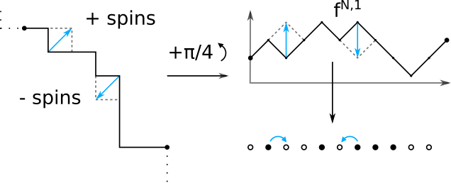
Figure 7: The mapping from a portion of region $1$ (left figure), delimited by the two big black dots, to the graph of a Lipschitz function $f^{N,1}$ (upper right figure). This Lipschitz function is then mapped to a particle configuration (lower right figure). Each edge of the initial interface corresponds to a possible site for particles. In the portion of the original interface delimited by the black dots, dynamical updates (blue arrows) do not change the length of the portion. These updates are precisely mapped to SSEP moves.

In this picture, if $\eta^{N,k}=(\eta^{N,k}(i))_{i}$ denotes the particle configuration obtained in region $k$ by the above mapping, with $i\in\mathbb{N}$ enumerating the particles sites in region $k$ with the convention that the first site has label $0$, then $\eta^{N,k}$ is associated with $f^{N,k}$ through:

$$\eta^{N,k}(i):=\frac{1}{2}+\frac{(-1)^{k}\sqrt{2}N}{2}\Big{[}f^{N,k}\Big{(}\frac{i+1/N}{\sqrt{2}}\Big{)}-f^{N,k}\Big{(}\frac{i}{\sqrt{2}}\Big{)}\Big{]}.$$ (2.57)

Above, the $(-1)^{k}$ comes from the fact that the $f^{k}$ are defined in different referent frames ($f^{1}$ in $({\bf b}_{-\pi/4},{\bf b}_{\pi/4})$, $f^{2}$ in $({\bf b}_{-3\pi/4},{\bf b}_{-\pi/4})$, etc.). The $\sqrt{2}$’s arise because the axes of all these reference frames are tilted by $\pi/4$ compared to the usual axes passing through ${\bf b}_{1},{\bf b}_{2}$.
At the macroscopic level, region $k$ ($1\leq k\leq 4$) of a curve $\gamma\in\mathcal{E}$ can similarly be seen as the graph of a function $f^{k}$ on an interval $I^{k}=[a^{k},b^{k}]$, with ($R_{k+1}:=R_{1}$ if $k=4$):

$$a^{k}:=L_{k}\cdot{\bf b}_{\pi/4-k\pi/2},\qquad b_{k}=R_{k+1}\cdot{\bf b}_{\pi/4-k\pi/2}$$ (2.58)

The function $f^{k}$ can then be associated with a "particle density" $\rho^{k}$ according to:

$$\rho^{k}(u):=\frac{1+(-1)^{k}\partial_{u}f^{k}(u/\sqrt{2})}{2},\qquad u\in I^{k}.$$ (2.59)

Through this correspondence, the contour dynamics inside each region of an interface can be viewed as a SSEP. The dynamics at the poles (deletion or growth of two blocks at respective rates 1 and $e^{-2\beta}$) can then be viewed as a boundary dynamics that couples these SSEP. Indeed, in Proposition 2.10, we saw that the dynamics at each pole acts like a moving reservoir, fixing the density of particles at the extremity of each SSEP in terms of $\beta$. As a first, informal approximation, it thus makes sense to consider the contour dynamics as four SSEP coupled with reservoirs.

For a SSEP connected with reservoirs, the large deviation rate function is known to give finite weight only to trajectories which have the correct value of the density at each time [Ber+03]. For the contour dynamics, one then expects the following: let $\gamma_{\cdot}\in E([0,T],\mathcal{E})$. Then the contour dynamics rate function should be infinite unless:

$$\forall t\in[0,T],\qquad\rho^{k}_{t}\big{(}a^{k}(\gamma_{t})\big{)}=e^{-\beta}=1-\rho^{k}_{t}\big{(}b^{k}(\gamma_{t})\big{)},\quad 1\leq k\leq 4.$$ (2.60)

Moreover, on region $k$, say $k=1$ for definiteness, the rate function obtained in [Ber+03] on a fixed domain size could formally be written as:

$$I_{SSEP,1}\big{(}(\rho^{1}_{t})_{t\leq T}|(\rho^{0})^{1}\big{)}=\int_{0}^{T}\int_{a^{1}(\gamma_{t})}^{b^{1}(\gamma_{t})}\frac{\big{(}\partial_{t}f^{1}-(1/4)\Delta f^{1}\big{)}^{2}}{2\rho^{1}(1-\rho^{1})}\sqrt{2}dudt.$$ (2.61)

Note that, using the continuity relation $\partial_{t}\rho+\partial_{u}j=0$ where $j$ is the macroscopic current of particles, the quantity $\partial_{t}f$ corresponds to one half of the current. Note again the $\sqrt{2}$ factor in (2.61) due to the fact that $f^{1}$ is defined in a tilted reference frame.

Proving that (2.61) indeed corresponds to the cost that the first region of curves have the trajectory $\rho^{1}_{\cdot}$ is very complicated, due to the varying size of each SSEP because of the motion of the poles. Let us however explain why (2.61) indeed corresponds to the contribution of region 1 to the rate function $I_{\beta}(\gamma_{\cdot}|\gamma^{\text{ref}})$ of Theorem 2.15, at least for sufficiently nice trajectories $\gamma_{\cdot}$ satisfying (2.60). We stress again that the following heuristics is not directly useful for the proof, but instead serves as a useful intuition.
To interpret (2.61), let us express its right-hand side as a line integral. The tangent vector at a point $x=u{\bf b}_{-\pi/4}+f^{1}(u){\bf b}_{\pi/4}$ of region $1$, corresponding to an angle $\theta=\theta(x)\in[0,2\pi]$, reads:

$${\bf T}(\theta)=\cos(\theta){\bf b}_{1}+\sin(\theta){\bf b}_{2}=\big{[}1+(\partial_{u}f^{1})^{2}\big{]}^{-1/2}\big{(}{\bf b}_{-\pi/4}+\partial_{u}f^{1}{\bf b}_{\pi/4}\big{)}.$$ (2.62)

With (2.62), one can check, as done in Section 3.3. of [LST14], that the heat equation for $f^{1}$ indeed corresponds to anisotropic motion by curvature (2.3). On the other hand, (2.59) and (2.62) yield for $\rho^{1}(1-\rho^{1})$:

$$\rho^{1}(1-\rho^{1})=\frac{1}{4}\big{(}1-(\partial_{u}f^{1})^{2}\big{)}=\frac{1}{\sqrt{2\big{[}1+(\partial_{u}f^{1})^{2}\big{]}}}\mu(\theta),$$ (2.63)

with $\mu$ the mobility coefficient obtained by Spohn [Spo93]:

$$\mu(\vartheta):=\frac{|\sin(2\vartheta)|}{2(|\sin(\vartheta)|+|\cos(\vartheta)|)}=\frac{|{\bf T}(\vartheta)\cdot{\bf b}_{1}||{\bf T}(\vartheta)\cdot{\bf b}_{2}|}{\|{\bf T}(\vartheta)\|_{1}},\qquad\vartheta\in[0,2\pi].$$ (2.64)

Using the relation $ds=[1+(\partial_{u}f^{1})^{2}]^{1/2}du$ between $x$ and the arclength coordinate $s$ and generalising the above discussion to the other three regions, (2.61) yields for the conjectured rate function $I^{\text{heur}}_{\beta}(\cdot|\gamma^{\text{ref}})$ of the contour dynamics:

$$I^{\text{heur}}_{\beta}\big{(}\gamma_{\cdot}|\gamma^{\text{ref}}\big{)}=\int_{0}^{T}\int_{\gamma_{t}}\frac{\big{(}v-ak)^{2}}{2\mu}dsdt.$$ (2.65)

This is indeed the rate function of Theorem 2.15 for trajectories satisfying the boundary conditions (2.60) (compare with the $\beta=\infty$ case in (2.50), where the formula is the same, but for smooth trajectories rather than those satisfying the boundary conditions (2.60)). The analogy (2.61) with the SSEP thus gives the correct rate function at a formal level.
To establish Theorem 2.15, we will have to look at the contour dynamics both at, and away from the poles simultaneously. This makes it difficult to directly use this analogy with the SSEP at microscopic level. However, it is constantly used as a guideline throughout the proofs.

2.5 Outline of the proof of large deviations

The proof of Theorem 2.15 is structured as follows.

• Before looking at rare events specifically, an understanding of the dynamics at the poles is required. This is perhaps the most difficult part of the paper, and is the object of the technical Section 6. In particular, we show there that poles behave like reservoirs in the sense of Proposition 2.10.

• The proof of large deviations starts in Section 3. Following the standard techniques of [KOV89] (see also Chapter 10 in [KL99]), we compute the Radon-Nikodym derivative between the original dynamics, and the dynamics tilted by a bias $H\in\mathcal{C}$ introduced in (2.31). To avoid pathological issues with the contour dynamics such as non-locality, the computation is carried out for trajectories with values in $\mathcal{E}$, with $\mathcal{E}$ the effective state space of Definition 2.7.
  The computation at the microscopic level is inspired by the link with the SSEP as highlighted in Figure 7. This link is useful to perform discrete integration by parts and replacement lemma-type estimates. The resulting expressions are not easily interpreted as line integrals involving tangent vectors. This interpretation is carried out in a second time, similarly to what was done at the macroscopic level to go from SSEP to curves in Section 2.4.

• Section 4 contains upper bound large deviations. The proof technique is standard, and consists in estimating the cost of tilting the dynamics by a bias $H\in\mathcal{C}$. The added difficulty comes from the need to control the poles. The poles in particular prevent the functional $J^{\beta}_{H}$, from which the rate function is built, from having nice continuity properties, even for trajectories taking values in the effective state space $\mathcal{E}$ of Definition 2.7. Continuity is recovered by proving that trajectories must have kinks at the poles in the sense of Proposition 2.10. Proving this fact, however, requires improved estimates compared to those giving Proposition 2.10. These improvements are carried out in Appendix B.3.

• Section 5 contains the lower bound, which amounts to hydrodynamic limits for the tilted processes, i.e. Proposition 2.11. As a first step, we need to make sure that the (tilted) contour dynamics takes a diffusive time to exit $\mathcal{E}$, i.e. we prove the short-time stability result of Proposition 2.9. The hydrodynamic limit results are then obtained in two steps: first in short time using the stability result of Proposition 2.9. Secondly, by extending the hydrodynamic limit to longer times through an iteration procedure.

3 Change of measures

3.1 Motivations

To investigate rare events, we are going to consider tilted probability measures, as in Chapter 10 of [KL99]. Fix a time $T>0$ throughout the rest of Section 3, and introduce a magnetic field $H\in\mathcal{C}$ ($\mathcal{C}$ is defined in (2.29)), so that for any measurable set $X$ of trajectories:

$$\mathbb{P}^{N}_{\beta}(\gamma^{N}_{\cdot}\in X)=\mathbb{E}^{N}_{\beta}[{\bf 1}_{\gamma^{N}_{\cdot}\in X}]=\mathbb{E}^{N}_{\beta,H}\big{[}(D^{N}_{\beta,H})^{-1}{\bf 1}_{\gamma^{N}_{\cdot}\in X}\big{]},$$ (3.1)

where $D^{N}_{\beta,H}=d\mathbb{P}^{N}_{\beta,H}/d\mathbb{P}^{N}_{\beta}$ is the Radon-Nikodym derivative until time $T$, acting on a trajectory $\gamma^{N}_{\cdot}=(\gamma^{N}_{t})_{t\leq T}\subset\Omega^{N}_{\text{mic}}$ delimiting droplets $(\Gamma^{N}_{t})_{t\leq T}$ according to (see Appendix A.7 in [KL99]):

$$N^{-1}\log D^{N}_{\beta,H}(\gamma^{N}_{\cdot}) =\big{<}\Gamma^{N}_{T},H_{T}\big{>}-\big{<}\Gamma^{N}_{0},H_{0}\big{>}$$

$$\quad-\int_{0}^{T}e^{-N\big{<}\Gamma^{N}_{t},H_{t}\big{>}}\big{(}\partial_{t}+N^{2}\mathcal{L}_{\beta}\big{)}e^{N\big{<}\Gamma^{N}_{t},H_{t}\big{>}}dt.$$ (3.2)

In (3.2), recall that, for a domain $\Gamma^{N}$ with boundary $\gamma^{N}\in\Omega_{\text{mic}}^{N}$ and a bounded $J:\mathbb{R}^{2}\rightarrow\mathbb{R}$, we write $\big{<}\Gamma^{N},J\big{>}$ for $\int_{\Gamma^{N}}J(u,v)dudv$. The rest of Section 3 is devoted to the computation of $N^{2}e^{-N\big{<}\Gamma^{N}_{t},H_{t}\big{>}}\mathcal{L}_{\beta}e^{N\big{<}\Gamma^{N}_{t},H_{t}\big{>}}$ for $t\leq T$.

3.2 Action of the generator

Take an interface $\gamma^{N}\in\Omega^{N}_{\text{mic}}\cap\mathcal{E}$, and as usual let $\Gamma^{N}$ denote the associated droplet. In view of the form (2.49) of the rate function, the quantity $N^{2}e^{-N\big{<}\Gamma^{N},H_{t}\big{>}}\mathcal{L}_{\beta}e^{N\big{<}\Gamma^{N},H_{t}\big{>}}$ will lead to line integrals on $\gamma^{N}$, as well as boundary terms involving the poles. We will obtain such an expression in two steps. The first step relies on microscopic computations and replacement of local quantities by local averages, guided by the link of Section 2.4 with the SSEP. The second step is the interpretation of the resulting quantities in terms of line integrals. We first state a result involving discretised line integrals (Proposition 3.2). The continuous counterpart, Proposition 3.11, is presented and proven later.

To state Proposition 3.2, let us fix some notations. For $x\in V(\gamma^{N})$, $\varepsilon>0$ and $N\in\mathbb{N}^{*}$, the local density of vertical edges $\xi_{x}^{\varepsilon N}$ is defined as:

$$\xi_{x}^{\varepsilon N}=\frac{1}{2\varepsilon N+1}\sum_{y\in B_{1}(x,\varepsilon)\cap V(\gamma^{N})}\xi_{y}.$$ (3.3)

The ball $B_{1}(x,\varepsilon)$ is taken with respect to the $1$-norm $\|\cdot\|_{1}$ (recall (2.6)), and we assume that $\varepsilon N$ is an integer for simplicity. In our case, it will be convenient to write $\xi_{x}^{\varepsilon N}$ as a function of the tangent vector at $x$. Recall that we always enumerate elements of $V(\gamma^{N})$ clockwise and that ${\bf e}^{+}_{x}$ is the microscopic tangent vector with norm $1/N$ given in (2.18). The direction of ${\bf e}^{+}_{x}$ is fixed by the region $x$ belongs to. For instance, if $x$ belongs to the first region and $y$ to the second:

$$N{\bf e}^{+}_{x}=(1-\xi_{x}){\bf b}_{1}-\xi_{x}{\bf b}_{2},\qquad N{\bf e}^{+}_{y}=-(1-\xi_{y}){\bf b}_{1}-\xi_{y}{\bf b}_{2}.$$ (3.4)

A representation of the vector ${\bf e}^{+}_{x}$ is given later on, in Figure 8. The following definition will be used below to keep track of the different signs depending on the region.

Definition 3.1.

For $\gamma^{N}\in\Omega^{N}_{\text{mic}}$, recall that ${\bf b}_{\theta}$ for $\theta\in[0,2\pi]$ is the vector defined in (2.10). Define then a vector ${\bf m}(\gamma^{N}):\gamma^{N}\setminus\cup_{k}P_{k}(\gamma^{N})\rightarrow\mathbb{R}^{2}$ to be constant on each region, and given by:

$$\forall x\in\gamma^{N}\setminus\cup_{k}P_{k}(\gamma^{N}),\qquad{\bf m}(x):={\bf m}(\gamma^{N},x)=\begin{cases}(-1,-1)\quad&\text{if }x\text{ is in region }1,\\ (-1,1)\quad&\text{if }x\text{ is in region }2,\\ (1,1)\quad&\text{if }x\text{ is in region }3,\\ (1,-1)\quad&\text{if }x\text{ is in region }4.\end{cases}$$ (3.5)

If $x$ is at 1-distance at least $\varepsilon$ to the poles, then all vertices in $B_{1}(x,\varepsilon)$ are in the same region. Define then the averaged tangent vector ${\bf t}^{\varepsilon N}_{x}$ on the ball $B_{1}(x,\varepsilon)$:

$${\bf t}^{\varepsilon N}_{x}=\frac{N}{2\varepsilon N+1}\sum_{y\in B_{1}(x,\varepsilon)\cap V(\gamma^{N})}{\bf e}^{+}_{y}\in\Big{\{}\zeta_{1}(1-\xi^{\varepsilon N}_{x}){\bf b}_{1}+\zeta_{2}\xi^{\varepsilon N}_{x}{\bf b}_{2}:\zeta_{1},\zeta_{2}\in\{-,+\}\Big{\}}.$$ (3.6)

The signs in (3.6) still only depend on the region of $\gamma^{N}$ that $x$ belongs to. For instance, if $B_{1}(x,\varepsilon)\cap\gamma^{N}$ is included in the first region,

$$N{\bf e}^{+}_{x}=(1-\xi_{x}){\bf b}_{1}-\xi_{x}{\bf b}_{2}\ \Rightarrow\ {\bf t}^{\varepsilon N}_{x}=(1-\xi^{\varepsilon N}_{x}){\bf b}_{1}-\xi^{\varepsilon N}_{x}{\bf b}_{2}.$$ (3.7)

We stress the fact that ${\bf t}^{\varepsilon N}_{x}$ is a unit vector in $1$-norm, but not in $2$-norm: $\|{\bf t}^{\varepsilon N}_{x}\|_{1}=1\neq\|{\bf t}^{\varepsilon N}_{x}\|_{2}$. This has important consequences later on, see Section 3.2.3. It will be useful to introduce the $2$-norm and $2$-normalised tangent vector:

$$\forall x\in V(\gamma^{N}),\qquad\mathsf{v}^{\varepsilon N}_{x}:=\|{\bf t}^{\varepsilon N}_{x}\|_{2},\qquad{\bf T}^{\varepsilon N}_{x}={\bf t}^{\varepsilon N}_{x}/\mathsf{v}^{\varepsilon N}_{x}.$$ (3.8)

As $\|{\bf t}^{\varepsilon N}\|_{1}=1$, we get:

$$\mathsf{v}^{\varepsilon N}_{x}=\|{\bf t}^{\varepsilon N}_{x}\|_{2}=\big{(}\|{\bf T}^{\varepsilon N}_{x}\|_{1}\big{)}^{-1}.$$ (3.9)

We may now state Proposition 3.2.

Proposition 3.2.

Fix a time $T>0$ and $\beta>1$. For any $\delta,\varepsilon>0$ and any trajectory $(\gamma^{N}_{t})_{t\leq T}\in E([0,T],\mathcal{E})$ of microscopic curves (the set $E([0,T],\mathcal{E})$ is defined in (2.38)), one has:

$$\frac{1}{N}\int_{0}^{T} N^{2}e^{-N\big{<}\Gamma^{N}_{t},H_{t}\big{>}}\mathcal{L}_{\beta}e^{N\big{<}\Gamma^{N}_{t},H_{t}\big{>}}dt$$

$$=-\bigg{(}\frac{1}{4}-\frac{e^{-\beta}}{2}\bigg{)}\int_{0}^{T}\sum_{k=1}^{4}\big{[}H(t,L_{k}(\gamma^{N}_{t}))+H(t,R_{k}(\gamma^{N}_{t}))\big{]}dt$$

$$\quad+\frac{1}{4N}\int_{0}^{T}dt\sum_{x\in V^{\varepsilon}(\gamma^{N}_{t})}(\mathsf{v}^{\varepsilon N}_{x})^{2}\big{[}{\bf T}^{\varepsilon N}_{x}\cdot{\bf m}(x)\big{]}{\bf T}^{\varepsilon N}_{x}\cdot\nabla H(t,x)dt$$

$$\quad+\frac{1}{2N}\int_{0}^{T}dt\sum_{x\in V^{\varepsilon}(\gamma^{N}_{t})}(\mathsf{v}^{\varepsilon N}_{x})^{2}|{\bf T}^{\varepsilon N}_{x}\cdot{\bf b}_{1}||{\bf T}^{\varepsilon N}_{x}\cdot{\bf b}_{2}|H(t,x)^{2}+\int_{0}^{T}\tilde{\omega}(H_{t},\delta,\varepsilon,\gamma^{N}_{t})dt.$$ (3.10)

The vector ${\bf T}^{\varepsilon N}_{x}$ and normalisation $\mathsf{v}^{\varepsilon N}_{x}$ are defined in (3.8), and ${\bf m}(x)=(\pm 1,\pm 1)$ is the sign vector of Definition 3.1. For $\gamma^{N}\in\Omega^{N}_{\text{mic}}\cap\mathcal{E}$, $V^{\varepsilon}(\gamma^{N})\subset V(\gamma^{N})$ is the subset of vertices at $1$-distance at least $\varepsilon$ from the poles.
The quantity $\tilde{\omega}(H_{t},\delta,\varepsilon,\cdot)$ is an error term controlled as follows: there is $C(H)>0$ and a set $\tilde{Z}=\tilde{Z}(\beta,H,\delta,\varepsilon)\subset(\Omega^{N}_{\text{mic}})^{[0,T]}$ such that, for trajectories $\gamma^{N}_{\cdot}\in\tilde{Z}\cap E([0,T],\mathcal{E})$:

$$\Big{|}\int_{0}^{T}\tilde{\omega}(H_{t},\delta,\varepsilon,\gamma^{N}_{t})dt\Big{|}\leq 2\delta+C(H)\bigg{(}\varepsilon T+\frac{T}{N}+\frac{1}{N^{2}}\int_{0}^{T}|\gamma^{N}_{t}|dt\bigg{)}.$$ (3.11)

Moreover, for each $A>0$, the following super-exponential estimate holds:

$$\limsup_{\varepsilon\rightarrow 0}\limsup_{N\rightarrow\infty}\frac{1}{N}\log\mathbb{P}^{N}_{\beta,H}\Big{(}\gamma^{N}_{\cdot}\in\tilde{Z}^{c}\cap E([0,T],\mathcal{E})\cap\Big{\{}\int_{0}^{T}|\gamma^{N}_{t}|dt\leq AT\Big{\}}\Big{)}=-\infty.$$ (3.12)

The proof of Proposition 3.2 (and its statement in the continuum limit, Proposition 3.11) takes up the rest of this section. It is obtained as a by-product of the study of the dynamics at (Section 3.2.2), and away from the poles (Section 3.2.1). To lighten notation, we compute $N^{2}e^{-N\big{<}\Gamma^{N},H_{t}\big{>}}\mathcal{L}_{\beta}e^{N\big{<}\Gamma^{N},H_{t}\big{>}}$ at a time $t\in[0,T]$, fixed throughout the section, and with $\Gamma^{N}$ the droplet associated with a curve $\gamma^{N}\in\Omega^{N}_{\text{mic}}$. Moreover, we sometimes omit the explicit dependence of $P_{k},R_{k},L_{k}$ ($1\leq k\leq 4$) on $\gamma^{N}$.

To separate the contribution of the dynamics coming from the poles from the rest and establish (3.10), let us first work out the expression of the jump rates from a curve $\gamma^{N}\in\Omega^{N}_{\text{mic}}\cap\mathcal{E}$. Recall from Definition 2.3 the jump rates of the contour dynamics. The key point here is that, for a curve in $\mathcal{E}$, all jump rates are local (see the last point of Remark 2.4). Moreover, all poles are at a macroscopic distance from one another. Recalling notation (2.14), this means that each $(\gamma^{N})^{-,k},1\leq k\leq 4$ is still in the state space $\Omega^{N}_{\text{mic}}$. Recalling the definition (2.22) of the generator of the contour dynamics, one can then write:

$$N^{2}e^{-N\big{<}\Gamma^{N},H_{t}\big{>}}\mathcal{L}_{\beta}e^{N\big{<}\Gamma^{N},H_{t}\big{>}}=\mathcal{B}_{t}(\gamma^{N})+\mathcal{P}_{t}(\gamma^{N}).$$ (3.13)

The bulk term $\mathcal{B}_{t}$ contains all updates affecting a single block, corresponding to moves away from the poles. It is convenient in the computations to also allow for additional fictitious moves that delete a single block in a pole containing exactly two blocks, so that:

$$\mathcal{B}_{t}(\gamma^{N}) :=\frac{N^{2}}{2}\sum_{x\in V(\gamma^{N})}\big{[}\xi_{x+{\bf e}^{-}_{x}}(1-\xi_{x})+\xi_{x}(1-\xi_{x+{\bf e}^{-}_{x}})\big{]}\Big{[}e^{N\big{<}(\Gamma^{N})^{x},H_{t}\big{>}-N\big{<}\Gamma^{N},H_{t}\big{>}}-1\Big{]}.$$ (3.14)

The pole term $\mathcal{P}_{t}$ encompasses all contributions from the pole dynamics, as well as a term compensating the fictitious single block updates added in the bulk term (the last line of (3.15) below). Recalling that $p_{k}$ is the number of blocks in pole $k$ ($1\leq k\leq 4$), it reads:

$$\mathcal{P}_{t}(\gamma^{N}) :=N^{2}\sum_{k=1}^{4}\sum_{\begin{subarray}{c}x\in P_{k}(\gamma^{N})\cap V(\gamma^{N})\\ x+{\bf e}^{\pm}_{x}\in P_{k}(\gamma^{N})\end{subarray}}\Big{\{}{\bf 1}_{p_{k}(\gamma^{N})=2}\Big{[}e^{N\big{<}(\Gamma^{N})^{-,k},H_{t}\big{>}-N\big{<}\Gamma^{N},H_{t}\big{>}}-1\Big{]}$$

$$\hskip 142.26378pt+e^{-2\beta}\Big{[}e^{N\big{<}(\Gamma^{N})^{+,x},H_{t}\big{>}-N\big{<}\Gamma^{N},H_{t}\big{>}}-1\Big{]}\Big{\}}$$

$$\quad-\frac{N^{2}}{2}\sum_{k=1}^{4}{\bf 1}_{p_{k}(\gamma^{N})=2}\sum_{x\in\{R_{k}(\gamma^{N}),L_{k}(\gamma^{N})\}}\Big{[}e^{N\big{<}(\Gamma^{N})^{x},H_{t}\big{>}-N\big{<}\Gamma^{N},H_{t}\big{>}}-1\Big{]}.$$ (3.15)

3.2.1 Estimate of the pole terms

In this section, we estimate the pole term $\mathcal{P}_{t}$.

Lemma 3.3.

For each $\beta>1$ and $\delta>0$, one has:

$$\frac{1}{N}\int_{0}^{T}\mathcal{P}_{t}(\gamma^{N}_{t})dt=\frac{e^{-\beta}}{2}\int_{0}^{T}\big{[}H(t,R_{k}(\gamma^{N}_{t}))+H(t,L_{k}(\gamma^{N}_{t}))\big{]}dt+\int_{0}^{T}\omega_{P}(H_{t},\delta,\gamma^{N}_{t})dt.$$ (3.16)

The term $\omega_{P}$ is an error term, estimated as follows: there is a constant $C(H)>0$ and a set $Z_{P}=Z_{P}(\delta)$ of trajectories such that, for trajectories in $Z_{P}\cap E([0,T],\mathcal{E})$:

$$\Big{|}\int_{0}^{T}\omega_{P}(H_{t},\delta,\gamma^{N}_{t})dt\Big{|}\leq 2\delta+\frac{C(H)T}{N}.$$ (3.17)

Moreover, the following super-exponential estimate holds:

$$\limsup_{N\rightarrow\infty}\frac{1}{N}\log\mathbb{P}^{N}_{\beta,H}\big{(}\gamma^{N}_{\cdot}\in(Z_{P})^{c}\cap E([0,T],\mathcal{E})\big{)}=-\infty.$$ (3.18)

Proof.

Fix a time $t\in[0,T]$ and consider $\gamma^{N}\in\Omega^{N}_{\text{mic}}\cap\mathcal{E}$ as before. To estimate $\mathcal{P}_{t}$, let us first look at the difference $\big{<}(\Gamma^{N})^{+,x},H_{t}\big{>}-\big{<}\Gamma^{N},H_{t}\big{>}$ for one of the vertices $x$ appearing in the sum in the first line of (3.15). For concreteness, consider e.g. the north pole. A regrowth move $\Gamma^{N}\rightarrow(\Gamma^{N})^{+,x}$ then amounts to adding the two blocks with centre $x+N^{-1}({\bf b}_{2}\pm{\bf b}_{1})/2$ (recall Figure 3), so that:

$$\big{<}(\Gamma^{N})^{+,x},H_{t}\big{>}-\big{<}\Gamma^{N},H_{t}\big{>}=\int_{x+\frac{1}{N}[-1,1]\times[0,1]}H_{t}(z)dz=\frac{2}{N^{2}}H_{t}(x)+O(N^{-3}),$$ (3.19)

where we used the smoothness of $H$ to obtain the second equality. A similar estimate holds for the move $\gamma^{N}\rightarrow(\gamma^{N})^{-,1}$ through which blocks in the north pole of $\gamma^{N}$ are deleted (recall the notation (2.14)); as well as for the other poles. As a result, the quantity $\mathcal{P}_{t}(\gamma^{N})$ defined in (3.15) reads:

$$\frac{1}{N}\mathcal{P}_{t}(\gamma^{N}) =\sum_{k=1}^{4}\sum_{\begin{subarray}{c}x\in P_{k}(\gamma^{N})\cap V(\gamma^{N})\\ x+{\bf e}^{\pm}_{x}\in P_{k}(\gamma^{N})\end{subarray}}2\big{(}e^{-2\beta}-{\bf 1}_{p_{k}(\gamma^{N})=2}\big{)}H_{t}(x)$$

$$\quad+\frac{1}{2}\sum_{k=1}^{4}{\bf 1}_{p_{k}(\gamma^{N})=2}\sum_{x\in\{R_{k}(\gamma^{N}),L_{k}(\gamma^{N})\}}H_{t}(x)+\eta_{P}(t,\gamma^{N}),$$ (3.20)

where the first term in the second line corresponds to the fictitious updates, and $\eta_{P}(t,\gamma^{N})$ satisfies:

$$\big{|}\eta_{P}(t,\gamma^{N})\big{|}\leq 2\|H\|^{2}_{\infty}\sum_{k=1}^{4}\frac{p_{k}(\gamma^{N})}{N}.$$ (3.21)

To prove the claim of Lemma 3.3, we need to estimate the time average of the number of blocks $p_{k}$ in pole $k$ ($1\leq k\leq 4$), of ${\bf 1}_{p_{k}=2}$ and of their difference. This is done in the following lemmas, the proof of which are postponed to Section 6. The first lemma states that the pole contains a number of block that scales with $\beta$, but is independent of $N$, with large probability.

Lemma 3.4.

For each pole $k\in\{1,...,4\}$,

$$\limsup_{N\rightarrow\infty}\frac{1}{N}\log\mathbb{P}^{N}_{\beta,H}\bigg{(} (\gamma^{N}_{t})_{t\leq T}\in E([0,T],\mathcal{E});$$

$$\qquad\frac{1}{T}\int_{0}^{T}e^{-2\beta}\big{(}p_{k}(\gamma^{N}_{t})-1\big{)}dt\geq 2\bigg{)}=-\infty.$$ (3.22)

The next lemma estimates the difference between growth or deletion of two blocks.

Lemma 3.5.

Let $G\in C_{c}(\mathbb{R}_{+}\times\mathbb{R}^{2})$ be Lipschitz in space, uniformly in time. Let $W^{G_{t}}$ be defined, for $t\geq 0$ and $\gamma^{N}\in\Omega^{N}_{\text{mic}}$, by:

$$W^{G_{t}}(\gamma^{N})=\sum_{k=1}^{4}\sum_{\begin{subarray}{c}x\in P_{k}(\gamma^{N})\cap V(\gamma^{N})\\ x+{\bf e}^{\pm}_{x}\in P_{k}(\gamma^{N})\end{subarray}}\big{[}{\bf 1}_{p_{k}(\gamma^{N})=2}-e^{-2\beta}\big{]}G_{t}(x).$$ (3.23)

Then:

$$\forall\delta>0,\qquad\limsup_{N\rightarrow\infty}\frac{1}{N}\log\mathbb{P}^{N}_{\beta,H}\biggr{(}(\gamma^{N}_{t})_{t\leq T}\in E([0,T],\mathcal{E});\bigg{|}\int_{0}^{T}W^{G_{t}}(\gamma^{N}_{t})dt\bigg{|}>\delta\bigg{)}=-\infty.$$ (3.24)

It remains to compute the time integral of the ${\bf 1}_{p_{k}=2}$ terms ($1\leq k\leq 4$). Remarkably, this quantity is fixed by the dynamics in terms of $\beta$, as stated in the next lemma. The proof of this lemma, in Section 6.3, is the main difficulty of the paper at the microscopic level.

Lemma 3.6.

For pole $k\in\{1,...,4\}$ and each $\delta>0$:

$$\limsup_{N\rightarrow\infty}\frac{1}{N}\log\mathbb{P}^{N}_{\beta,H}\bigg{(} (\gamma^{N}_{t})_{t\leq T}\in E([0,T],\mathcal{E});$$

$$\qquad\bigg{|}\int_{0}^{T}H(t,L_{k}(\gamma^{N}_{t}))\big{(}{\bf 1}_{p_{k}(\gamma^{N}_{t})=2}-e^{-\beta}\big{)}dt\bigg{|}>\delta\bigg{)}=-\infty.$$ (3.25)

Let us conclude the proof of Lemma 3.3, using the last three lemmas to define the set $Z_{P}$, which controls the error term $\omega_{P}$ of Lemma 3.3. For $b>1$, let $B^{N}_{p}(\beta)$ denote the set of trajectories with poles containing less than $2e^{2\beta}$ blocks:

$$B^{N}_{p}(\beta):=\bigcap_{k=1}^{4} \Big{\{}(\gamma^{N}_{t})_{t\in[0,T]}\subset\Omega^{N}_{\text{mic}}:\frac{1}{T}\int_{0}^{T}\big{(}p_{k}(\gamma^{N}_{t})-1\big{)}e^{-2\beta}dt\leq 2\Big{\}}.$$ (3.26)

On this set, the term $\int_{0}^{T}dt\sum_{k}p_{k}(\gamma^{N}_{t})/N$ is bounded by $O(N^{-1})$, and therefore negligible. Define then $Z_{P}=Z_{P}(\beta,\delta)$ as:

$$Z_{P}=B^{N}_{|P|}(\beta) \cap\Big{\{}\Big{|}\int_{0}^{T}W^{H_{t}}dt\Big{|}\leq\delta\Big{\}}$$

$$\cap\Big{\{}\sum_{k=1}^{4}\Big{|}\int_{0}^{T}H(t,L_{k}(\gamma^{N}_{t}))\big{(}{\bf 1}_{p_{k}(\gamma^{N}_{t})=2}-e^{-\beta}\big{)}dt\Big{|}\leq\delta\Big{\}}.$$ (3.27)

From (3.20), for a trajectory $(\gamma^{N}_{t})_{t\leq T}\in Z_{P}\cap E([0,T],\mathcal{E})$ of microscopic interfaces, we find:

$$\frac{1}{N}\int_{0}^{T}\mathcal{P}_{t}(\gamma^{N}_{t})dt=\frac{e^{-\beta}}{2}\int_{0}^{T}\big{[}H(t,R_{k}(\gamma^{N}_{t}))+H(t,L_{k}(\gamma^{N}_{t}))\big{]}dt+\int_{0}^{T}\omega_{P}(H_{t},\delta,\gamma^{N}_{t})dt,$$ (3.28)

with $\omega_{P}(H_{t},\delta,\cdot)$ an error term satisfying (3.17). Moreover, the last three lemmas give the following super-exponential estimate:

$$\limsup_{N\rightarrow\infty}\frac{1}{N}\log\mathbb{P}^{N}_{\beta}\Big{(}\gamma^{N}_{\cdot}\in(Z_{P})^{c}\cap E([0,T],\mathcal{E})\Big{)}=-\infty.$$ (3.29)

This completes the proof of Lemma 3.3. ∎

3.2.2 Estimate of the bulk terms at the microscopic level

In this section, we compute the bulk term $\mathcal{B}_{t}$, introduced in (3.14), expressing it in terms of discrete analogues of quantities that can be defined on a curve at the macroscopic level, such as the tangent vector and arclength derivative. To do so, we use the link of Section 2.4 between the dynamics in each region and the SSEP to perform discrete integration by parts and obtain a replacement lemma (Lemma 3.8). One then has to recover expressions that do not explicitly depend on the region any more.

Lemma 3.7.

Let $\delta,\varepsilon>0$. For each trajectory $(\gamma^{N}_{t})_{t\in[0,T]}\in E([0,T],\mathcal{E})$ of microscopic curves:

$$\frac{1}{N}\int_{0}^{T}\mathcal{B}_{t}(\gamma^{N}_{t})\,dt =-\frac{1}{4}\int_{0}^{T}dt\sum_{k=1}^{4}\big{[}H(t,L_{k}(\gamma^{N}_{t}))+H(t,R_{k}(\gamma^{N}_{t}))\big{]}+\int_{0}^{T}\omega_{B}(H_{t},\delta,\gamma^{N}_{t})\,dt$$

$$\quad+\frac{1}{2N}\int_{0}^{T}dt\sum_{x\in V^{\varepsilon}(\gamma^{N}_{t})}\big{|}{\bf t}_{x}^{\varepsilon N}\cdot{\bf b}_{1}\big{|}\big{|}{\bf t}_{x}^{\varepsilon N}\cdot{\bf b}_{2}\big{|}H(t,x)^{2}$$

$$\quad+\frac{1}{4N}\int_{0}^{T}dt\sum_{x\in V^{\varepsilon}(\gamma^{N}_{t})}\big{[}{\bf t}_{x}^{\varepsilon N}\cdot{\bf m}(x)\big{]}{\bf t}_{x}^{\varepsilon N}\cdot\nabla H(t,x).$$ (3.30)

Recall that ${\bf t}^{\varepsilon N}_{x}$ is defined in (3.6) and ${\bf m}(x)$ is the sign vector of Definition 3.1. For $\tilde{\gamma}^{N}\in\Omega^{N}_{\text{mic}}$, the subset of vertices $V^{\varepsilon}(\tilde{\gamma}^{N})\subset V(\tilde{\gamma}^{N})$ denotes all points of $V(\tilde{\gamma}^{N})$ at $1$-distance at least $\varepsilon$ from the poles of $\tilde{\gamma}^{N}$.
In addition, there is a set $\tilde{Z}_{B}=\tilde{Z}_{B}(H,\delta,\varepsilon)\subset E([0,T],\Omega^{N}_{\text{mic}})$ on which the error term $\omega_{B}$ can be controlled: for some constant $C(H)>0$ and all trajectories $\gamma^{N}_{\cdot}$ in $\tilde{Z}_{B}\cap E([0,T],\mathcal{E})$,

$$\Big{|}\int_{0}^{T}\omega_{B}(H_{t},\delta,\varepsilon,\gamma^{N}_{t})dt\Big{|}\leq\delta+C(H)\Big{(}\varepsilon T+\frac{1}{N^{2}}\int_{0}^{T}|\gamma^{N}_{t}|dt\Big{)}.$$ (3.31)

The following super-exponential estimates holds for $\tilde{Z}_{B}=\tilde{Z}_{B}(H,\delta,\varepsilon)$: for each $A>0$,

$$\limsup_{\varepsilon\rightarrow 0}\limsup_{N\rightarrow\infty}\frac{1}{N}\log\mathbb{P}^{N}_{\beta,H}\Big{(}\gamma^{N}_{\cdot}\in(\tilde{Z}_{B})^{c}\cap E([0,T],\mathcal{E})\cap\Big{\{}\int_{0}^{T}|\gamma^{N}_{t}|\leq AT\Big{\}}\Big{)}=-\infty.$$ (3.32)

Proof of Lemma 3.7.

As for the pole terms $\mathcal{P}_{t}$ in Section 3.2.1, we work at fixed time $t\in[0,T]$ and fix $\gamma^{N}\in\Omega^{N}_{\text{mic}}\cap\mathcal{E}$. The starting point is the expression (3.14) of $\mathcal{B}_{t}$. Let us first compute the change in $\big{<}\Gamma^{N},H_{t}\big{>}$ when $x$ is flipped. For $x\in V(\gamma^{N})$, recall that ${\bf e}^{+}_{x},{\bf e}^{-}_{x}$ are vectors with origin $x$ and norm $1/N$, pointing respectively towards the next and the previous point of $V(\gamma^{N})$ when travelling clockwise. One can then write (see Figure 8):

$$\big{<}(\Gamma^{N})^{x},H_{t}\big{>}-\big{<}\Gamma^{N},H_{t}\big{>} =\varepsilon_{x}(\gamma^{N})\int_{[x,x+{\bf e}^{-}_{x}]\times[x,x+{\bf e}^{+}_{x}]}H_{t}(z)dz$$ (3.33)

$$=\frac{\varepsilon_{x}(\gamma^{N})}{N^{2}}\int_{[0,1]^{2}}H_{t}\Big{(}x+u{\bf e}^{-}_{x}+v{\bf e}^{+}_{x}\Big{)}dudv.$$

Above, $\varepsilon_{x}(\gamma^{N})\in\{-1,1\}$ is set to $1$ if flipping $x$ means adding one block to $\Gamma^{N}$, and to $-1$ if it means deleting one (see Figure 8). Let us expand $H_{t}$ around the point $x$. Recall that the vectors ${\bf e}^{\pm}_{x}$ have norm $1/N$. As a result, e.g. if ${\bf e}^{+}_{x}={\bf b}_{2}/N$:

$$\partial_{{\bf e}^{+}_{x}}H_{t}(x)=\frac{1}{N}\partial_{2}H_{t}(x).$$ (3.34)

Equation (3.33) then becomes:

$$\big{<}(\Gamma^{N})^{x},H_{t}\big{>}-\big{<}\Gamma^{N},H_{t}\big{>}=\frac{\varepsilon_{x}(\gamma^{N})}{N^{2}}\Big{(}H_{t}(x)+\frac{1}{2}\big{(}\partial_{{\bf e}^{-}_{x}}+\partial_{{\bf e}^{+}_{x}}\big{)}H_{t}(x)\Big{)}+\frac{\eta(H_{t})}{N^{4}},$$ (3.35)

for an error term $\eta(H_{t})$ satisfying $|\eta(H_{t})|\leq\|\nabla^{2}H_{t}\|_{\infty}$. Recalling:

$$c_{x}(\gamma^{N}):=\frac{1}{2}\big{[}\xi_{x+{\bf e}^{-}_{x}}(1-\xi_{x})+\xi_{x}(1-\xi_{x+{\bf e}^{-}_{x}})\big{]},$$ (3.36)

we find that the bulk term (3.14) can be written as follows:

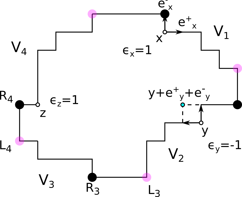
Figure 8: Definition of the $V_{k}$, $k\in\{1,...4\}$ for a curve $\gamma^{N}\in\Omega^{N}_{\text{mic}}$. The black dots are the first vertices and the light dots the last vertices of each $V_{k}$. Three points are marked by empty circles, with the corresponding value of $\varepsilon_{\cdot}(\gamma^{N})$. The block that is deleted if $y$ is flipped is materialised by dashed lines, and the two arrows with origin $y$ correspond to ${\bf e}^{+}_{y}$ (left arrow) and ${\bf e}^{-}_{y}$ (up arrow).

$$\frac{1}{N}\mathcal{B}_{t}(\gamma^{N}) =\frac{1}{2N}\sum_{x\in V(\gamma^{N})}c_{x}(\gamma^{N})H_{t}(x)^{2}+\sum_{x\in V(\gamma^{N})}c_{x}(\gamma^{N})\varepsilon_{x}(\gamma^{N})H_{t}(x)$$

$$\quad+\frac{1}{2}\sum_{x\in V(\gamma^{N})}c_{x}(\gamma^{N})\varepsilon_{x}(\gamma^{N})\big{(}\partial_{{\bf e}^{-}_{x}}+\partial_{{\bf e}^{+}_{x}}\big{)}H_{t}(x)+\frac{\eta^{\prime}(H_{t})|\gamma^{N}|}{N^{2}},$$ (3.37)

where $\eta^{\prime}(H_{t})$ is bounded by a constant depending on $H_{t}$ and its derivatives. The first and third sums above are bounded by $|V(\gamma^{N})|/N$, which is typically bounded with $N$ for nice curves in $\mathcal{E}$. At first glance however, the second sum in the first line of (3.37) appears to be of order $|V(\gamma^{N})|$. To prove that it is in fact also of order 1 in $N$, we shall use the link with the SSEP in each region of $\gamma^{N}$ to perform integration by parts. Let us more generally set out how to compute (3.37).

To compute (3.37) and interpret the summand in terms of tangent vectors as in Lemma 3.7, the idea is to split $V(\gamma^{N})$ into four pieces, essentially corresponding to the four regions of $\gamma^{N}$. This is done to map the dynamics inside each region onto an exclusion process as in Section 2.4. Through this mapping, $c_{x}(\gamma^{N}),\varepsilon_{x}(\gamma^{N})$ can be expressed only in terms of the local edge states $\xi_{x+{\bf e}^{-}_{x}},\xi_{x}$ inside each region. Mirroring similar results for the SSEP, these $\xi_{\cdot}$ are then replaced by local averages thanks to a replacement lemma-type result, Lemma 3.8. Inside each region, these averages are then rewritten as components of the microscopic tangent vector ${\bf t}^{\varepsilon N}_{\cdot}$ (defined in (3.6)), which allows one to cover a region-independent expression.

For $1\leq k\leq 4$, consider thus the set $V_{k}(\gamma^{N})\subset V(\gamma^{N})$ containing all vertices from $R_{k}$ to $L_{k+1}$ (comprised), see Figure 8, with $L_{k+1}:=L_{1}$ if $k=4$. Then $V_{k}$ is included in region $k$ of $\gamma^{N}$, and:

$$V(\gamma^{N})=\bigcup_{k=1}^{4}V_{k}(\gamma^{N})\cup\bigcup_{k=1}^{4}P_{k}(\gamma^{N}).$$ (3.38)

In the following, we often abbreviate $V_{k}(\gamma^{N})$ as $V_{k}$, and similarly $R_{k}(\gamma^{N}),L_{k}(\gamma^{N})$ as $R_{k},L_{k}$ for each $1\leq k\leq 4$.
Inside each $V_{k}$, the quantity $c_{x}(\gamma^{N})\varepsilon_{x}(\gamma^{N})$ can be expressed in terms of the $\xi$’s:

$$2c_{x}(\gamma^{N})\varepsilon_{x}(\gamma^{N})=\begin{cases}\xi_{x+{\bf e}^{-}_{x}}-\xi_{x}\quad\text{if }x\in V_{1}\cup V_{3},\\ \xi_{x}-\xi_{x+{\bf e}^{-}_{x}}\quad\text{if }x\in V_{2}\cup V_{4}.\end{cases}$$ (3.39)

Moreover, $c_{x}(\gamma^{N})=0$ for each $x\in\cup_{k}P_{k}(\gamma^{N})\setminus\{R_{k}(\gamma^{N}),L_{k}(\gamma^{N})\}$, so that the sums in (3.37) reduce to sums on $V_{k}$, $1\leq k\leq 4$. With this splitting along the $V_{k}$, (3.37) becomes:

$$\frac{1}{N}\mathcal{B}_{t}(\gamma^{N})=\frac{1}{2N}\sum_{x\in V(\gamma^{N})}c_{x}(\gamma^{N})H_{t}(x)^{2}+\sum_{k=1}^{4}B_{t}^{k}+\sum_{k=1}^{4}\tilde{B}_{t}^{k}+\frac{\eta^{\prime}(H_{t})|\gamma^{N}|}{N^{2}},$$ (3.40)

where:

$$B_{t}^{k}:=\sum_{x\in V_{k}}c_{x}(\gamma^{N})\varepsilon_{x}(\gamma^{N})H_{t}(x),\quad\tilde{B}_{t}^{k}:=\frac{1}{2}\sum_{x\in V_{k}}c_{x}(\gamma^{N})\varepsilon_{x}(\gamma^{N})\big{(}\partial_{{\bf e}^{-}_{x}}+\partial_{{\bf e}^{+}_{x}}\big{)}H_{t}(x).$$ (3.41)

Let us first treat the sums $B^{k}_{t},\tilde{B}^{k}_{t}$ for $1\leq k\leq 4$, involving $\varepsilon_{x}(\gamma^{N})$.

1) $B_{t}^{k}$ terms. Using Equation (3.39), one has e.g. for $k=1$:

$$B_{t}^{1} =\sum_{x\in V_{1}(\gamma^{N})}c_{x}(\gamma^{N})\varepsilon_{x}(\gamma^{N})H_{t}(x)=\frac{1}{2}\sum_{x\in V_{1}(\gamma^{N})}H_{t}(x)(\xi_{x+{\bf e}^{-}_{x}}-\xi_{x})$$

$$=\frac{1}{4}\sum_{x\in V_{1}(\gamma^{N})}H_{t}(x)\big{[}\xi_{x+{\bf e}^{-}_{x}}-\xi_{x}+(1-\xi_{x})-(1-\xi_{x+{\bf e}^{-}_{x}})\big{]}.$$ (3.42)

The passage from first to second line is nothing more than a symmetrisation of the expression.
By definition, the edge with right extremity $R_{1}$, corresponding to $[R_{1}+{\bf e}^{-}_{R_{1}},R_{1}]$, is always horizontal: $1-\xi_{R_{1}+{\bf e}^{-}_{R_{1}}}=1$. On the other hand, $V_{1}$, corresponding to all vertices between $R_{1}$ and $L_{2}$, ends at $L_{2}$ by assumption; and $\xi_{L_{2}}=1$ by definition of $L_{2}$. Integrating (3.42) by parts, some of the boundary term thus vanish, whence:

$$B_{t}^{1} =-\frac{1}{4}\big{(}H_{t}(R_{1})+H_{t}(L_{2})\big{)}$$

$$\hskip 56.9055pt+\frac{1}{4}\sum_{x\in V_{1}\setminus\{R_{1},L_{2}\}}\bigg{[}\xi_{x}\Big{[}H_{t}(x+{\bf e}^{+}_{x})-H_{t}(x)\Big{]}-(1-\xi_{x})\Big{[}H_{t}(x+{\bf e}^{+}_{x})-H_{t}(x)\Big{]}\bigg{]}$$

$$=-\frac{1}{4}\big{(}H_{t}(R_{1})+H_{t}(L_{2})\big{)}$$

$$\hskip 56.9055pt+\frac{1}{4}\sum_{x\in V_{1}\setminus\{R_{1},L_{2}\}}\big{[}\xi_{x}\partial_{{\bf e}^{+}_{x}}H_{t}(x)-(1-\xi_{x})\partial_{{\bf e}^{+}_{x}}H_{t}(x)\big{]}+\eta^{1}(H_{t},\gamma^{N}),$$ (3.43)

with $\eta_{t}^{1}(H_{t},\gamma^{N})$ an error term bounded by:

$$\big{|}\eta^{1}(H_{t},\gamma^{N})\big{|}\leq\frac{\|\nabla^{2}H_{t}\|_{\infty}|V_{1}(\gamma^{N})|}{4N^{2}}.$$ (3.44)

Recall that due to the fact that ${\bf e}^{\pm}_{x}$ has norm $1/N$, the sum in (3.43) is bounded by $C(H)|V_{1}|/N$ for some $C(H)>0$, which is one factor of $1/N$ smaller than the expression (3.41) of $B^{1}_{t}$ as desired.
The other $V_{k}$, $2\leq k\leq 4$ are treated similarly, with signs depending on the region due to both (3.39) and the fact that $N{\bf e}^{+}_{x}$ takes the values $\pm{\bf b}_{1},\pm{\bf b}_{2}$ as the region varies. The point is now, from the expression of each $B_{t}^{k}$, to obtain an expression independent of the region of $\gamma^{N}$. To do so, introduce region-dependent signs $\sigma_{1},\sigma_{2}$:

$$\sigma_{1}:=\begin{cases}1\quad&\text{if }x\in V_{1}\cup V_{4}\\ -1\quad&\text{if }x\in V_{2}\cup V_{3}\end{cases},\quad\sigma_{2}:=\begin{cases}-1\quad&\text{if }x\in V_{1}\cup V_{2}\\ 1\quad&\text{if }x\in V_{3}\cup V_{4}\end{cases}.$$ (3.45)

The idea behind (3.45) is that $(\sigma_{1},\sigma_{2})$ is "the direction of the tangent vector to a curve" in each region, in the spirit of Property 2.1. For instance, in the first region, the tangent vector can be either ${\bf b}_{1}$ or $-{\bf b}_{2}$, and $(\sigma_{1},\sigma_{2})=(1,-1)$. In region $2$, $(\sigma_{1},\sigma_{2})=(-1,-1)$, etc. One can then check that:

$$\forall x\in V(\gamma^{N}),\qquad N{\bf e}^{+}_{x}=(1-\xi_{x})\sigma_{1}{\bf b}_{1}+\xi_{x}\sigma_{2}{\bf b}_{2}.$$ (3.46)

Compare with ${\bf m}(x)$ in Definition 3.1, which gives "the direction of the inwards normal" in the region $x$ belongs to:

$${\bf m}(x)=-(-\sigma_{2},\sigma_{1})=(\sigma_{2},-\sigma_{1})=\sigma_{2}{\bf b}_{1}-\sigma_{1}{\bf b}_{2}.$$ (3.47)

With Definition 3.45 and the error bound (3.44), recalling also from (3.34) differentiating along ${\bf e}^{+}_{x}$ incurs a factor $1/N$ compared to differentiating with respect to ${\bf b}_{1}$ or ${\bf b}_{2}$, $B^{1}_{t}$ can be written as:

$$B^{1}_{t} =-\frac{1}{4}\big{(}H_{t}(R_{1})+H_{t}(L_{2})\big{)}$$

$$\qquad+\frac{1}{4N}\sum_{x\in V_{1}\setminus\{R_{1},L_{2}\}}\Big{(}-\xi_{x}\sigma_{1}\partial_{2}+(1-\xi_{x})\sigma_{2}\partial_{1}\Big{)}H_{t}(x)+\eta^{1}(H_{t},\gamma^{N}).$$ (3.48)

Recalling the sign change (3.39) between regions, one can check that the expression of the last summand is independent from the region, thus:

$$\sum_{k=1}^{4}B_{t}^{k} =-\frac{1}{4}\sum_{k=1}^{4}\big{[}H_{t}(R_{k}(\gamma^{N}))+H_{t}(L_{k}(\gamma^{N}))\big{]}$$

$$\qquad+\frac{1}{4N}\sum_{x\in V(\gamma^{N})\setminus\cup_{k}P_{k}(\gamma^{N})}\Big{(}-\xi_{x}\sigma_{1}\partial_{2}+(1-\xi_{x})\sigma_{2}\partial_{1}\Big{)}H_{t}(x)+\sum_{k=1}^{4}\eta^{k}(H_{t},\gamma^{N}).$$ (3.49)

2) $\tilde{B}^{k}_{t}$ terms (defined in (3.41)). Recall that $\varepsilon_{x}(\gamma^{N})$ is defined in (3.33). The key observation is the following: for $x\in V(\gamma^{N})$, if $c_{x}(\gamma^{N})\neq 0$, then $\varepsilon_{x}(\gamma^{N})(\partial_{{\bf e}^{+}_{x}}+\partial_{{\bf e}^{-}_{x}})$ is the same whether flipping $x$ corresponds to adding or deleting a block, and it only depends on the region of the curve. Indeed, recall Definition (3.45) of $\sigma_{1},\sigma_{2}$. Using ${\bf e}^{-}_{x}=-{\bf e}^{+}_{x+{\bf e}^{-}_{x}}$ (see Figure 8) and the expression (3.46) of ${\bf e}^{+}_{x}$, one has:

$$\partial_{{\bf e}^{-}_{x}}+\partial_{{\bf e}^{+}_{x}}=\big{(}\xi_{x+{\bf e}^{-}_{x}}-\xi_{x}\big{)}\Big{(}\frac{\sigma_{1}}{N}\partial_{1}-\frac{\sigma_{2}}{N}\partial_{2}\Big{)}.$$ (3.50)

Using the expression (3.39) for $c_{x}(\gamma^{N})\varepsilon_{x}(\gamma^{N})$, elementary manipulations then yield:

$$\forall x\in V(\gamma^{N}),\qquad c_{x}(\gamma^{N})\varepsilon_{x}(\gamma^{N}) (\partial_{{\bf e}^{+}_{x}}+\partial_{{\bf e}^{-}_{x}})$$

$$\quad=\frac{c_{x}(\gamma^{N})}{N}\Big{(}-\sigma_{2}\partial_{1}+\sigma_{1}\partial_{2}\Big{)}=-\frac{c_{x}(\gamma^{N})}{N}{\bf m}(x)\cdot\nabla,$$ (3.51)

with ${\bf m}(x)$ the sign vector of Definition 3.1. As a result:

$$\sum_{k=1}^{4}\tilde{B}^{k}_{t}(\gamma^{N})=-\frac{1}{2N}\sum_{x\in V(\gamma^{N})\setminus\cup_{k}P_{k}(\gamma^{N})}c_{x}(\gamma^{N}){\bf m}(x)\cdot\nabla H_{t}(x).\vskip 12.0pt plus 4.0pt minus 4.0pt$$ (3.52)

To obtain the expression in Lemma 3.7 from (3.40)-(3.49)-(3.52), fix $\varepsilon>0$ and let us now replace $\xi_{\cdot}$ and $c_{\cdot}(\gamma^{N})$ by local averages on boxes containing order $\varepsilon N$ vertices; then express them in terms of the microscopic tangent vector ${\bf t}^{\varepsilon N}_{\cdot}$ defined in (3.6). Let $V^{\varepsilon}(\gamma^{N})$ be the subset of $V(\gamma^{N})$ made of vertices at $1$-distance at least $\varepsilon$ from each pole. At this point, the bulk term $\mathcal{B}_{t}$ can be written as:

$$\frac{1}{N}\mathcal{B}_{t}(\gamma^{N}) =\frac{1}{2N}\sum_{x\in V^{\varepsilon}(\gamma^{N})}c_{x}(\gamma^{N})H_{t}(x)^{2}-\frac{1}{4}\sum_{k=1}^{4}\big{[}H_{t}(R_{k}(\gamma^{N}))+H_{t}(L_{k}(\gamma^{N}))\big{]}$$

$$\qquad+\frac{1}{4N}\sum_{x\in V^{\varepsilon}(\gamma^{N})}\Big{(}-\xi_{x}\sigma_{1}\partial_{2}+(1-\xi_{x})\sigma_{2}\partial_{1}\Big{)}H_{t}(x)$$ (3.53)

$$\qquad-\frac{1}{2N}\sum_{x\in V^{\varepsilon}(\gamma^{N})}c_{x}(\gamma^{N}){\bf m}(x)\cdot\nabla H_{t}(x)+\eta(H_{t},\varepsilon,\gamma^{N}),$$

where $\eta(H_{t},\varepsilon,\gamma^{N})$ satisfies, for some constant $C(H)>0$ independent of $\gamma^{N}$:

$$\Big{|}\eta(H_{t},\varepsilon,\gamma^{N})-\frac{\eta^{\prime}(H_{t})|\gamma^{N}|}{N^{2}}-\sum_{k=1}^{4}\eta^{k}(H_{t},\gamma^{N})\Big{|}\leq C(H)\varepsilon.$$ (3.54)

We now replace $c_{\cdot}(\gamma^{N}),\xi_{\cdot}$ by local averages. For $\xi_{\cdot}$, an integration by parts and the smoothness of $H_{t}$ yield the existence of an error term $\omega^{\nabla H_{t}}(\varepsilon,\gamma^{N})$ such that:

$$\frac{1}{4N}\sum_{x\in V^{\varepsilon}(\gamma^{N})}\Big{(}-\xi_{x}\sigma_{1}\partial_{2}+(1-\xi_{x})\sigma_{2}\partial_{1}\Big{)}H_{t}(x)$$

$$\hskip 85.35826pt=\frac{1}{4N}\sum_{x\in V^{\varepsilon N}(\gamma^{N})}\Big{(}-\xi^{\varepsilon N}_{x}\sigma_{1}\partial_{2}+(1-\xi_{x}^{\varepsilon N})\sigma_{2}\partial_{1}\Big{)}H_{t}(x)+\omega^{\nabla H_{t}}(\varepsilon,\gamma^{N}),$$ (3.55)

with, for a constant $C(H_{t})>0$ involving $\nabla^{2}H_{t}$ but independent of $\gamma^{N}$:

$$|\omega^{\nabla H_{t}}(\varepsilon,\gamma^{N})\big{|}\leq C(H_{t})\varepsilon.$$ (3.56)

Replacing $c_{\cdot}(\gamma^{N})$ by a local average is much more involved. It is the content of a so-called replacement lemma, stated below and proven in Appendix A.

Lemma 3.8 (Replacement lemma).

Let $G:\mathbb{R}_{+}\times\mathbb{R}^{2}\rightarrow\mathbb{R}$ be bounded, $A,\varepsilon>0$ and $1\leq k\leq 4$. Define $W_{\varepsilon N}^{G,k}(t,\cdot)$ for $t\geq 0$ by:

$$W_{\varepsilon N}^{G,k}(t,\tilde{\gamma}^{N}):=\frac{1}{N}\sum_{x\in V_{k}(\tilde{\gamma}^{N})}G(t,x)\bigg{[}c_{x}(\tilde{\gamma}^{N})-\xi^{\varepsilon N}_{x}\big{(}1-\xi^{\varepsilon N}_{x}\big{)}\bigg{]},\quad\tilde{\gamma}^{N}\in\Omega^{N}_{\text{mic}}.$$ (3.57)

Then, for each $\delta>0$, the following super-exponential estimate holds:

$$\limsup_{\varepsilon\rightarrow 0}\limsup_{N\rightarrow\infty}\frac{1}{N}\log\mathbb{P}_{\beta,H}^{N}\Big{(}(\gamma^{N}_{t})_{t\leq T}\in E([0,T],\mathcal{E})\cap\big{\{}\sup_{t\leq T}|\gamma^{N}_{t}|\leq A\big{\}};$$

$$\hskip 42.67912pt\bigg{|}\int_{0}^{T}W_{\varepsilon N}^{G,k}(t,\gamma^{N}_{t})dt\bigg{|}>\delta\Big{)}=-\infty.$$ (3.58)

Using Lemma 3.8, we are going to conclude the proof of Lemma 3.7. Define, for each bounded function $G$:

$$B_{G}(\delta,\varepsilon)=\bigg{\{}(\gamma^{N}_{t})_{t\leq T}\subset\Omega^{N}_{\text{mic}}:\forall 1\leq k\leq 4,\ \bigg{|}\int_{0}^{T}W_{\varepsilon N}^{G,k}(t,\gamma^{N}_{t})dt\bigg{|}\leq\delta/4\bigg{\}}.$$ (3.59)

By Lemma 3.8, for each $A,\delta>0$, one has:

$$\limsup_{\varepsilon\rightarrow 0}\limsup_{N\rightarrow\infty}\frac{1}{N}\log\mathbb{P}^{N}_{\beta,H}\Big{(}B_{G}(\delta,\varepsilon)^{c}\cap E([0,T],\mathcal{E})\cap\Big{\{}\sup_{t\leq T}|\gamma^{N}_{t}|\leq A\Big{\}}\Big{)}=-\infty.$$ (3.60)

Define then the set controlling the error terms:

$$Z_{B}=Z_{B}(H,\delta,\varepsilon):=B_{\partial_{1}H}(\delta,\varepsilon)\cap B_{\partial_{2}H}(\delta,\varepsilon)\cap B_{H^{2}}(\delta,\varepsilon).$$ (3.61)

We may now write the bulk term $\mathcal{B}_{t}$ (recall (3.53)) as:

$$\frac{1}{N}\mathcal{B}_{t}(\gamma^{N}) =\frac{1}{2N}\sum_{x\in V^{\varepsilon}(\gamma^{N})}\xi_{x}^{\varepsilon N}\big{(}1-\xi^{\varepsilon N}_{x}\big{)}H_{t}(x)^{2}-\frac{1}{4}\sum_{k=1}^{4}\big{[}H_{t}(R_{k}(\gamma^{N}))+H_{t}(L_{k}(\gamma^{N}))\big{]}$$

$$\qquad+\frac{1}{4N}\sum_{x\in V^{\varepsilon}(\gamma^{N})}\Big{(}-\xi^{\varepsilon N}_{x}\sigma_{1}\partial_{2}+(1-\xi^{\varepsilon N}_{x})\sigma_{2}\partial_{1}\Big{)}H_{t}(x)$$ (3.62)

$$\qquad-\frac{1}{2N}\sum_{x\in V^{\varepsilon}(\gamma^{N})}\xi_{x}^{\varepsilon N}\big{(}1-\xi^{\varepsilon N}_{x}\big{)}{\bf m}(x)\cdot\nabla H_{t}(x)+\omega_{B}(H_{t},\delta,\varepsilon,\gamma^{N}),$$

where $\omega_{B}(H_{t},\delta,\varepsilon,\gamma^{N})$ is defined, with a slight abuse of notation, by:

$$\omega_{B}(H_{t},\delta,\varepsilon,\gamma^{N}):=\eta(H_{t},\varepsilon,\gamma^{N})+\omega^{\nabla H_{t}}(\varepsilon,\gamma^{N})+\sum_{k=1}^{4}\Big{[}W_{\varepsilon N}^{{\bf m}\cdot\nabla H,k}(t,\gamma^{N})+W_{\varepsilon N}^{H^{2},k}(t,\gamma^{N})\Big{]}.$$ (3.63)

In particular, for microscopic trajectories $(\gamma^{N}_{t})_{t\leq T}\in Z_{B}\cap E([0,T],\mathcal{E})$, there is a constant $C(H)>0$ such that:

$$\Big{|}\int_{0}^{T}\omega_{B}(H_{t},\delta,\varepsilon,\gamma^{N}_{t})dt\Big{|}\leq 2\delta+C(H)\Big{(}\varepsilon T+\frac{1}{N^{2}}\int_{0}^{T}|\gamma^{N}_{t}|dt\Big{)}.$$ (3.64)

With the above estimate of $\omega_{B}(\cdot)$ and the expression (3.62) of $\mathcal{B}_{t}$, we see that the proof of Lemma 3.7 now reduces to the third step in the program outlined below (3.37), i.e. the interpretation of $\xi^{\varepsilon N}_{x}$ and ${\bf m}(x)\cdot\nabla$ in terms of components of the microscopic tangent vector ${\bf t}^{\varepsilon N}_{x}$, which we now perform.

Recall from (3.6) the following identity: for $\gamma^{N}\in\Omega^{N}_{\text{mic}}\cap\mathcal{E}$ and $x\in V(\gamma^{N})$,

$$|{\bf t}^{\varepsilon N}_{x}\cdot{\bf b}_{2}|=\xi^{\varepsilon N}_{x}=1-|{\bf t}^{\varepsilon N}_{x}\cdot{\bf b}_{1}|.$$ (3.65)

As a result:

$$\frac{1}{2N}\sum_{x\in V^{\varepsilon}(\gamma^{N})}\xi_{x}^{\varepsilon N}\big{(}1-\xi^{\varepsilon N}_{x}\big{)}H_{t}(x)^{2}=\frac{1}{2N}\sum_{x\in V^{\varepsilon}(\gamma^{N})}|{\bf t}^{\varepsilon N}_{x}\cdot{\bf b}_{1}||{\bf t}^{\varepsilon N}_{x}\cdot{\bf b}_{2}|H_{t}(x)^{2}.$$ (3.66)

To establish the expression (3.30), we therefore only need to prove:

$$\frac{1}{4N}\sum_{x\in V^{\varepsilon}(\gamma^{N})}\Big{(}-\xi^{\varepsilon N}_{x}\sigma_{1}\partial_{2}+(1-\xi^{\varepsilon N}_{x})\sigma_{2}\partial_{1}\Big{)}H_{t}(x)$$ (3.67)

$$-\frac{1}{2N}\sum_{x\in V^{\varepsilon}(\gamma^{N})}\xi_{x}^{\varepsilon N}\big{(}1-\xi^{\varepsilon N}_{x}\big{)}{\bf m}(x)\cdot\nabla H_{t}(x)=\frac{1}{4N}\sum_{x\in V^{\varepsilon}(\gamma^{N})}\big{[}{\bf t}^{\varepsilon N}_{x}\cdot{\bf m}(x)\big{]}{\bf t}_{x}^{\varepsilon N}\cdot\nabla H_{t}(x).$$

To do so, we use the following shorthand notations:

$${\bf t}^{\varepsilon}:={\bf t}^{\varepsilon N}_{x},\qquad{\bf t}^{\varepsilon}_{i}:={\bf t}^{\varepsilon N}_{x}\cdot{\bf b}_{i},\quad i\in\{1,2\}.$$ (3.68)

Recalling that ${\bf m}(x)=(\sigma_{2},-\sigma_{1})$, the left-hand side of (3.67) then reads:

$$\frac{1}{4N} \sum_{x\in V^{\varepsilon}(\gamma^{N})}\Big{[}\big{(}-|{\bf t}^{\varepsilon}_{2}|\sigma_{1}+2|{\bf t}^{\varepsilon}_{1}||{\bf t}^{\varepsilon}_{2}|\sigma_{1}\big{)}\partial_{2}+\big{(}|{\bf t}^{\varepsilon}_{1}|\sigma_{2}-2|{\bf t}^{\varepsilon}_{1}||{\bf t}^{\varepsilon}_{2}|\sigma_{2}\big{)}\partial_{1}\Big{]}H_{t}(x)$$

$$\qquad=\frac{1}{4N}\sum_{x\in V^{\varepsilon}(\gamma^{N})}\Big{[}\sigma_{1}|{\bf t}^{\varepsilon}_{2}|\big{(}-1+2|{\bf t}^{\varepsilon}_{1}|\big{)}\partial_{2}+\sigma_{2}|{\bf t}^{\varepsilon}_{1}|\big{(}1-2|{\bf t}^{\varepsilon}_{2}|\sigma_{2}\big{)}\partial_{1}\Big{]}H_{t}(x)$$

$$\qquad=\frac{1}{4N}\sum_{x\in V^{\varepsilon}(\gamma^{N})}\Big{[}\sigma_{1}|{\bf t}^{\varepsilon}_{2}|\big{(}|{\bf t}^{\varepsilon}_{1}|-|{\bf t}^{\varepsilon}_{2}|\big{)}\partial_{2}+\sigma_{2}|{\bf t}^{\varepsilon}_{1}|\big{(}|{\bf t}^{\varepsilon}_{1}|-|{\bf t}^{\varepsilon}_{2}|\big{)}\partial_{1}\Big{]}H_{t}(x).$$ (3.69)

To obtain the third line, we used $|{\bf t}^{\varepsilon}_{1}|+|{\bf t}^{\varepsilon}_{2}|=1$ as recalled in (3.65).
Recall from (3.45) the definition of $(\sigma_{1},\sigma_{2})$, and that $V^{\varepsilon}(\gamma^{N})\subset V(\gamma^{N})$ is the set of vertices at $1$-distance at least $\varepsilon$ to the poles to obtain:

$$\forall x\in V^{\varepsilon}(\gamma^{N}),\qquad|{\bf t}^{\varepsilon}_{1}|:=|{\bf t}^{\varepsilon N}_{x}\cdot{\bf b}_{1}|=\sigma_{1}{\bf t}^{\varepsilon}_{1},\qquad|{\bf t}^{\varepsilon}_{2}|:=|{\bf t}^{\varepsilon N}_{x}\cdot{\bf b}_{2}|=\sigma_{2}{\bf t}^{\varepsilon}_{2}.$$ (3.70)

This is because all points in the $1$-norm ball $B_{1}(x,\varepsilon)$ around $x$ are in the same region of $\gamma^{N}$ when $x\in V^{\varepsilon}(\gamma^{N})$, thus $\sigma_{1},\sigma_{2}$ are constant on $V(\gamma^{N})\cap B_{1}(x,\varepsilon)$. As a result, the last line of (3.69) is equal to:

$$\frac{1}{4N}\sum_{x\in V^{\varepsilon}(\gamma^{N})}\Big{[}\sigma_{1}\sigma_{2}{\bf t}^{\varepsilon}_{2}\big{(}\sigma_{1}{\bf t}^{\varepsilon}_{1}-\sigma_{2}{\bf t}^{\varepsilon}_{2}\big{)}\partial_{2}+\sigma_{2}\sigma_{1}{\bf t}^{\varepsilon}_{1}\big{(}\sigma_{1}{\bf t}^{\varepsilon}_{1}-\sigma_{2}{\bf t}^{\varepsilon}_{2}\big{)}\partial_{1}\Big{]}H_{t}(x)$$

$$\qquad=\frac{1}{4N}\sum_{x\in V^{\varepsilon}(\gamma^{N})}\big{[}\sigma_{2}{\bf t}^{\varepsilon}_{1}-\sigma_{1}{\bf t}^{\varepsilon}_{2}\big{]}\big{[}{\bf t}^{\varepsilon}_{1}\partial_{1}+{\bf t}^{\varepsilon}_{2}\partial_{2}\big{]}H_{t}(x)$$

$$\qquad=\frac{1}{4N}\sum_{x\in V^{\varepsilon}(\gamma^{N})}\big{[}{\bf t}^{\varepsilon}\cdot{\bf m}(x)\big{]}{\bf t}^{\varepsilon}\cdot\nabla H_{t}(x).$$ (3.71)

This concludes the proof of Lemma 3.7. Indeed, the set $Z_{B}$ was defined in (3.61). Equation (3.30) then follows from the expression (3.62) with the two identities (3.66)-(3.71). ∎

Lemmas 3.3 and 3.7 yield the statement of Proposition 3.2, setting:

$$\tilde{\omega}(H_{t},\delta,\varepsilon,\gamma^{N}):=\omega_{B}(H_{t},\delta,\varepsilon,\gamma^{N})+\omega_{P}(H_{t},\delta,\gamma^{N}),\qquad\gamma^{N}\in\Omega^{N}_{\text{mic}},$$ (3.72)

as well as (recall (3.27)-(3.61)):

$$\tilde{Z}:=Z_{B}\cap Z_{P},$$ (3.73)

and recalling the normalisation ${\bf t}^{\varepsilon N}_{x}=\mathsf{v}^{\varepsilon N}_{x}{\bf T}^{\varepsilon N}_{x}$ in (3.8).

Let us conclude the section with a useful bound on the Radon-Nikodym derivative, obtained as a consequence of the computations in the proofs of Lemmas 3.3-3.7. We stress that the result below does not require an estimate of the error terms, and is therefore valid for any trajectory in $E([0,T],\mathcal{E})$.

Corollary 3.9.

Let $H\in\mathcal{C}$ be a bias. Recall from (4.1) the definition of the Radon-Nikodym derivative $D^{N}_{\beta,H}:=d\mathbb{P}^{N}_{\beta,H}/d\mathbb{P}^{N}_{\beta}$. There is a constant $C(H)>0$ such that, for each $T>0$ and each trajectory $(\gamma^{N}_{t})_{t\leq T}$ with values in $\Omega^{N}_{\text{mic}}\cap\mathcal{E}$:

$$\exp\Big{[}-C(H)N-C(H)N\int_{0}^{T}|\gamma^{N}_{t}|dt\Big{]}\leq D^{N}_{\beta,H}((\gamma^{N}_{t})_{t\leq T})\leq\exp\Big{[}C(H)N+C(H)N\int_{0}^{T}|\gamma^{N}_{t}|dt\Big{]}.$$

The same bounds hold for $\exp\big{[}\big{|}\int_{0}^{T}e^{N\big{<}\Gamma^{N}_{t},H\big{>}}N^{2}\mathcal{L}_{\beta}e^{N\big{<}\Gamma^{N}_{t},H\big{>}}dt\big{|}\big{]}$, without the factors $e^{\pm C(H)N}$.

3.2.3 From microscopic sums to line integrals

The objective of this section is to turn the expression of Proposition 3.2 into an $N$-independent object, with nice continuity properties with respect to the topology on $E([0,T],\mathcal{E})$ (see (2.39)). The statement of the result requires some notations, which we introduce together with an explanation of the difficulties.

In Proposition 3.2, for each $T>0$, we find a set $\tilde{Z}$ of trajectories such that, if $(\gamma^{N}_{t})_{t\leq T}\in\tilde{Z}\cap E([0,T],\mathcal{E})$, the action of the generator in the Radon-Nikodym derivative (4.1) contains terms of the form:

$$\int_{0}^{T}\frac{1}{N}\sum_{x\in V(\gamma^{N}_{t})}f(t,\gamma^{N}_{t},x)dt,$$ (3.74)

with $f$ a bounded mapping that depends on a neighbourhood of the vertex $x$ inside $\gamma^{N}_{t}$ at each time $t\in[0,T]$. To make sense of such an expression when $N$ is large, we would like:

• To prove that there is a sufficiently big set $Z\subset\tilde{Z}$ on which microscopic curves have length of order $N$ at each time, so that the sum in (3.74) is typically of order $1$ when $N$ is large, and on this set the Replacement Lemma 3.8 is typical.

• To then prove that this discrete sum can be seen as the discretisation of a suitable line integral on $\gamma^{N}_{t}$ at each time $t\in[0,T]$. Informally, this line integral should have the same continuity property as the discrete version: if $\gamma^{N}\in\Omega^{N}_{\text{mic}}\cap\mathcal{E}$, a small change of $\gamma^{N}$ in Hausdorff distance should correspond to a small change in the corresponding line integral.

The first point is treated in the following lemma, proven in Section 5.2.1.

Lemma 3.10.

Let $\beta>1$. For each $T^{\prime}>0$, there is $C(\beta,H,T^{\prime})>0$ such that:

$$\forall A>0,\qquad\limsup_{N\rightarrow\infty}\mathbb{P}^{N}_{\beta}\Big{(}\sup_{t\leq T^{\prime}}|\gamma^{N}_{t}|\geq A\Big{)}\leq-C(\beta,H,T^{\prime})A.$$ (3.75)

It will thus be enough to define $Z$ as the intersection of $\tilde{Z}$ and a set where the length is well-controlled, as done below in (3.89).

Let us now focus on the second point. Let $\tilde{\gamma}\in\Omega\cap\mathcal{E}$ be a Lipschitz Jordan curve. Let $(\tilde{\gamma}(u))_{u\in[0,1)}$ denote a parametrisation of $\tilde{\gamma}$. The line integral of a continuous $f:\mathbb{R}^{2}\rightarrow\mathbb{R}$ on $\tilde{\gamma}$ reads, by definition:

$$\int_{\tilde{\gamma}}fds:=\int_{0}^{1}f(\tilde{\gamma}(u))\|\tilde{\gamma}^{\prime}(u)\|_{2}du,$$ (3.76)

where $s$ denotes the arclength coordinate on $\tilde{\gamma}$. Assume that $\tilde{\gamma}=\gamma^{N}$ with $\gamma^{N}\in\Omega^{N}_{\text{mic}}\cap\mathcal{E}$. In this case, $\tilde{\gamma}^{\prime}(u)$ is proportional to either ${\bf b}_{1}$ or ${\bf b}_{2}$, and the line integral reads:

$$\int_{\tilde{\gamma}}fds=\sum_{x\in V(\gamma^{N})}f(x)[s(x+{\bf e}^{+}_{x})-s(x)]=\frac{1}{N}\sum_{x\in V(\gamma^{N})}f(x).$$ (3.77)

For a microscopic curve, the discrete sums of Proposition 3.2 could therefore be replaced with line integrals without loss of information.

The problem with (3.77), however, is that, loosely speaking, the right-hand side is continuous in Hausdorff distance, but the left-hand side is not. Indeed, informally, the right-hand side is continuous in Hausdorff distance: adding or deleting one block to the droplet associated with $\gamma^{N}$ does not change the sum much. To understand why, however, the left-hand side does not preserve this continuity, consider the simplest case $f\equiv 1$. Recall that $|\gamma^{N}|$ is the length of $\gamma^{N}$ in 1-norm, and let $|\gamma^{N}|_{2}$ be its length in $2$-norm. Then:

$$|\gamma^{N}|_{2}:=\int_{\gamma^{N}}1ds=\frac{1}{N}\sum_{x\in V(\gamma^{N})}1=|\gamma^{N}|,$$ (3.78)

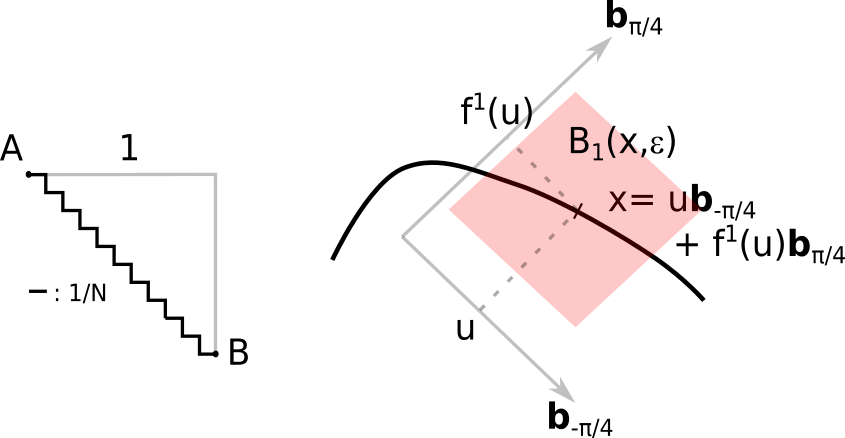
Figure 9: Left figure: a lattice path on $(N^{-1}\mathbb{Z})^{2}$ between the two extremities $A$ and $B$ of the unit square. The path has length $2$ in both one- and two-norms. It converges in Hausdorff distance to the diagonal of the unit-square, which has 2-norm length $\sqrt{2}$.
Right figure: neighbourhood of a point $x$ at distance at least $\varepsilon$ from the poles in one-norm. In the ball $B_{1}(x,\varepsilon)$, the curve corresponds to the graph of a function $f^{1}$ in the reference frame $({\bf b}_{-\pi/4},{\bf b}_{\pi/4})$.

It is easy to see that the length $|\cdot|$ in one-norm (recall (2.6)) is continuous in Hausdorff distance, using e.g.:

$$|\gamma|=2\big{[}L_{1}(\gamma)-L_{3}(\gamma)\big{]}\cdot{\bf b}_{2}+2\big{[}L_{2}(\gamma)-L_{4}(\gamma)\big{]}\cdot{\bf b}_{1},\qquad\gamma\in\Omega.$$ (3.79)

The continuity of the above functionals is established in Lemma B.3. The length $|\cdot|_{2}$ in two-norm is however not continuous in Hausdorff distance. Indeed, assume that $(\gamma^{N})_{N}$ converges in Hausdorff distance to a curve $\gamma^{\infty}$, and suppose $\gamma^{\infty}$ is not a lattice path: $\gamma^{\infty}\notin\bigcup_{N}\Omega_{\text{mic}}^{N}$. Then $|\gamma^{\infty}|_{2}\neq|\gamma^{\infty}|$, see Figure 9. However if $|\cdot|_{2}$ were continuous, (3.78) would yield:

$$|\gamma^{\infty}|_{2}=\int_{\gamma^{\infty}}1ds=\lim_{N\rightarrow\infty}\frac{1}{N}\sum_{x\in V(\gamma^{N})}1=|\gamma^{\infty}|,$$ (3.80)

which is a contradiction. We claim that, to preserve continuity of the right-hand side of (3.77) in Hausdorff distance, it must be written in terms of the following line integral:

$$\frac{1}{N}\sum_{x\in V(\gamma^{N})}f(x)=\frac{1}{N}\sum_{x\in V(\gamma^{N})}f(x)\|{\bf T}_{x}\|_{1}=\int_{\gamma^{N}}f\mathsf{v}^{-1}ds,$$ (3.81)

where, for $x\in V(\gamma^{N})$, ${\bf T}_{x}$ is the unit vector in $\|\cdot\|_{2}$-norm, tangent to the edge $[x,x+{\bf e}^{+}_{x}]$. The quantity $\mathsf{v}$ is given by $\mathsf{v}^{-1}:=\|{\bf T}\|_{1}$, and plays the same role as the $\|\gamma^{\prime}(u)\|_{2}$ term in (3.77). Note that $\mathsf{v}$ is identically equal to $1$ for microscopic curves, for which ${\bf T}_{x}$ is either $\pm{\bf b}_{1}$ or $\pm{\bf b}_{2}$.
The claim that (3.81) is the correct way to write the discrete sums is a consequence of the proof of Proposition 4.1, and is established in Appendix B.2.2 where we prove that, for continuous $f:\mathbb{R}^{2}\rightarrow\mathbb{R}$:

$$\gamma\in\mathcal{E}\mapsto\int_{\gamma}f\mathsf{v}^{-1}ds\quad\text{is continuous in Hausdorff distance.}$$ (3.82)

The argument in Appendix B.2.2 is actually carried out only for the integrands appearing in Proposition 3.11, but could be generalised to the above setting.
Admitting the claim (3.82), we may recast the expression of Proposition 3.2 in terms of line integrals as follows. To do so, we need some notations. Let $\gamma\in\Omega$ be a macroscopic interface. For $\varepsilon>0$, let $\gamma(\varepsilon)$ denote all points of $\gamma$ at $1$-distance at least $\varepsilon$ from each poles, and let $x\in\gamma(\varepsilon)$. For definiteness, assume $x$ be in the first region of $\gamma$. By Property 2.1 of elements of $\Omega$, the portion $\gamma\cap B_{1}(x,\varepsilon)$ of $\gamma$ is the graph of a $1$-Lipschitz function $f^{1}$ in the reference frame $({\bf b}_{-\pi/4},{\bf b}_{\pi/4})$ (see Figure 9):

$$\gamma\cap B_{1}(x,\varepsilon)=\Big{\{}w{\bf b}_{-\pi/4}+f^{1}(w){\bf b}_{\pi/4}:w\in u+[-\varepsilon/\sqrt{2},\varepsilon/\sqrt{2}]\Big{\}},\quad u:=x\cdot{\bf b}_{-\pi/4}.$$ (3.83)

The curve $\gamma$ has well-defined tangent vector at almost every point as it is Lipschitz. Let ${\bf t}$ and ${\bf T}$ denote two different normalisations of the same tangent vector, so that:

$${\bf t}=\mathsf{v}{\bf T},\quad\|{\bf t}\|_{1}=1,\quad\|{\bf T}\|_{2}=1,\quad\mathsf{v}=\|{\bf t}\|_{2}=(\|{\bf T}\|_{1})^{-1},$$ (3.84)

with the tangent ${\bf t}$ at a point $w{\bf b}_{-\pi/4}+f^{1}(w){\bf b}_{\pi/4}$ given by:

$${\bf t}\Big{(}w{\bf b}_{-\pi/4}+f^{1}(w){\bf b}_{\pi/4}\Big{)}:=\frac{\sqrt{2}}{2}\Big{(}{\bf b}_{-\pi/4}+\partial_{w}f^{1}(w){\bf b}_{\pi/4}\Big{)}.$$ (3.85)

Coming back to the point $x\in\gamma(\varepsilon)$ in the first region of $\gamma$, define the continuous counterpart ${\bf t}^{\varepsilon}(x)$ of the microscopic averaged tangent vector ${\bf t}^{\varepsilon N}_{\cdot}$ introduced in (3.6), by:

$${\bf t}^{\varepsilon}(x)=\frac{1}{\sqrt{2}\varepsilon}\int_{u-\varepsilon/\sqrt{2}}^{u+\varepsilon/\sqrt{2}}{\bf t}\Big{(}w{\bf b}_{-\pi/4}+f^{1}(w){\bf b}_{\pi/4}\Big{)}dw,$$ (3.86)

The corresponding object in other regions reads, for $y\in\gamma(\varepsilon)$ in region $k$ of $\gamma$:

$${\bf t}^{\varepsilon}(y)=\frac{1}{\sqrt{2}\varepsilon}\int_{y\cdot{\bf b}_{\pi/4-k\pi/2}-\varepsilon/\sqrt{2}}^{y\cdot{\bf b}_{\pi/4-k\pi/2}+\varepsilon/\sqrt{2}}{\bf t}\Big{(}w{\bf b}_{\pi/4-k\pi/2}+f^{k}(w){\bf b}_{\pi/4-(k-1)\pi/2}\Big{)}dw.$$ (3.87)

The vector ${\bf t}^{\varepsilon}(x)$ indeed satisfies $\|{\bf t}^{\varepsilon}(x)\|_{1}=1$ for $x\in\gamma(\varepsilon)$, and coincides with ${\bf t}^{\varepsilon N}_{x}$ if $\gamma$ is in fact in $\Omega^{N}_{\text{mic}}$ and $x$ is a vertex of $\gamma$. As in (3.84) for the tangent vectors at a single point, introduce finally a different normalisation ${\bf T}^{\varepsilon}$ of the vector ${\bf t}^{\varepsilon}$, and $\mathsf{v}^{\varepsilon}$ as follows:

$${\bf T}^{\varepsilon}:={\bf t}^{\varepsilon}/\|{\bf t}^{\varepsilon}\|_{2},\quad\mathsf{v}^{\varepsilon}:=\|{\bf t}^{\varepsilon}\|_{2}=\frac{1}{\|{\bf T}^{\varepsilon}\|_{1}}.$$ (3.88)

Using (3.87)-(3.88) and defining, for $A>0$:

$$Z=Z(\beta,H,\delta,\varepsilon,A):=\tilde{Z}(\beta,H,\delta,\varepsilon)\cap\Big{\{}(\gamma^{N}_{t})_{t\leq T}:\sup_{t\leq T}\int_{0}^{T}|\gamma^{N}_{t}|dt\leq AT\Big{\}},$$ (3.89)

we obtain a version of Proposition 3.2 where discrete sums are replaced with line integrals, and the tangent vectors appearing are the usual 2-normed ones.

Proposition 3.11.

Let $A>0$. For each $\delta,\varepsilon>0$ and trajectory $(\gamma^{N}_{t})_{t\in[0,T]}\in E([0,T],\mathcal{E})$, one has:

$$\frac{1}{N} \int_{0}^{T}N^{2}e^{-N\big{<}\Gamma^{N}_{t},H_{t}\big{>}}\mathcal{L}_{\beta}e^{N\big{<}\Gamma^{N}_{t},H_{t}\big{>}}dt$$

$$=\frac{1}{4}\int_{0}^{T}dt\int_{\gamma^{N}_{t}(\varepsilon)}\frac{(\mathsf{v}^{\varepsilon})^{2}}{\mathsf{v}}\big{[}{\bf T}^{\varepsilon}\cdot{\bf m}\big{(}\gamma^{N}_{t}(s)\big{)}\big{]}\ {\bf T}^{\varepsilon}\cdot\nabla H\big{(}t,\gamma^{N}_{t}(s)\big{)}ds$$

$$\quad+\frac{1}{2}\int_{0}^{T}dt\int_{\gamma^{N}_{t}(\varepsilon)}\frac{(\mathsf{v}^{\varepsilon})^{2}}{\mathsf{v}}|{\bf T}^{\varepsilon}\cdot{\bf b}_{1}||{\bf T}^{\varepsilon}\cdot{\bf b}_{2}|H\big{(}t,\gamma^{N}_{t}(s)\big{)}^{2}ds+\int_{0}^{T}\omega(H_{t},\delta,\varepsilon,A,\gamma^{N}_{t})dt$$

$$\quad-\frac{1}{2}\int_{0}^{T}\sum_{k=1}^{4}(1/2-e^{-\beta})\big{[}H(t,L_{k}(\gamma^{N}_{t}))+H(t,R_{k}(\gamma^{N}_{t}))\big{]}dt,$$ (3.90)

where $s$ is the arclength coordinate on $\gamma^{N}_{t}$, $\gamma(\varepsilon)$ is the set of points in $\gamma$ at $1$-distance at least $\varepsilon$ from the poles for each curve $\gamma\in\mathcal{E}$, and ${\bf m}=(\pm 1,\pm 1)$ is the sign vector in Definition 3.1. The vector ${\bf T}^{\varepsilon}$ and $\mathsf{v}^{\varepsilon}$ are defined in (3.88). Distinguish $\mathsf{v}$ and $\mathsf{v}^{\varepsilon}$ in (3.90): the factor $\mathsf{v}^{-1}$ is the additional factor of (3.81) needed for continuity, while $\mathsf{v}^{\varepsilon}$ comes from the averaging of the microscopic tangent vectors.
The error term $\omega$ can be controlled on a set $Z(\beta,H,\delta,\varepsilon,A)$: there is $C(H)>0$ such that, for trajectories $(\gamma^{N}_{t})_{t\leq T}\in Z(\beta,H,\delta,\varepsilon,A)\cap E([0,T],\mathcal{E})$, $\omega$ satisfies:

$$\Big{|}\int_{0}^{T}\omega(H_{t},\delta,\varepsilon,A,\gamma^{N}_{t})dt\Big{|}\leq 2\delta+C(H)T\Big{(}\varepsilon+\frac{A+1}{N}\Big{)}.$$ (3.91)

Moreover, recalling Lemma 3.10, there is $C(\beta,H,T)>0$ and $\varepsilon_{0}(\delta)>0$ such that, for each $A,\delta>0$, $Z(\beta,H,\delta,\varepsilon,A)$ satisfies:

$$\sup_{0<\varepsilon\leq\varepsilon_{0}(\delta)}\limsup_{N\rightarrow\infty}\frac{1}{N}\log\mathbb{P}^{N}_{\beta,H}\Big{(}\gamma^{N}_{\cdot}\in Z(\beta,H,\delta,\varepsilon,A)^{c}\cap E([0,T],\mathcal{E})\Big{)}\leq\max\big{\{}-\delta^{-1},-C(\beta,H,T)A\big{\}}.$$ (3.92)

Remark 3.12.

To connect the line integrals in (3.90) with those in the weak formulation (2.41) of anisotropic motion by curvature with drift, take a curve $\gamma\in\mathcal{E}$. Notice from (3.87) that $\lim_{\varepsilon\rightarrow 0}{\bf t}^{\varepsilon}(x)={\bf t}(x)$ for almost every point $x$ of $\gamma$ at $1$-distance $\varepsilon$ or more to the poles. Parametrise $\gamma$ by the tangent angle $\theta$, defined as the angle such that ${\bf T}=\cos(\theta){\bf b}_{1}+\sin(\theta){\bf b}_{2}$. Then, for almost every $\theta\in[0,2\pi]$ corresponding to a point that is not in the pole, ${\bf T}^{\varepsilon},\mathsf{v}^{\varepsilon}$, defined in (3.88), converge a.e. to ${\bf T},\mathsf{v}$ respectively, and:

$$\lim_{\varepsilon\rightarrow 0}\bigg{[}\frac{(\mathsf{v}^{\varepsilon})^{2}}{\mathsf{v}}|{\bf T}^{\varepsilon}_{1}{\bf T}^{\varepsilon}_{2}|\bigg{]}(\theta)=\big{(}\mathsf{v}|{\bf T}_{1}{\bf T}_{2}|\big{)}(\theta)=\frac{|\sin(2\theta)|}{2(|\sin(\theta)|+|\cos(\theta)|)}.$$ (3.93)

This quantity is precisely the mobility $\mu(\theta)$, see (2.64). Similarly, for almost every point associated with $\theta\in[0,2\pi]\setminus\frac{\pi}{2}\mathbb{Z}$:

$$\lim_{\varepsilon\rightarrow 0}\bigg{[}\frac{(\mathsf{v}^{\varepsilon})^{2}}{\mathsf{v}}[{\bf T}^{\varepsilon}\cdot{\bf m}]\bigg{]}(\theta)\big{[}{\bf T}^{\varepsilon}(\theta)\cdot\nabla\big{]}=\big{[}\mathsf{v}[{\bf T}\cdot{\bf m}]\big{]}(\theta)\ \big{[}{\bf T}(\theta)\cdot\nabla\big{]}=\alpha(\theta)\partial_{s},$$ (3.94)

where $\alpha$ is defined in (2.42) and $\partial_{s}=\partial_{{\bf T}}$ is the derivative with respect to the arclength coordinate, well-defined almost everywhere on a Lipschitz curve.  $\blacksquare$

4 Large deviation upper-bound and properties of the rate functions

In this section, we prove upper bound large deviations, i.e. the upper bound in Theorem 2.15. This is done by adapting the method of [KOV89] to the present case, introducing the tilted dynamics $\mathbb{P}^{N}_{\beta,H}$, $H\in\mathcal{C}$ and quantifying the cost of tilting. A time $T>0$ is fixed throughout the section, as well as the value of $\beta>1$. Before starting, let us fix or recall some notations.

For a bias $H\in\mathcal{C}$, the Radon-Nikodym derivative $D^{N}_{\beta,H}=d\mathbb{P}^{N}_{\beta,H}/d\mathbb{P}^{N}_{\beta}$ until time $T$ reads:

$$N^{-1}\log D^{N}_{\beta,H}((\gamma^{N}_{t})_{t\leq T}) =\big{<}\Gamma^{N}_{T},H_{T}\big{>}-\big{<}\Gamma^{N}_{0},H_{0}\big{>}$$

$$\quad-N^{-1}\int_{0}^{T}e^{-N\big{<}\Gamma^{N}_{t},H_{t}\big{>}}\big{(}\partial_{t}+N^{2}\mathcal{L}_{\beta}\big{)}e^{N\big{<}\Gamma^{N}_{t},H_{t}\big{>}}dt.$$ (4.1)

For each $A,\delta,\varepsilon>0$, recall from (3.89) the definition of:

$$Z:=Z(\beta,H,\delta,\varepsilon,A),$$ (4.2)

the set of trajectories in which error terms arising in the computations of Section 3 can be estimated. Recall also ${\bf m}$ from Definition 3.1. For a trajectory $\gamma^{N}_{\cdot}=(\gamma^{N}_{t})_{t\leq T}$ in $E([0,T],\mathcal{E})$, Proposition 3.11 tells us that there is a function $\omega$ such that $D^{N}_{\beta,H}$ reads:

$$N^{-1}\log D^{N}_{\beta,H}(\gamma^{N}_{\cdot})=J^{\beta}_{H,\varepsilon}(\gamma^{N}_{\cdot})+\int_{0}^{T}\omega(H_{t},\delta,\varepsilon,\gamma^{N}_{t})dt,$$ (4.3)

with, for some $C(H)>0$ and each trajectory $\gamma^{N}_{\cdot}\in Z\cap E([0,T],\mathcal{E})$:

$$\Big{|}\int_{0}^{T}\omega(H_{t},\delta,\varepsilon,A,\gamma^{N}_{t})dt\Big{|}\leq 2\delta+C(H)T\Big{(}\varepsilon+\frac{A+1}{N}\Big{)}.$$ (4.4)

The functional $J^{\beta}_{H,\varepsilon}$ is defined on trajectories $\gamma_{\cdot}\in E([0,T],\mathcal{E})$ by (refer to Appendix B.2 for properties of $E([0,T],\mathcal{E})$):

$$J^{\beta}_{H,\varepsilon}(\gamma_{\cdot}):=\ell^{\beta}_{H,\varepsilon}(\gamma_{\cdot})-\frac{1}{2}\int_{0}^{T}\int_{\gamma_{t}(\varepsilon)}|{\bf T}^{\varepsilon}\cdot{\bf b}_{1}||{\bf T}^{\varepsilon}\cdot{\bf b}_{2}|\frac{(\mathsf{v}^{\varepsilon})^{2}}{\mathsf{v}}H^{2}(t,\gamma_{t}(s))dsdt.$$ (4.5)

Recall that $\mathsf{v}=\|{\bf T}\|_{1}^{-1}=\|{\bf t}\|_{2}$ and $\mathsf{v}^{\varepsilon}=\|{\bf t}^{\varepsilon}\|_{2}$. Moreover, for $t\in[0,T]$, $\gamma_{t}(\varepsilon)$ is the set of points in $\gamma_{t}$ at $1$-distance at least $\varepsilon$ from the poles, and $s$ is the arclength coordinate. Recall also that, for a curve $\gamma\in\mathcal{E}$, the letter $\Gamma$ denotes the associated droplet. The functional $\ell^{\beta}_{H,\varepsilon}$ then acts on trajectories $\gamma_{\cdot}\in E([0,T],\mathcal{E})$ according to:

$$\ell^{\beta}_{H,\varepsilon}(\gamma_{\cdot}) :=\big{<}\Gamma_{T},H_{T}\big{>}-\big{<}\Gamma^{\text{ref}},H_{0}\big{>}-\int_{0}^{T}\big{<}\Gamma_{t},\partial_{t}H_{t}\big{>}dt$$

$$\quad-\frac{1}{4}\int_{0}^{T}dt\int_{\gamma_{t}(\varepsilon)}\frac{(\mathsf{v}^{\varepsilon})^{2}}{\mathsf{v}}\big{[}{\bf T}^{\varepsilon}\cdot{\bf m}(\gamma_{t}(s))\big{]}{\bf T}^{\varepsilon}\cdot\nabla H(t,\gamma_{t}(s))ds$$ (4.6)

$$\quad+\Big{(}\frac{1}{4}-\frac{e^{-\beta}}{2}\Big{)}\int_{0}^{T}\sum_{k=1}^{4}\big{[}H(t,L_{k}(\gamma_{t}))+H(t,R_{k}(\gamma_{t}))\big{]}dt.$$

The proof of the upper bound large deviations in Theorem 2.15 is done in two steps. In Section 4.1, we establish an upper bound on the probability of observing a given trajectory. This bound is then used, in Section 4.2, to establish an upper bound for closed sets.

4.1 Upper bound around a given trajectory

In this section, all trajectories are defined on $[0,T]$, so we systematically write $\gamma_{\cdot}$ for $(\gamma_{t})_{t\leq T}$.

Let $\bar{\gamma}_{\cdot}\in E([0,T],\mathcal{E})$ be fixed throughout the section. Assume that, for $\zeta>0$ small enough:

$$B_{d_{E}}(\bar{\gamma}_{\cdot},\zeta)\subset E([0,T],\mathcal{E}).$$ (4.7)

Above, $B_{d_{E}}(\bar{\gamma}_{\cdot},\zeta)$ is the open ball of centre $\bar{\gamma}_{\cdot}$ and radius $\zeta>0$ in $d_{E}$-distance, defined in (2.39). Let us estimate the quantity:

$$\lim_{\zeta\rightarrow 0}\lim_{N\rightarrow\infty}\frac{1}{N}\log\mathbb{P}^{N}_{\beta}\big{(}\gamma^{N}_{\cdot}\in B_{d_{E}}(\bar{\gamma}_{\cdot},\zeta)\big{)}.$$ (4.8)

To highlight the important points and difficulties, we first estimate (4.8) for "nice" trajectories, placing further convenient assumptions on $\bar{\gamma}_{\cdot}$, in Section 4.1.1. General trajectories are then treated in Section 4.1.2.

4.1.1 Upper bound around nice trajectories

Let us estimate (4.8), placing further assumptions on $\bar{\gamma}_{\cdot}$ along the way. Following [KOV89], we estimate (4.8) using the expression (4.3) of the Radon-Nikodym derivative. Take a bias $H\in\mathcal{C}$. For any measurable set $\tilde{X}$, we may write:

$$\mathbb{P}^{N}_{\beta}\big{(}\gamma^{N}_{\cdot}\in B_{d_{E}}(\bar{\gamma}_{\cdot},\zeta)\big{)} =\mathbb{P}^{N}_{\beta}\big{(}\gamma^{N}_{\cdot}\in B_{d_{E}}(\bar{\gamma}_{\cdot},\zeta)\cap\tilde{X}\big{)}+\mathbb{P}^{N}_{\beta}\big{(}\gamma^{N}_{\cdot}\in B_{d_{E}}(\bar{\gamma}_{\cdot},\zeta)\cap\tilde{X}^{c}\big{)}$$

$$\leq\mathbb{E}^{N}_{\beta,H}\Big{[}\big{(}D^{N}_{\beta,H}\big{)}^{-1}{\bf 1}_{\gamma^{N}_{\cdot}\in B_{d_{E}}(\bar{\gamma}_{\cdot},\zeta)\cap\tilde{X}}\Big{]}+\mathbb{P}^{N}_{\beta}\Big{(}\gamma^{N}_{\cdot}\in\tilde{X}^{c}\cap E([0,T],\mathcal{E})\Big{)}.$$ (4.9)

To estimate the right-hand side of (4.9), we choose the set $\tilde{X}$ to contain only trajectories on which the Radon-Nikodym derivative can be computed. In view of (4.3), set, for each $A,\delta,\varepsilon>0$:

$$\tilde{X}:=Z=Z(\beta,H,\delta,\varepsilon,A).$$ (4.10)

With this choice, (4.9) becomes:

$$\mathbb{P}^{N}_{\beta}\big{(}\gamma^{N}_{\cdot}\in B_{d_{E}}(\bar{\gamma}_{\cdot},\zeta)\big{)} \leq\sup_{B_{d_{E}}(\bar{\gamma}_{\cdot},\zeta)\cap Z}\exp\bigg{[}N\Big{[}-J_{H,\varepsilon}^{\beta}+2\delta+C(H)T\Big{(}\varepsilon+\frac{A+1}{N}\Big{)}\Big{]}\bigg{]}$$

$$\hskip 71.13188pt+\mathbb{P}^{N}_{\beta}\Big{(}\gamma^{N}_{\cdot}\in Z^{c}\cap E([0,T],\mathcal{E})\Big{)}.$$ (4.11)

The first term in the right-hand side of (4.11) is typically of size $e^{-cN}$ for some $c>0$ as we shall see. For the decomposition into $Z$ and $Z^{c}$ to be useful, $Z^{c}$ must therefore have smaller probability. This is the case by (3.92) provided $\varepsilon$ is sufficiently small and $A$ sufficiently large: there is $c(\beta)>0$ and $\varepsilon_{0}(\delta)>0$ such that, for each $A>0$:

$$\sup_{0<\varepsilon\leq\varepsilon_{0}(\delta)}\limsup_{N\rightarrow\infty}\frac{1}{N}\log\mathbb{P}^{N}_{\beta}\Big{(}\gamma^{N}_{\cdot}\in Z^{c}\cap E([0,T],\mathcal{E})\Big{)}\leq\max\big{\{}-\delta^{-1},-c(\beta)A\big{\}}.$$ (4.12)

For each $\delta>0$ and each $\varepsilon\leq\varepsilon_{0}(\delta)$, Equation (4.11) thus becomes:

$$\limsup_{N\rightarrow\infty}\frac{1}{N}\log\mathbb{P}_{\beta}^{N}\big{(}\gamma^{N}_{\cdot}\in B_{d_{E}}(\bar{\gamma}_{\cdot},\zeta)\big{)}\leq\max\Big{\{}\sup_{B_{d_{E}}(\bar{\gamma}_{\cdot},\zeta)}\big{(}-J_{H,\varepsilon}^{\beta}\big{)}+2\delta+C(H)\varepsilon T,-\delta^{-1},-c(\beta)A\Big{\}}.$$ (4.13)

To relate (4.13) to the upper bound in terms of the functionals $J^{\beta}_{H}$ appearing in the definition (2.49) of the rate function $I_{\beta}(\cdot|\gamma^{\text{ref}})$ of Theorem 2.15, we need to know a bit more about the functional $J_{H,\varepsilon}^{\beta}$. Let us momentarily make the following assumption:

$$\text{For each }\varepsilon>0\text{ and }H\in\mathcal{C},\ \bar{\gamma}_{\cdot}\text{ is a point of continuity of the functional }J_{H,\varepsilon}^{\beta}. \star$$ ()

Under Assumption ($\star$ ‣ 4.1.1), there is a modulus of continuity $m^{\beta}_{H,\varepsilon,\bar{\gamma}}(\zeta)\geq 0$ such that:

$$\sup_{B_{d_{E}}(\bar{\gamma}_{\cdot},\zeta)}\big{(}-J^{\beta}_{H,\varepsilon}\big{)}\leq-J_{H,\varepsilon}^{\beta}(\bar{\gamma}_{\cdot})+m^{\beta}_{H,\varepsilon,\bar{\gamma}}(\zeta),\qquad\lim_{\zeta^{\prime}\rightarrow 0}m^{\beta}_{H,\varepsilon,\bar{\gamma}}(\zeta^{\prime})=0.$$ (4.14)

Thus, taking the small $\zeta$ limit in (4.13), then the limits in $\varepsilon,\delta,A$, one finds:

$$\limsup_{\zeta\rightarrow 0}\limsup_{N\rightarrow\infty}\frac{1}{N}\log\mathbb{P}_{\beta}^{N}\big{(}\gamma^{N}_{\cdot}\in B_{d_{E}}(\bar{\gamma}_{\cdot},\zeta)\big{)}\leq-J_{H}^{\beta}(\bar{\gamma}),$$ (4.15)

where we used $\lim_{\varepsilon\rightarrow 0}J_{H,\varepsilon}^{\beta}(\bar{\gamma}_{\cdot})=J_{H}^{\beta}(\bar{\gamma}_{\cdot})$, see Proposition 4.1 below. Optimising on $H\in\mathcal{C}$ then yields the desired upper bound under Assumption ($\star$ ‣ 4.1.1):

$$\limsup_{\zeta\rightarrow 0}\limsup_{N\rightarrow\infty}\frac{1}{N}\log\mathbb{P}_{\beta}^{N}\big{(}\gamma^{N}_{\cdot}\in B_{d_{E}}(\bar{\gamma}_{\cdot},\zeta)\big{)}\leq-\sup_{H\in\mathcal{C}}J_{H}^{\beta}(\bar{\gamma}_{\cdot}).$$ (4.16)

In the present case, however, Assumption ($\star$ ‣ 4.1.1) is false: the functional $J^{\beta}_{H,\varepsilon}$ is not continuous at $\bar{\gamma}_{\cdot}$ for every $H,\varepsilon$ without further assumptions on this trajectory. This can be seen by taking a constant, small enough $H$ and a large $T$, in which case the dominating contribution in the expression (4.5) of $J_{H,\varepsilon}^{\beta}(\bar{\gamma}_{\cdot})$ comes from the following pole term:

$$\frac{1}{2}\int_{0}^{T}\sum_{k=1}^{4}(1/2-e^{-\beta})\big{[}H(t,L_{k}(\bar{\gamma}_{t}))+H(t,R_{k}(\bar{\gamma}_{t}))\big{]}.$$ (4.17)

One can check that $L_{k},R_{k}$ are not continuous functionals on $\mathcal{E}$ (this is discussed in Lemma B.3). The motion of the poles is thus responsible for a lack of continuity of $J_{H,\varepsilon}^{\beta}$ on $E([0,T],\mathcal{E})$, preventing Assumption ($\star$ ‣ 4.1.1) from being true without further conditions on $\bar{\gamma}_{\cdot}$. The fact that the functionals $J_{H,\varepsilon}^{\beta}$ are not continuous is a notable difference from the large deviations for the SSEP with reservoirs, where continuity does hold [Ber+03].

For Assumption ($\star$ ‣ 4.1.1), and thus the upper bound (4.16) to hold, we therefore impose a further condition on the poles of $\bar{\gamma}$, namely:

$$\text{For almost every }t\in[0,T],\bar{\gamma}_{t}\text{ has point-like poles: }R_{k}(\gamma_{t})=L_{k}(\gamma_{t})\text{ for each }1\leq k\leq 4.$$ (4.18)

The sufficiency of this condition is the result of the next Proposition, proven in Appendix B.2.2.

Proposition 4.1.

Let $H\in\mathcal{C}$. For $\varepsilon>0$, recall the definition (4.5) of the functional $J^{\beta}_{H,\varepsilon}$. Introduce the set $E_{pp}([0,T],\mathcal{E})$ of trajectories with point-like poles at almost every time; equipped with the distance $d_{E}$ (see (2.39)). Then each $\gamma_{\cdot}\in E_{pp}([0,T],\mathcal{E})$ is a point of continuity of $J^{\beta}_{H,\varepsilon}$.
In addition, the following convergence result holds on the whole of $E([0,T],\mathcal{E})$:

$$\forall\gamma_{\cdot}\in E([0,T],\mathcal{E}),\qquad\lim_{\varepsilon\rightarrow 0}J_{H,\varepsilon}^{\beta}(\gamma_{\cdot})=J_{H}^{\beta}(\gamma_{\cdot}).$$ (4.19)

So far, we have proven the following upper bound. If $\bar{\gamma}\in E_{pp}([0,T],\mathcal{E})$, then it satisfies Assumption ($\star$ ‣ 4.1.1), whence:

$$\limsup_{\zeta\rightarrow 0}\limsup_{N\rightarrow\infty}\frac{1}{N}\log\mathbb{P}_{\beta}^{N}\big{(}\gamma^{N}_{\cdot}\in B_{d_{E}}(\bar{\gamma}_{\cdot},\zeta)\big{)}\leq-\sup_{H\in\mathcal{C}}J_{H}^{\beta}(\bar{\gamma}_{\cdot})=I_{\beta}(\bar{\gamma}_{\cdot}|\gamma^{\text{ref}}),$$ (4.20)

with the rate function defined in (2.49). In the next section, we explain how to extend this bound to trajectories that do not have point-like poles, thus do not satisfy (4.18).

4.1.2 Upper bound around a general trajectory

In Section 4.1, we established upper bound large deviations around a trajectory having point-like poles at almost every time (and, for convenience, in the interior of $E([0,T],\mathcal{E})$). In this section, we explain how to estimate the probability of a ball around a trajectory that does not have these properties, and prove:

$$\forall\bar{\gamma}_{\cdot}\in E([0,T],\mathcal{E}),$$

$$\qquad\limsup_{\zeta\rightarrow\infty}\limsup_{N\rightarrow\infty}\frac{1}{N}\log\mathbb{P}^{N}_{\beta}\Big{(}\gamma^{N}_{\cdot}\in B_{d_{E}}(\bar{\gamma}_{\cdot},\zeta)\cap E([0,T],\mathcal{E})\Big{)}\leq-I_{\beta}(\bar{\gamma}_{\cdot}|\gamma^{\text{ref}}).$$ (4.21)

Note the presence of the set $E([0,T],\mathcal{E})$ in the probability in (4.21), to account for the fact that we do not assume that $\bar{\gamma}_{\cdot}$ is in the interior of $E([0,T],\mathcal{E})$ any more.
The statement (4.21) was proven only when $\bar{\gamma}_{\cdot}$ has almost always point-like poles. If it does not, then the right-hand side is infinite by definition of $I_{\beta}(\cdot|\gamma^{\text{ref}})$, and proving (4.21) boils down to proving:

$$\forall \bar{\gamma}_{\cdot}\in E([0,T],\mathcal{E}),$$ (4.22)

$$\qquad\bar{\gamma}_{\cdot}\notin E_{pp}([0,T],\mathcal{E})\quad\Rightarrow\quad\limsup_{\zeta\rightarrow\infty}\limsup_{N\rightarrow\infty}\frac{1}{N}\log\mathbb{P}^{N}_{\beta}\Big{(}\gamma^{N}_{\cdot}\in B_{d_{E}}(\bar{\gamma}_{\cdot},\zeta)\cap E([0,T],\mathcal{E})\Big{)}=-\infty.$$

To prove (4.22), we show that microscopic trajectories, with probability super-exponentially close to $1$, have almost always point-like poles (the precise statement is given in (4.28) below). This is done in a similar spirit to energy estimates for the SSEP [BLM09], controlling the behaviour of the poles in a soft way.

Controlling the pole dynamics. In Proposition 2.10, we saw that the time integrated slope at the pole is determined by the value of the parameter $\beta$, with probability super-exponentially close to $1$. Here, we explain how to use a refined version of this result to define a large enough set $X$ (in fact a sequence of sets), on which trajectories will have almost point-like poles most of the time; a statement made precise below (see Lemma 4.2). We then use this set $X$ to prove that the probability of the ball $B_{d_{E}}(\bar{\gamma}_{\cdot},\zeta)\cap X$ around a trajectory $\bar{\gamma}_{\cdot}$ which does not have point-like poles is super-exponentially small.

To start with, let us reformulate the statement of Proposition 2.10 in terms of a bound on the volume beneath a pole, rather than on the slope at the pole. For $\gamma\in\Omega$, let $(z_{k})_{1\leq k\leq 4}=(z_{k}(\gamma))_{1\leq k\leq 4}$ denote the extremal coordinates of points in $\gamma$ (see Figure 10):

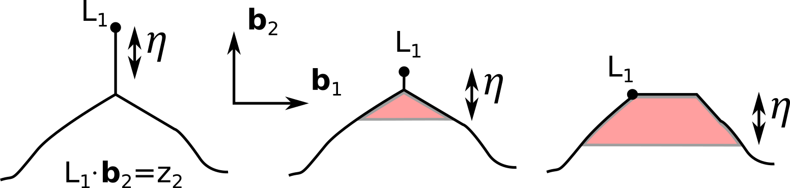
Figure 10: Neighbourhood of the north pole of three different curves. The position of the left extremity $L_{1}$ of the pole is marked by black dots. The volume $V_{1,\eta}$ at distance $\eta$ beneath the poles is the volume of the red area, which may vanish (left figure) if the ordinate $z_{1}=L_{1}\cdot{\bf b}_{2}$ of the north pole is at distance at least $\eta$ from the interior of the droplet associated with the curve.

$$z_{1}=\sup\{x\cdot{\bf b}_{2}:x\in\gamma\},\qquad z_{3}=\inf\{x\cdot{\bf b}_{2}:x\in\gamma\},$$

$$z_{2}=\sup\{x\cdot{\bf b}_{1}:x\in\gamma\},\qquad z_{4}=\inf\{x\cdot{\bf b}_{1}:x\in\gamma\}.$$ (4.23)

For $\eta>0$ and $1\leq k\leq 4$, define then the volume $V_{k,\eta}$ beneath pole $k$ as follows (recall that $\Gamma$ is the droplet with boundary $\gamma$):

$$V_{k,\eta}(\gamma)=\begin{cases}\big{|}\big{\{}x\in\Gamma:|z_{k}(\gamma)-x\cdot{\bf b}_{2}|\leq\eta\big{\}}\big{|}\quad\text{if }k\in\{1,3\},\\ \big{|}\big{\{}x\in\Gamma:|z_{k}(\gamma)-x\cdot{\bf b}_{1}|\leq\eta\big{\}}\big{|}\quad\text{if }k\in\{2,4\},\end{cases}\qquad\gamma\in\mathcal{E}.$$ (4.24)

Compared to the slope, the volume $V_{k,\eta}$ is more robust to changes in the position of the pole: it is not hard to check that $V_{k,\eta}$ is continuous on $\mathcal{E}$ in Hausdorff distance $d_{\mathcal{H}}$ (see (2.9)) for $1\leq k\leq 4$.
We claim that the reservoir-like behaviour of the poles implies that only trajectories satisfying a certain volume condition beneath the poles will be relevant for the large deviations. Indeed, in Lemma B.16, we establish that, for each $q,n\in\mathbb{N}^{*}$, there is $\eta(q,n)>0$ such that:

$$\sup_{\eta\leq\eta(q,n)}\limsup_{N\rightarrow\infty}\frac{1}{N}\log\mathbb{P}^{N}_{\beta,H} \bigg{(}\gamma^{N}_{\cdot}\in E([0,T],\mathcal{E});$$

$$\qquad\frac{1}{T}\int_{0}^{T}{\bf 1}\Big{\{}\big{|}\eta^{-2}V_{k,\eta}(\gamma^{N}_{t})-(e^{\beta}-1)\big{|}>\frac{1}{n}\Big{\}}dt>\frac{1}{n}\bigg{)}\leq-q.$$ (4.25)

In words and informally, (4.25) states that it is very unlikely for trajectories to spend longer than $T/n$ without the pole dynamics fixing the volume of a sufficiently small portion beneath each pole.
Simply by inclusion between the sets in the above probability, $n\mapsto\eta(q,n)$ can be taken to be decreasing. Up to reducing $\eta(q,n)$, we may also assume:

$$\forall q\in\mathbb{N}^{*},\qquad\lim_{n\rightarrow\infty}\eta(q,n)=0.$$ (4.26)

Define then a set $D_{q,n}$ with the following soft control of the poles:

$$D_{q,n} :=E([0,T],\mathcal{E})\cap\bigcap_{k=1}^{4}\bigg{\{}\forall m\in\{1,...,n\},$$ (4.27)

$$\qquad\frac{1}{T}\int_{0}^{T}{\bf 1}\Big{\{}\Big{|}\eta(q,m)^{-2}V_{k,\eta(q,m)}(\gamma_{t})-(e^{\beta}-1)\Big{|}>\frac{1}{m}\Big{\}}dt\leq\frac{1}{m}\bigg{\}}.$$

Since $V_{k,\eta}$ is continuous on $\mathcal{E}$ for the Hausdorff distance and the indicator function of an open set is lower semi-continuous, the set $D_{q,n}$ is closed in $E([0,T],\mathcal{E})$ for each $q,n\in\mathbb{N}^{*}$. Moreover, by (4.25):

$$\limsup_{N\rightarrow\infty}\frac{1}{N}\log\mathbb{P}^{N}_{\beta,H}\big{(}\gamma^{N}_{\cdot}\in D_{q,n}^{c}\cap E([0,T],\mathcal{E})\big{)}\leq-q.$$ (4.28)

By construction, for $q\in\mathbb{N}^{*}$, $D_{q,n^{\prime}}\subset D_{q,n}$ if $n\leq n^{\prime}$. As a result, as $n$ increases, the control on the behaviour of the poles of trajectories in $D_{q,n}$ gets finer. For $q\in\mathbb{N}^{*}$, define then $D_{q}$ as:

$$D_{q}:=\bigcap_{n\geq 1}D_{q,n}.$$ (4.29)

As stated in the next lemma, trajectories in each $D_{q}$, $q\in\mathbb{N}^{*}$ have almost always point-like poles (thus satisfy (4.18)), with kinks at each pole with slope $e^{-\beta}$.

Lemma 4.2.

Fix $q\in\mathbb{N}^{*}$, and let $(\gamma_{t})_{t\leq T}\in D_{q}$. Then, for each $k$ with $1\leq k\leq 4$:

$$\text{for a.e. }t\in[0,T],\qquad\liminf_{\eta\rightarrow 0}\big{|}\eta^{-2}V_{k,\eta}(\gamma_{t})-(e^{\beta}-1)\big{|}=0.$$ (4.30)

This in particular implies that $(\gamma_{t})_{t\leq T}$ has almost always point-like poles, thus, for future reference, that $\gamma_{t}$ is almost always a Jordan curve.

Before proving the lemma, let us establish the general upper bound (4.22). For $\zeta>0$, $n,q\in\mathbb{N}^{*}$ and $\beta>1$, write:

$$\limsup_{N\rightarrow\infty}\frac{1}{N}\log\mathbb{P}^{N}_{\beta}\Big{(} \gamma^{N}_{\cdot}\in B_{d_{E}}(\bar{\gamma}_{\cdot},\zeta)\cap E([0,T],\mathcal{E})\Big{)}$$

$$\qquad\leq\max\Big{\{}\limsup_{N\rightarrow\infty}\frac{1}{N}\log\mathbb{P}^{N}_{\beta}\Big{(}\gamma^{N}_{\cdot}\in B_{d_{E}}(\bar{\gamma}_{\cdot},\zeta)\cap D_{q,n}\Big{)},-q\Big{\}}.$$ (4.31)

By assumption, $\bar{\gamma}_{\cdot}$ does not have point-like poles. It thus does not belong to $D_{q}=\cap_{n}D_{q,n}$ by Lemma 4.2. Since $D_{q,n}\subset D_{q,n^{\prime}}$ for $n\geq n^{\prime}$, $\bar{\gamma}_{\cdot}$ does not belong to any $D_{q,n}$ for $n$ larger than some $n_{q}\in\mathbb{N}^{*}$. By construction, each $D_{q,n}$ is a closed set. There is thus $\zeta_{q}>0$ such that:

$$\forall\zeta\in(0,\zeta_{q}),\forall n\geq n_{q}\qquad B_{d_{E}}\big{(}\bar{\gamma}_{\cdot},\zeta\big{)}\cap D_{q,n}=\emptyset.$$ (4.32)

Injecting this in (4.31) proves the general upper bound (4.22):

$$\forall q\in\mathbb{N}^{*},\forall\zeta\in(0,\zeta_{q}),\qquad\limsup_{N\rightarrow\infty}\frac{1}{N}\log\mathbb{P}^{N}_{\beta}\Big{(} \gamma^{N}_{\cdot}\in B_{d_{E}}(\bar{\gamma}_{\cdot},\zeta)\cap E([0,T],\mathcal{E})\Big{)}\leq-q.$$ (4.33)

Remark 4.3 (Upper bound in Theorem 2.17).

To obtain (4.21)-(4.22), it is nowhere necessary that the trajectory $\bar{\gamma}_{\cdot}$ take values in $\mathcal{E}$ (i.e. be close to $\gamma^{\text{ref}}$ in volume at each time, see Definition 2.7). The only ingredient used is the fact that $\bar{\gamma}_{\cdot}$ is a trajectory of "nice" curves, i.e. curves satisfying Property 2.6. In this case, (4.21)-(4.22) correspond to the general upper bound in Theorem 2.17.  $\blacksquare$

We conclude the section with the proof of Lemma 4.2.

Proof of Lemma 4.2.

We consider the north pole $k=1$, the others are similar. Due to Property 2.1 in the definition of $\mathcal{E}$, a curve $\tilde{\gamma}\in\mathcal{E}$ does not have point-like north pole if and only if there is $c>0$ (the width of the north pole) such that, for any $\eta>0$ smaller than some $\eta_{0}(\tilde{\gamma})$:

$$V_{1,\eta}(\tilde{\gamma})\geq\eta c.$$ (4.34)

In particular, $\tilde{\gamma}$ has point-like north pole as soon as:

$$\liminf_{\eta\rightarrow 0}\eta^{-1}V_{1,\eta}(\tilde{\gamma})=0.$$ (4.35)

Fix a trajectory $(\gamma_{t})_{t\leq T}\in D_{q}$ and let $\varepsilon>0$. For each integer $n\geq 1/\varepsilon$, one has by definition of $D_{q}$:

$$\frac{1}{T}\int_{0}^{T}{\bf 1}\Big{\{}\big{|}\eta(q,n)^{-2}V_{1,\eta(q,n)}(\gamma_{t})-(e^{\beta}-1)\big{|}>\varepsilon\Big{\}}dt\leq\frac{1}{n}.$$ (4.36)

Since $\eta(q,n)$ vanishes when $n$ is large by definition (see (4.26)), this implies:

$$\liminf_{\eta\rightarrow 0}\int_{0}^{T}{\bf 1}\big{\{}\big{|}\eta^{-2}V_{1,\eta}(\gamma_{t})-(e^{\beta}-1)\big{|}>\varepsilon\big{\}}dt=0.$$ (4.37)

Using Fatou inequality, we find:

$$\int_{0}^{T} \liminf_{\eta\rightarrow 0}{\bf 1}\big{\{}\big{|}\eta^{-2}V_{1,\eta}(\gamma_{t})-(e^{\beta}-1)\big{|}>\varepsilon\big{\}}dt=0$$

$$\hskip 85.35826pt\quad\Rightarrow\quad\liminf_{\eta\rightarrow 0}{\bf 1}\big{\{}\big{|}\eta^{-2}V_{1,\eta}(\gamma_{t})-(e^{\beta}-1)\big{|}>\varepsilon\big{\}}=0\quad\text{for a.e }t\in[0,T]$$

$$\hskip 85.35826pt\quad\Rightarrow\quad\liminf_{\eta\rightarrow 0}\big{|}\eta^{-2}V_{1,\eta}(\gamma_{t})-(e^{\beta}-1)\big{|}\leq\varepsilon\quad\text{for a.e }t\in[0,T].$$ (4.38)

Since $\varepsilon$ is arbitrary, $\gamma_{\cdot}$ has almost always point-like north pole recalling (4.35). Moreover, the last equation, also valid for pole $k\neq 1$, implies that there are $d_{1},d_{2}>0$ such that, for almost every $t\in[0,T]$:

$$\exists\eta_{0}(t)>0,\forall 1\leq k\leq 4,\forall\eta\in(0,\eta_{0}(t)],\qquad\eta^{2}d_{1}\leq V_{k,\eta}(\gamma_{t})\leq\eta^{2}d_{2}.$$ (4.39)

For each such time $t$, the poles are point-like by (4.34), and at vanishing distance to the interior of the droplet: $\gamma_{t}$ is thus a Jordan curve. ∎

4.2 Upper bound on closed sets

Equipped with the bound (4.21), let us prove a large deviation bound for compact and closed sets in $E([0,T],\mathcal{E})$. The arguments are classical, and reproduced here for completeness.

Upper bound for compact sets. Let first $\mathcal{K}\subset E([0,T],\mathcal{E})$ be a compact set. Let $\eta>0$. By (4.21), for each $\bar{\gamma}_{\cdot}\in E([0,T],\mathcal{E})$, there is $\zeta(\bar{\gamma}_{\cdot})>0$ such that:

$$\limsup_{N\rightarrow\infty}\frac{1}{N}\log\mathbb{P}^{N}_{\beta}\Big{(}\gamma^{N}_{\cdot}\in B_{d_{E}}\big{(}\bar{\gamma}_{\cdot},\zeta(\bar{\gamma}_{\cdot})\big{)}\cap E([0,T],\mathcal{E})\Big{)}\leq-I_{\beta}(\bar{\gamma}_{\cdot}|\gamma^{\text{ref}})+\eta.$$ (4.40)

Cover the compact set $\mathcal{K}$ by $k_{\eta}\in\mathbb{N}^{*}$ balls $B_{d_{E}}\big{(}\bar{\gamma}^{i}_{\cdot},\zeta^{i}(\bar{\gamma}_{\cdot})\big{)}$, to find:

$$\limsup_{N\rightarrow\infty}\frac{1}{N}\log\mathbb{P}^{N}_{\beta}\Big{(}\gamma^{N}_{\cdot}\in\mathcal{K}\Big{)} \leq\max_{1\leq i\leq k_{\eta}}\big{(}-I_{\beta}(\bar{\gamma}^{i}_{\cdot}|\gamma^{\text{ref}})\big{)}+\eta$$

$$\leq-\inf_{\mathcal{K}}I_{\beta}(\cdot|\gamma^{\text{ref}})+\eta.$$ (4.41)

This proves the upper bound for compact sets.

Upper bound for closed sets. The upper bound for closed sets follow from the exponential tightness of $\big{(}\mathbb{P}^{N}_{\beta}(\cdot,E([0,T],\mathcal{E})\big{)}_{N}$ in $\mathcal{M}_{1}(E([0,T],\mathcal{E}))$, see Lemma 1.2.18 in [DZ10]. Establishing exponential tightness is quite technical, so we postpone it to Appendix B.3 and conclude here the upper bound of Theorem 2.15.

5 Lower bound large deviations and hydrodynamic limits

In this section, we prove the lower bound in Theorem 2.15. The method is classical (see [KL99]). It consists in using Jensen inequality and an expression of the Radon-Nikodym derivative $D^{N}_{\beta,H}:=d\mathbb{P}^{N}_{\beta,H}/d\mathbb{P}^{N}_{\beta}$ for a bias $H\in\mathcal{C}$, in Section 5.1, to turn the proof of the lower bound into a proof of the hydrodynamic limit for the tilted probability $\mathbb{P}^{N}_{\beta,H}$. The subtlety is that the contour dynamics is only well-controlled inside the effective state space $\mathcal{E}$. As basic ingredient to prove hydrodynamics, we thus need to know that trajectories under tilted dynamics typically remain in the effective state space $\mathcal{E}$ for short time. This is done in Section 5.2.1. We then prove hydrodynamics in short time (Section 5.2.2).
In case the limiting trajectory $\gamma^{H}_{\cdot}$ under $\mathbb{P}^{N}_{\beta,H}$, assumed to be unique, stays in the interior of the effective state space $\mathcal{E}$ longer than the short time of Section 5.2.2, we then prove, in Section 5.2.3, that hydrodynamics can be extended to later times.

5.1 A first lower-bound

Let $\beta>1$. Recall that, for a time $T>0$, $\mathcal{A}_{\beta,T}$ is the set of trajectories in $E_{pp}([0,T],\mathcal{E})$ assumed to be the unique solutions, for a bias $H\in\mathcal{C}$, of the weak formulation (2.41) of anisotropic motion by curvature with drift $H$. If $\mathcal{A}_{\beta,T}$ is empty, the lower bound in Theorem 2.15 is trivial. We work under the assumption:

$$\forall T>0,\qquad\mathcal{A}_{\beta,T}\neq\emptyset.$$ (5.1)

Recall also the definition of the set $\tilde{Z}(\beta,H,\delta,\varepsilon)$ for $H\in\mathcal{C}$ and $\varepsilon,\delta>0$ from Proposition 3.2. In this section, we prove the following.

Proposition 5.1.

Let $\beta>1$, $T>0$ and let $\gamma^{H}_{\cdot}\in\mathcal{A}_{\beta,T}$ be the trajectory associated with a bias $H\in\mathcal{C}$. Assume that $\gamma^{H}_{\cdot}$ is in the interior of $E([0,T],\mathcal{E})$:

$$\exists\zeta_{0}>0,\quad B_{d_{E}}(\gamma^{H}_{\cdot},\zeta)\subset E([0,T],\mathcal{E}).$$ (5.2)

$B_{d_{E}}(\gamma^{H}_{\cdot},\zeta)$ is the open ball of centre $\gamma^{H}_{\cdot}$ and radius $\zeta$ in $d_{E}$-distance. Then:

$$\liminf_{\zeta\rightarrow 0}\liminf_{N\rightarrow\infty}\frac{1}{N}\log\mathbb{P}^{N}_{\beta}\big{(}\gamma^{N}_{\cdot}\in B_{d_{E}}(\gamma^{H}_{\cdot},\zeta)\big{)}\geq-I_{\beta}(\gamma^{H}_{\cdot}|\gamma^{\text{ref}})$$ (5.3)

$$\hskip 56.9055pt+\inf_{\delta>0}\liminf_{\varepsilon\rightarrow 0}\liminf_{\zeta>0}\liminf_{N\rightarrow\infty}\frac{1}{N}\log\mathbb{P}^{N}_{\beta,H}\Big{(}\gamma^{N}_{\cdot}\in B_{d_{E}}(\gamma^{H}_{\cdot},\zeta)\cap\tilde{Z}(\beta,H,\delta,\varepsilon)\Big{)}.$$

Proof.

Let $H\in\mathcal{C}$ be as in the proposition and $\zeta,\delta,\varepsilon>0$. Write for short:

$$X:=B_{d_{E}}(\gamma^{H}_{\cdot},\zeta)\cap\tilde{Z}(\beta,H,\delta,\varepsilon).$$ (5.4)

One can write:

$$\log\mathbb{P}^{N}_{\beta}\big{(}\gamma^{N}_{\cdot}\in B_{d_{E}}(\gamma^{H}_{\cdot},\zeta)\big{)} \geq\log\mathbb{P}^{N}_{\beta,H}\big{(}\gamma^{N}_{\cdot}\in X\big{)}$$

$$=\log\Bigg{(}\frac{\mathbb{E}^{N}_{\beta,H}\Big{[}\big{(}D^{N}_{\beta,H}\big{)}^{-1}{\bf 1}_{\gamma^{N}_{\cdot}\in X}\Big{]}}{\mathbb{P}^{N}_{\beta}\big{(}\gamma^{N}_{\cdot}\in X\big{)}}\Bigg{)}+\log\mathbb{P}^{N}_{\beta,H}\big{(}\gamma^{N}_{\cdot}\in X\big{)}.$$ (5.5)

Jensen inequality applied to the logarithm then yields, dividing by $N$:

$$\frac{1}{N}\log\mathbb{P}^{N}_{\beta}\big{(}\gamma^{N}_{\cdot}\in\mathcal{O}\big{)}\geq-\frac{\mathbb{E}^{N}_{\beta,H}\Big{[}N^{-1}\log D^{N}_{\beta,H}{\bf 1}_{\gamma^{N}\in X_{\cdot}}\Big{]}}{\mathbb{P}^{N}_{\beta,H}\big{(}\gamma^{N}_{\cdot}\in X\big{)}}+\frac{1}{N}\log\mathbb{P}^{N}_{\beta,H}\big{(}\gamma^{N}_{\cdot}\in X\big{)}.$$ (5.6)

Taking the limits and infima as in the statement of Proposition 5.1, the second term already has the desired form. Let us compute the expectation. Notice first that elements of $B_{d_{E}}(\gamma^{H}_{\cdot},\zeta)$ have well controlled-length. Indeed, $\gamma^{H}_{\cdot}\in E([0,T],\mathcal{E})$ means that its length is integrable, so that there is $c(H,T)>0$ with:

$$\int_{0}^{T}|\gamma^{H}_{t}|dt\leq c(H,T).$$ (5.7)

One easily checks that the length of a curve $\gamma\in\mathcal{E}$ in $1$-norm is given in terms of the distance between the poles:

$$|\gamma|=2\big{[}L_{1}(\gamma)-L_{3}(\gamma)\big{]}\cdot{\bf b}_{2}+2\big{[}L_{2}(\gamma)-L_{4}(\gamma)\big{]}\cdot{\bf b}_{1}.$$ (5.8)

As each functional in the right-hand side is $1$-Lipschitz in Hausdorff distance (see Lemma B.3), we find:

$$\forall\gamma_{\cdot}\in B_{d_{E}}(\gamma^{H}_{\cdot},\zeta),\qquad\int_{0}^{T}|\gamma_{t}|dt\leq 8\int_{0}^{T}d_{\mathcal{H}}(\gamma^{H}_{t},\gamma_{t})dt+c(H,T)\leq 8\zeta+c(H,T).$$ (5.9)

Recall now the formula (4.3) for $N^{-1}\log D^{N}_{\beta,H}$: for $\gamma^{N}_{\cdot}\in E([0,T],\mathcal{E})$,

$$N^{-1}\log D^{N}_{\beta,H}(\gamma^{N}_{\cdot})=-J_{H,\varepsilon}^{\beta}(\gamma^{N}_{\cdot})+\int_{0}^{T}\omega(H_{t},\delta,\varepsilon,\gamma^{N}_{t})dt.$$ (5.10)

There is moreover $C(H)>0$ such that, for each $A>0$, on the set $\tilde{Z}(\beta,H,\delta,\varepsilon)\cap E([0,T],\mathcal{E})\cap\{\int_{0}^{T}|\gamma^{N}_{t}|dt\leq AT\}$, the quantity $\omega$ satisfies:

$$\Big{|}\int_{0}^{T}\omega(H_{t},\delta,\varepsilon,\gamma^{N}_{t})dt\Big{|}\leq 2\delta+C(H)T\Big{(}\varepsilon+\frac{A+1}{N}\Big{)}.$$ (5.11)

In view of the bound (5.9) on the length and taking the $\liminf$ in $N$, the expectation in  (5.6) is thus bounded from below as follows:

$$\liminf_{N\rightarrow\infty}-\frac{\mathbb{E}^{N}_{\beta,H}\Big{[}N^{-1}\log D^{N}_{\beta,H}{\bf 1}_{\gamma^{N}_{\cdot}\in X}\Big{]}}{\mathbb{P}^{N}_{\beta,H}\big{(}\gamma^{N}_{\cdot}\in X\big{)}}\geq\liminf_{N\rightarrow\infty}\frac{\mathbb{E}^{N}_{\beta,H}\Big{[}\big{(}-J_{H,\varepsilon}^{\beta}\big{)}{\bf 1}_{\gamma^{N}_{\cdot}\in X}\Big{]}}{\mathbb{P}^{N}_{\beta,H}\big{(}\gamma^{N}_{\cdot}\in X\big{)}}-2\delta-C(H)\varepsilon T.$$ (5.12)

Since $\gamma^{H}_{\cdot}\in E_{pp}([0,T],\mathcal{E})$, it is a point of continuity of $J_{H,\varepsilon}^{\beta}$ by Proposition 4.1. There is consequently a real function $m_{\beta,\gamma^{H}_{\cdot},H,\varepsilon}(\cdot)\geq 0$ such that:

$$\sup_{\gamma_{\cdot}\in B_{d_{E}}(\gamma^{H}_{\cdot},\zeta)}\big{|}J_{H,\varepsilon}^{\beta}(\gamma_{\cdot})-J^{\beta}_{H,\varepsilon}(\gamma^{H}_{\cdot})\big{|}=m_{\beta,\gamma^{H}_{\cdot},H,\varepsilon}(\zeta),\qquad\limsup_{\zeta\rightarrow 0}m_{\beta,\gamma^{H}_{\cdot},H,\varepsilon}(\zeta)=0.$$ (5.13)

As $B_{d_{E}}(\gamma^{H}_{\cdot},\zeta)\subset X$, the left-hand side of (5.12) is therefore bounded for small $\zeta$ by:

$$\liminf_{\zeta\rightarrow 0}\liminf_{N\rightarrow\infty}-\frac{\mathbb{E}^{N}_{\beta,H}\Big{[}N^{-1}\log D^{N}_{\beta,H}{\bf 1}_{\gamma^{N}_{\cdot}\in X}\Big{]}}{\mathbb{P}^{N}_{\beta,H}\big{(}\gamma^{N}_{\cdot}\in X\big{)}}\geq-J_{H,\varepsilon}^{\beta}(\gamma^{H}_{\cdot})-2\delta-C(H)\varepsilon T.$$ (5.14)

By Proposition 4.1, $J_{H,\varepsilon}^{\beta}(\gamma^{H}_{\cdot})$ converges to $J_{H}^{\beta}(\gamma^{H}_{\cdot})$ when $\varepsilon$ vanishes. Taking the liminf in $\varepsilon$, then the infimum on $\delta$ in the last equation thus turns its right-hand side into:

$$\inf_{\delta>0}\liminf_{\varepsilon\rightarrow 0}\Big{\{}-J_{H,\varepsilon}^{\beta}(\gamma^{H}_{\cdot})-2\delta-C(H)\varepsilon T\Big{\}}=-J_{H}^{\beta}(\gamma^{H}_{\cdot}).$$ (5.15)

To establish the claim of Proposition 5.1, it only remains to prove that $J^{\beta}_{H}(\gamma^{H}_{\cdot})=I_{\beta}(\gamma^{H}_{\cdot}|\gamma^{\text{ref}})$. For $G\in\mathcal{C}$, recall the definition (2.47) of $J^{\beta}_{G}$:

$$J^{\beta}_{G}(\gamma^{H}_{\cdot})=\ell_{G}(\gamma^{H}_{\cdot})-\frac{1}{2}\int_{0}^{T}\int_{\gamma^{H}_{t}}G^{2}\big{(}t,\gamma^{H}_{t}(s))\mu(\theta(s)\big{)}dsdt,$$ (5.16)

where $\ell^{\beta}_{G}$ is the functional defined in (2.46). Above, recall that, for a point $\gamma^{H}_{t}(s)$, $\theta(s)$ is the angle of the tangent vector ${\bf T}(\theta(s))=\cos(\theta(s)){\bf b}_{1}+\sin(\theta(s)){\bf b}_{2}$ with the horizontal axis at $\gamma^{H}_{t}(s)$.
From the weak formulation (2.41) of anisotropic motion by curvature, one has, for each $G\in\mathcal{C}$:

$$\ell^{\beta}_{G}(\gamma^{H}_{\cdot})=\int_{0}^{T}\int_{\gamma^{H}_{t}}G(t,\gamma^{H}_{t}(s))H\big{(}t,\gamma^{H}_{t}(s)\big{)}\mu(\theta(s))dsdt.$$ (5.17)

As a result,

$$I_{\beta}( \gamma^{H}_{\cdot}|\gamma^{\text{ref}}):=\sup_{G\in C}J^{\beta}_{G}(\gamma^{H}_{\cdot})$$

$$\ =\frac{1}{2}\int_{0}^{T}\int_{\gamma^{H}_{t}}H^{2}\big{(}t,\gamma^{H}_{t}(s)\big{)}\mu(\theta(s))dsdt+\sup_{G\in\mathcal{C}}\bigg{\{}-\frac{1}{2}\int_{0}^{T}\int_{\gamma^{H}_{t}}\big{[}G-H\big{]}^{2}\big{(}t,\gamma^{H}_{t}(s)\big{)}\mu(\theta(s))dsdt\bigg{\}}$$

$$\ =\frac{1}{2}\int_{0}^{T}\int_{\gamma^{H}_{t}}H^{2}\big{(}t,\gamma^{H}_{t}(s)\big{)}\mu(\theta(s))dsdt=J^{\beta}_{H}(\gamma^{H}_{\cdot}).$$ (5.18)

This concludes the proof of Proposition 5.1. ∎

5.2 Hydrodynamic limits for the tilted processes

In view of Proposition 5.1, the lower bound of Theorem 2.15 holds provided the expression involving the probability in (5.3) vanishes. This is the content of the next proposition.

Proposition 5.2.

With the notations of Proposition 5.1,

$$\inf_{\delta>0}\liminf_{\varepsilon\rightarrow 0}\liminf_{\zeta>0}\liminf_{N\rightarrow\infty}\frac{1}{N}\log\mathbb{P}^{N}_{\beta,H}\Big{(}\gamma^{N}_{\cdot}\in B_{d_{E}}(\gamma^{H}_{\cdot},\zeta)\cap\tilde{Z}(\beta,H,\delta,\varepsilon)\Big{)}=0.$$ (5.19)

The proof of Proposition 5.2 takes up Sections 5.2.1 to 5.2.3. We proceed as follows. First, we get rid of the technical condition that trajectories belong to $\tilde{Z}(\beta,H,\delta,\varepsilon)$, in Lemma 5.3. We then prove that trajectories typically stay in $E([0,T],\mathcal{E})$ for sufficiently small time $T>0$, in Section 5.2.1, thereby proving the first item of Proposition 2.9. This result is used in Section 5.2.2 to establish short time hydrodynamics for the tilted processes, making use of a generalised large deviation upper bound. This proves Proposition 5.2 for short time. Finally, in Section 5.2.3, we extend the short time hydrodynamics to the whole time interval $[0,T]$, concluding the proof of Proposition 5.2.

Let us first deal with $\tilde{Z}(\beta,H,\delta,\varepsilon)$.

Lemma 5.3.

With the notations of Proposition 5.1,

$$\inf_{\delta>0}\liminf_{\varepsilon\rightarrow 0}\liminf_{\zeta>0} \liminf_{N\rightarrow\infty}\frac{1}{N}\log\mathbb{P}^{N}_{\beta,H}\Big{(}\gamma^{N}_{\cdot}\in B_{d_{E}}(\gamma^{H}_{\cdot},\zeta)\cap\tilde{Z}(\beta,H,\delta,\varepsilon)\Big{)}$$

$$\qquad=\liminf_{\zeta>0}\liminf_{N\rightarrow\infty}\frac{1}{N}\log\mathbb{P}^{N}_{\beta,H}\Big{(}\gamma^{N}_{\cdot}\in B_{d_{E}}(\gamma^{H}_{\cdot},\zeta)\Big{)}.$$ (5.20)

Proof.

Write first:

$$\mathbb{P}^{N}_{\beta,H}\Big{(}\gamma^{N}_{\cdot}\in B_{d_{E}}(\gamma^{H}_{\cdot},\zeta)\cap\tilde{Z}(\beta,H,\delta,\varepsilon)\Big{)}$$

$$\hskip 56.9055pt=\mathbb{P}^{N}_{\beta,H}\Big{(}\gamma^{N}_{\cdot}\in B_{d_{E}}(\gamma^{H}_{\cdot},\zeta)\Big{)}-\mathbb{E}^{N}_{\beta}\Big{[}D^{N}_{\beta,H}{\bf 1}_{\gamma^{N}_{\cdot}\in B_{d_{E}}(\gamma^{H}_{\cdot},\zeta)\cap(\tilde{Z}(\beta,H,\delta,\varepsilon))^{c}}\Big{]}$$ (5.21)

Corollary 3.9 bounds the Radon-Nikodym derivative for trajectories in $E([0,T],\mathcal{E})$ as follows. There is $C(H)>0$ such that:

$$\forall\gamma^{N}_{\cdot}\in E([0,T],\mathcal{E}),\qquad D^{N}_{\beta,H}(\gamma^{N}_{\cdot})\leq\exp\bigg{[}C(H)N+C(H)\int_{0}^{T}|\gamma^{N}_{t}|dt\bigg{]}.$$ (5.22)

Since $B_{d_{E}}(\gamma^{H}_{\cdot},\zeta)\subset E([0,T],\mathcal{E})$ for small enough $\zeta$ by Assumption (5.2), the above bound is valid for microscopic trajectories in $B_{d_{E}}(\gamma^{H}_{\cdot},\zeta)$.
Let $\zeta>0$. For trajectories in $B_{d_{E}}(\gamma^{H}_{\cdot},\zeta)$, the time integral of the length is bounded by $c(H,T)+8\zeta$, see (5.9). As a result, for $\delta,\varepsilon>0$:

$$\Big{|}\mathbb{P}^{N}_{\beta,H}\Big{(}\gamma^{N}_{\cdot}\in B_{d_{E}}(\gamma^{H}_{\cdot},\zeta)\cap\tilde{Z}(\beta,H,\delta,\varepsilon)\Big{)}-\mathbb{P}^{N}_{\beta,H}\Big{(}\gamma^{N}_{\cdot}\in B_{d_{E}}(\gamma^{H}_{\cdot},\zeta)\Big{)}\Big{|}$$

$$\hskip 56.9055pt\leq e^{C(H)N+C(H)N(c(H,T)+8\zeta)}\mathbb{P}^{N}_{\beta}\Big{(}\gamma^{N}_{\cdot}\in B_{d_{E}}(\gamma^{H}_{\cdot},\zeta)\cap\big{(}\tilde{Z}(\beta,H,\delta,\varepsilon)\big{)}^{c}\Big{)}.$$ (5.23)

Moreover, by Proposition 3.2, for each $A>0$:

$$\limsup_{\varepsilon\rightarrow 0}\limsup_{N\rightarrow\infty}\frac{1}{N}\log\mathbb{P}^{N}_{\beta}\Big{(}\gamma^{N}_{\cdot}\in E([0,T],\mathcal{E})\cap\Big{\{}\int_{0}^{T}|\gamma_{t}|dt\leq AT\Big{\}}\cap\big{(}\tilde{Z}(\beta,H,\delta,\varepsilon)\big{)}^{c}\Big{)}=-\infty.$$ (5.24)

Since Assumption (5.2) and the bound (5.9) on the length imply $B_{d_{E}}(\gamma^{H}_{\cdot},\zeta)\subset E([0,T],\mathcal{E})\cap\big{\{}\int_{0}^{T}|\gamma_{t}|dt\leq AT\big{\}}$ for $AT\geq c(H,T)+8\zeta$, the above bound applies to estimate the right-hand side of (5.23). Taking the logarithm, dividing by $N$ and taking the liminf in $N$, then in $\zeta$, then in $\varepsilon$ in (5.23) yields the claim of the lemma. ∎

5.2.1 The droplet moves on a diffusive scale

In this section, we prove that trajectories typically stay in the effective state space $\mathcal{E}$ on a diffusive short time scale, corresponding to item $2$ of Proposition 2.9. Recall the convention that, for two interfaces $\gamma,\tilde{\gamma}\in\Omega$ with associated droplets $\Gamma,\tilde{\Gamma}$:

$$d_{L^{1}}(\gamma,\tilde{\gamma}):=d_{L^{1}}(\Gamma,\tilde{\Gamma}),\quad\text{with}\quad d_{L^{1}}(\Gamma,\tilde{\Gamma})=\int_{\mathbb{R}^{2}}|{\bf 1}_{\Gamma}-{\bf 1}_{\tilde{\Gamma}}|dudv.$$ (5.25)

Lemma 5.4 (Short-time stability of $\mathcal{E}$).

Let $\beta>1,H\in\mathcal{C}$. For each $\varepsilon>0$, there is a time $t(\varepsilon)=t(\beta,H,\varepsilon,|\gamma^{\text{ref}}|)>0$ such that:

$$\lim_{N\rightarrow\infty}\mathbb{P}^{N}_{\beta,H}\Big{(}\sup_{t\leq t(\varepsilon)}d_{L^{1}}\big{(}\gamma^{N}_{t},\gamma^{\text{ref}}\big{)}\leq\varepsilon\Big{)}=1.$$ (5.26)

In particular, let $\tilde{r}>0$ be a parameter such that (recall Definition 2.7 of $\mathcal{E}$):

$$B_{d_{L^{1}}}\big{(}\gamma^{\text{ref}},2\tilde{r}^{2}\big{)}\subset\mathcal{E}\quad\big{(}=B_{L^{1}}\big{(}\gamma^{\text{ref}},r_{0}^{2}\big{)}\big{)}.$$ (5.27)

Then, for each $\kappa$ larger than some $\kappa(\gamma^{\text{ref}})>0$, there is a time $t_{0}:=t_{0}(\beta,H,\tilde{r},\kappa)>0$ such that:

$$\lim_{N\rightarrow\infty}\inf_{\begin{subarray}{c}\gamma^{N}\in\Omega^{N}_{\text{mic}}:|\gamma^{N}|\leq\kappa\\ d_{L^{1}}(\gamma^{\text{ref}},\gamma^{N})\leq\tilde{r}\end{subarray}}\mathbb{P}^{\gamma^{N}}_{\beta,H}\Big{(}\gamma^{N}_{\cdot}\in E\big{(}[0,t_{0}],\mathcal{E}\big{)}\Big{)}=1.$$ (5.28)

Proof.

To prove (5.26), we use estimates that depend only on a bound on the length of the initial condition, and on its belonging to the interior of $\mathcal{E}$. Equation (5.28) will in particular directly follow from these estimates, so we only show (5.26).
Fix $H\in\mathcal{C}$. The proof of (5.26) is similar to the proof of the same statement in [Cap+11] for the stochastic Ising model. In both cases, the idea is that changing the volume of the droplet requires adding or deleting a number of blocks of order $N^{2}$, which takes time. The additional difficulty in the present case comes from the pole dynamics: droplets can grow.
To deal with growth, we prove in Lemma 6.1 that, under $\mathbb{P}^{N}_{\beta,H}$, the length of a curve typically stays of order $N$ on the diffusive scale. More precisely, for each $\beta>1$ and $T>0$, there is $C(\beta,H,T)>0$ such that, for each $A>0$:

$$\limsup_{N\rightarrow\infty}\frac{1}{N}\log\mathbb{P}^{N}_{\beta,H}\Big{(}\gamma^{N}_{\cdot}\in E([0,T],\mathcal{E})\cap\Big{\{} \sup_{t\leq T}|\gamma^{N}_{t}|\geq A\Big{\}}\Big{)}$$

$$\qquad\leq-C(\beta,H,T)A+|\gamma^{\text{ref}}|\beta.$$ (5.29)

Take then $\kappa_{H}>0$ such that the right-hand side of (5.29) is strictly negative.
For trajectories with length bounded as above, we will be able to use the following result. Recall the convention (5.25) that the volume distance between two curves is the volume distance between their respective droplets.

Lemma 5.5.

Let $\varepsilon,\kappa>0$. There are functions $J_{1},J_{2}\in C^{2}_{c}(\mathbb{R}^{2},[0,1])$, depending only on $\varepsilon,\kappa$ and $\gamma^{\text{ref}}$, such that for any curve $\gamma\in\mathcal{E}$ with length $|\gamma|\leq\kappa$ and $d_{L^{1}}(\gamma,\gamma^{\text{ref}})\geq\varepsilon$, the following holds:

$$\max_{i\in\{1,2\}}\big{|}\big{<}\Gamma,J_{i}\big{>}-\big{<}\Gamma^{\text{ref}},J_{i}\big{>}\big{|}\geq\varepsilon/4,\quad\text{where}\quad\big{<}\Gamma,J_{i}\big{>}:=\int_{\Gamma}J_{i}(u,v)dudv.$$ (5.30)

Let us momentarily admit Lemma 5.5, established at the end of the section, and prove (5.26). Let $\varepsilon>0$, and $t^{\,\text{st}}_{\varepsilon}$ denote the first time $t\geq 0$ such that:

$$d_{L^{1}}\big{(}\gamma^{N}_{t},\gamma^{\text{ref}}\big{)}\geq\varepsilon.$$ (5.31)

Without loss of generality, we may assume $\varepsilon\in(0,\tilde{r}]$ with $\tilde{r}$ as in (5.27). Introduce the dynamics $\mathbb{P}^{N,st}_{\beta,H}$, corresponding to $\mathbb{P}^{N}_{\beta,H}$, but stopped at time $t^{\,\text{st}}_{\varepsilon}$. Then, for each $t\geq 0$:

$$\mathbb{P}^{N}_{\beta,H}\big{(}t^{\,\text{st}}_{\varepsilon}\leq t\big{)} =\mathbb{P}^{N,st}_{\beta,H}\big{(}t^{\,\text{st}}_{\varepsilon}\leq t\big{)}$$

$$=\mathbb{P}^{N,st}_{\beta,H}\Big{(}\gamma^{N}_{\cdot}\in E([0,t],\mathcal{E})\cap\big{\{}t^{\,\text{st}}_{\varepsilon}\leq t\big{\}}\Big{)}$$

$$=\mathbb{P}^{N,st}_{\beta,H}\Big{(}\gamma^{N}_{\cdot}\in E([0,t],\mathcal{E})\cap\Big{\{}\sup_{t^{\prime}\leq t}|\gamma^{N}_{t^{\prime}}|\leq\kappa_{H}\Big{\}}\cap\big{\{}t^{\,\text{st}}_{\varepsilon}\leq t\big{\}}\Big{)}+o_{N}(1).$$ (5.32)

The second equality comes from $\varepsilon\leq\tilde{r}$, which ensures that trajectories always stay in $\mathcal{E}$ under $\mathbb{P}^{N,st}_{\beta,H}$. The last equality follows from (5.29), below which $\kappa_{H}$ is defined. By Lemma 5.5, there are functions $J_{1},J_{2}\in C^{2}_{c}(\mathbb{R}^{2},[0,1])$ depending only on $\Gamma^{\text{ref}},\varepsilon,\kappa_{H}$, such that:

$$\mathbb{P}^{N,st}_{\beta,H}\Big{(}\gamma^{N}_{\cdot}\in E([0,t],\mathcal{E})\cap\Big{\{}\sup_{t^{\prime}\leq t}|\gamma^{N}_{t^{\prime}}|\leq\kappa_{H}\Big{\}}\cap\big{\{}t^{\,\text{st}}_{\varepsilon}\leq t\big{\}}\Big{)}$$ (5.33)

$$\qquad\leq\mathbb{P}^{N,st}_{\beta,H}\Big{(}\gamma^{N}_{\cdot}\in E([0,t],\mathcal{E})\cap\Big{\{}\sup_{t^{\prime}\leq t}|\gamma^{N}_{t^{\prime}}|\leq\kappa_{H}\Big{\}}\cap\Big{\{}\max_{i\in\{1,2\}}\sup_{t^{\prime}\leq t}\big{|}\big{<}\Gamma^{N}_{t^{\prime}},J_{i}\big{>}-\big{<}\Gamma^{\text{ref}},J_{i}\big{>}\big{|}\geq\varepsilon/4\Big{\}}\Big{)}$$

$$\qquad\leq\mathbb{P}^{N}_{\beta,H}\Big{(}\gamma^{N}_{\cdot}\in E([0,t],\mathcal{E})\cap\Big{\{}\sup_{t^{\prime}\leq t}|\gamma^{N}_{t^{\prime}}|\leq\kappa_{H}\Big{\}}\cap\Big{\{}\max_{i\in\{1,2\}}\sup_{t^{\prime}\leq t}\big{|}\big{<}\Gamma^{N}_{t^{\prime}},J_{i}\big{>}-\big{<}\Gamma^{\text{ref}},J_{i}\big{>}\big{|}\geq\varepsilon/4\Big{\}}\Big{)}.$$

To estimate the last probability, let us write, for each $i\in\{1,2\}$ and $t^{\prime}\leq t$:

$$\big{<}\Gamma^{N}_{t^{\prime}},J_{i}\big{>}-\big{<}\Gamma^{\text{ref}},J_{i}\big{>}=\frac{1}{N}\log A^{J_{i}}_{t^{\prime}}+\frac{1}{N}\log D^{N}_{\beta,J}\big{(}(\gamma^{N}_{u})_{u\leq t^{\prime}}\big{)},$$ (5.34)

with $D^{N}_{\beta,J}$ the Radon-Nikodym derivative defined in (4.1) (here we implicitly set $J(t,\cdot)=J(\cdot)$ for each $t\geq 0$), and:

$$\forall i\in\{1,2\},\forall t^{\prime}\leq t,\qquad\log A^{J_{i}}_{t^{\prime}}:=\int_{0}^{t}N^{2}e^{-N\big{<}\Gamma^{N}_{u},J_{i}\big{>}}\mathcal{L}_{\beta}e^{N\big{<}\Gamma^{N}_{u},J_{i}\big{>}}du.$$ (5.35)

The bounds of Corollary 3.9 apply to $A^{J_{i}}_{\cdot}$ for trajectories with values in $\mathcal{E}$: for some $C(J_{i})>0$ (depending on $\varepsilon$ through $J_{i}$),

$$\forall\gamma^{N}_{\cdot}\in E([0,T],\mathcal{E}),\qquad\sup_{t^{\prime}\leq t}\frac{1}{N}\big{|}\log A^{J_{i}}_{t^{\prime}}(\gamma^{N}_{\cdot})\big{|}\leq C(H)C(J_{i})\int_{0}^{t}|\gamma^{N}_{t}|dt.$$ (5.36)

As a result, for each $i\in\{1,2\}$, one has (recall that $D^{N}_{\beta,{J_{i}}}\geq 0$):

$$\mathbb{P}^{N}_{\beta,H}\Big{(}\gamma^{N}_{\cdot}\in E([0,t],\mathcal{E})\cap\Big{\{}\sup_{t^{\prime}\leq t}|\gamma^{N}_{t^{\prime}}|\leq\kappa_{H}\Big{\}}\cap\Big{\{}\sup_{t^{\prime}\leq t}\big{|}\big{<}\Gamma^{N}_{t^{\prime}},J_{i}\big{>}-\big{<}\Gamma^{\text{ref}},J_{i}\big{>}\big{|}\geq\varepsilon/4\Big{\}}\Big{)}$$

$$\quad=\mathbb{P}^{N}_{\beta,H}\Big{(}\gamma^{N}_{\cdot}\in E([0,t],\mathcal{E})\cap\Big{\{}\sup_{t^{\prime}\leq t}|\gamma^{N}_{t^{\prime}}|\leq\kappa_{H}\Big{\}}\cap\Big{\{}\sup_{t^{\prime}\leq t}D^{N}_{\beta,J_{i}}\geq e^{N\varepsilon/4-C(H)C(J_{i})\kappa_{H}t}\Big{\}}\Big{)}.$$ (5.37)

Since $D^{N}_{\beta,J_{i}}$ is a mean-1 martingale, Doob’s maximal inequality yields:

$$\mathbb{P}^{N}_{\beta,H}\Big{(}\sup_{t^{\prime}\leq t}D^{N}_{\beta,J_{i}}\geq e^{N\varepsilon/4-C(H)C(J_{i})\kappa_{H}t}\Big{)} \leq e^{-N\varepsilon/4+C(H)C(J_{i})\kappa_{H}t}\mathbb{E}^{N}_{\beta,H}\big{[}D^{N}_{\beta,J_{i}}((\gamma^{N}_{t^{\prime}})_{t^{\prime}\leq t})\big{]}$$

$$=e^{-N\varepsilon/4+C(H)C(J_{i})\kappa_{H}t}.$$ (5.38)

From (5.32) and the last inequality, it follows that $\mathbb{P}^{N}_{\beta,H}(t^{\,\text{st}}_{\varepsilon}\leq t)$ vanishes with $N$ as soon as $t\leq\varepsilon/(4\kappa_{H}C(H)\max\{C(J_{1}),C(J_{2})\})$, which concludes the proof of (5.26) admitting Lemma 5.5.

Proof of Lemma 5.5. Let us now prove Lemma 5.5. Let $\varepsilon,\kappa>0$ and $\gamma\in\mathcal{E}$ be such that:

$$|\gamma|\leq\kappa,\quad d_{L^{1}}(\gamma,\gamma^{\text{ref}})\geq\varepsilon.$$ (5.39)

Let $\Gamma$ be the associated droplet. Then one has:

$$\text{either}\quad|\Gamma\setminus\Gamma^{\text{ref}}|\geq\varepsilon/2,\qquad\text{or}\quad|\Gamma^{\text{ref}}\setminus\Gamma|\geq\varepsilon/2.$$ (5.40)

Let $J_{1}\in C^{2}_{c}(\mathbb{R}^{2},[0,1])$ be a smooth approximation of ${\bf 1}_{\Gamma^{\text{ref}}}$, and $J_{2}\in C^{2}_{c}(\mathbb{R}^{2},[0,1])$ a smooth approximation of ${\bf 1}_{(\Gamma^{\text{ref}})^{c}}$ cut off at distance $\kappa$ from $\Gamma^{\text{ref}}$ in $1$-norm. One can choose $J_{1},J_{2}$ as a function of $\Gamma^{\text{ref}}$ and $\varepsilon$ in such a way that:

$$|\Gamma\setminus\Gamma^{\text{ref}}|\geq\varepsilon/2\quad\Rightarrow\quad\big{<}\Gamma,J_{2}\big{>}-\big{<}\Gamma^{\text{ref}},J_{2}\big{>}\geq\varepsilon/4,$$

$$|\Gamma^{\text{ref}}\setminus\Gamma|\geq\varepsilon/2\quad\Rightarrow\quad\big{<}\Gamma^{\text{ref}},J_{1}\big{>}-\big{<}\Gamma,J_{1}\big{>}\geq\varepsilon/4.$$ (5.41)

This concludes the proof of Lemma 5.5, thus of Lemma 5.4. ∎

5.2.2 Short-time hydrodynamics

Proposition 5.6.

[Short time hydrodynamics] Let $\beta>1$. Let $T>0$ and $H\in\mathcal{C}$ be such that the weak formulation (2.41) with drift $H$ has a unique solution $\gamma^{H}_{\cdot}\in E([0,T],\mathcal{E})$ starting from the initial condition $\gamma^{\text{ref}}$ of Definition 2.5. For $\kappa>0$ large enough depending on $\gamma^{\text{ref}}$, let $(\mu^{N})_{N}$ be a sequence of probability measures on $\big{(}\mathcal{E},d_{L^{1}}\big{)}$, converging weakly to $\delta_{\gamma^{\text{ref}}}$ and such that:

$$\limsup_{N\rightarrow\infty}\mu^{N}\big{(}|\gamma^{N}|\geq\kappa\big{)}=0.$$ (5.42)

Let $t_{0}=t_{0}(\beta,H,\tilde{r},\kappa)\in(0,T]$ be the time of Lemma 5.4, with $\tilde{r}$ a parameter satisfying:

$$B_{d_{L^{1}}}\big{(}\gamma^{\text{ref}},2\tilde{r}^{2}\big{)}\subset\mathcal{E}.$$ (5.43)

Then:

$$\forall\zeta>0,\qquad\limsup_{N\rightarrow\infty}\mathbb{P}^{\mu^{N}}_{\beta,H}\bigg{(}\gamma^{N}_{\cdot}\notin B_{d_{E}}\big{(}(\gamma^{H}_{t})_{t\leq t_{0}},\zeta\big{)}\bigg{)}=0.$$ (5.44)

Proposition 5.6 is implied by the following lemma, in which hydrodynamics for $(\mathbb{P}^{N}_{\beta,H})_{N}$ are established in short time thanks to Lemma 5.4 and the uniqueness assumption on solutions of (2.41). The proof of Lemma 5.7 in particular contains the proof of Proposition 2.11.

Lemma 5.7.

Let $\beta>1$, $H\in\mathcal{C}$, $\kappa>0$, $t_{0}$ and the sequence $(\mu^{N})_{N}$ be as in Proposition 5.6. Then $(\mathbb{P}^{N}_{\beta,H})_{N}$ converges to $\delta_{(\gamma^{H}_{t})_{t\leq t_{0}}}$ in the weak topology of probability measures on $E([0,t_{0}],\Omega)$, with $\Omega$ the general state space given in Definition 2.2. In particular (5.44) holds.

Proof.

The complementary of the ball $B_{d_{E}}((\gamma^{H}_{t})_{t\leq t_{0}},\zeta)$ is closed in $E([0,t_{0}],\Omega)$ for each $\zeta>0$. Equation (5.44) is therefore a direct consequence of the weak convergence result, which we now prove.
The hypothesis (5.42) on the initial law $\mu^{N}$ ensures, by Lemma 5.4, that:

$$\lim_{N\rightarrow\infty}\mathbb{P}^{\mu^{N}}_{\beta,H}\Big{(}\gamma^{N}_{\cdot}\in E([0,t_{0}],\mathcal{E})\Big{)}=1.$$ (5.45)

Under this condition, in Appendix B.3 (see Corollary B.13), the sequence $\{\mathbb{P}^{\mu^{N}}_{\beta,H}:N\in\mathbb{N}^{*}\}$ is proven to be relatively compact in $E([0,t_{0}],\Omega)$, with limit points supported in trajectories in $E([0,t_{0}],\mathcal{E})$ that are continuous in $d_{L^{1}}$ distance. Let $\mathbb{P}^{*}_{\beta,H}$ be one of its limit points. In view of (4.28) and Lemma 5.4, $\mathbb{P}^{*}_{\beta,H}$ is supported on trajectories with almost always point-like poles (they are in the set $D_{q}$ defined in (4.29) for each $q\in\mathbb{N}^{*}$), starting from a curve $\gamma^{0}$ with $d_{L^{1}}(\gamma^{0},\gamma^{\text{ref}})=0$.

To prove that $\mathbb{P}^{*}_{\beta,H}=\delta_{(\gamma^{H}_{t})_{t\leq t_{0}}}$, let us prove that $\mathbb{P}^{*}_{\beta,H}$ concentrates on trajectories that satisfy the weak formulation (2.41) of anisotropic motion by curvature on $[0,t_{0}]$. This is sufficient to conclude the proof of Lemma 5.7, because we have assumed that $(\gamma^{H}_{t})_{t\leq t_{0}}$ is the unique solution of (2.41) on $[0,t_{0}]$.
To prove this concentration property, the standard idea is (see e.g. Chapter 4 in [KL99]) to start from the following semi-martingale representation: if $t\geq 0$, $G\in\mathcal{C}$ and $(\Gamma^{N}_{t})_{t\geq 0}$ is as usual the trajectory of droplets associated with microscopic curves $(\gamma^{N}_{t})_{t\geq 0}$,

$$\big{<}\Gamma^{N}_{t},G_{t}\big{>}=\big{<}\Gamma^{N}_{0},G_{0}\big{>}+\int_{0}^{t}\big{<}\Gamma_{u},\partial_{u}G_{u}\big{>}du+\int_{0}^{t}N^{2}\mathcal{L}_{\beta,H}\big{<}\Gamma^{N}_{u},G_{u}\big{>}du+M^{N,G}_{t},$$ (5.46)

where $(M^{N,G}_{t})_{t}$ is a martingale. By assumption, $\gamma^{N}_{0}$ converges in $d_{L^{1}}$-distance to the initial condition $\gamma^{\text{ref}}$ of the trajectory $\gamma^{H}_{\cdot}$. The point is thus to compute the action of the generator $\mathcal{L}_{\beta,H}$ above, defined with the jump rates $c^{H}$ of (2.31), and prove that it approximates the right-hand side of (2.41). This is done in exactly the same way as the computation of the Radon-Nikodym derivative in Section 3.2, so we conclude the proof here. ∎

The proof of Proposition 5.6 is thus complete.

5.2.3 Extension to later times

In this section, the notations are those of Proposition 5.1. We extend the result of Proposition 5.6 to the whole time interval $[0,T]$ on which $\gamma^{H}_{\cdot}$ is assumed to take values in the interior of $\mathcal{E}$ in the sense of (5.2). This concludes the proof of Proposition 5.2, thereby concluding the proof of lower bound large deviations as stated in Proposition 5.1.

Proposition 5.8.

Let $\beta>1$, $T>0$, and let $H\in\mathcal{C}$ be such that there is a unique solution $(\gamma^{H}_{t})_{t\leq T}\in E([0,T],\mathcal{E})$ of the weak formulation (2.41) of anisotropic motion by curvature with drift $H$. Assume that $\gamma^{H}_{\cdot}$ stays in the interior of $\mathcal{E}$ until time $T$ in the following sense:

$$\exists r_{H}>0,\forall t\in[0,T],\qquad B_{d_{L^{1}}}\big{(}\gamma^{H}_{t},2r_{H}^{2}\big{)}\subset\mathcal{E}.$$ (5.47)

Then:

$$\forall\zeta>0,\qquad\lim_{N\rightarrow\infty}\mathbb{P}^{N}_{\beta,H}\Big{(}\gamma^{N}_{\cdot}\in E([0,T],\mathcal{E})\cap B_{d_{E}}(\gamma^{H}_{\cdot},\zeta)\Big{)}=1.$$ (5.48)

Remark 5.9 (Lower bound in Theorem 2.17).

Let us stress that Proposition 5.8 is still a short-time result in the sense that we only consider trajectories that stay in the small neighbourhood $\mathcal{E}$ of the reference curve $\gamma^{\text{ref}}$.
One should therefore understand Proposition 5.8 as stating that, if $\gamma^{H}_{\cdot}$ stays inside $\mathcal{E}$ up to a time $T$ larger than the small time $t_{0}$ of Lemma 5.4 (which was determined without using any property of $\gamma^{H}_{\cdot}$), then hydrodynamics are valid up to time $T$.

However, the proof of Proposition 5.8 does not rely on trajectories remaining close to $\gamma^{\text{ref}}$ (i.e. taking values in $\mathcal{E}$), but only on being "nice", in the sense that they satisfy Property 2.6 like $\gamma^{\text{ref}}$ at each time (this is the point of Assumption (5.47)). In particular, the lower bound of Theorem 2.17, which is a genuine long-time result, follows from the proof of Proposition 5.8 with only notational changes.  $\blacksquare$

Combining Proposition 5.8 and Lemma 5.3 yields Proposition 5.2, since the assumption (5.2) that $\gamma^{H}_{\cdot}$ is in the interior of $E([0,T],\mathcal{E})$ and the continuity of $t\mapsto\gamma^{H}_{t}$ in $d_{L^{1}}$ distance (obtained in the proof of Lemma 5.7) implies (5.47). Let us now prove Proposition 5.8.

Proof.

The claim of Proposition 5.8 is proven in Proposition 5.6 up to the time $t_{0}(\beta,H,\tilde{r},|\gamma^{\text{ref}}|)\in(0,T]$ of Lemma 5.6. The point here is to show that the result holds up to time $T$.
To do so, the idea is to iterate the results of Section 5.2.2 on small time intervals. These intervals are built thanks to the condition (5.47) and a bound on the length as follows. By Lemma 6.1, there is $\kappa_{H}>0$ such that, for each $t\leq T$:

$$\limsup_{N\rightarrow\infty}\mathbb{P}^{N}_{\beta,H}\Big{(}\gamma^{N}_{\cdot}\in E([0,t],\mathcal{E})\cap\Big{\{}\sup_{t^{\prime}\leq t}|\gamma^{N}_{t^{\prime}}|\geq\kappa_{H}\Big{\}}\Big{)}=0.$$ (5.49)

Recalling the definition of $r_{H}$ from (5.47), one can then consider intervals of length:

$$t_{H}:=\min\big{\{}t_{0}(\beta,H,r_{H},\kappa_{H}),t_{0}(\beta,H,\tilde{r},|\gamma^{\text{ref}}|)\big{\}}>0,$$ (5.50)

and apply Proposition 5.6 on each of these intervals as we shall see. Let $n:=\lfloor T/t_{H}\rfloor+1$, and let us prove by recursion on $1\leq i\leq n$ that hydrodynamics hold up to time $it_{H}$, i.e.:

$$\forall\zeta>0,\qquad\lim_{N\rightarrow\infty}\mathbb{P}^{N}_{\beta,H}\Big{(}\gamma^{N}_{\cdot}\in E([0,it_{H}],\mathcal{E})\cap B_{d_{E}}\big{(}(\gamma^{H}_{t})_{t\leq it_{H}},\zeta\big{)}\Big{)}=1.$$ (5.51)

On $[0,t_{H}]$, Proposition 5.6 yields:

$$\forall\zeta>0,\qquad\lim_{N\rightarrow\infty}\mathbb{P}^{N}_{\beta,H}\Big{(}\gamma^{N}_{\cdot}\in E([0,t_{H}],\mathcal{E})\cap B_{d_{E}}\big{(}(\gamma^{H}_{t})_{t\leq t_{H}},\zeta\big{)}\Big{)}=1,$$ (5.52)

which is the $i=1$ claim. Assume the claim holds up to $i-1<n$. To prove that it holds at rank $i$, it is enough to prove:

$$\forall\zeta>0,\qquad\lim_{N\rightarrow\infty}\mathbb{P}^{N}_{\beta,H}\Big{(}E([(i-1)t_{H},it_{H}],\mathcal{E})\cap B_{d_{E}}\big{(}(\gamma^{H}_{t})_{(i-1)t_{H}\leq t\leq it_{H}},\zeta\big{)}\Big{)}=1.$$ (5.53)

To prove the last equation, we would like to use the Markov property, then apply Proposition 5.6. To do so, we need to check that the law $\mathbb{P}^{N}_{\beta,H}(\gamma^{N}_{(i-1)t_{H}}\in\cdot)$ of $\gamma^{N}_{(i-1)t_{H}}$ concentrates on curves with bounded lengths in the sense of (5.42), and converges to $\delta_{\gamma^{H}_{(i-1)t_{H}}}$ for the weak topology associated with $d_{L^{1}}$. We prove it as follows.
Equation (5.49) applied to $t=(i-1)t_{H}$ and the recursion hypothesis bounds the length of supported trajectories:

$$\lim_{N\rightarrow\infty}\mathbb{P}^{N}_{\beta,H}\Big{(}\sup_{t\leq(i-1)t_{H}}|\gamma^{N}_{t}|\geq\kappa_{H}\Big{)}=0.$$ (5.54)

Moreover, as $\gamma^{H}_{\cdot}$ is continuous in $d_{L^{1}}$-distance, the mapping $\gamma_{\cdot}\in E([0,T],\mathcal{E})\mapsto d_{L^{1}}(\gamma_{t},\gamma^{H}_{t})$ is continuous for the distance $d_{E}$ for each time $t\in[0,T]$. The hydrodynamic limit up to time $(i-1)t_{H}$, given by the recursion hypothesis, then yields the desired convergence (in fact also in probability rather than only weakly):

$$\forall\eta>0,\qquad\lim_{N\rightarrow\infty}\mathbb{P}^{N}_{\beta,H}\Big{(}\gamma^{N}_{(i-1)t_{H}}\in B_{d_{L^{1}}}\big{(}\gamma^{H}_{(i-1)t_{H}},\eta\big{)}\Big{)}=1.$$ (5.55)

For short, write $\mu^{N}_{i-1}$ for the law of $\gamma^{N}_{(i-1)t_{H}}$. As a result of the last two estimates and the Markov property, (5.53) holds as soon as:

$$\forall\zeta>0,\qquad \lim_{N\rightarrow\infty}\mathbb{P}^{\mu^{N}_{i-1}}_{\beta,H}\Big{(}\gamma^{N}_{\cdot}\in E([0,it_{H}],\mathcal{E})\cap B_{d_{E}}\big{(}(\gamma^{H}_{t})_{(i-1)t_{H}\leq t\leq it_{H}},\zeta\big{)}\Big{)}=1.$$ (5.56)

By Assumption (5.47), $\gamma^{H}_{(i-1)t_{H}}$ satisfies the property (5.43) demanded of $\gamma^{\text{ref}}$ in Proposition 5.6, with $\tilde{r}$ there replaced by $r_{H}$. We also just checked that the initial condition $\mu^{N}_{i-1}$ satisfies the same properties as the initial condition of Proposition 5.6, with $\gamma^{\text{ref}}$ replaced by $\gamma^{H}_{(i-1)t_{H}}$. Proposition 5.6 thus applies to prove (5.56). This completes the induction step and the proof of Proposition 5.8. ∎

6 Behaviour of the poles and ${\bf 1}_{p_{k}=2}$ terms

In this section, we focus on the specificity of the contour dynamics: the behaviour of the poles. This section is central to the proof of large deviations. There are two main results. The first is the control of the length of a curve, which is the first item of Proposition 2.9. The second is the proof of Proposition 2.10, which states that the regrowth, $e^{-2\beta}$ term in the generator (2.22) can be seen as the action of a moving reservoir of particles, fixing the density of vertical edges in its vicinity in terms of $\beta$, i.e. the tangent vector at each pole. The proof of this statement is carried out in Subsection 6.3. It makes crucial use of the irreducibility of the dynamics around the poles, which is the single added feature in the contour dynamics compared to the zero temperature stochastic Ising model.
Subsection 6.2 presents a useful bijection argument, used to both estimate the pole size and establish local equilibrium at the poles. These two statements were used in Sections 3-4. A bias $H\in\mathcal{C}$ are fixed throughout the section.

6.1 Control of the length of a curve

This section is devoted to the proof of the first item of Proposition 2.9, i.e. the control of the supremum of the length of a trajectory. This estimate is central to the proof of large deviations: it enables one to prove, in Corollary 6.2, that if an event has probability decaying super-exponentially fast under $\mathbb{P}^{N}_{\beta}$, then this remains true under the tilted dynamics $\mathbb{P}^{N}_{\beta,H}$, $H\in\mathcal{C}$.

Lemma 6.1.

Let $\beta>\log 2$ and $T>0$. There is then $C(\beta)>0$ such that:

$$\forall A>0,\qquad\limsup_{N\rightarrow\infty}\frac{1}{N}\log\mathbb{P}^{N}_{\beta}\Big{(}\sup_{t\leq T}|\gamma^{N}_{t}|\geq A\Big{)}\leq-C(\beta)A+|\gamma^{\text{ref}}|\beta.$$ (6.1)

Moreover, take a bias $H\in\mathcal{C}$. There are constants $C(\beta,H,T),C(H)>0$ with $t\mapsto C(\beta,H,t)$ increasing, such that:

$$\forall T,A>0,\qquad \limsup_{N\rightarrow\infty}\frac{1}{N}\log\mathbb{P}^{N}_{\beta,H}\Big{(}E([0,T],\mathcal{E})\cap\Big{\{}\sup_{t\leq T}|\gamma^{N}_{t}|\geq A\Big{\}}\Big{)}$$

$$\hskip 142.26378pt\leq-C(\beta,H,T)A+|\gamma^{\text{ref}}|\beta+C(H).$$ (6.2)

Proof.

The proof relies on the structure of the invariant measure. We start with the $H\equiv 0$ case.
First, as $\beta>\log 2$, the partition function $\mathcal{Z}^{N}_{\beta}$ normalising $\nu^{N}_{\beta}$ (see (2.16)) is bounded. One has, for some $c^{0}>0$ such that $|\gamma^{N,0}|\leq|\gamma^{\text{ref}}|+c^{0}/N$ for each $N$:

$$\mathbb{P}^{N}_{\beta}\Big{(}\sup_{t\leq T}|\gamma^{N}_{t}|\geq A\Big{)} \leq\nu^{N}_{\beta}(\gamma^{\text{ref},N})^{-1}\mathbb{P}^{\nu^{N}_{\beta}}_{\beta}\Big{(}\sup_{t\leq T}|\gamma^{N}_{t}|\geq A\Big{)}$$

$$\leq\mathcal{Z}^{N}_{\beta}e^{\beta(N|\gamma^{\text{ref}}|+c^{0})}\mathbb{P}^{\nu^{N}_{\beta}}_{\beta}\Big{(}\sup_{t\leq T}|\gamma^{N}_{t}|\geq A\Big{)}.$$ (6.3)

Let $b>0$ to be fixed later, and split the time interval $[0,T]$ into $N^{b}$ slices of length $TN^{-b}$ to obtain, using the invariance of $\nu^{N}_{\beta}$:

$$\mathbb{P}^{N}_{\beta}\Big{(}\sup_{t\leq T}|\gamma^{N}_{t}|\geq A\Big{)}\leq\mathcal{Z}^{N}_{\beta}N^{b}e^{\beta N(|\gamma^{\text{ref}}|+c^{0})}\mathbb{P}^{\nu^{N}_{\beta}}_{\beta}\Big{(}\sup_{t\leq N^{-b}T}|\gamma^{N}_{t}|\geq A\Big{)}.$$ (6.4)

To estimate the last probability, let us decompose $|\gamma^{N}_{\cdot}|$: for each $t\geq 0$,

$$|\gamma^{N}_{t}|=|\gamma^{N}_{0}|+\frac{1}{N}\log V_{t}+\frac{1}{N}\log D_{t},$$ (6.5)

where $D_{\cdot}$ is a mean-$1$ exponential martingale, and $V_{\cdot}$ is the finite variation process given by:

$$\forall t\geq 0,\qquad\frac{1}{N}\log V_{t} :=\frac{1}{N}\int_{0}^{t}e^{-N|\gamma^{N}_{s}|}N^{2}\mathcal{L}_{\beta}e^{N|\gamma^{N}_{s}|}dt$$ (6.6)

$$=N\int_{0}^{t}\sum_{k=1}^{4}\big{[}e^{-2\beta}(p_{k}(\gamma^{N}_{u})-1)\big{(}e^{2}-1\big{)}+{\bf 1}_{p_{k}(\gamma^{N}_{u})=2}{\bf 1}_{(\gamma^{N})^{-,k}\in\Omega_{\text{mic}}^{N}}\big{(}e^{-2}-1)\big{]}du.$$

To estimate the probability in (6.4), it is enough to separately estimate the probability that $|\gamma^{N}_{0}|\geq A$, and the probability of the suprema of each of the other two terms in (6.5). Let us start with $|\gamma^{N}_{0}|$. Since the number of curves in $\Omega^{N}_{\text{mic}}$ with $n\in\mathbb{N}^{*}$ edges is bounded by $cn^{4}2^{n}$ for some $c>0$, the following equilibrium estimate holds:

$$\nu^{N}_{\beta}\Big{(}|\gamma^{N}|\geq A\Big{)}\leq\frac{1}{\mathcal{Z}^{N}_{\beta}}\sum_{n\geq AN}cn^{4}2^{n}e^{-\beta n}=O\big{(}e^{-AN\beta^{\prime}}\big{)},\quad 0<\beta^{\prime}<\beta-\log 2.$$ (6.7)

Consider now the finite variation term (6.6). Bounding each $p_{k}$ by $CN$ for some $C>0$ and using Chebychev inequality to obtain the second line below, we find:

$$\mathbb{P}^{\nu^{N}_{\beta}}_{\beta}\Big{(}\sup_{t\leq N^{-b}T}\frac{1}{N}\log V_{t}\geq A\Big{)} \leq\mathbb{P}^{\nu^{N}_{\beta}}_{\beta}\Big{(}\frac{N^{2}\big{(}e^{2}-1\big{)}}{2}\int_{0}^{TN^{-b}}\sum_{k=1}^{4}p_{k}(\gamma^{N}_{s})ds\geq\frac{ANe^{2\beta}}{4}\Big{)}$$

$$\leq\exp\Big{[}-\frac{ANe^{2\beta}}{4(e^{2}-1)}\Big{]}e^{CTN^{3-b}/2}$$

$$\leq e^{CT/2}e^{-ANe^{2\beta}(e^{2}-1)^{-1}/4}\quad\text{ for }b\geq 3.$$ (6.8)

Consider finally the martingale term $\frac{1}{N}\log D_{t}$in (6.5). As $D_{t}$ is a mean-1 positive martingale, Doob’s martingale inequality gives:

$$\mathbb{P}^{\nu^{N}_{\beta}}_{\beta}\Big{(}\sup_{t\leq N^{-b}T}\frac{1}{N}\log D_{t}\geq A\Big{)}\leq e^{-AN}\mathbb{E}^{\nu^{N}_{\beta}}_{\beta}\big{[}D_{N^{-b}T}\big{]}=e^{-AN}.$$ (6.9)

Putting (6.7)-(6.8)-(6.9) together yields the claim of Lemma 6.1 when $H\equiv 0$.

Take now $H\in\mathcal{C}$, and let us prove (6.2). Recall from Corollary 3.9 that there is $C(H)>0$ such that the Radon-Nikodym derivative $D^{N}_{\beta,H}=d\mathbb{P}^{N}_{\beta,H}/d\mathbb{P}^{N}_{\beta}$ satisfies, for each $T>0$:

$$\forall\gamma^{N}_{\cdot}\in E([0,T],\mathcal{E}),\qquad\log D^{N}_{\beta,H}(\gamma^{N}_{\cdot})\leq\exp\Big{[}C(H)N+C(H)N\int_{0}^{T}|\gamma^{N}_{t}|dt\Big{]}.$$ (6.10)

We will prove the following: until time $t_{*}=t_{*}(\beta,H):=C(\beta)/(2C(H))$, for each $A>0,\kappa>0$ and each initial condition $\gamma^{N}_{0}\in\mathcal{E}$ with length bounded by $\kappa$:

$$\limsup_{N\rightarrow\infty}\frac{1}{N}\log\mathbb{P}^{N}_{\beta,H}\Big{(}E([0,t_{*}],\mathcal{E})\cap\Big{\{}\sup_{t\leq t_{*}}|\gamma_{t}^{N}|\geq A\Big{\}}\Big{)}\leq-C(\beta)A/2+\kappa\beta+C(H).$$ (6.11)

Assuming (6.11) holds, let us conclude the proof of Lemma 6.1. Let $n_{*}\in\mathbb{N}$ be such that $(n_{*}-1)t_{*}\leq T\leq n_{*}t_{*}$, and define a sequence $(b_{i})_{i\in\mathbb{N}}$ through:

$$b_{0}=0,\qquad\frac{C(\beta)b_{i+1}}{2}=C(\beta)+b_{i}(\beta+\log 2),\quad i\in\mathbb{N}.$$ (6.12)

Write then:

$$\mathbb{P}^{N}_{\beta,H}\Big{(}E([0,T],\mathcal{E})\cap\Big{\{}\sup_{t\leq T}|\gamma^{N}_{t}|\geq b_{n_{*}}A\Big{\}}\Big{)}$$

$$\quad\leq\mathbb{P}^{N}_{\beta,H}\Big{(}\gamma_{(n_{*}-1)t_{*}}\in\mathcal{E},\sup_{t\leq n_{*}t_{*}}|\gamma^{N}_{t}|\geq b_{n_{*}}A,\sup_{t\leq(n_{*}-1)t_{*}}|\gamma^{N}_{t}|<b_{n_{*}-1}A\Big{)}$$

$$\hskip 56.9055pt+\mathbb{P}^{N}_{\beta,H}\Big{(}E([0,(n_{*}-1)t_{*}],\mathcal{E})\cap\Big{\{}\sup_{t\leq(n_{*}-1)t_{*}}|\gamma^{N}_{t}|\geq b_{n_{*}-1}A\Big{\}}\Big{)}$$

$$\quad\leq\sum_{i=2}^{n_{*}}\mathbb{P}^{N}_{\beta,H}\Big{(}\gamma^{N}_{(i-1)t_{*}}\in\mathcal{E},\sup_{t\leq it_{*}}|\gamma^{N}_{t}|\geq b_{i}A,\sup_{t\leq(i-1)t_{*}}|\gamma^{N}_{t}|<b_{i-1}A\Big{)}$$

$$\hskip 56.9055pt+\mathbb{P}^{N}_{\beta,H}\Big{(}E([0,t_{*}],\mathcal{E})\cap\Big{\{}\sup_{t\leq t_{*}}|\gamma^{N}_{t}|\geq b_{1}A\Big{\}}\Big{)}.$$ (6.13)

The last probability is estimated by (6.11). On the other hand, apply Markov inequality to each term of the sum to find, for $2\leq i\leq n_{*}$:

$$\mathbb{P}^{N}_{\beta,H}\Big{(}\gamma^{N}_{(i-1)t_{*}}\in\mathcal{E},\sup_{t\leq it_{*}}|\gamma^{N}_{t}|\geq b_{i}A,\sup_{t\leq(i-1)t_{*}}|\gamma^{N}_{t}|<b_{i-1}A\Big{)}$$

$$\qquad\leq\sup_{\begin{subarray}{c}\gamma^{N}\in\Omega^{N}_{\text{mic}}\cap\mathcal{E}\\ |\gamma^{N}|<b_{i-1}A\end{subarray}}\mathbb{P}^{\gamma^{N}}_{\beta,H}\Big{(}\sup_{t\leq t_{*}}|\gamma^{N}_{t}|\geq b_{i}A\Big{)}.$$ (6.14)

Using (6.11) and the fact that there is $c>0$ such that the number of curves with $\ell$ edges in $\Omega^{N}_{\text{mic}}$ is less than $c\ell^{4}2^{\ell}$, we find for $2\leq i\leq n_{*}$:

$$\limsup_{N\rightarrow\infty}\frac{1}{N}\log\mathbb{P}^{N}_{\beta,H}\Big{(}\sup_{t\leq it_{*}}|\gamma^{N}_{t}|\geq b_{i}A,\sup_{t\leq(i-1)t_{*}}|\gamma^{N}_{t}|<b_{i-1}A\Big{)}$$

$$\hskip 85.35826pt\leq-\frac{C(\beta)b_{i}A}{2}+b_{i-1}(\beta+\log 2)A+C(H)=-C(\beta)A+C(H).$$ (6.15)

This estimate and (6.11) corresponding to $i=1$ prove (6.2) assuming (6.11), with $C(\beta,H,T):=b_{n_{*}}^{-1}$.
Let us now prove the short time estimate (6.11). Starting again from (6.10), one has, for each $T>0$:

$$\mathbb{P}^{N}_{\beta,H}\Big{(}\Big{\{}\sup_{t\leq T}|\gamma^{N}_{t}|\geq A\Big{\}}\cap E([0,T],\mathcal{E})\Big{)} \leq e^{C(H)N}\mathbb{E}^{N}_{\beta}\Big{[}e^{C(H)NT\sup_{t\leq T}|\gamma^{N}_{t}|}{\bf 1}_{\sup_{t\leq T}|\gamma^{N}_{t}|\geq A}\Big{]}.$$ (6.16)

By (6.1), this expectation reads:

$$\mathbb{E}^{N}_{\beta}\Big{[}e^{C(H)NT\sup_{t\leq T}|\gamma^{N}_{t}|}{\bf 1}_{\sup_{t\leq T}|\gamma_{t}|\geq A}\Big{]} \leq\int_{A}^{\infty}e^{C(H)NT\lambda}\mathbb{P}^{N}_{\beta}\Big{(}\sup_{t\leq T}|\gamma^{N}_{t}|\geq\lambda\Big{)}d\lambda$$

$$\leq\int_{A}^{\infty}e^{C(H)NT\lambda-c(\beta)N\lambda+|\gamma^{\text{ref}}|\beta N}d\lambda.$$ (6.17)

Setting $t_{*}(\beta,H):=C(\beta)/(2C(H))$ concludes the proof of (6.11), thus of Lemma 6.1. ∎

The following corollary explains how to use Lemma 6.1 to argue that events with super-exponentially small probability under $\mathbb{P}^{N}_{\beta}$ also have super-exponentially small probability under the tilted dynamics $\mathbb{P}^{N}_{\beta,H}$ for $H\in\mathcal{C}$. Typical examples are the sets $(D_{n,q})_{q}$ for fixed $n$, see (4.27), and $Z=Z(\beta,H,\varepsilon,\delta)$ for $\varepsilon\leq\varepsilon_{0}(\delta)$ and $\delta>0$, see (4.12).

Corollary 6.2 (Sub-exponential estimates for tilted dynamics).

For a time $T>0$, let $(\chi_{A,T})_{A>0}\subset E([0,T],\Omega)$ be a family of sets such that, for some $C(\beta)>0$:

$$\forall T>0,\forall A>0,\qquad\limsup_{N\rightarrow\infty}\frac{1}{N}\log\mathbb{P}^{\nu^{N}_{\beta}}_{\beta}\Big{(}\chi_{A,T}^{c}\cap E([0,T],\mathcal{E})\Big{)}\leq-C(\beta)A.$$ (6.18)

Then, for each $H\in\mathcal{C}$ and each time $T>0$, there are constants $C(\beta,H,T),C(H)>0$ with $t\mapsto C(\beta,H,t)$ increasing (different from those of Lemma 6.1), such that:

$$\forall T,A>0,\quad\limsup_{N\rightarrow\infty}\frac{1}{N}\log\mathbb{P}^{N}_{\beta,H}\Big{(}\chi_{A,T}^{c}\cap E([0,T],\mathcal{E})\Big{)}\leq-C(\beta,H,T)A+C(H)+|\gamma^{\text{ref}}|\beta.$$ (6.19)

Proof.

Let $A^{\prime}>0$, and write first, using Corollary 3.9:

$$\mathbb{P}^{N}_{\beta,H}\Big{(}\chi_{A,T}^{c}\cap E([0,T],\mathcal{E})\Big{)} \leq\mathbb{E}^{N}_{\beta}\Big{[}{\bf 1}_{\chi_{A,T}^{c}\cap E([0,T],\mathcal{E})\cap\{\sup_{t\leq T}|\gamma^{N}_{t}|\leq A^{\prime}\}}D^{N}_{\beta,H}\Big{]}+\mathbb{P}^{N}_{\beta,H}\Big{(}\sup_{t\leq T}|\gamma^{N}_{t}|\geq A^{\prime}\Big{)}$$

$$\leq e^{C(H)N(1+A^{\prime}T)}\mathbb{P}^{N}_{\beta}\Big{(}\chi_{A,T}^{c}\cap E([0,T],\mathcal{E})\cap\big{\{}\sup_{t\leq T}|\gamma^{N}_{t}|<A^{\prime}\big{\}}\Big{)}$$

$$\quad+\mathbb{P}^{N}_{\beta,H}\Big{(}\sup_{t\leq T}|\gamma_{t}|\geq A^{\prime}\Big{)}.$$ (6.20)

The first probability is controlled by (6.18), the second by the tail estimates for the length obtained in Lemma 6.1, so we conclude the proof here. ∎

6.2 Size of the poles and local equilibrium

In this section, we prove Lemmas 3.4-3.5, i.e. we estimate the time integral of the number of blocks $p_{1}$ in the north pole $P_{1}$, and of the term:

$$W^{G}_{t}(\gamma^{N}):=\sum_{\begin{subarray}{c}x\in P_{1}(\gamma^{N})\\ x+{\bf e}^{\pm}_{x}\in P_{1}(\gamma^{N})\end{subarray}}\big{(}{\bf 1}_{p_{1}(\gamma^{N})=2,(\gamma^{N})^{-,1}\in\Omega^{N}_{\text{mic}}}-e^{-2\beta}\big{)}G(t,x),\qquad\gamma^{N}\in\Omega^{N}_{\text{mic}},t\geq 0.$$ (6.21)

for any test function $G\in\mathcal{C}$.
Notation: in the following, we write simply $P$ for the north pole, $p$ for its number of blocks. Moreover, as we only deal with microscopic curves, we remove the superscript $N$ on curves, simply writing $\gamma$ for $\gamma^{N}\in\Omega_{\text{mic}}^{N}$.

Lemma 6.3.

Let $T>0$. For each $N\in\mathbb{N}^{*}$ and each $0<a<N/2$,

$$\mathbb{E}^{\nu_{\beta}}_{\beta}\Big{[}\exp\Big{[}aN\int_{0}^{T}e^{-2\beta}(p(\gamma_{t})-1)dt\Big{]}\Big{]}\leq\exp\Big{[}NaT+\frac{2Na^{2}T}{N-2a}\Big{]},$$ (6.22)

so that for each $A>1$:

$$\limsup_{N\rightarrow\infty}\frac{1}{N}\log\mathbb{P}^{N}_{\beta}\left(\frac{1}{T}\int_{0}^{T}e^{-2\beta}(p(\gamma_{t})-1)dt\geq A\right)=-\infty.$$ (6.23)

Moreover, for each $\delta>0$ and $G\in\mathcal{C}$,

$$\limsup_{N\rightarrow\infty}\frac{1}{N}\log\mathbb{P}^{N}_{\beta}\biggr{(}\bigg{|}\frac{1}{T}\int_{0}^{T}W^{G}_{t}(\gamma_{t})dt\bigg{|}>\delta\bigg{)}=-\infty.$$ (6.24)

By Corollary 6.2, the limits (6.23)-(6.24) hold also under $\mathbb{P}^{N}_{\beta,H}$ with the additional condition that trajectories belong to $E([0,T],\mathcal{E})$.

The proof of Lemma 6.3 relies on a bijection argument, stated in the following lemma, for which more notations are required.
If $\gamma\in\Omega^{N}_{\text{mic}}$ (recall that we drop the $N$ superscript on microscopic curves), let $p^{\prime}(\gamma)$ denote the number of blocks with centre at height $z_{1}(\gamma)-\frac{3}{2N}$ in the associated droplet $\Gamma$ (see Figure 11):

$$p^{\prime}(\gamma):=\Big{|}\Big{\{}\text{blocks in }\Gamma\text{ with centre }i\text{ with }i\cdot{\bf b}_{2}=z_{1}(\gamma)-\frac{3}{2N}\Big{\}}\Big{|},$$ (6.25)

where $z_{1}$ is the largest ordinate of points in a curve:

$$\quad z_{1}(\gamma):=\sup\big{\{}x\cdot{\bf b}_{2}:x\in\gamma\big{\}}.$$ (6.26)

Write also $\nu$ for the measure $\nu^{N}_{\beta}$. The expectation under the static measure $\nu$ is denoted by $E_{\nu}$, $E_{\nu_{f}}$ is the expectation under $f\nu$ when $f$ is a density for $\nu$, and $\nu_{f}$ denotes the associated probability. Define the Dirichlet form $D_{N}$ of the contour dynamics:

$$D_{N}(g):=-E_{\nu}\Big{[}g\mathcal{L}_{\beta}g\Big{]}=\frac{1}{2}\sum_{\gamma,\tilde{\gamma}\in\Omega^{N}_{\text{mic}}}\nu(\gamma)c(\gamma,\tilde{\gamma})\big{[}g(\gamma)-g(\tilde{\gamma})\big{]}^{2},\qquad g:\Omega^{N}_{\text{mic}}\rightarrow\mathbb{R}.$$ (6.27)

Lemma 6.4.

Let $f$ be a density with respect to the contour measure $\nu$. Then, for any integer $A\geq 2$,

$$\Big{[}\nu_{f}\big{(}p=2,\gamma^{-,1}\in\Omega^{N}_{\text{mic}},p^{\prime}\geq A\big{)}^{1/2}-E_{\nu_{f}}\big{[}(p-1)e^{-2\beta}{\bf 1}_{p\geq A}\big{]}^{1/2}\Big{]}^{2}\leq 2D_{N}(f^{1/2}).$$ (6.28)

The indicator function ${\bf 1}\gamma^{-,1}\in\Omega^{N}_{\text{mic}}$ in the first probablity ensures that the deletion of a pole is a dynamically allowed move.
Equation (6.28) also holds with $p^{\prime}\leq A,p\leq A$ instead of $p^{\prime}\geq A,p\geq A$ respectively in the probability and in the expectation.

Proof.

We prove the result with $A=2$ (i.e. without constraint on $p^{\prime}$), the general case is similar. Fix a density $f$ for $\nu$, and define $U$ on $\Omega^{N}_{\text{mic}}$ as follows:

$$\forall\gamma\in\Omega^{N}_{\text{mic}},\qquad U(\gamma)=e^{-2\beta}(p(\gamma)-1).$$ (6.29)

Let us prove that $\nu_{f}(p=2,\gamma^{-,1}\in\Omega^{N}_{\text{mic}})$ and $E_{\nu_{f}}[U]$ are comparable, up to an error that can be expressed in terms of the Dirichlet form $D_{N}(f^{1/2})$.

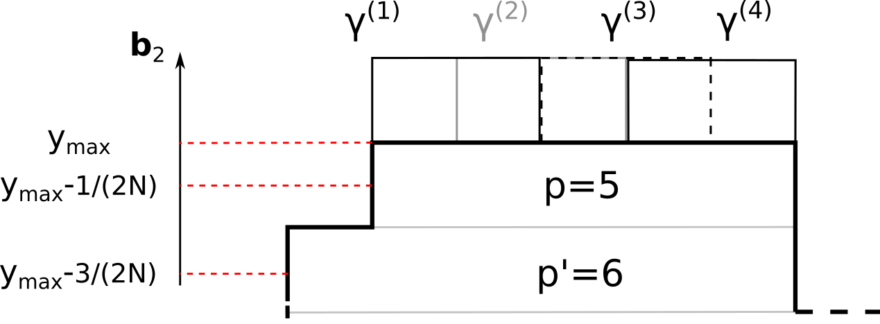
Figure 11: Neighbourhood of the north pole of a curve $\gamma\in\Omega^{N}_{\text{mic}}$ (thick line) and the $\gamma^{(n)}$, $n\leq p-1=4$. $\gamma^{(3)}$ is the curve $\gamma$ to which the two blocks delimited by dashed lines are added. Conversely, any of the $\gamma^{(n)}$, $n\leq 4$ is in $\{p=2,\gamma^{-,1}\in\Omega^{N}_{\text{mic}}\}$, and deleting the two blocks constituting their poles turns them into $\gamma$. The curve $\gamma$ has $p=5$ blocks in the pole, corresponding to blocks with centre at height $z_{1}-\frac{1}{2N}$, and $p^{\prime}=6$ blocks on the level below, i.e. with centre at height $z_{1}-\frac{3}{2N}$.

Each $\gamma\in\Omega^{N}_{\text{mic}}$ can be turned into any one of the curves $\gamma^{(1)},...,\gamma^{(p-1)}$ with two blocks added atop the north pole, where $\gamma^{(n)}$ is identical to $\gamma$ except that two blocks sitting on the edges $n,n+1$ are added, counting the edges from the left extremity of the pole (see Figure 11). Note that the $\gamma^{(n)}$ correspond to the $\gamma^{+,x}$ with $x,x+{\bf e}^{\pm}_{x}\in P$ defined in Definition 2.3.
Conversely, the north pole of each curve $\tilde{\gamma}\in\big{\{}p=2,\gamma^{-,1}\in\Omega^{N}_{\text{mic}}\big{\}}$ can be deleted, to obtain a curve $\gamma=(\tilde{\gamma})^{-,1}$ which is still in $\Omega^{N}_{\text{mic}}$, with the notations of Section 2. The curve $\gamma$ has length $|\gamma|=|\tilde{\gamma}|-2/N$. The same curve $\gamma$ can be obtained $p-1=p(\gamma)-1$ times by deleting a pole of size $2$, i.e. by performing the opposite move as those depicted in Figure 11. This means that $\tilde{\gamma}$ is either one of the curves $\gamma^{(n)}$ of Figure 11 for $1\leq n\leq p-1$. Thus:

$$\nu_{f}\big{(}p=2,\gamma^{1,-}\in\Omega^{N}_{\text{mic}}\big{)} =\sum_{\tilde{\gamma}\in\{p=2,\gamma^{-,1}\in\Omega^{N}_{\text{mic}}\}}\nu(\tilde{\gamma})f(\tilde{\gamma})$$

$$=\sum_{\tilde{\gamma}\in\{p=2,\gamma^{-,1}\in\Omega^{N}_{\text{mic}}\}}\sum_{\gamma\in\Omega^{N}_{\text{mic}}}{\bf 1}_{\{\exists n\leq p-1:\tilde{\gamma}=\gamma^{(n)}\}}\nu(\gamma)e^{-2\beta}f(\gamma^{(n)})$$

$$=\sum_{\gamma\in\Omega^{N}_{\text{mic}}}\nu(\gamma)e^{-2\beta}\sum_{n=1}^{p-1}f(\gamma^{(n)}).$$ (6.30)

Add and subtract the quantities needed to bound the second line by the Dirichlet form $D_{N}(f^{1/2})$:

$$\nu_{f}\big{(}p=2,\gamma^{-,1}\in\Omega^{N}_{\text{mic}}\big{)} =\sum_{\gamma\in\Omega^{N}_{\text{mic}}}\nu(\gamma)e^{-2\beta}\sum_{n=1}^{p-1}\big{[}f(\gamma^{(n)})+f(\gamma)-2f^{1/2}(\gamma)f^{1/2}(\gamma^{(n)})\big{]}$$

$$\hskip 28.45274pt-\sum_{\gamma\in\Omega^{N}_{\text{mic}}}\nu(\gamma)e^{-2\beta}\Big{[}(p-1)f(\gamma)-2\sum_{n=1}^{p-1}f^{1/2}(\gamma)f^{1/2}(\gamma^{(n)})\Big{]}.$$ (6.31)

To estimate the second line of (6.31), apply Cauchy-Schwarz inequality to the sum $\sum_{k=1}^{p-1}$ to obtain:

$$\nu_{f}\big{(}p=2,\gamma^{-,1}\in\Omega^{N}_{\text{mic}}\big{)} \leq 2D_{N}(f^{1/2})-E_{\nu_{f}}\big{[}e^{-2\beta}(p-1)\big{]}$$

$$\qquad+2\sum_{\gamma\in\Omega^{N}_{\text{mic}}}\nu(\gamma)e^{-2\beta}(p-1)^{1/2}f^{1/2}(\gamma)\Big{[}\sum_{n=1}^{p-1}f(\gamma^{(n)})\Big{]}^{1/2}.$$ (6.32)

Recall the definition of $U$ from (6.29) and again use Cauchy-Schwarz on the sum on $\gamma\in\Omega^{N}_{\text{mic}}$ to find:

$$\nu_{f}\big{(}p=2,\gamma^{-,1}\in\Omega^{N}_{\text{mic}}\big{)} \leq 2D_{N}(f^{1/2})-E_{\nu_{f}}[U]$$

$$\qquad+2\Big{[}\sum_{\gamma\in\Omega^{N}_{\text{mic}}}\nu(\gamma)e^{-2\beta}(p-1)f(\gamma)\Big{]}^{1/2}\Big{[}\sum_{\gamma\in\Omega^{N}_{\text{mic}}}\nu(\gamma)e^{-2\beta}\sum_{n=1}^{p-1}f(\gamma^{(n)})\Big{]}^{1/2}$$

$$=2D_{N}(f^{1/2})-E_{\nu_{f}}[U]+2E_{\nu_{f}}[U]^{1/2}\nu_{f}\big{(}p=2,\gamma^{-,1}\in\Omega^{N}_{\text{mic}}\big{)}^{1/2}.$$ (6.33)

Putting things together yields the claim of the lemma:

$$\Big{[}\nu_{f}\big{(}p=2,\gamma^{-,1}\in\Omega^{N}_{\text{mic}}\big{)}^{1/2}-E_{\nu_{f}}[U]^{1/2}\Big{]}^{2}\leq 2D_{N}(f^{1/2}).$$ (6.34)

∎

Proof of Lemma 6.3.

We now explain how to obtain Lemma 6.3 from Lemma 6.4. We need to do two things:

1. Bound from above the probabilities appearing in the claim by an expression involving the measure $\nu_{f}$ as in (6.28).

2. Prove that (6.24) holds for $W_{\cdot}^{G}$, with $G\in\mathcal{C}$. The first point only gives the result for ${\bf 1}_{p=2,\gamma^{-,1}\in\Omega^{N}_{\text{mic}}}-U$, which corresponds to $W^{1}_{\cdot}$;.

The first point relies on a classical Feynman-Kac estimate. Since a similar reasoning is used repeatedly in the article, we present it here once and for all. The second point, however, requires some care; in order to apply the bounds of Lemma 6.4 to integrals depending on a function $G\in\mathcal{C}$.

Let us explain the general idea for the first point using (6.23) as an example. We wish to estimate:

$$\mathbb{P}^{N}_{\beta}\left(\frac{1}{T}\int_{0}^{T}e^{-2\beta}(p(\gamma_{t})-1)dt\geq A\right).$$ (6.35)

We do so using Feynman-Kac formula. Let $a>0$, and apply the exponential Chebychev inequality to obtain

$$\frac{1}{N}\log\mathbb{P}^{N}_{\beta} \left(\frac{1}{T}\int_{0}^{T}e^{-2\beta}(p(\gamma_{t})-1)dt\geq A\right)$$ (6.36)

$$\leq-aAT+\frac{1}{N}\log\mathbb{E}^{N}_{\beta}\left[\exp\left[aN\int_{0}^{T}e^{-2\beta}(p(\gamma_{t})-1)dt\right]\right].$$

Consider the generator $N^{2}\mathcal{L}_{\beta}+aNU$, with $U$ defined in (6.29). This generator is self-adjoint for the contour measure $\nu_{\beta}$, and Feynman-Kac inequality plus a representation theorem for the largest eigenvalue of a symmetric operator (Lemma A.1.7.2 in [KL99]) yield that, with the equilibrium measure $\nu=\nu^{N}_{\beta}$ as an initial condition:

$$\mathbb{E}^{\nu}_{\beta}\biggr{[}\exp\left[aN\int_{0}^{T}U(\gamma_{t})dt\right]\biggr{]}\leq\exp\bigg{[}\int_{0}^{T}\sup_{f\geq 0:E_{\nu}[f]=1}\Big{\{}aNE_{\nu_{f}}[U]-N^{2}D_{N}(f^{1/2})\Big{\}}dt\bigg{]}.$$ (6.37)

In the present, $G\equiv 1$ case, the supremum in (6.37) does not depend on time.
One can bound $\mathbb{P}^{N}_{\beta}$, where the initial condition is the deterministic curve $\gamma^{N,\text{ref}}$, by the probability $\mathbb{P}^{\nu}_{\beta}$ starting from the equilibrium measure $\nu$:

$$\mathbb{P}^{N}_{\beta}(\cdot)\leq\mathcal{Z}^{N}_{\beta}e^{\beta N|\gamma^{N,ref}|}\mathbb{P}^{\nu}_{\beta}(\cdot)\leq e^{C\beta N}\mathbb{P}^{\nu}_{\beta}(\cdot),$$ (6.38)

for some constant $C>0$. Using (6.37)-(6.38), (6.36) becomes:

$$\frac{1}{N}\log\mathbb{P}^{N}_{\beta}\biggr{(}\frac{1}{T}\int_{0}^{T}U(\gamma_{t})dt\geq A\biggr{)} \leq-aAT+C\beta+T\sup_{\begin{subarray}{c}f\geq 0,\\ E_{\nu}[f]=1\end{subarray}}\Big{\{}aE_{\nu_{f}}[U]-ND_{N}(f^{1/2})\Big{\}}.$$ (6.39)

At this point, we can use Lemma 6.4 to estimate the supremum in the right-hand side of (6.39): by (6.28),

$$E_{\nu_{f}}[U]\leq\Big{[}1+(2D_{N}(f^{1/2}))^{1/2}\Big{]}^{2}.$$ (6.40)

As a result, the supremum in (6.39) satisfies:

$$\sup_{\begin{subarray}{c}f\geq 0,\\ E_{\nu}[f]=1\end{subarray}}\Big{\{}aE_{\nu_{f}}[U]-ND_{N}(f^{1/2})\Big{\}} \leq\sup_{u\geq 0}\big{\{}a+2a\sqrt{2u}+2au^{2}-Nu^{2}\big{\}}=a+\frac{2a}{N-2a}.$$ (6.41)

Injecting this result in (6.37) gives (6.22). On the other hand, injecting it in (6.39), then taking the $\limsup$ in $N$, then in $a$ concludes the proof of (6.23).
We claim that Equation (6.24) in the $G\equiv 1$ case follows similarly, using the identity $x-y=(\sqrt{x}-\sqrt{y})(\sqrt{x}+\sqrt{y})$ valid for $x,y\geq 0$. Indeed, for $W^{1}$, the quantity in the supremum in (6.39) is now $a\mathbb{E}_{\nu_{f}}[W^{1}]-ND_{N}(f^{1/2})$, where by definition:

$$W^{1} =\sum_{\begin{subarray}{c}x\in P\\ x+{\bf e}^{\pm}_{x}\in P\end{subarray}}\big{[}{\bf 1}_{p=2,\gamma^{-,1}\in\Omega^{N}_{\text{mic}}}-e^{-2\beta}\big{]}$$

$$={\bf 1}_{p=2,\gamma^{-,1}\in\Omega^{N}_{\text{mic}}}-(p-1)e^{-2\beta}={\bf 1}_{p=2,\gamma^{-,1}\in\Omega^{N}_{\text{mic}}}-U.$$ (6.42)

As a result, $E_{\nu_{f}}[W^{1}]$ can be bounded from above as follows:

$$\big{|}E_{\nu_{f}}\big{[}W^{1}\big{]}\big{|} =\Big{|}\nu_{f}\big{(}p=2,\gamma^{-,1}\in\Omega^{N}_{\text{mic}}\big{)}^{1/2}-E_{\nu_{f}}[U]^{1/2}\Big{|}\Big{[}\nu_{f}\big{(}p=2,\gamma^{-,1}\in\Omega^{N}_{\text{mic}}\big{)}^{1/2}+E_{\nu_{f}}[U]^{1/2}\Big{]}$$

$$\leq(2D_{N}(f^{1/2}))^{1/2}\big{[}2+(2D_{N}(f^{1/2}))^{1/2}\big{]}.$$ (6.43)

Elementary computations again yield:

$$\sup_{\begin{subarray}{c}f\geq 0,\\ E_{\nu}[f]=1\end{subarray}}\Big{\{}aE_{\nu_{f}}[W^{1}]-ND_{N}(f^{1/2})\Big{\}} \leq\frac{2a^{2}}{N-2a}.$$ (6.44)

Using this estimate in (6.39), with $W^{1}$ there instead of $U$; taking the large $N$, then the large $a$ limits conclude the proof of the first point.

Let us now deal with the second point, i.e. proving (6.24) for any $G$ and not just $G\equiv 1$. As $G$ may not have constant sign, one cannot directly use the bounds in the proof of Lemma 6.4. However, if $G$ is positive, it is not complicated to repeat the bijection argument of Lemma 6.4 to obtain, for each $t\leq T$:

$$\bigg{[}E_{\nu_{f}}\Big{[}e^{-2\beta}\sum_{\begin{subarray}{c}x\in P\\ x+{\bf e}^{\pm}_{x}\in P\end{subarray}}G(t,x)\Big{]}^{1/2}-E_{\nu_{f}} \Big{[}{\bf 1}_{p=2,\gamma^{-,1}\in\Omega^{N}_{\text{mic}}}\sum_{\begin{subarray}{c}x\in P\\ x+{\bf e}^{\pm}_{x}\in P\end{subarray}}G(t,x)\Big{]}^{1/2}\bigg{]}^{2}$$

$$\leq\|G_{t}\|_{\infty}D_{N}(f^{1/2})+\frac{\|\nabla G_{t}\|_{\infty}}{N}E_{\nu_{f}}[U],$$ (6.45)

where the second term comes from the fact that the point at which $G_{t}$ is evaluated depends on the position of the pole. Recall also that the summation on $x\in P$ such that $x+{\bf e}^{\pm}_{x}\in P$ is just a way of enumerating all places where two blocks can appear atop the pole.
For general $G\in\mathcal{C}$, the result then follows by applying (6.45) to the positive and negative parts $G^{+}$ and $G^{-}$ of $G$, i.e. $G:=G^{+}-G^{-}$ with $G^{+},G^{-}\geq 0$. ∎

6.3 Convergence of the ${\bf 1}_{p_{k}=2}$ term at fixed $\beta$ and slope around the poles

This section is devoted to the proof of Proposition 2.10: poles act as reservoirs that fix the value $e^{-\beta}$ of the averaged slopes $\xi^{\pm,\varepsilon N}_{L_{1}},1-\xi^{\pm,\varepsilon N}_{L_{1}}$ at the poles. We prove this statement in several steps. First, we explain how to use the condition that trajectories belong to $E([0,T],\mathcal{E})$ to project the contour dynamics into a local one. This is a key technical argument to be able to compare the contour dynamics to simpler $1$-dimensional ones.
We then prove that the ${\bf 1}_{p_{k}=2}$ term fixes the slope around the poles, in the sense that the time integrals of ${\bf 1}_{p_{k}=2}$ and $\xi_{L_{k}}^{\pm,\varepsilon N}$ are close, see Section 6.3.2. This should not come as a surprise if one remembers that, in a Symmetric Simple Exclusion Process (SSEP) with reservoirs, the density close to the reservoirs is fixed. The time average of ${\bf 1}_{p_{k}=2}$ is then proven to be equal to $e^{-\beta}$ in Section 6.3.4. Preliminary microscopic estimates, crucial to Section 6.3 and thereby of central importance to the reservoir-like behaviour of the poles, are carried out in Section 6.3.3.

6.3.1 Turning the contour dynamics into a local dynamics

In the discussion following Definition 2.5, we saw that, for a microscopic curve $\gamma^{N}\cap\mathcal{E}$, the jump rates $c(\gamma^{N},\tilde{\gamma}^{N}),\tilde{\gamma}^{N}\in\Omega^{N}_{\text{mic}}$ are local: deciding whether a block (or two blocks) can be flipped can be done with only the knowledge of $\gamma^{N}$ at a fixed, microscopic distance around these blocks.
Here, we explain how to use the condition that trajectories belong to $E([0,T],\mathcal{E})$ to project the contour dynamics inside $\mathcal{E}$. This is the content of the following lemma. Since the proof is quite general, we postpone it to Appendix A.1.

Lemma 6.5 (Projection onto a local dynamics in the effective state space $\mathcal{E}$).

Let $\psi:[0,T]\times\Omega^{N}_{\text{mic}}\rightarrow\mathbb{R}$ be bounded. Then, for some $C=C(\gamma^{\text{ref}})>0$:

$$\frac{1}{N}\log\mathbb{E}^{N}_{\beta} \bigg{[}{\bf 1}_{\gamma^{N}_{\cdot}\in E([0,T],\mathcal{E})}\exp\bigg{[}N\int_{0}^{T}\psi(t,\gamma^{N}_{t})dt\bigg{]}\bigg{]}$$

$$\leq C\beta+\int_{0}^{T}\sup_{f\geq 0:\nu_{f}(\mathcal{E})=1}\Big{\{}\mathbb{E}_{\nu_{f}}\big{[}\psi(t,\cdot)\big{]}-ND_{N}(f^{1/2})\Big{\}}dt.$$ (6.46)

Remark 6.6.

Equation (6.46) looks like a standard Feynman-Kac estimate. Note however that the supremum in (6.46) is on densities with full support in $\mathcal{E}$. In general, if $f$ is a $\nu$-density, there is no way to control $D_{N}(f^{1/2})$ by $D_{N}\big{(}f^{1/2}{\bf 1}_{\mathcal{E}}\big{)}$. Indeed, if $\tilde{f}=f{\bf 1}_{\mathcal{E}}$, $D_{N}(\tilde{f}^{1/2})$ contains terms of the form:

$$\sum_{\begin{subarray}{c}\gamma^{N}\in\Omega^{N}_{\text{mic}}\cap\mathcal{E}\\ \tilde{\gamma}^{N}\notin\mathcal{E}\end{subarray}}\big{[}\nu(\gamma^{N})c(\gamma^{N},\tilde{\gamma}^{N})f(\gamma^{N})+\nu(\tilde{\gamma}^{N})c(\tilde{\gamma}^{N},\gamma^{N})f(\gamma^{N})\big{]},$$ (6.47)

which have a priori no reason to be comparable to differences $[f(\gamma^{N})^{1/2}-f(\tilde{\gamma}^{N})^{1/2}]^{2}$.
Note also that Lemma 6.5 is not a statement about the contour dynamics conditioned to stay inside $\mathcal{E}$, but about the full dynamics. This is an important point: the jump rates of a conditioned dynamics would be non-local, whereas we really need locality to later project the dynamics onto $1$-dimensional particle dynamics.  $\blacksquare$

6.3.2 The ${\bf 1}_{p=2}$ term coincides with the slope around the pole

Inside each region, the contour dynamics has the same updates as an SSEP, as explained in Section 2.4 and presented more thoroughly in the proof of Lemma 6.7 below. Here, we look at the poles from inside the regions, considering them as the extremal sites of a SSEP. We focus on the north pole, using the notations $P:=P_{1}$ and $p:=p_{1}$. Within this viewpoint, the ${\bf 1}_{p=2}$ can be seen as the edge state of the first (in region $1$) or last (in region $4$) site of a SSEP. Its time integral is then shown to coincide with the average density of vertical egdes. Recall that, for $\gamma^{N}\in\Omega^{N}_{\text{mic}}$, $x\in V(\gamma^{N})$ and $\ell\in\mathbb{N}^{*}$:

$$\xi_{x}^{+,\ell}=\frac{1}{\ell+1}\sum_{\begin{subarray}{c}y\geq x\\ \|y-x\|_{1}\leq\ell/N\end{subarray}}\xi_{y},\qquad\xi_{x}^{-,\ell}=\frac{1}{\ell+1}\sum_{\begin{subarray}{c}y\leq x\\ \|y-x\|_{1}\leq\ell/N\end{subarray}}\xi_{y}.$$

Recall also the definition of the space $E([0,T],\mathcal{E})$ from (2.38).

Lemma 6.7.

For each $T>0$, $\beta>1$, $\delta>0$ and each $G\in\mathcal{C}$, the slope on each side of the pole satisfies a one block estimate:

$$\limsup_{\ell\rightarrow\infty} \limsup_{N\rightarrow\infty}\frac{1}{N}\log\mathbb{P}^{N}_{\beta}\bigg{(}\gamma^{N}_{\cdot}\in E([0,T],\mathcal{E});$$

$$\qquad\bigg{|}\frac{1}{T}\int_{0}^{T}G(t,L_{1}(\gamma^{N}_{t}))\big{(}{\bf 1}_{p_{1}(\gamma^{N}_{t})=2}-\xi^{\pm,\ell}_{L_{1}(\gamma^{N}_{t})+2{\bf b}_{1}/N}\big{)}dt\bigg{|}\geq\delta\bigg{)}=-\infty,$$ (6.48)

and a two block estimate:

$$\limsup_{\varepsilon\rightarrow 0}\limsup_{N\rightarrow\infty}\frac{1}{N} \log\mathbb{P}^{N}_{\beta}\bigg{(}\gamma^{N}_{\cdot}\in E([0,T],\mathcal{E});$$

$$\hskip 42.67912pt\bigg{|}\frac{1}{T}\int_{0}^{T}G(t,L_{1}(\gamma^{N}_{t}))\big{(}{\bf 1}_{p_{1}(\gamma^{N}_{t})=2}-\xi^{\pm,\varepsilon N}_{L_{1}(\gamma^{N}_{t})+2{\bf b}_{1}/N}\big{)}dt\bigg{|}\geq\delta\bigg{)}=-\infty.$$ (6.49)

Both estimates are valid under $\mathbb{P}^{N}_{\beta,H}$ by Corollary 6.2.

Proof.

We prove the result for the north pole with the notations of the previous section: $P:=P_{1}$, $p:=p_{1}$ is the number of blocks in $P_{1}$, $\nu:=\nu^{N}_{\beta}$ and the $N$ superscript is dropped for microscopic curves.

The proof relies on the key observation that the quantity ${\bf 1}_{p=2}$ can be controlled by the edges of the poles:

$${\bf 1}_{p=2}=\xi_{L_{1}+2{\bf b}_{1}}=:\xi_{L_{1}+2}=\xi_{R_{1}-3},$$ (6.50)

where we abuse notations and denote by $L_{1}+2$, $R_{1}-3$ respectively the vertex at distance $2/N$ to $L_{1}$ clockwise, and the vertex at distance $3/N$ from $R_{1}$ anticlockwise. Here, we focus on the slope to the right of $L_{1}$, for which we use ${\bf 1}_{p=2}=\xi_{L_{1}+2}$.
If ones forgets the pole dynamics for a second, ${\bf 1}_{p=2}$ can thus be thought of as the occupation number of the closest site to a reservoir in a SSEP, in which case (6.48)-(6.49) are well-known (see [ELS90]). We first prove (6.48). Building on the observation (6.50), define $\phi_{\ell}$ as the function:

$$\phi_{\ell}(\gamma)=\xi_{L_{1}+2}-\xi^{+,\ell}_{L_{1}+2},\qquad\gamma\in\Omega^{N}_{\text{mic}}.$$ (6.51)

To estimate the probability in (6.48), it is enough to consider, for each $a>0$, the quantity:

$$\frac{1}{N}\log\mathbb{P}^{N}_{\beta}\bigg{(}\gamma_{\cdot}\in E([0,T],\mathcal{E});\exp\bigg{[}aN\int_{0}^{T}G(t,L_{1}(\gamma_{t}))\phi_{\ell}(\gamma_{t})dt\bigg{]}\geq\exp[aNT\delta]\bigg{)}$$

$$\leq-aT\delta+\frac{1}{N}\log\mathbb{E}^{N}_{\beta}\bigg{[}{\bf 1}_{E([0,T],\mathcal{E})}\exp\bigg{[}aN\int_{0}^{T}{\bf 1}_{\gamma_{t}\in\mathcal{E}}G(t,L_{1}(\gamma_{t}))\phi_{\ell}(\gamma_{t})dt\bigg{]}\bigg{]}.$$ (6.52)

Let $D_{N}^{S}\leq D_{N}$ be the Dirichlet form of the contour dynamics without the regrowth/deletion terms:

$$D_{N}^{S}(g)=\frac{1}{2}\sum_{\gamma\in\Omega^{N}_{\text{mic}}}\nu_{\beta}(\gamma)\sum_{x\in V(\gamma)}c(\gamma,\gamma^{x})\big{[}g(\gamma^{x})-g(\gamma)\big{]}^{2},\quad g:\Omega^{N}_{\text{mic}}\rightarrow\mathbb{R}.$$ (6.53)

Note also that, if $g$ is supported in $\mathcal{E}$, then the $c(\gamma,\gamma^{x})$ are local (see Definition 2.7), and the jump rates can be rewritten in terms of the SSEP variables:

$$D^{N}_{S}(g)=\frac{1}{2}\sum_{\gamma\in\Omega^{N}_{\text{mic}}}\nu(\gamma)\sum_{x\in V(\gamma)}c_{x}(\gamma)\big{[}g(\gamma^{x})-g(\gamma)\big{]}^{2},\quad c_{x}(\gamma)=\frac{1}{2}\big{[}\xi_{x}(1-\xi_{x+{\bf e}^{-}_{x}})+\xi_{x+{\bf e}^{-}_{x}}(1-\xi_{x})\big{]}.$$ (6.54)

Apply Lemma 6.5 to $\psi=aG\phi_{\ell}$ to obtain that (6.52) is bounded from above by:

$$-a\delta T+C\beta+\int_{0}^{T}dt\sup_{f\geq 0:\nu_{f}(\mathcal{E})=1}\Big{\{}aE_{\nu_{f}}[G(t,L_{1})\phi_{\ell}]-ND^{S}_{N}(f^{1/2})\Big{\}}.$$ (6.55)

Let us now compare the contour dynamics around the north pole to a SSEP. To do so, we partition curves in $\Omega^{N}_{\text{mic}}$ according to their first regions. Fix $t\in[0,T]$ and a $\nu$-density $f$ with support in $\mathcal{E}$. Let us first split the expectation in the supremum in (6.55) depending on the possible positions of $L_{1}$, so that we may remove the dependency on $G$. For $x\in(N^{-1}\mathbb{Z})^{2}$, define:

$$M(x):=\Big{\{}\gamma\in\Omega^{N}_{\text{mic}}:L_{1}(\gamma)+\frac{2{\bf b}_{1}}{N}=x\Big{\}}.$$ (6.56)

Note that, since $\gamma\in\mathcal{E}$ is by definition in the neighbourhood of a reference curve with bounded area, only a finite number of $M(x)$ are actually non-empty. Then:

$$E_{\nu_{f}}[G(t,L_{1})\phi_{\ell}]=\sum_{x\in(N^{-1}\mathbb{Z})^{2}}G\Big{(}t,x-\frac{2{\bf b}_{1}}{N}\Big{)}\bigg{[}\sum_{\gamma\in M(x)}\nu(\gamma)f(\gamma)\phi_{\ell}(\gamma)\bigg{]}.$$ (6.57)

In (6.57), recall that the constraint that curves belong to $\mathcal{E}$ is enforced by the density $f$.
In the following, for $\gamma\in M(x)$, we refer to the edge $[x,x+e^{+}_{x}]$ as edge $1$, to the one following it as edge $2$, etc, up to edge $\ell$, and write $\xi_{1}(\gamma),...,\xi_{\ell}(\gamma)$ for the corresponding values of the edge labels (as usual, curves are oriented clockwise). As we work with curves in $\mathcal{E}$ for which each region contains a number of sites of order $N$ at least, all these edges are in region $1$. Configurations in $\{0,1\}^{\ell}=:\Omega_{\ell}$, are denoted by the letter $\xi$. The function $\phi_{\ell}$ depends only on edges $1$ to $\ell$, so that the expectation in (6.57) reads:

$$E_{\nu_{f}}[G(t,L_{1})\phi_{\ell}]=\sum_{x\in(N^{-1}\mathbb{Z})^{2}}\nu_{f}(M(x))G\Big{(}t,x-\frac{2{\bf b}_{1}}{N}\Big{)}\frac{1}{|\Omega_{\ell}|}\sum_{\xi\in\Omega_{\ell}}f_{\ell,x}(\xi)\phi_{\ell}(\xi),$$ (6.58)

where $|\Omega_{\ell}|=2^{\ell}$ and, if $\xi(\gamma)$ denotes the collection $\xi_{1}(\gamma),...,\xi_{\ell}(\gamma)$ for a given $\gamma\in\Omega^{N}_{\text{mic}}$,

$$\forall\xi\in\Omega_{\ell},\qquad f_{\ell,x}(\xi):=\frac{1}{\nu_{f}(M(x))}\sum_{\gamma\in M(x):\xi(\gamma)=\xi}|\Omega_{\ell}|\nu(\gamma)f(\gamma).$$ (6.59)

Note that we need only consider points $x$ and densities $f$ with $\nu_{f}(M(x))>0$. This ensures that $f_{\ell,x}$ is unambiguously defined. Moreover, $f_{\ell,x}$ is a density for the uniform measure on $\Omega_{\ell}$.
Let us do the same splitting on the Dirichlet form $D^{S}_{N}$ in (6.55), in order to bound it from below by the Dirichlet form of a SSEP on configurations with $\ell$ sites. The mapping to go from a portion of length $\ell$ of a region of a curve $\gamma\in\Omega^{N}_{\text{mic}}\cap\mathcal{E}$ to an associated SSEP configuration $\xi(\gamma)\in\Omega_{\ell}$ is represented on Figure 12 for the first region: each edge is tilted clockwise by $\pi/4$, turning the portion of $\gamma$ into the graph of a $1$-Lipschitz function, constant on segments of the form $[(j-1)\sqrt{2},j\sqrt{2}]$, $1\leq j\leq\ell$. A particle is then put at site $1\leq j\leq\ell$ if the path goes down between $j\sqrt{2}$ and $(j+1)\sqrt{2}$, or this site is left empty if the path goes up.

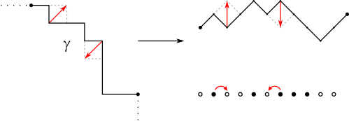
Figure 12: On the left, a portion of region $1$ of an interface $\gamma\in\Omega^{N}_{\text{mic}}$, delimited by the two black dots. On the right, the corresponding path and simple exclusion particle configuration. The mapping is possible if the left-extremity of the interface as well as its length are fixed.

Recall the definition (6.54) of the SSEP part of the Dirichlet form of the contour dynamics. Define then the Dirichlet form $D^{S}_{\ell}$ associated with the SSEP on $\Omega_{\ell}$: for any $g:\Omega_{\ell}\rightarrow\mathbb{R}$,

$$D^{S}_{\ell}(g)=\frac{1}{2|\Omega_{\ell}|}\sum_{\xi\in\Omega_{\ell}}\sum_{\begin{subarray}{c}1\leq u\leq v\leq\ell\\ |u-v|=1\end{subarray}}\frac{1}{2}[\xi_{u}(1-\xi_{v})+\xi_{v}(1-\xi_{u})][g(\xi^{u,v})-g(\xi)]^{2},$$ (6.60)

with $\xi^{u,v}$ the configuration where the state of sites $u,v$ are exchanged. In view of the expression (6.54) of $D_{N}^{S}(g)$, a simple upper-bound and convexity yield:

$$D_{N}^{S}(f) \geq\frac{1}{2}\sum_{x\in(N^{-1}\mathbb{Z})^{2}}\sum_{\gamma\in M(x)}\nu(\gamma)\sum_{\begin{subarray}{c}y\in V(\gamma)\\ x\leq y,\|y-x\|_{1}\leq\ell-1\end{subarray}}c(\gamma,\gamma^{y})\big{[}f^{1/2}(\gamma^{y})-f^{1/2}(\gamma)\big{]}^{1/2}$$

$$\geq\sum_{x\in(N^{-1}\mathbb{Z})^{2}}\nu_{f}(M(x))D^{S}_{\ell}(f_{\ell,x}).$$ (6.61)

Let $\mathcal{U}_{\ell}$ denote the uniform measure on $\Omega_{\ell}$ with associated expectation $E_{\mathcal{U}_{\ell}}$. Using the expressions (6.58)-(6.61), the supremum in (6.55) at time $t\in[0,T]$ can be bounded from above by:

$$\sup_{f\geq 0:\nu_{f}(\mathcal{E})=1}\bigg{\{}\sum_{x\in(N^{-1}\mathbb{Z})^{2}}\nu_{f}(M(x))\Big{[}aG\Big{(}t,x-\frac{2{\bf b}_{1}}{N}\Big{)}E_{\mathcal{U}_{\ell}}\big{[}f_{\ell,x}\phi_{\ell}\big{]}-ND^{S}_{\ell}(f_{\ell,x})\Big{]}\bigg{\}}$$

$$\qquad\leq\sup_{f\geq 0:\nu_{f}(\mathcal{E})=1}\bigg{\{}\sum_{x\in(N^{-1}\mathbb{Z})^{2}}\nu_{f}(M(x))\sup_{g\geq 0:E_{\mathcal{U}_{\ell}}[g]=1}\Big{\{}aG\Big{(}t,x-\frac{2{\bf b}_{1}}{N}\Big{)}E_{\mathcal{U}_{\ell}}[g\phi_{\ell}]-ND^{S}_{\ell}(g)\Big{\}}\bigg{\}}$$

$$\qquad\leq\sup_{f\geq 0:\nu_{f}(\mathcal{E})=1}\bigg{\{}\sum_{x\in(N^{-1}\mathbb{Z})^{2}}\nu_{f}(M(x))a\|G\|_{\infty}\Big{|}\bigg{\}}\sup_{\begin{subarray}{c}g\geq 0:E_{\mathcal{U}_{\ell}}[g]=1\\ D^{S}_{\ell}(g)\leq 2a\|G_{t}\|_{\infty}/N\end{subarray}}E_{\mathcal{U}_{\ell}}[g\phi_{\ell}].$$ (6.62)

The first supremum is bounded by $a\|G_{t}\|_{\infty}$. The problem is therefore now reduced to a one-block estimate for a SSEP of size $\ell$, which is well known (see e.g. [ELS90]): the expectation in (6.62) satisfies:

$$\limsup_{N\rightarrow\infty}\sup_{\begin{subarray}{c}g\geq 0:E_{\mathcal{U}_{\ell}}[g]=1\\ D^{S}_{\ell}(g)\leq 2a\|G_{t}\|_{\infty}/N\end{subarray}}\Big{|}\mathbb{E}_{\mathcal{U}_{\ell}}[g\phi_{\ell}]\Big{|}=O(\ell^{-1}).$$ (6.63)

As the first term in the right-hand side of (6.62) is bounded by $a\|G\|_{\infty}$, the proof of the one block estimate (6.48) is concluded. The two block estimate (6.49) is proven similarly using [ELS90]. ∎

Now that we know that the time integral of ${\bf 1}_{p=2}$ and of the slope at the poles are close, it remains to compute their common value. This is the goal of the next two sections.

6.3.3 A compactness result

In the previous section, the ${\bf 1}_{p=2}$ term was viewed as an occupation number in a SSEP. In this section and the next, we look directly at the pole dynamics, comparing them with well-chosen zero range dynamics in order to compute the value of the time average of ${\bf 1}_{p=2}$. A similar comparison was already used in the proof of the hydrodynamic limit in [LST14], using the monotonicity of the zero temperature Glauber dynamics.

To carry out the comparison with a zero-range process is challenging for the contour dynamics, where monotonicity does not hold. It requires somehow zooming on a neighbourhood of the poles, the definition of which is one of the difficulties. We now present a number of preliminary estimates to that effect. These estimates are very technical. They can be understood as enforcing the fact that the slope around the pole is bounded away from both $0$ and $1$. In terms of zero-range configurations, this will imply that the number of particles in a zero range of size $\ell\in\mathbb{N}^{*}$ is bounded by $C(\ell)$, independently of the scaling parameter $N$, thereby providing a compactness result on the possible zero-range configurations around the pole.

The first estimate is a control of the ${\bf 1}_{p=2}$ term. As shown in Section 6.3.2, this term coincides with the slope around each pole, so that the next result can be understood as proving that poles are typically not flat, a statement made precise afterwards.

Lemma 6.8 (Tail estimate on the flatness of the pole).

For $\gamma\in\Omega^{N}_{\text{mic}}$ with associated droplet $\Gamma$, let $p^{\prime}(\gamma)$ be the number of blocks in $\Gamma$ composing the next level below the north pole, as defined in (6.25). If $C>0$ and $A\geq 2$ is an integer:

$$\limsup_{N\rightarrow\infty}\sup_{\begin{subarray}{c}f\geq 0:E_{\nu}[f]=1\\ D_{N}(f^{1/2})\leq C/N\end{subarray}}\nu_{f}\Big{(}p=2,\gamma^{-,1}\in\Omega^{N}_{\text{mic}},p^{\prime}\geq A\Big{)}\leq\frac{1}{\log A},$$ (6.64)

Proof.

Fix a density $f$ with $D_{N}(f^{1/2})\leq C/N$ throughout. By definition of $\Omega^{N}_{\text{mic}}$, one has $p^{\prime}\geq p$ (recall that $p$ is the number of blocks in the pole). The idea is to estimate $\nu_{f}\big{(}p=2,\gamma^{-,1}\in\Omega^{N}_{\text{mic}},p^{\prime}\geq A\big{)}$ for $A\geq 2$ in terms of $\nu_{f}(p=A,\gamma^{-,1}\in\Omega^{N}_{\text{mic}})$ by a bijection argument similar to the one of Lemma 6.4. The desired bound will then follow from a summation using:

$$\sum_{B\geq 2}\nu_{f}\Big{(}p=B,\gamma^{-,1}\in\Omega^{N}_{\text{mic}}\Big{)}\leq 1.$$ (6.65)

Let us present the aforementioned bijection argument. Fix an integer $A\geq 2$. A curve $\gamma$ in $\big{\{}p=2,\gamma^{-,1}\in\Omega^{N}_{\text{mic}},p^{\prime}\geq A\big{\}}$ can be turned into an element $F(\gamma)$ of $\big{\{}p=A,\gamma^{-,1}\in\Omega^{N}_{\text{mic}}\big{\}}$ as follows. Add up to $A-2$ blocks to the left of the north pole of $\gamma$, with centre at height $z_{1}(\gamma)-\frac{1}{2N}$. If exactly $A-2$ such blocks can be added, an element of $\big{\{}p=A,\gamma^{-,1}\in\Omega^{N}_{\text{mic}}\}$ has been created. If $B<A-2$ blocks only can fit to the left of the pole, add the remaining $A-2-B$ blocks to the right of the pole. The mapping $F$ is illustrated on Figure 13.

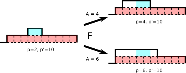
Figure 13: The mapping $F$ for different values of $A$. Here, there are $p^{\prime}=10$ blocks with centre at height $z_{1}-\frac{3}{2N}$, in red and delimited by dashed lines. The two cyan blocks mark the position before and after the mapping by $F$.

Since $p^{\prime}\geq A$, the above procedure always makes sense. Moreover, the mapping $F$ is nearly bijective in the following sense. Label each of the $p^{\prime}$ blocks with centre at height $z_{1}(\gamma)-\frac{3}{2N}$ from $1$ to $p^{\prime}$, starting from the left. We shall say that a block $C$ in the pole is above the block of label $i$ if the centre of $C$ has the same abscissa as the centre of the block of label $i$. Then:

• assume the pole of $\gamma\in\big{\{}p=2,\gamma^{-,1}\in\Omega^{N}_{\text{mic}},p^{\prime}\geq A\big{\}}$ is above the blocks with labels $n,n+1$ with $1\leq n\leq A-1$, and denote this event by $P=\{n,n+1\}$. The procedure described above turns each such curve $\gamma$ into the same $F(\gamma)\in\{p=A,\gamma^{-,1}\in\Omega^{N}_{\text{mic}}\}$ whatever $1\leq n\leq A-1$, and this $F(\gamma)$ is the curve with north pole composed of the blocks above those with labels $1,...,A$. Let $\{P=\{1,...,A\}\}$ refer to the set of such $F(\gamma)$.

• If instead the first block in the pole of $\gamma$ is above a block with label $n\geq A$, an event written $P\geq A$, then the pole of the resulting curve $F(\gamma)$ starts with the block above the one with label $n-(A-2)>1$, and deleting the leftmost $A-2$ blocks in the pole of $F(\gamma)$ transforms it back into $\gamma$.

In terms of the mapping $F$, the previous two cases can be rewritten as follows: for each $n\leq A-1$,

$$F\Big{(}\Big{\{}p=2,\gamma^{-,1}\in\Omega^{N}_{\text{mic}},p^{\prime}\geq A,P=\{n,n+1\}\Big{\}}\Big{)}=\Big{\{}p=A,\gamma^{-,1}\in\Omega^{N}_{\text{mic}},P=\{1,...,A\}\Big{\}},$$ (6.66)

and, more generally writing $\{P\geq n\}$ (resp.: $\{P\leq n\}$) for the events that all blocks in the pole are above blocks with labels at least (resp.: at most) $n$:

$$F\Big{(}\Big{\{}p=2,\gamma^{-,1}\in\Omega^{N}_{\text{mic}},p^{\prime}\geq A,P\geq A\Big{\}}\Big{)}=\Big{\{}p=A,\gamma^{-,1}\in\Omega^{N}_{\text{mic}},P\geq 2\Big{\}}.$$ (6.67)

The event on the right-hand side describes all curves with $p=A$ and a pole that only contains blocks above blocks with labels at least $2$, and is disjoint from the event on the right-hand side of (6.66).
Notice moreover that the mapping $F$ leaves the equilibrium measure $\nu$ invariant, since the length of $\gamma\in\Omega^{N}_{\text{mic}}$ and $F(\gamma)$ are the same. As a result:

$$\nu\Big{(} p=2,\gamma^{-,1}\in\Omega^{N}_{\text{mic}},p^{\prime}\geq A\Big{)}=\nu\Big{(}P\leq A-1,p=2,\gamma^{-,1}\in\Omega^{N}_{\text{mic}},p^{\prime}\geq A\Big{)}$$

$$\hskip 113.81102pt+\nu\Big{(}P\geq A,p=2,\gamma^{-,1}\in\Omega^{N}_{\text{mic}},p^{\prime}\geq A\Big{)}$$

$$\qquad=(A-1)\nu\Big{(}P=\{1,...,A\},\gamma^{-,1}\in\Omega^{N}_{\text{mic}}\Big{)}+\nu\Big{(}P\geq 2,p=A,\gamma^{-,1}\in\Omega^{N}_{\text{mic}}\Big{)}.$$ (6.68)

Each of the above two events contains only curves with $p=A$, thus:

$$\nu\Big{(}p=2,\gamma^{-,1}\in\Omega^{N}_{\text{mic}},p^{\prime}\geq A\Big{)}\leq(A-1)\nu\Big{(}p=A,\gamma^{-,1}\in\Omega^{N}_{\text{mic}}\Big{)}.$$ (6.69)

If valid under $\nu_{f}$, the estimate (6.69) would be enough to obtain (6.64), as we now explain in the $f\equiv 1$ case. Fix an integer $B\geq 2$, and apply (6.69) to each $A\in\{2,...,B\}$ to find:

$$1\geq\sum_{A=2}^{B}\nu\Big{(}p=A,\gamma^{-,1}\in\Omega^{N}_{\text{mic}}\Big{)}\geq\sum_{A=2}^{B}\frac{1}{A-1}\nu\Big{(}p=2,\gamma^{-,1}\in\Omega^{N}_{\text{mic}},p^{\prime}\geq A\Big{)}.$$ (6.70)

For $\ell\geq 2$, let $H_{\ell}=\sum_{n=2}^{\ell}(n-1)^{-1}$, $H_{1}:=0$ and integrate the right-hand side of the last equation by parts to find:

$$1\geq\nu\Big{(}p=2,\gamma^{-,1}\in\Omega^{N}_{\text{mic}},p^{\prime}\geq B\Big{)}H_{B}+\sum_{A=2}^{B-1}H_{A}\nu\Big{(}p=2,\gamma^{-,1}\in\Omega^{N}_{\text{mic}},p^{\prime}=A\Big{)}$$ (6.71)

Equation (6.64) when $f\equiv 1$ follows (in fact also at each $N$ and not just when $N$ is large):

$$\limsup_{N\rightarrow\infty}\nu\Big{(}p=2,\gamma^{-,1}\in\Omega^{N}_{\text{mic}},p^{\prime}\geq B\Big{)}\leq H_{B}^{-1}\leq\frac{1}{\log B}.$$ (6.72)

To obtain (6.64) for a general $\nu$-density $f$, let us now prove that, up to an error that vanishes for $N$ large, (6.69) holds also under $\nu_{f}$. The idea is that the application of the mapping $F$, defined below (6.65), requires changing a number of blocks that is independent from $N$ in a given curve curve, so that $f(\gamma)$ and $f(F(\gamma))$ are close when $\gamma\in\big{\{}p=2,\gamma^{-,1}\in\Omega^{N}_{\text{mic}},p^{\prime}\geq A\big{\}}$.
We prove it for the $\{P=\{1,...,A\},\gamma^{-,1}\in\Omega^{N}_{\text{mic}}\}$ term in (6.69), the $P\geq 2$ term is similar. The method is similar to the one used in Lemma 6.4: we relate the two probabilities under $\nu_{f}$ through the mapping $F$, up to an error term that is then expressed in terms of the Dirichlet form of $f^{1/2}$. Start from:

$$(A-1)\nu_{f} \Big{(}P=\{1,...,A\},\gamma^{-,1}\in\Omega^{N}_{\text{mic}}\Big{)}$$

$$\qquad=(A-1)\sum_{\tilde{\gamma}\in\Omega^{N}_{\text{mic}}}{\bf 1}_{\tilde{\gamma}\in F(\{P\leq A-1,p=2,\gamma^{-,1}\in\Omega^{N}_{\text{mic}},p^{\prime}\geq A\})}\nu(\tilde{\gamma})f\tilde{(}\gamma).$$ (6.73)

Each of the curve $\tilde{\gamma}$ is the image by $F$ of $(A-1)$ different curves in $\{p=2,\gamma^{-,1}\in\Omega^{N}_{\text{mic}},P\leq A-1,p^{\prime}\geq A\}$, so that:

$$(A-1)\nu_{f} \Big{(}P=\{1,...,A\},\gamma^{-,1}\in\Omega^{N}_{\text{mic}}\Big{)}$$

$$=\sum_{\tilde{\gamma}\in\Omega^{N}_{\text{mic}}}{\bf 1}_{\tilde{\gamma}\in F\big{(}\big{\{}P\leq A-1,p=2,\gamma^{-,1}\in\Omega^{N}_{\text{mic}},p^{\prime}\geq A\big{\}}\big{)}}\nu(\tilde{\gamma})f(\tilde{\gamma})\sum_{\gamma\in\{p=2,\gamma^{-,1}\in\Omega^{N}_{\text{mic}},P\leq A-1,p^{\prime}\geq A\}}{\bf 1}_{F(\gamma)=\tilde{\gamma}}$$

$$=\sum_{\gamma\in\big{\{}p=2,\gamma^{-,1}\in\Omega^{N}_{\text{mic}},P\leq A-1,p^{\prime}\geq A\big{\}}}\nu(\gamma)f(F(\gamma)).$$ (6.74)

The last line uses the fact that $F$ does not change the measure $\nu$: $\nu(F(\gamma))=\nu(\gamma)$. Adding and subtracting appropriate terms, (6.74) can be written as:

$$(A-1)\nu_{f} \Big{(}P=\{1,...,A\},\gamma^{-,1}\in\Omega^{N}_{\text{mic}}\Big{)}=\sum_{\gamma\in\big{\{}p=2,\gamma^{-,1}\in\Omega^{N}_{\text{mic}},P\leq A-1,p^{\prime}\geq A\big{\}}}\nu(\gamma)\big{[}f^{1/2}(F(\gamma))-f^{1/2}(\gamma)\big{]}^{2}$$

$$\qquad+\sum_{\gamma\in\big{\{}p=2,\gamma^{-,1}\in\Omega^{N}_{\text{mic}},P\leq A-1,p^{\prime}\geq A\big{\}}}\nu(\gamma)\big{[}-f(\gamma)+2f^{1/2}(\gamma)f^{1/2}(F(\gamma))\big{]}.$$ (6.75)

Cauchy-Schwarz inequality applied to the terms involving $f^{1/2}(\cdot)f(F(\cdot))^{1/2}$ then yields:

$$\Big{[}(A-1)^{1/2}\nu_{f}\Big{(}P= \{1,...,A\},\gamma^{-,1}\in\Omega^{N}_{\text{mic}}\Big{)}^{1/2}-\nu_{f}\Big{(}P\leq A-1,p=2,\gamma^{-,1}\in\Omega^{N}_{\text{mic}},p^{\prime}\geq A\Big{)}^{1/2}\Big{]}^{2}$$

$$\leq\sum_{\gamma\in\{p=2,\gamma^{-,1}\in\Omega^{N}_{\text{mic}},P\leq A-1,p^{\prime}\geq A\}}\nu(\gamma)\big{[}f^{1/2}(F(\gamma))-f^{1/2}(\gamma)\big{]}^{2}.$$ (6.76)

It remains to bound the right-hand side of (6.76) in terms of the Dirichlet form. Decompose the passage from $\gamma$ to $F(\gamma)$ into single-block flips: $\gamma=\gamma_{0}\rightarrow\gamma_{1}\rightarrow...\rightarrow\gamma_{A-2}=F(\gamma)$, and apply Cauchy-Schwarz inequality to find:

$$\sum_{\gamma\in\{p=2,\gamma^{-,1}\in\Omega^{N}_{\text{mic}},P\leq A-1,p^{\prime}\geq A\}} \nu(\gamma)\big{[}f^{1/2}(F(\gamma))-f^{1/2}(\gamma)\big{]}^{2}$$ (6.77)

$$\leq(A-2)\sum_{\gamma\in\{p=2,\gamma^{-,1}\in\Omega^{N}_{\text{mic}},P\leq A-1,p^{\prime}\geq A\}}\nu(\gamma)\sum_{j=1}^{A-2}\big{[}f^{1/2}(\gamma_{j})-f^{1/2}(\gamma_{j-1})\big{]}^{2}.$$

Each move above is authorised in the contour dynamics, at rate $1/2$. A given curve corresponding to one of the $\gamma_{j}$ can occur at most $A-1$ times in all paths $\gamma\rightarrow F(\gamma)$ for $\gamma\in\big{\{}p=2,\gamma^{-,1}\in\Omega^{N}_{\text{mic}},P\leq A-1,p^{\prime}\geq A\big{\}}$. As a result, and since $\nu(\gamma_{j})=\nu(\gamma)$ for all $1\leq j\leq A-2$:

$$\Big{[}(A-1)^{1/2}\nu_{f}\Big{(}P=\{1,...,A\},\gamma^{-,1}\in\Omega^{N}_{\text{mic}}\Big{)}^{1/2}-\nu_{f} \Big{(}P\leq A-1,p=2,\gamma^{-,1}\in\Omega^{N}_{\text{mic}},p^{\prime}\geq A\Big{)}^{1/2}\Big{]}^{2}$$

$$\leq 4(A-1)^{2}D_{N}(f^{1/2}).$$ (6.78)

Similar computations give the same kind of bound for the second term in (6.69) under $\nu_{f}$:

$$\Big{[}\nu_{f}\Big{(}P\geq 2,p=A,\gamma^{-,1}\in\Omega^{N}_{\text{mic}}\Big{)}^{1/2}-\nu_{f}\Big{(}P\geq A,p=2,\gamma^{-,1}\in\Omega^{N}_{\text{mic}}\Big{)}^{1/2}\Big{]}^{2}\leq 4(A-1)D_{N}(f^{1/2}).$$ (6.79)

Let us use (6.78)-(6.79), to prove that (6.69) still holds under $\nu_{f}$ with a small error in $N$ (recall that $D_{N}(f^{1/2})\leq C/N$). Equation (6.78) yields:

$$\nu_{f}\Big{(}P\leq A-1, p=2,\gamma^{-,1}\in\Omega^{N}_{\text{mic}},p^{\prime}\geq A\Big{)}$$

$$\leq(A-1)\nu_{f}\Big{(}P=\{1,...,A\},\gamma^{-,1}\in\Omega^{N}_{\text{mic}}\Big{)}+C(A)\big{[}D_{N}(f^{1/2})^{1/2}+D_{N}(f^{1/2})\big{]}$$

$$\leq(A-1)\nu_{f}\Big{(}P=\{1,...,A\},\gamma^{-,1}\in\Omega^{N}_{\text{mic}}\Big{)}+C(A)N^{-1/2},$$ (6.80)

where the constant $C(A)>0$ changes between inequalities. Similarly, (6.79) yields:

$$\nu_{f}\Big{(}P\geq A,p=2,\gamma^{-,1}\in\Omega^{N}_{\text{mic}}\Big{)} \leq\nu_{f}\Big{(}P\geq 2,p=A,\gamma^{-,1}\in\Omega^{N}_{\text{mic}}\Big{)}+C(A)N^{-1/2},$$ (6.81)

whence the following counterpart of (6.69) for $\nu_{f}$:

$$\nu_{f}\Big{(}p=2,\gamma^{-,1}\in\Omega^{N}_{\text{mic}},p^{\prime}\geq A\Big{)} =\nu_{f}\Big{(}p=2,\gamma^{-,1}\in\Omega^{N}_{\text{mic}},P\leq A-1\Big{)}$$

$$\qquad+\nu_{f}\Big{(}P\geq A,p=2,\gamma^{-,1}\in\Omega^{N}_{\text{mic}}\Big{)}$$

$$\leq(A-1)\nu_{f}\Big{(}p=A,\gamma^{-,1}\in\Omega^{N}_{\text{mic}}\Big{)}+C(A)N^{-1/2}.$$ (6.82)

Equation (6.82) is sufficient to conclude the proof of the upper bound as in the $f\equiv 1$ case, see (6.70) to (6.72). Indeed, the bound in (6.72) requires only the use of $A$ independent from $N$, so that $C(A)N^{-1/2}$ vanishes when $N$ is large. We therefore conclude the proof here. ∎

In the next two lemmas, we use the bound of Lemma 6.8 to control the number of columns in a curve as a function of the vertical distance to the north pole (Lemma 6.9) as well as, conversely, the vertical distance to the north pole as a function of the number of blocks (Lemma 6.10).

More precisely, let $\gamma\in\Omega^{N}_{\text{mic}}\cap\mathcal{E}$. For each $n\in\mathbb{N}^{*}$, the line $y=z_{1}(\gamma)-n/N$ contains a certain number of horizontal edges in $\gamma$ (recall that $z_{1}$ is the ordinate of the highest points in $\gamma$, defined in (6.26)). Let $\ell(n)$ be the number of these edges to the right of $L_{1}$, and $\ell(-n)$ the number of edges to the left of $L_{1}$. Define also $\ell(0):=p(\gamma)-2$. For $N$ large enough, $\gamma\in\Omega^{N}_{\text{mic}}\cap\mathcal{E}$ implies that each of the $\ell(i)$, $|i|\leq n\ll N$ are well defined, see Figure 14.

Lemma 6.9 (Width of a curve at depth $n$ below the north pole).

For $n\in\mathbb{N}^{*},C>0,A\geq 2$,

$$\forall|i|\leq n,\qquad\limsup_{N\rightarrow\infty}\sup_{\begin{subarray}{c}f\geq 0:E_{\nu}[f]=1\\ D_{N}(f^{1/2})\leq C/N\end{subarray}}\nu_{f}\Big{(}\mathcal{E},\ell(i)\geq A\Big{)}\leq\frac{e^{2\beta}}{(A+1)\log(A+2)}.$$ (6.83)

As a result, the numbers $w_{n}^{+}=2+\sum_{i=0}^{n}\ell(i)$ and $w^{-}_{k}=\sum_{i=1}^{n}\ell(-i)$ of blocks with centres at height $z_{1}(\gamma)-N^{-1}(n+1/2)$ in a droplet $\Gamma$ associated to $\gamma\in\mathcal{E}$, respectively to the right/to the left of $L_{1}$ (see Figure 14), satisfy:

$$\limsup_{N\rightarrow\infty}\sup_{\begin{subarray}{c}f\geq 0:E_{\nu}[f]=1\\ D_{N}(f^{1/2})\leq C/N\end{subarray}}\nu_{f}\Big{(}\mathcal{E},w^{\pm}_{n}\geq n^{2}\Big{)}\leq\frac{3e^{2\beta}}{\log n}.$$ (6.84)

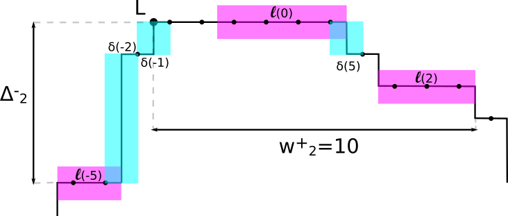
Figure 14: Definition of the $\delta(\pm i),\ell(\pm i),\Delta^{\pm}_{n},w^{\pm}_{n}$. Here $w^{+}_{2}=10$, the number of blocks to the right of $L_{1}$ with centre at height $z_{1}-\frac{5}{2N}$. The small black dots mark the centre of each horizontal edge. The shaded areas highlight which edges make up the represented $\ell(\pm i),\delta(\pm i)$. Here, $\ell(-2)=\delta(-3)=0$.

Proof.

Equation (6.84) follows from (6.83) by a union bound. Let us prove (6.83) by recursion on $|i|\leq n$. The set $\mathcal{E}$ is not stable under the contour dynamics around the poles. Rather than work directly with $\mathcal{E}$, it is convenient to consider a subset that has this stability property. Introduce then the set $Q_{n}$ of curves for which there is some room below the pole:

$$Q_{n}:=\Big{\{}\gamma\in\Omega^{N}_{\text{mic}}:[R_{1}(\gamma)-L_{2}(\gamma)]\cdot{\bf b}_{2}>\frac{n}{N},[R_{1}(\gamma)-R_{4}(\gamma)]\cdot{\bf b}_{2}>\frac{n}{N}\Big{\}}.$$ (6.85)

Note the factor $1/N$ due to the fact that elements of $\Omega^{N}_{\text{mic}}$ are rescaled by definition. For large enough $N\in\mathbb{N}^{*}$, $\mathcal{E}\subset Q_{n}$. Fix one such $N$, $C>0$ and a density $f$ for $\nu$ with $D_{N}(f^{1/2})\leq C/N$ throughout. For $\ell(0)$, one has by Lemma 6.4, using the identity $a-b=(\sqrt{a}-\sqrt{b})(\sqrt{a}+\sqrt{b})$ for $a,b\geq 0$ and bounding the probability below by $1$:

$$\Big{|}\nu_{f}\Big{(} p=2,\gamma^{-,1}\in\Omega^{N}_{\text{mic}},p^{\prime}\geq A+2\Big{)}-E_{\nu_{f}}\Big{[}(p-1)e^{-2\beta}{\bf 1}_{p\geq A+2}\Big{]}\Big{|}$$ (6.86)

$$\quad\leq\big{(}2D_{N}(f^{1/2})\big{)}^{1/2}\Big{[}2+\big{(}2D_{N}(f^{1/2})\big{)}^{1/2}\Big{]}\leq C^{\prime}N^{-1/2},\qquad C^{\prime}=4C+2\sqrt{2C}.$$

Recall that $p=\ell(0)+2$ by definition. Thus:

$$(A+1)\nu_{f}\Big{(}Q_{n},\ell(0)\geq A\Big{)} \leq e^{2\beta}E_{\nu_{f}}\big{[}(\ell(0)+1)e^{-2\beta}{\bf 1}_{\ell(0)\geq A}\big{]}$$

$$=e^{2\beta}E_{\nu_{f}}\big{[}(p-1)e^{-2\beta}{\bf 1}_{p\geq A+2}\big{]}.$$ (6.87)

Equation (6.83) follows for $i=0$ via (6.86):

$$(A+1)\nu_{f}\Big{(}Q_{n},\ell(0)\geq A\Big{)} \overset{\eqref{eq_lien_l_0_p}}{\leq}e^{2\beta}\nu_{f}\Big{(}p=2,\gamma^{-,1}\in\Omega^{N}_{\text{mic}},p^{\prime}\geq A+2\Big{)}+\frac{e^{2\beta}C^{\prime}}{N^{1/2}}$$

$$\overset{\eqref{eq_tail_to_prove_for_compactness_pis_2}}{\leq}\frac{e^{2\beta}}{\log(A+2)}+o_{N}(1).$$ (6.88)

In particular, the result for $i=0$ holds for curves in $\mathcal{E}$. Now assume that, for some integer $i$ with $|i|<n$:

$$\limsup_{N\rightarrow\infty}\sup_{\begin{subarray}{c}f\geq 0:E_{\nu}[f]=1\\ D_{N}(f^{1/2})\leq C/N\end{subarray}}\nu_{f}\Big{(}Q_{n},\ell(i)\geq A\Big{)}\leq\frac{e^{2\beta}}{(A+1)\log(A+2)}.$$ (6.89)

For definiteness, assume $i\geq 0$. To show (6.89) for $i+1$, we are going to prove:

$$\nu_{f}\Big{(}Q_{n},\ell(i+1)\geq A\Big{)}=\nu_{f}\Big{(}Q_{n},\ell(i+1)\geq 0,\ell(i)\geq A\Big{)}+O\big{(}D_{N}(f^{1/2})^{1/2}+D_{N}(f^{1/2})\big{)}.$$ (6.90)

Equation (6.90) implies (6.83) up to $i+1$, since $\mathcal{E}\subset Q_{n}$ for large $N$, and the Dirichlet form vanishes. The idea behind (6.90) is the following. Take a curve $\gamma\in\{\ell(i+1)\geq A\}\cap Q_{n}$ (see Figure 14 for a representation of $\ell(i)$). One can then add at least $A$ blocks to $\Gamma$ with centre at height $z_{1}(\gamma)-N^{-1}(i+1/2)$, one above each of the edges ensuring $\ell(i+1)\geq A$. This bijectively yields a curve $F^{\prime}(\gamma)\in Q_{n}$ with $\ell(i)\geq A$, and $\gamma$ and $F^{\prime}(\gamma)$ have the same length. The two events on either side of (6.90) thus have the same $\nu$-measure.
Under $\nu_{f}$, though, the two events in (6.90) may have different probability. However, the mapping $\gamma\mapsto F^{\prime}(\gamma)$ can be decomposed into a chain of $A$ curves $\gamma=\gamma_{1}\rightarrow...\rightarrow\gamma_{A}=F^{\prime}(\gamma)$, each differing from the previous one by a single block. Each curve $\gamma_{j},j\leq A$ appears at most $A+1$ times when effecting the procedure for all curves in $\{\ell(i+1)\geq A\}\cap Q_{n}$. The cost of turning $\gamma$ into $F^{\prime}(\gamma)$ under $\nu_{f}$ is then estimated by the Dirichlet form in a very similar fashion to the bijection argument of Lemma 6.8, so we give no more details. ∎

The next lemma controls the depth at fixed horizontal distance to the pole. For $n\in\mathbb{N}^{*}$ and $|i|\leq n$, define $\delta(i)$ as the number of vertical edges with abscissa $L_{1}\cdot{\bf b}_{1}+\frac{i+1}{N}$ that belong to either region 4 (if $i\leq 0$) or region 1 ($i\geq 0$), see Figure 14. We fix $\delta_{0}=0$, corresponding to the fact that the pole contains at least two horizontal edges.

Lemma 6.10 (Height of a column at fixed distance to the pole).

For $n\in\mathbb{N}^{*}$ and $C>0,A\geq 1$,

$$\forall 1\leq i,j\leq n,\qquad\limsup_{N\rightarrow\infty}\sup_{\begin{subarray}{c}f\geq 0:E_{\nu}[f]=1\\ D_{N}(f^{1/2})\leq C/N\end{subarray}}\nu_{f}\Big{(}\mathcal{E},\delta(i)\geq A,\delta(-j)\geq A\Big{)}\leq e^{-2\beta(A-1)}.$$ (6.91)

Let $\Delta^{\pm}_{n}=\sum_{i=1}^{n}\delta(\pm i)$ be the number of vertical edges counted in a curve when starting from the point $L_{1}+\frac{{\bf b}_{1}}{N}$ and counting $n+1$ horizontal edges to the right (for $\Delta^{+}_{n}$) or to the left (for $\Delta^{-}_{n}$), see Figure 14. Then, for $\beta>1$:

$$\limsup_{N\rightarrow\infty}\sup_{\begin{subarray}{c}f\geq 0:E_{\nu}[f]=1\\ D_{N}(f^{1/2})\leq C/N\end{subarray}}\nu_{f}\Big{(}\mathcal{E},\Delta^{+}_{n}\geq n(1+\log n),\Delta^{-}_{n}\geq n(1+\log n)\Big{)}\leq\frac{1}{n^{2\beta-2}}=o_{n}(1).$$ (6.92)

Proof.

Let $n\in\mathbb{N}^{*}$ be fixed. Equation (6.92) follows from (6.91) by a union bound. The proof of (6.91) resembles that of Lemma 6.9. We first treat the case $i=j=1$. $\{\delta(1)\geq A,\delta(-1)\geq A\}$ is the event that the north pole is atop a column wide of two blocks, and high of $A$ blocks, the highest two blocks being those in the pole. With each $\gamma\in\{\delta(1)\geq A,\delta(-1)\geq A\}$ associate a curve $\tilde{F}(\gamma)\in\{\delta(1)\geq 1,\delta(-1)\geq 1\}$ in which the north pole has been shrunk $A-1$ times. $\tilde{F}(\gamma)$ has length $|\gamma|-2(A-1)$, thus has higher equilibrium probability. In fact, if $\gamma^{-q}$ denotes the curve $\gamma$ in which the highest $q\in\mathbb{N}^{*}$ groups of two blocks have been deleted, $\tilde{F}$ is a bijection between the sets $\big{\{}\delta(1)\geq A,\delta(-1)\geq A,\gamma^{-(A-1)}\in\Omega^{N}_{\text{mic}}\big{\}}$ and $\big{\{}\delta(1)\geq 1,\delta(-1)\geq 1\big{\}}$, and:

$$\nu\Big{(}\delta(1)\geq A,\delta(-1)\geq A,\gamma^{-(A-1)}\in\Omega^{N}_{\text{mic}}\Big{)}=e^{-2\beta(A-1)}\nu\Big{(}\delta(1)\geq 1,\delta(-1)\geq 1\Big{)}.$$ (6.93)

In the same way as in Lemma 6.8, (6.93) holds under $\nu_{f}$ for any $\nu$-density $f$, up to a term bounded by $o_{N}(1)$ and involving the Dirichlet form as in Lemma 6.9, which quantifies the cost of consecutively deleting the two blocks in the pole of a curve $A-1$ times. As a result:

$$\sup_{\begin{subarray}{c}f\geq 0:E_{\nu}[f]=1\\ D_{N}(f^{1/2})\leq C/N\end{subarray}}\nu_{f}\Big{(}\delta(1)\geq A,\delta(-1)\geq A,\gamma^{-(A-1)}\in\Omega^{N}_{\text{mic}}\Big{)}\leq e^{-2\beta(A-1)}+O\big{(}N^{-1/2}\big{)}.$$ (6.94)

As $\mathcal{E}\subset\{\gamma^{-(A-1)}\in\Omega^{N}_{\text{mic}}\}$ for all large enough $N$, (6.91) holds for $i=j=1$.

To prove (6.91) for each $(i,j)\in\{1,...,n\}$, let us first prove it for $j=1$, $i>1$. As for Lemma 6.9, it is convenient to not work directly with $\mathcal{E}$, which does not have nice stability properties under the contour dynamics, but with the set $\tilde{Q}_{n}$, defined by:

$$\tilde{Q}_{n}:=\Big{\{}\gamma\in\Omega^{N}_{\text{mic}}:\big{[}L_{1}(\gamma)-R_{4}(\gamma)\big{]}\cdot{\bf b}_{1}>\frac{n}{N},\big{[}L_{2}(\gamma)-R_{1}(\gamma)\big{]}\cdot{\bf b}_{1}>\frac{n}{N}\Big{\}}.$$ (6.95)

We claim that, for each $C>0$:

$$\limsup_{N\rightarrow\infty}\sup_{\begin{subarray}{c}f\geq 0:E_{\nu}[f]=1\\ D_{N}(f^{1/2})\leq C/N\end{subarray}}\Big{|}\nu_{f}\Big{(}\tilde{Q}_{n},\delta(i)\geq A,\delta(-1)\geq A\Big{)}-\nu_{f}\Big{(}\tilde{Q}_{n},\delta(i-1)\geq A,\delta(-1)\geq A\Big{)}\Big{|}=0.$$ (6.96)

The idea is the same as in Lemma 6.9. The set $\tilde{Q}_{n}$ ensures that $\delta(i),|i|\leq n$ are well defined and involve only edges in region $4$ ($i\leq 0$) or $1$ ($i\geq 0$). In particular, $\mathcal{E}\subset\tilde{Q}_{n}$ for large enough $N$. A curve in $\tilde{Q}_{n}$ with $\delta(i)\geq A$ is then transformed into one with $\delta(i-1)\geq A$ by deleting $A$ blocks with centres at abscissa $L_{1}\cdot{\bf b}_{1}-\frac{i}{N}+\frac{1}{2N}$. These deletions are SSEP moves, which do not change the length of the curve. Their cost is estimated in terms of the Dirichlet form, which vanishes with $N$.
Iterating (6.96) from $i$ to $1$ and using (6.94) yields (6.91) for the couple $(i,-1)$. Now if $j\neq 1$, the same argument applies to go from $-j$ to $-1$. This concludes the proof of (6.91). ∎

6.3.4 Value of the slope at the pole

We now have all prerequisites to prove that the motion of the north pole imposes a particle density of $e^{-\beta}$ on each side, as stated in Lemma 6.11. The proof relies in a central way on the fact that the contour dynamics around the pole is irreducible, owing to the $e^{-2\beta}$ regrowth updates. These updates are the main difference with the zero temperature stochastic Ising model, and this irreducibility is the main technical reason for the introduction of the parameter $\beta$.

Lemma 6.11.

Let $\beta>1$. For each $T,\delta>0$ and each test function $G\in\mathcal{C}$,

$$\limsup_{N\rightarrow\infty}\frac{1}{N}\log\mathbb{P}^{N}_{\beta}\bigg{(} \gamma^{N}_{\cdot}\in E([0,T],\mathcal{E});$$

$$\bigg{|}\frac{1}{T}\int_{0}^{T}G(t,L_{1}(\gamma^{N}_{t}))\big{(}{\bf 1}_{p=2}-e^{-\beta}\big{)}dt\bigg{|}\geq\delta\bigg{)}=-\infty.$$ (6.97)

The claim is also valid under $\mathbb{P}^{N}_{\beta,H}$ for $H\in\mathcal{C}$ by Corollary 6.2.

Proof.

The proof only deals with $G\equiv 1$ and $H\equiv 0$. Generalisations to $\mathbb{P}^{N}_{\beta,H}$ follow as in the proof of Lemma 6.7, and we explain how to include a test function $G$ in Remark 6.12. Integer parts are systematically omitted, and we drop the superscript $N$ for microscopic curves and trajectories.
The proof is structured as follows. We first use Lemma 6.5 to project the dynamics inside $\mathcal{E}$. The compactness results provided by Section 6.3.3 are then incorporated to the probability in (6.97). This enables us to define a proper frame around the pole. After conditioning to this frame, the quantity to estimate in (6.97) can be retrieved from an equilibrium computation, which is the last step of the proof.

Let $\phi={\bf 1}_{p=2}-e^{-\beta}$. By Markov inequality and Lemma 6.5, the left-hand side of (6.97) without the limits is bounded from above, for each $a>0$ by:

$$-a\delta T+C\beta+\int_{0}^{T}\sup_{f\geq 0:\nu_{f}(\mathcal{E})=1}\Big{\{}aE_{\nu_{f}}[\phi]-ND_{N}(f^{1/2})\Big{\}}dt.$$ (6.98)

It is therefore enough to estimate the supremum in (6.98) at each time (in the present case it is time-independent, see however Remark 6.12).

Step 1: definition of a suitable frame around the pole.
The first step consists in writing the expectation in (6.98) as a quantity that depends only on the dynamics around the pole. The idea is to compare the contour dynamics to a zero-range process with two species of particles. The number of particles is given by the height difference between consecutive columns around the pole. The species is determined by the sign of the height difference. This process is irreducible and its invariant measure can be made explicit. More is said on this dynamics below, see also Figure 16. To make such a comparison, we define a frame around the pole, in which to study the pole dynamics. This is done as follows.

Fix an integer $n\in\mathbb{N}^{*}$, which will be the typical size of the frame around the pole. In the following, for a curve $\gamma\in\Omega^{N}_{\text{mic}}\cap\mathcal{E}$, we talk of blocks at level $q\in\mathbb{N}$ to denote all blocks in $\Gamma$ with centre at height $z_{1}(\gamma)-N^{-1}(q+1/2)$, see Figure 15. With this notation, blocks at level $0$ correspond to blocks in the poles.
Consider the following partition of $\Omega^{N}_{\text{mic}}\cap\mathcal{E}$. For any curve $\gamma\in\Omega^{N}_{\text{mic}}\cap\mathcal{E}$, let $h_{n}(\gamma)$ be the smallest integer such that the number of blocks in $\Gamma$ (the droplet delimited by $\gamma$) at level $z_{1}-N^{-1}\big{(}h_{n}(\gamma)+\frac{1}{2}\big{)}$ is strictly larger than $n$ (see Figure 15):

$$h_{n}(\gamma)=\min\big{\{}q\in\mathbb{N}:N_{q}(\gamma)>n\},$$ (6.99)

where:

$$N_{q}(\gamma)=\Big{|}\Big{\{}\text{blocks in }\Gamma\text{ at level }q,\text{ i.e. with centre at height }z_{1}(\gamma)-\frac{(q+1/2)}{N}\Big{\}}\Big{|}.$$ (6.100)

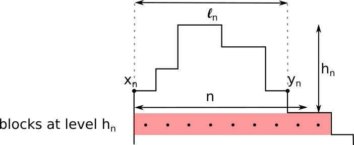
Figure 15: Definition of $h_{n},\ell_{n}$ and $x_{n},y_{n}$ for a given curve. The first level of blocks with width strictly larger than $n$ corresponds to the filled area. In this case there are $n+1$ such blocks, with centres indicated by black dots. The number $\ell_{n}$ of blocks in the last level containing at most $n$ blocks is equal here to $n-1$. The portion of the curve affected by the ZRP dynamics (see Figure 16 below) is delimited by dashed lines and the segment $[x_{n},y_{n}]$.

These objects are well defined for elements of $\Omega_{\text{mic}}^{N}\cap\mathcal{E}$ as soon as $N$ is large enough compared to $n$, which we henceforth assume. Let $x_{n}(\gamma)\leq y_{n}(\gamma)\in V(\gamma)$ denote the extremal vertices of level $h_{n}(\gamma)-1$, i.e. the last level of $\Gamma$ with at most $n$ blocks; and let $\ell_{n}=\ell_{n}(\gamma)$ denote the number of blocks of this level (see Figure 15):

$$\ell_{n}(\gamma):=N\|y_{n}(\gamma)-x_{n}(\gamma)\|_{1}.$$ (6.101)

The rescaling by $N$ comes from the fact that $x_{n}(\gamma),y_{n}(\gamma)$ are points of $(N^{-1}\mathbb{Z})^{2}$. The quantity $\ell_{n}(\gamma)$ is thus an integer. For $2\leq\ell\leq n$, consider the set:

$$M_{\ell}=\big{\{}\gamma\in\Omega^{N}_{\text{mic}}\cap\mathcal{E}:\ell_{n}(\gamma)=\ell\big{\}}.$$ (6.102)

Then $(M_{\ell})_{2\leq\ell\leq n}$ is a disjoint family which partitions $\Omega^{N}_{\text{mic}}\cap\mathcal{E}$ by construction. The expectation in (6.98) thus reads, for each $\nu$-density $f$ supported on $\mathcal{E}$:

$$E_{\nu_{f}}[\phi]=\sum_{2\leq\ell\leq n}E_{\nu_{f}}[{\bf 1}_{M_{\ell}}\phi].$$ (6.103)

At this point, the splitting of curves in the different $M_{\ell}$ in (6.103) suffers from two flaws. On the one hand, the width $\ell$, which will correspond to the number of sites in a zero-range process, may be independent of $n$. This makes a local equilibrium argument impossible to apply. On the other hand, the pole may be macroscopically higher than the points $x_{n}(\gamma),y_{n}(\gamma)$. The point is thus to find diverging sequences $h_{\max}(n),\ell_{\min}(n)$ such that, for any $C>0$:

$$\limsup_{N\rightarrow\infty}\sup_{\begin{subarray}{c}f\geq 0:E_{\nu}[f]=1\\ D_{N}(f^{1/2})\leq C/N\end{subarray}} \nu_{f}\Big{(}\gamma\in\mathcal{E},h_{n}(\gamma)\geq h_{\max}(n)\text{ or }\ell_{n}(\gamma)\leq\ell_{\min}(n)\Big{)}=o_{n}(1).$$ (6.104)

Lemmas 6.9-6.10 enable the construction of such sequences, as we now explain.

Consider first the height $h_{n}(\gamma)$, defined in (6.99). Then either $h_{n}(\gamma)=0$, which corresponds to having at least $n$ blocks in the north pole $P$: $p(\gamma)\geq n$. Or $h_{n}(\gamma)\geq 1$, and there are strictly less than $n$ blocks at level $h_{n}(\gamma)-1$, thus strictly less than $n$ blocks on either sides of $L_{1}$ at this level. Recalling from Lemma 6.10 that $\Delta^{+}_{n}(\gamma)$ (resp.: $\Delta^{-}_{n}(\gamma)$) is the number of vertical edges between the pole and the first point at horizontal distance $n+1$ of $L_{1}+\frac{{\bf b}_{1}}{N}$ on the left (resp.: the right), we find:

$$h_{n}(\gamma)-1\leq\min\big{\{}\Delta^{+}_{n}(\gamma),\Delta^{-}_{n}(\gamma)\big{\}}.$$ (6.105)

Using Lemma 6.9 in the first case and Lemma 6.10 in the second, we obtain, for each $C>0$:

$$\limsup_{N\rightarrow\infty}\sup_{\begin{subarray}{c}f\geq 0:E_{\nu}[f]=1\\ D_{N}(f^{1/2})\leq C/N\end{subarray}}\nu_{f}\Big{(}\gamma\in\mathcal{E},h_{n}(\gamma)\geq h_{\max}(n)\Big{)}=o_{n}(1),\quad h_{\max}(n):=n(1+\log n).$$ (6.106)

We now turn to an estimate of the number of blocks $\ell_{n}=\ell_{n}(\gamma)$ at level $h_{n}(\gamma)-1$. Recalling the definition of the widths $w^{\pm}$ from Lemma 6.9, notice first the identity:

$$\forall\gamma\in\Omega^{N}_{\text{mic}}\cap\mathcal{E},\qquad\ell_{n}(\gamma)=w^{+}_{h_{n}-1}(\gamma)+w^{-}_{h_{n}-1}(\gamma).$$ (6.107)

Let us use (6.107) and a bound on $h_{n}$ to estimate $\ell_{n}$. Let $a_{n}>0$ to be chosen later, fix $C>0$ and a $\nu$-density $f$ with $D_{N}(f^{1/2})\leq C/N$. According to (6.107), one has:

$$\Big{\{}\gamma\in\mathcal{E},\ell_{n}(\gamma)\leq a_{n}\Big{\}}\subset\Big{\{}\gamma\in\mathcal{E},w^{-}_{h_{n}-1}(\gamma)\leq a_{n}\Big{\}}\cap\Big{\{}\gamma\in\mathcal{E},w^{+}_{h_{n}-1}(\gamma)\leq a_{n}\Big{\}}.$$ (6.108)

Consider e.g. $w^{-}_{h_{n}-1}$. Suppose that the path from $L_{1}$ to the left extremity of level $h_{n}-1$ contains at most $a_{n}$ horizontal edges. If one travels a horizontal distance $a_{n}$ to the left of $L_{1}$, it must then be that at least $h_{n}-1$ vertical edges have been encountered, so that:

$$\Big{\{}\gamma\in\mathcal{E}:w^{-}_{h_{n}-1}(\gamma)\leq a_{n}\Big{\}}\subset\Big{\{}\gamma\in\mathcal{E}:\Delta^{-}_{a_{n}}(\gamma)\geq h_{n}(\gamma)-1\Big{\}}.$$ (6.109)

To bound the probability of the event $\{\ell_{n}\leq a_{n}\}$, the idea is then to bound $h_{n}-1$ from below by some $b_{n}$, choose $a_{n}$ such that $\Delta^{-}_{a_{n}}\geq b_{n}$ is unlikely, and conclude from there using (6.108). For $b_{n}>0$ to be chosen later, one has by definition of $h_{n}$:

$$h_{n}\leq b_{n}\quad\Rightarrow\quad w^{-}_{b_{n}}+w^{+}_{b_{n}}>n.$$ (6.110)

Lemma 6.9 controls the width on either side of $L_{1}$: for $b_{n}=\sqrt{n/2}$,

$$\limsup_{N\rightarrow\infty}\sup_{\begin{subarray}{c}f\geq 0:E_{\nu}[f]=1\\ D_{N}(f^{1/2})\leq C/N\end{subarray}} \nu_{f}\big{(}\gamma\in\mathcal{E},h_{n}(\gamma)\leq b_{n}\big{)}$$

$$\leq 2\limsup_{N\rightarrow\infty}\max_{\varepsilon\in\{-,+\}}\sup_{\begin{subarray}{c}f\geq 0:E_{\nu}[f]=1\\ D_{N}(f^{1/2})\leq C/N\end{subarray}}\nu_{f}\Big{(}\gamma\in\mathcal{E},w^{\varepsilon}_{b_{n}}(\gamma)\geq n/2\Big{)}=o_{n}(1).$$ (6.111)

From (6.108) and (6.109) one can therefore write:

$$\Big{\{}\gamma\in\mathcal{E},\ell_{n}\leq a_{n}\Big{\}}\subset\Big{\{}\gamma\in\mathcal{E},\Delta^{-}_{a_{n}}\geq h_{n}-1\Big{\}}\cap\Big{(}\big{\{}h_{n}-1\geq b_{n}\big{\}}\cup\big{\{}h_{n}\leq b_{n}\big{\}}\Big{)}.$$ (6.112)

The event involving $\{h_{n}\leq b_{n}\}$ is estimated through (6.111), so that:

$$\limsup_{N\rightarrow\infty}\sup_{\begin{subarray}{c}f\geq 0:E_{\nu}[f]=1\\ D_{N}(f^{1/2})\leq C/N\end{subarray}} \nu_{f}\Big{(}\gamma\in\mathcal{E},\ell_{n}\leq a_{n}\Big{)}$$

$$\leq\limsup_{N\rightarrow\infty}\sup_{\begin{subarray}{c}f\geq 0:E_{\nu}[f]=1\\ D_{N}(f^{1/2})\leq C/N\end{subarray}}\nu_{f}\Big{(}\gamma\in\mathcal{E},\Delta^{-}_{a_{n}}(\gamma)\geq h_{n}(\gamma)-1\geq b_{n}\Big{)}+o_{n}(1).$$ (6.113)

It remains to choose $a_{n}$ as a function of $b_{n}=\sqrt{n/2}$ so that the probability in the right-hand side of (6.113) vanishes for large $n$. By Lemma 6.10, $\Delta^{-}_{a_{n}}$ is typically smaller than $a_{n}(1+\log(a_{n}))$. It thus suffices to take $a_{n}$ with $a_{n}(1+\log(a_{n}))\leq b_{n}$, e.g. for large enough $n$:

$$a_{n}=(1/2)n^{1/2}/\log n=:\ell_{\min}(n).$$ (6.114)

With this choice of $a_{n}=\ell_{\min}(n)$, (6.113) yields the desired control on $\ell_{n}$:

$$\limsup_{N\rightarrow\infty}\sup_{\begin{subarray}{c}f\geq 0:E_{\nu}[f]=1\\ D_{N}(f^{1/2})\leq C/N\end{subarray}}\nu_{f}\Big{(}\gamma\in\mathcal{E},\ell_{n}(\gamma)\leq\ell_{\min}(n)\Big{)}=o_{n}(1).$$ (6.115)

We now use the bounds (6.106)-(6.115) on $h_{n}$ and $\ell_{n}$ to restrict admissible configurations around the pole, thus concluding the definition of the frame around the pole. Recall that $h_{\max}(n):=n(1+\log n)$ and $\ell_{\min}(n):=(1/2)n^{1/2}/\log n$. From the splitting (6.103) of curves in the different $M_{\ell}$ ($2\leq\ell\leq n$) and the above discussion on bounds of $h_{n},\ell_{n}$, as also $\phi={\bf 1}_{p=2}-e^{-\beta}$ is bounded, (6.98) is bounded from above by:

$$-a\delta T+C\beta+T\ \sup_{f\geq 0:\nu_{f}(\mathcal{E})=1}\Big{\{}a\sum_{\ell_{\min}(n)\leq\ell\leq n}E_{\nu_{f}}\big{[}{\bf 1}_{M_{\ell}}{\bf 1}_{h_{n}\leq h_{\max}(n)}\phi\big{]}-\frac{N}{2}D_{N}(f^{1/2})\Big{\}}+T\omega_{N,n},$$ (6.116)

where $\omega_{N,n}$ satisfies, by (6.106) and (6.115):

$$\limsup_{N\rightarrow\infty}\omega_{N,n}$$

$$\quad\leq a\|\phi\|_{\infty}\limsup_{N\rightarrow\infty}\sup_{\begin{subarray}{c}f\geq 0:E_{\nu}[f]=1\\ D_{N}(f^{1/2})\leq 2\|\phi\|_{\infty}a/N\end{subarray}}\nu_{f}\Big{(}\gamma\in\mathcal{E},h_{n}>h_{\max}(n)\text{ or }\ell_{n}<\ell_{\min}(n)\Big{)}=o_{n}(1).$$ (6.117)

It is thus sufficient to estimate the supremum in (6.116).

Step 2: conditioning and mapping to a two-species zero-range process.

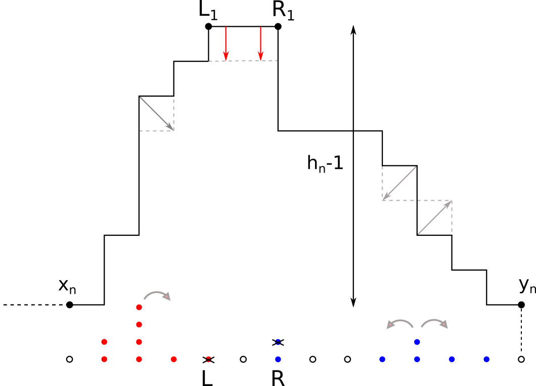
Figure 16: Portion of the interface of a curve around the north pole $[L_{1},R_{1}]$, and associated path and particle configurations. Particles are represented by red dots, antiparticles by blue dots; and empty sites are white with a dark contour. In the particle configuration, the rightmost particle is at site $L$, the leftmost antiparticle at site $R$. The quantity $|\eta_{j}|$ at site $0\leq j\leq\ell$ is the number of particles/antiparticle at site $j$, and $\eta_{j}\geq 0$ for particles, $\eta_{j}\leq 0$ for antiparticles. Here, one has e.g. $\eta_{0}=0,\eta_{2}=4,\eta_{R}=-2$. The height $h_{n}-1$ is the total number of particles (or of antiparticles).
The grey arrows on the particle configuration correspond to jumps allowed by the contour dynamics that conserve the particle number. A move reducing the length of the curve, materialised on the curve by the vertical arrows, corresponds to a particle-antiparticle pair annihilation, represented by the black crosses. No particle creation is represented here.

We now study the expectation in (6.116) on each $M_{\ell}$ for $\ell_{\min}(n)\leq\ell\leq n$, where this set is defined in (6.102). The goal is to obtain a local description of the contour dynamics around the pole. We claim that to each configuration in $M_{\ell}$ corresponds a unique particle configuration in $\Omega_{\ell}=\mathbb{Z}^{\ell+1}$. The mapping goes as follows. If $\gamma\in M_{\ell}$, define, for $0\leq j\leq\ell$, a particle number $\eta_{j}$ corresponding to the height increment at column $j/N$, with column $0$ the one centred on $x_{n}(\gamma)$:

$$\eta_{j}=\varepsilon_{j}\sum_{\begin{subarray}{c}z\in V(\gamma):z\cdot{\bf b}_{1}=x(\gamma)\cdot{\bf b}_{1}+j/N\\ z\cdot{\bf b}_{2}>z_{1}(\gamma)-N^{-1}(h_{n}(\gamma)-1)\end{subarray}}\xi_{z},\quad\varepsilon_{j}=\begin{cases}1&\text{if }j/N\leq L_{1}\cdot{\bf b}_{1},\\ -1&\text{if }j/N>L_{1}\cdot{\bf b}_{1}.\end{cases}$$ (6.118)

In words, $\eta_{j}$ is positive if $j$ is smaller than the abscissa of $L_{1}$, and negative if $j$ is larger. If $\eta_{j}<0$ for some $j$, we say that there are $|\eta_{j}|$ antiparticles at site $j$. The constraint $z\cdot{\bf b}_{2}>z_{1}(\gamma)-N^{-1}(h(\gamma)-1)$ guarantees that only the vertical edges above $x_{n}(\gamma),y_{n}(\gamma)$ are counted as particles. We let $\eta(\gamma)$ denote the unique particle configuration in $\Omega_{\ell}$ associated with $\gamma\in M_{\ell}$ (see Figure 16). Conversely, with each $\eta\in\Omega_{\ell}$ can be associated an interface (in fact, many) in $M_{\ell}$. Note that, as $x_{n}(\gamma)$ and $y_{n}(\gamma)$ have the same ordinate, the number of particles and antiparticles is the same.
In terms of particles, $h_{n}$ corresponds to the number of particles or antiparticles. The event $\{h_{n}\leq h_{\max}(n)\}\cap M_{\ell}$ can thus be rewritten as:

$$W_{\ell}=\{\rho^{\ell}\leq C_{\ell}\},\quad\text{where}\quad\rho^{\ell}=\frac{1}{\ell+1}\sum_{j=0}^{\ell}|\eta_{j}|,\quad C_{\ell}=C_{\ell,n} =\frac{2}{\ell+1}\big{(}h_{\max}(n)-1\big{)}$$

$$=\frac{2n\log n+2(n-1)}{\ell+1}.$$ (6.119)

Let $\ell\in\{\ell_{\min}(n),...,n\}$, $f$ be a $\nu$-density supported on $\mathcal{E}$ with $\nu_{f}(M_{\ell})>0$, and define:

$$\forall\eta\in\Omega_{\ell},\qquad\bar{f}_{\ell}(\eta):=\frac{1}{\nu_{f}(M_{\ell})}\sum_{\gamma\in M_{\ell}:\eta=\eta(\gamma)}\mathcal{Z}_{\beta}^{-1}f(\gamma)\exp\Big{[}-\beta\Big{(}N|\gamma|-\ell-\sum_{j=0}^{\ell}|\eta_{j}|\Big{)}\Big{]}.$$ (6.120)

Define also the probability measure $\bar{\mu}_{\ell}$:

$$\forall\eta\in\Omega_{\ell},\qquad\bar{\mu}_{\ell}(\eta)=\bar{\mathcal{Z}}_{\ell}^{-1}\exp\Big{[}-\beta\ell-\beta\sum_{j=0}^{\ell}|\eta_{j}|\Big{]},$$ (6.121)

where $\bar{\mathcal{Z}}_{\ell}$ is a normalisation factor, and $\sum_{j=0}^{\ell}|\eta_{j}|+\ell$ is the number of edges in the portion of $\gamma$ which is mapped to the particle configuration $\eta$. Though we could factor it out as it is common to all $\eta$, the $e^{-\beta\ell}$ factor in the definition of $\bar{\mu}_{\ell}$ will be convenient later on. In terms of particle configurations, the expectation in (6.116) reads:

$$E_{\nu}\Big{[}f{\bf 1}_{M_{\ell}}{\bf 1}_{h_{n}\leq h_{\max}(n)}\phi\Big{]}=\nu_{f}(M_{\ell})E_{\bar{\mu}_{\ell}}\Big{[}\bar{f}_{\ell}{\bf 1}_{W_{\ell}}\phi\Big{]},$$ (6.122)

so that we know how to estimate the supremum in (6.98) as soon as we can estimate (recall the definition (6.114) of $\ell_{\min}(n)$):

$$\sup_{f\geq 0:\nu_{f}(\mathcal{E})=1}\Big{\{}\sum^{n}_{\ell=\ell_{\min}(n)}a\nu_{f}(M_{\ell})E_{\bar{\mu}_{\ell}}\big{[}\bar{f}_{\ell}{\bf 1}_{W_{\ell}}\phi\big{]}-\frac{N}{2}D_{N}(f^{1/2})\Big{\}},\qquad\phi:={\bf 1}_{p=2}-e^{-\beta}.$$ (6.123)

Step 3: local equilibrium.
We now prove that estimating the supremum in (6.123) reduces to an equilibrium computation. At this stage, the technique is the same as in [KL99]. Denote by $\bar{D}_{\ell}$ the reduced Dirichlet form on $\Omega_{\ell}$, defined as follows. For $\eta\in\Omega_{\ell}$, let $P(\eta)$ denote the vertices making up the "pole" of $\eta$, i.e. $P(\eta)=\{L,...,R\}$, with $L,R$ such that $\eta_{L}$ is the last $\eta_{j}$ that is strictly positive (or $L=0$ if there are no such $\eta_{j}$), and $\eta_{R}$ the first to be strictly negative (or $R=\ell$ if none exist). Let also $p(\eta)=|P(\eta)|-1$. For any two configurations $\eta,\tilde{\eta}\in\Omega_{\ell}$, let $\gamma,\tilde{\gamma}\in M_{\ell}$ respectively be two associated interfaces, and define a jump rate:

$$c(\eta,\tilde{\eta}):=c(\gamma,\tilde{\gamma}),\qquad\text{with }c(\gamma,\tilde{\gamma})\text{ given in Definition }\ref{def_contour_dynamics}.$$ (6.124)

Since the positions of the extremal sites $0$, $\ell$ (corresponding for curves $\gamma$ compatible with a given configuration to the points $x_{n}(\gamma),y_{n}(\gamma)$) are unchanged by dynamical updates involving vertices with ordinate higher than that of $x_{n}(\gamma)$ or $y_{n}(\gamma)$, the last level of $\gamma$ with less than $n$ blocks, which defines the position of $x_{n}(\gamma),y_{n}(\gamma)$, is never modified. The jump rates $c(\eta,\eta^{\prime})$ therefore only depend on $\eta,\eta^{\prime}$, and not on the rest of the curves $\gamma,\gamma^{\prime}$. For any $\bar{\mu}_{\ell}$-density $g$, let $\bar{D}_{\ell}$ denote the associated Dirichlet form:

$$\bar{D}_{\ell}(g^{1/2}) =\frac{1}{2}\sum_{\eta,\tilde{\eta}\in\Omega_{\ell}}\bar{\mu}_{\ell}(\eta)c(\eta,\tilde{\eta})\big{[}g^{1/2}(\tilde{\eta})-g^{1/2}(\eta)\big{]}^{2}.$$ (6.125)

Convexity then yields, recalling that $\ell_{\min}(k)$ is defined in (6.114):

$$D_{N}(f^{1/2})\geq\sum^{n}_{\ell=\ell_{\min}(n)}\nu_{f}(M_{\ell})\bar{D}_{\ell}(\bar{f}_{\ell}^{1/2}).$$ (6.126)

Reinjecting (6.126) into the supremum in (6.123), we see that it is enough to estimate:

$$\sup_{f\geq 0:\nu_{f}(\mathcal{E})=1}\bigg{\{}\sum_{\ell=\ell_{\min}(n)}^{n}\nu_{f}(M_{\ell})\Big{[}aE_{\bar{\mu}_{\ell}}\big{[}\bar{f}_{\ell}{\bf 1}_{W_{\ell}}\phi\big{]}-\frac{N}{2}\bar{D}_{\ell}(\bar{f}_{\ell}^{1/2})\Big{]}\bigg{\}}.$$ (6.127)

We are nearly done with conditioning to a frame where we can compute the expectation in (6.127). The remaining step is to reduce the state space $\Omega_{\ell}=\mathbb{Z}^{\ell+1}$ to something that is compact. By definition of $\bar{f}_{\ell},\bar{\mu}_{\ell},\bar{D}_{\ell}$ in (6.120)-(6.121)-(6.125) respectively, it is enough to delete all jumps that increase the number of particles above what is allowed by $W_{\ell}$ (defined in (6.128)). Indeed, define $\mu_{\ell}$ as a measure on $W_{\ell}$ as follows:

$$\forall\eta\in W_{\ell}=\Big{\{}\rho^{\ell}\leq C_{\ell}=:\frac{2h_{\max}(n)}{\ell+1}\Big{\}},\qquad\mu_{\ell}(\eta):=\mathcal{Z}_{\ell}^{-1}\exp\Big{[}-\beta\ell-\beta\sum_{j=0}^{\ell}|\eta_{j}|\Big{]}=\frac{\bar{\mathcal{Z}}_{\ell}}{\mathcal{Z}_{\ell}}\bar{\mu}_{\ell}(\eta),$$ (6.128)

where $\mathcal{Z}_{\ell}$ is a normalisation factor on $W_{\ell}$. The marginal $\bar{f}_{\ell}$ is correspondingly modified into a $\mu_{\ell}$-density $f_{\ell}$:

$$\forall\eta\in W_{\ell},\qquad f_{\ell}(\eta):=\frac{\mathcal{Z}_{\ell}}{\bar{\mathcal{Z}}_{\ell}}\frac{1}{E_{\bar{\mu}_{\ell}}\big{[}\bar{f}_{\ell}{\bf 1}_{W_{\ell}}\big{]}}\bar{f}_{\ell}(\eta).$$ (6.129)

Finally, the Dirichlet form $D_{\ell}$ for the reduced dynamics (written here in compact form) reads, for any $\mu_{\ell}$-density $g$:

$$D_{\ell}(g^{1/2})=\sum_{\eta,\tilde{\eta}\in W_{\ell}}\mu_{\ell}(\eta)c(\eta,\tilde{\eta})[g^{1/2}(\eta^{\prime})-g^{1/2}(\eta)]^{2}.$$ (6.130)

Since we simply restricted allowed jumps, one has $\bar{D}_{\ell}(\bar{f_{\ell}}^{1/2})\geq D_{\ell}(f_{\ell}^{1/2})E_{\bar{\mu}_{\ell}}[\bar{f}_{\ell}{\bf 1}_{W_{\ell}}]\bar{\mathcal{Z}_{\ell}}/\mathcal{Z}_{\ell}$. Under $\mu_{\ell}$, the supremum to estimate in (6.127) is then bounded from above by:

$$\sup_{f\geq 0:\nu_{f}(\mathcal{E})=1}\bigg{\{}\sum^{n}_{\ell=\ell_{\min}(n)}\nu_{f}(M_{\ell})\frac{\bar{\mathcal{Z}_{\ell}}}{\mathcal{Z}_{\ell}}E_{\bar{\mu}_{\ell}}\big{[}\bar{f}_{\ell}{\bf 1}_{W_{\ell}}\big{]}\Big{[}aE_{\mu_{\ell}}\big{[}f_{\ell}\phi\big{]}-\frac{N}{2}D_{\ell}(f_{\ell}^{1/2})\Big{]}\bigg{\}}$$

$$\leq a\sup_{f\geq 0:\nu_{f}(\mathcal{E})=1}\bigg{\{}\sum^{n}_{\ell=\ell_{\min}(n)}\nu_{f}(M_{\ell})\frac{\bar{\mathcal{Z}_{\ell}}}{\mathcal{Z}_{\ell}}E_{\bar{\mu}_{\ell}}\big{[}\bar{f}_{\ell}{\bf 1}_{W_{\ell}}\big{]}\bigg{[}\sup_{\begin{subarray}{c}g\geq 0:E_{\mu_{\ell}}[g]=1\\ D_{\ell}(g^{1/2})\leq 2a\|\phi\|_{\infty}/N\end{subarray}}E_{\mu_{\ell}}\big{[}g\phi\big{]}\bigg{]}\bigg{\}}$$

$$\leq a\max_{\ell_{\min}(n)\leq\ell\leq n}\bigg{[}\sup_{\begin{subarray}{c}g\geq 0:E_{\mu_{\ell}}[g]=1\\ D_{\ell}(g^{1/2})\leq 2a\|\phi\|_{\infty}/N\end{subarray}}E_{\mu_{\ell}}\big{[}g\phi\big{]}\bigg{]}\times\sup_{f\geq 0:\nu_{f}(\mathcal{E})=1}\bigg{\{}\sum^{n}_{\ell=\ell_{\min}(n)}\nu_{f}(M_{\ell})\frac{\bar{\mathcal{Z}_{\ell}}}{\mathcal{Z}_{\ell}}E_{\bar{\mu}_{\ell}}\big{[}\bar{f}_{\ell}{\bf 1}_{W_{\ell}}\big{]}\bigg{\}}.$$ (6.131)

The second supremum is bounded by $1$. The proof of Lemma 6.11 will therefore be concluded if we can prove that, for fixed $n$ and $N$ large, the supremum on $g$ in the right-hand side of (6.131) is bounded by $o_{n}(1)$ uniformly in $\ell$ with $\ell_{\min}(n)\leq\ell\leq n$.
Fix $\ell\in\{\ell_{\min}(n),...,n\}$. As $W_{\ell}$ is compact, the supremum on $g$ in (6.131) is achieved by a density $g^{N}_{\ell}$ for each $N$. Up to taking a subsequence, by lower semi-continuity of $D_{\ell}$ and continuity of the expectation in (6.131) with respect to weak convergence, we can take the large $N$ limit and restrict ourselves to studying:

$$\sup_{\begin{subarray}{c}g^{\infty}\geq 0:E_{\mu_{\ell}}[g^{\infty}]=1\\ D_{\ell}((g^{\infty})^{1/2})=0\end{subarray}}E_{\mu_{\ell}}[g^{\infty}\phi].$$ (6.132)

By definition of $D_{\ell}$, the zero-range dynamics is irreducible on $W_{\ell}$. This is the major difference between the contour dynamics and the $0$-temperature stochastic Ising model, which motivated the introduction of the temperature-like parameter $\beta$ to allow for regrowth at the poles. Irreducibility means that any $g^{\infty}$ satisfying $D_{\ell}(g^{\infty})=0$ is constant equal to $1$, and we are left with the estimate of:

$$E_{\mu_{\ell}}[\phi]\qquad\text{with}\quad\phi={\bf 1}_{p=2}-e^{-\beta}.$$ (6.133)

Step 4: equilibrium computations
The expectation (6.133) is taken under the equilibrium measure of the zero-range dynamics. Properties of the measure $\mu_{\ell}$ are analysed in Appendix A.3. In particular, it is proven there that, recalling the definition (6.114) of $\ell_{\min}(n)$:

$$\lim_{n\rightarrow\infty}\max_{\ell_{\min}(n)\leq\ell\leq n}\big{|}E_{\mu_{\ell}}[\phi]\big{|}=0.$$ (6.134)

Equation (6.134) concludes the proof of Lemma 6.11 with $G\equiv 1$. ∎

Remark 6.12.

Lemma 6.11 holds for any test function $G\in\mathcal{C}$ and not just $G\equiv 1$: for each $\delta>0$,

$$\limsup_{\varepsilon\rightarrow 0}\limsup_{N\rightarrow\infty}\frac{1}{N}\log\mathbb{P}^{N}_{\beta}\bigg{(} \gamma_{\cdot}\in E([0,T],\mathcal{E});$$ (6.135)

$$\qquad\bigg{|}\frac{1}{T}\int_{0}^{T}G(t,L_{1}(\gamma_{t}))\big{(}{\bf 1}_{p=2}-e^{-\beta}\big{)}dt\bigg{|}\geq\delta\bigg{)}=-\infty.$$

This is proven in the same way as Lemma 6.11, except that curves are further split in terms of the position of the point $x_{n}(\gamma)$ (see Figure 15). Indeed, Feynman-Kac inequality yields the following upper bound as in (6.98):

$$-a\delta T+C\beta+\int_{0}^{T}\sup_{f\geq 0:\nu_{f}(\mathcal{E})=1}\Big{\{}aE_{\nu_{f}}[\phi G(t,L_{1})]-ND_{N}(f^{1/2})\Big{\}}dt.$$ (6.136)

The above supremum is studied at each time $t\leq T$. Since $G$ is bounded, it is still possible to reduce the range of the expectation, so that it is sufficient to estimate the following analogue of (6.116), for each $t\leq T$ and $\nu$-density $f$ supported in $\mathcal{E}$:

$$\sum_{\ell_{\min}(n)\leq\ell\leq k} E_{\nu_{f}}\big{[}{\bf 1}_{M_{\ell}}{\bf 1}_{h_{n}\leq h_{\max}(n)}\phi\ G(t,L_{1})\big{]}$$

$$=\sum_{\ell_{\min}(n)\leq\ell\leq n}E_{\nu_{f}}\big{[}{\bf 1}_{M_{\ell}}{\bf 1}_{h_{n}\leq h_{\max}(n)}{\bf 1}_{x_{n}(\gamma)=x}\phi\ G(t,x_{n})\big{]}+o_{N}(1),$$ (6.137)

with an error term uniform in $f$, accounting for the difference $G(t,L_{1})-G(t,x_{n})$. This error term vanishes for $N$ large due to the conditions $\ell_{n}\leq n$, $h_{n}\leq h_{\max}(n)$ which imply $\|x_{n}-L_{1}\|_{1}\leq C(n)/N$ for some $C(n)>0$ independent of $N$.
Splitting the expectation depending on where $x_{n}$ lies, the first term in (6.137) is bounded by:

$$\sum_{\ell_{\min}(n)\leq\ell\leq n}\sum_{x\in(N^{-1}\mathbb{Z})^{2}}\|G\|_{\infty}\Big{|}E_{\nu_{f}}\big{[}{\bf 1}_{M_{\ell}}{\bf 1}_{h_{n}\leq h_{\max}(n)}{\bf 1}_{x_{n}(\gamma)=x}\phi\big{]}\Big{|}$$ (6.138)

The position of $x_{n}(\gamma)$ is unchanged by the zero-range dynamics, see the discussion following (6.125). As such, the rest of the arguments in the proof of Lemma 6.11 go through unchanged, except that one has to rewrite everything with $x$ fixed, e.g. to consider $M_{\ell,x}=M_{\ell}\cap\{x_{n}(\gamma)=x\}$ instead of $M_{\ell}$, $f_{\ell,x}$ instead of $f_{\ell}$, etc. In particular, the supremum in (6.136) is bounded at each time $t\leq T$ by the following variant of (6.131):

$$a\|G\|_{\infty}\max_{\ell_{\min}(n)\leq\ell\leq n}\bigg{[}\sup_{\begin{subarray}{c}g\geq 0:E_{\mu_{\ell}}[g]=1\\ D_{\ell}(g^{1/2})\leq 2a\|\phi\|_{\infty}\|G\|_{\infty}/N\end{subarray}}\Big{|}E_{\mu_{\ell}}\big{[}g\phi\big{]}\Big{|}\bigg{]}$$

$$\hskip 113.81102pt\times\sup_{f\geq 0:\nu_{f}(\mathcal{E})=1}\bigg{\{}\sum^{n}_{\ell=\ell_{\min}(n)}\sum_{x\in(N^{-1}\mathbb{Z})^{2}}\nu_{f}(M_{\ell,x})\frac{\bar{\mathcal{Z}_{\ell}}}{\mathcal{Z}_{\ell}}E_{\bar{\mu}_{\ell}}\big{[}\bar{f}_{\ell,x}{\bf 1}_{W_{\ell}}\big{]}\bigg{\}}.$$ (6.139)

The estimate of the supremum on the zero-range process is then identical to the one in Lemma 6.11.  $\blacksquare$

The method of proof of Lemma 6.11 can be used to obtain tighter estimates on the slope at the poles. An example is given in the following corollary, used in Appendix B.3 to obtain exponential tightness.

Corollary 6.13 (One and two block estimates for deviations from the average).

Let $\beta>1$. For each $\delta,\eta>0$:

$$\limsup_{q\rightarrow\infty}\limsup_{N\rightarrow\infty}\frac{1}{N}\log\mathbb{P}^{N}_{\beta}\bigg{(} \gamma^{N}_{\cdot}\in E([0,T],\mathcal{E});\frac{1}{T}\int_{0}^{T}{\bf 1}_{|\xi^{\pm,q}_{L_{1}(\gamma^{N}_{t})}-e^{-\beta}|\geq\delta}dt>\eta\bigg{)}=-\infty.$$ (6.140)

and:

$$\limsup_{q\rightarrow\infty}\limsup_{\varepsilon\rightarrow 0}\limsup_{N\rightarrow\infty}\frac{1}{N}\log\mathbb{P}^{N}_{\beta}\bigg{(} \gamma^{N}_{\cdot}\in E([0,T],\mathcal{E});$$

$$\hskip 56.9055pt\frac{1}{T}\int_{0}^{T}{\bf 1}_{|\xi^{\pm,q}_{L_{1}(\gamma^{N}_{t})}-\xi^{\pm,\varepsilon N}_{L_{1}(\gamma^{N}_{t})}|\geq\delta}dt>\eta\bigg{)}=-\infty.$$ (6.141)

Equations (6.140)-(6.141) are valid under $\mathbb{P}^{N}_{\beta,H}$ for $H\in\mathcal{C}$ by Corollary 6.2.

Remark 6.14.

Note that ${\bf 1}_{|\xi^{\pm,q}_{L_{1}}-e^{-\beta}|\geq\delta}$ is simply a cylindrical function, which has average $o_{q}(1)$ under the invariant measure $\nu$. Corollary 6.13 thus says no more than the usual replacement lemmas.  $\blacksquare$

Proof.

Equation (6.141) is a two block estimate which uses only the SSEP part of the dynamics. The method of proof has already been explained in Lemma 6.7.
Consider instead (6.140). The apparent difference with Lemma 6.11 is that, e.g. for $\xi^{+,q}_{L_{1}}$, we need to focus on a frame around the pole which, in addition, has at least $q$ edges to the right of the pole. The fact that it is possible has actually already been proven.
Indeed, it is enough to choose $n=n(q)$ such that e.g. the depth at horizontal distance $q$ on either side of the pole is typically less than $n/2$ in the following sense:

$$\limsup_{N\rightarrow\infty}\sup_{\begin{subarray}{c}f\geq 0:E_{\nu}[f]=1\\ D_{N}(f^{1/2})\leq C/N\end{subarray}}\nu_{f}\Big{(}\mathcal{E},\Delta^{\pm}_{q}\geq n/2\Big{)}=o_{n}(1).$$ (6.142)

By Lemma 6.10, any $n\geq 2q(1+\log q)$ works. It is convenient to have $n$ go to infinity before $q$. The proof of (6.140) is then reduced, as in Lemma 6.11, to an elementary (though more involved) equilibrium computation under the measure $\mu_{\ell}$, defined in (6.128). ∎

Appendix A Projection of the dynamics, replacement lemma and equilibrium estimates

A.1 Projection of the contour dynamics on the good state space

In this section, we prove a general version of Lemma 6.5, which states that the contour dynamics can be projected to the effective state space $\mathcal{E}$. We state and prove a more general result.
Let $(X_{t})_{t\geq 0}$ be a continuous time Markov chain on a finite state space $E$, reversible with respect to a measure $\nu$. If $x_{0}\in E$, let $\mathbb{P}^{X}_{x_{0}},\mathbb{E}^{X}_{x_{0}}$ be the associated probability and expectation. The jump rates of the chain between states $(x,y)\in E^{2}$ are denoted by $c(x,y)$, with associated Dirichlet form $D$:

$$\forall g:E\rightarrow\mathbb{R},\qquad D(g)=\frac{1}{2}\sum_{(x,y)\in E^{2}}\nu(x)c(x,y)\big{[}g(y)-g(x)\big{]}^{2}.$$ (A.1)

Lemma A.1.

Let $B\subset E$ and $x_{0}\in B$. Let also $T>0$ and $\psi:[0,T]\times E\rightarrow\mathbb{R}$ be bounded. Then:

$$\mathbb{E}^{X}_{x_{0}}\bigg{[}{\bf 1}_{\{\forall t\in[0,T],X_{t}\in B\}}\exp\bigg{[}\int_{0}^{T}\psi(t,X_{t})dt\bigg{]}\bigg{]}\leq\frac{1}{\nu(x_{0})}\exp\bigg{[}\int_{0}^{T}\sup_{f\geq 0:\nu_{f}(B)=1}\Big{\{}E_{\nu}\big{[}f\psi(t,\cdot)\big{]}-D(f^{1/2})\Big{\}}dt\bigg{]}.$$

Proof.

Let $(Y_{t})_{t\geq 0}$ be the Markov chain $X$ restricted to live inside $B$ for all time. Write $\mathbb{P}^{Y}_{x},\mathbb{E}^{Y}_{x},x\in B$ for the associated probability and expectation. On $\{\forall t\in[0,T],X_{t}\in B\}$, the two measures $\mathbb{P}^{X}_{x_{0}}$ and $\mathbb{P}^{Y}_{x_{0}}$ are equivalent, and the Radon-Nikodym derivative between $\mathbb{P}^{Y}_{x_{0}}$ and $\mathbb{P}^{X}_{x_{0}}$ up to time $T$ on a trajectory $(X_{t})_{t\leq T}$ taking values in $B$ reads:

$$\frac{d\mathbb{P}^{X}_{x_{0}}}{d\mathbb{P}^{Y}_{x_{0}}}((X_{t})_{t\leq T}) =\exp\bigg{[}\int_{0}^{T}\Big{[}\sum_{y\in B}c(X_{t},y)-\sum_{y\in E}c(X_{t},y)\Big{]}dt-\sum_{t\leq T}\log\bigg{(}\frac{c(X_{t-},X_{t})}{c(X_{t-},X_{t})}\bigg{)}\bigg{]}$$

$$=\exp\bigg{[}-\int_{0}^{T}\sum_{y\notin B}c(X_{t},y)dt\bigg{]}.$$ (A.2)

Letting $Q_{B}(x)=\sum_{y\notin B}c(x,y)$ denote the flux coming out of $B$ from $x$, we find:

$$\mathbb{E}^{X}_{x_{0}}\bigg{[}{\bf 1}_{\{\forall t\in[0,T],X_{t}\in B\}}\exp\bigg{[}\int_{0}^{T}\psi(t,X_{t})dt\bigg{]}\bigg{]}=\mathbb{E}^{Y}_{x_{0}}\bigg{[}\exp\bigg{[}\int_{0}^{T}\Big{\{}\psi(t,Y_{t})-Q_{B}(Y_{t})\Big{\}}dt\bigg{]}\bigg{]}.$$ (A.3)

By reversibility of $X$ with respect to $\nu$, the chain $Y$ is still reversible with respect to $\nu(\cdot\cap B)$:

$$\forall x,y\in B,\qquad c(x,y)\nu(x)=c(y,x)\nu(y).$$ (A.4)

Let us thus apply Feynman-Kac formula after changing the initial condition to $\nu(\cdot\cap B)$:

$$\mathbb{E}^{Y}_{x_{0}}\bigg{[}\exp\bigg{[}\int_{0}^{T}\Big{\{}\psi(t,Y_{t})-Q_{B}(Y_{t})\Big{\}}dt\bigg{]}\bigg{]}$$

$$\hskip 56.9055pt\leq\frac{1}{\nu(x_{0})}\mathbb{E}^{Y}_{\nu(\cdot\cap B)}\bigg{[}\exp\bigg{[}\int_{0}^{T}\Big{\{}\psi(t,Y_{t})-Q_{B}(Y_{t})\Big{\}}dt\bigg{]}\bigg{]}.$$ (A.5)

Consequently:

$$\log\mathbb{E}^{Y}_{x_{0}} \bigg{[}\exp\bigg{[}\int_{0}^{T}\Big{\{}\psi(t,Y_{t})-Q_{B}(Y_{t})\Big{\}}dt\bigg{]}\bigg{]}$$

$$\leq-\log\nu(x_{0})+\log\int_{0}^{T}\sup_{f\geq 0:\nu_{f}(B)=1}\Big{\{}E_{\nu}\Big{[}f\big{(}\psi(t,\cdot)-Q_{B}\big{)}\Big{]}-D_{B}(f^{1/2})\Big{\}}dt.$$ (A.6)

Above, $D_{B}$ is the Dirichlet form of the dynamics restricted to $B$ (compare with (A.1)):

$$\forall g:E\rightarrow\mathbb{R},\qquad D_{B}(g)=\frac{1}{2}\sum_{(x,y)\in B^{2}}\nu(x)c(x,y)\big{[}g(x)-g(y)\big{]}^{2}.$$ (A.7)

This is nearly the statement of Lemma 6.5, except that there the upper-bound involves the original dynamics (in the present case, $X$) rather than the dynamics restricted to $B$. To obtain the desired bound, let us write out $D(f^{1/2})$, defined in (A.1), for a $\nu$-density $f$ with $\nu_{f}(B)=1$:

$$D(f^{1/2}) =\frac{1}{2}\sum_{(x,y)\in B^{2}}\nu(x)c(x,y)\big{[}f^{1/2}(y)-f^{1/2}(x)\big{]}^{2}$$ (A.8)

$$+\frac{1}{2}\sum_{x\in B,y\notin B}\nu(x)c(x,y)f(x)+\frac{1}{2}\sum_{x\notin B,y\in B}\nu(x)c(x,y)f(y).$$

The first line is precisely $D_{B}(f^{1/2})$. By reversibility, each term on the second line of (A.8) is identical and equal to $E_{\nu}\big{(}fQ_{B}/2\big{)}$:

$$E_{\nu}\big{[}fQ_{B}\big{]}=\sum_{x\in B,y\notin B}\nu(x)c(x,y)f(x)=\sum_{x\in B,y\notin B}\nu(y)c(y,x)f(x)=\sum_{x\notin B,y\in B}\nu(x)c(x,y)f(y).$$ (A.9)

As a result, (A.8) becomes:

$$D(f^{1/2})=D_{B}(f^{1/2})+E_{\nu}\big{[}fQ_{B}\big{]}.$$ (A.10)

Inject this equality in the bound (A.6) to find:

$$\log\mathbb{E}^{Y}_{x_{0}} \bigg{[}\exp\bigg{[}\int_{0}^{T}\Big{\{}\phi(t,Y_{t})-Q_{B}(Y_{t})\Big{\}}dt\bigg{]}\bigg{]}$$

$$\leq-\log\nu(x_{0})+\log\int_{0}^{T}\sup_{f\geq 0:\nu_{f}(B)=1}\Big{\{}E_{\nu}\big{[}f\psi(t,\cdot)\big{]}-D(f^{1/2})\Big{\}},$$ (A.11)

which by (A.3) is the claim of Lemma A.1. ∎

A.2 Replacement lemma

In this section, we prove the Replacement Lemma 3.8. Let us first introduce and recall some notations. Fix a time $T>0$ and $A>0$ throughout the section, such that all trajectories considered here will be in the set:

$$\Big{\{}(\gamma^{N}_{t})_{t\leq T}\subset\Omega^{N}_{\text{mic}}\cap\mathcal{E}:\sup_{t\leq T}|\gamma^{N}_{t}|\leq A\Big{\}}.$$ (A.12)

For each $\varepsilon>0$ and $x\in\mathbb{R}^{2}$, recall that $B_{1}(x,\varepsilon)$ is the subset of $\mathbb{R}^{2}$ of points at distance less than $\varepsilon$ to $x$ in $1$-norm. For $\gamma^{N}\in\Omega^{N}_{\text{mic}}$ and $x\in V(\gamma^{N})$, define

$$\phi(\gamma^{N},x)=c_{x}(\gamma^{N})=\frac{1}{2}\big{[}\xi_{x+e^{-}_{x}}(1-\xi_{x})+\xi_{x}(1-\xi_{x+e^{-}_{x}})\big{]}.$$ (A.13)

Recall from (3.3) that $\xi^{\varepsilon N}_{x}$ is the quantity

$$\xi^{\varepsilon N}_{x}=\frac{1}{2\varepsilon N+1}\sum_{y\in V(\gamma^{N})\cap B_{1}(x,\varepsilon)}\xi_{y},$$ (A.14)

and define $\tilde{\phi}$ by:

$$\tilde{\phi}(\rho)=\rho(1-\rho),\qquad\rho\in[0,1].$$ (A.15)

Let $G\in C_{c}(\mathbb{R}_{+}\times\mathbb{R}^{2})$ be a bounded function. By Chebychev exponential inequality and the Projection lemma A.1 applied to the set $E([0,T],\mathcal{E})\cap\big{\{}\sup_{t\leq T}|\gamma^{N}_{t}|\leq A\big{\}}$, Lemma 3.8 holds if, uniformly on $t>0$ and for each $a>0$:

$$\limsup_{\varepsilon\rightarrow 0}\limsup_{N\rightarrow\infty}$$ (A.16)

$$\hskip 14.22636pt\sup_{f\geq 0:\nu_{f}(\mathcal{E}_{A})=1}\Bigg{\{}E_{\nu_{f}}\Bigg{[}a\biggr{\{}\frac{1}{N}\sum_{x\in V(\gamma^{N})}G(t,x)\biggr{[}\phi(\gamma^{N},x)-\tilde{\phi}(\xi_{x}^{\varepsilon N})\biggr{]}\biggr{\}}^{2}\Bigg{]}-ND_{N}(f^{1/2})\Bigg{\}}=0.$$

Above, $\mathcal{E}_{A}$ is the set:

$$\mathcal{E}_{A}:=\mathcal{E}\cap\big{\{}|\gamma|\leq A\big{\}}.$$ (A.17)

Following [ELS90], it is sufficient to prove the following two estimates.

Lemma A.2.

(One and two block estimates)
Let $\varepsilon>0,\ell\in\mathbb{N}^{*}$, and let $(V_{j})_{1\leq j\leq J}$ denote a partition of $\{-\varepsilon N,...,\varepsilon N\}$ in $J$ intervals of length $\ell$ (except maybe the last one that is of size at most $2\ell$), such that $\max V_{j}=\min V_{j+1}-1$ for $j\leq J-1$. For $\gamma^{N}\in\Omega^{N}_{\text{mic}}$, $x\in V(\gamma^{N})$ and $1\leq j\leq J$, let $V_{j}(x)$ be the set of vertices in $B_{1}(x,\varepsilon)\cap V(\gamma^{N})$, with numbering relative to $x$ corresponding to elements of $V_{j}$ (i.e. $x$ corresponds to $0$, $x+{\bf e}^{\pm}_{x}$ to $\pm 1$, etc.). Define also:

$$S(\phi,V_{j}(x)):=\frac{1}{|V_{j}(x)|}\sum_{y\in V_{j}(x)}\phi(\gamma^{N},y),\quad\xi^{V_{j}(x)}:=\frac{1}{|V_{j}(x)|}\sum_{y\in V_{j}(x)}\xi_{y}.$$ (A.18)

For any $a>0$, one has then (one block estimate):

$$\limsup_{\ell\rightarrow\infty}\limsup_{\varepsilon\rightarrow 0}\limsup_{N\rightarrow\infty}\max_{1\leq j\leq J}$$

$$\hskip 28.45274pt\sup_{f\geq 0:\nu_{f}(\mathcal{E}_{A})=1}\bigg{\{}aE_{\nu_{f}}\bigg{[}\frac{1}{N}\sum_{x\in V(\gamma^{N})}\Big{|}S(\phi,V_{j}(x))-\tilde{\phi}(\xi^{V_{j}(x)})\Big{|}^{2}\bigg{]}-ND_{N}(f^{1/2})\bigg{\}}=0,$$ (A.19)

and (two block estimate):

$$\limsup_{\ell\rightarrow\infty}\limsup_{\varepsilon\rightarrow 0}\limsup_{N\rightarrow\infty}\max_{1\leq b,c\leq J}$$

$$\hskip 5.69046pt\sup_{f\geq 0:\nu_{f}(\mathcal{E}_{A})=1}\bigg{\{}aE_{\nu_{f}}\bigg{[}\frac{1}{N}\sum_{x\in V(\gamma^{N})}\Big{|}S(\phi,V_{b}(x))-S(\phi,V_{c}(x))\Big{|}^{2}\bigg{]}-ND_{N}(f^{1/2})\bigg{\}}=0.$$ (A.20)

Proof.

Only microscopic curves occur in this proof, so we drop the superscript $N$ and write $\gamma\in\Omega^{N}_{\text{mic}}$. All distances are in $1$-norm.
The proof is written for a function $\phi$ of range $R\in\mathbb{N}$, i.e. $\phi(\gamma,x)$ depends only on $B_{1}(x,R/N)\cap V(\gamma)$ for each $\gamma\in\Omega^{N}_{\text{mic}}$ and $x\in V(\gamma)$. It in particular applies to (A.13), for which $R=1$. The proof of (A.19)-(A.20) consists in showing that the one and two block estimates for the contour dynamics amount to the same estimates for the SSEP, which are well known [ELS90]. We do it for (A.19), (A.20) is similar. The first step is to discard all points in the sum in (A.19) that are close to the poles, so that the pole dynamics can be neglected.
Define thus, for $u>0$, the set $W^{u}(\gamma)$, which contains all points of $V(\gamma)$ at distance at least $u/N$ from each $L_{i}(\gamma)$, $i\in\{1,...,4\}$ (compare with $V^{u}(\gamma)$, see Figure 8, which contains points at $1$-distance at least $u/N$ from the whole poles rather than their left extremities $u/N$). For any $\gamma\in\Omega^{N}_{\text{mic}}$,

$$\frac{1}{N}\sum_{x\in V(\gamma)}\Big{|}S(\phi,V_{j}(x))-\tilde{\phi}(\xi^{V_{j}(x)})\Big{|}^{2} \leq\frac{1}{N}\sum_{x\in W^{\varepsilon N+R+3}(\gamma)}\Big{|}S(\phi,V_{j}(x))-\tilde{\phi}(\xi^{V_{j}(x)}_{x})\Big{|}^{2}$$

$$\quad+C\|\phi\|_{\infty}\varepsilon.$$ (A.21)

The second term in the right-hand side of (A.21) vanishes for $\varepsilon$ small, and we now estimate the sum. To do so, we split curves between their four regions. The dynamics on each region is then shown to coincide with the SSEP.
To do so, let $1\leq k\leq 4$ and let $M_{k}$ denote the set of all lattice paths compatible with region $1\leq k\leq 4$, defined as follows. For $\gamma\in\Omega^{N}_{\text{mic}}$, let $\gamma_{k}$ denote the part of $\gamma$ that comprises the edges between the vertex $L_{k}+2{\bf e}^{+}_{L_{k}}$, and the vertex before $L_{k+1}$, these two vertices included (with $L_{k+1}:=L_{1}$ when $k=4$). Define then:

$$M_{k}:=\big{\{}\rho\subset(N^{-1}\mathbb{Z})^{2}:\exists\gamma\in\Omega^{N}_{\text{mic}},\gamma_{k}=\rho\big{\}}.$$ (A.22)

One can check that, e.g. when $k=1$, any lattice path on $(N^{-1}\mathbb{Z})^{2}$ allowed to only go right or down and starting above the line $x\cdot{\bf b}_{2}\geq 0$ is an element of $M_{1}$. A similar statement holds for other values of $k$ for the corresponding lattice paths directions.
Define now $\mu_{k}$ as the marginal of the contour measure $\nu=\nu^{N}_{\beta}$ (defined in (2.16)) on $M_{k}$:

$$\forall\rho\in M_{k},\qquad\mu_{k}(\rho)=\frac{e^{-\beta N|\rho|}}{\mathcal{Z}_{k}},\quad\mathcal{Z}_{k}=\sum_{\rho\in M_{k}}e^{-\beta N|\rho|}.$$ (A.23)

Let $f$ be a $\nu$-density supported on $\mathcal{E}_{A}$. Define the corresponding $\mu_{k}$-marginal $f_{k}$:

$$\forall\rho\in M_{k},\qquad f_{k}(\rho)=\frac{1}{\mu_{k}(\rho)}\sum_{\gamma\in\Omega^{N}_{\text{mic}}}{\bf 1}_{\gamma_{k}=\rho}f(\gamma)\nu(\gamma).$$ (A.24)

For $\gamma\in\Omega^{N}_{\text{mic}}$, if $\gamma\setminus\gamma_{k}$ is fixed, then so are all poles. Moreover, if $\gamma$ is in $\mathcal{E}$, then the contour dynamics is local, and the definition of $M_{k}$ implies that updates that modify an edge of $\gamma_{k}$ correspond to SSEP moves. As a result, the Dirichlet form $D_{N}(f^{1/2})$ is bounded from below by convexity according to:

$$D_{N}(f^{1/2})\geq\frac{1}{2}\sum_{k=1}^{4}\sum_{\rho\in M_{k}}\mu_{i}(\rho)\sum_{x\in V(\rho)}c_{x}(\rho)\big{[}f_{k}^{1/2}(\rho^{x,x+{\bf e}^{-}_{x}})-f^{1/2}_{k}(\rho)\big{]}^{2}=:\sum_{k=1}^{4}D_{N}^{k}(f^{1/2}_{k}),$$ (A.25)

where $V(\rho)$ is the set of vertices in $\rho$, and for $k\in\{1,...,4\}$ and a $\mu_{k}$-density $h$, the Dirichlet form $D_{N}^{k}$ corresponding to the SSEP dynamics in region $k$ is given by:

$$D_{N}^{k}(h^{1/2})=\sum_{\rho\in M_{k}}\mu_{k}(\rho)\sum_{x\in V(\rho)}c_{x}(\rho)\big{[}h^{1/2}(\rho^{x,x+{\bf e}^{-}_{x}})-h^{1/2}(\rho)\big{]}^{2}.$$ (A.26)

Let us now see how to use the decomposition on the $M_{k},1\leq k\leq 4$ to estimate the sum appearing in the right-hand side of (A.21). For short, define $\Phi_{j}$ for $1\leq j\leq J$ by:

$$\Phi_{j}(\gamma,x)=\Big{|}S(\phi,V_{j}(x))-\tilde{\phi}(\xi^{V_{j}(x)})\Big{|}^{2},\qquad\gamma\in\Omega^{N}_{\text{mic}},x\in V(\gamma).$$ (A.27)

Note that $\Phi_{j}(\gamma,x)$ depends only on the orientation (horizontal or vertical) of the edges of $\gamma$ at $1$-distance at most $\ell/N$ from $x$, and in particular does not depend on the absolute position of $x$ as a point of $\mathbb{R}^{2}$. We thus only need to keep track of the label of $x$ in a well chosen parametrisation of $\gamma$. We have:

$$(E) :=\sum_{\gamma\in\Omega^{N}_{\text{mic}}\cap\mathcal{E}_{A}}\nu(\gamma)f(\gamma)\frac{1}{N}\sum_{x\in W^{\varepsilon N+R+3}(\gamma)}\Phi_{j}(\gamma,x)$$

$$\ \leq\sum_{k=1}^{4}\sum_{\rho\in M_{k}}\mu_{k}(\rho)f_{k}(\rho)\frac{1}{N}\sum_{x\in W^{\varepsilon N+R}(\rho)}\Phi_{j}(\rho,x),$$ (A.28)

where $\Phi_{j}(\rho,\cdot)$ is defined as in (A.27) replacing $\gamma\in\Omega^{N}_{\text{mic}}$ by a path $\rho\in M_{k}$ ($1\leq k\leq 4$). Since $\phi$ depends only locally on the curve, this is not ambiguous for $x\in W^{\varepsilon N+R}(\rho)$.
So far, we proved that the one block estimate (A.19) holds as soon as:

$$\limsup_{\ell\rightarrow\infty}\limsup_{\varepsilon\rightarrow 0}\limsup_{N\rightarrow\infty}\max_{1\leq j\leq J}$$

$$\hskip 28.45274pt\sup_{f\geq 0:\nu_{f}(\mathcal{E}_{A})=1}\bigg{\{}\sum_{k=1}^{4}\Big{[}a\sum_{\rho\in M_{k}}\mu_{k}(\rho)f_{k}(\rho)\frac{1}{N}\sum_{x\in W^{\varepsilon N+R}(\rho)}\Phi_{j}(\rho,x)-ND_{N}^{k}(f^{1/2}_{k})\Big{]}\bigg{\}}=0.$$ (A.29)

The estimate for each $1\leq k\leq 4$ is identical, so we only do it for $k=1$. Further split paths in $M_{1}$ according to their number of vertices, and let $M_{1}(n)$ be the subset of $M_{1}$ of paths with $n+1$ vertices. All such paths have the same $\mu_{1}$-measure, thus the marginal of $\mu_{1}$ on $M_{1}(n)$ is the uniform measure $U_{n}$ on paths with $n+1$ vertices or, equivalently, by the correspondence expounded in Section 6.3.2 (see Figure 12), of SSEP configurations with $n$ sites. Define $f_{1,n}$ as the corresponding $U_{n}$-marginal of $f_{1}$ on $M_{1}(n)$:

$$\forall\rho\in M_{1}(n),\qquad f_{1,n}(\rho):=E_{\mu_{1}}\big{[}f_{1}{\bf 1}_{M_{1}(n)}\big{]}^{-1}f_{1}(\rho)\mu_{1}(\rho)|M_{1}(n)|\quad\text{if}\quad E_{\mu_{1}}\big{[}f_{1}M_{1}(n)\big{]}>0.$$ (A.30)

It is a density for $U_{n}$, thus convexity of the Dirichlet form yields:

$$D^{1}_{N}(f_{1}^{1/2})\geq\sum_{n\geq 2}E_{\mu_{1}}\big{[}f_{1}{\bf 1}_{M_{1}(n)}\big{]}D^{1}_{N,n}(f_{1,n}^{1/2}),$$ (A.31)

where $D^{1}_{N,n}$ is defined as in (A.26), but with $U_{n}$ instead of $\mu_{1}$, and paths in $M_{1}(n)$ rather than $M_{1}$.
Note also that, as $f$ is supported on $\mathcal{E}_{A}$, $f_{1,n}$ is supported on paths with at most $AN$ edges. In addition, for any $\rho\in M_{1}(n)$ with $n<2\varepsilon N+2R$, $W^{\varepsilon N+R}(\rho)$ is empty. Thus:

$$\sum_{\rho\in M_{1}}\mu_{1}(\rho)f_{1}(\rho)\frac{1}{N}\sum_{x\in W^{\varepsilon N+R}(\rho)}\Phi_{j}(\rho,x)$$

$$\hskip 71.13188pt=\sum_{n=2\varepsilon N+2R}^{AN}E_{\mu_{1}}\big{[}f_{1}{\bf 1}_{M_{1}(n)}\big{]}\frac{1}{|M_{1}(n)|}\sum_{\rho\in M_{1}(n)}\frac{1}{N}\sum_{x\in W^{\varepsilon N+R}(\rho)}\Phi_{j}(\rho,x).$$ (A.32)

Now that paths appearing in (A.32) have fixed length, it is possible to give a numerical label $i\in\{\varepsilon N+R+1,...,n-\varepsilon N-R\}$ to each point in $W^{\varepsilon N+R}(\rho)$, independent from the choice of the path $\rho\in M_{1}(n)$. One can then associate a SSEP configuration $\sigma\in\{0,1\}^{n}$ to each $\rho$ (see Figure 12), and rewrite the quantity $\Phi_{j}(\rho,x)$ for $x\in W^{\varepsilon N+R}(\rho)$ as:

$$\forall x\in W^{\varepsilon N+R}(\rho),\qquad\Phi_{j}(\rho,x)=\Phi(\tau_{i}\sigma),$$ (A.33)

where $i\in\{\varepsilon N+R+1,...,n-\varepsilon N-R\}$ is the label of the point $x$, and $\tau_{i}\sigma(i^{\prime})=\sigma(i^{\prime}-i)$ is the translation operator. The average on $M_{1}$ in (A.32) is then equal to:

$$\sum_{n=2\varepsilon N+2R}^{AN}E_{\mu_{1}}\big{[}f_{1}{\bf 1}_{M_{1}(n)}\big{]}\frac{1}{|M_{1}(n)|}\sum_{\sigma\in\{0,1\}^{n}}g_{1,n}(\sigma)\frac{1}{N}\sum_{i=\varepsilon N+R+1}^{n-\varepsilon N-R}\Phi_{j}(\tau_{i}\sigma).$$ (A.34)

In the last line, $g_{1,n}$ is defined for $\sigma\in\{0,1\}^{n}$ by $g_{1,n}(\sigma)=g_{1,n}(\rho(\sigma))$, with $\rho(\sigma)$ the unique path in $M_{1}(n)$ corresponding to the particle configuration $\sigma$, as represented in Figure 12. In view of (A.29)-(A.31)-(A.34), to prove the one block estimate (A.19), it is sufficient to prove:

$$\limsup_{\ell\rightarrow\infty}\limsup_{\varepsilon\rightarrow 0}\limsup_{N\rightarrow\infty}\max_{1\leq j\leq J}$$

$$\hskip 28.45274pt\max_{n\in\{2\varepsilon N+2R,...,AN\}}\sup_{g\geq 0:E_{U_{n}}[g]=1}\bigg{\{}\frac{a}{N}\ E_{U_{n}}\Big{[}g\sum_{i=\varepsilon N+R+1}^{n-\varepsilon N-R}\Phi_{j}(\tau_{i}\cdot)\Big{]}-ND^{S}_{n}(g^{1/2})\bigg{\}}=0.$$ (A.35)

The notation $D_{n}^{S}$, already used in Section 6, stands for the Dirichlet form associated with a SSEP on $n$ sites. We are left with a usual one block estimate for a SSEP of size $n$, proven e.g. in [ELS90]. The size $n$ of the SSEP becomes irrelevant in the large $N$ limit since only the $2\ell+1$ site closest to each $i$ matter, hence the proof of (A.19). The two block estimate (A.20) is proven similarly. ∎

A.3 Equilibrium estimates at the pole

In this section, we investigate the equilibrium measure $\mu_{\ell}$ (see (6.128)) of the zero-range process at the poles. We prove:

Proposition A.3.

The sequence $(\mu_{\ell})_{\ell}$ satisfies a large deviation principle at speed $\ell$ for the top height of a path (equivalently: the number of particles or of antiparticles) with good, convex rate function given by:

$$\forall u\geq 0,\qquad C(u)=2\beta u-2u\log\big{(}1+1/(2u)\big{)}-\log(1+2u)-\log\big{(}1-e^{-\beta}\big{)}.$$ (A.36)

In particular, recalling that $\ell_{\min}(n):=(1/2)n^{1/2}/\log n$:

$$\lim_{n\rightarrow\infty}\max_{\ell_{\min}(n)\leq\ell\leq n}\big{|}E_{\mu_{\ell}}[\phi]\big{|}=0,\qquad\phi={\bf 1}_{p=2}-e^{-\beta}.$$ (A.37)

Proof.

We say that a path is a north-east path if it goes either up or right, a south-east path if it goes either down or right, and an up-down path if it can be described as the stitching of a south-east path to the right of a north-east path (see Figure 17).
Recall that up-down paths correspond to possible configurations of the neighbourhood of the north pole of microscopic interfaces $\gamma^{N}\in\Omega^{N}_{\text{mic}}$. In contrast, the north-east paths appearing below do not have any interpretation in terms of microscopic interfaces.

We speak alternately of up-down paths or of particle/antiparticle configurations in the proof depending on what is easier to use, the height of a path corresponding to $\sum_{x\leq L_{1}}\eta_{x}=-\sum_{x>L_{1}}\eta_{x}$. Here, the point $L_{1}$ is the left extremity of the pole of an up-down path. This pole and $L_{1}$ for a north-east path are defined analogously to the north pole of a curve $\gamma^{N}\in\Omega^{N}_{\text{mic}}$ and its left extremity $L_{1}(\gamma)$. We similarly write $p$ for the length of the pole of an up-down path.
Fix $\ell_{\min}(n)\leq\ell\leq n$ throughout. Let us first study the probability to observe a given height under $\mu_{\ell}$. There are exactly $\binom{2q+\ell-2}{2q}$ configurations with height $q\in\mathbb{N}$. To see it, notice that this is the number of north-east paths with length $2q+\ell-2$ and $2q$ vertical edges. To each such path $\rho$, one can associate a unique up-down path of length $2q+\ell$ as follows (see also Figure 17).

• Travelling on the path $\rho$ from its origin, stop at the first point at height $q$, call it $X$, and cut the path there, in two parts $\rho_{\leq X}$ and $\rho_{>X}$.

• Add two horizontal edges to $\rho_{\leq X}$ immediately after $X$, call $\rho_{X+2}$ the resulting path.

• Change $\rho_{>X}$ into its symmetrical $\tilde{\rho}_{>X}$ with respect to the horizontal, i.e. change every upwards edge into a downwards one, leaving the horizontal edges unchanged. Stitch the last edge of $\rho_{X+2}$ to the first of $\tilde{\rho}_{>X}$ to obtain an up-down path of height $q$ and length $2q+\ell$.

One easily checks that this mapping is a bijection, mapping the point $X$ onto the left extremity $L_{1}$ of the pole of the up-down path, whence:

$$\forall q\leq h_{\max}(n)=n(1+\log n),\qquad\mu_{\ell}\Big{(}\sum_{j\leq L_{1}}\eta_{j}=q\Big{)}=\binom{2q+\ell-2}{2q}e^{-2\beta q-\beta\ell}/\mathcal{Z}_{\ell}.$$ (A.38)

Let us investigate the dependence of this quantity in $q<h_{\max}(k)$:

$$\mu_{\ell}\Big{(}\sum_{j\leq L_{1}}\eta_{j}=q+1\Big{)}/\mu_{\ell}\Big{(}\sum_{j\leq L_{1}}\eta_{j}=q\Big{)}=e^{-2\beta}\frac{(2q+\ell)(2q+\ell-1)}{(2q+2)(2q+1)}.$$ (A.39)

This quantity increases until some value $q_{c}$ of $q$, given by

$$q_{c}=\frac{1}{2}(e^{\beta}-1)^{-1}\ell+o(\ell)=:u_{c}\ell+o(\ell).$$ (A.40)

In particular, due to the logarithm in the large deviation bounds for the measure $\mu_{\ell}$ that we are trying to prove, only the maximum value of $\binom{2q+\ell-2}{2q}e^{-2\beta q-\beta\ell}$ will matter. One thus needs only consider heights of order $\ell$ in the large $\ell$ limit. For fixed $u>0$, elementary computations give:

$$\frac{1}{\ell}\log\bigg{[}\binom{2\lfloor\ell u\rfloor+\ell-2}{2\lfloor\ell u\rfloor}e^{-2\beta\lfloor\ell u\rfloor-\beta\ell}\bigg{]}=-\beta-2\beta u+2u\log\big{(}1+1/(2u)\big{)}+\log(1+2u)+o_{\ell}(1).$$ (A.41)

Define the function $D(\cdot)$ on $\mathbb{R}^{*}_{+}$ by;

$$\forall u\geq 0,\qquad D(u)=\beta+2\beta u-2u\log\big{(}1+1/(2u)\big{)}-\log(1+2u)\geq 0.$$ (A.42)

From (A.41) and with $u_{c}=\frac{1}{2}(e^{\beta}-1)^{-1}$, we obtain for the normalisation $\mathcal{Z}_{\ell}$:

$$\lim_{\ell\rightarrow\infty}\frac{1}{\beta\ell}\log\mathcal{Z}_{\ell}=\frac{D(u_{c})}{\beta}=1+\frac{1}{\beta}\log\big{(}1-e^{-\beta}\big{)}.$$ (A.43)

We now turn to the large deviation principle for the height of a path. From (A.41) and (A.43), we obtain

$$\frac{1}{\ell}\log\mu_{\ell}\Big{(}\sum_{j\leq L_{1}}\eta_{j}=\lfloor\ell u\rfloor\Big{)}=-(D(u)-D(u_{c}))+o_{\ell}(1),$$ (A.44)

Define the rate function $C(\cdot)$ on $\mathbb{R}^{*}_{+}$ by

$$\forall u\geq 0,\qquad C(u)=D(u)-D(u_{c})\geq 0.$$ (A.45)

The function $C$ is $C^{\infty}$ on $\mathbb{R}^{*}_{+}$, and satisfies:

$$C(u_{c})=0=C^{\prime}(u_{c}),\qquad C^{\prime\prime}(u)=\frac{2}{u+2u^{2}}>0\text{ for each }u>0,$$ (A.46)

so that $C$ is strictly convex, and a good rate function. The large deviation principle follows from (A.44).

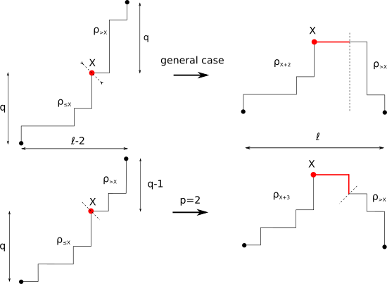
Figure 17: Bijection argument to count the number of up-down paths with height $q$ and length $2q+\ell$, with (bottom figure) or without (top figure) conditions on the size $p$ of the pole. Black dots delimit the extremities of the paths. Without conditions on $p$, an up-down path is obtained by transforming a north-east path with length $2q+\ell-2$ and height $2q$ (top left figure). If $p=2$, then instead the length is $2q+\ell-3$ and height $2q-1$ (bottom left figure). Dashed lines delimit the two portions $\rho_{\leq X}$ and $\rho_{>X}$ of the north-east paths. The red dot is the place at which the initial north-east path is split, and the red, thick lines on the right-hand side are the edges added to the initial path to obtain an up-down configuration with height $q$ and length $2q+\ell$ (with also $p=2$ in the bottom figure).

It remains to prove (A.37). This follows from the large deviations principle (A.44) and the following observation. Constructing a path with $p=2$ and height $q\in\mathbb{N}^{*}$ is done by building a north-east path of length $2q-1+\ell-2$ with $2q-1$ vertical edges, then cutting it as described previously and taking the symmetric part of the path after the first point $X$ at height $q$. The only difference is that one now sticks not just two horizontal edges after $X$, but two horizontal edges followed by a vertical one hanging from below, before stitching back the two parts of the path (see Figure 17). There are thus $\binom{2q+\ell-3}{2q-1}$ configurations with $p=2$ and height $q\in\mathbb{N}^{*}$, and:

$$\mu_{\ell}\Big{(}p=2,\sum_{j\leq L_{1}}\eta_{j}=q\Big{)}=\mathcal{Z}_{\ell}^{-1}e^{-\beta\ell-2\beta q}\binom{2q+\ell-3}{2q-1}=\frac{2q}{2q+\ell-2}\mu_{\ell}\Big{(}\sum_{j\leq L_{1}}\eta_{j}=q\Big{)}.$$ (A.47)

From (A.47), using $(\ell+1)\rho^{\ell}=2\sum_{j\leq L_{1}}\eta_{j}$, the expectation in (A.37) for each $\ell\in\{\ell_{\min}(n),...,n\}$ reads, with $\ell_{\min}(n)=(1/2)n^{1/2}/\log n$:

$$E_{\mu_{\ell}}[\phi] =-e^{-\beta}+\sum_{q\geq 1}\mu_{\ell}\Big{(}p=2,\sum_{j\leq L_{1}}\eta_{j}=q\Big{)}\overset{\eqref{eq_mes_pis2_height_q_is_propto_height_q}}{=}E_{\mu_{\ell}}\bigg{[}\frac{2\sum_{j\leq L_{1}}\eta_{j}}{2\sum_{j\leq L_{1}}\eta_{j}+\ell-2}-e^{-\beta}\bigg{]}.$$ (A.48)

Let $\zeta>0$. The integrand in (A.48) is bounded and, for all $\ell$ large enough,

$$\frac{1}{\ell}\log\mu_{\ell}\Big{(}\frac{1}{\ell}\sum_{j\leq L_{1}}\eta_{j}\notin[u_{c}-\zeta,u_{c}+\zeta]\Big{)}\leq-C(u_{c}+\zeta)/2<0.$$ (A.49)

As a result, since $2u_{c}/(2u_{c}+1)=e^{-\beta}$, the expectation in (A.48) is recast as follows:

$$E_{\mu_{\ell}}[\phi] =E_{\mu_{\ell}}\bigg{[}\bigg{(}\frac{2\ell^{-1}\sum_{j\leq L_{1}}\eta_{j}}{2\ell^{-1}\sum_{j\leq L_{1}}\eta_{j}+1}-e^{-\beta}\bigg{)}{\bf 1}_{u_{c}-\zeta\leq\frac{1}{\ell}\sum_{j\leq L_{1}}\eta_{j}\leq u_{c}+\zeta}\bigg{]}+O(\ell^{-1})$$

$$=O(\zeta)+O(\ell^{-1}).$$ (A.50)

The $O(\zeta)$ is independent of $\ell$, which proves (A.37). ∎

Appendix B Topology results

At the microscopic level, elements of $\Omega^{N}_{\text{mic}}$ are Jordan curves. Macroscopically, however, curves may be non-simple, for instance when the situation of Figure 6 occurs. In this section, we define a topology on trajectories of curves that is both sufficiently weak for exponential tightness to be available (proven in Appendix B.3), yet strong enough for the motion of the poles to be controlled.

B.1 Topological properties of $\Omega$ and $\mathcal{E}$

In this section, we prove topological properties of $\mathcal{E},\Omega$ and characterise Hausdorff convergence. Recall the convention:

$$\forall\gamma,\tilde{\gamma}\in\Omega,\qquad d_{L^{1}}(\gamma,\tilde{\gamma}):=d_{L^{1}}(\Gamma,\tilde{\Gamma})=\int_{\mathbb{R}^{2}}|{\bf 1}_{\Gamma}-{\bf 1}_{\tilde{\Gamma}}|dudv,$$ (B.1)

where $\Gamma,\tilde{\Gamma}$ are the droplets associated with $\gamma,\tilde{\gamma}$ respectively. Let us first introduce useful notations.

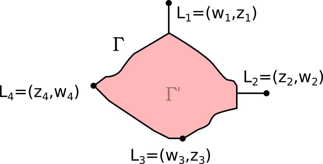
Figure 18: A droplet $\Gamma$ associated with a curve in $\mathcal{E}$ with point-like north and east poles. The left extremities $L_{k}$ ($1\leq k\leq 4$) of the pole are indicated by black dots. Here, for $u,v\in\mathbb{R}$, $(u,v)$ is the point $u{\bf b}_{1}+v{\bf b}_{2}$. The droplet $\Gamma^{\prime}$ corresponds to the red shaded area.

Definition B.1.

For $1\leq k\leq 4$, recall that the $z_{k}=z_{k}(\gamma)$ are the extremal coordinates of a curve $\gamma\in\mathcal{E}$:

$$z_{1}=z_{1}(\gamma)=\sup\{x\cdot{\bf b}_{2}:x\in\gamma\}=L_{1}\cdot{\bf b}_{2},\qquad z_{3}=\inf\{x\cdot{\bf b}_{2}:x\in\gamma\}=L_{3}\cdot{\bf b}_{2},$$

$$z_{2}=\sup\{x\cdot{\bf b}_{1}:x\in\gamma\}=L_{2}\cdot{\bf b}_{1},\hskip 65.44142ptz_{4}=\inf\{x\cdot{\bf b}_{1}:x\in\gamma\}=L_{4}\cdot{\bf b}_{1}.$$ (B.2)

Define the $w_{k}$, $1\leq k\leq 4$, as the other four coordinates of the left extremities $L_{k}$ of each pole: $w_{1}=L_{1}\cdot{\bf b}_{1},w_{2}=L_{2}\cdot{\bf b}_{2}$, etc. It will later be useful to also write $(z_{k}(\Gamma),w_{k}(\Gamma)):=(z_{k}(\gamma),w_{k}(\gamma))$ if $\Gamma$ is the droplet associated with $\gamma$.
Contrary to microscopic curves, macroscopic interfaces may have point-like poles connected to the droplet via a segment (see e.g. $\Gamma^{2}$ in Figure 20 below). It is convenient to introduce the set of curves without such poles. Define thus $\Gamma^{\prime}\subset\Gamma$ as the largest droplet with simple boundary such that $d_{L^{1}}(\Gamma,\Gamma^{\prime})=0$. In other words, $\Gamma^{\prime}$ is the closure of the interior of $\Gamma$ (see Figure 18). Define then $\mathcal{E}^{\prime}\subset\mathcal{E}$ as the set of boundaries of all such droplets:

$$\mathcal{E}^{\prime}:=\{\partial(\Gamma^{\prime}):\gamma=\partial\Gamma\in\mathcal{E}\}.$$ (B.3)

Proposition B.2.

The sets $\Omega$ and $\mathcal{E}$ are closed in the topology associated with the Hausdorff distance $d_{\mathcal{H}}$ between droplets, defined in (2.9). Moreover, $\mathcal{E}$ is closed in $\Omega$ for the volume distance $d_{L^{1}}$, defined in (B.1).
In addition, $\Omega\cap\{|\gamma|\leq\kappa\}$ is compact in Hausdorff topogy (thus $\mathcal{E}\cap\{|\gamma|\leq\kappa\}$ as well) for each $\kappa>0$.

Proof.

If a sequence converges in Hausdorff distance, then it converges in volume distance $d_{L^{1}}$. In particular, $\mathcal{E}$ is a closed subset of $\Omega$ for both the $d_{L^{1}}$ and the Hausdorff distances. Let us thus prove that $\Omega$ is closed in Hausdorff distance.
The Hausdorff distance $d_{\mathcal{H}}$ between non-empty compact sets $A,B\subset\mathbb{R}^{2}$ is equivalently defined by (2.9), and by:

$$\qquad d_{\mathcal{H}}\big{(}A,B)=\max\Big{\{}\sup_{y\in B}\inf_{x\in A}\|x-y\|_{1},\sup_{x\in A}\inf_{y\in B}\|x-y\|_{1}\Big{\}}=d_{\mathcal{H}}\big{(}\partial A,\partial B).$$ (B.4)

From this definition, it is not difficult to see that the extremal coordinates $(z_{k})_{1\leq k\leq 4}$ of a curve are $1$-Lipschitz functions. In particular, if $\lim_{n}d_{\mathcal{H}}(\gamma^{n},\gamma)=0$ for a sequence $(\gamma^{n})\subset\Omega$ and $\gamma\subset\mathbb{R}^{2}$, then the sequences $(z_{k}(\gamma^{n}))_{n}$ of extremal coordinates of the $\gamma^{n}$ converge to $z_{k}(\gamma)$ for each $k$ with $1\leq k\leq 4$ ($z_{k}$ is a Lipschitz function), so that $\gamma$ has finite length and four poles. The fact that $\lim_{n}d_{L^{1}}(\gamma^{n},\gamma)=0$ can then be used to prove that $\gamma$ satisfies Property 2.1, i.e. $\gamma\in\Omega$. This proves the first half of the proposition.

Consider now the second half of the proposition. For $\kappa>0$, $\gamma\in\Omega\cap\{|\gamma|\leq\kappa\}$ implies that $|z_{k}(\gamma)|\leq\kappa/2$ for each $k$ with $1\leq k\leq 4$. Since $\gamma$ surrounds $0$ by Definition 2.2 of $\Omega$, the set $\Omega\cap\{|\gamma|\leq\kappa\}$ is closed in Hausdorff topology in the set of non-empty compact sets in $[-\kappa/2,\kappa/2]^{2}$, which is compact. This concludes the proof. ∎

In the rest of this subsection, we describe the topology put on $\Omega$ (and $\mathcal{E}$), i.e. how to characterise the proximity of two curves. The natural candidate is the Hausdorff distance $d_{\mathcal{H}}$ (recall (B.4)). However, due to the very constrained structure of curves in $\Omega$ (see Property 2.1), in our case a meaningful notion of distance should directly quantify proximity of two curves in terms of the proximity of their volume and of their poles.
Such a distance, topologically equivalent to the Hausdorff distance, is built in Lemma B.4. This distance will be particularly useful to characterise relative compactness at the level of trajectories, in Section B.2.1. Before stating this lemma, let us establish properties of the poles.

Lemma B.3.

• The functional $w_{k}$ ($1\leq k\leq 4$) satisfies $w_{k}\in[z_{k-1},z_{k+1}]$ with the convention $k+1:=1$ if $k=4$ and $k-1:=4$ if $k=1$. It is not continuous in Hausdorff distance, but $w_{1}$ is lower semi-continuous if $k\in\{1,4\}$, upper semi-continuous if $k\in\{2,3\}$. In contrast, $z_{k}$ is 1-Lispchitz with $z_{1},z_{2}\geq 0$, $z_{3},z_{4}\leq 0$ while $\gamma\in\mathcal{E}\mapsto z_{k}(\Gamma^{\prime})$ is lower semi-continuous if $k\in\{1,2\}$, upper semi-continuous if $k\in\{3,4\}$.

• If the Hausdorff distance between two curves in $\mathcal{E}$ is large enough, then at least one of these curves has large length. Formally:

  $$\forall\lambda\geq 2|\gamma^{\text{ref}}|,\forall\gamma,\tilde{\gamma}\in\mathcal{E},\qquad d_{\mathcal{H}}(\gamma,\tilde{\gamma})\geq\lambda\quad\Rightarrow\quad|\gamma|\geq\frac{\lambda}{2}\text{ or }|\tilde{\gamma}|\geq\frac{\lambda}{2}.$$ (B.5)

• Let $\gamma\in\mathcal{E}$ have point-like pole $k$ ($1\leq k\leq 4$). Then, if $(\gamma^{n})_{n}\subset\mathcal{E}$ converges to $\gamma$ in Hausdorff distance,

  $$\lim_{n\rightarrow\infty}\big{\|}L_{k}(\gamma^{n})-L_{k}(\gamma)\big{\|}_{1}\vee\big{\|}R_{k}(\gamma^{n})-R_{k}(\gamma)\big{\|}_{1}=0.$$ (B.6)

  In particular, $w_{k}$ is continuous in Hausdorff distance at each curve $\gamma\in\mathcal{E}$ with point-like pole $k$ ($1\leq k\leq 4$).

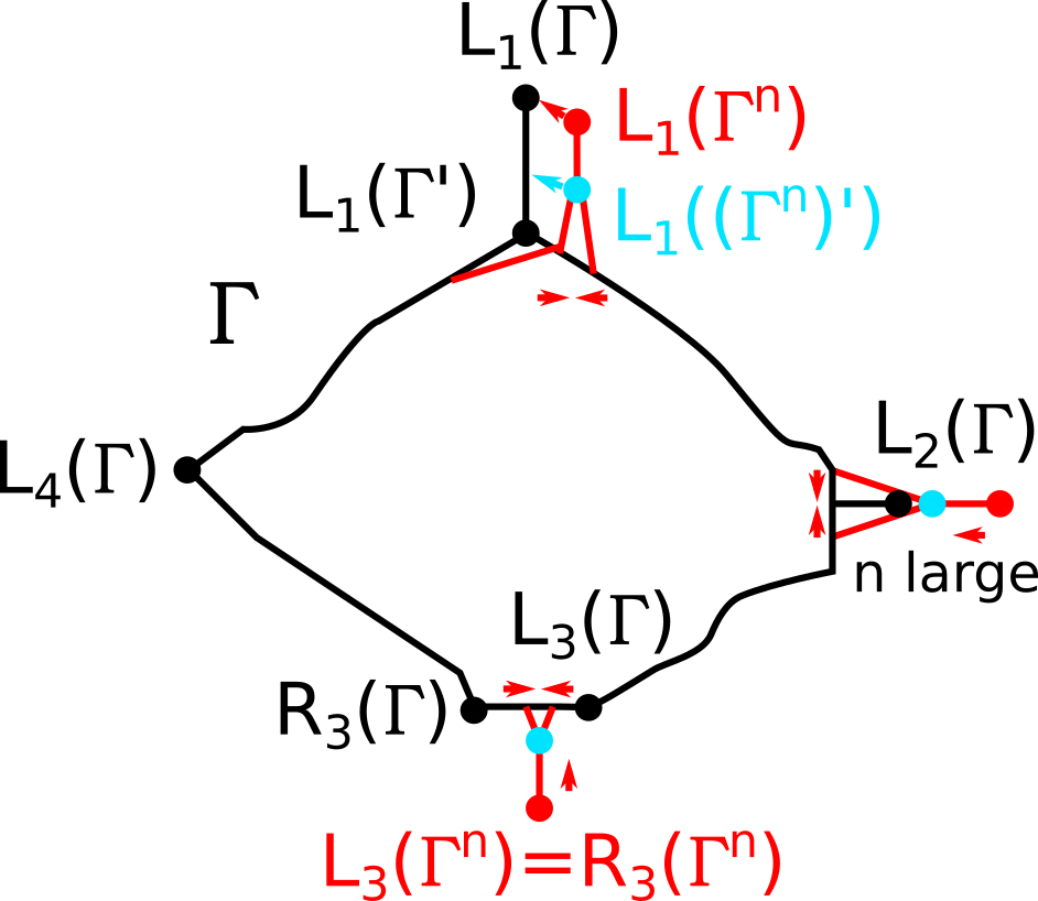
Figure 19: Continuity property of the $z_{k},w_{k}$ and $\gamma\mapsto z_{k}(\Gamma^{\prime})$ for the Hausdorff distance. A droplet $\Gamma$ and an element $\Gamma^{n}$ of a sequence of droplets with boundaries converging in Hausdorff distance to $\partial\Gamma$ (differing from $\Gamma$ in the portions materialised by red lines) are represented. The extremities of the poles of $\Gamma,\Gamma^{n}$ are given by dark dots, and the position of $L_{k}(\Gamma^{\prime}),L_{k}((\Gamma^{n})^{\prime})$ by light blue dots. Arrows indicate the evolution of $\Gamma^{n}$ when $n$ is large. The convergence at each pole illustrates a different possible behaviour.
The droplet $\Gamma$ has point-like pole 1, thus $\lim_{n}L_{1}(\Gamma^{n})=L_{1}(\Gamma)$. However, $\Gamma^{n}$ is chosen in such a way that $\liminf_{n}z_{1}((\Gamma^{n})^{\prime})>z_{1}(\Gamma^{\prime})$.
Similarly, at pole 2 of $\Gamma$, $\Gamma^{n}$ is such that $\lim L_{2}(\Gamma^{n})=L_{2}(\Gamma)$, but $\inf_{n}z_{2}((\Gamma^{n})^{\prime})>z_{2}(\Gamma^{\prime})$: $\gamma\mapsto z_{i}(\Gamma^{\prime})$ is lower semi-continuous if $i\in\{1,2\}$.
At pole $3$, where $L_{3}(\Gamma^{n})=R_{3}(\Gamma^{n})$, it does not hold that $\lim_{n}L_{3}(\Gamma^{n})=L_{3}(\Gamma)$: neither $w_{3}(\Gamma)=L_{3}(\Gamma)\cdot{\bf b}_{1}$ nor $R_{3}(\Gamma)\cdot{\bf b}_{1}$ are the limits of $L_{3}(\Gamma^{n})\cdot{\bf b_{1}}$. The functionals $R_{3}\cdot{\bf b}_{1}$ and $L_{3}\cdot{\bf b}_{1}=w_{3}$ are respectively lower- and upper semi-continuous (while instead $w_{1}=L_{1}\cdot{\bf b}_{1}$ is lower- and $R_{1}\cdot{\bf b}_{1}$ upper semi-continuous, etc.).

Proof.

$\bullet$ For the first point, note that by definition, the $z_{k}$ $(1\leq k\leq 4)$ are the extremal coordinates of points of an interface. E.g. for $k=1$, $z_{4}$ is the lowest abscissa, $z_{2}$ the highest; while $w_{1}$ is the abscissa of the left extremity $L_{1}$ of the north pole. Thus $w_{1}\in[z_{4},z_{1}]$, and similarly for $w_{k}$ for $k\geq 2$.

The lack of continuity of $w_{k}$ is best explained on a picture (see right picture in Figure 20). The idea is the following.
E.g. for the north pole $k=1$, let $\gamma\in\mathcal{E}^{\prime}$ have north pole not reduced to a point: $|P_{1}(\gamma)|>0$. Then one can build two sequences $(\gamma_{1}^{n})_{n}$, $(\gamma^{n}_{2})_{n}$ of curves with point-like north pole, at ordinate $z_{1}(\gamma)+1/n$, and at respective abscissa $w_{1}(\gamma)=L_{1}(\gamma)\cdot{\bf b}_{1}$ and $R_{1}(\gamma)\cdot{\bf b}_{1}\neq w_{1}(\gamma)$. Then $\lim_{n}d_{\mathcal{H}}(\gamma^{n}_{1},\gamma)=0=\lim_{n}d_{\mathcal{H}}(\gamma^{n}_{2},\gamma)$, but $w(\gamma^{n}_{2})$ converges to $R_{1}(\gamma)\cdot{\bf b}_{1}\neq w_{1}(\gamma)$.
That $z_{k}$ is $1$-Lipschitz follows directly from Definition (B.4) of the Hausdorff distance. Note also that $z_{1},z_{2}\geq 0$ and $z_{3},z_{4}\leq 0$, as curves in $\Omega$ must surround the point $0$ by Definition 2.2. Thus upper semi-continuity of $z^{\prime}_{k}:=\gamma\mapsto z_{k}(\Gamma^{\prime})$ ($k\in\{3,4\}$) describes the same phenomenon as lower semi-continuity of $z^{\prime}_{1},z^{\prime}_{2}$. We only prove lower semi-continuity of $z^{\prime}_{1}$ on $\mathcal{E}$. Let $(\gamma^{n})\subset\mathcal{E}$ converges to $\gamma\in\mathcal{E}$. Then $z_{1}^{\prime}\in[z_{3},z_{1}]$, as by definition $z_{1}$ is the largest and $z_{3}$ the smallest ordinate of points in a curve. Since $(z_{1}(\gamma^{n}))_{n},(z_{3}(\gamma^{n}))_{n}$ converge and are therefore bounded, it follows that $(z^{\prime}_{1}(\gamma^{n}))_{n}$ converges up to a subsequence (still written $(z^{\prime}_{1}(\gamma^{n}))_{n}$). Suppose by contradiction that its limit $\bar{z}^{\prime}_{1}$ satisfies $\bar{z}^{\prime}_{1}\leq z^{\prime}(\gamma)-\varepsilon$ for some $\varepsilon>0$. Then, for all large enough $n$:

$$z^{\prime}_{1}(\gamma^{n})\leq z^{\prime}_{1}(\gamma)-\varepsilon/2.$$ (B.7)

The last equation implies that the intersection of the strip $\{(u,v)\in\mathbb{R}^{2}:v\in z^{\prime}_{1}(\gamma)+[-\varepsilon/2,0]\}$ with the droplet $\Gamma^{n}$ associated with $\gamma^{n}$ has vanishing volume when $n$ is large. On the other hand, the volume of this strip intersected with $\Gamma$ (the droplet associated with $\gamma$) is strictly positive. This is absurd, since $\lim_{n}d_{\mathcal{H}}(\gamma^{n},\gamma)=0$ implies $\lim_{n}d_{L^{1}}(\gamma^{n},\gamma)=0$. Thus $\bar{z}^{\prime}_{1}\geq z^{\prime}_{1}(\gamma)-\varepsilon$ for arbitrary $\varepsilon>0$ and the lower semi-continuity.

$\bullet$ Consider now the second point. Let $\lambda\geq 2|\gamma^{\text{ref}}|$ and $\gamma,\tilde{\gamma}\in\mathcal{E}$ with $d_{\mathcal{H}}(\gamma,\tilde{\gamma})\geq\lambda$. This choice of a lower bound for $\lambda$ is made to ensure that curves with length $\lambda/2$ exist in $\mathcal{E}$.
Recall that elements of $\Omega\supset\mathcal{E}$ must contain $0$. If both $|\gamma|,|\tilde{\gamma}|\leq\lambda/2$, it follows that $\gamma,\tilde{\gamma}$ are included in the square $[-\lambda/4,\lambda/4]^{2}$. By Definition (B.4) of the Hausdorff distance, this implies $d_{\mathcal{H}}(\gamma,\tilde{\gamma})\leq\lambda/2$, which is a contradiction.

$\bullet$ For the third point, we treat only the north pole, the others being similar. Let $\gamma\in\mathcal{E}$ have point-like north pole, and $(\gamma^{n})_{n}\subset\mathcal{E}$ converge to $\gamma$ in Hausdorff distance. The key observations are that, on the one hand, the functional $L_{1}\cdot{\bf b}_{2}=R_{1}\cdot{\bf b}_{2}\ (=z_{1})$ is continuous in Hausdorff distance on $\mathcal{E}$ (see the first point of the lemma); while on the other hand $L_{1}\cdot{\bf b}_{1}\ (=w_{1})$ is lower semi-continuous and $R_{1}\cdot{\bf b}_{1}$ is upper semi-continuous (see Figure 19). As a result, and since $\Gamma$ has point-like north pole:

$$L_{1}(\gamma)\cdot{\bf b}_{1}\leq\liminf_{n\rightarrow\infty}L_{1}(\gamma^{n})\cdot{\bf b}_{1}\leq\limsup_{n\rightarrow\infty}R_{1}(\gamma^{n})\cdot{\bf b}_{1}\leq R_{1}(\gamma)\cdot{\bf b}_{1}=L_{1}(\gamma)\cdot{\bf b}_{1}.$$ (B.8)

This concludes the proof of (B.6) for the north pole, and the others are similar. ∎

As announced above Lemma B.3, we may now characterise Hausdorff convergence in terms of the convergence of the volume and of the poles (see Figure 20 and Remark B.5 for heuristics).

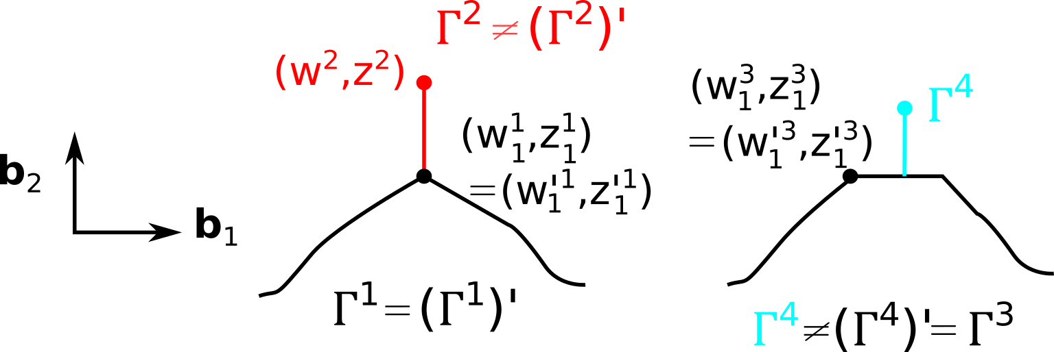
Figure 20: Neighbourhood of the north pole of three droplets $\Gamma^{i}$, $1\leq i\leq 4$ assumed to be identical except in the pictured portion. On the figure, $w^{\prime i}_{1},z^{\prime i}_{1}$ is short for $w_{1}((\Gamma^{i})^{\prime}),z_{1}((\Gamma^{i})^{\prime})$ respectively, and $w^{i}_{1},z^{i}_{1}$ is short for $w_{1}(\Gamma^{i}),z_{1}(\Gamma^{i})$. Recall that e.g. $(\Gamma^{2})^{\prime}$ is the largest droplet with simple boundary contained in $\Gamma^{2}$ (equal here to $\Gamma^{1}$, i.e. $\Gamma^{2}$ without the vertical red line), see also Figure 18.
Convergence to $\Gamma^{1},\Gamma^{2}$ and $\Gamma^{3}$ in Hausdorff distance is equivalent to convergence in volume and for $z_{1}$, i.e. convergence of $w_{1}$ is not needed. Indeed, the droplets $\Gamma^{1}$ and $\Gamma^{3}$ have simple boundaries, so the only missing information is the height of the limiting north pole. For $\Gamma^{2}$ (equal to $\Gamma_{1}$ except for the red part), $\Gamma^{2}\neq(\Gamma^{2})^{\prime}$, however the pole of $(\Gamma^{2})^{\prime}$ is point-like so that $w^{\prime 2}_{1}=w^{2}_{1}$. As $(\Gamma^{2})^{\prime}$ has simple boundary, the situation is the same as for $\Gamma^{1}$.
In contrast, convergence in Hausdorff distance to $\Gamma^{4}$ does require convergence of $w_{1}$. This is because $\Gamma^{4}$ has point-like north pole but $(\Gamma^{4})^{\prime}=\Gamma^{3}$ does not. The control of the lateral position $w^{4}_{1}$ of the pole is thus necessary to converge to $\Gamma^{4}$, and it is not provided by the knowledge of $(\Gamma^{4})^{\prime}=\Gamma^{3}$.

Lemma B.4.

Let $\iota:\mathbb{R}\rightarrow[0,1]$ be a strictly increasing continuous function such that $\iota(0)=0$. Recalling the convention (B.1), consider the distance $\tilde{d}_{\mathcal{H}}$ on $\mathcal{E}$, defined for $\gamma,\tilde{\gamma}\in\mathcal{E}$ and associated droplets $\Gamma,\tilde{\Gamma}$ as:

$$\tilde{d}_{\mathcal{H}}(\gamma,\tilde{\gamma}) =d_{L^{1}}(\Gamma,\tilde{\Gamma})+\sum_{k=1}^{4}\big{|}z_{k}(\Gamma)-z_{k}(\tilde{\Gamma})\big{|}$$

$$\quad+\sum_{k=1}^{4}\iota\Big{(}\max\big{\{}|z_{k}(\Gamma)-z_{k}(\Gamma^{\prime})|,|z_{k}(\tilde{\Gamma})-z_{k}(\tilde{\Gamma}^{\prime})|\big{\}}\Big{)}\big{|}w_{k}(\Gamma)-w_{k}(\tilde{\Gamma})\big{|}.$$ (B.9)

Then $\tilde{d}_{\mathcal{H}}$ and $d_{\mathcal{H}}$ are topologically equivalent on $\mathcal{E}$.

Remark B.5.

The statement of Lemma B.4 is important. Though it is already discussed at length in Figure 20 from another point of view, let us therefore take the time to explain the definition (B.9) of $\tilde{d}_{\mathcal{H}}$.
Note first that all microscopic curves, i.e. elements of $\Omega^{N}_{\text{mic}}$, are simple. For these curves, the function $\iota$ vanishes. It is only useful to control singularities at the poles of elements of $\Omega$.

The volume distance does not control possible singularities at the poles of elements of $\Omega$, whereas the Hausdorff distance does. If a curve $\gamma$ with associated droplet $\Gamma$ is simple in the neighbourhood of its pole $k$ ($1\leq k\leq 4$), then additionally controlling the $z_{k}$ is sufficient to control convergence in Hausdorff distance (the $w_{k}$ are not needed in that case, and are determined by the convergence in volume). This corresponds to $\Gamma^{1}$ in Figure 20.
Similarly, if $\gamma$ is not simple around pole $k$ but $\Gamma^{\prime}$ has point-like pole $k$, then controlling the volume and $z_{k}$ is enough to control convergence in Hausdorff distance (corresponding to $\Gamma^{2}$ in Figure 20). This accounts for the first line in (B.9).

There are two additional situations that $\tilde{d}_{\mathcal{H}}$ should account for. The first situation corresponds to convergence to a curve that does not have point-like pole $k$, for some $1\leq k\leq 4$. In this case, convergence in Hausdorff distance does not imply convergence of $w_{k}$, so $\tilde{d}_{\mathcal{H}}$ should not impose this convergence. This is the role played by the function $\iota$ in the second line of (B.9), which vanishes in that case (this claim is established in the proof of Lemma B.4).
The second situation occurs when the limiting curve $\gamma$ indeed has point-like pole $k$, but $\Gamma^{\prime}$ does not have point-like pole $k$. In this case convergence in Hausdorff distance does require convergence of $w_{k}$ (see $\Gamma^{4}$ on Figure 20). Thus $w_{k}$ is added in the second line of (B.9) (and $\iota$ does not vanish in that situation). This second situation is illustrated for pole 2 of the droplet in Figure 19.  $\blacksquare$

Proof of Lemma B.4.

Let $(\gamma^{n})_{n}\subset\mathcal{E}$ converge to $\gamma\in\mathcal{E}$ for $d_{\mathcal{H}}$, with as usual $(\Gamma^{n})_{n},\Gamma$ the associated droplets. Then $\lim_{n}d_{L^{1}}(\Gamma^{n},\Gamma)=0$, and $(z_{k}(\gamma^{n}))_{n}$ converges to $z_{k}(\gamma)=z_{k}(\Gamma)$ for $1\leq k\leq 4$, as these objects are continuous in Hausdorff distance. Suppose first $z_{k}(\Gamma)=z_{k}(\Gamma^{\prime})$ for each $k$ ($1\leq k\leq 4$). Recall that $z_{k}(\Gamma^{n})\geq z_{k}((\Gamma^{n})^{\prime})$ if $k\in\{1,2\}$, $z_{k}(\Gamma^{n})\leq z_{k}((\Gamma^{n})^{\prime})$ if $k\in\{3,4\}$ by definition, Moreover, $\gamma\in\mathcal{E}\mapsto z_{k}(\Gamma^{\prime})$ is lower semi-continuous for $k\in\{1,2\}$ and upper semi-continuous for $k\in\{3,4\}$) by item 1 of Lemma B.3. The convergence $\lim_{n}z_{k}(\Gamma^{n})=z_{k}(\Gamma)$ then implies $\lim_{n}|z_{k}((\Gamma^{n})^{\prime})-z_{k}(\Gamma^{n})|=0$, thus $\iota$ vanishes in the second line of $\tilde{d}_{\mathcal{H}}(\gamma^{n},\gamma)$, and $\lim_{n}\tilde{d}_{\mathcal{H}}(\gamma^{n},\gamma)=0$.
If instead $z_{k}(\Gamma)>z_{k}(\Gamma^{\prime})$ for some $1\leq k\leq 4$, then $\gamma$ has point-like pole $k$, and $\iota$ is bounded from below at pole $k$. However, a point-like pole $k$ means that $w_{k}$ is a Hausdorff-continuous functional at $\gamma$ by (B.6), thus $\lim_{n}w_{k}(\gamma^{n})=w_{k}(\gamma)$. It follows that $\lim_{n}\tilde{d}_{\mathcal{H}}(\gamma^{n},\gamma)=0$.

Conversely, assume $(\gamma^{n})_{n}\subset\mathcal{E}$ converges to $\gamma\in\Omega$ for $\tilde{d}_{\mathcal{H}}$. Convergence in volume implies that $\gamma\in\mathcal{E}$ by Proposition B.2. Convergence of the $(z_{k}(\gamma^{n}))_{n}$ ($1\leq k\leq 4$) implies convergence of the length $(|\gamma^{n}|)_{n}$, which is in particular bounded by some $C>0$. The set:

$$\mathcal{E}_{C}:=\{\bar{\gamma}\in\mathcal{E}:|\bar{\gamma}|\leq C\}$$ (B.10)

is compact for the Hausdorff distance by Proposition B.2. Let thus $\gamma^{\infty}$ denote a limit point of $(\gamma^{n})_{n}$ for $d_{\mathcal{H}}$, and write $\Gamma,\Gamma^{\infty}$ for the droplets associated with $\gamma,\gamma^{\infty}$ respectively. By continuity of the $z_{k}$ and volume for both $d_{\mathcal{H}}$ and $\tilde{d}_{\mathcal{H}}$, one has:

$$d_{L^{1}}(\gamma,\gamma^{\infty})=0\quad\text{(thus }\Gamma^{\prime}=(\Gamma^{\infty})^{\prime}\text{)},\qquad z_{k}(\gamma)=z_{k}(\gamma^{\infty}),\quad 1\leq k\leq 4.$$ (B.11)

If $z_{k}(\Gamma^{\prime})=z_{k}(\Gamma)$ for each $1\leq k\leq 4$, then by (B.11) the same is true for pole $k$ of $\Gamma^{\infty}$, and $\Gamma=\Gamma^{\infty}$. The only possibility for $\Gamma,\Gamma^{\infty}$ to differ is thus when the situation represented by $\Gamma^{3}$ and $\Gamma^{4}$ in Figure 20 occurs, i.e. when $z_{k}(\Gamma)>z_{k}(\Gamma^{\prime})$ for some $1\leq k\leq 4$ and pole $k$ of $\Gamma^{\prime}$ is not point-like, so that $w_{k}(\gamma)$ may differ from $w_{k}(\gamma^{\infty})$.
However, as soon as $z_{k}(\Gamma)=z_{k}(\Gamma^{\infty})>z_{k}(\Gamma^{\prime})=z_{k}((\Gamma^{\infty})^{\prime})$ for some $1\leq k\leq 4$, then $\gamma,\gamma^{\infty}$ have point-like pole $k$, thus $w_{k}$ is in particular continuous in Hausdorff distance at $\gamma^{\infty}$ by (B.6): $\lim_{n}w_{k}(\gamma^{n})=w_{k}(\gamma^{\infty})$ up to a subsequence. Since $z_{k}(\Gamma)>z_{k}(\Gamma^{\prime})$ implies that $\iota$ is bounded from below at pole $k$, we also know that $\lim_{n}w_{k}(\gamma^{n})=w_{k}(\gamma)$ by Definition (B.9) of $\tilde{d}_{\mathcal{H}}$. Thus $w_{k}(\gamma)=w_{k}(\gamma^{\infty})$, and $\gamma=\gamma^{\infty}$: $\gamma$ is the limit of $(\gamma^{n})$ in Hausdorff distance. ∎

B.2 The set $E([0,T],\mathcal{E})$

For $T>0$, the set $E([0,T],\mathcal{E})$ was defined in (2.38) as follows:

$$E([0,T],\mathcal{E}):=D_{L^{1}}([0,T],\mathcal{E})\cap\Big{\{}\gamma_{\cdot}:\int_{0}^{T}|\gamma_{t}|dt<\infty\Big{\}}.$$ (B.12)

This set is equipped with the distance $d_{E}$, defined by:

$$d_{E}:=d^{S}_{L_{1}}+\int_{0}^{T}d_{\mathcal{H}}dt,$$ (B.13)

with $d^{S}_{L^{1}}$ the Skorokhod distance associated with convergence in the topology induced by the volume distance $d_{L^{1}}$ (see (B.1)). For properties of the Skorokhod topology, we refer the reader to Chapter 3 of [EK09].
The main purpose of this section is to characterise relatively compact subsets of $E([0,T],\mathcal{E})$, in Appendix B.2.1. To do so, we first exhibit a distance topologically equivalent to $d_{E}$ on $E([0,T],\mathcal{E})$, but with explicit dependence on the distance between poles. This result is the analogue on trajectories of Lemma B.4.

Lemma B.6.

Let $\iota:\mathbb{R}\rightarrow[0,1]$ be a continuous, strictly increasing function with $\iota(0)=0$. Let $\tilde{d}_{E}$ be the distance on $E([0,T],\mathcal{E})$ defined for two trajectories $\gamma_{\cdot},\tilde{\gamma}_{\cdot}$ with associated droplets $\Gamma_{\cdot},\tilde{\Gamma}_{\cdot}$ by:

$$\tilde{d}_{E}(\gamma_{\cdot},\tilde{\gamma}_{\cdot}) =d^{S}_{L_{1}}(\gamma_{\cdot},\tilde{\gamma}_{\cdot})+\sum_{k=1}^{4}\int_{0}^{T}\big{|}z_{k}(\Gamma_{t})-z_{k}(\tilde{\Gamma}_{t})\big{|}dt$$

$$\quad+\sum_{k=1}^{4}\int_{0}^{T}\iota\Big{(}\max\big{\{}|z_{k}(\Gamma_{t})-z_{k}(\Gamma^{\prime}_{t})|,|z_{k}(\tilde{\Gamma}_{t})-z_{k}(\tilde{\Gamma}^{\prime}_{t})|\big{\}}\Big{)}\big{|}w_{k}(\Gamma_{t})-w_{k}(\tilde{\Gamma}_{t})\big{|}dt.$$ (B.14)

Then $\tilde{d}_{E}$ and $d_{E}$ are topologically equivalent on $E([0,T],\mathcal{E})$.

The proof of Lemma B.6 is obtained as a consequence of the following lemma.

Lemma B.7.

Let $F:\mathcal{E}\rightarrow\mathbb{R}$ be a continuous functional in Hausdorff distance (or, equivalently, for $\tilde{d}_{H}$), and assume:

$$\exists C,C^{\prime}>0,\qquad|F(\gamma)|\leq C|\gamma|+C^{\prime},\gamma\in\mathcal{E}.$$ (B.15)

Then $\gamma_{\cdot}\mapsto\int_{0}^{T}F(\gamma_{t})dt$ is a continuous functional on $E([0,T],\mathcal{E})$ for both the distances $\int_{0}^{T}d_{\mathcal{H}}dt$ and $\int_{0}^{T}\tilde{d}_{\mathcal{H}}dt$. The conclusion of the lemma remains valid if $F$ is replaced by a function $G:[0,T]\times\mathcal{E}\rightarrow\mathbb{R}$ such that $G(t,\cdot)$ is continuous, $|G(t,\gamma)|\leq C|\gamma|+C^{\prime}_{t}$ with $C,C^{\prime}_{t}>0$, and $\int_{0}^{T}C^{\prime}_{t}dt<\infty$.

Proof.

Let $F:\mathcal{E}\rightarrow\mathbb{R}$ be a continuous functional, and let $(\gamma^{n}_{\cdot})_{n}\subset E([0,T],\mathcal{E})$ converge to $\gamma_{\cdot}\in E([0,T],\mathcal{E})$ for $\int_{0}^{T}d_{\mathcal{H}}dt$ (the proof is identical for $\tilde{d}_{H}$). The key argument consists in proving that one may work with $F(\gamma^{n}_{\cdot}),F(\gamma_{\cdot})$ bounded. One can then use the continuity of $F$ on $\mathcal{E}$ and a compactness argument to conclude.
We will use the following elementary identity: for any $c,X\geq 0$,

$$X{\bf 1}_{X>c}=c{\bf 1}_{X>c}+\int_{c}^{\infty}{\bf 1}\Big{\{}X>\lambda\Big{\}}d\lambda.$$ (B.16)

Let $A>0$, and let us prove that it is enough to consider curves with length bounded in terms of $A$. The last equation applied with $c=0$ and $X=|F(\gamma^{n}_{t})-F(\gamma_{t})|$ for each $t\leq T$ yields:

$$\int_{0}^{T}\big{|}F(\gamma^{n}_{t})-F(\gamma_{t})\big{|}dt =\int_{0}^{T}\int_{0}^{A}{\bf 1}\Big{\{}\big{|}F(\gamma^{n}_{t})-F(\gamma_{t})\big{|}>\lambda\Big{\}}d\lambda dt$$

$$\quad+\int_{0}^{T}\int_{A}^{\infty}{\bf 1}\Big{\{}\big{|}F(\gamma^{n}_{t})-F(\gamma_{t})\big{|}>\lambda\Big{\}}d\lambda dt.$$ (B.17)

Assume $A\geq 4C^{\prime}$. By Assumption (B.15) on $F$ and using (B.16) in the last line below, the integral on the second line of (B.17) can be bounded as follows:

$$\int_{0}^{T}\int_{A}^{\infty}{\bf 1}\Big{\{}\big{|}F(\gamma^{n}_{t})-F(\gamma_{t}) \big{|}>\lambda\Big{\}}d\lambda dt\leq\int_{0}^{T}\int_{A}^{\infty}{\bf 1}\Big{\{}2C\max\{|\gamma_{t}|,|\gamma^{n}_{t}|\}+2C^{\prime}>\lambda\Big{\}}d\lambda dt$$

$$\leq\int_{0}^{T}\int_{A}^{\infty}{\bf 1}\Big{\{}\max\{|\gamma_{t}|,|\gamma^{n}_{t}|\}>\frac{\lambda}{4C}\Big{\}}{\bf 1}\Big{\{}\big{|}|\gamma^{n}_{t}|-|\gamma_{t}|\big{|}\leq\frac{\lambda}{8C}\Big{\}}d\lambda dt$$

$$\quad+\int_{0}^{T}\int_{A}^{\infty}{\bf 1}\Big{\{}\big{|}|\gamma^{n}_{t}|-|\gamma_{t}|\big{|}>\frac{\lambda}{8C}\Big{\}}d\lambda dt$$

$$\leq\int_{0}^{T}\int_{A}^{\infty}{\bf 1}\Big{\{}|\gamma_{t}|>\frac{\lambda}{8C}\Big{\}}d\lambda dt+8C\int_{0}^{T}\big{|}|\gamma^{n}_{t}|-|\gamma_{t}|\big{|}dt.$$ (B.18)

Since the length is Lipschitz in Hausdorff distance, one has $\lim_{n}\int_{0}^{T}||\gamma^{n}_{t}|-|\gamma_{t}||dt=0$. In addition, (B.16) implies that the first integral in (B.18) is bounded as follows:

$$\int_{0}^{T}\int_{A}^{\infty}{\bf 1}\Big{\{}|\gamma_{t}|>\frac{\lambda}{8C}\Big{\}}d\lambda dt\leq 8C\int_{0}^{T}|\gamma_{t}|{\bf 1}\Big{\{}|\gamma_{t}|>\frac{A}{8C}\Big{\}}dt\underset{A\rightarrow\infty}{\longrightarrow}0.$$ (B.19)

To prove that $\lim_{n}\int_{0}^{T}|F(\gamma^{n}_{t})-F(\gamma_{t})|dt=0$, it is therefore enough to prove:

$$\forall A,\varepsilon>0,\qquad\lim_{n\rightarrow\infty}\int_{0}^{T}{\bf 1}\Big{\{}|F(\gamma^{n}_{t})-F(\gamma_{t})|>\varepsilon\Big{\}}{\bf 1}\Big{\{}\max\{|\gamma_{t}|,|\gamma^{n}_{t}|\}\leq A\Big{\}}dt=0.$$ (B.20)

For any time $t\leq T$ for which the integrand above does not vanish, both $\gamma_{t}$ and $\gamma^{n}_{t}$ belong to the set $\mathcal{E}_{A}:=\mathcal{E}\cap\big{\{}|\gamma|\leq A\big{\}}$. This set is compact for the Hausdorff distance by Proposition B.2. As $F$ is continuous on $\mathcal{E}_{A}$, thus uniformly continuous, there is a modulus of uniform continuity $m_{A}\geq 0$ such that:

$$\forall\gamma,\tilde{\gamma}\in\mathcal{E}_{A},\qquad|F(\gamma)-F(\tilde{\gamma})|>\varepsilon\quad\Rightarrow\quad d_{\mathcal{H}}(\gamma,\tilde{\gamma})>m_{A}(\varepsilon).$$ (B.21)

The fact that $\lim_{n}\int_{0}^{T}d_{\mathcal{H}}(\gamma^{n}_{t},\gamma_{t})dt=0$ concludes the proof of (B.20), thus of the first claim of the lemma.

Consider now $G:[0,T]\times\mathcal{E}\rightarrow\mathbb{R}$ as in the lemma. Then the argument is the same, except that the decomposition (B.17) now reads:

$$\int_{0}^{T}\big{|}G_{t}(\gamma^{n}_{t})-G_{t}(\gamma_{t})\big{|}dt \leq\int_{0}^{T}\int_{0}^{A}{\bf 1}\Big{\{}\big{|}F(\gamma^{n}_{t})-F(\gamma_{t})\big{|}>\lambda\Big{\}}d\lambda dt$$

$$\quad+\int_{0}^{T}\int_{A}^{\infty}{\bf 1}\Big{\{}\big{|}F(\gamma^{n}_{t})-F(\gamma_{t})\big{|}>\lambda\Big{\}}{\bf 1}\Big{\{}C^{\prime}_{t}\leq\frac{\lambda}{4}\Big{\}}d\lambda dt$$

$$\quad+\int_{0}^{T}\int_{A}^{\infty}{\bf 1}\Big{\{}C^{\prime}_{t}>\frac{\lambda}{4}\Big{\}}d\lambda dt$$ (B.22)

The last integral vanishes when $A$ is large and is independent of $n$. The middle integral is treated like $F$ in (B.18). ∎

Proof of Lemma B.6.

Notice that $\tilde{d}_{E}$ is topologically equivalent to $d_{L^{1}}^{S}+\int_{0}^{T}\tilde{d}_{\mathcal{H}}dt$. To prove Lemma B.6, it is thus enough to prove that $\int_{0}^{T}\tilde{d}_{\mathcal{H}}dt$ and $\int_{0}^{T}d_{\mathcal{H}}dt$ are topologically equivalent on $E([0,T],\mathcal{E})$. By Lemma B.4, $d_{\mathcal{H}}$ is a continuous functional for $\tilde{d}_{\mathcal{H}}$, and vice-versa. It is thus enough to check that both distances satisfy the hypotheses of Lemma B.7. Let $\gamma_{\cdot}\in E([0,T],\mathcal{E})$. Then:

$$\forall\gamma\in\mathcal{E},\qquad F_{t}(\gamma):=d_{\mathcal{H}}(\gamma,\gamma_{t})\leq|\gamma|+|\gamma_{t}|,$$ (B.23)

where the last bound comes from the fact that both $\gamma,\gamma_{t}$ surround the point $0$ and the definition (B.4) of $d_{\mathcal{H}}$. As $\int_{0}^{T}|\gamma_{t}|dt<\infty$ and each $F_{t}$ is continuous on $\mathcal{E}$, the lemma applies: $\int_{0}^{T}F_{t}dt$ is continuous on $E([0,T],\mathcal{E})$, in particular at $\gamma_{\cdot}$. Thus convergence for $\int_{0}^{T}\tilde{d}_{\mathcal{H}}dt$ implies convergence for $\int_{0}^{T}d_{\mathcal{H}}dt$.

To conversely prove that convergence for $\int_{0}^{T}d_{\mathcal{H}}dt$ implies convergence for $\int_{0}^{T}\tilde{d}_{\mathcal{H}}dt$, let $t\in[0,T]$ and define, for each $\gamma\in\mathcal{E}$:

$$G_{t}(\gamma):=\tilde{d}_{\mathcal{H}}(\gamma,\gamma_{t})=d_{L^{1}}(\gamma,\gamma_{t})+\sum_{k=1}^{4}\|L_{k}(\gamma)-L_{k}(\gamma_{t})\|_{1}\leq C(|\gamma|+|\gamma_{t}|)+C^{\prime},$$ (B.24)

where the $C^{\prime}$ corresponds to the bound $\sup_{\gamma,\tilde{\gamma}\in\mathcal{E}}d_{L^{1}}(\gamma,\tilde{\gamma})\leq C^{\prime}$, and the $C$ comes from (see Lemma B.3):

$$\forall 1\leq k\leq 4,\qquad|z_{k}|\leq|\gamma|,\qquad w_{k}\in[z_{k-1},z_{k+1}]\quad\text{with}\quad z_{k-1}\leq 0\leq z_{k+1},$$ (B.25)

with the convention $z_{k-1}=z_{4}$ if $k=1$, $z_{k+1}=z_{1}$ if $k=4$. Then $G_{t}$ satisfies the hypothesis of Lemma B.7, hence the claim. ∎

B.2.1 Compact sets in $E([0,T],\mathcal{E})$

Thanks to Lemma B.6, we now have a distance topologically equivalent to $d_{E}$, that involves only the volume distance and the distance between the poles. This is the key to the following proposition, giving sufficient condition for compactness for $d_{E}$.

Proposition B.8 (Compact sets for $d_{E}$).

Suppose that $\mathcal{K}\subset E([0,T],\mathcal{E})$ satisfies the following:

• One has:

  $$\sup_{\gamma_{\cdot}\in\mathcal{K}}\sup_{t\leq T}|\gamma_{t}|<\infty.$$ (B.26)

• If $m^{L^{1}}_{\cdot}(\Gamma_{\cdot})$ is the Skorokhod modulus of continuity associated with volume convergence for trajectories in $E([0,T],\mathcal{E})$ (see [Bil99, Equation (12.6)]), then:

  $$\limsup_{\eta\rightarrow 0}\sup_{h\leq\eta}\sup_{\gamma_{\cdot}\in\mathcal{K}}\Big{\{}m_{h}^{L^{1}}(\gamma_{\cdot})+\sum_{k=1}^{4}\int_{0}^{T-h}\Big{[}|z_{k}(\gamma^{n}_{t+h})-z_{k}(\gamma^{n}_{t})|+|w_{k}(\gamma^{n}_{t+h})-w_{k}(\gamma^{n}_{t})|\Big{]}dt\Big{\}}=0.$$ (B.27)

Then $\mathcal{K}$ is relatively compact for the topology induced by $d_{E}$.

Proof.

Recall Definition (B.13) of $d_{E}$, and let $(\gamma^{n}_{\cdot})_{n}\subset E([0,T],\mathcal{E})$ be a sequence in $\mathcal{K}$. By Lemma B.6, it is enough to prove that a subsequence of $(\gamma^{N}_{\cdot})$ converges in $\tilde{d}_{E}$ distance. This means that it is enough to control the convergence in volume, and of the time integral of the distance between the poles.

According to the characterisation of relatively compact sets in the Skorokhod topology in [EK09, Theorem 6.3], $\mathcal{K}$ is relatively compact in the Skorokhod space $D_{L^{1}}([0,T],\mathcal{E}^{\prime})$ equipped with $d_{L^{1}}^{S}$, where $\mathcal{E}^{\prime}$ is the subset of $\mathcal{E}$ given in Definition B.1. It follows that, up to a subsequence, $(\Gamma^{n}_{\cdot})_{n}$ converges in $d^{S}_{L^{1}}$ to a trajectory $\tilde{\Gamma}^{\infty}_{\cdot}\in D_{L^{1}}([0,T],\mathcal{E}^{\prime})$.

Let us now control the convergence of the $z_{k},w_{k}$ for each $k$ with $1\leq k\leq 4$. Recall that the length of a curve $\gamma\in\mathcal{E}$ satisfies:

$$|\gamma|=2\big{[}z_{1}(\gamma)-z_{3}(\gamma)\big{]}+2\big{[}z_{2}(\gamma)-z_{4}(\gamma)\big{]}.$$ (B.28)

Recall also that the droplet associated with $\gamma\in\mathcal{E}$ must contain the point $0$, thus $z_{1}(\gamma),z_{2}(\gamma)\geq 0$ and $z_{3}(\gamma),z_{4}(\gamma)\leq 0$. This observation, (B.28) and the bound (B.26) thus translate into:

$$\max_{1\leq k\leq 4}\sup_{n}\sup_{t\leq T}|z_{k}(\gamma^{n}_{t})|<\infty.$$ (B.29)

Similarly, $\sup_{n,t}|w_{k}(\gamma^{n}_{t})|<\infty$ as $w_{k}\in[z_{k-1},z_{k+1}]$ by Lemma B.3 (with $k+1:=1$ if $k=4$, $k-1:=4$ if $k=1$). Equation (B.27) and the Kolmogorov-Riesz theorem ([Bre10, Theorem 4.26]) imply that the sets $\{(z_{k}(\gamma^{n}_{\cdot}))_{n}\}_{n}$, $\{(w_{k}(\gamma^{n}_{\cdot}))_{n}\}_{n}$ are relatively compact subsets of $L^{1}([0,T],\mathbb{R})$ for each $k$. Up to a subsequence, they thus converge to $z_{k}^{\infty},w_{k}^{\infty}\in L^{1}([0,T],\mathbb{R})$ respectively.

It remains to build a limit point $\gamma^{\infty}_{\cdot}$ of $(\gamma^{n}_{\cdot})_{n}$ for $d_{E}$. Define, for each $t\leq T$, the curve $\gamma^{\infty}_{t}$ as the boundary of the droplet $\Gamma^{\infty}_{t}$, with:

$$(\Gamma^{\infty}_{t})^{\prime}:=\tilde{\Gamma}^{\infty}_{t},\quad z_{k}(\Gamma^{\infty}_{t}):=z_{k}^{\infty}(t)\quad\text{ for }1\leq k\leq 4,$$ (B.30)

and:

$$w_{k}(\Gamma^{\infty}_{t}):=w^{\infty}_{k}(t){\bf 1}\Big{\{}z_{k}^{\infty}(t)>z_{k}(\tilde{\Gamma}^{\infty}_{t})\Big{\}}+w_{k}(\tilde{\Gamma}^{\infty}_{t}){\bf 1}\Big{\{}z_{k}^{\infty}(t)=z_{k}(\tilde{\Gamma}^{\infty}_{t})\Big{\}}\quad\text{ for }1\leq k\leq 4.$$ (B.31)

Then $(\gamma^{n}_{\cdot})$ converges to $\gamma^{\infty}_{\cdot}$ for $\tilde{d}_{E}$ up to a subsequence by construction. As the distances $d_{E}$ and $\tilde{d}_{E}$ have the same converging sequences by Lemma B.6, this concludes the proof. ∎

B.2.2 Continuity properties of the functionals $J_{H,\varepsilon}^{\beta}$

Let $\beta>1$ and $H\in\mathcal{C}$ be fixed. In this section, we prove Proposition 4.1 on the regularity of the functionals $J_{H,\varepsilon}^{\beta}$ for $\varepsilon>0$. Fix $H\in\mathcal{C}$ and $\varepsilon>0$. In view of the expression (4.5)-(4.6) of $J_{H,\varepsilon}^{\beta}$, we need to prove two things. The first is that elements of the set $E_{pp}([0,T],\mathcal{E})$ of trajectories with almost always point-like poles are point of continuity of the following functionals, defined for $\gamma_{\cdot}\in E([0,T],\mathcal{E})$ by:

$$\bigg{(}\frac{1}{4}-\frac{e^{-\beta}}{2}\bigg{)}\sum_{k=1}^{4}\int_{0}^{T}\big{[}H(t,R_{k}(\gamma_{t}))+H(t,L_{k}(\gamma_{t}))\big{]}dt,\quad\text{and:}$$ (B.32)

$$-\int_{0}^{T}\int_{\gamma_{t}(\varepsilon)}\frac{(\mathsf{v}^{\varepsilon})^{2}}{4\mathsf{v}}\big{[}{\bf T}^{\varepsilon}\cdot{\bf m}\big{]}{\bf T}^{\varepsilon}\cdot\nabla H_{t}dsdt-\frac{1}{2}\int_{0}^{T}\int_{\gamma_{t}(\varepsilon)}\frac{(\mathsf{v}^{\varepsilon})^{2}}{\mathsf{v}}|{\bf T}_{1}^{\varepsilon}{\bf T}_{2}^{\varepsilon}|H_{t}^{2}dsdt.$$ (B.33)

Recall that ${\bf m}$ is given by Definition 3.1, $\gamma_{t}(\varepsilon)$ is the subset of $\gamma_{t}$ of points at $1$-distance at least $\varepsilon$ from the poles, and $\mathsf{v}^{\varepsilon},{\bf T}^{\varepsilon}$ are defined in (3.88).
The second thing is the convergence $\lim_{\varepsilon\rightarrow 0}J_{H,\varepsilon}^{\beta}(\gamma_{\cdot})=J^{\beta}_{H}(\gamma_{\cdot})$ for each $\gamma_{\cdot}\in E([0,T],\mathcal{E})$, which amounts to the convergence of the functional (B.33) when $\varepsilon\rightarrow 0$.

Let us start by proving regularity of (B.32)-(B.33). The regularity of (B.32) is the object of the following lemma.

Lemma B.9 (Convergence of the poles).

For $n\in\mathbb{N}$, let $\gamma^{n}_{\cdot}\in E([0,T],\mathcal{E})$ and assume that $(\gamma^{n}_{\cdot})$ converges to $\gamma_{\cdot}\in E_{pp}([0,T],\mathcal{E})$ for $d_{E}$. Then:

$$\forall k\in\{1,...,4\},\qquad\lim_{n\rightarrow\infty}\int_{0}^{T}\Big{[}\|L_{k}(\gamma^{n}_{t})-L_{k}(\gamma_{t})\|_{1}+\|R_{k}(\gamma^{n}_{t})-L_{k}(\gamma_{t})\|_{1}\Big{]}dt=0.$$ (B.34)

Proof.

By Lemma B.4, convergence for $d_{E}$ implies convergence for $\tilde{d}_{E}$, defined in (B.14). As the limiting trajectory has almost always point-like poles, convergence for $\tilde{d}_{E}$ implies convergence of both coordinates of $L_{k},R_{k}$ in the topology of $L^{1}([0,T],\mathbb{R})$, hence the result. ∎

Let us now show that the functional in (B.33) is continuous at each point of the set $\mathbb{E}_{pp}([0,T],\mathcal{E})$ of trajectories with almost point-like poles. The proof is quite technical, but the idea is simple: first, control the convergence at the poles using Lemma B.9. Then, express line integrals in each regions as integrals on the corresponding SSEP by the correspondence presented in Section 2.4. At this point the desired regularity properties are proven as for the SSEP, see [KL99, Chapter 10].

Fix $H\in\mathcal{C}$ and $\varepsilon>0$. To prove the continuity of (B.32)-(B.33), we will use Lemma B.4 relating convergence in Hausdorff distance and convergence of the poles and volume, or more precisely the following consequence of Lemma B.4.

Lemma B.10.

Let $(\gamma^{n})_{n}\subset\mathcal{E}$ and $\gamma\in\mathcal{E}$. Let $x\in\gamma$ be away from the poles, in the sense that there is $\zeta>0$ such that $B^{\prime}:=B_{1}(x,\zeta)\cap\gamma$ only contains points in the same region of $\gamma$ as $x$. Then convergence in volume implies convergence in Hausdorff distance:

$$\lim_{n\rightarrow\infty}d_{L^{1}}\big{(}\Gamma^{n}\cap B^{\prime},\Gamma\cap B^{\prime}\big{)}=0\quad\Rightarrow\quad\lim_{n\rightarrow\infty}d_{\mathcal{H}}\big{(}\Gamma^{n}\cap B^{\prime},\Gamma\cap B^{\prime}\big{)}=0.$$ (B.35)

Fix $\gamma_{\cdot}=(\gamma_{t})_{t\leq T}\in E_{pp}([0,T],\mathcal{E})$, and let us now study the continuity of the functional in the second line (B.33) at $(\gamma_{t})_{t\leq T}$. To do so, let $(\gamma^{n}_{\cdot})_{n}\subset E([0,T],\mathcal{E})$ be a sequence converging to $\gamma_{\cdot}$ for $d_{E}$. Introduce the functionals $F_{H_{t},\varepsilon},\tilde{F}_{H_{t},\varepsilon}$ on $\mathcal{E}$ as follows: for $\gamma\in\mathcal{E}$,

$$F_{H_{t},\varepsilon}(\gamma)=\int_{\gamma(\varepsilon)}\frac{(\mathsf{v}^{\varepsilon})^{2}}{4\mathsf{v}}\big{[}{\bf T}^{\varepsilon}\cdot{\bf m}\big{]}{\bf T}^{\varepsilon}\cdot\nabla H_{t}ds,\quad\tilde{F}_{H_{t},\varepsilon}(\gamma)=\int_{\gamma(\varepsilon)}\frac{(\mathsf{v}^{\varepsilon})^{2}}{2\mathsf{v}}|{\bf T}_{1}^{\varepsilon}{\bf T}_{2}^{\varepsilon}|H_{t}^{2}ds.$$ (B.36)

We need to show:

$$\lim_{n\rightarrow\infty}\int_{0}^{T}F_{H_{t},\varepsilon}(\gamma_{t}^{n})dt=\int_{0}^{T}F_{H_{t},\varepsilon}(\gamma_{t})dt,\qquad\lim_{n\rightarrow\infty}\int_{0}^{T}\tilde{F}_{H_{t},\varepsilon}(\gamma_{t}^{n})dt=\int_{0}^{T}\tilde{F}_{H_{t},\varepsilon}(\gamma_{t})dt.$$ (B.37)

We only deal with $F_{H_{\cdot},\varepsilon}$, $\tilde{F}_{H_{\cdot},\varepsilon}$ being similar, and proceed in two steps, informally described as follows. Lemma B.9 allows us to first control the convergence of the poles for most times $t\in[0,T]$. As a result, for each such time $t$, the line integrals $F_{H_{t},\varepsilon}(\gamma^{n}_{t})$ can be made independent of the poles of $\gamma^{n}_{t}$. Secondly, these line integrals are split between each of the four regions of $\gamma^{n}_{t}$, and their continuity is established at each fixed time using Lemma B.10.

To first control the poles, note that there is $C(H)>0$ such that:

$$\forall\gamma\in\mathcal{E},\forall t\leq T,\qquad\big{|}F_{H_{t},\varepsilon}(\gamma)\big{|}\leq C(H)|\gamma|.$$ (B.38)

We cannot directly use Lemma B.7 to argue that proving continuity of $F_{H_{t},\varepsilon}$ at each time is enough, since this functional is not continuous on $\mathcal{E}$. However, by similar arguments as in the proof of Lemma B.7, the fact that $\lim_{n}\int_{0}^{T}\big{|}|\gamma^{n}_{t}|-|\gamma_{t}|\big{|}dt=0$ implies that it is enough to prove:

$$\forall A>0,\qquad\lim_{n\rightarrow\infty}\int_{0}^{T}{\bf 1}\Big{\{}\big{|}F_{H_{t},\varepsilon}(\gamma_{t}^{n})-F_{H_{t},\varepsilon}(\gamma_{t})\big{|}\leq A\Big{\}}\big{|}F_{H_{t},\varepsilon}(\gamma_{t}^{n})-F_{H_{t},\varepsilon}(\gamma_{t})\big{|}dt=0.$$ (B.39)

This means we can reduce the time interval to any event true for a proportion $1-o_{n}(1)$ of times. We do so for an event on which the poles are controlled: it is enough to prove:

$$\limsup_{\zeta\rightarrow 0}\lim_{n\rightarrow\infty}\int_{0}^{T}{\bf 1}\Big{\{}\max_{1\leq k\leq 4}\big{\{}\|L_{k}(\gamma^{n}_{t})-L_{k}(\gamma_{t})\|_{1}+\| R_{k}(\gamma^{n}_{t})-L_{k}(\gamma_{t})\|_{1}\big{\}}\leq\zeta\Big{\}}$$

$$\times\big{|}F_{H_{t},\varepsilon}(\gamma_{t}^{n})-F_{H_{t},\varepsilon}(\gamma_{t})\big{|}dt=0.$$ (B.40)

Let us now split the line integral in the definition (B.36) between different regions and map the integrand the the SSEP as in Section 2.4. Let $\gamma\in\mathcal{E}$. Recall that, by definition of $\Omega\supset\mathcal{E}$, region $k$ ($1\leq k\leq 4$) of $\gamma$ is the graph of a $1$-Lipschitz function $f^{k}$ in a suitable reference frame (see Figure 21):

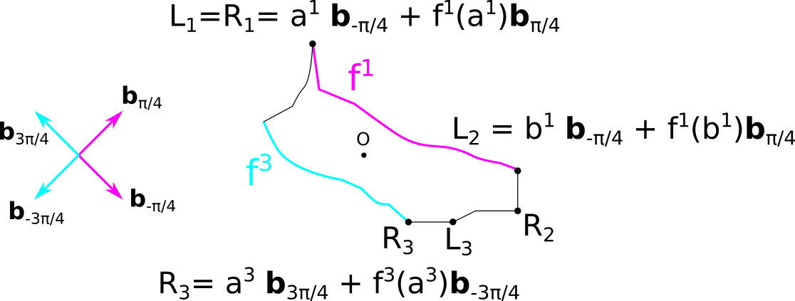
Figure 21: A curve in $\mathcal{E}$ and associated splitting in terms of the poles and the four regions $[R_{k},L_{k+1}]$ (with $L_{k+1}:=L_{1}$ if $k=4$) where the curve corresponds to the graph of a function $f^{k}$ in a reference frame with vectors $({\bf b}_{\pi/4-k\pi/2},{\bf b}_{\pi/4-(k-1)\pi/2})$ ($1\leq k\leq 4$). Region 1 is in magenta, regions 2 and 4 in black and region 3 in cyan. The coordinates of $L_{1}=R_{1}$ and $L_{2}$ are written in the the first reference frame $({\bf b}_{-\pi/4},{\bf b}_{\pi/4})$, and of $R_{3}$ in the third reference frame $({\bf b}_{3\pi/4},{\bf b}_{-3\pi/4})$.

$$\gamma=\bigcup_{k=1}^{4}P_{k}(\gamma)\cup\bigcup_{k=1}^{4}\Big{\{}u{\bf b}_{\pi/4-k\pi/2}+f^{k}(u){\bf b}_{\pi/4-(k-1)\pi/2}:u\in[a^{k},b^{k}]\Big{\}},$$ (B.41)

where the extremities $a^{k},b^{k}$ are chosen here to correspond to coordinates of $R_{k}(\gamma),L_{k+1}(\gamma)$ (with $L_{k+1}(\gamma):=L_{1}(\gamma)$ if $k=4$):

$$a^{k}=a^{k}(\gamma):=R_{k}(\gamma)\cdot{\bf b}_{\pi/4-k\pi/2},\quad b^{k}=b^{k}(\gamma):=L_{k+1}(\gamma)\cdot{\bf b}_{\pi/4-k\pi/2}.$$ (B.42)

For $1\leq k\leq 4$, let $u\in(a^{k},b^{k})$, and write $\gamma(u)$ for the corresponding point of $\gamma$:

$$\gamma(u):=u{\bf b}_{\pi/4-k\pi/2}+f^{k}(u){\bf b}_{\pi/4-(k-1)\pi/2}.$$ (B.43)

The derivative of $w\mapsto\gamma(w)$ at $u$, if it exists, is given by:

$$\frac{\sqrt{2}}{2}\Big{(}{\bf b}_{\pi/4-k\pi/2}+\partial_{u}f^{k}(u){\bf b}_{\pi/4-(k-1)\pi/2}\Big{)}={\bf t}(\gamma(u)),$$ (B.44)

where ${\bf t}$ is the $1$-normed tangent vector, defined in (3.85) in the first region. Recall that ${\bf T}:={\bf t}/\mathsf{v}$, where $\mathsf{v}:=\|{\bf t}\|_{2}$ and the arclength coordinate $s(u)$ satisfy:

$$ds(u)=\sqrt{1+(\partial_{u}f^{k}(u))^{2}}du=\sqrt{2}\mathsf{v}(\gamma(u))dx.$$ (B.45)

For each $t\in[0,T]$ and each curve $\gamma\in\mathcal{E}$, one can then write for $F_{H_{t},\varepsilon}$:

$$F_{H_{t},\varepsilon}(\gamma)=\frac{1}{2\sqrt{2}}\sum_{k=1}^{4}\int_{a^{k}+\varepsilon/\sqrt{2}}^{b^{k}-\varepsilon/\sqrt{2}}q^{k}_{H_{t},\varepsilon}(u,\gamma)du,$$ (B.46)

with, for $u\in(a^{k}+\varepsilon/\sqrt{2},b^{k}-\varepsilon/\sqrt{2})$:

$$q^{k}_{H_{t},\varepsilon}(u,\gamma):=\Big{(}(\mathsf{v}^{\varepsilon})^{2}\big{[}{\bf T}^{\varepsilon}\cdot{\bf m}\big{]} {\bf T}^{\varepsilon}\Big{)}\big{(}\gamma(u)\big{)}\cdot\nabla H_{t}\big{(}\gamma(u)\big{)}.$$ (B.47)

Recall from Definition 3.1 that ${\bf m}=(\pm 1,\pm 1)$ has a fixed value inside each region. Recall also the definitions of $v^{\varepsilon},{\bf T}^{\varepsilon}$ and their relationship with ${\bf t}^{\varepsilon}$ from (3.88)-(3.87): if $u\in(a^{1}+\varepsilon/\sqrt{2},b^{1}-\varepsilon/\sqrt{2})$ is in the first region for definiteness,

$${\bf t}^{\varepsilon}(\gamma(u))=\mathsf{v}^{\varepsilon}(\gamma(u)){\bf T}^{\varepsilon}(\gamma(u)) =\frac{1}{\sqrt{2}\varepsilon}\int_{u-\varepsilon/\sqrt{2}}^{u+\varepsilon/\sqrt{2}}{\bf t}(\gamma(w))dw$$

$$=\frac{\sqrt{2}}{2}\Big{(}{\bf b}_{-\pi/4}+\frac{f^{1}\big{(}u+\varepsilon/\sqrt{2}\big{)}-f^{1}\big{(}u-\varepsilon/\sqrt{2}\big{)}}{\varepsilon\sqrt{2}}{\bf b}_{\pi/4}\Big{)}.$$ (B.48)

For future reference, note that (B.48) implies the continuity of $q^{k}_{H_{t},\varepsilon}(u,\cdot)$ on $\mathcal{E}$ in Hausdorff distance for each $u\in(a^{k}+\varepsilon/\sqrt{2},b^{k}-\varepsilon/\sqrt{2})$, in the following sense: if $(\gamma^{n})_{n}\subset\mathcal{E},\gamma\in\mathcal{E}$ satisfy $\lim_{n}d_{\mathcal{H}}(\gamma^{n},\gamma)=0$ and if $u\in\big{(}a^{k}(\gamma)+\varepsilon/\sqrt{2},b^{k}(\gamma)-\varepsilon/\sqrt{2}\big{)}$, then $\lim_{n}q^{k}_{H_{t},\varepsilon}(u,\gamma^{n})=q^{k}_{H_{t},\varepsilon}(u,\gamma)$. Indeed, convergence in Hausdorff distance implies uniform convergence of $f^{k}$ around each such point $u$, and the expression (B.48) (or a similar one in region $k\neq 1$) yield the continuity.

We now apply the decomposition (B.46) to each $\gamma^{n}_{t}$, and use the control of the pole in (B.40) to express the integral on each region independently of $a^{k}(\gamma^{n}_{t}),b^{k}(\gamma^{n}_{t})$. Thanks to the indicator function in (B.46), one has for each $\zeta<\varepsilon/2$, each time $t$ and each $k$ with $1\leq k\leq 4$:

$$a^{k}(\gamma_{t})\leq a^{k}(\gamma^{n}_{t})+\frac{\zeta}{2}\leq a^{k}(\gamma^{n}_{t})+\frac{\varepsilon}{2\sqrt{2}},\qquad b^{k}(\gamma_{t})-\frac{\varepsilon}{2\sqrt{2}}\leq b^{k}(\gamma_{t})-\frac{\zeta}{2}\leq b^{k}(\gamma^{n}_{t}).$$ (B.49)

Since $q_{H_{t},\varepsilon}$ is bounded on $\mathcal{E}$:

$$\max_{1\leq k\leq 4}\sup_{t\leq T}\sup_{\gamma\in\mathcal{E}}\sup_{u\in(a^{k}+\varepsilon/\sqrt{2},b^{k}-\varepsilon/\sqrt{2}}|q_{H_{t},\varepsilon}(\gamma,u)|<\infty,$$ (B.50)

it is therefore enough to prove:

$$\limsup_{\zeta\rightarrow\infty}\lim_{n\rightarrow\infty}\int_{0}^{T}{\bf 1}\Big{\{}\max_{1\leq k\leq 4}\big{\{}\|L_{k}(\gamma^{n}_{t})-L_{k}(\gamma_{t})\|_{1}+\|R_{k}(\gamma^{n}_{t})-L_{k}(\gamma_{t})\|_{1}\big{\}}\leq\zeta\Big{\}}$$

$$\hskip 113.81102pt\times\sum_{k=1}^{4}\int_{a^{k}(\gamma_{t})+\varepsilon/\sqrt{2}}^{b^{k}(\gamma_{t})-\varepsilon/\sqrt{2}}\big{|}q^{k}_{H_{t},\varepsilon}(u,\gamma_{t}^{n})-q^{k}_{H_{t},\varepsilon}(u,\gamma_{t})\big{|}du=0.$$ (B.51)

At this point the dependence on the poles has been completely taken care of, and it will be enough to study $q^{k}_{H_{t},\varepsilon}$. Let $I_{\zeta}$ be the set of times in the first line above. To prove (B.51), we prove:

$$\lim_{n\rightarrow\infty}q^{k}_{H_{t},\varepsilon}(u,\gamma_{t}^{n})=q^{k}_{H_{t},\varepsilon}(u,\gamma_{t})\quad\text{for each }t\in I_{\zeta},\ u\in(a^{k}(\gamma_{t})+\varepsilon/\sqrt{2},b^{k}(\gamma_{t})-\varepsilon/\sqrt{2}).$$ (B.52)

Since $q^{k}_{H_{t},\varepsilon}$ is bounded on $\mathcal{E}$ for each $k$ by (B.50), (B.52) and the dominated convergence theorem yield (B.51).
To prove (B.52), notice that $\lim_{n}d_{E}(\gamma^{n}_{\cdot},\gamma_{\cdot})=0$ implies convergence in volume at almost every time: $\lim_{n}d_{L^{1}}(\gamma^{n}_{t},\gamma_{t})=0$ for almost every $t$. Now, by Lemma B.10, for each point $x$ at 1-distance at least $\lambda>0$ from the poles, convergence in volume of $\gamma^{n}_{t}\cap B_{1}(x,\lambda)$ implies convergence in Hausdorff distance. But we already saw below (B.48) that $q^{k}_{H_{t},\varepsilon}(u,\cdot)$ is continuous in Hausdorff distance for any $u$ corresponding to a point at 1-distance at least $\varepsilon$ from the poles. This implies (B.52) and concludes the proof of the continuity of (B.33).

To conclude the proof of Proposition 4.1, it remains to establish:

$$\forall\gamma_{\cdot}\in E([0,T],\mathcal{E}),\qquad\lim_{\varepsilon\rightarrow 0}J_{H,\varepsilon}^{\beta}(\gamma_{\cdot})=J_{H}^{\beta}(\gamma_{\cdot}).$$ (B.53)

Recalling Definition (2.47) of $J_{H}^{\beta}$, the above statement boils down to proving convergence of the terms in (B.33). As $\gamma_{\cdot}\in E([0,T],\mathcal{E})$ implies that $\int_{0}^{T}|\gamma_{t}|dt<\infty$, this is an immediate consequence of the expression (B.48) of the tangent vector, of the bound (B.50) and of the dominated convergence theorem. This concludes the proof of Proposition 4.1.

B.3 Exponential tightness

In this section, we use the characterisation of compact sets of Proposition B.8 to prove exponential tightness of the laws $\{\mathbb{P}^{N}_{\beta}:N\in\mathbb{N}^{*}\}$ inside $E([0,T],\mathcal{E})$ for each $T>0,\beta>1$. We first give a sufficient condition for exponential tightness, in Corollary B.12, then prove that it is satisfied in the rest of the section. The main difficulty lies, once again, in the control of the poles. To start with, the following characterisation of convergence in the volume distance $d_{L^{1}}$ will be useful.

Lemma B.11.

Let $(G_{\ell})_{\ell\geq 1}$ be a family of functions of $C^{2}_{c}(\mathbb{R}^{2},\mathbb{R})$, dense for the uniform norm $\sup_{\mathbb{R}^{2}}|\cdot|$ in the separable set $C_{c}(\mathbb{R}^{2},R)$. Then $d_{L^{1}}$ is topologically equivalent to the distance $\tilde{d}_{L^{1}}$ defined as follows: if $\gamma^{1},\gamma^{2}\in\Omega$ have associated droplet $\Gamma^{1},\Gamma^{2}$:

$$\tilde{d}_{L^{1}}(\Gamma^{1},\Gamma^{2})=\sum_{\ell\geq 1}\frac{1}{2^{\ell}}\frac{\big{|}\big{<}\Gamma^{1},G_{\ell}\big{>}-\big{<}\Gamma^{2},G_{\ell}\big{>}\big{|}}{1+\big{|}\big{<}\Gamma^{1},G_{\ell}\big{>}-\big{<}\Gamma^{2},G_{\ell}\big{>}\big{|}}.$$ (B.54)

In the sequel, $\tilde{d}_{L^{1}}$ and $d_{L^{1}}$ are identified.

To prove exponential tightness, we replace the condition on the Hausdorff distance, in Proposition B.8, by a condition on the positions of the extremities $L_{k},R_{k},1\leq k\leq 4$ of the poles. This condition, stated next, is more convenient to check at the microscopic level.

Corollary B.12 (Sufficient condition for tightness).

Let $T>0$. Assume that, for each $G\in C^{2}_{c}(\mathbb{R}^{2})$ and each $\varepsilon>0$,

$$\limsup_{\eta\rightarrow 0}\limsup_{N\rightarrow\infty}\frac{1}{N}\log\mathbb{P}^{N}_{\beta}\bigg{(}\gamma^{N}_{\cdot}\in E([0,T],\mathcal{E})\cap\bigg{\{}\gamma_{\cdot}:\sup_{|s-t|\leq\eta}\big{|}\big{<}\Gamma_{t},G\big{>}-\big{<}\Gamma_{s},G\big{>}\big{|}$$ (B.55)

$$\hskip 91.04872pt+\sup_{h\leq\eta}\sum_{k=1}^{4}\int_{0}^{T-h}\|L_{k}(\gamma_{t})-L_{k}(\gamma_{t+h})\|_{1}dt\geq\varepsilon\bigg{\}}\bigg{)}=-\infty.$$

Then for each $H\in\mathcal{C}$ and $q\in\mathbb{N}^{*}$, there are compact sets $K_{q}=K_{q}(H)\subset E([0,T],\Omega)$ such that:

$$\sup_{N}\frac{1}{N}\log\mathbb{P}^{N}_{\beta,H}\big{(}\gamma^{N}_{\cdot}\in E([0,T],\mathcal{E})\cap(K_{q})^{c}\big{)}\leq-q.$$ (B.56)

Proof.

As (B.55) also holds under $\mathbb{P}^{N}_{\beta,H}$ for any $H\in\mathcal{C}$, we prove the corollary only for $H\equiv 0$.
Consider a sequence $G_{\ell}\in C^{2}_{c}(\mathbb{R}^{2}),\ell\geq 1$, dense for the uniform norm. According to (B.55), for each $q,n,\ell\in\mathbb{N}^{*}$, there is $\eta=\eta(q,\ell,n)$ and $N_{0}=N_{0}(\eta)$ such that:

$$\sup_{N\geq N_{0}} \frac{1}{N}\log\mathbb{P}^{N}_{\beta}\bigg{(}\gamma^{N}_{\cdot}\in E([0,T],\mathcal{E})\cap\bigg{\{}\sup_{|s-t|\leq\eta}\big{|}\big{<}\Gamma_{t},G_{\ell}\big{>}-\big{<}\Gamma_{s},G_{\ell}\big{>}\big{|}$$ (B.57)

$$\hskip 34.14322pt+\sup_{h\leq\eta}\sum_{k=1}^{4}\int_{0}^{T-h}\|L_{k}(\gamma_{t})-L_{k}(\gamma_{t+h})\|_{1}dt\geq\frac{1}{n}\bigg{\}}\cap\Big{\{}\sup_{t\leq T}|\gamma_{t}|\leq\frac{q\ell n}{C(\beta)}\Big{\}}\bigg{)}\leq-qn\ell.$$

For $N\leq N_{0}$, each of $\big{<}\Gamma^{N}_{\cdot},G\big{>}$ $L_{k}(\gamma^{N}_{\cdot})$ and $R_{k}(\gamma^{N}_{\cdot})$ for $k$ with $1\leq k\leq 4$ is a càdlàg function when $\gamma^{N}_{\cdot}$ is a trajectory in the space of $\Omega^{N}_{\text{mic}}\cap\mathcal{E}\cap\{|\gamma|\leq qn\ell/C(\beta)\}$-valued trajectories that are càdlàg in Hausdorff distance. This set is complete and separable, as $\Omega^{N}_{\text{mic}}\cap\mathcal{E}\cap\{|\gamma|\leq qn\ell/C(\beta)\}$ is compact by Proposition B.2. As a result, (B.57) holds for $N\leq N_{0}$ as well up to choosing $\eta^{\prime}=\eta^{\prime}(q,\ell,n)\leq\eta$, hence for all $N$ in $\mathbb{N}^{*}$. For $G\in C^{2}_{c}(\mathbb{R}^{2})$, let thus $m_{\cdot}^{L^{1}}\big{(}\big{<}\Gamma_{\cdot},G\big{>}\big{)}$ be the Skorokhod modulus of continuity associated with the trajectory $\big{(}\big{<}\Gamma_{t},G\big{>}\big{)}_{t}$. It satisfies:

$$\forall\theta>0,\qquad m_{\theta}^{L^{1}}\big{(}\big{<}\Gamma_{\cdot},G\big{>}\big{)}\leq\sup_{|s-t|\leq\theta}\big{|}\big{<}\Gamma_{t},G\big{>}-\big{<}\Gamma_{s},G\big{>}\big{|}.$$ (B.58)

Recall the control on the length obtained in Lemma 6.1, in particular the definition of $C(\beta)>0$. Define then $K_{q}=\bar{U}_{q}$, with $U_{q}$ as follows:

$$U_{q} :=\Big{\{}\sup_{t\leq T}|\gamma_{t}|\leq\frac{q}{C(\beta)}\Big{\}}$$

$$\qquad\cap\bigcap_{\ell,n\in\mathbb{N}^{*}}\bigg{\{}m_{\eta^{\prime}}^{L^{1}}\big{(}\big{<}\Gamma_{\cdot},G_{\ell}\big{>}\big{)}+\sup_{h\leq\eta^{\prime}} \sum_{k=1}^{4}\int_{0}^{T-h}\|L_{k}(\gamma_{t})-L_{k}(\gamma_{t+h})\|_{1}dt\leq\frac{1}{n}\bigg{\}}.$$ (B.59)

By Proposition B.8 and Lemma B.4, $K_{q}$ is compact. Moreover, it satisfies by construction:

$$\sup_{N\in\mathbb{N}^{*}}\frac{1}{N}\log\mathbb{P}^{N}_{\beta}\big{(}\gamma^{N}_{\cdot}\in E([0,T],\mathcal{E})\cap(K_{q})^{c}\big{)}\leq-q.$$ (B.60)

This concludes the proof of exponential tightness inside $E([0,T],\mathcal{E})$. ∎

We conclude the section by a proof of relative compactness of the laws of the dynamics for short time.

Corollary B.13.

Let $\beta>1$, $H\in\mathcal{C}$ and $(\mu^{N})_{N}$ be a sequence of probability measures on $\big{(}\mathcal{E},d_{L^{1}}\big{)}$ converging weakly to $\delta_{\gamma^{\text{ref}}}$. Assume further that there is $t_{0}>0$ such that:

$$\lim_{N\rightarrow\infty}\mathbb{P}^{\mu^{N}}_{\beta,H}(\gamma^{N}_{\cdot}\in E([0,t_{0}],\mathcal{E}))=1.$$ (B.61)

Still write $d_{E}$ for the distance (B.13) defined on a time interval $[0,t_{0}]$. Then the set $\{\mathbb{P}^{\mu^{N}}_{\beta,H}:N\in\mathbb{N}^{*}\}$ is relatively compact in the set of probability measures on $\big{(}E([0,t_{0}],\Omega),d_{E}\big{)}$, and its limit points are supported on trajectories in $E([0,t_{0}],\mathcal{E})$ that are continuous in $d_{L^{1}}$ distance.

Proof.

By the direct half of Prokhorov theorem (Theorem 5.1 in [Bil99]), relative compactness is implied by tightness. Let us therefore prove that $\{\mathbb{P}^{N}_{\beta,H}\}_{N}$ is tight in $E([0,t_{0}],\Omega)$. The proof is a bit indirect because Corollary B.12 only gives a good control of trajectories in $E([0,t_{0}],\mathcal{E})$, not in $E([0,t_{0}],\Omega)$. For each measurable set $B\subset E([0,t_{0}],\Omega)$, write:

$$\mathbb{P}^{\mu^{N}}_{\beta,H}(\gamma^{N}_{\cdot}\in B) =\mathbb{P}^{\mu^{N}}_{\beta,H}\big{(}\gamma^{N}_{\cdot}\in B\cap E([0,t_{0}],\mathcal{E})\big{)}+\mathbb{P}^{\mu^{N}}_{\beta,H}\big{(}\gamma^{N}_{\cdot}\in B\cap E([0,t_{0}],\mathcal{E})^{c}\big{)}.$$ (B.62)

Fix $\eta>0$. By Assumption (B.61), there is $N_{0}(\eta)\in\mathbb{N}^{*}$ such that:

$$\mathbb{P}^{\mu^{N}}_{\beta,H}\big{(}\gamma^{N}_{\cdot}\in E([0,t_{0}],\mathcal{E})^{c}\big{)}\leq\eta.$$ (B.63)

On the other hand, the initial conditions $(\mu^{N})_{N}$ are probability measures on $\mathcal{E}$, which is separable and complete for $d_{L^{1}}$ (seeing $\mathcal{E}$ as a closed subset of $L^{1}(\mathbb{R}^{2})$ by identifying curves with the indicator functions of their associated droplets). It follows from the converse half of Prokhorov’s theorem (Theorem 5.2 in [Bil99]) that $(\mu^{N})_{N}$ is tight. For each $\eta>0$, let thus $K^{0}_{\eta}\subset\mathcal{E}$ be a compact set for the distance $d_{L^{1}}$, such that:

$$\forall N\in\mathbb{N}^{*},\qquad\mathbb{P}^{\mu^{N}}_{\beta,H}\Big{(}\gamma^{N}_{0}\in\big{(}K^{0}_{\eta}\big{)}^{c}\Big{)}=\mu^{N}\Big{(}\gamma^{N}\in\big{(}K^{0}_{\eta}\big{)}^{c}\Big{)}\leq\eta.$$ (B.64)

Then, for each $q\in\mathbb{N}^{*}$ with $e^{-q}\leq\eta$, recalling the definition of $K_{q}$ from Corollary B.12:

$$\forall N\in\mathbb{N}^{*},\qquad\mathbb{P}^{\mu^{N}}_{\beta,H}\Big{(}\gamma^{N}_{\cdot}\in E([0,t_{0}],\mathcal{E})\cap\big{(}K^{0}_{\eta}\cap K_{q}\big{)}^{c}\Big{)}\leq 2\eta.$$ (B.65)

As a result, for $N\geq N_{0}(\eta)$, we have:

$$\mathbb{P}^{\mu^{N}}_{\beta,H}\Big{(}\gamma^{N}_{\cdot}\in\big{(}K^{0}_{\eta}\cap K_{q}\big{)}^{c}\Big{)}\leq 3\eta.$$ (B.66)

Now, each $\mathbb{P}^{\mu^{N}}_{\beta,H}$ for $N<N_{0}(\eta)$ is a probability measure on the complete, separable set $D_{\mathcal{H}}([0,t_{0}],\Omega)$ of càdlàg trajectories in Hausdorff distance with values in $\Omega$. In particular, for each $N<N_{0}(\eta)$, $\mathbb{P}^{\mu^{N}}_{\beta,H}$ is tight. There is thus a compact set $K^{N}_{\eta}\subset D_{\mathcal{H}}([0,t_{0}],\Omega)$ such that:

$$\mathbb{P}^{\mu^{N}}_{\beta,H}\Big{(}\gamma^{N}_{\cdot}\in\big{(}K^{N}_{\eta}\big{)}^{c}\Big{)}\leq\eta,\qquad N<N_{0}(\eta).$$ (B.67)

Since convergence in $D_{\mathcal{H}}([0,t_{0}],\Omega)$ implies convergence for $d_{E}$, each $K^{N}_{\eta}$ is also a compact set for $d_{E}$, whence the proof of tightness in $E([0,t_{0}],\Omega)$:

$$\forall N\in\mathbb{N}^{*},\qquad\mathbb{P}^{\mu^{N}}_{\beta,H}\Big{(}\gamma^{N}_{\cdot}\in\bigcap_{M<N_{0}(\eta)}\big{(}K^{M}_{\eta}\big{)}^{c}\cap\big{(}K^{0}_{\eta}\cap K_{q}\big{)}^{c}\Big{)}\leq 3\eta.$$ (B.68)

It remains to check that $\{\mathbb{P}^{\mu^{N}}_{\beta,H}:N\in\mathbb{N}^{*}\}$ concentrates on trajectories that are continuous in volume, $d_{L^{1}}$ distance. This is a standard consequence of the estimate (B.55), so we conclude the proof here. ∎

B.3.1 Estimate in $L^{1}(\mathbb{R}^{2})$ topology

In this section, we prove exponential tightness in volume, i.e. in $L^{1}(\mathbb{R}^{2})$.

Lemma B.14.

Let $\beta>1$, $T>0$ and $G\in C^{2}_{c}(\mathbb{R}^{2})$. Then, for each $\varepsilon>0$:

$$\limsup_{\eta\rightarrow 0}\limsup_{N\rightarrow\infty}\frac{1}{N}\log\mathbb{P}^{N}_{\beta}\Big{(}\gamma^{N}_{\cdot}\in E([0,T],\mathcal{E})\cap\Big{\{}\sup_{|t-s|\leq\eta}\big{|}\big{<}\Gamma^{N}_{t},G\big{>}-\big{<}\Gamma^{N}_{s},G\big{>}\big{|}>\varepsilon\Big{\}}\Big{)}=-\infty.$$

The result also holds under $\mathbb{P}^{N}_{\beta,H}$ for $H\in\mathcal{C}$ by Corollary 6.2.

Proof.

Compared to Chapter 10 in [KL99], the only subtleties to prove Lemma B.14 are in the introduction of the condition $E([0,T],\mathcal{E})$, and in the control of the change in volume induced by the motion of the poles. As these do not present any particular difficulty, the proof is omitted. ∎

B.3.2 Precise control of the slope and volume around the poles

As preliminary to proving the estimate of the behaviour of the poles in (B.55) we prove, in this section, that the volume beneath each pole is fixed by the reservoir-like behaviour induced by the dynamics. This will be used in Section B.3.3 to argue that a displacement of the poles must result in a change in volume, which is unlikely for short time by Lemma B.14.
The estimate of the volume beneath a pole relies on the microscopic estimate of the slope at the pole, obtained in Corollary 6.13. All stated results are valid under $\mathbb{P}^{N}_{\beta,H}$ for $H\in\mathcal{C}$ by Corollary 6.2.

Lemma B.15 (Control of the deviations of the width at distance $\alpha>0$ below the pole).

Let $\beta>1$. For $\alpha>0$ and $\gamma\in\mathcal{E}$, let $g^{+}(\alpha)=g^{+}(\alpha)(\gamma)$ be the width of the horizontal segment of $\gamma$ at height $z_{1}(\gamma)-\alpha$ to the right of $L_{1}(\gamma)$ (see Figure 22). Define similarly $g^{-}(\alpha)$ to the left of $L_{1}(\gamma)$. For each $\delta,\eta>0$:

$$\limsup_{\alpha\rightarrow 0}\limsup_{N\rightarrow\infty}\frac{1}{N}\log\mathbb{P}^{N}_{\beta}\bigg{(}\gamma^{N}_{\cdot}\in E([0,T],\mathcal{E})\cap\Big{\{}\frac{1}{T}\int_{0}^{T}{\bf 1}_{|\alpha^{-1}g^{\pm}(\alpha)-(e^{\beta}-1)|\geq\delta}dt>\eta\Big{\}}\bigg{)}=-\infty.$$

Proof.

The proof is a formalisation of Figure 22: since the slope on both sides of the pole is fixed by Corollary 6.13, we can obtain upper and lower bounds on $g^{\pm}$ in terms of $\beta$.
Take $\zeta^{1},\zeta^{2}>0$ to be determined later, and $\theta>0$ which will be small. The proof of the result is similar for $g^{+}$ and $g^{-}$, so we focus on $g^{+}$. It is sufficient to prove:

$$\limsup_{\zeta^{1},\zeta^{2}\rightarrow 0}\limsup_{\alpha\rightarrow 0}\limsup_{N\rightarrow\infty}\frac{1}{N}\log\mathbb{P}^{N}_{\beta}\bigg{(}\gamma_{\cdot}^{N}\in E([0,T],\mathcal{E});$$ (B.69)

$$\hskip 85.35826pt\frac{1}{T}\int_{0}^{T}{\bf 1}_{|\alpha^{-1}g^{+}(\alpha)-(e^{\beta}-1)|\geq\delta}{\bf 1}_{|\xi^{+,\zeta^{1}N}_{L_{1}}-e^{-\beta}|\leq\theta}{\bf 1}_{|\xi^{+,\zeta^{2}N}_{L_{1}}-e^{-\beta}|\leq\theta}dt>\eta/3\bigg{)}=-\infty.$$

Consider the event bearing on $\xi^{+,\zeta^{1}N}_{L_{1}}$. It enforces:

$$\xi^{+,\zeta^{1}N}_{L_{1}}\in[e^{-\beta}-\theta,e^{-\beta}+\theta].$$ (B.70)

Figure 22: Neighbourhood of the north pole of a microscopic curve for which $g^{+}(\alpha)$ is drawn (horizontal magenta arrow). On the left figure, black dots delimit the $\zeta^{1}N$ edges to the right of $L_{1}$, with $\zeta^{1}$ chosen to ensure $\zeta^{1}\xi^{+,\zeta^{1}N}\geq\alpha$ (this quantity represented by cyan arrows). On the right figure, $\zeta^{2}$ is similarly chosen so that $\zeta^{2}\xi^{+,\zeta^{2}N}\leq\alpha$ (in cyan arrows again). Since bounds on $\zeta^{1}\xi^{+,\zeta^{1}N},\zeta^{2}\xi^{+,\zeta^{2}N}$ are available in terms of $\beta$, $g^{+}(\alpha)$ can be bounded.

Choose $\zeta^{1}$ such that $(e^{-\beta}-\theta)\zeta^{1}=\alpha$. Then $\zeta^{1}\xi^{+,\zeta^{1}N}_{L_{1}}\geq\alpha$ (see Figure 22). By definition, $g^{+}(\alpha)$ must thus be smaller than $\zeta^{1}(1-\xi^{+,\zeta^{1}N}_{L_{1}})$:

$$\xi^{+,\zeta^{1}N}_{L_{1}} \in[e^{-\beta}-\theta,e^{-\beta}+\theta]\text{ and }(e^{-\beta}-\theta)\zeta^{1}=\alpha$$

$$\quad\Rightarrow\quad\alpha^{-1}g^{+}(\alpha)\leq\frac{1-e^{-\beta}+\theta}{e^{-\beta}-\theta}=e^{\beta}-1+O(\theta),$$ (B.71)

where $O(\theta)$ is a positive function. Similarly, choose $\zeta^{2}$ such that $(e^{-\beta}+\theta)\zeta^{2}=\alpha$. Then $g^{+}(\alpha)\geq\zeta^{2}(1-\xi^{+,\zeta^{2}N}_{L_{1}})$, thus:

$$\xi^{+,\zeta^{2}N}_{L_{1}} \in[e^{-\beta}-\theta,e^{-\beta}+\theta]\text{ and }(e^{-\beta}+\theta)\zeta^{2}=\alpha$$

$$\quad\Rightarrow\quad\alpha^{-1}g^{+}(\alpha)\geq\frac{1-e^{-\beta}-\theta}{e^{-\beta}+\theta}=e^{\beta}-1-O(\theta).$$ (B.72)

$O(\theta)$ is again a positive function. Taking $\theta$ small enough to contradict $|\alpha^{-1}g^{+}(\alpha)-(e^{\beta}-1)|\geq\delta$ concludes the proof. ∎

Lemma B.16 (Control of the deviations of the volume at distance $\alpha>0$ below the pole).

For $\gamma\in\mathcal{E}$ with associated droplet $\Gamma$, let $V^{\alpha}=V^{\alpha}(\gamma)$ be defined as:

$$V^{\alpha}(\gamma)=\alpha^{-2}\big{|}\{x\in\Gamma:x\cdot{\bf b}_{2}\geq z_{1}(\gamma)-\alpha\}\big{|}.$$ (B.73)

Then for each $\beta>1$ and each $\delta,\eta>0$:

$$\limsup_{\alpha\rightarrow 0}\limsup_{N\rightarrow\infty}\frac{1}{N}\log\mathbb{P}^{N}_{\beta}\bigg{(}\gamma^{N}_{\cdot}\in E([0,T],\mathcal{E})\cap\Big{\{}\frac{1}{T}\int_{0}^{T}{\bf 1}_{|V^{\alpha}-(e^{\beta}-1)|>\delta}dt>\eta\Big{\}}\bigg{)}=-\infty.$$ (B.74)

Proof.

The idea is to use Lemma B.15 at multiple depths to prove that a droplet beneath the pole must be approximately triangular. Fix $\ell\in\mathbb{N}^{*}$ and $\theta>0$ to be chosen later. By Lemma B.15, it is sufficient to prove:

$$\limsup_{\alpha\rightarrow 0}\limsup_{N\rightarrow\infty}\frac{1}{N}\log\mathbb{P}^{N}_{\beta}\bigg{(} \gamma^{N}_{\cdot}\in E([0,T],\mathcal{E});$$ (B.75)

$$\frac{1}{T}\int_{0}^{T}{\bf 1}_{|V^{\alpha}-(e^{\beta}-1)|>\delta}{\bf 1}_{\forall j\in\{1,...,\ell\},\big{|}\frac{\ell}{j\alpha}g^{\pm}(j\alpha/\ell)-(e^{\beta}-1)\big{|}\leq\theta}dt>\eta/2\bigg{)}=-\infty.$$

By definition of $g^{\pm}(\alpha)=g^{\pm}(\alpha)(\gamma)$ for $\alpha>0$ and $\gamma\in\mathcal{E}$ (see Lemma B.15), the quantity $V^{\alpha}(\gamma)$ satisfies:

$$V^{\alpha}(\gamma)=\alpha^{-2}\int_{0}^{\alpha}(g^{+}(u)+g^{-}(u))du.$$ (B.76)

As elements of $\Omega$ have $1$-Lipschitz boundaries, if a curve $\gamma\in\Omega$ is such that $(\ell/j\alpha)g^{\pm}(j\alpha/\ell)\in[e^{\beta}+1-\theta,e^{\beta}-1-\theta]$ for each $1\leq j\leq\ell$, then:

$$\alpha^{2}V^{\alpha}(\gamma)=|\{x\in\Gamma:x\cdot{\bf b}_{2}\geq z_{1}-\alpha\}|\geq 2\sum_{j=1}^{\ell-1}\frac{j}{\ell\alpha}(e^{\beta}+1-\theta)\times\frac{\alpha}{\ell}=\frac{\ell-1}{\ell}(e^{\beta}-1-\theta)\alpha^{2}.$$ (B.77)

Similarly,

$$\alpha^{2}V^{\alpha}(\gamma)\leq 2\sum_{j=1}^{\ell}\frac{j}{\ell\alpha}(e^{\beta}+1-\theta)\times\frac{\alpha}{\ell}=\frac{\ell+1}{\ell}(e^{\beta}-1+\theta)\alpha^{2}.$$ (B.78)

To conclude the proof, it remains to take $\ell,\theta$ such that the indicator functions appearing in (B.75) bear on incompatible events. This is achieved provided:

$$\frac{\ell-1}{\ell}(e^{\beta}-1-\theta)\geq e^{\beta}-1-\delta\quad\text{and}\quad\frac{\ell+1}{\ell}(e^{\beta}-1+\theta)\leq e^{\beta}-1+\delta.$$ (B.79)

∎

B.3.3 Tightness in $L^{1}([0,T])$ distance for the motion of the poles

In this section, we conclude the proof of (B.55) by providing the estimate on the motion of the poles, more precisely on the components $w_{k},z_{k}$ of the $L_{k}$, $1\leq k\leq 4$. We prove the result for $z_{1}$, the other seven coordinates being similar (see Remark B.18 below).

Lemma B.17 (Tightness in $L^{1}$ distance for $z_{1}$).

Let $\beta>1$ and $A,\varepsilon>0$. Then:

$$\limsup_{\eta\rightarrow 0}\limsup_{N\rightarrow\infty}\frac{1}{N}\log\mathbb{P}^{N}_{\beta}\bigg{(}\gamma^{N}_{\cdot} \in E([0,T],\mathcal{E})\cap\Big{\{}\ \sup_{t\leq T}|\gamma^{N}_{t}|\leq A\Big{\}}$$ (B.80)

$$\quad\cap\Big{\{}\sup_{h\leq\eta}\frac{1}{T}\int_{0}^{T-h}|z_{1}(\gamma^{N}_{t+h})-z_{1}(\gamma^{N}_{t})|dt>\varepsilon\Big{\}}\bigg{)}=-\infty.$$

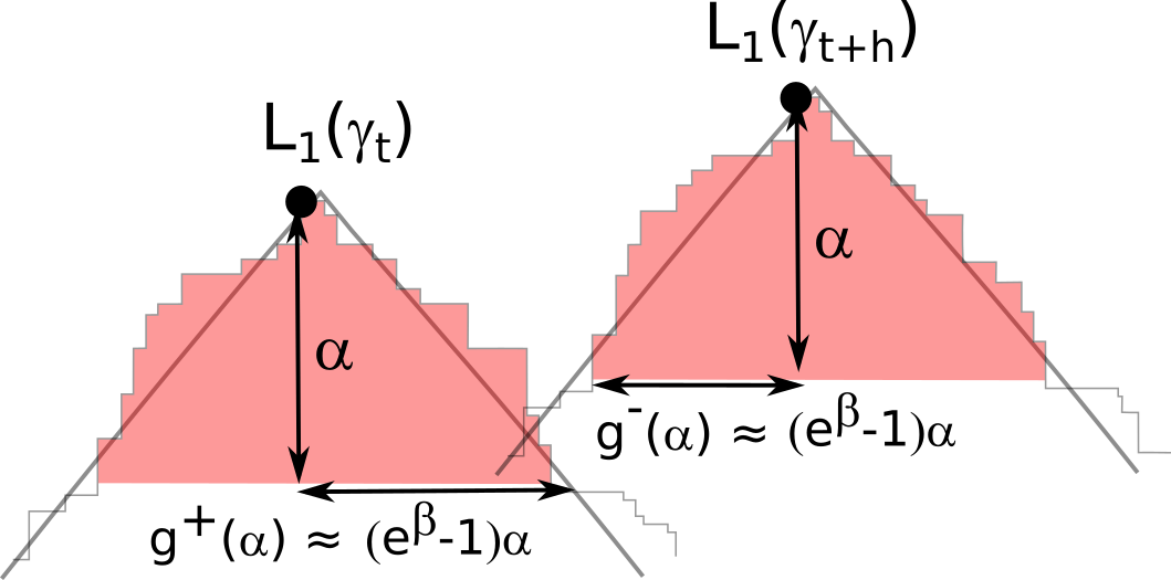
Figure 23: Neighbourhood of the north pole of a microscopic curve at times $t$, $t+h$. Under the contour dynamics, sufficiently close to the poles (corresponding to the parameter $\alpha\ll 1$ on the figure), the poles stand atop a triangular shape (red shaded area) with a slope fixed in terms of $\beta$. Equivalently, the width $g^{\pm}(\alpha)$ is approximately given by $\alpha(e^{\beta}-1)$. A displacement of the poles leads to a shift of the triangle and thus implies a change in volume, i.e. for the distance $d_{L^{1}}$.

Proof.

Let $\gamma_{\cdot}\in E([0,T],\mathcal{E})$. The idea is the following. Results of Section B.3.2 imply that the pole dynamics creates triangular shapes in the curves, with a slope fixed in terms of $\beta$ (see Figure 23). Moving a pole thus means moving one of these triangles, which has a volume. In that way motion of the poles is linked with a displacement of the volume, which we know cannot happen instantaneously by Lemma B.14.

For each $h\leq\eta$ and each $t\in[0,T-h]$, write $\Delta_{h}(t)$ for the difference $|z_{1}(\gamma_{t+h})-z_{1}(\gamma_{t})|$ for brevity. By Definition 2.5 of the initial condition and owing to the bound on the length, $z_{1}(\gamma_{\cdot})$ is bounded by $A+C_{0}$ for some $C_{0}=C_{0}(\gamma^{\text{ref}})>0$ on the event in (B.80). Equation (B.80) is thus proven as soon as:

$$\limsup_{\eta\rightarrow 0}\limsup_{N\rightarrow\infty}$$ (B.81)

$$\quad\frac{1}{N}\log\mathbb{P}^{N}_{\beta}\bigg{(}\gamma^{N}_{\cdot}\in E([0,T],\mathcal{E})\cap\Big{\{}\sup_{h\leq\eta}\frac{1}{T}\int_{0}^{T-h}{\bf 1}_{\Delta_{h}(t)\geq\varepsilon/2}dt>\frac{\varepsilon}{2(A+C_{0})}\Big{\}}\bigg{)}=-\infty.$$

Fix $\delta>0$ that will be chosen small enough in the following. Recall that, for $\alpha>0$, $V^{\alpha}$ is the volume below the pole times $\alpha^{-2}$, see Lemma B.16. For $\alpha>0$ and $t\in[0,T]$, define then $\Delta V^{\alpha}(t)$ as follows :

$$\Delta V^{\alpha}(t)=|V^{\alpha}(\gamma_{t})-(e^{\beta}-1)|.$$ (B.82)

Lemma B.16 tells us:

$$\limsup_{\alpha\rightarrow 0}\limsup_{N\rightarrow\infty}\frac{1}{N}\log\mathbb{P}^{N}_{\beta}\bigg{(}\gamma^{N}_{\cdot}\in E([0,T],\mathcal{E})\cap\Big{\{}\frac{1}{T}\int_{0}^{T}{\bf 1}_{\Delta V^{\alpha}(t)>\delta}dt>\frac{\varepsilon}{6(A+C_{0})}\Big{\}}\bigg{)}=-\infty.$$ (B.83)

Notice in addition that:

$$\Big{\{}\sup_{h\leq\eta}\frac{1}{T}\int_{0}^{T-h}{\bf 1}_{\Delta V^{\alpha}(t+h)>\delta}dt>\frac{\varepsilon}{6(A+C_{0})}\Big{\}}\subset\Big{\{}\frac{1}{T}\int_{0}^{T}{\bf 1}_{\Delta V^{\alpha}(t)>\delta}dt>\frac{\varepsilon}{6(A+C_{0})}\Big{\}}.$$ (B.84)

As a result, if $\lambda$ denotes $T^{-1}$ times the Lebesgue measure on $[0,T]$, (B.80) holds as soon as:

$$\limsup_{\alpha\rightarrow 0}\limsup_{\eta\rightarrow 0}\limsup_{N\rightarrow\infty}\frac{1}{N}\log\mathbb{P}^{N}_{\beta}\bigg{(}\gamma^{N}_{\cdot}\in E([0,T],\mathcal{E});$$ (B.85)

$$\hskip 85.35826pt\sup_{h\leq\eta}\lambda\Big{[}\Delta_{h}(t)\geq\varepsilon/2,|\Delta V^{\alpha}(t)|\leq\delta,|\Delta V^{\alpha}(t+h)|\leq\delta\Big{]}>\frac{\varepsilon}{6(A+C_{0})}\bigg{)}=-\infty.$$

By Lemma B.14 on exponential tightness in $d^{S}_{L^{1}}$ topology, (B.85) is proven as soon as the following holds:

$$\limsup_{\alpha\rightarrow 0}\limsup_{\eta\rightarrow 0}\limsup_{N\rightarrow\infty}\frac{1}{N}\log\mathbb{P}^{N}_{\beta}\bigg{(}\gamma^{N}_{\cdot}\in E([0,T],\mathcal{E});\ \sup_{t\leq T}|\gamma^{N}_{t}|\leq A;$$

$$\hskip 85.35826pt\sup_{\begin{subarray}{c}(s,t)\in[0,T]^{2}\\ |s-t|\leq\eta\end{subarray}}d_{L^{1}}(\gamma^{N}_{s},\gamma^{N}_{t})<\frac{\alpha^{2}(e^{\beta}-1)}{2};$$ (B.86)

$$\hskip 85.35826pt\sup_{h\leq\eta}\lambda\Big{[}\Delta_{h}(t)\geq\varepsilon/2,|\Delta V^{\alpha}(t)|\leq\delta,|\Delta V^{\alpha}(t+h)|\leq\delta\Big{]}>\frac{\varepsilon}{6(A+C_{0})}\bigg{)}=-\infty.$$

Take $\delta<(e^{\beta}-1)/2$ and an arbitrary $\alpha\in(0,\varepsilon/2]$. Let us prove that the event in the probability in (B.86) is empty. For any trajectory $(\gamma^{N}_{t})_{t\in[0,T]}$ in this event, there must be $t\in[0,T]$ and $h<\eta$ such that, simultaneously:

• The north poles of $\Gamma^{N}_{t},\Gamma^{N}_{t+h}$ are at vertical distance at least $\varepsilon/2$, so that either $\{x\in\Gamma^{N}_{t}:x\cdot{\bf b}_{2}\geq z_{1}(\gamma^{N}_{t})-\alpha\}\cap\Gamma^{N}_{t+h}=\emptyset$ or $\{x\in\Gamma^{N}_{t+h}:x\cdot{\bf b}_{2}\geq z_{1}(\gamma^{N}_{t+h})-\alpha\}\cap\Gamma^{N}_{t}=\emptyset$.

• Recall that $V^{\alpha}(t)=\alpha^{-2}|\{x\in\Gamma^{N}_{t}:x\cdot{\bf b}_{2}\geq z_{1}(\gamma^{N}_{t})-\alpha\}|$. $V^{\alpha}(t)$ and $V^{\alpha}(t+h)$ are both bounded below by $e^{\beta}-1-\delta>(e^{\beta}-1)/2$ so that, by the first point, the difference in volume between $\Gamma^{N}_{t}$ and $\Gamma_{t+h}$ is at least $\alpha^{2}(e^{\beta}-1)/2$;

• yet, $d_{L^{1}}(\gamma^{N}_{t},\gamma^{N}_{t+h})<\alpha^{2}(e^{\beta}-1)/2$, which is incompatible with point 2. This concludes the proof.

∎

Remark B.18.

The proof for $z_{k}$ ($2\leq k\leq 4$) is identical to the above. For the $w_{k}$, i.e. $L_{1}\cdot{\bf b}_{1},L_{2}\cdot{\bf b}_{2},L_{3}\cdot{\bf b}_{1}$ and $L_{4}\cdot{\bf b}_{2}$, slight modifications are required: in addition to the indicator functions on the volumes $\Delta V^{\alpha}(t)<\delta$, $\Delta V^{\alpha}(t+h)<\delta$, one has to introduce the events $\{|\alpha^{-1}g^{\pm}_{\alpha}(t)-(e^{\beta}-1)|<\delta\},\{|\alpha^{-1}g^{\pm}_{\alpha}(t+h)-(e^{\beta}-1)|<\delta\}$, where $g^{\pm}_{\alpha}$, the width of the level at distance $\alpha$ beneath the pole, is defined in Lemma B.15.

The idea is then that, e.g. for $w_{1}$, if $\alpha$ is taken small enough as a function of $\varepsilon$ and $\beta$ ($(e^{\beta}-1)^{-1}\varepsilon/6$ works), then $|w_{1}(\gamma^{N}_{t})-w_{1}(\gamma^{N}_{t+h})|\geq\varepsilon/2$ implies that this difference must be larger than $\min\{g_{\alpha}^{+}(t+h)+g_{\alpha}^{-}(t),g_{\alpha}^{+}(t)+g_{\alpha}^{-}(t+h)\}$ (see Figure 23).

But then this means that the set of points above $z_{1}(\gamma^{N}_{t})-\alpha$ in $\Gamma^{N}_{t}$ and the set of points above $z_{1}(\gamma^{N}_{t+h})-\alpha$ in $\Gamma^{N}_{t+h}$ are disjoint. Thanks to the indicator functions on the volumes $\Delta V^{\alpha}$, this implies a difference in volume, which is again impossible for $\eta$ small enough.  $\blacksquare$

References

- [Lif62] I.M. Lifshitz “Kinetics of Ordering during Second-Order Phase Transitions” In Soviet Physics–JETP [translation of Zhurnal Eksperimentalnoi i Teoreticheskoi Fiziki] 15, 1962, pp. 939
- [DFL86] Anna De Masi, Pablo Augusto Ferrari and Joel L Lebowitz “Reaction-Diffusion Equations for Interacting Particle Systems” In Journal of statistical physics 44.3-4 Springer, 1986, pp. 589–644
- [Com87] Francis Comets “Nucleation for a Long Range Magnetic Model” In Annales de l’IHP Probabilités et Statistiques 23.2, 1987, pp. 135–178
- [GPV88] M.. Guo, G.. Papanicolaou and S… Varadhan “Nonlinear Diffusion Limit for a System with Nearest Neighbor Interactions” In Communications in Mathematical Physics 118.1 Springer, 1988, pp. 31–59 URL: https://projecteuclid.org/journals/communications-in-mathematical-physics/volume-118/issue-1/Nonlinear-diffusion-limit-for-a-system-with-nearest-neighbor-interactions/cmp/1104161907.full
- [KOV89] C. Kipnis, S. Olla and S.R.S. Varadhan “Hydrodynamics and Large Deviation for Simple Exclusion Processes” In Communications on Pure and Applied Mathematics 42.2 Wiley Online Library, 1989, pp. 115–137
- [ELS90] Gregory Eyink, Joel L Lebowitz and Herbert Spohn “Hydrodynamics of Stationary Non-Equilibrium States for Some Stochastic Lattice Gas Models” In Communications in mathematical physics 132.1 Springer, 1990, pp. 253–283
- [ESS92] Lawrence C Evans, H Mete Soner and Panagiotis E Souganidis “Phase Transitions and Generalized Motion by Mean Curvature” In Communications on Pure and Applied Mathematics 45.9 Wiley Online Library, 1992, pp. 1097–1123
- [BSS93] Guy Barles, H Mete Soner and Panagiotis E Souganidis “Front Propagation and Phase Field Theory” In SIAM Journal on Control and Optimization 31.2 SIAM, 1993, pp. 439–469
- [De ̵+93] Anna De Masi, E Orlandi, E Presutti and L Triolo “Motion by Curvature by Scaling Nonlocal Evolution Equations” In Journal of statistical physics 73.3-4 Springer, 1993, pp. 543–570
- [Ilm93] Tom Ilmanen “Convergence of the Allen-Cahn Equation to Brakke’s Motion by Mean Curvature” In J. Differential Geometry 38.2, 1993, pp. 417–461
- [Spo93] Herbert Spohn “Interface Motion in Models with Stochastic Dynamics” In Journal of Statistical Physics 71.5-6 Springer Nature, 1993, pp. 1081–1132 DOI: 10.1007/bf01049962
- [De ̵+94] Anna De Masi, Enza Orlandi, Errico Presutti and Livio Triolo “Glauber Evolution with Kac Potentials. I. Mesoscopic and Macroscopic Limits, Interface Dynamics” In Nonlinearity 7.3 IOP Publishing, 1994, pp. 633
- [KS94] Markos A Katsoulakis and Panagiotis E Souganidis “Interacting Particle Systems and Generalized Evolution of Fronts” In Archive for rational mechanics and analysis 127.2 Springer, 1994, pp. 133–157
- [CS96] L. Chayes and G. Swindle “Hydrodynamic Limits for One-Dimensional Particle Systems with Moving Boundaries” In The Annals of Probability 24.2 Institute of Mathematical Statistics, 1996, pp. 559–598 DOI: 10.1214/aop/1039639355
- [FS97] Tadahisa Funaki and Herbert Spohn “Motion by Mean Curvature from the Ginzburg-Landau Interface Model” In Communications in Mathematical Physics 185.1 Springer, 1997, pp. 1–36
- [SS98] Roberto H Schonmann and Senya B Shlosman “Wulff Droplets and the Metastable Relaxation of Kinetic Ising Models” In Communications in mathematical physics 194.2 Springer, 1998, pp. 389–462
- [Bil99] Patrick Billingsley “Convergence of Probability Measures, 2nd Edition” Google-Books-ID: QY06uAAACAAJ Wiley, 1999
- [KL99] Claude Kipnis and Claudio Landim “Scaling Limits of Interacting Particle Systems” Springer Berlin Heidelberg, 1999 DOI: 10.1007/978-3-662-03752-2
- [Mar99] Fabio Martinelli “Lectures on Glauber Dynamics for Discrete Spin Models” In Lecture Notes in Mathematics Springer Berlin Heidelberg, 1999, pp. 93–191 DOI: 10.1007/978-3-540-48115-7_2
- [Ber+03] Lorenzo Bertini et al. “Large Deviations for the Boundary Driven Symmetric Simple Exclusion Process” In Mathematical Physics, Analysis and Geometry 6.3 Springer, 2003, pp. 231–267
- [OV05] Enzo Olivieri and Maria Eulália Vares “Large Deviations and Metastability” Cambridge University Press, 2005
- [CL07] Raphaël Cerf and Sana Louhichi “The Initial Drift of a 2D Droplet at Zero Temperature” In Probability Theory and Related Fields 137.3-4 Springer, 2007, pp. 379–428
- [CK08] L. Chayes and I.. Kim “A Two-Sided Contracting Stefan Problem” In Communications in Partial Differential Equations 33.12 Taylor & Francis, 2008, pp. 2225–2256
- [BLM09] Lorenzo Bertini, Claudio Landim and Mustapha Mourragui “Dynamical Large Deviations for the Boundary Driven Weakly Asymmetric Exclusion Process” In The Annals of Probability 37.6 Institute of Mathematical Statistics, 2009, pp. 2357–2403 DOI: 10.1214/09-aop472
- [EK09] Stewart N Ethier and Thomas G Kurtz “Markov Processes: Characterization and Convergence” John Wiley & Sons, 2009
- [Bre10] Haim Brezis “Functional Analysis, Sobolev Spaces and Partial Differential Equations” Springer Science & Business Media, 2010
- [DZ10] Amir Dembo and Ofer Zeitouni “Large Deviations Techniques and Applications”, Stochastic Modelling and Applied Probability Berlin Heidelberg: Springer-Verlag, 2010 DOI: 10.1007/978-3-642-03311-7
- [Cap+11] P. Caputo, F. Martinelli, F. Simenhaus and F.. Toninelli ““Zero” Temperature Stochastic 3D Ising Model and Dimer Covering Fluctuations: A First Step towards Interface Mean Curvature Motion” In Communications on Pure and Applied Mathematics 64.6, 2011, pp. 778–831 DOI: 10.1002/cpa.20359
- [CKG12] Lincoln Chayes, Inwon C Kim and Changfeng Gui “The Supercooled Stefan Problem in One Dimension” In Communications on Pure & Applied Analysis 11.2, 2012
- [Lac14] Hubert Lacoin “The Scaling Limit of Polymer Pinning Dynamics and a One Dimensional Stefan Freezing Problem” In Communications in Mathematical Physics 331.1 Springer, 2014, pp. 21–66
- [LST14] Hubert Lacoin, François Simenhaus and Fabio Lucio Toninelli “The Heat Equation Shrinks Ising Droplets to Points” In Communications on Pure and Applied Mathematics 68.9 Wiley, 2014, pp. 1640–1681 DOI: 10.1002/cpa.21533
- [LST14a] Hubert Lacoin, François Simenhaus and Fabio Lucio Toninelli “Zero-Temperature 2D Stochastic Ising Model and Anisotropic Curve-Shortening Flow” In Journal of the European Mathematical Society 16.12 European Mathematical Publishing House, 2014, pp. 2557–2615 DOI: 10.4171/jems/493
- [Car+16] Gioia Carinci, Anna De Masi, Cristian Giardinà and Errico Presutti “Free Boundary Problems in PDEs and Particle Systems” Springer, 2016
- [BBP17] Lorenzo Bertini, Paolo Buttà and Adriano Pisante “Stochastic Allen-Cahn Approximation of the Mean Curvature Flow: Large Deviations Upper Bound” In Archive for Rational Mechanics and Analysis 224.2 Springer, 2017, pp. 659–707
- [BBP17a] Lorenzo Bertini, Paolo Buttà and Adriano Pisante “Stochastic Allen–Cahn Equation with Mobility” In Nonlinear Differential Equations and Applications 24.5 Springer, 2017, pp. 54
- [BBP18] Lorenzo Bertini, Paolo Buttà and Adriano Pisante “On Large Deviations of Interface Motions for Statistical Mechanics Models” In Annales Henri Poincaré, 2018, pp. 1–37 Springer
- [LT18] Benoît Laslier and Fabio Lucio Toninelli “Lozenge Tiling Dynamics and Convergence to the Hydrodynamic Equation” In Communications in Mathematical Physics 358.3 Springer, 2018, pp. 1117–1149
- [FT19] Tadahisa Funaki and Kenkichi Tsunoda “Motion by Mean Curvature from Glauber–Kawasaki Dynamics” In Journal of Statistical Physics 177.2 Springer, 2019, pp. 183–208
- [Ket+20] Perla El Kettani et al. “Mean Curvature Interface Limit from Glauber+Zero-Range Interacting Particles”, 2020 arXiv:2004.05276