\typearea

16

Expressibility of the alternating layered ansatz for quantum computation

Kouhei Nakaji and Naoki Yamamoto Affiliation: Department of Applied Physics and Physico-Informatics & Quantum Computing Center, Keio University, Hiyoshi 3-14-1, Kohoku, Yokohama, 223-8522, Japan
Abstract

The hybrid quantum-classical algorithm is actively examined as a technique applicable even to intermediate-scale quantum computers. To execute this algorithm, the hardware efficient ansatz is often used, thanks to its implementability and expressibility; however, this ansatz has a critical issue in its trainability in the sense that it generically suffers from the so-called gradient vanishing problem. This issue can be resolved by limiting the circuit to the class of shallow alternating layered ansatz. However, even though the high trainability of this ansatz is proved, it is still unclear whether it has rich expressibility in state generation. In this paper, with a proper definition of the expressibility found in the literature, we show that the shallow alternating layered ansatz has almost the same level of expressibility as that of hardware efficient ansatz. Hence the expressibility and the trainability can coexist, giving a new designing method for quantum circuits in the intermediate-scale quantum computing era.

1 Introduction

Recent rapid progress in the hardwares for quantum computing stimulates researchers to develop new techniques that utilize even noisy intermediate-scale quantum (NISQ) [1] device for real applications such as machine learning and quantum chemistry. Especially, several hybrid quantum-classical algorithms have been actively examined, as a means to reduce the computational cost required on quantum computing part. The variational quantum eigensolver (VQE) [2], which trains the parameterized quantum circuit via a classical computation to decrease a given cost function, is typically considered as such a hybrid algorithm.

The critical point in this strategy is in the difficulty to design a suitable and implementable circuit ansatz that, after the training process, may produce an exact or well-approximating solution of a given problem. The hardware efficient ansatz (HEA) [3] is often used mainly because of the implementability on a hardware; this is a relatively shallow circuit ansatz, whose parameters are embedded in the angles of single-qubit rotation gates. However, it was proven in [4] that, when those parameters are randomly chosen, the gradient of a standard cost function vanishes, meaning that the update of the cost function often gets stuck in the learning process before reaching the minimum.

For solving this vanishing gradient problem, several approaches have been proposed. Reference [5] showed numerically that, with a special type of initializing method of the HEA, the vanishing gradient problem does not occur in an ansatz with 𝒪(1){\cal O}(1) qubits. Also, a quantum analogue of the natural gradient have been proposed in [6, 7], the original classical version of which is often used to avoid similar vanishing gradient problems in neural networks. In this paper, we focus on the third approach given by Ref. [8] that provides a method for devising a specific structure of the HEA ansatz, called the Alternating Layered Ansatz (ALT), which in fact provably does not suffer from the vanishing gradient problem. By definition, the class of ALT is included in that of HEA; the difference is that, while a HEA consists of multiple layers of single-qubit rotation gates and entanglers that in principle combines all qubits in each layer, the entangling gates contained in an ALT is restricted to entangle only local qubits in each layer. With this setting, the authors in [8] derived a strict lower bound of the variance of the gradient for an ALT with its parameters randomly chosen (more precisely, the ensemble of unitary matrices corresponding to each circuit block is 2-design) under the condition that the cost function is local (that is, the cost function is composed of local functions of only a small number of local qubits). By using this lower bound, it was also shown that the vanishing gradient problem can be resolved if the number of layers is of the order O(poly(logn))O({\rm poly}(\log n)) where nn is the total number of qubits, or roughly speaking if the circuit is shallow.

Then an important question arises; does ALT have a sufficient expressive power (expressibility) for generating a rich class of states, which contains the optimal or a well-approximating state? Because the set of ALTs is a subclass of that of HEA, one might argue that the expressibility of ALT could be much lower than that of the HEA; if this is the case, the ALT circuit may not generate a desired state even though the learning process is smoothly running. Thus, it is worth examining the expressibility of ALT in order to assess the practicality of this ansatz in executing the hybrid quantum-classical algorithm. In this paper, we study this problem using the expressibility measure introduced in [9] and show that, fortunately, the class of shallow ALTs has the same level of expressibility as that of HEAs. Therefore, the expressibility and the trainability of a quantum circuit can coexist, which means that the existing HEA found in the literature can be basically replaced with a simpler ALT without degradation of expressibility while acquiring a better trainability. That is, the ALT might be taken as a new standard ansatz in NISQ computing era.

The structure of this paper is as follows. Section 2 is the preliminary, giving the definition of expressibility and the ansatzes. In Sec. 3, we show both theoretically and numerically that the expressibility of ALT is as high as that of HEA. In Sec. 4, we show how much the value of expressibility is reflected to the result of VQE. Finally, we conclude with some remarks in Sec. 5.

2 Preliminaries

In this section, we define indicators of the expressibility and introduce some circuit ansatzes.

2.1 Indicators of the expressibility

Following Ref. [9], we define the expressibility of a given circuit, by the randomness of states generated from the circuit, in terms of the frame potential and the Kullback-Leibler (KL) divergence.

Frame Potential

To define the expressibility of a given circuit ansatz CC, let us consider the deviation of the state distribution generated by CC from the Haar distribution, as follows;

𝒜(t)(C)=Haar(|ψψ|)t𝑑ψΘ(|ψθψθ|)t𝑑θHS,{\mathcal{A}}^{(t)}(C)=\left\|\int_{\rm Haar}(|\psi\rangle\langle\psi|)^{\otimes t}d\psi-\int_{\Theta}(|\psi_{\theta}\rangle\langle\psi_{\theta}|)^{\otimes t}d\theta\right\|_{HS},

where Haar\int_{\rm Haar} denotes the integration over the state |ψ|\psi\rangle distributed with respect to the Haar measure, and HS\|\cdot\|_{HS} is the Hilbert Schmidt distance. Also, |ψθ|\psi_{\theta}\rangle is the state generated by the ansatz CC characterized by the parameter θΘ\theta\in\Theta, e.g., |ψθ=UC(θ)|0,θΘ|\psi_{\theta}\rangle=U_{C}(\theta)|0\rangle,\theta\in\Theta, where UC(θ)U_{C}(\theta) is the unitary operator corresponding to CC and |0|0\rangle is an initial state. Then we call that the ansatz CC with smaller 𝒜(t)(C){\mathcal{A}}^{(t)}(C) has a higher expressibility. This definition is justified by the following reason. That is, because the state |ψ|\psi\rangle generated from the Haar distribution can in principle represent an arbitrary state, the condition 𝒜(t)(C)0{\mathcal{A}}^{(t)}(C)\approx 0 implies that the ansatz CC can generate almost all states possibly including the optimal solution (e.g., the ground state in VQE); also, in this case the states generated from CC are almost equally distributed, which is particularly favorable if little is known about the problem.

To compute 𝒜(t)(C){\mathcal{A}}^{(t)}(C), we instead focus on the following tt-th generalized frame potential [10] of CC:

(t)(C)=ΦΘ|ψϕ|ψθ|2t𝑑ϕ𝑑θ,\displaystyle\mathcal{F}^{(t)}(C)=\int_{\Phi}\int_{\Theta}|\langle\psi_{\phi}|\psi_{\theta}\rangle|^{2t}d\phi d\theta, (1)

where both Θ\Theta and Φ\Phi represent the same set of parameters of CC. In the present paper, we simply call it the tt-th frame potential. In particular, the tt-th frame potential of NN-dimensional states distributed with respect to the Haar measure, is given by Haar(t)(N)=HaarHaar|ψ|ψ|2t𝑑ψdψ\mathcal{F}^{(t)}_{\rm Haar}(N)=\int_{\rm Haar}\int_{\rm Haar}|\langle\psi|\psi^{\prime}\rangle|^{2t}d\psi d\psi^{\prime}. The point of introducing the frame potential is because these quantities are linked to 𝒜(t)(C){\mathcal{A}}^{(t)}(C) in the following form; that is, for an arbitrary positive integer tt, it holds

(t)(C)Haar(t)(N)=𝒜(t)(C)0.\displaystyle\mathcal{F}^{(t)}(C)-\mathcal{F}^{(t)}_{\rm Haar}(N)={\mathcal{A}}^{(t)}(C)\geq 0. (2)

The equality in the last inequality holds if and only if the ensemble of |ψθ|\psi_{\theta}\rangle is a state tt-design [11, 12, 13]. Thus, the ansatz CC with smaller (t)(C)\mathcal{F}^{(t)}(C) has a higher expressibility. Also (t)(C)\mathcal{F}^{(t)}(C) is lower bounded by Haar(t)(N)\mathcal{F}^{(t)}_{\rm Haar}(N), meaning that the frame potential can be used as an indicator for quantifying the non-uniformity in the state distribution. In Sec. 3.1, we calculate (1)(C)\mathcal{F}^{(1)}(C) and (2)(C)\mathcal{F}^{(2)}(C) for several ansatz CC.

KL-Divergence

Note that the frame potential (1) is the tt-th moment of the fidelity F=|ψθ|ψϕ|2F=|\langle\psi_{\theta}|\psi_{\phi}\rangle|^{2}, where the circuit parameters θΘ\theta\in\Theta and ϕΦ\phi\in\Phi are randomly sampled from the circuit ansatz CC. Hence the probability distribution of FF, denoted by P(C,F)P(C,F), contains more information for quantifying the randomness of CC than (t)(C)\mathcal{F}^{(t)}(C), and thereby the following measure can be used to quantify the expressibility of CC:

(C)=DKL(P(C,F)PHaar(F))=01P(C,F)logP(C,F)PHaar(F)dF,\displaystyle\operatorname{\mathcal{E}(C)}=D_{\mathrm{KL}}\left(P(C,F)\|P_{\mathrm{Haar}}(F)\right)=\int_{0}^{1}P(C,F)\log\frac{P(C,F)}{P_{\mathrm{Haar}}(F)}dF, (3)

where DKL(qp)D_{KL}(q\|p) is the KL divergence between qq and pp. Also PHaar(F)P_{\rm Haar}(F) is the probability distribution of the fidelity F=|ψ|ψ|2F=|\langle\psi|\psi^{\prime}\rangle|^{2}, where |ψ|\psi\rangle and |ψ|\psi^{\prime}\rangle are sampled according to the Haar measure. In Ref. [14], PHaar(F)=(N1)(1F)N2P_{\mathrm{Haar}}(F)=(N-1)(1-F)^{N-2} is derived, where NN is the dimension of Hilbert space. Because in general DKL(qp)=0D_{KL}(q\|p)=0 iff q=pq=p, the anzatz CC with smaller value of (C)\mathcal{E}(C) has a higher expressibility. Thus, (C)\mathcal{E}(C) can also be used an indicator for quantifying the non-uniformity of an ansatz.

Lastly recall that the tt-th moment of P(C,F)P(C,F) and PHaar(F)P_{\rm Haar}(F) are (t)(C)\mathcal{F}^{(t)}(C) and Haar(t)(N)\mathcal{F}^{(t)}_{\rm Haar}(N), respectively. Thus, if the values of (t)(C)\mathcal{F}^{(t)}(C) is close to Haar(t)(N)\mathcal{F}^{(t)}_{\rm Haar}(N), the value of (C)\mathcal{E}(C) is close to zero.

2.2 Ansatzes

Here we describe the three types of ansatzes investigated in this paper.

Hardware Efficient Ansatz

The HEA circuit consists of multiple layers of parametrized single qubit gates and entanglers which entangle all qubits. In the following, let CHEA,nC_{\rm HEA}^{\ell,n} be the class of HEA with \ell layers where each layer contains nn-qubits.

Alternating Layered Ansatz

The ALT introduced in [8] also consists of multiple layers but the components of each layer are different from those of the HEA as follows. That is, each layer has some separated blocks, where each block has parametrized single-qubit rotation gates and fixed entanglers that entangle all qubits inside the block. The probability distributions of those angle parameters are independent in all blocks and all layers. In this paper, we further restrict the class of ALT as follows. First, as in HEA, the entire circuit is composed of \ell layers, where each layer contains nn qubits. Then, we assume that, in the odd-number-labeled layers, each block contains mm qubits, so that mm is an even number and n/mn/m is an integer. In other words, the odd-number-labeled layers contain n/mn/m blocks which operate on {1,,m}\{1,\ldots,m\}, {m+1,2m}\{m+1\ldots,2m\}, …, and {nm+1,,n}\{n-m+1,\ldots,n\} qubits. As for the even-number-labeled layers, they contain n/m+1n/m+1 blocks which operate on {1,,m/2}\{1,\ldots,m/2\}, {m/2+1,,3m/2}\{m/2+1,\ldots,3m/2\}, …, and {nm/2+1,,n}\{n-m/2+1,\ldots,n\} qubits; that is, the first and the last block operate on m/2m/2 qubits, while the others operate on mm qubits. In the following, we use CALT,m,nC_{\rm ALT}^{\ell,m,n} to denote the class of ALT with the above-defined indices.

In [8], it is proved that the vanishing gradient problem can be avoided if the following conditions are satisfied; (i) each term of the cost Hamiltonian, H=kHkH=\sum_{k}H_{k} is local, meaning that each term HkH_{k} is composed of less than mm neighboring qubits, (ii) the ensemble of unitary matrices in each block is 2-design, and (iii) the number of layers, \ell, is of the order O(poly(logn))O({\rm poly}(\log n)). Note that each block needs to be deep enough for the distribution of corresponding unitary matrices to be close to 2-design.

Tensor Product Ansatz

In addition to HEA and ALT, we here introduce the class of tensor product ansatz (TEN) as a relatively weak ansatz. This ansatz also consists of \ell layers, where each layer contains nn qubits, and each layer contains n/mn/m blocks (n/mn/m is assumed to be an integer), which contain single-qubit rotation gates and entanglers combining all qubits in the block. Throughout all the layers, the blocks operate on {1,,m}\{1,\ldots,m\}, {m+1,2m}\{m+1\ldots,2m\}, …, and {nm+1,,n}\{n-m+1,\ldots,n\} qubits. Thus, TEN always generates a product state of the form |ψ1|ψn/m|\psi_{1}\rangle\otimes\cdots\otimes|\psi_{n/m}\rangle where each state is composed of mm qubits. Let CTEN,m,nC_{\rm TEN}^{\ell,m,n} be the class of TEN described above.

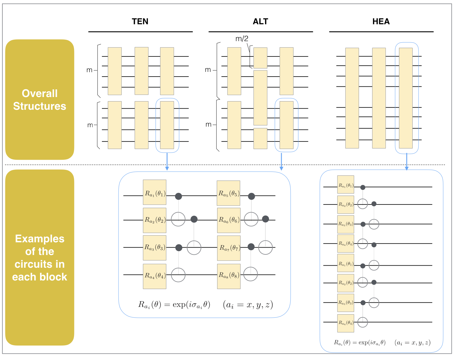
In Fig. 1, we show examples of the structures of these ansatzes.
Refer to caption
Figure 1: Examples of TEN, ALT, and HEA introduced in Section 2.2. The upper figures are the overall structures of the ansatzes in the case n=8n=8 and =3\ell=3 (and m=4m=4 for TEN and ALT). The circuits inside the blocks are exemplified in the lower figure, where σai\sigma_{a_{i}} (ai{x,y,z}a_{i}\in\{x,y,z\}) is the Pauli matrix operating on a qubit and θi[0,2π]\theta_{i}\in[0,2\pi] is the parameter.

3 Expressibility of the circuit ansatzes

In this section, we give some analytical expressions as well as upper bounds of the first and the second frame potentials of the three ansatzes introduced in Section 2.2, showing that the shallow ALT has almost the same expressibility as that of HEA. This result will be further confirmed by a numerical simulation in terms of the KL-divergence.

3.1 Analytical expression of the frame potential of the ansatzes

First of all, to compute the frame potentials of each ansatz, we assume that the ensemble of the unitary matrices corresponding to CHEA,nC_{\rm HEA}^{\ell,n} is 2-design. Similarly, the ensemble of the unitary matrices corresponding to each block of CALT,m,nC_{\rm ALT}^{\ell,m,n} and CTEN,m,nC_{\rm TEN}^{\ell,m,n} are assumed to be 2-design. These assumptions are also adopted in the discussion of [4] and [8]. Such ensemble of unitary matrices can be generated by randomly choosing the parameters of the circuit having a specific structure.

Before going into the detail, we show some integration formulae for random unitary matrices [15]. First, if the ensemble of n×nn\times n unitary matrices {U}\{U\} is 1-design, the following formula holds:

1designdUUijUmk=δimδjkn\displaystyle\int_{\rm 1design}dUU_{ij}U_{mk}^{*}=\frac{\delta_{im}\delta_{jk}}{n} , (4)

where 1design𝑑U\int_{\rm 1design}dU is the integral over the 1-design ensemble of the unitary matrices. Second, if the ensemble of n×nn\times n unitary matrices {U}\{U\} is 2-design, the following formula holds:

2designdUUi1j1Ui2j2Ui1j1Ui2j2=k=14λk(n)Δi1j1i2j2i1j1i2j2k,\displaystyle\int_{\rm 2design}dUU_{i_{1}j_{1}}U_{i_{2}j_{2}}U_{i_{1}^{\prime}j_{1}^{\prime}}^{\ast}U_{i_{2}^{\prime}j_{2}^{\prime}}^{\ast}=\sum_{k=1}^{4}\lambda_{k}^{(n)}\Delta^{k}_{i_{1}j_{1}i_{2}j_{2}i_{1}^{\prime}j_{1}^{\prime}i_{2}^{\prime}j_{2}^{\prime}}, (5)

where

λ1(n)=λ2(n)=122n1\displaystyle\lambda_{1}^{(n)}=\lambda_{2}^{(n)}=\frac{1}{2^{2n}-1} ,λ3(n)=λ4(n)=1(22n1)2n,\displaystyle,~~\lambda_{3}^{(n)}=\lambda_{4}^{(n)}=-\frac{1}{(2^{2n}-1)2^{n}},
Δi1j1i2j2i1j1i2j21\displaystyle\Delta^{1}_{i_{1}j_{1}i_{2}j_{2}i_{1}^{\prime}j_{1}^{\prime}i_{2}^{\prime}j_{2}^{\prime}} =δi1i1δj1j1δi2i2δj2j2,\displaystyle=\delta_{i_{1}i_{1}^{\prime}}\delta_{j_{1}j_{1}^{\prime}}\delta_{i_{2}i_{2}^{\prime}}\delta_{j_{2}j_{2}^{\prime}},
Δi1j1i2j2i1j1i2j22\displaystyle\Delta^{2}_{i_{1}j_{1}i_{2}j_{2}i_{1}^{\prime}j_{1}^{\prime}i_{2}^{\prime}j_{2}^{\prime}} =δi1i2δj1j2δi2i1δj2j1,\displaystyle=\delta_{i_{1}i_{2}^{\prime}}\delta_{j_{1}j_{2}^{\prime}}\delta_{i_{2}i_{1}^{\prime}}\delta_{j_{2}j_{1}^{\prime}},
Δi1j1i2j2i1j1i2j23\displaystyle\Delta^{3}_{i_{1}j_{1}i_{2}j_{2}i_{1}^{\prime}j_{1}^{\prime}i_{2}^{\prime}j_{2}^{\prime}} =δi1i1δj1j2δi2i2δj2j1,\displaystyle=\delta_{i_{1}i_{1}^{\prime}}\delta_{j_{1}j_{2}^{\prime}}\delta_{i_{2}i_{2}^{\prime}}\delta_{j_{2}j_{1}^{\prime}},
Δi1j1i2j2i1j1i2j24\displaystyle\Delta^{4}_{i_{1}j_{1}i_{2}j_{2}i_{1}^{\prime}j_{1}^{\prime}i_{2}^{\prime}j_{2}^{\prime}} =δi1i2δj1j1δi2i1δj2j2,\displaystyle=\delta_{i_{1}i_{2}^{\prime}}\delta_{j_{1}j_{1}^{\prime}}\delta_{i_{2}i_{1}^{\prime}}\delta_{j_{2}j_{2}^{\prime}}, (6)

and 2design𝑑U\int_{\rm 2design}dU is the integral over the 2-design ensemble of the unitary matrices. These formulae are effectively used to derive the theorems shown below.

The First Frame Potential

For the first frame potentials, the following theorem holds.

Theorem 1.

If the ensemble of the unitary matrices corresponding to CHEA,nC_{\rm HEA}^{\ell,n} and the ensemble of the unitary matrices corresponding to each block of CALT,m,nC_{\rm ALT}^{\ell,m,n} and CTEN,m,nC_{\rm TEN}^{\ell,m,n} are 2-design, then the following equalities hold:

(1)(CHEA,n)=(1)(CALT,m,n)=(1)(CTEN,m,n)=Haar(1)(2n).\displaystyle\mathcal{F}^{(1)}(C_{\rm HEA}^{\ell,n})=\mathcal{F}^{(1)}(C_{\rm ALT}^{\ell,m,n})=\mathcal{F}^{(1)}(C_{\rm TEN}^{\ell,m,n})=\mathcal{F}^{(1)}_{\rm Haar}(2^{n}). (7)

The equality, (1)(CHEA,n)=Haar(1)(2n)\mathcal{F}^{(1)}(C_{\rm HEA}^{\ell,n})=\mathcal{F}^{(1)}_{\rm Haar}(2^{n}), can be readily proved from the assumption of the theorem, because, if the ensemble of the unitary matrices corresponding to the circuit is 2-design, the ensemble of the states generated by the circuit is a state 2-design (and therefore a state 1-design). For the other equalities, the proof is given in Appendix. Note that, accordingly, the ensembles of the states generated by CHEA,nC_{\rm HEA}^{\ell,n}, CALT,m,nC_{\rm ALT}^{\ell,m,n}, and CTEN,m,nC_{\rm TEN}^{\ell,m,n} are all 1-design.

The Second Frame Potential

The second frame potential of the Haar random circuits, Haar(2)(2n)\mathcal{F}^{(2)}_{\rm Haar}(2^{n}), can be computed as

Haar(2)(2n)=01dFF2(2n1)(1F)2n2\displaystyle\qquad\mathcal{F}^{(2)}_{\rm Haar}(2^{n})=\int_{0}^{1}dFF^{2}(2^{n}-1)(1-F)^{2^{n}-2} =1(2n+1)2n1.\displaystyle=\frac{1}{(2^{n}+1)2^{n-1}}. (8)

Then, for CHEA,nC_{\rm HEA}^{\ell,n} and CTEN,m,nC_{\rm TEN}^{\ell,m,n}, the following theorem holds.

Theorem 2.

If the ensemble of the unitary matrices corresponding to CHEA,nC_{\rm HEA}^{\ell,n} and the ensemble of the unitary matrices corresponding to each block of CTEN,m,nC_{\rm TEN}^{\ell,m,n} are 2-design, then the following equalities hold:

(2)(CHEA,n)\displaystyle\mathcal{F}^{(2)}(C_{\rm HEA}^{\ell,n}) =Haar(2)(2n),\displaystyle=\mathcal{F}^{(2)}_{\rm Haar}(2^{n}), (9)
(2)(CTEN,m,n)\displaystyle\mathcal{F}^{(2)}(C_{\rm TEN}^{\ell,m,n}) =2nm12n+1(2m+1)nmHaar(2)(2n).\displaystyle=2^{\frac{n}{m}-1}\cdot\frac{2^{n}+1}{(2^{m}+1)^{\frac{n}{m}}}\mathcal{F}^{(2)}_{\rm Haar}(2^{n}). (10)

The equality (9) is readily proved from the assumption of the theorem, because, as we mentioned above, if the ensemble of the unitary matrices corresponding to the circuit is 2-design, the ensemble of the states generated by the circuit is a state 2-design. For Eq.(10), we give the proof in Appendix. From this theorem we find that (2)(CTEN,m,n)\mathcal{F}^{(2)}(C_{\rm TEN}^{\ell,m,n}) is always larger than Haar(2)(2n)\mathcal{F}^{(2)}_{\rm Haar}(2^{n}); in particular, (2)(CTEN,m,n)2n/m1Haar(2)(2n)\mathcal{F}^{(2)}(C_{\rm TEN}^{\ell,m,n})\simeq 2^{n/m-1}\mathcal{F}^{(2)}_{\rm Haar}(2^{n}) for large nn, meaning that the expressibility of TEN is much smaller than that of HEA in the sense of the frame potential.

As for ALT, it is difficult to obtain an explicit formula like the case of HEA and TEN. Hence in Theorem 3 below, we provide a formula for computing the values of (2)(CALT2,m,n)\mathcal{F}^{(2)}(C_{\rm ALT}^{2,m,n}) and (2)(CALT3,m,n)\mathcal{F}^{(2)}(C_{\rm ALT}^{3,m,n}); the computation methods for the other \ells are left for future work. Before stating the theorem, below we define a 16-dimensional vector 𝐚(2,m){\bf a}(2,m), a 16×1616\times 16 matrix B(2,m)B(2,m), a 64-dimensional vector 𝐚(3,m){\bf a}(3,m), and a 64×6464\times 64 matrix B(3,m)B(3,m). Given integers ka,kb{1,2,3,4}k_{a},k_{b}\in\{1,2,3,4\}, the (4(ka1)+kb)(4(k_{a}-1)+k_{b})-th component of the vector 𝐚(2,m){\bf a}(2,m) is defined as

𝐚(2,m)4(ka1)+kb\displaystyle{\bf a}(2,m)_{4(k_{a}-1)+k_{b}} =2designdP𝑑Qλka(m)λkb(m)Δ(ka,kb)(P,Q),\displaystyle=\int_{\rm 2design}dPdQ\sqrt{\lambda_{k_{a}}^{(m)}\lambda_{k_{b}}^{(m)}}\Delta^{(k_{a},k_{b})}(P,Q), (11)

where Δ(ka,kb)(P,Q)\Delta^{(k_{a},k_{b})}(P,Q) is the function of m/2×m/2m/2\times m/2 unitary matrices PP and QQ:

Δ(ka,kb)(P,Q)\displaystyle\Delta^{(k_{a},k_{b})}(P,Q) =uuiijjllppqqΔu0u0i0i0kaΔp0p0q0q0kbPjuPjuPliPliQlpQlpQjqQjq.\displaystyle=\sum_{\begin{subarray}{c}uu^{\prime}ii^{\prime}\\ jj^{\prime}ll^{\prime}\end{subarray}}\sum_{\begin{subarray}{c}pp^{\prime}qq^{\prime}\end{subarray}}\Delta^{k_{a}}_{u0u^{\prime}0i0i^{\prime}0}\Delta^{k_{b}}_{p0p^{\prime}0q0q^{\prime}0}P_{ju}P_{j^{\prime}u^{\prime}}P_{li}^{\ast}P_{l^{\prime}i^{\prime}}^{\ast}Q_{lp}Q_{l^{\prime}p^{\prime}}Q_{jq}^{\ast}Q_{j^{\prime}q^{\prime}}^{\ast}. (12)

Next, given integers ka,kb,kc{1,2,3,4}k_{a},k_{b},k_{c}\in\{1,2,3,4\}, the (16(ka1)+4(kb1)+kc)(16(k_{a}-1)+4(k_{b}-1)+k_{c})-th component of the vector 𝐚(3,m){\bf a}(3,m) is defined as

𝐚(3,m)16(ka1)+4(kb1)+kc\displaystyle{\bf a}(3,m)_{16(k_{a}-1)+4(k_{b}-1)+k_{c}} =2designdP𝑑Qλka(m)λkb(m)λkc(m)Δ(ka,kb,kc)(P,Q),\displaystyle=\int_{\rm 2design}dPdQ\sqrt{\lambda_{k_{a}}^{(m)}\lambda_{k_{b}}^{(m)}\lambda_{k_{c}}^{(m)}}\Delta^{(k_{a},k_{b},k_{c})}(P,Q), (13)

where Δ(ka,kb,kc)(P,Q)\Delta^{(k_{a},k_{b},k_{c})}(P,Q) is a function of m/2×m/2m/2\times m/2 unitary matrices PP and QQ:

Δ(ka,kb,kc)(P,Q)\displaystyle\Delta^{(k_{a},k_{b},k_{c})}(P,Q) =uuiijjllrrttppqqΔu0u0i0i0kaΔjljltrtrkbΔp0p0q0q0kcPtuPtuPjiPjiQlpQlpQrqQrq.\displaystyle=\sum_{\begin{subarray}{c}uu^{\prime}ii^{\prime}\\ jj^{\prime}ll^{\prime}\end{subarray}}\sum_{\begin{subarray}{c}rr^{\prime}tt^{\prime}\\ pp^{\prime}qq^{\prime}\end{subarray}}\Delta^{k_{a}}_{u0u^{\prime}0i0i^{\prime}0}\Delta^{k_{b}}_{jlj^{\prime}l^{\prime}trt^{\prime}r^{\prime}}\Delta^{k_{c}}_{p0p^{\prime}0q0q^{\prime}0}P_{tu}P_{t^{\prime}u^{\prime}}P_{ji}^{\ast}P_{j^{\prime}i^{\prime}}^{\ast}Q_{lp}Q_{l^{\prime}p^{\prime}}Q_{rq}^{\ast}Q_{r^{\prime}q^{\prime}}^{\ast}. (14)

Also, given integers ka,kb,kc,kd{1,2,3,4}k_{a},k_{b},k_{c},k_{d}\in\{1,2,3,4\}, the (4(ka1)+4kb,4(kc1)+kd)(4(k_{a}-1)+4k_{b},4(k_{c}-1)+k_{d})-th component of the matrix B(m,2)B(m,2) is defined as

B(2,m)4(ka1)+kb,4(kc1)+kd\displaystyle B(2,m)_{4(k_{a}-1)+k_{b},4(k_{c}-1)+k_{d}} =2designdP𝑑Qλka(m)λkb(m)λkc(m)λkd(m)Δ(ka,kb,kc,kd)(P,Q),\displaystyle=\int_{\rm 2design}dPdQ\sqrt{\lambda_{k_{a}}^{(m)}\lambda_{k_{b}}^{(m)}}\sqrt{\lambda_{k_{c}}^{(m)}\lambda_{k_{d}}^{(m)}}\Delta^{(k_{a},k_{b},k_{c},k_{d})}(P,Q), (15)

where Δ(ka,kb,kc,kd)(P,Q)\Delta^{(k_{a},k_{b},k_{c},k_{d})}(P,Q) is a function of m×mm\times m matrices PP and QQ:

Δ(ka,kb,kc,kd)(P,Q)\displaystyle\Delta^{(k_{a},k_{b},k_{c},k_{d})}(P,Q) =u2u2i2i2j2j2l2l2p2p2q2q2u3u3i3i3j3j3l3l3p3p3q3q3Δu20u20i20i20kaΔp20p20q20q20kbΔu30u30i30i30kcΔp30p30q30q30kd\displaystyle=\sum_{\begin{subarray}{c}u_{2}u^{\prime}_{2}i_{2}i^{\prime}_{2}\\ j_{2}j^{\prime}_{2}l_{2}l^{\prime}_{2}\end{subarray}}\sum_{\begin{subarray}{c}p_{2}p^{\prime}_{2}q_{2}q^{\prime}_{2}\end{subarray}}\sum_{\begin{subarray}{c}u_{3}u^{\prime}_{3}i_{3}i^{\prime}_{3}\\ j_{3}j^{\prime}_{3}l_{3}l^{\prime}_{3}\end{subarray}}\sum_{\begin{subarray}{c}p_{3}p^{\prime}_{3}q_{3}q^{\prime}_{3}\end{subarray}}\Delta^{k_{a}}_{u_{2}0u^{\prime}_{2}0i_{2}0i^{\prime}_{2}0}\Delta^{k_{b}}_{p_{2}0p^{\prime}_{2}0q_{2}0q^{\prime}_{2}0}\Delta^{k_{c}}_{u_{3}0u^{\prime}_{3}0i_{3}0i^{\prime}_{3}0}\Delta^{k_{d}}_{p_{3}0p^{\prime}_{3}0q_{3}0q^{\prime}_{3}0}
×Pj2u2j3u3Pj2u2j3u3Pl2i2l3i3Pl2i2l3i3Ql2p2l3p3Ql2p2l3p3Qj2q2j3q3Qj2q2j3q3\displaystyle\qquad\times P_{j_{2}u_{2}}^{j_{3}u_{3}}P_{j^{\prime}_{2}u^{\prime}_{2}}^{j^{\prime}_{3}u^{\prime}_{3}}P_{l_{2}i_{2}}^{\ast l_{3}i_{3}}P_{l^{\prime}_{2}i^{\prime}_{2}}^{\ast l^{\prime}_{3}i^{\prime}_{3}}Q_{l_{2}p_{2}}^{l_{3}p_{3}}Q_{l^{\prime}_{2}p^{\prime}_{2}}^{l^{\prime}_{3}p^{\prime}_{3}}Q_{j_{2}q_{2}}^{\ast j_{3}q_{3}}Q_{j_{2}^{\prime}q^{\prime}_{2}}^{\ast j_{3}^{\prime}q^{\prime}_{3}} (16)

For the matrix component Mi,js,tM^{s,t}_{i,j}, the upper indices correspond to the first m/2m/2 qubits and the lower indices correspond to the last m/2m/2. Given integers ka,kb,kc,kd,ke,kf{1,2,3,4}k_{a},k_{b},k_{c},k_{d},k_{e},k_{f}\in\{1,2,3,4\}, the (16(ka1)+4(kb1)+kc,16(kd1)+4(ke1)+kf)(16(k_{a}-1)+4(k_{b}-1)+k_{c},16(k_{d}-1)+4(k_{e}-1)+k_{f})-th component of the matrix B(m,3)B(m,3) is defined as

B(3,m)\displaystyle B(3,m) 16(ka1)+4(kb1)+kc,16(kd1)+4(ke1)+kf{}_{16(k_{a}-1)+4(k_{b}-1)+k_{c},16(k_{d}-1)+4(k_{e}-1)+k_{f}}
=2designdP𝑑Qλka(m)λkb(m)λkc(m)λkd(m)λke(m)λkf(m)Δ(ka,kb,kc,kd,ke,kf)(P,Q),\displaystyle=\int_{\rm 2design}dPdQ\sqrt{\lambda_{k_{a}}^{(m)}\lambda_{k_{b}}^{(m)}\lambda_{k_{c}}^{(m)}}\sqrt{\lambda_{k_{d}}^{(m)}\lambda_{k_{e}}^{(m)}\lambda_{k_{f}}^{(m)}}\Delta^{(k_{a},k_{b},k_{c},k_{d},k_{e},k_{f})}(P,Q), (17)

where Δ(ka,kb,kc,kd,ke,kf)(P,Q)\Delta^{(k_{a},k_{b},k_{c},k_{d},k_{e},k_{f})}(P,Q) is a function of m×mm\times m matrices PP and QQ:

Δ(ka,kb,kc,kd,ke,kf)(P,Q)\displaystyle\Delta^{(k_{a},k_{b},k_{c},k_{d},k_{e},k_{f})}(P,Q) =u2u2i2i2j2j2l2l2r2r2t2t2p2p2q2q2u3u3i3i3j3j3l3l3r3r3t3t3p3p3q3q3Δu20u20i20i20k11aΔj2l2j2l2t2r2t2r2k31aΔp20p2q20q20k11b\displaystyle=\sum_{\begin{subarray}{c}u_{2}u^{\prime}_{2}i_{2}i^{\prime}_{2}\\ j_{2}j^{\prime}_{2}l_{2}l^{\prime}_{2}\end{subarray}}\sum_{\begin{subarray}{c}r_{2}r^{\prime}_{2}t_{2}t^{\prime}_{2}\\ p_{2}p^{\prime}_{2}q_{2}q^{\prime}_{2}\end{subarray}}\sum_{\begin{subarray}{c}u_{3}u^{\prime}_{3}i_{3}i^{\prime}_{3}\\ j_{3}j^{\prime}_{3}l_{3}l^{\prime}_{3}\end{subarray}}\sum_{\begin{subarray}{c}r_{3}r^{\prime}_{3}t_{3}t^{\prime}_{3}\\ p_{3}p^{\prime}_{3}q_{3}q^{\prime}_{3}\end{subarray}}\Delta^{k_{11}^{a}}_{u_{2}0u^{\prime}_{2}0i_{2}0i^{\prime}_{2}0}\Delta^{k_{31}^{a}}_{j_{2}l_{2}j^{\prime}_{2}l^{\prime}_{2}t_{2}r_{2}t^{\prime}_{2}r^{\prime}_{2}}\Delta^{k_{11}^{b}}_{p_{2}0p^{\prime}_{2}q_{2}0q^{\prime}_{2}0}
×Δu30u30i30i30k12aΔj3l3j3l3t3r3t3r3k32aΔp30p3q30q30k12bPt2u2t3u3Pt2u2t3u3Pj2i2j3i3Pj2i2j3i3\displaystyle\qquad\times\Delta^{k_{12}^{a}}_{u_{3}0u^{\prime}_{3}0i_{3}0i^{\prime}_{3}0}\Delta^{k_{32}^{a}}_{j_{3}l_{3}j^{\prime}_{3}l^{\prime}_{3}t_{3}r_{3}t^{\prime}_{3}r^{\prime}_{3}}\Delta^{k_{12}^{b}}_{p_{3}0p^{\prime}_{3}q_{3}0q^{\prime}_{3}0}P_{t_{2}u_{2}}^{t_{3}u_{3}}P_{t^{\prime}_{2}u^{\prime}_{2}}^{t^{\prime}_{3}u^{\prime}_{3}}P^{\ast j_{3}i_{3}}_{j_{2}i_{2}}P^{\ast j^{\prime}_{3}i^{\prime}_{3}}_{j^{\prime}_{2}i^{\prime}_{2}}
×Ql2p2l3p3Ql2p2l3p3Qr2q2r3q3Qr2q2r3q3.\displaystyle\qquad\times Q_{l_{2}p_{2}}^{l_{3}p_{3}}Q_{l^{\prime}_{2}p^{\prime}_{2}}^{l^{\prime}_{3}p^{\prime}_{3}}Q^{\ast r_{3}q_{3}}_{r_{2}q_{2}}Q^{\ast r^{\prime}_{3}q^{\prime}_{3}}_{r^{\prime}_{2}q^{\prime}_{2}}. (18)

Now we can give the theorem as follows (the proof is given in Appendix).

Theorem 3.

If the ensemble of the unitary matrices corresponding to each block of CALT2,m,nC_{\rm ALT}^{2,m,n} and CALT3,m,nC_{\rm ALT}^{3,m,n} are 2-design, then we have

(2)(CALT2,m,n)=𝐚(2,m)TB(2,m)nm1𝐚(2,m),\displaystyle\mathcal{F}^{(2)}(C_{\rm ALT}^{2,m,n})={\bf a}(2,m)^{\rm T}B(2,m)^{\frac{n}{m}-1}{\bf a}(2,m), (19)
(2)(CALT3,m,n)=𝐚(3,m)TB(3,m)nm1𝐚(3,m).\displaystyle\mathcal{F}^{(2)}(C_{\rm ALT}^{3,m,n})={\bf a}(3,m)^{\rm T}B(3,m)^{\frac{n}{m}-1}{\bf a}(3,m). (20)
Refer to caption
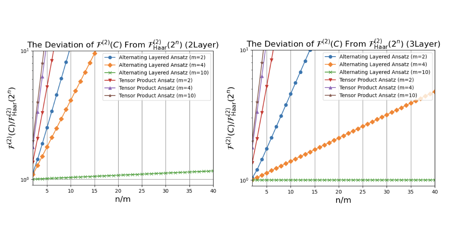
Figure 2: The values of (2)(C)/Haar(2)(2n)\mathcal{F}^{(2)}(C)/\mathcal{F}^{(2)}_{\rm Haar}(2^{n}) for ALT and TEN. The left and right figures show the case =2\ell=2 and =3\ell=3, respectively. The vertical axes are in the logarithmic scale. If (2)(C)/Haar(2)(2n)\mathcal{F}^{(2)}(C)/\mathcal{F}^{(2)}_{\rm Haar}(2^{n}) is close to 1, this means that the expressibility of the ansatz CC is relatively high.

The vectors 𝐚(,m){\bf a}(\ell,m) and the matrices B(,m)B(\ell,m) for =2,3\ell=2,3 are obtained by directly computing Eqs. (11), (13), (15), and (3.1), which then lead to (2)(CALT2,m,n)\mathcal{F}^{(2)}(C_{\rm ALT}^{2,m,n}) and (2)(CALT3,m,n)\mathcal{F}^{(2)}(C_{\rm ALT}^{3,m,n}). Now our interest is in the gap of these quantities from Haar(t)(2n)\mathcal{F}^{(t)}_{\rm Haar}(2^{n}), to see the expressibility of ALT. For this purpose, in Fig. 2 we show (2)(CALT2,m,n)/Haar(2)(2n)\mathcal{F}^{(2)}(C_{\rm ALT}^{2,m,n})/\mathcal{F}^{(2)}_{\rm Haar}(2^{n}) and (2)(CALT3,m,n)/Haar(2)(2n)\mathcal{F}^{(2)}(C_{\rm ALT}^{3,m,n})/\mathcal{F}^{(2)}_{\rm Haar}(2^{n}) as a function of n/mn/m, for several values of (m,n)(m,n). For comparison, (2)(CTEN2,m,n)/Haar(2)(2n)\mathcal{F}^{(2)}(C_{\rm TEN}^{2,m,n})/\mathcal{F}^{(2)}_{\rm Haar}(2^{n}) and (2)(CTEN3,m,n)/Haar(2)(2n)\mathcal{F}^{(2)}(C_{\rm TEN}^{3,m,n})/\mathcal{F}^{(2)}_{\rm Haar}(2^{n}) are shown in the figure. Recall that, if this measure takes a smaller value, this means that the corresponding ansatz has a higher expressibility. Here is the list of notable points:

  • For any pair of (n,m)(n,m), it is clear that (2)(CALT,m,n)\mathcal{F}^{(2)}(C_{\rm ALT}^{\ell,m,n}) is much smaller than (2)(CTEN,m,n)\mathcal{F}^{(2)}(C_{\rm TEN}^{\ell,m,n}) for both =2,3\ell=2,3. This means that, as expected, ALT has a much higher expressibility than TEN.

  • For any pair of (n,m)(n,m), (2)(CALT2,m,n)>(2)(CALT3,m,n)\mathcal{F}^{(2)}(C_{\rm ALT}^{2,m,n})>\mathcal{F}^{(2)}(C_{\rm ALT}^{3,m,n}) hold, i.e., as \ell increases, the expressibility increases.

  • For any fixed n/mn/m, the ALT with bigger mm always has a higher expressibility. For instance, the ALT with (n,m)=(50,10)(n,m)=(50,10) has a higher expressibility than the ALT with (n,m)=(20,4)(n,m)=(20,4). This is simply because, if the structure of the circuit (the number of division in each layer for making the block) is the same, then an ALT with bigger block components has a higher expressibility.

  • For a fixed nn, we have ALT with the smaller second order frame potential by taking mm bigger. For instance n=100n=100, we have (2)(CALT2,2,100)>(2)(CALT2,4,100)>(2)(CALT2,10,100){\mathcal{F}}^{(2)}(C_{\rm ALT}^{2,2,100})>{\mathcal{F}}^{(2)}(C_{\rm ALT}^{2,4,100})>{\mathcal{F}}^{(2)}(C_{\rm ALT}^{2,10,100}). That is, for a limited number of available qubits, the ALT with less blocks has a higher expressibility.

  • (2)(CALT,m,n)Haar(2)(2n)\mathcal{F}^{(2)}(C_{\rm ALT}^{\ell,m,n})\simeq\mathcal{F}^{(2)}_{\rm Haar}(2^{n}) when m=10m=10 for all n/mn/m within the figure and for both =2,3\ell=2,3. Hence the ALT composed from the blocks with m=10m=10 qubits in each layer has almost the same expressibility as the HEA without respect to the total qubits number, nn. In other words, for a given HEA with fixed nn, we can divide each layer into separated 10-qubits blocks to make an ALT, without decreasing the expressibility.

The last point is of particular important in our scenario. That is, we are concerned with the condition on the number mm such that (2)(CALT,m,n)Haar(2)(2n)\mathcal{F}^{(2)}(C_{\rm ALT}^{\ell,m,n})\simeq\mathcal{F}^{(2)}_{\rm Haar}(2^{n}) holds. The following Theorem 4 and the subsequent Corollary 1, which can be readily derived from the theorem, provide a means for evaluating such mm.

Theorem 4.

If the ensemble of the unitary matrices corresponding to each block of CALT2,m,nC_{\rm ALT}^{2,m,n} and CALT3,m,nC_{\rm ALT}^{3,m,n} are 2-design, then the following inequalities hold:

(2)(CALT2,m,n)\displaystyle\mathcal{F}^{(2)}(C_{\rm ALT}^{2,m,n}) <(1+12n)(1+1.22m)2(1+8((1+20.82m/2)nm11))Haar(2)(2n),\displaystyle<\left(1+\frac{1}{2^{n}}\right)\left(1+\frac{1.2}{2^{m}}\right)^{2}\left(1+8\left(\left(1+\frac{20.8}{2^{m/2}}\right)^{\frac{n}{m}-1}-1\right)\right)\mathcal{F}^{(2)}_{\rm Haar}(2^{n}), (21)
(2)(CALT3,m,n)\displaystyle\mathcal{F}^{(2)}(C_{\rm ALT}^{3,m,n}) <(1+12n)(1+1.22m)2(1+32((1+83.22m/2)nm11))Haar(2)(2n).\displaystyle<\left(1+\frac{1}{2^{n}}\right)\left(1+\frac{1.2}{2^{m}}\right)^{2}\left(1+32\left(\left(1+\frac{83.2}{2^{m/2}}\right)^{\frac{n}{m}-1}-1\right)\right)\mathcal{F}^{(2)}_{\rm Haar}(2^{n}). (22)
Corollary 1.

If m=2alog2nm=2a\log_{2}n and 143/(ana1log2n)<1143/(an^{a-1}\log_{2}n)<1,

(2)(CALT2,m,n)\displaystyle\mathcal{F}^{(2)}(C_{\rm ALT}^{2,m,n}) <(1+12n)(1+1.2n2a)2(1+143ana1log2n)Haar(2)(2n).\displaystyle<\left(1+\frac{1}{2^{n}}\right)\left(1+\frac{1.2}{n^{2a}}\right)^{2}\left(1+\frac{143}{an^{a-1}\log_{2}n}\right)\mathcal{F}^{(2)}_{\rm Haar}(2^{n}). (23)

If m=2alog2nm=2a\log_{2}n and 2288/(ana1log2n)<12288/(an^{a-1}\log_{2}n)<1,

(2)(CALT3,m,n)\displaystyle\mathcal{F}^{(2)}(C_{\rm ALT}^{3,m,n}) <(1+12n)(1+1.2n2a)2(1+2288ana1log2n)Haar(2)(2n).\displaystyle<\left(1+\frac{1}{2^{n}}\right)\left(1+\frac{1.2}{n^{2a}}\right)^{2}\left(1+\frac{2288}{an^{a-1}\log_{2}n}\right)\mathcal{F}^{(2)}_{\rm Haar}(2^{n}). (24)

Recall from Eq. (2) that (t)(C)Haar(t)(N)\mathcal{F}^{(t)}(C)\geq\mathcal{F}^{(t)}_{\rm Haar}(N) holds for any ansatz CC. Therefore, if m4lognm\geq 4\log n and nn is enough large, Corollary 1 implies that (2)(CALT2,m,n)Haar(2)(2n)\mathcal{F}^{(2)}(C_{\rm ALT}^{2,m,n})\sim\mathcal{F}^{(2)}_{\rm Haar}(2^{n}) and (2)(CALT3,m,n)Haar(2)(2n)\mathcal{F}^{(2)}(C_{\rm ALT}^{3,m,n})\sim\mathcal{F}^{(2)}_{\rm Haar}(2^{n}). This means that the ensembles of the states generated by CALT2,m,nC_{\rm ALT}^{2,m,n} and CALT3,m,nC_{\rm ALT}^{3,m,n} are almost 2-design. Hence in this case, from Theorem 2, the expressibility of ALT is as high as that of HAE. It is worth mentioning that, when m=O(log2n)m=O(\log_{2}n), the vanishing gradient problem does not happen in ALT as long as the cost function is local and \ell is small [8]. More precisely, it was shown there that the variance of the gradient of such a cost function is larger than the value proportional to O(1/2m)O(1/2^{m\ell}); thus, by taking m=O(log2n)m=O(\log_{2}n), the variance decreases with only O(1/poly(n))O(1/{\rm poly}(n)) as a function of nn, whereas in the HEA case the same variance decreases exponentially fast as nn becomes large. Therefore, the expressibility and the trainability coexists in the shallow ALT with m=O(log2n)m=O(\log_{2}n).

3.2 Expressibility measured by KL divergence

nn Ansatz \ell mm
Depth of
each block
# of gate
parameters
Example of
the circuit
4 TEN 2 2 2 16 -
3 2 2 24 Fig. 3
ALT 2 2 2 16 -
3 2 2 24 Fig. 3
HEA 4 - - 16 Fig. 3
6 TEN 2 2 2 24 -
3 2 2 36 -
ALT 2 2 2 24 -
3 2 2 36 -
HEA 6 - - 36 -
8 TEN 2 2 2 32 -
4 4 64 -
3 2 2 48 -
4 4 96 -
ALT 2 2 2 32 -
4 4 64 -
3 2 2 48 -
4 4 96 -
HEA 8 - - 64 -
Table 1: Parameters chosen for computing the KL-divergence. The number of gate parameters are computed by n××(Depthofeachblock)n\times\ell\times{\rm(Depth\ of\ each\ block)} for TEN and ALT, and n×n\times\ell for HEA.

In Subsection 3.1, we have shown that the first two moments of P(CALT,m,n,F)P(C_{\rm ALT}^{\ell,m,n},F) and P(CHEA,n,F)P(C_{\rm HEA}^{\ell,n},F) are close to those of PHaar(F)P_{\rm Haar}(F), as long as m=O(log2n)m=O(\log_{2}n) and the block components of the ansatzes are sufficiently random. (Recall that, if every block is completely random, then the set of HEA constitutes the Haar ensemble.) The result implies that both P(CALT,m,n,F)P(C_{\rm ALT}^{\ell,m,n},F) and P(CHEA,n,F)P(C_{\rm HEA}^{\ell,n},F) are close to PHaar(F)P_{\rm Haar}(F) itself, meaning that P(CALT,m,n,F)P(CHEA,n,F)PHaar(F)P(C_{\rm ALT}^{\ell,m,n},F)\simeq P(C_{\rm HEA}^{\ell,n},F)\simeq P_{\rm Haar}(F). In this subsection, to support this conjecture, we evaluate the values of KL-divergence (C)=DKL(P(C,F)PHaar(F))\mathcal{E}(C)=D_{\mathrm{KL}}\left(P(C,F)\|P_{\mathrm{Haar}}(F)\right) for the case C=CALT,m,nC=C_{\rm ALT}^{\ell,m,n} and C=CHEA,nC=C_{\rm HEA}^{\ell,n}, in addition to C=CTEN,m,nC=C_{\rm TEN}^{\ell,m,n} for comparison with various sets of (,m,n)(\ell,m,n). Especially, we focus on the relationship between the values of (2)(C)\mathcal{F}^{(2)}(C) and (C)\mathcal{E}(C), and check if (2)(C)(2)(C)\mathcal{F}^{(2)}(C)\simeq\mathcal{F}^{(2)}(C^{\prime}) would lead to (C)(C)\mathcal{E}(C)\simeq\mathcal{E}(C^{\prime}) for a fixed nn.

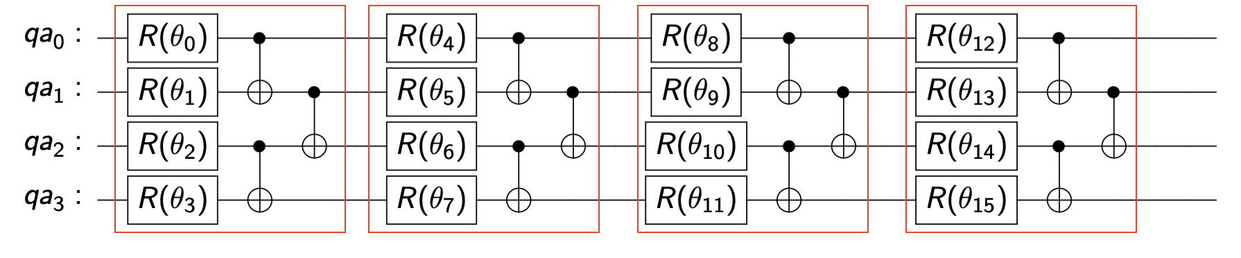
The parameters taken for calculating the KL-divergence are summarized in Table 1. Note that the circuits are chosen to be similar to those used in Section 3.1; for TEN and ALT, the depth of the circuits inside the blocks are all set to mm so that the ensemble of the unitary matrices corresponding to those circuits become close to 2-design [16, 17]; for HEA, \ell is set to nn so that the ensemble of the unitary matrices corresponding to the whole circuits becomes close to 2-design. It is expected that (2)(CALT3,2,4)(2)(CHEA4,4)\mathcal{F}^{(2)}(C_{\rm ALT}^{3,2,4})\approx\mathcal{F}^{(2)}(C_{\rm HEA}^{4,4}) and (2)(CALT3,4,8)(2)(CHEA8,8)\mathcal{F}^{(2)}(C_{\rm ALT}^{3,4,8})\approx\mathcal{F}^{(2)}(C_{\rm HEA}^{8,8}) are realized, because, in Fig 2, we see that (2)(CALT3,2,4)\mathcal{F}^{(2)}(C_{\rm ALT}^{3,2,4}) and (2)(CALT3,4,8)\mathcal{F}^{(2)}(C_{\rm ALT}^{3,4,8}) are almost equals to the Haar values when the ensembles of unitary matrices corresponding to each block are 2-design. Thus, we here check if (2)(C)(2)(C)\mathcal{F}^{(2)}(C)\simeq\mathcal{F}^{(2)}(C^{\prime}) would mean (C)(C)\mathcal{E}(C)\simeq\mathcal{E}(C^{\prime}) in these parameter sets. As an example of the circuit, the whole structure of CTEN3,2,4C_{\rm TEN}^{3,2,4}, CALT3,2,4C_{\rm ALT}^{3,2,4}, and CHEA4,4C_{\rm HEA}^{4,4} in our settings are shown in Figs. 3, 3, and 3, respectively. As illustrated in the figures, each layer is composed of parametrized single qubit gates and fixed 2-qubit CNOT gates.

In each trial of computing KL-divergence, we generate 200 states. When generating a state in each trial, we randomly choose the parameters and the type fo single-qubit gate of the circuit. That is, for the ii-th single qubit gate Ri(θi)=exp(σaiθi)R_{i}(\theta_{i})=\exp(\sigma_{a_{i}}\theta_{i}) with ai={x,y,z}a_{i}=\{x,y,z\} and θi[0,2π]\theta_{i}\in[0,2\pi], in each trial all aia_{i} and θi\theta_{i} are randomly chosen. Then 200 fidelity values are computed, which are then used to construct the histogram with 1000 bins to approximate the probability distribution P(C,F)P(C,F). Note that increasing the number of generated states and the number of bins do not affect the following conclusions.

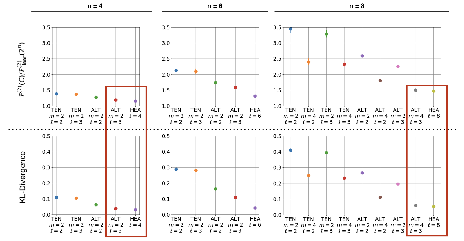
In this setting, Fig. 4 shows the KL divergences (CALT,m,n)\mathcal{E}(C_{\rm ALT}^{\ell,m,n}), (CHEA,n)\mathcal{E}(C_{\rm HEA}^{\ell,n}), and (CTEN,m,n)\mathcal{E}(C_{\rm TEN}^{\ell,m,n}). As a reference, we also show the values of (2)(C)/Haar(2)(2n)\mathcal{F}^{(2)}(C)/\mathcal{F}^{(2)}_{\rm Haar}(2^{n}) computed from the second moment of the fidelity distributions. Each data point and associated error bar is the average and the standard deviation of 10 trials of computation, respectively. Here is the list of points:

  • For a fixed nn, (CTEN,m,n)\mathcal{E}(C_{\rm TEN}^{\ell,m,n}) is always bigger than (CALT,m,n)\mathcal{E}(C_{\rm ALT}^{\ell,m,n}) and (CHEA,n)\mathcal{E}(C_{\rm HEA}^{\ell,n}).

  • As the number of layers increases, the KL-divergence decreases for fixed (m,n)(m,n).

  • For a fixed nn, the tendency of the values of (2)(C)/Haar(2)(2n)\mathcal{F}^{(2)}(C)/\mathcal{F}^{(2)}_{\rm Haar}(2^{n}) is strongly correlated with that of KL-divergence.

  • As expected, (2)(CALT3,m,n)(2)(CHEAn,n)\mathcal{F}^{(2)}(C_{\rm ALT}^{3,m,n})\approx\mathcal{F}^{(2)}(C_{\rm HEA}^{n,n}) is realized when (m,n)=(2,4)(m,n)=(2,4) and (4,8)(4,8).

  • (CALT3,m,n)\mathcal{E}(C_{\rm ALT}^{3,m,n}) is as small as (CHEAn,n)\mathcal{E}(C_{\rm HEA}^{n,n}) in the parameter sets where (2)(CALT3,m,n)(2)(CHEAn,n)\mathcal{F}^{(2)}(C_{\rm ALT}^{3,m,n})\approx\mathcal{F}^{(2)}(C_{\rm HEA}^{n,n}) is realized, i.e., (m,n)=(2,4)(m,n)=(2,4) and (4,8)(4,8). This result implies that the state distribution in ALT is also close to that in HEA, in the setting where the second frame potential is close to Haar(2)(2n)\mathcal{F}^{(2)}_{\rm Haar}(2^{n}).

From some of the above observations, we find the strong correlation between (2)(C)/Haar(2)(2n)\mathcal{F}^{(2)}(C)/\mathcal{F}^{(2)}_{\rm Haar}(2^{n}) and (C)\mathcal{E}(C); that is, as (2)(C)\mathcal{F}^{(2)}(C) becomes close to 11, then (C)\mathcal{E}(C) becomes close to 00. Therefore, combining the result obtained in Section 3.1, we get a clear evidence that, as far as m=O(log2n)m=O(\log_{2}n), (CALT2,m,n)0\mathcal{E}(C_{\rm ALT}^{2,m,n})\approx 0 and (CALT3,m,n)0\mathcal{E}(C_{\rm ALT}^{3,m,n})\approx 0 hold. That is, the high expressibility and trainability in ALT proven in Section 3.1 are assured also in terms of KL-divergence.

Refer to caption
(a) The structure of CTEN3,2,4C_{\rm TEN}^{3,2,4}. The red boxes correspond to blocks.
Refer to caption
(b) The structure of CALT3,2,4C_{\rm ALT}^{3,2,4}. The red boxes correspond to blocks.
Refer to caption
(c) The structure of CHEA4,4C_{\rm HEA}^{4,4}.
Figure 3: The structures of ansatzes in our setting.
Refer to caption
Figure 4: (2)(C)/Haar(2)(2n)\mathcal{F}^{(2)}(C)/\mathcal{F}^{(2)}_{\rm Haar}(2^{n}) (top) and KL-divergence (bottom) for each ansatz. The sets of points with which (2)(CALT3,m,n)(2)(CHEA3,n)\mathcal{F}^{(2)}(C_{\rm ALT}^{3,m,n})\approx\mathcal{F}^{(2)}(C_{\rm HEA}^{3,n}) hold are enclosed by the red rectangles.

4 Application to VQE

Recall that ALT was originally introduced with the motivation to resolve the vanishing gradient problem in VQE, which has been often observed when using HEA; then we were concerned with the expressibility of ALT in VQE, meaning that ALT would not offer a chance to reach the optimal solution due to the possible loss of expressibility. But we now know that this concern has been resolved under some conditions, as concluded in the previous section; that is, the expressibility and the trainability coexists in the shallow ALT with m=O(log2n)m=O(\log_{2}n). This section provides a case study of VQE that implies this desirable fact.

We choose the Hamiltonian of 4-qubits Heisenberg model on a 1-dimensional lattice with periodic boundary conditions:

\displaystyle{\cal H} =i=14(σxiσxi+1+σyiσyi+1+σziσzi+1),\displaystyle=\sum_{i=1}^{4}(\sigma_{x}^{i}\sigma_{x}^{i+1}+\sigma_{y}^{i}\sigma_{y}^{i+1}+\sigma_{z}^{i}\sigma_{z}^{i+1}), (25)

where σai\sigma^{i}_{a} (a{x,y,z}a\in\{x,y,z\}) is the Pauli matrix that operates on the ii-th qubit and σa5=σa1\sigma^{5}_{a}=\sigma^{1}_{a}. The goal of VQE problem is to find the minimum eigenvalue of {\cal H}, by calculating the mean energy =ψθ||ψθ=0|UC(θ)UC(θ)|0\langle{\cal H}\rangle=\langle\psi_{\theta}|{\cal H}|\psi_{\theta}\rangle=\langle 0|U_{C}(\theta)^{\dagger}{\cal H}U_{C}(\theta)|0\rangle via a quantum computer and then updating the parameter θΘ\theta\in\Theta to decrease \langle{\cal H}\rangle via a classical computer, in each iteration. As ansatzes, CTEN3,2,4C_{\rm TEN}^{3,2,4}, CALT3,2,4C_{\rm ALT}^{3,2,4}, and CHEA4,4C_{\rm HEA}^{4,4} are chosen. As indicated in Fig. 4, the values of KL divergence corresponding to these ansatzes show that (CTEN3,2,4)>(CALT3,2,4)(CHEA4,4)\mathcal{E}(C_{\rm TEN}^{3,2,4})>\mathcal{E}(C_{\rm ALT}^{3,2,4})\simeq\mathcal{E}(C_{\rm HEA}^{4,4}). That is, this ALT has the expressibility as high as that of HEA, and further, it is expected to enjoy the trainability unlike the HEA.

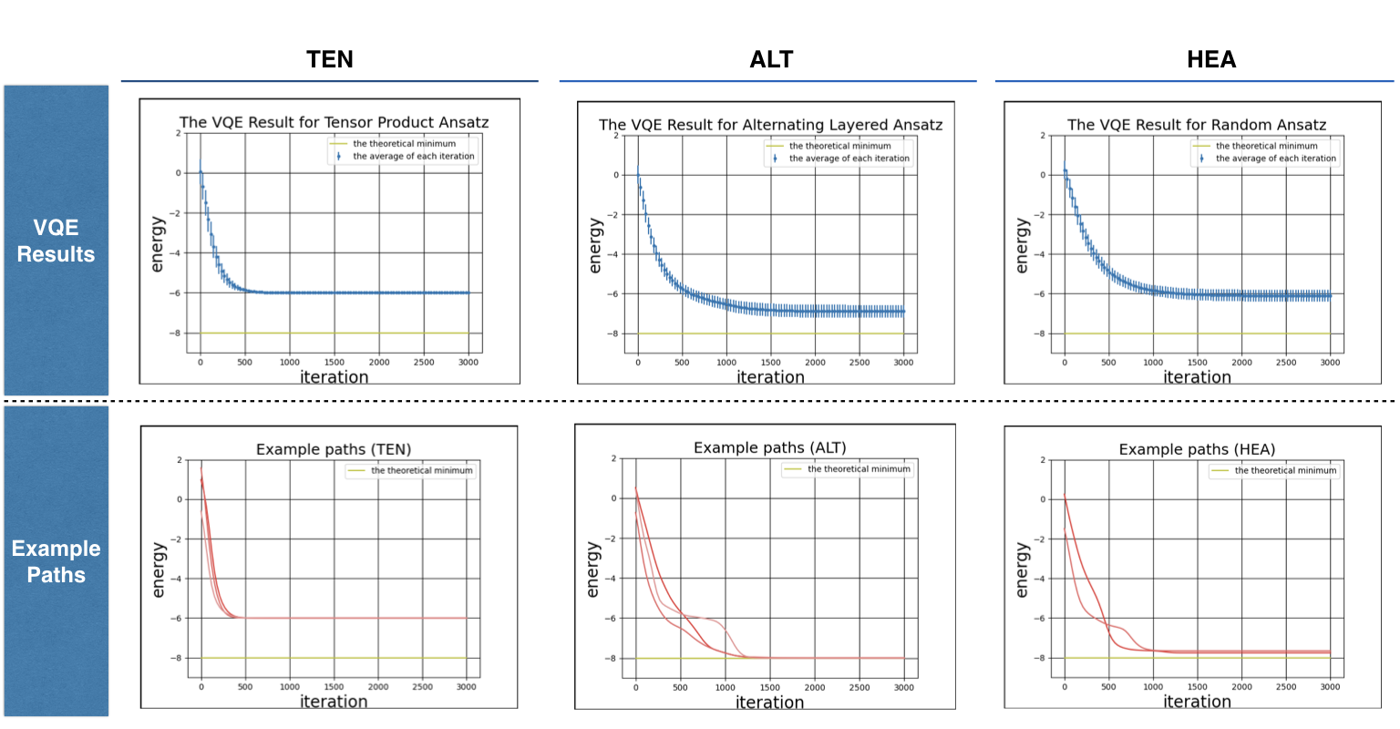
The simulation results are shown in Fig. 5. In the top three subfigures of Fig. 5, the blue lines and the associated error bars represent the average and the standard deviation of \langle{\cal H}\rangle in total 100 trials, respectively. In each trial, the initial parameters of the ansatz are randomly chosen, and the optimization to decrease \langle{\cal H}\rangle in each iteration is performed by using the Adam Optimizer with learning rate 0.0010.001 [18]. The green line shows the theoretical minimum energy (i.e., the ground energy) of {\cal H}. Also the bottom subfigures of Fig. 5 show three trajectories of \langle{\cal H}\rangle (red lines) whose energies at the final iteration step are the smallest three.

The ansatz CTEN3,2,4C_{\rm TEN}^{3,2,4}, which has the least expressibility in the sense of frame potentials and the KL divergence analysis, clearly gives the worst result; its least mean-energy is far above from the ground energy. This is simply because the state generated via CTEN3,2,4C_{\rm TEN}^{3,2,4} cannot represent the ground state for any parameter choice. The result on CHEA4,4C_{\rm HEA}^{4,4} is the second worst, which also does not reach the ground energy as in the case of TEN. Note that increasing the number of parameters does not change this result; that is, we also executed the simulation with CHEA4,6C_{\rm HEA}^{4,6} that has the same number of parameters as CALT3,2,4C_{\rm ALT}^{3,2,4} but did not find a better result than that of CHEA4,4C_{\rm HEA}^{4,4}. On the other hand, CALT3,2,4C_{\rm ALT}^{3,2,4} succeeds in finding the ground state; in fact, 5 of the total 100 trajectories generated via this ALT reach the ground energy. Hence this result implies that, in this example, the expressibility and the trainability coexist in ALT, while the latter is lacking in HEA.

This better trainability of ALT than that of HEA could be explained in terms of the “magnitude” of the gradient vector θ=[/θ1,,/θP]\nabla_{\theta}\langle{\cal H}\rangle=[\partial\langle{\cal H}\rangle/\partial\theta_{1},\ldots,\partial\langle{\cal H}\rangle/\partial\theta_{P}], where PP is the number of parameters. Now care should be taken to define an appropriate magnitude, because the focused ansatzes have different number of parameters. In this work, we regard /θp,(p=1,,P)\partial\langle{\cal H}\rangle/\partial\theta_{p},(p=1,\ldots,P) as random variables and, based on this view, define the magnitude of θ\nabla_{\theta}\langle{\cal H}\rangle as the mean of the absolute value of those random variables:

g(θ)=1Pp=1P|θp|.\displaystyle\|g(\theta)\|=\frac{1}{P}\sum_{p=1}^{P}\left|\frac{\partial\langle{\cal H}\rangle}{\partial\theta_{p}}\right|. (26)

We evaluate the average of the magnitude (26) over sample trajectories, at several values of energy reached through the update of θ\theta. For this purpose, let θC(i)(t)\theta_{C}^{(i)}(t) denote the vector of parameters of a given ansatz CC at the tt-th step (number of iteration) of the ii-th trajectory, and EC(i)(t)=0|UC(θC(i)(t))UC(θC(i)(t))|0E_{C}^{(i)}(t)=\langle 0|U_{C}(\theta_{C}^{(i)}(t))^{\dagger}\mathcal{H}U_{C}(\theta_{C}^{(i)}(t))|0\rangle be the energy at θC(i)(t)\theta_{C}^{(i)}(t). Next, to define the average of g(θC)\|g(\theta_{C})\| over the sample trajectories at the given energy value EE, let tE(i)t_{E}^{(i)} be the smallest integer such that the energy of the ii-th trajectory satisfies EC(i)(tE(i))EE_{C}^{(i)}(t_{E}^{(i)})\leq E; in other words, tE(i)t_{E}^{(i)} represents the number of iteration such that the ii-th trajectory first reaches the value EE. Note that some trajectories may not reach a given value EE for all the repetition of θC\theta_{C}. (For example, as seen above, all trajectories of TEN never reached the value E=7E=-7.) Hence, let E{\cal I}_{E} be the set of index ii such that the ii-th trajectory reaches the value EE at some point of tE(i)t_{E}^{(i)}. We can now define the average of g(θC)\|g(\theta_{C})\| as

g(θC)E=1|E|iEg(θC(i)(tE(i))),\langle\|g(\theta_{C})\|\rangle_{E}=\frac{1}{|{\cal I}_{E}|}\sum_{i\in{\cal I}_{E}}\left\|g(\theta_{C}^{(i)}(t_{E}^{(i)}))\right\|, (27)

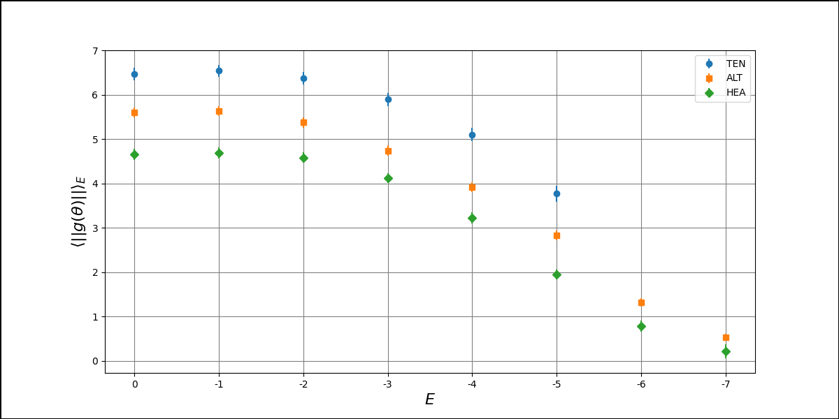
where |E||{\cal I}_{E}| denotes the size of E{\cal I}_{E}. Figure 6 shows Eq. (27) for the specific values of EE (integers from 7-7 to 00) for the three ansatzes CTEN3,2,4C_{\rm TEN}^{3,2,4}, CALT3,2,4C_{\rm ALT}^{3,2,4}, and CHEA4,4C_{\rm HEA}^{4,4}. The standard deviation of the average is indicated by the error bar. For instance, g(θC)E5.6\langle\|g(\theta_{C})\|\rangle_{E}\simeq 5.6 for the case of orange point (i.e., the case of ALT) at E=1E=-1 was calculated with |E|=100|{\cal I}_{E}|=100; actually, all 100 trajectories become lower than E=1E=-1. The figure shows that g(θC)E\langle\|g(\theta_{C})\|\rangle_{E} in ALT is always larger than that in HEA for all EE, and this result is consistent to the theorems given in [8]. Such a larger gradient vector might enable ALT to circumvent possible flat energy landscapes and eventually realize the better trainability than HEA, but further studies are necessary to confirm this observation. Note that TEN has the largest values of g(θC)E\langle\|g(\theta_{C})\|\rangle_{E} when E5E\geq-5, which yet do not lead to the convergence to the global minimum due to the lack of expressibility.
Refer to caption
Figure 5: Top: Energy versus the iteration step in the VQE problem for the Hamiltonian (25), with the ansatz TEN (left), ALT (center), and HEA (right). The blue lines and the associated error bars represent the average and the standard deviation of the mean energies in total 100 trials, respectively; in each trial, the initial parameters of the ansatz are randomly chosen. Optimization to decrease \langle{\cal H}\rangle in each iteration is performed by using Adam Optimizer with learning rate 0.0010.001. Bottom: Three of 100 trajectories for each ansatz TEN (left), ALT (center), and HEA (right), indicated by red lines. The trajectories are chosen such that the energies at the final iteration step are the three smallest values.
Refer to caption
Figure 6: The average and the standard deviation of g(θ)\|g(\theta)\| versus EE. The norm of the gradient is defined as g(θ)=1Pp=1P|θp|\|g(\theta)\|=\frac{1}{P}\sum_{p=1}^{P}\left|\frac{\partial\langle{\mathcal{H}\rangle}}{\partial\theta_{p}}\right|.

5 Conclusion

This paper has examined the expressibility power of the shallow ALT, which was proposed before as a solution to the vanishing gradient problem found in various types of hybrid quantum-classical algorithms. Our conclusion is that, in addition to such a well trainability, shallow ALTs have the expressibility; that is, in the measure of the frame potential and the KL-divergence, those shallow ALTs have almost the same expressibility as HEAs, which are often used in hybrid algorithms but suffer from the vanishing gradient problem. In particular, we have proven that such expressibility holds if the number of entangled qubits in each block is of the order of the logarithm of the number of all resource qubits, which is consistent to the previous result discussing the trainability of ALT. We also provided a case study of VQE problem implying that the ALT enjoys both the expressibility and the trainability.

Although our results are limited to the case =2,3\ell=2,3, we have numerically observed that the ALT acquires even higher expressibility when making \ell bigger. Therefore, we conjecture that the above conclusion still holds for ALT with 4\ell\geq 4. The rigorous proof is left for future work.
Acknowledgement: This work is supported by the MEXT Quantum Leap Flagship Program Grant Number JPMXS0118067285.

Appendix A Proof of Theorems

Notation: For the unitary matrix UaU_{a} corresponding to the entire circuit, we denote the unitary matrix corresponding to the ii-th layer of the circuit to be Ua(i)U_{a}{\left(i\right)} and the unitary matrix corresponding to the jj-th block in the ii-th layer as Ua(i,j)U_{a}{\left(i,j\right)}.

A.1 Proof of Theorem 1

First, because the probability distribution of F=|ψ|ψ|2F=|\langle\psi|\psi^{\prime}\rangle|^{2} with nn-qubits states |ψ|\psi\rangle and |ψ|\psi^{\prime}\rangle taken from the Haar measure is given by PHaar(F)=(2n1)(1F)2n2P_{\mathrm{Haar}}(F)=(2^{n}-1)(1-F)^{2^{n}-2}, the value of Haar(1)(2n)\mathcal{F}^{(1)}_{\rm Haar}(2^{n}) is straightforwardly computed as

Haar(1)(2n)=HaarHaar|ψ|ψ|2𝑑ψdψ=01dFF(2n1)(1F)2n2=12n.\displaystyle\mathcal{F}^{(1)}_{\rm Haar}(2^{n})=\int_{\rm Haar}\int_{\rm Haar}|\langle\psi|\psi^{\prime}\rangle|^{2}d\psi d\psi^{\prime}=\int_{0}^{1}dFF(2^{n}-1)(1-F)^{2^{n}-2}=\frac{1}{2^{n}}. (28)

Next, we provide the proof of (1)(CALT,m,n)=Haar(1)(2n)\mathcal{F}^{(1)}(C_{\rm ALT}^{\ell,m,n})=\mathcal{F}^{(1)}_{\rm Haar}(2^{n}). Given two final states |ϕ=Ua|0|\phi\rangle=U_{a}|0\rangle and |ψ=Ub|0|\psi\rangle=U_{b}|0\rangle generated by CALT,m,nC_{\rm ALT}^{\ell,m,n}, we have

(1)(CALT,m,n)\displaystyle\qquad\mathcal{F}^{(1)}(C_{\rm ALT}^{\ell,m,n}) =1designdUadUb0|UaUb|00|UbUa|0\displaystyle=\int_{\rm 1design}d{U_{a}}d{U_{b}}\langle 0|U_{a}^{\dagger}U_{b}|0\rangle\langle 0|U_{b}^{\dagger}U_{a}|0\rangle
=1design(i=1dUa(i))(i=1dUb(i))\displaystyle=\int_{\rm 1design}\left(\prod_{i=1}^{\ell}dU_{a}{\left(i\right)}\right)\left(\prod_{i=1}^{\ell}dU_{b}{\left(i\right)}\right)
×0|Ua(1)Ua(2)Ua()Ub()Ub(2)Ub(1)|0\displaystyle\qquad\times\langle 0|U_{a}{\left(1\right)}^{\dagger}U_{a}{\left(2\right)}^{\dagger}\cdots U_{a}{\left(\ell\right)}^{\dagger}U_{b}{\left(\ell\right)}\cdots U_{b}{\left(2\right)}U_{b}{\left(1\right)}|0\rangle
×0|Ub(1)Ub(2)Ub()Ua()Ua(2)Ua(1)|0\displaystyle\qquad\times\langle 0|U_{b}{\left(1\right)}^{\dagger}U_{b}{\left(2\right)}^{\dagger}\cdots U_{b}{\left(\ell\right)}^{\dagger}U_{a}{\left(\ell\right)}\cdots U_{a}{\left(2\right)}U_{a}{\left(1\right)}|0\rangle
=1design(i=1(j=1k(i)dUa(i,j)))(i=1(j=1k(i)dUb(i,j)))\displaystyle=\int_{\rm 1design}\left(\prod_{i=1}^{\ell}\left(\prod_{j=1}^{k(i)}dU_{a}{\left(i,j\right)}\right)\right)\left(\prod_{i^{\prime}=1}^{\ell}\left(\prod_{j^{\prime}=1}^{k(i^{\prime})}dU_{b}{\left(i^{\prime},j^{\prime}\right)}\right)\right)
×0|Ua(1)Ua(2)Ua()Ub()Ub(2)Ub(1)|0\displaystyle\qquad\times\langle 0|U_{a}{\left(1\right)}^{\dagger}U_{a}{\left(2\right)}^{\dagger}\cdots U_{a}{\left(\ell\right)}^{\dagger}U_{b}{\left(\ell\right)}\cdots U_{b}{\left(2\right)}U_{b}{\left(1\right)}|0\rangle
×0|Ub(1)Ub(2)Ub()Ua()Ua(2)Ua(1)|0,\displaystyle\qquad\times\langle 0|U_{b}{\left(1\right)}^{\dagger}U_{b}{\left(2\right)}^{\dagger}\cdots U_{b}{\left(\ell\right)}^{\dagger}U_{a}{\left(\ell\right)}\cdots U_{a}{\left(2\right)}U_{a}{\left(1\right)}|0\rangle, (29)

where k(i)k(i) is the number of blocks in the ii-th layer and each 𝑑U\int dU is the average over the ensemble of the unitary matrix UU. Because the distribution of each Ua(i,j)U_{a}{\left(i,j\right)} is 2-design (and is therefore 1-design), we can apply the formula (4) to the integrals with respect to Ua(i,j)U_{a}{\left(i,j\right)}. Actually, by integrating j=1k()dUa(,j)\prod_{j=1}^{k(\ell)}dU_{a}{\left(\ell,j\right)} for all aa in the last line of (A.1), we have

(1)(CALT,m,n)\displaystyle\qquad\mathcal{F}^{(1)}(C_{\rm ALT}^{\ell,m,n}) =1design(i=1(j=1k(i)dUa(i,j)))(i=1(j=1k(i)dUb(i,j)))\displaystyle=\int_{\rm 1design}\left(\prod_{i=1}^{\ell}\left(\prod_{j=1}^{k(i)}dU_{a}{\left(i,j\right)}\right)\right)\left(\prod_{i^{\prime}=1}^{\ell}\left(\prod_{j^{\prime}=1}^{k(i^{\prime})}dU_{b}{\left(i^{\prime},j^{\prime}\right)}\right)\right)
×0|Ua(1)Ua(2)Ua(1)Ua(1)Ua(2)Ua(1)|0\displaystyle\qquad\times\langle 0|U_{a}{\left(1\right)}^{\dagger}U_{a}{\left(2\right)}^{\dagger}\cdots U_{a}{\left(\ell-1\right)}^{\dagger}U_{a}{\left(\ell-1\right)}\cdots U_{a}{\left(2\right)}U_{a}{\left(1\right)}|0\rangle
×0|Ub(1)Ub(2)Ub()Ub()Ub(2)Ub(1)|0\displaystyle\qquad\times\langle 0|U_{b}{\left(1\right)}^{\dagger}U_{b}{\left(2\right)}^{\dagger}\cdots U_{b}{\left(\ell\right)}^{\dagger}U_{b}{\left(\ell\right)}\cdots U_{b}{\left(2\right)}U_{b}{\left(1\right)}|0\rangle
=(12m)1design(i=1L1(α=1k(i)dUaiα))(j=1L(β=1k(i)dUbjβ))×1\displaystyle=\left(\frac{1}{2^{m}}\right)^{\ell}\int_{\rm 1design}\left(\prod_{i=1}^{L-1}\left(\prod_{\alpha=1}^{k(i)}dU_{a}^{i\alpha}\right)\right)\left(\prod_{j=1}^{L}\left(\prod_{\beta=1}^{k(i^{\prime})}dU_{b}^{j\beta}\right)\right)\times 1
=12n=Haar(1)(2n).\displaystyle=\frac{1}{2^{n}}=\mathcal{F}^{(1)}_{\rm Haar}(2^{n}). (30)

The other equality in Eq. (7) can be proved in the same manner.

A.2 Proof of Theorem 2

Similar to the first frame potential, the value of Haar(1)(2n)\mathcal{F}^{(1)}_{\rm Haar}(2^{n}) is straightforwardly computed as

Haar(2)(2n)=01dFF2(2n1)(1F)2n2=12n1(2n+1).\displaystyle\mathcal{F}^{(2)}_{\rm Haar}(2^{n})=\int_{0}^{1}dFF^{2}(2^{n}-1)(1-F)^{2^{n}-2}=\frac{1}{2^{n-1}(2^{n}+1)}. (31)

Next, we compute (2)(CTEN,m,n)\mathcal{F}^{(2)}(C_{\rm TEN}^{\ell,m,n}). Given two final states |ϕ=Ua|0|\phi\rangle=U_{a}|0\rangle and |ψ=Ub|0|\psi\rangle=U_{b}|0\rangle, it is computed as

(2)(CTEN,m,n)\displaystyle\mathcal{F}^{(2)}(C_{\rm TEN}^{\ell,m,n}) =2design(i=1dUa(i,1)dUb(i,1))|0|Ua(1,1)Ua(2,1)Ua(,1)Ub(,1)Ub(2,1)Ub(1,1)|0|4\displaystyle=\int_{\rm 2design}\left(\prod_{i=1}^{\ell}d{U_{a}{\left(i,1\right)}}d{U_{b}{\left(i,1\right)}}\right)|\langle 0|U_{a}{\left(1,1\right)}^{\dagger}U_{a}{\left(2,1\right)}^{\dagger}\cdots U_{a}{\left(\ell,1\right)}^{\dagger}U_{b}{\left(\ell,1\right)}\cdots U_{b}{\left(2,1\right)}U_{b}{\left(1,1\right)}|0\rangle|^{4}
×2design(i=1dUa(i,2)dUb(i,2))|0|Ua(1,2)Ua(2,2)Ua(,2)Ub(,2)Ub(2,2)Ub(1,2)|0|4\displaystyle\times\int_{\rm 2design}\left(\prod_{i=1}^{\ell}d{U_{a}{\left(i,2\right)}}d{U_{b}{\left(i,2\right)}}\right)|\langle 0|U_{a}{\left(1,2\right)}^{\dagger}U_{a}{\left(2,2\right)}^{\dagger}\cdots U_{a}{\left(\ell,2\right)}^{\dagger}U_{b}{\left(\ell,2\right)}\cdots U_{b}{\left(2,2\right)}U_{b}{\left(1,2\right)}|0\rangle|^{4}
××2design(i=1dUa(i,nm)dUb(i,nm))\displaystyle\times\cdots\times\int_{\rm 2design}\left(\prod_{i=1}^{\ell}d{U_{a}{\left(i,\frac{n}{m}\right)}}d{U_{b}{\left(i,\frac{n}{m}\right)}}\right)
×|0|Ua(,1)Ua(,2)Ua(,)Ub(,)Ub(,2)Ub(,1)|0|4\displaystyle\qquad\qquad\times|\langle 0|U_{a}{\left(\ell,1\right)}^{\dagger}U_{a}{\left(\ell,2\right)}^{\dagger}\cdots U_{a}{\left(\ell,\ell\right)}^{\dagger}U_{b}{\left(\ell,\ell\right)}\cdots U_{b}{\left(\ell,2\right)}U_{b}{\left(\ell,1\right)}|0\rangle|^{4}
=(1(2m+1)2m1)nm=2nm12n+1(2m+1)nmHaar(2)(2n).\displaystyle=\left(\frac{1}{(2^{m}+1)2^{m-1}}\right)^{\frac{n}{m}}=2^{\frac{n}{m}-1}\cdot\frac{2^{n}+1}{(2^{m}+1)^{\frac{n}{m}}}\mathcal{F}^{(2)}_{\rm Haar}(2^{n}). (32)

A.3 Proof of Theorem 3

Here we only show the computation of (2)(CALT3,m,n)\mathcal{F}^{(2)}(C_{\rm ALT}^{3,m,n}). The computation of (2)(CALT2,m,n)\mathcal{F}^{(2)}(C_{\rm ALT}^{2,m,n}) can be done in a similar manner. The second frame potential can be expressed as follows:

(2)(CALT3,m,n)\displaystyle\mathcal{F}^{(2)}(C_{\rm ALT}^{3,m,n}) =dUa(1)dUa(2)dUa(3)dUb(1)dUb(2)dUb(3)|0|Ua(1)Ua(2)Ua(3)Ub(3)Ub(2)Ub(1)|0|4\displaystyle=\int dU_{a}{\left(1\right)}dU_{a}{\left(2\right)}dU_{a}{\left(3\right)}dU_{b}{\left(1\right)}dU_{b}{\left(2\right)}dU_{b}{\left(3\right)}~|\langle 0|U_{a}{\left(1\right)}^{\dagger}U_{a}{\left(2\right)}^{\dagger}U_{a}{\left(3\right)}^{\dagger}U_{b}{\left(3\right)}U_{b}{\left(2\right)}U_{b}{\left(1\right)}|0\rangle|^{4}
=2design(i=13j=1k(i)dUa(i,j))(i=13j=1k(i)dUb(i,j))\displaystyle=\int_{\rm 2design}\left(\prod_{i=1}^{3}\prod_{j=1}^{k(i)}dU_{a}{\left(i,j\right)}\right)\left(\prod_{i^{\prime}=1}^{3}\prod_{j^{\prime}=1}^{k(i)}dU_{b}{\left(i^{\prime},j^{\prime}\right)}\right)
×|0|Ua(1,1)Ua(1,2)Ua(1,n/m)Ua(2,1)Ua(2,2)Ua(2,n/m+1)\displaystyle\qquad\times|\langle 0|U_{a}{\left(1,1\right)}^{\dagger}U_{a}{\left(1,2\right)}^{\dagger}\cdots U_{a}{\left(1,n/m\right)}^{\dagger}U_{a}{\left(2,1\right)}^{\dagger}U_{a}{\left(2,2\right)}^{\dagger}\cdots U_{a}{\left(2,n/m+1\right)}^{\dagger}
×Ua(3,1)Ua(3,2)Ua(3,n/m)Ub(3,n/m)Ub(3,2)Ub(3,1)\displaystyle\qquad\qquad\times U_{a}{\left(3,1\right)}^{\dagger}U_{a}{\left(3,2\right)}^{\dagger}\cdots U_{a}{\left(3,n/m\right)}^{\dagger}U_{b}{\left(3,n/m\right)}\cdots U_{b}{\left(3,2\right)}U_{b}{\left(3,1\right)}
×Ub(2,n/m+1)Ub(2,2)Ub(2,1)Ub(1,n/m)Ub(1,2)Ub(1,1)|0|4.\displaystyle\qquad\qquad\qquad\times U_{b}{\left(2,n/m+1\right)}\cdots U_{b}{\left(2,2\right)}U_{b}{\left(2,1\right)}U_{b}{\left(1,n/m\right)}\cdots U_{b}{\left(1,2\right)}U_{b}{\left(1,1\right)}|0\rangle|^{4}.

Recall that k(i)k(i) denotes the number of blocks in ii-th layer; k(i)=n/mk(i)=n/m for i=1,3i=1,3 and k(i)=n/m+1k(i)=n/m+1 for i=2i=2. We can get the final formula in the theorem by integrating only the unitary matrices in the first layer and the third layer. Executing integrals 2designj=1n/mdUa(,j)\int_{\rm 2design}\prod_{j=1}^{n/m}dU_{a}{\left(\ell,j\right)} and 2designj=1n/mdUb(,j)\int_{\rm 2design}\prod_{j^{\prime}=1}^{n/m}dU_{b}{\left(\ell,j^{\prime}\right)} for =1,3\ell=1,3, we have

(2)(CALT3,m,n)\displaystyle\mathcal{F}^{(2)}(C_{\rm ALT}^{3,m,n}) =2design(j=1n/m+1dUa(2,j))(j=1n/m+1dUb(2,j))\displaystyle=\int_{\rm 2design}\left(\prod_{j=1}^{n/m+1}dU_{a}{\left(2,j\right)}\right)\left(\prod_{j^{\prime}=1}^{n/m+1}dU_{b}{\left(2,j^{\prime}\right)}\right)
k11a=14k12a=14k1nma=14k31a=14k32a=14k3nma=14k11b=14k12b=14k1nmb=14\displaystyle\sum_{k_{11}^{a}=1}^{4}\sum_{k_{12}^{a}=1}^{4}\cdots\sum_{k_{1\frac{n}{m}}^{a}=1}^{4}\sum_{k_{31}^{a}=1}^{4}\sum_{k_{32}^{a}=1}^{4}\cdots\sum_{k_{3\frac{n}{m}}^{a}=1}^{4}\sum_{k_{11}^{b}=1}^{4}\sum_{k_{12}^{b}=1}^{4}\cdots\sum_{k_{1\frac{n}{m}}^{b}=1}^{4}
λk11a(m)λk12a(m)λk1nm1a(m)λk1nma(m)λk31a(m)λk32a(m)λk3nm1a(m)λk3nma(m)λk11b(m)λk12b(m)λk1nm1b(m)λk1nmb(m)\displaystyle\lambda_{k_{11}^{a}}^{(m)}\lambda_{k_{12}^{a}}^{(m)}\cdots\lambda_{k_{1\frac{n}{m}-1}^{a}}^{(m)}\lambda_{k_{1\frac{n}{m}}^{a}}^{(m)}\lambda_{k_{31}^{a}}^{(m)}\lambda_{k_{32}^{a}}^{(m)}\cdots\lambda_{k_{3\frac{n}{m}-1}^{a}}^{(m)}\lambda_{k_{3\frac{n}{m}}^{a}}^{(m)}\lambda_{k_{11}^{b}}^{(m)}\lambda_{k_{12}^{b}}^{(m)}\cdots\lambda_{k_{1\frac{n}{m}-1}^{b}}^{(m)}\lambda_{k_{1\frac{n}{m}}^{b}}^{(m)}
×Δ(k11a,k31a,k11b)(Ua(2,1),Ub(2,1))×Δ(k11a,k31a,k11b,k12a,k32a,k12b)(Ua(2,2),Ub(2,2))\displaystyle\times\Delta^{(k_{11}^{a},k_{31}^{a},k_{11}^{b})}\left(U_{a}{\left(2,1\right)},U_{b}{\left(2,1\right)}\right)\times\Delta^{\left(k_{11}^{a},k_{31}^{a},k_{11}^{b},k_{12}^{a},k_{32}^{a},k_{12}^{b}\right)}(U_{a}{\left(2,2\right)},U_{b}{\left(2,2\right)})
×Δ(k12a,k32a,k12b,k13a,k33a,k13b)(Ua(2,3),Ub(2,3))×\displaystyle\times\Delta^{\left(k_{12}^{a},k_{32}^{a},k_{12}^{b},k_{13}^{a},k_{33}^{a},k_{13}^{b}\right)}(U_{a}{\left(2,3\right)},U_{b}{\left(2,3\right)})\times\cdots
×Δ(k1nm1a,k3nm1a,k1nm1b,k1nma,k3nma,k1nmb)(Ua(2,nm),Ub(2,nm))\displaystyle\times\Delta^{\left(k_{1\frac{n}{m}-1}^{a},k_{3\frac{n}{m}-1}^{a},k_{1\frac{n}{m}-1}^{b},k_{1\frac{n}{m}}^{a},k_{3\frac{n}{m}}^{a},k_{1\frac{n}{m}}^{b}\right)}(U_{a}{\left(2,\frac{n}{m}\right)},U_{b}{\left(2,\frac{n}{m}\right)})
×Δ(k1nma,k3nma,k1nmb)(Ua(2,nm+1),Ub(2,nm+1))\displaystyle\times\Delta^{(k_{1\frac{n}{m}}^{a},k_{3\frac{n}{m}}^{a},k_{1\frac{n}{m}}^{b})}\left(U_{a}{\left(2,\frac{n}{m}+1\right)},U_{b}{\left(2,\frac{n}{m}+1\right)}\right)
=k11a=14k12a=14k1nma=14k31a=14k32a=14k3,nma=14k11b=14k12b=14k1nmb=14\displaystyle=\sum_{k_{11}^{a}=1}^{4}\sum_{k_{12}^{a}=1}^{4}\cdots\sum_{k_{1\frac{n}{m}}^{a}=1}^{4}\sum_{k_{31}^{a}=1}^{4}\sum_{k_{32}^{a}=1}^{4}\cdots\sum_{k_{3,\frac{n}{m}}^{a}=1}^{4}\sum_{k_{11}^{b}=1}^{4}\sum_{k_{12}^{b}=1}^{4}\cdots\sum_{k_{1\frac{n}{m}}^{b}=1}^{4}
2designdUa(2,1)dUb(2,1)λk11a(m)λk31a(m)λk11b(m)Δ(k11a,k31a,k11b)(Ua(2,1),Ub(2,1))\displaystyle\int_{\rm 2design}dU_{a}{\left(2,1\right)}dU_{b}{\left(2,1\right)}\sqrt{\lambda_{k_{11}^{a}}^{(m)}\lambda_{k_{31}^{a}}^{(m)}\lambda_{k_{11}^{b}}^{(m)}}\Delta^{(k_{11}^{a},k_{31}^{a},k_{11}^{b})}\left(U_{a}{\left(2,1\right)},U_{b}{\left(2,1\right)}\right)
×2designdUa(2,2)dUb(2,b)λk11a(m)λk31a(m)λk11b(m)λk12a(m)λk32a(m)λk12b(m)Δ(k11a,k31a,k11b,k12a,k32a,k12b)(Ua(2,2),Ub(2,2))\displaystyle\times\int_{\rm 2design}dU_{a}{\left(2,2\right)}dU_{b}{\left(2,b\right)}\sqrt{\lambda_{k_{11}^{a}}^{(m)}\lambda_{k_{31}^{a}}^{(m)}\lambda_{k_{11}^{b}}^{(m)}}\sqrt{\lambda_{k_{12}^{a}}^{(m)}\lambda_{k_{32}^{a}}^{(m)}\lambda_{k_{12}^{b}}^{(m)}}\Delta^{\left(k_{11}^{a},k_{31}^{a},k_{11}^{b},k_{12}^{a},k_{32}^{a},k_{12}^{b}\right)}(U_{a}{\left(2,2\right)},U_{b}{\left(2,2\right)})
×2designdUa(2,3)dUb(2,3)λk12a(m)λk32a(m)λk12b(m)λk13a(m)λk33a(m)λk13b(m)Δ(k12a,k32a,k12b,k13a,k33a,k13b)(Ua(2,3),Ub(2,3))\displaystyle\times\int_{\rm 2design}dU_{a}{\left(2,3\right)}dU_{b}{\left(2,3\right)}\sqrt{\lambda_{k_{12}^{a}}^{(m)}\lambda_{k_{32}^{a}}^{(m)}\lambda_{k_{12}^{b}}^{(m)}}\sqrt{\lambda_{k_{13}^{a}}^{(m)}\lambda_{k_{33}^{a}}^{(m)}\lambda_{k_{13}^{b}}^{(m)}}\Delta^{\left(k_{12}^{a},k_{32}^{a},k_{12}^{b},k_{13}^{a},k_{33}^{a},k_{13}^{b}\right)}(U_{a}{\left(2,3\right)},U_{b}{\left(2,3\right)})
××2designdUa(2,nm)dUb(2,nm)λk1nm1a(m)λk3nm1a(m)λk1nm1b(m)λk1nma(m)λk3nma(m)λk1nmb(m)\displaystyle\times\cdots\times\int_{\rm 2design}dU_{a}{\left(2,\frac{n}{m}\right)}dU_{b}{\left(2,\frac{n}{m}\right)}\sqrt{\lambda_{k_{1\frac{n}{m}-1}^{a}}^{(m)}\lambda_{k_{3\frac{n}{m}-1}^{a}}^{(m)}\lambda_{k_{1\frac{n}{m}-1}^{b}}^{(m)}}\sqrt{\lambda_{k_{1\frac{n}{m}}^{a}}^{(m)}\lambda_{k_{3\frac{n}{m}}^{a}}^{(m)}\lambda_{k_{1\frac{n}{m}}^{b}}^{(m)}}
×Δ(k1nm1a,k3nm1a,k1nm1b,k1nma,k3nma,k1nmb)(Ua(2,nm),Ub(2,nm))\displaystyle\qquad\qquad\times\Delta^{\left(k_{1\frac{n}{m}-1}^{a},k_{3\frac{n}{m}-1}^{a},k_{1\frac{n}{m}-1}^{b},k_{1\frac{n}{m}}^{a},k_{3\frac{n}{m}}^{a},k_{1\frac{n}{m}}^{b}\right)}(U_{a}{\left(2,\frac{n}{m}\right)},U_{b}{\left(2,\frac{n}{m}\right)})
×2designdUa(2,nm+1)dUb(2,nm+1)λk1nma(m)λk3nma(m)λk1nmb(m)\displaystyle\times\int_{\rm 2design}dU_{a}{\left(2,\frac{n}{m}+1\right)}dU_{b}{\left(2,\frac{n}{m}+1\right)}\sqrt{\lambda_{k_{1\frac{n}{m}}^{a}}^{(m)}\lambda_{k_{3\frac{n}{m}}^{a}}^{(m)}\lambda_{k_{1\frac{n}{m}}^{b}}^{(m)}}
×Δ(k1nma,k3nma,k1nmb)(Ua(2,nm+1),Ub(2,nm+1))\displaystyle\qquad\qquad\times\Delta^{(k_{1\frac{n}{m}}^{a},k_{3\frac{n}{m}}^{a},k_{1\frac{n}{m}}^{b})}\left(U_{a}{\left(2,\frac{n}{m}+1\right)},U_{b}{\left(2,\frac{n}{m}+1\right)}\right)
=𝐚(3,m)TB(3,m)nm1𝐚(3,m),\displaystyle={\bf a}(3,m)^{\rm T}B(3,m)^{\frac{n}{m}-1}{\bf a}(3,m), (33)

where we use definitions: (13), (14), (3.1), and (3.1). For the purpose of exemplifying the computation in the first equality of (A.3), we show the computation when n/m=2n/m=2 in the following. When n/m=2n/m=2, the second frame potential can be computed as follows:

(2)(CALT3,n,m)\displaystyle\mathcal{F}^{(2)}(C_{\rm ALT}^{3,n,m}) =2designdUa(1,1)dUa(1,2)dUa(2,1)dUa(2,2)dUa(2,3)dUa(3,1)dUa(3,2)\displaystyle=\int_{\rm 2design}dU_{a}(1,1)dU_{a}(1,2)dU_{a}(2,1)dU_{a}(2,2)dU_{a}(2,3)dU_{a}(3,1)dU_{a}(3,2)
dUb(1,1)dUb(1,2)dUb(2,1)dUb(2,2)dUb(2,3)dUb(3,1)dUb(3,2)\displaystyle\qquad\qquad\qquad dU_{b}(1,1)dU_{b}(1,2)dU_{b}(2,1)dU_{b}(2,2)dU_{b}(2,3)dU_{b}(3,1)dU_{b}(3,2)
|0|Ua(1,1)Ua(1,2)Ua(2,1)Ua(2,2)Ua(2,3)Ua(3,1)Ua(3,2)\displaystyle\qquad\qquad\qquad|\langle 0|U^{\dagger}_{a}(1,1)U^{\dagger}_{a}(1,2)U^{\dagger}_{a}(2,1)U^{\dagger}_{a}(2,2)U^{\dagger}_{a}(2,3)U^{\dagger}_{a}(3,1)U^{\dagger}_{a}(3,2)
Ub(3,1)Ub(3,2)Ub(2,1)Ub(2,2)Ub(2,3)Ub(1,1)Ub(1,2)|0|4\displaystyle\qquad\qquad\qquad\qquad U_{b}(3,1)U_{b}(3,2)U_{b}(2,1)U_{b}(2,2)U_{b}(2,3)U_{b}(1,1)U_{b}(1,2)|0\rangle|^{4}
=2designdUa(1,1)dUa(1,2)dUa(2,1)dUa(2,2)dUa(2,3)dUa(3,1)dUa(3,2)\displaystyle=\int_{\rm 2design}dU_{a}(1,1)dU_{a}(1,2)dU_{a}(2,1)dU_{a}(2,2)dU_{a}(2,3)dU_{a}(3,1)dU_{a}(3,2)
dUb(1,1)dUb(1,2)dUb(2,1)dUb(2,2)dUb(2,3)dUb(3,1)dUb(3,2)\displaystyle\qquad\qquad\qquad dU_{b}(1,1)dU_{b}(1,2)dU_{b}(2,1)dU_{b}(2,2)dU_{b}(2,3)dU_{b}(3,1)dU_{b}(3,2)
𝐢,𝐣,𝐤,𝐥,𝐩(Ua(1,1)i10i20Ua(1,2)i30i40Ua(2,1)j1i1Ua(2,2)j2i2j3i3Ua(2,3)j4i4Ua(3,1)k1j1k2j2Ua(3,2)k3j3k4j4CLOSE\displaystyle\qquad\qquad\sum_{\bf i,j,k,l,p}\left(U_{a}^{\ast}(1,1)_{i_{1}0}^{i_{2}0}U_{a}^{\ast}(1,2)_{i_{3}0}^{i_{4}0}U_{a}^{\ast}(2,1)_{j_{1}i_{1}}U_{a}^{\ast}(2,2)_{j_{2}i_{2}}^{j_{3}i_{3}}U_{a}^{\ast}(2,3)_{j_{4}i_{4}}U_{a}^{\ast}(3,1)_{k_{1}j_{1}}^{k_{2}j_{2}}U_{a}^{\ast}(3,2)_{k_{3}j_{3}}^{k_{4}j_{4}}\right.
Ub(3,1)k1l1k2l2Ub(3,2)k3l3k4l4Ub(2,1)l1p1Ub(2,2)l2p2l3p3Ub(2,3)l4p4Ub(1,1)p10p20Ub(1,2)p30p40)×\displaystyle\qquad\qquad\qquad\left.U_{b}(3,1)_{k_{1}l_{1}}^{k_{2}l_{2}}U_{b}(3,2)_{k_{3}l_{3}}^{k_{4}l_{4}}U_{b}(2,1)_{l_{1}p_{1}}U_{b}(2,2)_{l_{2}p_{2}}^{l_{3}p_{3}}U_{b}(2,3)_{l_{4}p_{4}}U_{b}(1,1)_{p_{1}0}^{p_{2}0}U_{b}(1,2)_{p_{3}0}^{p_{4}0}\right)\times
𝐪,𝐫,𝐬,𝐭,𝐮(Ub(1,1)q10q20Ub(1,2)q30q40Ub(2,1)r1q1Ub(2,2)r2q2r3q3Ub(2,3)r4q4Ub(3,1)s1r1s2r2Ub(3,2)s3r3s4r4CLOSE\displaystyle\qquad\qquad\sum_{\bf q,r,s,t,u}\left(U_{b}^{\ast}(1,1)_{q_{1}0}^{q_{2}0}U_{b}^{\ast}(1,2)_{q_{3}0}^{q_{4}0}U_{b}^{\ast}(2,1)_{r_{1}q_{1}}U_{b}^{\ast}(2,2)_{r_{2}q_{2}}^{r_{3}q_{3}}U_{b}^{\ast}(2,3)_{r_{4}q_{4}}U_{b}^{\ast}(3,1)_{s_{1}r_{1}}^{s_{2}r_{2}}U_{b}^{\ast}(3,2)_{s_{3}r_{3}}^{s_{4}r_{4}}\right.
Ua(3,1)s1t1s2t2Ua(3,2)s3t3s4t4Ua(2,1)t1u1Ua(2,2)t2u2t3u3Ua(2,3)t4u4Ua(1,1)u10u20Ua(1,2)u30u40)×\displaystyle\qquad\qquad\qquad\left.U_{a}(3,1)_{s_{1}t_{1}}^{s_{2}t_{2}}U_{a}(3,2)_{s_{3}t_{3}}^{s_{4}t_{4}}U_{a}(2,1)_{t_{1}u_{1}}U_{a}(2,2)_{t_{2}u_{2}}^{t_{3}u_{3}}U_{a}(2,3)_{t_{4}u_{4}}U_{a}(1,1)_{u_{1}0}^{u_{2}0}U_{a}(1,2)_{u_{3}0}^{u_{4}0}\right)\times
𝐢,𝐣,𝐤,𝐥,𝐩(Ua(1,1)i10i20Ua(1,2)i30i40Ua(2,1)j1i1Ua(2,2)j2i2j3i3Ua(2,3)j4i4Ua(3,1)k1j1k2j2Ua(3,2)k3j3k4j4CLOSE\displaystyle\qquad\qquad\sum_{\bf i^{\prime},j^{\prime},k^{\prime},l^{\prime},p^{\prime}}\left(U_{a}^{\ast}(1,1)_{i^{\prime}_{1}0}^{i^{\prime}_{2}0}U_{a}^{\ast}(1,2)_{i^{\prime}_{3}0}^{i^{\prime}_{4}0}U_{a}^{\ast}(2,1)_{j^{\prime}_{1}i^{\prime}_{1}}U_{a}^{\ast}(2,2)_{j^{\prime}_{2}i^{\prime}_{2}}^{j^{\prime}_{3}i^{\prime}_{3}}U_{a}^{\ast}(2,3)_{j^{\prime}_{4}i^{\prime}_{4}}U_{a}^{\ast}(3,1)_{k^{\prime}_{1}j^{\prime}_{1}}^{k^{\prime}_{2}j^{\prime}_{2}}U_{a}^{\ast}(3,2)_{k^{\prime}_{3}j^{\prime}_{3}}^{k^{\prime}_{4}j^{\prime}_{4}}\right.
Ub(3,1)k1l1k2l2Ub(3,2)k3l3k4l4Ub(2,1)l1p1Ub(2,2)l2p2l3p3Ub(2,3)l4p4Ub(1,1)p10p20Ub(1,2)p30p40)×\displaystyle\qquad\qquad\qquad\left.U_{b}(3,1)_{k^{\prime}_{1}l^{\prime}_{1}}^{k^{\prime}_{2}l^{\prime}_{2}}U_{b}(3,2)_{k^{\prime}_{3}l^{\prime}_{3}}^{k^{\prime}_{4}l^{\prime}_{4}}U_{b}(2,1)_{l^{\prime}_{1}p^{\prime}_{1}}U_{b}(2,2)_{l^{\prime}_{2}p^{\prime}_{2}}^{l^{\prime}_{3}p^{\prime}_{3}}U_{b}(2,3)_{l^{\prime}_{4}p^{\prime}_{4}}U_{b}(1,1)_{p^{\prime}_{1}0}^{p^{\prime}_{2}0}U_{b}(1,2)_{p^{\prime}_{3}0}^{p^{\prime}_{4}0}\right)\times
𝐪,𝐫,𝐬,𝐭,𝐮(Ub(1,1)q10q20Ub(1,2)q30q40Ub(2,1)r1q1Ub(2,2)r2q2r3q3Ub(2,3)r4q4Ub(3,1)s1r1s2r2Ub(3,2)s3r3s4r4CLOSE\displaystyle\qquad\qquad\sum_{\bf q^{\prime},r^{\prime},s^{\prime},t^{\prime},u^{\prime}}\left(U_{b}^{\ast}(1,1)_{q^{\prime}_{1}0}^{q^{\prime}_{2}0}U_{b}^{\ast}(1,2)_{q^{\prime}_{3}0}^{q^{\prime}_{4}0}U_{b}^{\ast}(2,1)_{r^{\prime}_{1}q^{\prime}_{1}}U_{b}^{\ast}(2,2)_{r^{\prime}_{2}q^{\prime}_{2}}^{r^{\prime}_{3}q^{\prime}_{3}}U_{b}^{\ast}(2,3)_{r^{\prime}_{4}q^{\prime}_{4}}U_{b}^{\ast}(3,1)_{s^{\prime}_{1}r^{\prime}_{1}}^{s^{\prime}_{2}r^{\prime}_{2}}U_{b}^{\ast}(3,2)_{s^{\prime}_{3}r^{\prime}_{3}}^{s^{\prime}_{4}r^{\prime}_{4}}\right.
OPENUa(3,1)s1t1s2t2Ua(3,2)s3t3s4t4Ua(2,1)t1u1Ua(2,2)t2u2t3u3Ua(2,3)t4u4Ua(1,1)u10u20Ua(1,2)u30u40)\displaystyle\qquad\qquad\qquad\left.U_{a}(3,1)_{s^{\prime}_{1}t^{\prime}_{1}}^{s^{\prime}_{2}t^{\prime}_{2}}U_{a}(3,2)_{s^{\prime}_{3}t^{\prime}_{3}}^{s^{\prime}_{4}t^{\prime}_{4}}U_{a}(2,1)_{t^{\prime}_{1}u^{\prime}_{1}}U_{a}(2,2)_{t^{\prime}_{2}u^{\prime}_{2}}^{t^{\prime}_{3}u^{\prime}_{3}}U_{a}(2,3)_{t^{\prime}_{4}u^{\prime}_{4}}U_{a}(1,1)_{u^{\prime}_{1}0}^{u^{\prime}_{2}0}U_{a}(1,2)_{u^{\prime}_{3}0}^{u^{\prime}_{4}0}\right) (34)

where the bold symbols in the bottom the summation denote the multiple indices, e.g., 𝐢=i1,i2,i3,i4{\bf i}=i_{1},i_{2},i_{3},i_{4}. For the integrals Ua(1,1),Ub(1,1),Ua(1,2),Ub(1,2)U_{a}(1,1),U_{b}(1,1),U_{a}(1,2),U_{b}(1,2),

2designdUa(1,1)Ua(1,1)u10u20Ua(1,1)u10u20Ua(1,1)i10i20Ua(1,1)i10i20\displaystyle\int_{\rm 2design}dU_{a}(1,1)U_{a}(1,1)_{u_{1}0}^{u_{2}0}U_{a}(1,1)_{u^{\prime}_{1}0}^{u^{\prime}_{2}0}U_{a}^{\ast}(1,1)_{i_{1}0}^{i_{2}0}U_{a}^{\ast}(1,1)_{i^{\prime}_{1}0}^{i^{\prime}_{2}0} =k11a=14λk11a(m)Δu10u10i10i10k11aΔu20u20i20i20k11a,\displaystyle=\sum_{k_{11}^{a}=1}^{4}\lambda_{k_{11}^{a}}^{(m)}\Delta^{k_{11}^{a}}_{u_{1}0u^{\prime}_{1}0i_{1}0i^{\prime}_{1}0}\Delta^{k_{11}^{a}}_{u_{2}0u^{\prime}_{2}0i_{2}0i^{\prime}_{2}0}, (35)
2designdUb(1,1)Ub(1,1)p10p20Ub(1,1)p10p20Ub(1,1)q10q20Ub(1,1)q10q20\displaystyle\int_{\rm 2design}dU_{b}(1,1)U_{b}(1,1)_{p_{1}0}^{p_{2}0}U_{b}(1,1)_{p^{\prime}_{1}0}^{p^{\prime}_{2}0}U_{b}^{\ast}(1,1)_{q_{1}0}^{q_{2}0}U_{b}^{\ast}(1,1)_{q^{\prime}_{1}0}^{q^{\prime}_{2}0} =k11b=14λk11b(m)Δp10p10q10q10k11bΔp20p20q20q20k11b,\displaystyle=\sum_{k_{11}^{b}=1}^{4}\lambda_{k_{11}^{b}}^{(m)}\Delta^{k_{11}^{b}}_{p_{1}0p^{\prime}_{1}0q_{1}0q^{\prime}_{1}0}\Delta^{k_{11}^{b}}_{p_{2}0p^{\prime}_{2}0q_{2}0q^{\prime}_{2}0}, (36)
2designdUa(1,2)Ua(1,2)u30u40Ua(1,2)u30u40Ua(1,2)i30i40Ua(1,2)i30i40\displaystyle\int_{\rm 2design}dU_{a}(1,2)U_{a}(1,2)_{u_{3}0}^{u_{4}0}U_{a}(1,2)_{u^{\prime}_{3}0}^{u^{\prime}_{4}0}U_{a}^{\ast}(1,2)_{i_{3}0}^{i_{4}0}U_{a}^{\ast}(1,2)_{i^{\prime}_{3}0}^{i^{\prime}_{4}0} =k12a=14λk12a(m)Δu30u30i30i30k12aΔu40u40i40i40k12a,\displaystyle=\sum_{k_{12}^{a}=1}^{4}\lambda_{k_{12}^{a}}^{(m)}\Delta^{k_{12}^{a}}_{u_{3}0u^{\prime}_{3}0i_{3}0i^{\prime}_{3}0}\Delta^{k_{12}^{a}}_{u_{4}0u^{\prime}_{4}0i_{4}0i^{\prime}_{4}0}, (37)
2designdUb(1,2)Ub(1,2)p30p40Ub(1,2)p30p40Ub(1,2)q30q40Ub(1,2)q30q40\displaystyle\int_{\rm 2design}dU_{b}(1,2)U_{b}(1,2)_{p_{3}0}^{p_{4}0}U_{b}(1,2)_{p^{\prime}_{3}0}^{p^{\prime}_{4}0}U_{b}^{\ast}(1,2)_{q_{3}0}^{q_{4}0}U_{b}^{\ast}(1,2)_{q^{\prime}_{3}0}^{q^{\prime}_{4}0} =k12b=14λk12b(m)Δp30p30q30q30k12bΔp40p40q40q40k12b\displaystyle=\sum_{k_{12}^{b}=1}^{4}\lambda_{k_{12}^{b}}^{(m)}\Delta^{k_{12}^{b}}_{p_{3}0p^{\prime}_{3}0q_{3}0q^{\prime}_{3}0}\Delta^{k_{12}^{b}}_{p_{4}0p^{\prime}_{4}0q_{4}0q^{\prime}_{4}0} (38)

hold. For the integrals Ua(3,1),Ub(3,1),Ua(3,2),Ub(3,2)U_{a}(3,1),U_{b}(3,1),U_{a}(3,2),U_{b}(3,2),

2designdUa(3,1)dUb(3,1)\displaystyle\int_{\rm 2design}dU_{a}(3,1)dU_{b}(3,1)
k1,k2s1,s2k1,k2s1,s2Ua(3,1)k1j1k2j2Ub(3,1)k1l1k2l2Ub(3,1)s1r1s2r2Ua(3,1)s1t1s2t2Ua(3,1)k1j1k2j2Ub(3,1)k1l1k2l2Ub(3,1)s1r1s2r2Ua(3,1)s1t1s2t2\displaystyle\qquad\sum_{\begin{subarray}{c}k_{1},k_{2}\\ s_{1},s_{2}\\ \end{subarray}}\sum_{\begin{subarray}{c}k^{\prime}_{1},k^{\prime}_{2}\\ s^{\prime}_{1},s^{\prime}_{2}\\ \end{subarray}}U^{\ast}_{a}(3,1)^{k_{2}j_{2}}_{k_{1}j_{1}}U_{b}(3,1)_{k_{1}l_{1}}^{k_{2}l_{2}}U^{\ast}_{b}(3,1)^{s_{2}r_{2}}_{s_{1}r_{1}}U_{a}(3,1)_{s_{1}t_{1}}^{s_{2}t_{2}}U^{\ast}_{a}(3,1)^{k_{2}^{\prime}j_{2}^{\prime}}_{k_{1}^{\prime}j_{1}^{\prime}}U_{b}(3,1)_{k_{1}^{\prime}l_{1}^{\prime}}^{k_{2}^{\prime}l_{2}^{\prime}}U^{\ast}_{b}(3,1)^{s_{2}^{\prime}r_{2}^{\prime}}_{s_{1}^{\prime}r_{1}^{\prime}}U_{a}(3,1)_{s_{1}^{\prime}t_{1}^{\prime}}^{s_{2}^{\prime}t_{2}^{\prime}}
=k31a=14λk31a(m)Δj1l1j1l1t1r1t1r1k31aΔj2l2j2l2t2r2t2r2k31a\displaystyle=\sum_{k_{31}^{a}=1}^{4}\lambda_{k_{31}^{a}}^{(m)}\Delta^{k_{31}^{a}}_{j_{1}l_{1}j_{1}^{\prime}l_{1}^{\prime}t_{1}r_{1}t_{1}^{\prime}r_{1}^{\prime}}\Delta^{k_{31}^{a}}_{j_{2}l_{2}j_{2}^{\prime}l_{2}^{\prime}t_{2}r_{2}t_{2}^{\prime}r_{2}^{\prime}} (39)
2designdUa(3,2)dUb(3,2)\displaystyle\int_{\rm 2design}dU_{a}(3,2)dU_{b}(3,2)
k3,k4s3,s4k3,k4s3,s4Ua(3,2)k3j3k4j4Ub(3,2)k3l3k4l4Ub(3,1)s3r3s4r4Ua(3,2)s3t3s4t4Ua(3,2)k3j3k4j4Ub(3,2)k3l3k4l4Ub(3,2)s3r3s4r4Ua(3,2)s3t3s4t4\displaystyle\qquad\sum_{\begin{subarray}{c}k_{3},k_{4}\\ s_{3},s_{4}\\ \end{subarray}}\sum_{\begin{subarray}{c}k^{\prime}_{3},k^{\prime}_{4}\\ s^{\prime}_{3},s^{\prime}_{4}\\ \end{subarray}}U^{\ast}_{a}(3,2)^{k_{4}j_{4}}_{k_{3}j_{3}}U_{b}(3,2)_{k_{3}l_{3}}^{k_{4}l_{4}}U^{\ast}_{b}(3,1)^{s_{4}r_{4}}_{s_{3}r_{3}}U_{a}(3,2)_{s_{3}t_{3}}^{s_{4}t_{4}}U^{\ast}_{a}(3,2)^{k_{4}^{\prime}j_{4}^{\prime}}_{k_{3}^{\prime}j_{3}^{\prime}}U_{b}(3,2)_{k_{3}^{\prime}l_{3}^{\prime}}^{k_{4}^{\prime}l_{4}^{\prime}}U^{\ast}_{b}(3,2)^{s_{4}^{\prime}r_{4}^{\prime}}_{s_{3}^{\prime}r_{3}^{\prime}}U_{a}(3,2)_{s_{3}^{\prime}t_{3}^{\prime}}^{s_{4}^{\prime}t_{4}^{\prime}}
=k31a=14λk31a(m)Δj3l3j3l3t3r3t3r3k32aΔj4l4j4l4t4r4t4r4k32a\displaystyle=\sum_{k_{31}^{a}=1}^{4}\lambda_{k_{31}^{a}}^{(m)}\Delta^{k_{32}^{a}}_{j_{3}l_{3}j_{3}^{\prime}l_{3}^{\prime}t_{3}r_{3}t_{3}^{\prime}r_{3}^{\prime}}\Delta^{k_{32}^{a}}_{j_{4}l_{4}j_{4}^{\prime}l_{4}^{\prime}t_{4}r_{4}t_{4}^{\prime}r_{4}^{\prime}} (40)

hold. Substituting (35), (36), (37), (38), (A.3), and (40) to (A.3), we get

(2)(CALT3,n,m)\displaystyle\mathcal{F}^{(2)}(C_{\rm ALT}^{3,n,m}) =k11a=14k31a=14k11b=14k12a=14k32a=14k12b=14λk11a(m)λk31a(m)λk11b(m)λk12a(m)λk32a(m)λk12b(m)\displaystyle=\sum_{k_{11}^{a}=1}^{4}\sum_{k_{31}^{a}=1}^{4}\sum_{k_{11}^{b}=1}^{4}\sum_{k_{12}^{a}=1}^{4}\sum_{k_{32}^{a}=1}^{4}\sum_{k_{12}^{b}=1}^{4}\lambda_{k_{11}^{a}}^{(m)}\lambda_{k_{31}^{a}}^{(m)}\lambda_{k_{11}^{b}}^{(m)}\lambda_{k_{12}^{a}}^{(m)}\lambda_{k_{32}^{a}}^{(m)}\lambda_{k_{12}^{b}}^{(m)}
2designdUa(2,1)dUb(2,1)[u1u1i1i1j1j1l1l1r1r1t1t1p1p1q1q1Δu10u10i10i10k11aΔj1l1j1l1t1r1t1r1k31aΔp10p10q10q10k11b\displaystyle\int_{\rm 2design}dU_{a}(2,1)dU_{b}(2,1)\left[\sum_{\begin{subarray}{c}u_{1}u^{\prime}_{1}i_{1}i^{\prime}_{1}\\ j_{1}j^{\prime}_{1}l_{1}l^{\prime}_{1}\end{subarray}}\sum_{\begin{subarray}{c}r_{1}r^{\prime}_{1}t_{1}t^{\prime}_{1}\\ p_{1}p^{\prime}_{1}q_{1}q^{\prime}_{1}\end{subarray}}\Delta^{k_{11}^{a}}_{u_{1}0u^{\prime}_{1}0i_{1}0i^{\prime}_{1}0}\Delta^{k_{31}^{a}}_{j_{1}l_{1}j^{\prime}_{1}l^{\prime}_{1}t_{1}r_{1}t^{\prime}_{1}r^{\prime}_{1}}\Delta^{k_{11}^{b}}_{p_{1}0p^{\prime}_{1}0q_{1}0q^{\prime}_{1}0}\right. (41)
Ua(2,1)t1u1Ua(2,1)t1u1Ua(2,1)j1i1Ua(2,1)j1i1Ub(2,1)l1p1Ub(2,1)l1p1Ub(2,1)r1q1Ub(2,1)r1q1]×\displaystyle\qquad\left.U_{a}(2,1)_{t_{1}u_{1}}U_{a}(2,1)_{t^{\prime}_{1}u^{\prime}_{1}}U_{a}^{\ast}(2,1)_{j_{1}i_{1}}U_{a}^{\ast}(2,1)_{j^{\prime}_{1}i^{\prime}_{1}}U_{b}(2,1)_{l_{1}p_{1}}U_{b}(2,1)_{l^{\prime}_{1}p^{\prime}_{1}}U_{b}^{\ast}(2,1)_{r_{1}q_{1}}U_{b}^{\ast}(2,1)_{r^{\prime}_{1}q^{\prime}_{1}}\right]\times
2designdUa(2,2)dUb(2,2)[u2u2i2i2j2j2l2l2r2r2t2t2p2p2q2q2u3u3i3i3j3j3l3l3r3r3t3t3p3p3q3q3Δu20u20i20i20k11aΔj2l2j2l2t2r2t2r2k31aΔp20p2q20q20k11b\displaystyle\int_{\rm 2design}dU_{a}(2,2)dU_{b}(2,2)\left[\sum_{\begin{subarray}{c}u_{2}u^{\prime}_{2}i_{2}i^{\prime}_{2}\\ j_{2}j^{\prime}_{2}l_{2}l^{\prime}_{2}\end{subarray}}\sum_{\begin{subarray}{c}r_{2}r^{\prime}_{2}t_{2}t^{\prime}_{2}\\ p_{2}p^{\prime}_{2}q_{2}q^{\prime}_{2}\end{subarray}}\sum_{\begin{subarray}{c}u_{3}u^{\prime}_{3}i_{3}i^{\prime}_{3}\\ j_{3}j^{\prime}_{3}l_{3}l^{\prime}_{3}\end{subarray}}\sum_{\begin{subarray}{c}r_{3}r^{\prime}_{3}t_{3}t^{\prime}_{3}\\ p_{3}p^{\prime}_{3}q_{3}q^{\prime}_{3}\end{subarray}}\Delta^{k_{11}^{a}}_{u_{2}0u^{\prime}_{2}0i_{2}0i^{\prime}_{2}0}\Delta^{k_{31}^{a}}_{j_{2}l_{2}j^{\prime}_{2}l^{\prime}_{2}t_{2}r_{2}t^{\prime}_{2}r^{\prime}_{2}}\Delta^{k_{11}^{b}}_{p_{2}0p^{\prime}_{2}q_{2}0q^{\prime}_{2}0}\right.
Δu30u30i30i30k12aΔj3l3j3l3t3r3t3r3k32aΔp30p3q30q30k12bUa(2,2)t2u2t3u3Ua(2,2)t2u2t3u3Ua(2,2)j2i2j3i3Ua(2,2)j2i2j3i3\displaystyle\qquad\Delta^{k_{12}^{a}}_{u_{3}0u^{\prime}_{3}0i_{3}0i^{\prime}_{3}0}\Delta^{k_{32}^{a}}_{j_{3}l_{3}j^{\prime}_{3}l^{\prime}_{3}t_{3}r_{3}t^{\prime}_{3}r^{\prime}_{3}}\Delta^{k_{12}^{b}}_{p_{3}0p^{\prime}_{3}q_{3}0q^{\prime}_{3}0}U_{a}(2,2)_{t_{2}u_{2}}^{t_{3}u_{3}}U_{a}(2,2)_{t^{\prime}_{2}u^{\prime}_{2}}^{t^{\prime}_{3}u^{\prime}_{3}}U_{a}^{\ast}(2,2)_{j_{2}i_{2}}^{j_{3}i_{3}}U_{a}^{\ast}(2,2)_{j^{\prime}_{2}i^{\prime}_{2}}^{j^{\prime}_{3}i^{\prime}_{3}}
Ub(2,2)l2p2l3p3Ub(2,2)l2p2l3p3Ub(2,2)r2q2r3q3Ub(2,2)r2q2r3q3]×\displaystyle\qquad U_{b}(2,2)_{l_{2}p_{2}}^{l_{3}p_{3}}U_{b}(2,2)_{l^{\prime}_{2}p^{\prime}_{2}}^{l^{\prime}_{3}p^{\prime}_{3}}U_{b}^{\ast}(2,2)_{r_{2}q_{2}}^{r_{3}q_{3}}U_{b}^{\ast}(2,2)_{r^{\prime}_{2}q^{\prime}_{2}}^{r^{\prime}_{3}q^{\prime}_{3}}\left.\right]\times
2designdUa(2,3)dUb(2,3)[u4u4i4i4j4j4l4l4r4r4t4t4p4p4q4q4Δu40u40i40i40k12aΔj4l4j4l4t4r4t4r4k32aΔp40p40q40q40k12b\displaystyle\int_{\rm 2design}dU_{a}(2,3)dU_{b}(2,3)\left[\sum_{\begin{subarray}{c}u_{4}u^{\prime}_{4}i_{4}i^{\prime}_{4}\\ j_{4}j^{\prime}_{4}l_{4}l^{\prime}_{4}\end{subarray}}\sum_{\begin{subarray}{c}r_{4}r^{\prime}_{4}t_{4}t^{\prime}_{4}\\ p_{4}p^{\prime}_{4}q_{4}q^{\prime}_{4}\end{subarray}}\Delta^{k_{12}^{a}}_{u_{4}0u^{\prime}_{4}0i_{4}0i^{\prime}_{4}0}\Delta^{k_{32}^{a}}_{j_{4}l_{4}j^{\prime}_{4}l^{\prime}_{4}t_{4}r_{4}t^{\prime}_{4}r^{\prime}_{4}}\Delta^{k_{12}^{b}}_{p_{4}0p^{\prime}_{4}0q_{4}0q^{\prime}_{4}0}\right. (42)
Ua(2,3)t4u4Ua(2,3)t4u4Ua(2,3)j4i4Ua(2,3)j4i4Ub(2,3)l4p4Ub(2,3)l4p4Ub(2,3)r4q4Ub(2,3)r4q4]\displaystyle\qquad\left.U_{a}(2,3)_{t_{4}u_{4}}U_{a}(2,3)_{t^{\prime}_{4}u^{\prime}_{4}}U_{a}^{\ast}(2,3)_{j_{4}i_{4}}U_{a}^{\ast}(2,3)_{j^{\prime}_{4}i^{\prime}_{4}}U_{b}(2,3)_{l_{4}p_{4}}U_{b}(2,3)_{l^{\prime}_{4}p^{\prime}_{4}}U_{b}^{\ast}(2,3)_{r_{4}q_{4}}U_{b}^{\ast}(2,3)_{r^{\prime}_{4}q^{\prime}_{4}}\right]
=k11a=14k31a=14k11b=14k12a=14k32a=14k12b=14λk11a(m)λk31a(m)λk11b(m)λk12a(m)λk32a(m)λk12b(m)\displaystyle=\sum_{k_{11}^{a}=1}^{4}\sum_{k_{31}^{a}=1}^{4}\sum_{k_{11}^{b}=1}^{4}\sum_{k_{12}^{a}=1}^{4}\sum_{k_{32}^{a}=1}^{4}\sum_{k_{12}^{b}=1}^{4}\lambda_{k_{11}^{a}}^{(m)}\lambda_{k_{31}^{a}}^{(m)}\lambda_{k_{11}^{b}}^{(m)}\lambda_{k_{12}^{a}}^{(m)}\lambda_{k_{32}^{a}}^{(m)}\lambda_{k_{12}^{b}}^{(m)}
2designdUa(2,1)dUb(2,1)Δ(k11a,k31a,k11b)(Ua(2,1),Ub(2,1))×\displaystyle\qquad\int_{\rm 2design}dU_{a}(2,1)dU_{b}(2,1)\Delta^{(k_{11}^{a},k_{31}^{a},k_{11}^{b})}\left(U_{a}{\left(2,1\right)},U_{b}{\left(2,1\right)}\right)\times
2designdUa(2,2)dUb(2,2)Δ(k11a,k31a,k11b,k12a,k32a,k12b)(Ua(2,2),Ub(2,2))×\displaystyle\qquad\int_{\rm 2design}dU_{a}(2,2)dU_{b}(2,2)\Delta^{\left(k_{11}^{a},k_{31}^{a},k_{11}^{b},k_{12}^{a},k_{32}^{a},k_{12}^{b}\right)}(U_{a}{\left(2,2\right)},U_{b}{\left(2,2\right)})\times
2designdUa(2,3)dUb(2,3)Δ(k12a,k32a,k12b)(Ua(2,3),Ub(2,3)),\displaystyle\qquad\int_{\rm 2design}dU_{a}(2,3)dU_{b}(2,3)\Delta^{(k_{12}^{a},k_{32}^{a},k_{12}^{b})}\left(U_{a}{\left(2,3\right)},U_{b}{\left(2,3\right)}\right), (43)

which is the right hand side of the first equality in (A.3) when n/m=2n/m=2.

A.4 Proof of Theorem 4

Similar to Theorem 3, we only show the inequality for (2)(CALT3,m,n)\mathcal{F}^{(2)}(C_{\rm ALT}^{3,m,n}) here. The inequality for (2)(CALT2,m,n)\mathcal{F}^{(2)}(C_{\rm ALT}^{2,m,n}) can be shown in the same manner. In the process of showing the final inequality of the theorem, we expand 𝐚(3,m){\bf a}(3,m) and B(3,m)B(3,m) as the sum of a vector/matrix whose components are O(1)O(1) and a vector/matrix whose components are O(1/2m/2)O(1/2^{m/2}).

To evaluate Eq. (13)11 1 The evaluation procedure is straightforward, but a lot of computation is required. Thus, instead of performing a hand-calculation, we built an algorithm to evaluate (13) for arbitrary mm and derived the expansion formula by computational calculation. We also built an algorithm for evaluating (3.1) and derived the expansion formula by computational calculation., we can expand 𝐚(3,m){\bf a}(3,m) as

𝐚(3,m)=12m(𝐯0+1.22m/2𝐯1),\displaystyle{\bf a}(3,m)=\frac{1}{2^{m}}\left({\bf v}_{0}+\frac{1.2}{2^{m/2}}{\bf v}_{1}\right), (44)

where

𝐯0i\displaystyle{\bf v}_{0i} ={1i=1(ka,kb,kc=1),1i=22(ka,kb,kc=2),0otherwise,|𝐯1i|<1.\displaystyle=\begin{cases}1&\quad i=1\quad(k_{a},k_{b},k_{c}=1),\\ 1&\quad i=22\quad(k_{a},k_{b},k_{c}=2),\\ 0&\quad\mbox{otherwise},\end{cases}\qquad\qquad|{\bf v}_{1i}|<1. (45)

Also, evaluating Eq. (3.1), we can expand B(3,m)B(3,m) as

B(3,m)=122m(D+1.32m/26X),\displaystyle B(3,m)=\frac{1}{2^{2m}}\left(D+\frac{1.3}{2^{m/2-6}}X\right), (46)

where

Dij\displaystyle D_{ij} ={1i=1,j=1(ka,kb,kc,kd,ke,kf=1),1i=22,j=22(ka,kb,kc,kd,ke,kf=2),0otherwise,|Xij|<164.\displaystyle=\begin{cases}1&\quad i=1,j=1\quad(k_{a},k_{b},k_{c},k_{d},k_{e},k_{f}=1),\\ 1&\quad i=22,j=22\quad(k_{a},k_{b},k_{c},k_{d},k_{e},k_{f}=2),\\ 0&\quad\mbox{otherwise},\end{cases}\qquad\qquad|X_{ij}|<\frac{1}{64}. (47)

With α=n/m\alpha=n/m, let gαk(X,D)g^{k}_{\alpha}(X,D) be as the set of matrices expressed by i=1αRi\prod_{i=1}^{\alpha}R_{i} where Ri=DorXR_{i}=D{\rm\ or\ }X and the number of XXs in {Ri}\{R_{i}\} is kk. For example, XDXXg43(X,D)XDXX\in g^{3}_{4}(X,D) and XDDDg41(X,D)XDDD\in g^{1}_{4}(X,D). Then, (2)(CALT3,m,n)\mathcal{F}^{(2)}(C_{\rm ALT}^{3,m,n}) is expanded as

(2)(CALT3,m,n)\displaystyle\mathcal{F}^{(2)}(C_{\rm ALT}^{3,m,n}) =122m(𝐯0T+1.22m/2𝐯1T)122n2m(D+1.32m/26X)α1(𝐯0+1.22m/2𝐯1)\displaystyle=\frac{1}{2^{2m}}\left({\bf v}_{0}^{T}+\frac{1.2}{2^{m/2}}{\bf v}_{1}^{T}\right)\frac{1}{2^{2n-2m}}\left(D+\frac{1.3}{2^{m/2-6}}X\right)^{\alpha-1}\left({\bf v}_{0}+\frac{1.2}{2^{m/2}}{\bf v}_{1}\right)
=122n(𝐯0TDα1𝐯0+(2.42m/2)𝐯1TDα1𝐯0+(1.222m)𝐯1TDα1𝐯1)\displaystyle=\frac{1}{2^{2n}}\left({\bf v}_{0}^{T}D^{\alpha-1}{\bf v}_{0}+\left(\frac{2.4}{2^{m/2}}\right){\bf v}_{1}^{T}D^{\alpha-1}{\bf v}_{0}+\left(\frac{1.2^{2}}{2^{m}}\right){\bf v}_{1}^{T}D^{\alpha-1}{\bf v}_{1}\right)
+122nk=1α1(1.32m/26)ki=1Ckα1(𝐯0Tgαik𝐯0+(2.42m/2)𝐯1Tgαik𝐯0+(1.222m)𝐯1Tgαik𝐯1),\displaystyle+\frac{1}{2^{2n}}\sum_{k=1}^{\alpha-1}\left(\frac{1.3}{2^{m/2-6}}\right)^{k}\sum_{i=1}^{{}_{\alpha-1}\mathrm{C}_{k}}\left({\bf v}_{0}^{T}g^{k}_{\alpha i}{\bf v}_{0}+\left(\frac{2.4}{2^{m/2}}\right){\bf v}_{1}^{T}g^{k}_{\alpha i}{\bf v}_{0}+\left(\frac{1.2^{2}}{2^{m}}\right){\bf v}_{1}^{T}g^{k}_{\alpha i}{\bf v}_{1}\right), (48)

where gαikg^{k}_{\alpha i} (i=1,2Ckαi=1,2\dots{}_{\alpha}\mathrm{C}_{k}) is an element of gαk(X,D)g^{k}_{\alpha}(X,D). For an arbitrary ggαk(X,D)g\in g^{k}_{\alpha}(X,D) with k1k\geq 1,

𝐯rTg𝐯s\displaystyle{\bf v}_{r}^{\rm T}g{\bf v}_{s} <(1,1,,1)(100010001)αk(164164164164164164164164164)k(111)=64\displaystyle<(1,1,\cdots,1)\begin{pmatrix}1&0\cdots&0\\ 0&1\cdots&0\\ \vdots&\vdots&\vdots\\ 0&0\cdots&1\end{pmatrix}^{\alpha-k}\begin{pmatrix}\frac{1}{64}&\frac{1}{64}\cdots&\frac{1}{64}\\ \frac{1}{64}&\frac{1}{64}\cdots&\frac{1}{64}\\ \vdots&\vdots&\vdots\\ \frac{1}{64}&\frac{1}{64}\cdots&\frac{1}{64}\end{pmatrix}^{k}\begin{pmatrix}1\\ 1\\ \vdots\\ 1\end{pmatrix}=64 (49)

holds. For DD and 𝐯0,𝐯1{\bf v}_{0},{\bf v}_{1}

𝐯1TDnm1𝐯s\displaystyle{\bf v}_{1}^{\rm T}D^{\frac{n}{m}-1}{\bf v}_{s} <i=164(1(δi1+δi22)1)=2\displaystyle<\sum^{64}_{i=1}\left(1\cdot(\delta_{i1}+\delta_{i22})\cdot 1\right)=2 (50)
𝐯0TDnm1𝐯0\displaystyle{\bf v}_{0}^{\rm T}D^{\frac{n}{m}-1}{\bf v}_{0} =2\displaystyle=2 (51)

holds where r,s=0,1r,s=0,1. By using the inequalities (49), (50), and (51), the upper bound for (2)(CALT3,m,n)\mathcal{F}^{(2)}(C_{\rm ALT}^{3,m,n}) is derived as follows:

(2)(CALT3,m,n)\displaystyle\mathcal{F}^{(2)}(C_{\rm ALT}^{3,m,n}) <122n(2+2(2.42m/2)+2(1.222m)+64k=1α1Ckα1(1.32m/26)k1k(1+1.22m/2)2)\displaystyle<\frac{1}{2^{2n}}\left(2+2\left(\frac{2.4}{2^{m/2}}\right)+2\left(\frac{1.2^{2}}{2^{m}}\right)+64\sum_{k=1}^{\alpha-1}{}_{\alpha-1}\mathrm{C}_{k}\left(\frac{1.3}{2^{m/2-6}}\right)^{k}1^{k}\left(1+\frac{1.2}{2^{m/2}}\right)^{2}\right)
=122n1(1+1.22m)2(1+32((1+1.32m/26)α11))\displaystyle=\frac{1}{2^{2n-1}}\left(1+\frac{1.2}{2^{m}}\right)^{2}\left(1+32\left(\left(1+\frac{1.3}{2^{m/2-6}}\right)^{\alpha-1}-1\right)\right)
=(1+12n)(1+1.22m)2(1+32((1+83.22m/2)α11))Haar(2)(2n).\displaystyle=\left(1+\frac{1}{2^{n}}\right)\left(1+\frac{1.2}{2^{m}}\right)^{2}\left(1+32\left(\left(1+\frac{83.2}{2^{m/2}}\right)^{\alpha-1}-1\right)\right)\mathcal{F}^{(2)}_{\rm Haar}(2^{n}). (52)

A.5 Proof of Corollary 1

As in the above theorems, we only show the inequality for (2)(CALT3,m,n)\mathcal{F}^{(2)}(C_{\rm ALT}^{3,m,n}) here. When m=2alog2nm=2a\log_{2}n,

(1+83.22m/2)α1<[(1+83.22m/2)2m/283.2]83.2n2m/2m<e83.2n2m/2m=e41.6ana1log2n.\displaystyle\left(1+\frac{83.2}{2^{m/2}}\right)^{\alpha-1}<\left[\left(1+\frac{83.2}{2^{m/2}}\right)^{\frac{2^{m/2}}{83.2}}\right]^{\frac{83.2n}{2^{m/2}m}}<e^{\frac{83.2n}{2^{m/2}m}}=e^{\frac{41.6}{an^{a-1}\log_{2}n}}. (53)

If 41.6/(ana1log2n)<141.6/(an^{a-1}\log_{2}n)<1,

e41.6ana1log2n<1+(e1)41.6ana1log2n.\displaystyle e^{\frac{41.6}{an^{a-1}\log_{2}n}}<1+(e-1)\frac{41.6}{an^{a-1}\log_{2}n}. (54)

Substituting Eqs. (53), (54), and m=2alog2nm=2a\log_{2}n into (A.4), we get

(2)(CALT3,m,n)\displaystyle\mathcal{F}^{(2)}(C_{\rm ALT}^{3,m,n}) <(1+12n)(1+1.2n2a)2(1+2288ana1log2n)Haar(2)(2n).\displaystyle<\left(1+\frac{1}{2^{n}}\right)\left(1+\frac{1.2}{n^{2a}}\right)^{2}\left(1+\frac{2288}{an^{a-1}\log_{2}n}\right)\mathcal{F}^{(2)}_{\rm Haar}(2^{n}). (55)

References

  • Preskill [2018] J. Preskill. Quantum computing in the nisq era and beyond. Quantum, 2:79, 2018. doi: https://doi.org/10.22331/q-2018-08-06-79.
  • Peruzzo et al. [2014] A. Peruzzo, J. McClean, P. Shadbolt, M.-H. Yung, X.-Q. Zhou, P. J. Love, A. Aspuru-Guzik, and J. L. O’brien. A variational eigenvalue solver on a photonic quantum processor. Nature communications, 5(1):1–7, 2014. doi: https://doi.org/10.1038/ncomms5213.
  • Kandala et al. [2017] A. Kandala, A. Mezzacapo, K. Temme, M. Takita, M. Brink, J. M. Chow, and J. M. Gambetta. Hardware-efficient variational quantum eigensolver for small molecules and quantum magnets. Nature, 549(7671):242–246, 2017. doi: https://doi.org/10.1038/nature23879.
  • McClean et al. [2018] J. R. McClean, S. Boixo, V. N. Smelyanskiy, R. Babbush, and H. Neven. Barren plateaus in quantum neural network training landscapes. Nature communications, 9(1):1–6, 2018. doi: https://doi.org/10.1038/s41467-018-07090-4.
  • Grant et al. [2019] E. Grant, L. Wossnig, M. Ostaszewski, and M. Benedetti. An initialization strategy for addressing barren plateaus in parametrized quantum circuits. Quantum, 3:214, 2019. doi: https://doi.org/10.22331/q-2019-12-09-214.
  • Stokes et al. [2020] J. Stokes, J. Izaac, N. Killoran, and G. Carleo. Quantum natural gradient. Quantum, 4:269, 2020. doi: https://doi.org/10.22331/q-2020-05-25-269.
  • Yamamoto [2019] N. Yamamoto. On the natural gradient for variational quantum eigensolver. arXiv preprint arXiv:1909.05074, 2019.
  • Cerezo et al. [2021] M. Cerezo, A. Sone, T. Volkoff, L. Cincio, and P. J. Coles. Cost function dependent barren plateaus in shallow parametrized quantum circuits. Nature communications, 12 1:1791, 2021. doi: https://doi.org/10.1038/s41467-021-21728-w.
  • Sim et al. [2019] S. Sim, P. D. Johnson, and A. Aspuru-Guzik. Expressibility and entangling capability of parameterized quantum circuits for hybrid quantum-classical algorithms. Advanced Quantum Technologies, 2(12):1900070, 2019. doi: https://doi.org/10.1002/qute.201900070.
  • Ali et al. [2020] T. Ali, A. Bhattacharyya, S. S. Haque, E. H. Kim, N. Moynihan, and J. Murugan. Chaos and complexity in quantum mechanics. Physical Review D, 101(2):026021, 2020. doi: https://doi.org/10.1007/JHEP04(2017)121.
  • Renes et al. [2004] J. M. Renes, R. Blume-Kohout, A. J. Scott, and C. M. Caves. Symmetric informationally complete quantum measurements. Journal of Mathematical Physics, 45(6):2171–2180, 2004. doi: https://doi.org/10.1063/1.1737053.
  • Klappenecker and Rotteler [2005] A. Klappenecker and M. Rotteler. Mutually unbiased bases are complex projective 2-designs. In Proceedings. International Symposium on Information Theory, 2005. ISIT 2005., pages 1740–1744. IEEE, 2005. doi: https://doi.org/10.1109/ISIT.2005.1523643.
  • Bengtsson and Życzkowski [2017] I. Bengtsson and K. Życzkowski. Geometry of quantum states: an introduction to quantum entanglement. Cambridge university press, 2017. doi: https://doi.org/10.1017/CBO9780511535048.
  • Życzkowski and Sommers [2005] K. Życzkowski and H.-J. Sommers. Average fidelity between random quantum states. Physical Review A, 71(3):032313, 2005. doi: https://doi.org/10.1103/PhysRevA.71.032313.
  • Puchała and Miszczak [2017] Z. Puchała and J. Miszczak. Symbolic integration with respect to the haar measure on the unitary groups. Bulletin of the Polish Academy of Sciences: Technical Sciences, 65(No 1):21–27, 2017. doi: https://doi.org/10.1515/bpasts-2017-0003.
  • Brandao et al. [2016] F. G. Brandao, A. W. Harrow, and M. Horodecki. Local random quantum circuits are approximate polynomial-designs. Communications in Mathematical Physics, 346(2):397–434, 2016. doi: https://doi.org/10.1007/s00220-016-2706-8.
  • Harrow and Mehraban [2018] A. Harrow and S. Mehraban. Approximate unitary tt-designs by short random quantum circuits using nearest-neighbor and long-range gates. arXiv preprint arXiv:1809.06957, 2018.
  • Kingma and Ba [2014] D. P. Kingma and J. Ba. Adam: A method for stochastic optimization. arXiv preprint arXiv:1412.6980, 2014.