Local geometric proof of Riemann Hypothesis

Abstract  Riemann function $\xi(s)=u+iv,s=\beta+1/2+it$ has the important symmetry: $v=0$ if $\beta=0$. For $\beta>0$ we prove $|u|>0$ inside any root-interval $I_{j}=[t_{j},t_{j+1}]$ and $v$ has opposite signs at two end-points of $I_{j}$. They imply local peak-valley structure and $||\xi||=|u|+|v/\beta|>0$ in $I_{j}$. Because each $t$ must lie in some $I_{j}$, then $||\xi||>0$ is valid for any $t$. By the equivalence $Re(\frac{\xi^{\prime}}{\xi})>0$ of Lagarias(1999), we show that RH implies the peak-valley structure, which may be the geometric model expected by Bombieri(2000).

Keywords Riemann hypothesis, local peak-valley structure, positive metric, equivalence.

AMS Classification of Subjects 11M26, 65E05

1 Introduction. Difficulty and hope

In 1737 Euler proved that the product formula of the prime number $p$

$$\zeta(s)=\sum_{n=1}^{\infty}\frac{1}{n^{s}}=\prod_{p\ prime}(1-\frac{1}{p^{s}})^{-1}$$ (1.1)

is convergent for $Re(s)>1$, but divergent for $Re(s)\leq 1$. In 1859 Riemann considered the complex variable $s=\sigma+it,\sigma>1$, using Gamma function $\Gamma(s/2)$, and got

$$\zeta(s)=\sum_{n=1}^{\infty}n^{-s}=\pi^{s/2}\Gamma^{-1}(\frac{s}{2})\int_{0}^{\infty}x^{s/2-1}\psi(x)dx,\ \ \psi(x)=\sum\limits_{n=1}^{\infty}e^{-n^{2}\pi x}.$$

Using the equality of Jacobi function $\psi(x)$

$$2\psi(x)+1=x^{-1/2}(2\psi(\frac{1}{x})+1),$$ (1.2)

taking $z=1/x$ and transforming the integral

$$\int_{0}^{1}z^{s/2-1}\psi(z)dz=\frac{1}{s(s-1)}+\int_{1}^{\infty}x^{-s/2-1/2}\psi(x)dx,$$

Riemann derived the first expression

$$\zeta(s)=\pi^{s/2}\Gamma^{-1}(\frac{s}{2})\{\frac{1}{s(s-1)}+\int_{1}^{\infty}(x^{s/2-1}+x^{-s/2-1/2})\psi(x)dx\},$$ (1.3)

which is already analytically extended to the whole complex plane around $s=1$.

Furthermore Riemann introduced the entire function

$$\xi(s)=\frac{1}{2}s(s-1)\pi^{-s/2}\Gamma(\frac{s}{2})\zeta(s),\ \ \xi(s)=\xi(1-s).$$ (1.4)

Through replacing by $\zeta$ and integrating by parts twice, it follows that

$$\begin{array}[]{ccc}\xi(s)&=&\displaystyle\frac{1}{2}+\frac{s(s-1)}{2}\int_{1}^{\infty}(x^{s/2-1}+x^{-s/2-1/2})\psi(x)dx,\\ &=&\displaystyle r_{1}+\int_{1}^{\infty}(x^{s/2-1}+x^{-s/2-1/2})(2x^{2}\psi^{\prime\prime}+3x\psi^{\prime})dx,\\ \end{array}$$ (1.5)

where $r_{1}=\frac{1}{2}+\psi(1)+\frac{1}{4}\psi^{\prime}(1)=0$ by (1.2). Riemann derived the second expression

$$\xi(s)=\int_{1}^{\infty}(x^{s/2-1}+x^{-s/2-1/2})f(x)dx,\ \ f(x)=2x^{2}\psi^{\prime\prime}+3x\psi^{\prime},\\$$ (1.6)

which is symmetric with respect to $s=1/2$. If $\sigma=1/2$, then $Im(\xi)=0$.

Riemann thought that a number of zeros of $\zeta(s)$ in the critical region $\Omega=\{s=\sigma+it:\ 0\leq\sigma\leq 1,0\leq t<\infty\}$ has an estimate

$$N(T)=\frac{1}{2\pi}(T\ln\frac{T}{2\pi}-T)+O(\ln T),$$ (1.7)

which was later proved by Mangoldt[3] in 1905, then proposed the following hypothesis.

Riemann Hypothesis (RH). In the critical region $\Omega=\{s=\sigma+it:\ 0\leq\sigma\leq 1,0\leq t<\infty\}$, all the zeros of $\zeta(s)$ lie on the critical line $\sigma=1/2$, which is called the non-trivial zeros.

RH is an extremely difficult problem, which has stimulated the untiring research in the areas of the analytic number theory and the complex functions, even the scientific computation. Smale[11] in 1998 reported 18 mathematical problems for next century, which included RH.

There have been many theoretical researches for RH[1, 3, 4, 5]. A lot of numerical experiments verified that RH is valid. However RH has not been proved to be valid or false in theory.

We can see from (1.7) that the average spacing between two zeros is less than $2\pi/\ln T$. To study the distribution of these zeros, there were lots of large scale numerical experiments, e.g. Lune et al. in [8, 9] searched out $1.5e+9$ roots on the critical line where all roots were single, no double. These computations were finished by Euler-Maclaurin formula outside the critical line and Riemann-Siegel formula on the critical line. Here note that Riemann formula (1.6) has not been used. They emphasized that no nontrivial zeros were found in the critical strip $\{0\leq\sigma\leq 1,0\leq t\leq 5.6e+8\}$, which make people have the reason to believe RH is true. The authors listed lots of computed data and drew many curve figures, which have greatly inspired us to understand the function $\zeta(s)$. There have been two surprising phenomena on the critical line.

1). There is a high peak in each subinterval of the curve, and $1\sim 9$ smaller peaks between two high peaks. They found the ratio of the high peak and low peak can reach 1000 times.

2). There are $1\sim 8$ roots between two high peaks. They found two pairs of large roots, in which two adjacent roots were very close to each other, and looked like a double root.

It is likely that these terrible micro-structures have stopped the proof of RH by the pure analytical methods, but which have inspired us to consider the local geometry property of $\xi$.

The difficulties and hope.

So far most studies have been focused on $\zeta$. There are the estimates in $t$ [5](p.185,200)

$$\begin{array}[]{llll}|\zeta(\sigma+it)|&\leq Ct^{1/4-\beta/2}\ln t,&0\leq\sigma\leq 1,\ \ \beta=\sigma-1/2,\\ |\zeta(\frac{1}{2}+it)|&=O(t^{\lambda}),&\lambda=1/6\ \ or\ \ \lambda=19/116,\\ \end{array}$$ (1.8)

which are possibly expressed as

$$\begin{array}[]{llll}|\zeta(\sigma+it)|&\leq Ct^{1/6-\beta/3}\ln t,\ \ 0\leq\beta=\sigma-1/2\leq 1/2.\\ \end{array}$$ (1.9)

People can make more refined estimates, but it is not suitable to study its zeros.

On the other hand, there have been the Euler-Maclaurin evaluation [3], which also is an analytic continuation of $\zeta$ and the most effective expression in large scale computation. We see in computation that the real and image parts of $\zeta(s)$ on the critical line are high-frequency oscillation. Even sometimes the two curves are almost tangent and look irregular. Corney[4](2003) pointed out that ”It is my belief, RH is a genuinely arithmetic question that likely will not succumb to methods of analysis”, and need more powerful tool. Likely proving no zero of the infinite series is hopeless.

Next, we turn to $\xi(s)$. Denote $\beta=\sigma-1/2$. Using an asymptotic expansion

$$\begin{array}[]{llll}\Gamma(\frac{s}{2})&=\sqrt{2\pi}(\frac{t}{2})^{\beta/2-1/4}e^{-t\pi/4}e^{i\phi}(1+O(t^{-1})),\\ \end{array}$$ (1.10)

(1.4) and (1.9), there has an important estimate with exponential decay [3]

$$\begin{array}[]{llll}|\xi(s)|&\leq C(\frac{t}{2})^{23/12+\beta/6}e^{-t\pi/4}\ln t,\ if\ |\beta|\leq 1/2.\\ \end{array}$$ (1.11)

Due to the decay $e^{-t\pi/4}$ it is too hard to compute $\xi(s)$ for large $t$. Probably this is why there are few work to discuss $\xi$. But we can study the geometry property of $\xi(s)$ itself. Discussed $\zeta$ and $L$-series, Bombieri[1](2000) pointed out that ”For them we do not have algebraic and geometric models to guide our thinking, and entirely new ideas may be needed to study these intriguing objects”. He has emphasized the importance to study algebraic and geometric models. We begin with it.

Definition 1. For any fixed $\beta\in(0,1/2]$, $\xi=u+iv$, the sub-interval $I_{j}=[t_{j},t_{j+1}]$ called the root-interval, if the real part $u(t_{j},\beta)=0,u(t_{j+1},\beta)=0$ and $|u(t,\beta)|>0$ inside $I_{j}$.

Proposition 1. For any fixed $\beta\in(0,1/2]$ and in each root-interval $I_{j}=[t_{j},t_{j+1}]$, assume that $v(t,\beta)$ has opposite signs at $t_{j}$ and $t_{j+1}$, and $v=0$ at some inner point $t^{\prime}_{j}$, then $\{|u|,|v|/\beta\}$ form local peak-valley structure, and norm $||\xi||=|u|+|v/\beta|>0$ in $I_{j}$, i.e. RH is valid in $I_{j}$.

We have found analytic and geometric properties of $\xi$, and proved the local peak-valley structure (Theorem 1). Because each $t$ must lie in some $I_{j}$, then $||\xi||>0$ is valid for any $t$ (Theorem 2). Besides, if RH is valid, based on the equivalence $Re(\frac{\xi^{\prime}}{\xi})>0$ of Lagarias[7](1999), we show that $\xi$ has the peak-valley structure(Theorem 3). Therefore both of them are equivalent.

We feel the peak-valley structure may be the geometric model expected by Bombieri, which makes the proof of RH get concise and intuitive, and many difficulties are avoided, e.g. analyze the summation process of the infinite series and prove no zero of it and so on.

2 The $\beta$-symmetry and local peak-valley structure

Denote $\tau=it+\beta=s-1/2,\beta=\sigma-1/2$. We consider Riemann kernel integral $K(f)$ to define

$$\begin{array}[]{ll}\xi(\tau)&=K(f)=\displaystyle\int_{1}^{\infty}(x^{\tau/2}+x^{-\tau/2})x^{-3/4}f(x)dx=u+iv,\\ \xi^{\prime}(\tau)&=K^{\prime}(f)=\displaystyle\frac{1}{2}\int_{1}^{\infty}(x^{\tau/2}-x^{-\tau/2})x^{-3/4}\ln xf(x)dx=u_{\beta}+iv_{\beta},\\ \xi^{\prime\prime}(\tau)&=K^{\prime\prime}(f)=\displaystyle\frac{1}{4}\int_{1}^{\infty}(x^{\tau/2}+x^{-\tau/2})x^{-3/4}\ln^{2}xf(x)dx\\ &=u_{\beta\beta}+iv_{\beta\beta},\\ \end{array}$$ (2.1)

which are the alternative high-frequency oscillation. If $\beta=0$, obviously

$$\begin{array}[]{lll}x^{it/2}+x^{-it/2}=2\cos(\frac{t}{2}\ln x),\ x^{it/2}-x^{-it/2}=2i\sin(\frac{t}{2}\ln x),\end{array}$$

we have the following analytic property.

The $\beta$-symmetry. If $\beta=0$, then

$$\begin{array}[]{lll}v=0,\ \ u_{\beta}=0,\ \ v_{\beta\beta}=0,\ \ u_{\beta\beta\beta}=0,....\end{array}$$ (2.2)

These properties are essential.

Lemma 1. For any $t\in[0,\infty)$ and $\beta\in(0,0.5]$, using the real part $u(t,\beta)$, we get the corresponding image part

$$v(t,\beta)=-\int_{0}^{\beta}u_{t}(t,r)dr.$$ (2.3)

Proof. Using an integral expression $v(t,\beta)=v(t,0)+\int_{0}^{\beta}v_{\beta}(t,r)dr,\ v(t,0)=0,$ and Cauchy-Riemann condition $v_{\beta}=-u_{t}$, (2.3) is obtained.

Corollary 1. $|v(t,\beta)|/\beta$ is uniformly bounded with respect to $\beta\in(0,0.5]$.

In the critical strip $S=\{\beta\in(0,0.5],0\leq t<\infty\}$, we define the norm

$$||\xi||=\left\{\begin{array}[]{lll}|u|+|v|/\beta,&if\ \beta\in(0,1/2],&t\in[0,\infty),\\ |u(t,0)|+|u_{t}(t,0)|,&if\ \beta\rightarrow+0,&t\in[0,\infty),\\ \end{array}\right.$$ (2.4)

where three conditions of norm are satisfied. The advantage is that $|u|$ and $|v|/\beta$ are of the same order and $||\xi||$ is stable with respect to $\beta>0$.

Finally we want to explain the local peak-valley structure by the curve figures with $\beta=0.1,0.3$ and $0.5$ in Fig.1.1-4, where we have used a changing scale $M=8(t/2)^{23/12+\beta/6}e^{-t\pi/4}$ and $(u/M,v/M)$ when drawing these curves. Fig.1.2 shows that $u(t_{2},\beta)=0,u(t_{3},\beta)=0$ at two end-points of root-interval $I_{2}=[t_{2},t_{3}]$, and $u(t,\beta)>0$ inside $I_{2}$. We also see that $v(t_{2},\beta)<0$,$v(t_{3},\beta)>0$, and $v(t^{\prime}_{2},\beta)=0$ at some inner point $t^{\prime}_{2}$ of $I_{2}$. In Fig.1.3, there has a peak for $|u|\geq 0$, while has a valley for $|v|/\beta\geq 0$, then it forms a peak-valley structure of $\{|u|,|v|/\beta\}$ in $I_{2}$. Fig.1.4 exhibits the low bound $\min_{t\in I_{2}}(|u|+|v|/\beta)/M\geq 0.0876$, i.e. RH is valid in $I_{2}$.

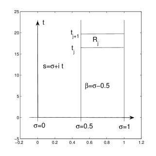
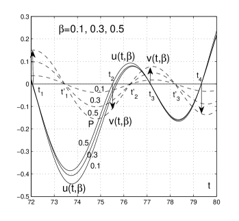
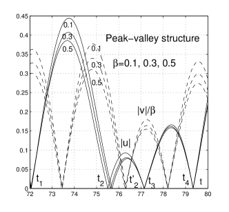
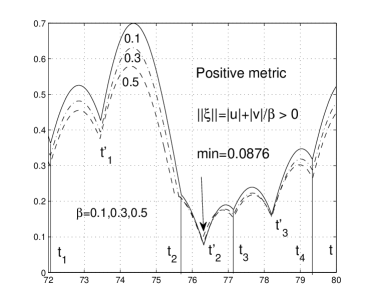
Figure 1: Fig. 1.1-4. Take $\beta=0.1,0.3,0.5$, curves $\{u,v\}$,$\{|u|,|v|/\beta\}$ and $|u|+|v|/\beta>0$.

3 Local geometric proof of RH

We shall regard $\{u(t,\beta),v(t,\beta)\}$ as a continuous changing process from $\beta=+0$ to $\beta=0.5$. For any fixed $\beta\in(0,0.5]$ the real part $u(t,\beta)$ is an irregular high-frequency oscillation, and its zeros $t_{j}$ (also depend on $\beta$) form an irregular infinite sequence

$$\begin{array}[]{lll}...<t_{j-1}<t_{j}<t_{j+1}<t_{j+2}<.....\end{array}$$

We shall take them as the base in studying peak-valley structure. We prove

Theorem 1(local peak-valley structure). For any fixed $\beta\in(0,1/2]$ and in each root-interval $I_{j}=[t_{j},t_{j+1}]$, then the curves $\{|u|,|v|/\beta\}$ form a local peak-valley structure, and $||\xi||$ has the positive low bound independent of $t\in I_{j}$,

$$\min_{t\in I_{j}}(|u|+|v|/\beta)=\mu(t_{j},\beta)>0,\ \ \ \beta\in[+0,0.5].$$ (3.1)

Proof. 1. Single peak case.

From Fig.1.2 we have seen the following general property.

Geometric property of single peak. For any $\beta\geq 0$, there are $u_{t}>0$ from negative peak to positive one, and $u_{t}<0$ from positive peak to negative one.

Below it is enough to discuss $u>0$ inside the root-interval $I_{j}$. For any fixed $\beta>0$, using Lemma 1, we discuss two cases as follows.

1). As $u_{t}>0$ near the left node $t_{j}$,we have

$$\left\{\begin{array}[]{ll}v(t_{j},\beta)/\beta&=-\displaystyle\frac{1}{\beta}\int_{0}^{\beta}u_{t}(t_{j},r)dr<0,\\ \lim\limits_{\beta\rightarrow+0}v(t_{j},\beta)/\beta&=-u_{t}(t_{j},0)<0.\end{array}\right.$$ (3.2)

2). As $u_{t}<0$ near the right node $t_{j+1}$, similarly

$$\left\{\begin{array}[]{ll}v(t_{j+1},\beta)/\beta&=\displaystyle-\frac{1}{\beta}\int_{0}^{\beta}u_{t}(t_{j+1},r)dr>0,\\ \lim\limits_{\beta\rightarrow+0}v(t_{j+1},\beta)/\beta&=-u_{t}(t_{j+1},0)>0.\\ \end{array}\right.$$ (3.3)

which are valid and numerically stable for $\beta\in[+0,1/2]$.

Because $v(t,\beta)$ has opposite signs at two end-points in $I_{j}$, there certainly exists an inner point $t^{\prime}_{j}=t^{\prime}_{j}(\beta)$ such that $v(t^{\prime}_{j},\beta)=0$. Clearly in $I_{j}$, $|u|$ is a peak curve and $|v(t,\beta)|/\beta$ is a valley curve, thus $\{|u|,|v|/\beta\}$ form a local peak-valley structure. We define a continuous function with respect to $(t,\beta)$

$$\begin{array}[]{lll}\phi(t,\beta)=|u(t,\beta)|+|v(t,\beta)|/\beta,\ \ \ \beta\in[+0,0.5],\ t\in I_{j}=[t_{j},t_{j+1}],\end{array}$$

which certainly has a positive low bound independent of $t\in I_{j}$,

$$\min_{t\in I_{j}}\phi(t,\beta)=\mu(t_{j},\beta)>0,\ \ \beta\in[+0,0.5].$$ (3.4)

This is a fine local geometric analysis.

2. Multiple peak case. Although $||\xi||>0$ is still valid, we shall prove that multiple peak case does not appear.

Assume that $u(t,\beta)>0$ inside $I_{j}=[t_{j},t_{j+1}]$, and there has odd number of positive extreme values $u(t_{jp},\beta)=a_{jp}>0$ at the inner points $t_{jp}$, $p=1,2,...,2k+1$. We consider the minimum value $u(t_{ji},\beta)$ at some point $t^{\prime}=t_{ji}$, where $u>0,u_{t}=0$ and $u_{tt}>0$, i.e., $u$ is convex toward $t$-axis. By Cauchy-Riemann condition $v_{t}=u_{\beta}$ and analytic property $u_{\beta}(t,0)=0$, we get

$$v_{t}(t^{\prime},\beta)=v_{t}(t^{\prime},0)+\int_{0}^{\beta}v_{t\beta}(t^{\prime},r)dr=-\int_{0}^{\beta}u_{tt}(t^{\prime},r)dr<0.$$ (3.5)

On the other hand, because $u>0$ inside $I_{j}$, then RH is locally valid. Using the equivalence of Lagarias [7](1999), we have

$$Re(\frac{\xi^{\prime}}{\xi})=Re(\frac{\xi^{\prime}\bar{\xi}}{|\xi|^{2}})=(uu_{\beta}+vv_{\beta})/|\xi|^{2}>0,\ \ \beta>0.$$ (3.6)

Using Cauchy-Riemann conditions $u_{\beta}=v_{t},u_{t}=-v_{\beta}$, it derives

$$\psi(t)=uv_{t}-vu_{t}>0,\ \ \beta>0.$$ (3.7)

But now, $u>0,u_{t}=0,v_{t}<0$ at $t=t^{\prime}$, which lead to contradiction $\psi=uv_{t}<0$.

Should point out that in multiple peak case for fixed $\beta>0$, the real part $u\geq a_{jl}>0$ in the subinterval $I^{*}=[t_{j1},t_{j,2k+1}]$, while in remaining subintervals $[t_{j},t_{j1}]$ and $[t_{j,2k+1},t_{j+1}]$, we can still get the positive estimates (3.2) and (3.3), therefore $||\xi||>0$ in the root-interval $I_{j}$. But the multiple peak case will imply the following danger: When $\beta>0$ is further increased, the minimum extreme value $u=a_{ji}>0$ possibly gradually is close to $t$-axis toward its convex direction, as seen in the case 3, we can not deny the possibility to contact with $t$-axis, which will lead more difficulty. Fortunately, we have proved that the multiple peak case does not appear by using the equivalence theorem of Lagarias, and extricated oneself from the difficult position.

3. The case of two zeros to be very close to each other on the critical line. We shall prove that the root-interval will be enlarged for $\beta>0$ rather than decreased, and the peak-valley structure is valid. This conclusion is also valid in the case of double root, although no double root is found in computation up to now.

Assume that $u(t,0)$ on the critical line has a solitary small interval $I^{0}=[t^{0}_{j},t^{0}_{j+1}]$, $u(t^{0}_{j},0)=0$ and $u(t^{0}_{j+1},0)=0$. There is an extreme point $t^{\prime}\in I^{0}_{j}$ such that $u(t^{\prime},0)=\epsilon>0$ and $u_{t}=0$. We consider a larger interval $I\supset I^{0}_{j}$, in which $u_{tt}<0$ and $u(t,0)$ is convex upwards, then $u_{t}>0$ for $t<t^{\prime}$ and $u_{t}<0$ for $t<t^{\prime}$. We say $\epsilon>0$ very small if $\epsilon/|u_{tt}|<<1$. An artificial example is shown in Fig.2.

Now consider small $\beta>0$, in the larger interval $I$, we have

$$\begin{array}[]{lll}u(t,\beta)&=\displaystyle u(t,0)+u_{\beta}(t,0)\beta-\int_{0}^{\beta}u_{\beta\beta}(t,r)(r-\beta)dr&as\ u_{\beta}(t,0)=0\\ &=\displaystyle u(t,0)+d,\ d=-\int_{0}^{\beta}u_{tt}(t,r)(\beta-r)dr>0&as\ u_{\beta\beta}=-u_{tt}\\ v(t,\beta)&=\displaystyle-\int_{0}^{\beta}u_{t}(t,r)dr,\ \ \ \ see\ (2.3)&as\ v_{\beta\beta}(t,0)=0\\ &=\displaystyle-u_{t}(t,0)\beta+\frac{1}{2}\int_{0}^{\beta}u_{ttt}(t,r)(r-\beta)^{2}dr,&as\ v_{\beta\beta\beta}=u_{ttt},\end{array}$$ (3.8)

which can be summarized in the following form ($\epsilon=0$ is admissible)

$$\left\{\begin{array}[]{lll}t=t^{\prime}&u(t^{\prime},\beta)=\epsilon+d>0,&v(t^{\prime},\beta)=O(\beta^{3}),\ \ as\ u_{t}(t^{\prime},0)=0,\\ t<t^{\prime}&u(t,\beta)=u(t,0)+d,&v(t,\beta)=\displaystyle-\int_{0}^{\beta}u_{t}(t,r)dr<0,\\ t>t^{\prime}&u(t,\beta)=u(t,0)+d,&v(t,\beta)=\displaystyle-\int_{0}^{\beta}u_{t}(t,r)dr>0,\\ \end{array}\right.$$ (3.9)

From this we see that $u(t,\beta)$ has removed $u(t,0)$ in parallel by a distance $d>0$ toward the direction of its convexity. Due to $u(t,0)<0$ outside $I^{0}$, there are certainly a left node $t_{j}=t_{j}(\beta)$ and a right node $t_{j+1}=t_{j+1}(\beta)$ such that $u(t,\beta)=0$. Inside the enlarged interval $I_{j}=[t_{j},t_{j+1}]$, it forms a positive peak curve for $u(t,\beta)>0$. Besides, $v(t,\beta)$ has opposite signs at two endpoints of $I_{j}$, and there certainly exists some inner point $t^{\prime\prime}$ such that $v(t^{\prime\prime},\beta)=0$, i.e., $|v|/\beta$ is a valley curve. Therefore it forms a peak-valley structure for $\{|u|,|v|/\beta\}$ in $I_{j}$.

It should be pointed out that if $u_{tt}<0$ and decreasing $u(t^{\prime},0)<0$, which belongs to the multiple peak case. This case does not appear as mentioned above.

Finally by summarizing three cases, Theorem 1 is proved.

Fig.2. Initial value $u(t^{\prime},0)=\cos(t)-1+\epsilon$, peak-valley structure for $\beta=0.2$

We have constructed an example $u(t,0)=\cos(t)-1+\epsilon,\epsilon=0.01,\beta=0.2$ in Fig.2, which has a local peak-valley structure in $I_{j}=[t_{j},t_{j+1}]$, and it is also valid for $\epsilon=0$ which is double root. Besides, we have seen in Fig.1.2 that when increasing $\beta$, the corresponding smaller interval $(t_{2},t_{3})$ is enlarged, while another neighbor larger interval $(t_{1},t_{2})$ will be decreased.

Theorem 2. RH is valid for any $(\beta,t)\in(0,0.5]\times[0,\infty)$.

Proof. Actually, for any fixed $\beta\in(0,0.5]$, an infinite sequence can be formed for the zeros $\{t_{j}(\beta)\}$ of $u(t,\beta)$, while any $t\in[0,\infty)$ must lie in some $I_{j}$ such that $||\xi||\geq\mu(t_{j},\beta)>0$. The theorem is proved.

Recall that the equivalence $Re(\frac{\xi^{\prime}}{\xi})>0$ of Lagarias in [7](1999), which is a unique equivalent theorem with $\xi^{\prime}$ up to now. We will prove the following.

Theorem 3. The peak-valley structure and RH are equivalent.

Proof. Assume that RH is valid and $u>0$ inside root-interval $I_{j}=[t_{j},t_{j+1}]$(similarly for $u<0$). By (3.7), $\psi=uv_{t}-vu_{t}>0$, for $\beta>0$. We have the following facts.

At the left node $t_{j}$, $u=0,u_{t}>0$(geometric property) and $\psi=-vu_{t}>0$, then $v<0$;

At the right node $t_{j+1}$, $u=0,u_{t}<0$ and $\psi=-vu_{t}>0$, then $v>0$.

Therefore $v$ has opposite signs at two end-points, there certainly exists an inner point $t^{\prime}_{j}\in I_{j}$ such that $v=0$, which implies local peak-valley structure. Theorem 3 is proved.

From the view-point of complex analysis, RH requires $|\xi|>0$, while from the view-point of geometry, the peak-valley structure requires stronger norm $||\xi||>0$. Both of them are equivalent. However, the local geometry property is of extreme importance, because proving the peak-valley structure is concise and intuitive.

Remark 1. In the proof of Theorem 1 we have seen that Riemann integral $\xi=K(f)$ has $\beta$-symmetry, which is independent of the speciality of $f$. Therefore we guess that for the very wide class of the fast decay function $f$, RH is still valid for $K(f)$. We have two examples. For $t\leq 110$, there are larger low bounds $(|u_{\beta}|/\beta+|v_{\beta}|)/M\geq 0.20$ and $||\xi^{\prime\prime}||/M\geq 0.28$.

Haglund[6] has discussed $\xi$ and other functions with numerical experiments, and proposed a conjecture: If function $F_{N}$ has monotonic zeros, then which implies RH. Sarnak[10] has analyzed the Grand RH of L-function, which is more difficult.

References

References

[1] E. Bombieri. Problems of the Millennium: The
Riemann Hypothesis. AMS. 107-124(2000)
[2]http://www.claymath.org.
[3] P. Borwein, S. Choi, B. Rooney, A.
Weirathmuller. The Riemann Hypothesis. Springer (2006)
[4] J. Conrey. The Riemann Hypothesis.
Notices of The AMS. 341-353(2003)
[5] H. Edwards. Riemann’s Zeta function. Mineola:
Dover Publication,Inc.(2001)
[6] J. Huglund. Some conjectures on the zeros of
approximates to the Riemann zeta-function and incomplete gamma
functions. Cent. Eur. J. Math., 9:2,302-318(2011)
[7] J. Lagarias. On a positivity property of the Riemann
-function. Acta Arith. 89:3, 213-234(1999)
[8] J. Lune, H. Riele. On the zeros of the Riemann
Zeta function in the critical strip. Part 3. Math. Comp., 41, 759-767(1983)
[9] J. Lune, H. Riele, D.Winter. On the zeros of the Riemann
Zeta function in the critical strip. Part 4. Math. Comp., 46, 667-681(1986)
[10] P. Sarnak. Problems of the Millennium: The
Riemann Hypothesis (2004).
http://www.claymath.org.
[11] S. Smale. Mathematical problems for next century.
Math. Intelligencer. 20:2, 7-15(1998)