How Many Freemasons Are There?
The Consensus Voting Mechanism in Metric Spaces

Abstract.

We study the evolution of a social group when admission to the group is determined via consensus or unanimity voting. In each time period, two candidates apply for membership and a candidate is selected if and only if all the current group members agree. We apply the spatial theory of voting where group members and candidates are located in a metric space and each member votes for its closest (most similar) candidate. Our interest focuses on the expected cardinality of the group after $T$ time periods. To evaluate this we study the geometry inherent in dynamic consensus voting over a metric space. This allows us to develop a set of techniques for lower bounding and upper bounding the expected cardinality of a group. We specialize these methods for two-dimensional metric spaces. For the unit ball the expected cardinality of the group after $T$ time periods is $\Theta(T^{\frac{1}{8}})$. In sharp contrast, for the unit square the expected cardinality is at least $\Omega(\ln T)$ but at most $O(\ln T\cdot\ln\ln T)$.

1. Introduction

This paper studies the evolution of social groups over time. In an exclusive social group, the existing group members vote to determine whether or not to admit a new member. Familiar examples include the freemasons, fraternities, membership-run sports and social clubs, acceptance to a condominium, as well as academia. To analyze the inherent dynamics we use the model of Alon, Feldman, Mansour, Oren and Tennenholtz (dyn, ). In each time period, two candidates apply for membership and the current members vote to decide if either or none of them is acceptable. The spatial model of voting is used: each person is located uniformly at random in a metric space and each group member votes for the candidate closest to them.

Alon et al. (dyn, ) analyze social group dynamics in a one-dimensional metric space, specifically, the unit interval $[0,1]$. They examine how outcomes vary under different winner determination rules, in particular, majority voting and consensus voting. In consensus voting or unanimity voting a candidate is elected if and only if the group members agree unanimously. Equivalently, every member may veto a potential candidate.

Our interest lies in the evolution of the group size under consensus voting; that is, what is the expected cardinality of the social group $G^{T}$ after $T$ time periods? In the one-dimensional setting the answer is quite simple. There, Alon et al. (dyn, ) show that under consensus voting if a candidate is elected in round $t$ then, with high probability, it is within a distance $\Theta(1/\sqrt{t})$ of one endpoint of the interval. Because the winning candidate must be closer to all group members than the losing candidate, both candidates must therefore be near the endpoints. This occurs with probability $\Theta(1/t)$. As a consequence, in a one-dimensional metric space, the expected size of the social group after $T$ time periods is $\mathbb{E}[|G^{T}|]\cong\ln T$. Here we use the notation $f\cong g$ if both $f\lesssim g$ and $g\lesssim f$, where $f\lesssim g$ if $f\leq c\cdot g$ for some constant $c$.

Bounding the expected group size in higher-dimensional metric spaces is more complex and is the focus of this paper. To do this, we begin in Section 2 by examining the geometric aspects of consensus voting in higher-dimensional metric spaces. More concretely, we explain how winner determination relates to the convex hull of the group members and the Voronoi cells formed by the candidates. This geometric understanding enables us to construct, in Section 3, a set of techniques, based upon cap methods in probability theory, that allow for the upper bounding and lower bounding of expected group size. In Sections 4 and 5, we specialize these techniques to two-dimensions for application on the fundamental special cases of the unit square and the unit ball. Specifically, for the unit square we show the following lower and upper bounds on expected group size.

Theorem 1.1.

Let the metric space be the unit square $\mathbb{H}$. Then the expected cardinality of the social group after $T$ periods is bounded by  $\ln T\ \lesssim\ \mathbb{E}[\,|G^{T}|\,]\ \lesssim\ \ln T\cdot\ln\ln T$.

Thus, expected group size for the two-dimensional unit square is comparable to that of the one-dimensional interval. Surprisingly, there is a dramatic difference in expected group size between the unit square and the unit ball. For the unit ball, the expected group size evolves not logarithmically but polynomially with time.

Theorem 1.2.

Let the metric space be the unit ball $\mathbb{B}$. Then the expected cardinality of the social group after $T$ periods is  $\mathbb{E}[\,|G^{T}|\,]\ \cong\ T^{\frac{1}{8}}$.

1.1. Background and Related Work

Here we discuss some background on the spatial model and consensus voting. The spatial model of voting utilized in this paper dates back nearly a century to the celebrated work of Hotelling (harold1929stability, ). His objective was to study the division of a market in a duopoly when consumers are distributed over a one-dimension space, but he noted his work had intriguing implications for electoral systems. Specifically, in a two-party system there is an incentive for the political platforms of the two parties to converge. This was formalized in the median voter theorem of Black (Bla48, ): in a one-dimensional ideological space the location of the median voter induces a Condorcet winner, given single-peaked voting preferences. The traditional voting assumption in a metric space is proximity voting where each voter supports its closest candidate; observe that proximity voting gives single-peaked preferences.

The spatial model of voting was formally developed by Downs (Dow57, ) in 1957, again in a one-dimensional metric space. Davis, Hinich, and Ordeshook (DHO70, ) expounded on practical necessity of moving beyond just one dimension. Interestingly, they observed that in two-dimensional metric spaces, a Condorcet winner is not guaranteed even with proximity voting. Of particular relevance here is their finding that, in dynamic elections, the order in which candidates are considered can fundamentally affect the final outcome (Bla48, ; DHO70, ).

There is now a vast literation on spatial voting, especially concerning the strategic aspects of simple majority voting; see, for example, the books (enelow1984spatial, ; arrow1990advances, ; merrill1999unified, ; Poo05, ; Sch07, ). There has also been a vigorous debate concerning whether voter utility functions in spatial models should be distance-based (such as the standard assumption of proximity voting used here), relational (e.g. directional voting (RS89, )), or combinations thereof (merrill1999unified, ). This debate has been philosophical, theoretical and experimental (Gro73, ; Mat79, ; LK00, ; TV08, ; Cla09, ; LP10, ). Recently there has also been a large amount of interest in the spatial model by the artificial intelligence community (ABJ15, ; FFG16, ; AJ17, ; SE17, ; BLS19, ). It is interesting to juxtapose these modern potential applications with the original motivations suggested by Black (Bla48, ), such as the administration of colonies!

Consensus is one of the oldest group decision-making procedures. In addition to exclusive social groups, it is familiar in a range of disparate settings, including judicial verdicts, Japanese corporate governance (vogel1975modern, ), and even decision making in religious groups, such as the Quakers (hare1973group, ). From a theoretic perspective, consensus voting in a metric spaces has also been studied by Colomer (colomer1999geometry, ) who highlights the importance the initial set of voters can have on outcomes in a dynamic setting.

2. The Geometry of Consensus Voting

In this section, we present a simple geometric interpretation of a single election using consensus voting in the spatial model. In the subsequent sections, we will apply this understanding, developed for the static case, to study the dynamic model. Specifically, we examine how a group grows over time when admission to the group is via a sequence of consensus elections.

Let $G^{0}=\{v_{1},\cdots,v_{k}\}$ denote the initial set of group members, selected uniformly and independently from a metric space $K$. In the consensus voting mechanism, for each round $t\geq 1$, a finite set of candidates $C^{t}=\{w_{1},\cdots,w_{n}\}\subseteq K$ applies for membership. Members of the group at the start of round $t$, denoted $G^{t-1}$, are eligible to vote. Assuming the spatial theory of voting, each group member will vote for the candidate who is closest to her in the metric space. That is, member $v_{i}$ votes for candidate $w_{j}$ if and only if $d(v_{i},w_{j})\leq d(v_{i},w_{k})$ for every candidate $w_{k}\neq w_{j}$. Under the consensus (unanimity) voting rule, if every group member selects the candidate $w_{j}\in C^{t}$ then $w_{j}$ is accepted to the group and $G^{t}=G^{t-1}\cup w_{j}$; otherwise, if the group does not vote unanimously then no candidate wins selection and $G^{t}=G^{t-1}$.

As stated, to study how group size evolves over time, our first task is to develop a more precise understanding of when a candidate will be selected under consensus voting in a single election. Fortunately, there is a nice geometric characterization for this property in terms of the Voronoi cells (regions) formed in the metric space $K$ by the candidates (points) $C=\{w_{1},\cdots w_{n}\}$. Specifically, the Voronoi cell $H_{i}$ associated with point $w_{i}$ is $H_{i}:=\{v\in K\ |\ d(v,w_{i})\leq d(v,w_{j})\ \text{for all }i\neq j\}$. We will see that the convex hull of the group members $G\subseteq K$, which we denote $S=conv(G)$, plays an important role in winner determination. The characterization theorem for the property that a candidate is selected under the consensus voting mechanism is then:

Theorem 2.1.

Let $C=\{w_{1},w_{2},\dots,w_{n}\}$ be the candidates and let $H_{1},H_{2},\dots,H_{n}$ be the Voronoi cells on $K$ generated by $C$. Then there is a winner under consensus voting if and only if $S=conv(G)\subseteq H_{i}$ for some candidate $w_{i}$.

Proof.

Assume $S=\subseteq H_{i}$ for some candidate $w_{i}\in C$. Then, for every voter $v_{j}\in G$, we have $d(v_{j},w_{i})\leq d(v_{j},w_{k})$ for any other candidate $w_{k}\in C$. Hence, every voter prefers candidate $w_{i}$ over all the other candidates. Thus candidate $w_{i}$ is selected. Conversely, assume that candidate $w_{i}$ is selected. Then, by definition of consensus voting, each voter $v_{j}\in G$ voted for $w_{i}$. Thus $d(v_{j},w_{i})\leq d(v_{j},w_{k})$ for all $k\neq i$. Ergo, $G\subseteq S\subseteq H_{i}$. ∎

Several useful facts can be derived from this characterization. These facts are stated in the subsequent corollary and lemma.

Corollary 2.2.

Let $C=\{w_{1},w_{2},\dots,w_{n}\}$ be set of candidates. If there is a candidate accepted with $S=A$, then the same candidate is also accepted with $S=B$ for any convex set $B\subseteq A$.

Proof.

By Theorem 2.1, a candidate is accepted if and only if the current convex hull is entirely contained within one of Voronoi regions, $H_{1},H_{2},\dots,H_{n}$, generated by the candidates. Clearly, if $A\subseteq H_{i}$ then $B\subseteq H_{i}$. Therefore, if there is an acceptance with $S=A$ then there would be an acceptance with $S=B$. The result follows immediately. ∎

The next lemma requires the following definition: let $B(v,w)$ denote the Euclidean ball centred at $v$ with radius $\|w-v\|$. Furthermore, we denote by $\partial S$ the set of vertices (extreme points) of the convex hull $S$ of the group members. Observe that $\text{conv}(\partial S)=S$ and that $\partial S\subseteq G$.

Lemma 2.3.

Let $G$ be current set of group members and $S$ be its convex hull. Let $C=\{w_{1},w_{2},\cdots,w_{n}\}$ be the current candidates. Under consensus, there is a winning candidate if and only if $\exists w_{i}\in C$ such that

$$w_{i}\in\bigcap\limits_{k\in[n]\setminus i}\,\bigcap\limits_{v_{j}\in\partial S}B(v_{j},w_{k})$$

Proof of Lemma 2.3.

If there is a consensus then there is a $w_{i}\in C$ who is selected. Hence among all candidates, $w_{i}$ is closest to each group member. That is, $d(v_{j},w_{i})\leq d(v_{j},w_{k})$, for each group member $v_{j}\in G$ and each candidate $w_{k}\in C\setminus w_{i}$. It follows that

$$w_{i}\in\bigcap\limits_{k\in[n]\setminus i}\,\bigcap\limits_{v_{j}\in G}B(v_{j},w_{k})\subseteq\bigcap\limits_{k\in[n]\setminus i}\,\bigcap\limits_{v_{j}\in\partial S}B(v_{j},w_{k})$$

where the last inclusion holds since $\partial S\subseteq G$. Conversely, suppose there exists a $w_{i}$ such that $w_{i}\in\bigcap\limits_{k\in[n]\setminus i}\bigcap\limits_{v_{j}\in\partial S}B(v_{j},w_{k})$. Thus, $w_{i}$ satisfies $d(v_{j},w_{i})\leq d(v_{j},w_{k})$ for each voter $v_{j}\in\partial S$ and $w_{k}\in C\setminus w_{i}$. Hence we have $\partial S\subseteq H_{i}$, which implies $\text{conv}(\partial S)=S\subseteq\text{conv}(H_{i})=H_{i}$ as $H_{i}$ is convex. Therefore $G\subseteq S\subseteq H_{i}$. Thus, by Theorem 2.1, candidate $w_{i}$ wins under consensus voting. ∎

Following Alon et al. (dyn, ), from now on we restrict attention to case of $n=2$ candidates in each round. The case $n\geq 3$ is not conceptually harder and the ideas presented in this paper do extend to that setting, but mathematically the analyses would be even more involved than those that follow.

3. General Tools for Bounding Expected Group Size

In this section we introduce a general approach for obtaining both upper and lower bounds on the expected cardinality of the social group in round $t$. These techniques apply for consensus voting in any convex compact domain $K$. In the rest of the paper we will specialize these methods for the cases in which $K$ is either a unit ball or a unit square. In particular, lower bounds are provided for these two domains in Section 4 and upper bounds in Section 5.

Let $K$ be a convex compact set, and let $C^{t}=\{w_{1},w_{2}\}$ be candidates appearing in round $t$. We assume each candidate $w_{i}$ is distributed uniformly on $K$. We may also assume that $\text{vol}(K)=1$, as otherwise we can absorb the associated constant factor into our bounds. Note that the expected group size is $\mathbb{E}[|G^{T}|]=\sum_{t=1}^{T}\Pr[X^{t}]$, where $X^{t}$ denotes the event a new candidate wins in round $t$.

Let’s first present the intuition behind our approach to upper bounding the probability of selecting a candidate in any round. Recall that, by Theorem 2.1, given two candidates $\{w_{1},w_{2}\}$ in round $t+1$, we accept candidate $i$ if and only if $S^{t}\subseteq H_{i}(w_{1},w_{2})$. Now in order for the convex hull to satisfy $S^{t}\subseteq H_{i}(w_{1},w_{2})$, it must be the case that in the previous round (i) $S^{t-1}\subseteq H_{i}(w_{1},w_{2})$, and (ii) a new candidate did not get accepted inside the complement $\mkern 1.5mu\overline{\mkern-1.5muH_{i}(w_{1},w_{2})\mkern-1.5mu}\mkern 1.5mu={\bf cl}(K\setminus H_{i}(w_{1},w_{2}))$, where ${\bf cl}$ denotes set closure. Applying this argument recursively with respect to the worst case convex hulls for accepting candidates inside $\mkern 1.5mu\overline{\mkern-1.5muH_{i}(w_{1},w_{2})\mkern-1.5mu}\mkern 1.5mu$, we will obtain an upper bound on the probability of accepting a candidate. Such worst case convex hulls can be found by appropriately applying Corollary 2.2.

To formalize this intuition, we require some more notation. We denote by $Z(H)$ the event that a new candidate is selected inside $H$. Let $\Pr[Z(H)|S=A]$ denote the probability of selecting a candidate inside $H$ given the convex hull of the group members is $A$. The shorthand $\Pr[Z(H)|A]=\Pr[Z(H)|S=A]$ will be used when the context is clear. Note, by Lemma 2.3, the probability of acceptance depends only on the shape of the convex hull of the members, and not on the round. That is, if $S^{t}=S^{\hat{t}}=A$ for two rounds $t\neq\hat{t}$ then the probabilities of accepting a candidate inside a given region in the rounds $t+1$ and $\hat{t}+1$ are exactly the same.

We say a set $A$ is a cap if there exists a half space $W$ such that $A=K\cap W$. We remark that caps have been widely used for studying the convex hull of random points; see the survey article (baddeley2007random, ) and the references therein. Of particular relevance here is that, in the case of two candidates, the Voronoi regions for the candidates are caps. Furthermore, $\mkern 1.5mu\overline{\mkern-1.5muH_{1}(w_{1},w_{2})\mkern-1.5mu}\mkern 1.5mu=H_{2}(w_{1},w_{2})$ and vice versa.

Theorem 3.1.

Let $K$ be convex compact domain and let $f_{K}(w_{1},w_{2})$ be any function which satisfies $f_{K}(w_{1},w_{2})\leq\min\limits_{i}\Pr[Z(H_{i}(w_{1},w_{2}))\ |\ \mkern 1.5mu\overline{\mkern-1.5muH_{i}(w_{1},w_{2})\mkern-1.5mu}\mkern 1.5mu]$. Then

$$\Pr[X^{t+1}]\ \lesssim\ \int_{K}\int_{K}e^{-tf_{K}(w_{1},w_{2})}\,dw_{1}\,dw_{2}$$

Proof.

Observe that, for any cap $A$, we have the following inequality:

$$\Pr[S^{t}\subseteq A]\ =\ \left(1-\Pr[Z(\mkern 1.5mu\overline{\mkern-1.5muA\mkern-1.5mu}\mkern 1.5mu)\ |\ S^{t-1}\subseteq A]\right)\cdot\Pr[S^{t-1}\subseteq A]$$

$$\ \leq\ \left(1-\Pr[Z(\mkern 1.5mu\overline{\mkern-1.5muA\mkern-1.5mu}\mkern 1.5mu)\ |\ S^{t-1}=A]\right)\cdot\Pr[S^{t-1}\subseteq A]$$

(1) $$\ \leq\ \left(1-\Pr[Z(\mkern 1.5mu\overline{\mkern-1.5muA\mkern-1.5mu}\mkern 1.5mu)\ |\ A\ ]\right)^{t}$$

Here the first inequality follows from Corollary 2.2. The second inequality is obtained by repeating the argument inductively for $S^{t-1}$. Hence:

$$\Pr[X^{t+1}] \ =\ \int\int\Pr[X^{t+1}\ |\ (w_{1},w_{2})\ \text{are candidates}]\,dw_{1}\,dw_{2}$$

$$\ =\ \int\int\big{(}\Pr[S^{t}\subseteq H_{1}(w_{1},w_{2})]+\Pr[S^{t}\subseteq H_{2}(w_{1},w_{2})]\big{)}\,dw_{1}\,dw_{2}$$

$$\ \leq\ \sum_{i=1}^{2}\,\int\int\big{(}1-\Pr[Z(H_{i}(w_{1},w_{2}))\ |\ \mkern 1.5mu\overline{\mkern-1.5muH_{i}(w_{1},w_{2})\mkern-1.5mu}\mkern 1.5mu\ ]\big{)}^{t}\,dw_{1}\,dw_{2}$$

$$\ \leq\ 2\int\int(1-f_{K}(w_{1},w_{2}))^{t}\,dw_{1}\,dw_{2}$$

$$\ \leq\ 2\int\int e^{-tf_{K}(w_{1},w_{2})}\,dw_{1}\,dw_{2}$$

The second equality holds by Theorem 2.1. The first inequality follows by combining inequality (1) and the facts $\mkern 1.5mu\overline{\mkern-1.5muH_{1}(w_{1},w_{2})\mkern-1.5mu}\mkern 1.5mu=H_{2}(w_{1},w_{2})$ and $\mkern 1.5mu\overline{\mkern-1.5muH_{2}(w_{1},w_{2})\mkern-1.5mu}\mkern 1.5mu=H_{1}(w_{1},w_{2})$. Next, by assumption, $f_{K}(w_{1},w_{2})\leq\Pr[Z(H_{i}(w_{1},w_{2}))\ |\ \mkern 1.5mu\overline{\mkern-1.5muH_{i}(w_{1},w_{2})\mkern-1.5mu}\mkern 1.5mu]$ for each $i$; the last two inequalities follow immediately. ∎

As stated, Theorem 3.1 allows us to upper bound the expected group size. However, the theorem is not easily applicable on its own. To rectify this, consider the following easier to apply corollary.

Corollary 3.2.

Let $K$ be compact space. If $f_{K}$ satisfies the conditions of Theorem 3.1 then

$$\Pr[X^{t+1}]\ \lesssim\ \frac{1}{t}+\int_{0}^{\frac{\ln(t)}{t}}te^{-t\lambda}\cdot\Phi(\lambda)\,d\lambda$$

where $\Phi(\lambda)=\int\int\mathbb{I}\left[f_{K}(w_{1},w_{2})\leq\lambda\right]dw_{1}dw_{2}$.

Proof of Corollary 3.2.

From Theorem 3.1, we have that,

$$\Pr[X^{t+1}] \ \lesssim\ \int\int\mathbb{I}\left[f_{K}(w_{1},w_{2})\leq\frac{\ln(t)}{t}\right]\cdot e^{-tf_{K}(w_{1},w_{2})}\,dw_{1}\,dw_{2}$$

$$\quad\quad\quad+\ \int\int\mathbb{I}\left[f_{K}(w_{1},w_{2})\geq\frac{\ln(t)}{t}\right]\cdot e^{-tf_{K}(w_{1},w_{2})}\,dw_{1}\,dw_{2}$$

(2) $$\ \leq\ \int\int\mathbb{I}\left[f_{K}(w_{1},w_{2})\leq\frac{\ln(t)}{t}\right]\cdot e^{-tf_{K}(w_{1},w_{2})}\,dw_{1}\,dw_{2}\ +\ \frac{1}{t}\leavevmode\nobreak\$$

Next, consider the random variable $Y=f_{K}(w_{1},w_{2})$ and denote its cumulative distribution function by $F_{Y}(\lambda)=\Pr[Y\leq\lambda]=\Phi(\lambda)$. Then

$$\int\int\mathbb{I}\left[f_{K}(w_{1},w_{2})\leq\frac{\ln(t)}{t}\right]\cdot e^{-tf_{K}(w_{1},w_{2})}\,dw_{1}\,dw_{2} \ =\ \mathbb{E}\left[\mathbb{I}\left[f_{K}(w_{1},w_{2})\leq\frac{\ln(t)}{t}\right]\cdot e^{-tf_{K}(w_{1},w_{2})}\right]$$

$$\ =\ \mathbb{E}_{Y}\left[\mathbb{E}\left[\mathbb{I}\left[Y\leq\frac{\ln(t)}{t}\right]\cdot e^{-tY}\ |\ Y\right]\right]$$

(3) $$\ =\ \int_{0}^{1}\mathbb{I}\left[\lambda\leq\frac{\ln(t)}{t}\right]\cdot e^{-t\lambda}\ dF_{Y}(\lambda)$$

The second equality is due to the law of total expectation. Now, because $F_{Y}$ is absolutely continuous it has a density function. Combining (2) and (3), we then have that

$$\Pr[X^{t+1}]\ \lesssim\ \frac{1}{t}+\int_{0}^{\frac{\ln(t)}{t}}e^{-t\lambda}\cdot\frac{d}{d\lambda}\,\Phi(\lambda)\,d\lambda$$

$$\ =\ \frac{1}{t}+\left[e^{-{t\lambda}}\Phi(\lambda)\right]_{0}^{\frac{\ln(t)}{t}}+\int_{0}^{\frac{\ln(t)}{t}}te^{-t\lambda}\cdot\Phi(\lambda)\,d\lambda$$

$$\ \lesssim\ \frac{1}{t}+\int_{0}^{\frac{\ln(t)}{t}}te^{-t\lambda}\cdot\Phi(\lambda)\,d\lambda$$

Here the last inequality was obtained by noting $\Phi(0)=0$ and $\Phi(\lambda)\leq 1$. ∎

As alluded to earlier, when obtaining upper bounds for the unit ball and the unit square, we will apply Corollary 3.2. Of course, in order to do this, we must find an appropriate function $f_{K}(w_{1},w_{2})$ which lower bounds the probability of acceptance inside a Voronoi region $H_{i}(w_{1},w_{2})$, given the current convex hull is $\mkern 1.5mu\overline{\mkern-1.5muH_{i}(w_{1},w_{2})\mkern-1.5mu}\mkern 1.5mu$. Finding such a function $f_{K}$ can require some ingenuity, but Lemma 3.3 below will be useful in assisting in this task. Moreover, as we will see in Section 4, this lemma can be used to obtain lower bounds as well as upper bounds on the expected cardinality of the group.

Lemma 3.3.

Given a two-dimensional convex compact domain $K$ and a cap $A$. If $z_{1}$ and $z_{2}$ are the endpoints of the line segment separating $A$ and $\mkern 1.5mu\overline{\mkern-1.5muA\mkern-1.5mu}\mkern 1.5mu$ then

$$\Pr[Z(A)\ |\ \mkern 1.5mu\overline{\mkern-1.5muA\mkern-1.5mu}\mkern 1.5mu\ ]\ =\ 2\cdot\int_{A}\text{vol}(B(z_{1},\xi)\cap B(z_{2},\xi)\cap A)\ d\xi$$

Proof.

Without loss of generality, let $w_{2}\in A$ be the selected candidate. Thus, by Theorem 2.1, we have $\mkern 1.5mu\overline{\mkern-1.5muA\mkern-1.5mu}\mkern 1.5mu\subseteq H_{2}(w_{1},w_{2})$ because, by assumption, the convex hull of the voters is $S=\mkern 1.5mu\overline{\mkern-1.5muA\mkern-1.5mu}\mkern 1.5mu$. We claim $w_{1}\notin\mkern 1.5mu\overline{\mkern-1.5muA\mkern-1.5mu}\mkern 1.5mu$. Otherwise, $w_{1}\in\mkern 1.5mu\overline{\mkern-1.5muA\mkern-1.5mu}\mkern 1.5mu\subseteq H_{2}(w_{1},w_{2})$. But, by definition of the Voronoi regions, we have $w_{1}\in H_{1}(w_{1},w_{2})$. Thus, $w_{1}\in H_{1}\cap H_{2}$. However, this cannot happen unless $w_{1}=w_{2}$, a zero probability event. Therefore, we may assume that $w_{1},w_{2}\in A$.

Next, consider the line $l(z_{1},z_{2})$ separating $A$ and $\mkern 1.5mu\overline{\mkern-1.5muA\mkern-1.5mu}\mkern 1.5mu$; that is, $l(z_{1},z_{2})$ is the convex hull $\text{conv}(z_{1},z_{2})$. Given $w_{1},w_{2}\in A$ we claim $l(z_{1},z_{2})\subseteq H_{2}(w_{1},w_{2})$ if and only if $\mkern 1.5mu\overline{\mkern-1.5muA\mkern-1.5mu}\mkern 1.5mu\subseteq H_{2}(w_{1},w_{2})$. First assume $\mkern 1.5mu\overline{\mkern-1.5muA\mkern-1.5mu}\mkern 1.5mu\subseteq H_{2}(w_{1},w_{2})$. As $\bar{A}$ is closed, $z_{1}$ and $z_{2}$ are in $\bar{A}$. Thus, by convexity, $l(z_{1},z_{2})\subseteq\bar{A}\subseteq H_{2}(w_{1},w_{2})$. On the other hand, assume $l(z_{1},z_{2})\subseteq H_{2}(w_{1},w_{2})$ and consider the Voronoi edge defined by $E(w_{1},w_{2})=H_{1}(w_{1},w_{2})\cap H_{2}(w_{1},w_{2})$. Then either $E(w_{1},w_{2})\subseteq A$ or $E(w_{1},w_{2})\subseteq\mkern 1.5mu\overline{\mkern-1.5muA\mkern-1.5mu}\mkern 1.5mu$ because $l(z_{1},z_{2})$ separates $A$ and $\mkern 1.5mu\overline{\mkern-1.5muA\mkern-1.5mu}\mkern 1.5mu$ and, by assumption, $l(z_{1},z_{2})\subseteq H_{2}(w_{1},w_{2})$. Furthermore, observe that the midpoint $\frac{1}{2}(w_{1}+w_{2})$ is in $E(w_{1},w_{2})$ and in $A$. So it must be the case that $E(w_{1},w_{2})\subseteq A$. But if $E(w_{1},w_{2})\subseteq A$ then one of the Voronoi regions contains $\mkern 1.5mu\overline{\mkern-1.5muA\mkern-1.5mu}\mkern 1.5mu$. In particular, $\mkern 1.5mu\overline{\mkern-1.5muA\mkern-1.5mu}\mkern 1.5mu\subseteq H_{2}(w_{1},w_{2})$ because $l(z_{1},z_{2})\subseteq H_{2}(w_{1},w_{2})$. Therefore,

$$\Pr[Z(A)\ |\ \mkern 1.5mu\overline{\mkern-1.5muA\mkern-1.5mu}\mkern 1.5mu\ ] \ =\ 2\int_{A}\int_{A}\mathbb{I}[\mkern 1.5mu\overline{\mkern-1.5muA\mkern-1.5mu}\mkern 1.5mu\subseteq H_{2}(w_{1},w_{2})]\ dw_{2}\,dw_{1}$$

$$\ =\ 2\ \int_{A}\int_{A}\mathbb{I}[l(z_{1},z_{2})\subseteq H_{2}(w_{1},w_{2})]\ dw_{2}\,dw_{1}$$

$$\ =\ 2\ \int_{A}\text{vol}(B(z_{1},w_{1})\cap B(z_{2},w_{1})\cap A)\,dw_{1}$$

Here the first equality holds since two candidates are equally likely to win by symmetry and, by Theorem 2.1, the winning candidate $w_{2}$ satisfies $\mkern 1.5mu\overline{\mkern-1.5muA\mkern-1.5mu}\mkern 1.5mu\subseteq H_{2}(w_{1},w_{2})$. The second equality follows from the fact that $l(z_{1},z_{2})\subseteq H_{2}(w_{1},w_{2})$ if and only if $\mkern 1.5mu\overline{\mkern-1.5muA\mkern-1.5mu}\mkern 1.5mu\subseteq H_{2}(w_{1},w_{2})$ when $w_{1},w_{2}\in A$. Finally, the last equality holds because, by Lemma 2.3, we know that any candidate $w_{2}\in B(z_{1},w_{1})\cap B(z_{2},w_{1})$ is selected with consensus voting. This is equivalent to $l(z_{1},z_{2})\subseteq H_{2}(w_{1},w_{2})$, by Theorem 2.1. ∎

4. Lower bounds on Expected Group Size

In this section we provide lower bounds for the cases where $K$ is either a unit ball $\mathbb{B}$ or a unit square $\mathbb{H}$. Recall, we assumed that $\text{vol}(K)=1$ but $\text{vol}(\mathbb{B})=\pi$ for the unit ball. We remark that this is of no consequence as we may absorb the associated constant factor into our bounds.

4.1. Lower Bound for the Unit Ball

For the unit ball $\mathbb{B}$, a circular segment is the small piece of the circle formed by cutting along a chord. Evidently, this means that every cap of $\mathbb{B}$ is either a circular segment or the complement of a circular segment. Thus, to analyze the case of the unit ball we must study circular segments.

Lemma 4.1.

Let $\mathbb{B}$ be a unit ball, and $J_{\delta}$ be a circular segment with height $\delta\leq\frac{1}{8}$ then

$$\Pr[Z(J_{\delta})\ |\ \mkern 1.5mu\overline{\mkern-1.5muJ_{\delta}\mkern-1.5mu}\mkern 1.5mu\ ]\gtrsim\delta^{4}$$

Proof.

Let $z_{1}$ and $z_{2}$ be the endpoints of the chord defining the line segment $J_{\delta}$. By rotating the ball, we may assume the chord is horizontal. Furthermore, by translating the coordinates, we may assume that $z_{1}$ lies at the origin. This is illustrated in Figure 1.

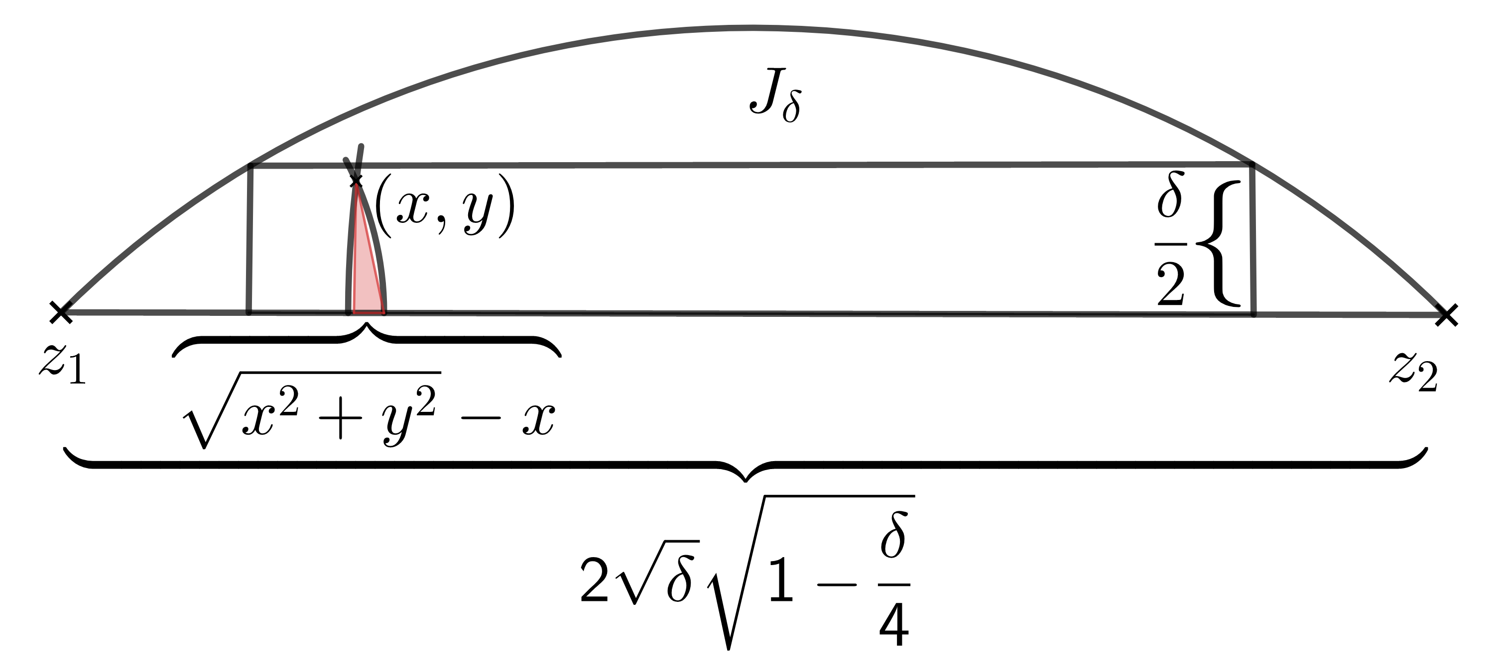
Figure 1. The circular segment $J_{\delta}$ with inscribed rectangle $R$ of height $\frac{\delta}{2}$

To apply Lemma 3.3, let $\xi=(x,y)$. Observe that the region $B(z_{1},\xi)\cap B(z_{2},\xi)\cap J_{\delta}$ contains a triangle $T$ of height $y$ and width $\sqrt{x^{2}+y^{2}}-x$. Again, this is shown in Figure 1. It follows that

(4) $$\text{vol}(B(z_{1},\xi)\cap B(z_{2},\xi)\cap J_{\delta})\ \geq\ \frac{1}{2}y\cdot(\sqrt{x^{2}+y^{2}}-x)\ \geq\ \frac{y^{3}}{4(x+y)}$$

To obtain inequality (4) first observe, by Bernoulli’s Inequality, that $\sqrt{1+\frac{y^{2}}{x^{2}}}\leq 1+\frac{1}{2}\frac{y^{2}}{x^{2}}$. This implies $\left(1+\frac{y^{2}}{x^{2}}\right)-\sqrt{1+\frac{y^{2}}{x^{2}}}\geq\frac{1}{2}\frac{y^{2}}{x^{2}}$. Rearranging terms, we obtain $(x^{2}+y^{2})-x\sqrt{x^{2}+y^{2}}\geq\frac{y^{2}}{2}$. Equivalently, $\sqrt{x^{2}+y^{2}}-x\geq\frac{y^{2}}{2\sqrt{x^{2}+y^{2}}}\geq\frac{y^{2}}{2(x+y)}$, as required. Combining Lemma 3.3 with inequality (4) then gives

(5) $$\Pr[Z(J_{\delta})\ |\ \mkern 1.5mu\overline{\mkern-1.5muJ_{\delta}\mkern-1.5mu}\mkern 1.5mu\ ]\ \geq\ \int_{J_{\delta}}\,\text{vol}(B(z_{1},\xi)\cap B(z_{2},\xi)\cap J_{\delta})\ d\xi\ \geq\ \int_{J_{\delta}}\frac{y^{3}}{4(x+y)}\ dx\,dy$$

To lower bound this integral, rather than integrate over the entire circular segment $J_{\delta}$, we will integrate over an inscribe rectangle. Specifically let $R$ be the rectangle of height $\frac{1}{2}\delta$ inscribed inside $J_{\delta}$. This rectangle, shown in Figure 1, has width $2\sqrt{1-(1-\frac{\delta}{2})^{2}}=2\sqrt{\delta}\cdot\sqrt{1-\frac{\delta}{4}}$ and is centred at $x=\sqrt{\delta}\cdot\sqrt{2-\delta}$. Therefore,

$$\int_{J_{\delta}}\,\frac{y^{3}}{4(x+y)}\ dx\,dy \ \geq\ \int_{R}\,\frac{y^{3}}{4(x+y)}\ dx\,dy$$

$$\ =\ \int_{0}^{\frac{\delta}{2}}\int^{\sqrt{\delta}(\sqrt{2-\delta}+\sqrt{1-\frac{\delta}{4}})}_{\sqrt{\delta}(\sqrt{2-\delta}-\sqrt{1-\frac{\delta}{4}})}\frac{y^{3}}{4(x+y)}\ dx\,dy$$

$$\ \geq\ \frac{1}{8}\cdot\int_{0}^{\frac{\delta}{2}}\int^{\sqrt{\delta}(\sqrt{2-\delta}+\sqrt{1-\frac{\delta}{4}})}_{\sqrt{\delta}(\sqrt{2-\delta}-\sqrt{1-\frac{\delta}{4}})}\frac{y^{3}}{x}\ dx\,dy$$

$$\ \gtrsim\ \int_{0}^{\frac{\delta}{2}}y^{3}\cdot\Big{[}\ln x\Big{]}^{\sqrt{\delta}(\sqrt{2-\delta}+\sqrt{1-\frac{\delta}{4}})}_{\sqrt{\delta}(\sqrt{2-\delta}-\sqrt{1-\frac{\delta}{4}})}\ dy$$

$$\ \gtrsim\ \delta^{4}\cdot\ln\left(\frac{\sqrt{2-\delta}+\sqrt{1-\frac{\delta}{4}}}{\sqrt{2-\delta}-\sqrt{1-\frac{\delta}{4}}}\right)$$

(6) $$\ \gtrsim\ \delta^{4}$$

The second inequality holds because $\delta\leq\frac{1}{8}$; specifically, when $\delta\leq\frac{1}{8}$ the circular segment lies under the line $y=x$. Thus, every point inside the circular segment satisfies $y\leq x$. The last inequality follows by observing that the logarithmic term is lower bounded by $\ln\left(\frac{\sqrt{2-\frac{1}{8}}+\sqrt{1-\frac{1}{32}}}{\sqrt{2}-\sqrt{1-\frac{1}{32}}}\right)\geq\ln 5$. Combining the inequalities (5) and (4.1) completes the proof. ∎

Note that Lemma 4.1 can be used to prove lower bound on the expected cardinality of the group. It is also used in later sections to obtain appropriate function $f_{K}$ when using Corollary 3.2.

Theorem 4.2.

For the unit ball $\mathbb{B}$, the expected group size after $T$ rounds is $\mathbb{E}[|G^{T}|]\gtrsim T^{\frac{1}{8}}$.

Proof.

For each $t$, we construct collection $\{A_{1}^{t},A_{2}^{t},\dots,A_{N(t)}^{t}\}$ of disjoint circular segments on the unit ball. To do this, let the height of each circular segment in the collection be $\delta(t)=\frac{1}{4t^{\frac{1}{4}}}$.Then we can fit $N(t)=\left\lfloor\pi\cdot t^{\frac{1}{8}}\right\rfloor$ of these segments into $\mathbb{B}$. To see this, observe that a circular segment of height $\delta$ has a chord of length $2\sqrt{\delta}\sqrt{2-\delta}$. The central angle of the segment is then $\theta=2\arctan\left(\frac{\sqrt{\delta}\sqrt{2-\delta}}{1-\delta}\right)\leq 4\sqrt{\delta}$, implying the existence of at least $N=\left\lfloor\frac{\pi}{2\sqrt{\delta}}\right\rfloor$ disjoint circular segments of height $\delta$. Now define $\tau\leq T$ to be the last round for which $\Pr[S^{\tau}\cap A_{i}^{\tau}\neq\emptyset]\geq\frac{1}{2}$. Thus,

(7) $$\mathbb{E}[|G^{\tau}|]\geq\sum_{i=1}^{N(\tau)}\Pr[S^{\tau}\cap A_{i}^{\tau}\neq\emptyset]=N(\tau)\cdot\Pr[S^{\tau}\cap A_{1}^{\tau}\neq\emptyset]\geq\frac{1}{2}\left\lfloor\pi\tau^{\frac{1}{8}}\right\rfloor\gtrsim{\tau}^{\frac{1}{8}}$$

Here, the first inequality follows from the observation that if $S^{t}\cap A_{i}^{t}\neq\emptyset$ then there is a least one group member inside $A_{i}^{t}$. The equality is due to symmetry; that is, $\Pr[S^{t}\cap A_{i}^{t}\neq\emptyset]=\Pr[S^{t}\cap A_{j}^{t}\neq\emptyset]$ for each pair $1\leq i,j\leq N(t)$. The second inequality follows because, by definition, $\Pr[S^{\tau}\cap A_{i}^{\tau}\neq\emptyset]\geq\frac{1}{2}$. Next consider rounds $t>\tau$. For these rounds, by definition of $\tau$, we know $\Pr[S^{t}\cap A_{i}^{t}\neq\emptyset]\leq\frac{1}{2}$ which implies $\Pr[S^{t}\cap A_{i}^{t}=\emptyset]\geq\frac{1}{2}$. Therefore,

$$\Pr[X^{t+1}] \ \gtrsim\ \sum_{i=1}^{N(t)}\Pr\left[Z(A^{t}_{i})\ \wedge\ \left(S^{t}\cap A^{t}_{i}=\emptyset\right)\right]$$

$$\ =\ N(t)\cdot\Pr\left[Z(A^{t}_{i})\ |\ S^{t}\cap A^{t}_{i}=\emptyset\right]\cdot\Pr[\ S^{t}\cap A^{t}_{i}=\emptyset\ ]$$

$$\ \gtrsim\ N(t)\cdot\Pr\left[Z(A^{t}_{i})\ |\ \mkern 1.5mu\overline{\mkern-1.5muA^{t}_{i}\mkern-1.5mu}\mkern 1.5mu\right]$$

Where the last inequality follows by Corollary 2.2. Finally by Lemma 4.1, we see $\Pr\left[Z(A^{t}_{i})\ |\ \mkern 1.5mu\overline{\mkern-1.5muA^{t}_{i}\mkern-1.5mu}\mkern 1.5mu\right]\gtrsim\frac{1}{t}$, and thus $\Pr[X^{t+1}]\gtrsim t^{-\frac{7}{8}}$ for any $t>\tau$. We may now lower bound the expected group size at the end of round $T$. Specifically, for $T\geq 4$,

$$\mathbb{E}[|G^{T}|]=\mathbb{E}[|G^{\tau}|]+\sum_{t=\tau+1}^{T}\Pr[X^{t}=1]\gtrsim{\tau}^{\frac{1}{8}}+\sum_{t=\tau+1}^{T}t^{-\frac{7}{8}}\gtrsim T^{\frac{1}{8}}$$

The last inequality was obtained using integral bounds. ∎

4.2. Lower bound for the Unit Square

For the unit square $\mathbb{H}$ caps are either right-angled triangles or right-angled trapezoids (trapezoids with two adjacent right angles). We can bound the probability of accepting a point inside a right-angled trapezoid by consideration of the largest inscribed triangle it contains. Thus, it suffices to consider only the case in which the cap forms a triangle.

Lemma 4.3.

Let $J_{a,b}$ be triangular cap on the unit square with perpendicular side lengths $a\leq b$. Then

$$\Pr[Z(J_{a,b})\ |\ \mkern 1.5mu\overline{\mkern-1.5muJ_{a,b}\mkern-1.5mu}\mkern 1.5mu\ ]\geq\frac{1}{2^{11}}\,a^{4}\cdot\left(1+\ln\left(\frac{b}{a}\right)\right).$$

Proof.

Take the unit square $\mathbb{H}$ and the cap $J_{a,b}$. Without loss of generality, we may assume the hypotenuse is horizontal with one endpoint $z_{1}$ at the origin. This is shown in Figure 2.

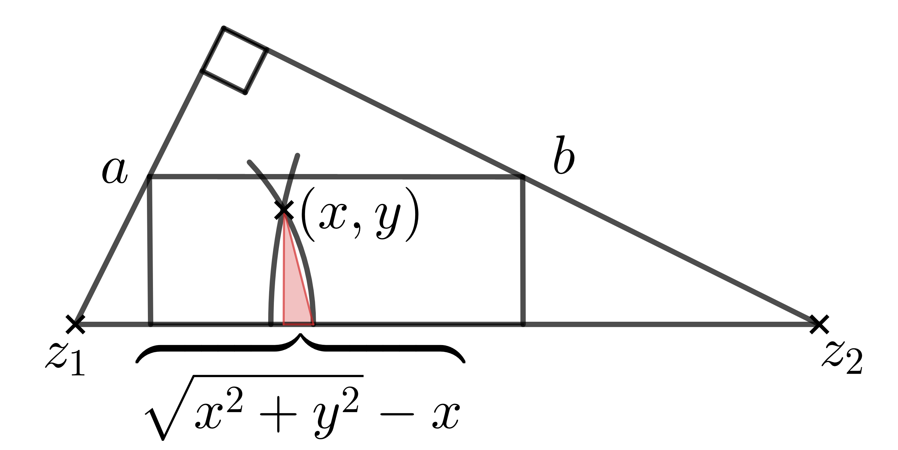
Figure 2. The Cap $J_{a,b}$ (with sides lengths $a,b$ and height $\frac{ab}{\sqrt{a^{2}+b^{2}}}$) and inscribed rectangle $R$ of half the height.

Again, setting $\xi=(x,y)$, we have that

(8) $$\text{vol}(B(z_{1},\xi)\cap B(z_{2},\xi)\cap J_{\delta})\ \geq\ \frac{1}{2}y\cdot(\sqrt{x^{2}+y^{2}}-x)\ \geq\ \frac{y^{3}}{4(x+y)}$$

Combining Lemma 3.3 with inequality (8) gives

(9) $$\Pr[Z(J_{a,b})\ |\ \mkern 1.5mu\overline{\mkern-1.5muJ_{a,b}\mkern-1.5mu}\mkern 1.5mu\ ]\ \geq\ \int_{J_{a,b}}\text{vol}(B(z_{1},\xi)\cap B(z_{2},\xi)\cap J_{a,b})\ d\xi\ \geq\ \int_{J_{a,b}}\frac{y^{3}}{4(x+y)}\ dx\,dy\\$$

Recall the cap $J_{a,b}$ has perpendicular side lengths $a\leq b$. Thus the height of $J_{a,b}$ is $\frac{ab}{\sqrt{a^{2}+b^{2}}}$. Again, a lower bound can be obtained by integrating over an inscribed rectangle rather than over the entire cap $J_{a,b}$. Specifically, let $R$ be the inscribed rectangle with half the height of $J_{a,b}$; see Figure 2. Then

$$\int_{J_{a,b}}\,\frac{y^{3}}{4(x+y)}\ dx\,dy \ \geq\ \int_{R}\,\frac{y^{3}}{4(x+y)}\ dx\,dy$$

$$\ \geq\ \int_{0}^{\frac{ab}{2\sqrt{a^{2}+b^{2}}}}\int_{\frac{a^{2}}{2\sqrt{a^{2}+b^{2}}}}^{\frac{a^{2}}{\sqrt{a^{2}+b^{2}}}+\frac{b^{2}}{2\sqrt{a^{2}+b^{2}}}}\frac{y^{3}}{4(x+y)}\ dx\,dy$$

$$\ =\ \frac{1}{4}\cdot\int_{0}^{\frac{ab}{2\sqrt{a^{2}+b^{2}}}}y^{3}\cdot\Big{[}\ln(x+y)\Big{]}_{\frac{a^{2}}{2\sqrt{a^{2}+b^{2}}}}^{\frac{a^{2}}{\sqrt{a^{2}+b^{2}}}}\ dy$$

$$\ =\ \frac{1}{4}\cdot\int_{0}^{\frac{ab}{2\sqrt{a^{2}+b^{2}}}}y^{3}\cdot\ln\left(\frac{\frac{a^{2}}{\sqrt{a^{2}+b^{2}}}+\frac{b^{2}}{2\sqrt{a^{2}+b^{2}}}+y}{\frac{a^{2}}{2\sqrt{a^{2}+b^{2}}}+y}\right)\,dy$$

$$\ =\ \frac{1}{4}\cdot\int_{0}^{\frac{ab}{2\sqrt{a^{2}+b^{2}}}}y^{3}\cdot\ln\left(1+\frac{a^{2}+b^{2}}{a^{2}+2y\sqrt{a^{2}+b^{2}}}\right)\,dy$$

(10) $$\ \geq\ \frac{1}{4}\cdot\int_{0}^{\frac{ab}{2\sqrt{a^{2}+b^{2}}}}y^{3}\cdot\ln\left(1+\frac{a^{2}+b^{2}}{a^{2}+ab}\right)\,dy$$

To simplify (4.2) recall that $a\leq b$, by assumption. Thus $\frac{b}{\sqrt{a^{2}+b^{2}}}\geq\frac{1}{\sqrt{2}}\geq\frac{1}{2}$. This implies that

$$\int_{J_{a,b}}\,\frac{y^{3}}{4(x+y)}\,dx\,dy \ \geq\ \frac{1}{4}\cdot\int_{0}^{\frac{ab}{2\sqrt{a^{2}+b^{2}}}}y^{3}\cdot\ln\left(1+\frac{a^{2}+b^{2}}{a^{2}+ab}\right)\,dy$$

$$\ \geq\ \frac{1}{8}\cdot\left(1+\ln\left(\frac{b}{a}\right)\right)\cdot\int_{0}^{\frac{ab}{2\sqrt{a^{2}+b^{2}}}}y^{3}\,dy$$

$$\ \geq\ \frac{1}{8}\cdot\left(1+\ln\left(\frac{b}{a}\right)\right)\cdot\int_{0}^{\frac{a}{4}}y^{3}\,dy$$

(11) $$\ =\ \frac{1}{2^{11}}\,a^{4}\cdot\left(1+\ln\left(\frac{b}{a}\right)\right)$$

Here the second inequality arises since

$$\left(1+\frac{a^{2}+b^{2}}{a^{2}+ab}\right)^{2}\ =\ \left(\frac{b}{a}+\frac{2}{\frac{b}{a}+1}\right)^{2}\ \geq\ \left(\frac{b}{a}+\frac{a}{b}\right)^{2}\ \geq\ 2+\left(\frac{b}{a}\right)^{2}\ \geq\ e\cdot\frac{b}{a}$$

Thus, taking the log on both sides gives the second inequality. Putting together inequalities (9) and (4.2) completes the proof. ∎

Theorem 4.4.

For the unit square $\mathbb{H}$, the expected group size after $T$ rounds is $\mathbb{E}[|G^{T}|]\gtrsim\ln(T)$.

Proof.

For each $t$, consider the triangle $A^{t}=\text{conv}\left((0,0),\left(0,\frac{1}{4t^{\frac{1}{4}}}\right),\left(\frac{1}{4t^{\frac{1}{4}}},0\right)\right)$. As discussed, the triangle $A^{t}$ is a cap of the unit square. Observe that,

$$\Pr[X^{t+1}] \ \geq\ \Pr[Z(A^{t})\wedge(S^{t}\cap A^{t}=\emptyset)]$$

$$\ =\ \Pr[Z(A^{t})\ |\ (S^{t}\cap A^{t}=\emptyset)\ ]\cdot\Pr[\ S^{t}\cap A^{t}=\emptyset\ ]$$

$$\ \geq\ \Pr[Z(A^{t})\ |\ \mkern 1.5mu\overline{\mkern-1.5muA^{t}\mkern-1.5mu}\mkern 1.5mu\ ]\cdot\Pr[\ S^{t}\cap A^{t}=\emptyset\ ]$$

(12) $$\ \gtrsim\ \frac{1}{t}\cdot\Pr[\ S^{t}\cap A^{t}=\emptyset\ ]$$

Here the second inequality follows from Corollary 2.2. The third inequality is derived by applying Lemma 4.3 with respect to the cap $A^{t}$, for which $a=b=\frac{1}{4t^{\frac{1}{4}}}$.

Claim 4.5.

There exist constants $c,\tau$ such that $\Pr[\ S^{t}\cap A^{t}=\emptyset\ ]\geq c$ for all $t\geq\tau$

proof of claim.

First we show that there exists constant $\tau$ such that the convex hull $S^{\tau}$ contains the square $Q=\left[\frac{1}{4},\frac{3}{4}\right]^{2}$ with probability bounded below by some positive constant. To see this, let $T_{1},T_{2},T_{3}$ and $T_{4}$ be right-angled triangles each containing one of the corners with perpendicular side lengths $a=b=\frac{1}{4}$. By Lemma 4.3, the probability of accepting a candidate inside triangle $T_{\ell}$, given no member is currently in $T_{\ell}$, is lower bounded by $\frac{a^{4}}{2^{11}}=\frac{1}{2^{19}}$. Hence we have,

(13) $$\Pr[T_{\ell}\cap S^{i}=\emptyset]\ \leq\ \left(1-\frac{1}{2^{19}}\right)^{i}\ =\ k^{i}$$

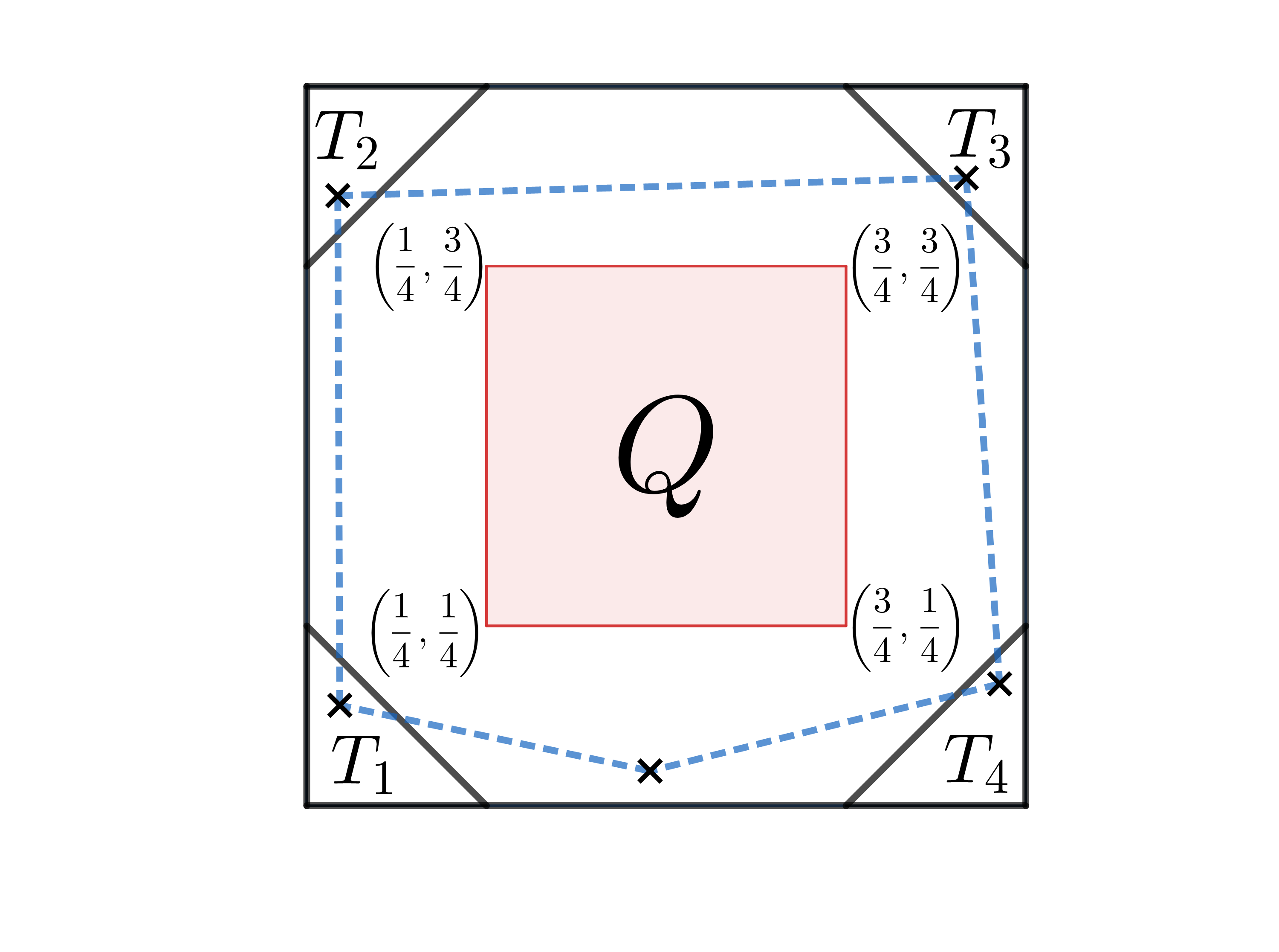
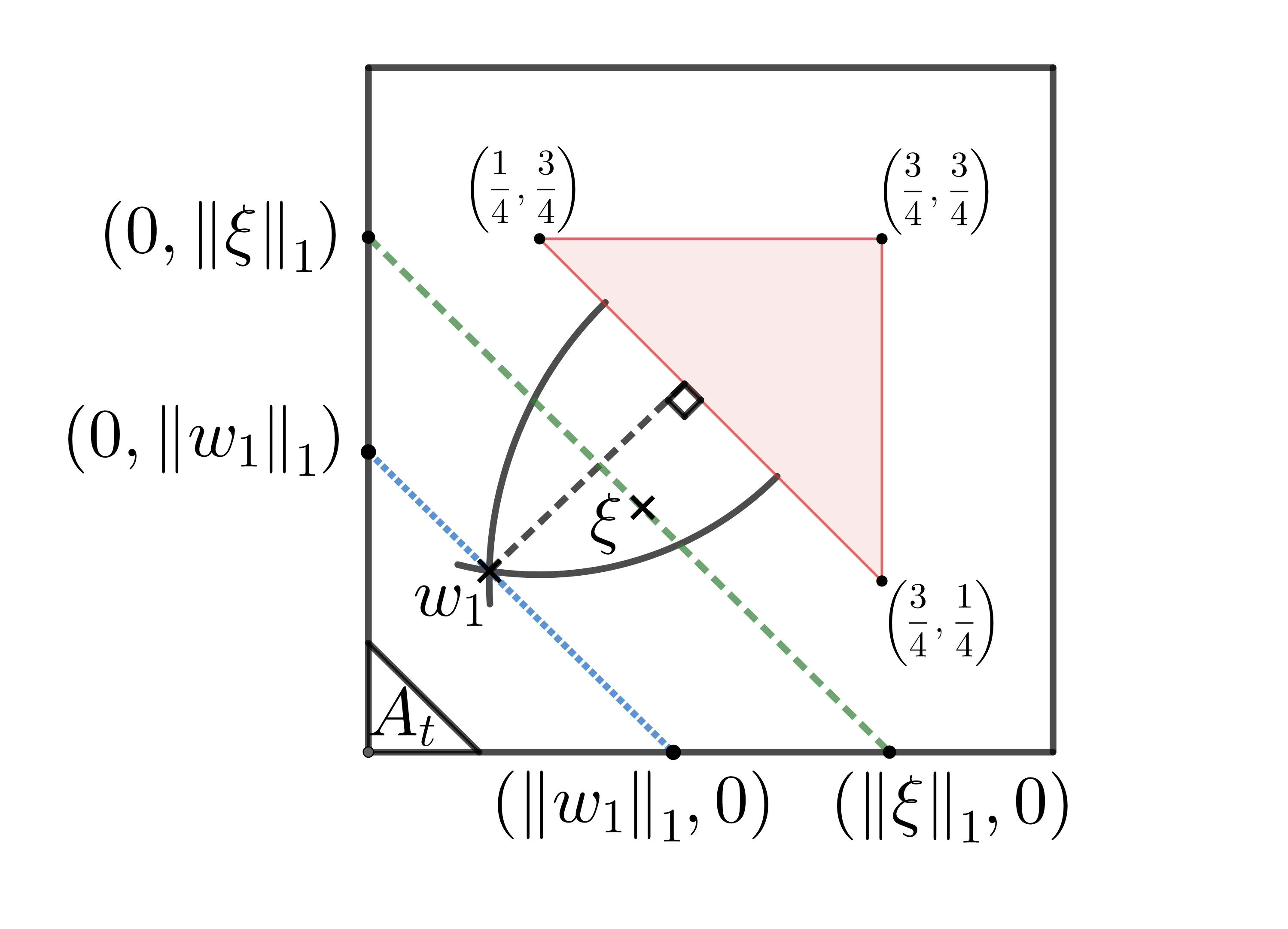
Figure 3. Figure on the left illustrates that if there is a member in each $T_{\ell}$ then $Q\subseteq S_{i}$. The figure on the right shows if $\xi\in B\left(\left(\frac{1}{4},\frac{3}{4}\right),w_{1}\right)\cap B\left(\left(\frac{3}{4},\frac{1}{4}\right),w_{1}\right)$ then $\|\xi\|_{1}\geq\|w_{1}\|_{1}$

Observe that if there is a member of $S^{i}$ selected in each of the four triangles $T_{1},T_{2},T_{3}$ and $T_{4}$ then $Q\subseteq S^{i}$, as illustrated in Figure 3. Consequently, applying the union bound and (13), for all $1\leq\ell\leq 4$, we have $\Pr[Q\not\subseteq S^{i}]\leq 4k^{i}$. Note, since $k=1-\frac{1}{2^{19}}$, there exists a fixed constant $\tau$ such that $4k^{\tau}<1$; hence, $\Pr[Q\subseteq S^{\tau}]\geq 1-4k^{\tau}>0$. Consider any round $t\geq\tau+1$ then,

$$\Pr[\ S^{t}\cap A^{t}=\emptyset\ ] \geq\Pr[\ (S^{t}\cap A^{t}=\emptyset)\wedge(Q\subseteq S^{\tau})\ ]$$

(14) $$=\Pr[\ S^{t}\cap A^{t}=\emptyset\ |\ Q\subseteq S^{\tau}\ ]\Pr[Q\subseteq S^{\tau}]$$

Since we know that $\Pr[Q\subseteq S^{\tau}]$ is bounded below by a constant, we need to show the remaining term of (14) is bounded below by constant. Recursively we have,

$$\Pr[S^{t}\cap A^{t} =\emptyset\ |\ Q\subseteq S^{\tau}\ ]$$

$$\ =\ \Pr[\neg Z(A^{t})\wedge(S^{t-1}\cap A^{t}=\emptyset)\ |\ Q\subseteq S^{\tau}]$$

$$\ =\ \Pr[\neg Z(A^{t})\ |\ (S^{t-1}\cap A^{t}=\emptyset)\wedge(Q\subseteq S^{\tau})]\cdot\Pr[\ S^{t-1}\cap A^{t}=\emptyset\ |Q\subseteq S^{\tau}]$$

$$\ =\ \Pr[\ S^{\tau}\cap A^{t}=\emptyset\ |\ Q\subseteq S^{\tau}]\cdot\prod_{i=\tau}^{t-1}\,(1-\Pr[Z(A^{t})\ |\ S^{i}\cap A^{t}=\emptyset\wedge(Q\subseteq S^{\tau})])$$

$$\ \gtrsim\ \Pr[\ S^{\tau}\cap A^{\tau}=\emptyset\ |\ Q\subseteq S^{\tau}]\cdot\prod_{i=\tau}^{t-1}\,(1-\Pr[Z(A^{t})\ |\ S^{i}\cap A^{t}=\emptyset\wedge(Q\subseteq S^{\tau})])$$

$$\ \gtrsim\ \Pr[\ S^{\tau}\cap A^{\tau}=\emptyset\ |\ Q\subseteq S^{\tau}]\cdot\prod_{i=\tau}^{t-1}\,(1-\Pr[Z(A^{t})\ |\ Q])$$

(15) $$\ \gtrsim\ \prod_{i=\tau}^{t-1}\,(1-\Pr[Z(A^{t})\ |\ Q])$$

Here the first inequality holds because, by definition, $A^{t}\subseteq A^{\tau}$ for all $t\geq\tau+1$. For the second inequality, observe that $S^{\tau}\subseteq S^{i}$ when $i\geq\tau$. Thus, by Corollary 2.2, $\Pr[Z(A^{t})\ |\ S^{i}\cap A^{t}=\emptyset\wedge(Q\subseteq S^{\tau})]\leq\Pr[Z(A^{t})\ |\ Q\ ]$. The last inequality holds because $\tau$ is constant, so $A^{\tau}$ is a small fixed triangle and there is a positive probability that no candidate was selected inside $A^{\tau}$ in the first $\tau$ rounds, even when the convex hull of the members includes the square $Q$.

Next, we claim that if $Q$ is the convex hull then a candidate can be accepted inside $A^{t}$ only if both candidates are in $A^{t}$. In particular, this gives the following useful inequality:

(16) $$\Pr[\ Z(A^{t})\ |\ Q]\ \leq\ \text{vol}(A^{t})^{2}\ =\ \left(\frac{1}{2}\left(\frac{1}{4t^{\frac{1}{4}}}\right)^{2}\right)^{2}\ =\ \frac{1}{2^{10}\cdot t}$$

To see this, suppose the claim is false. That is, $w_{2}\in A^{t}$ is selected when $Q$ is the convex hull but $w_{1}\notin A^{t}$. Then, by Lemma 2.3, it must be the case that

$$w_{2}\in B\left(\left(\frac{1}{4},\frac{1}{4}\right),w_{1}\right)\cap B\left(\left(\frac{3}{4},\frac{1}{4}\right),w_{1}\right)\cap B\left(\left(\frac{1}{4},\frac{3}{4}\right),w_{1}\right)\cap B\left(\left(\frac{3}{4},\frac{3}{4}\right),w_{1}\right)$$

Observe that $w_{1}\in A^{t}$ if and only if $\|w_{1}\|_{1}=|(w_{1})_{1}|+|(w_{1})_{2}|\leq\frac{1}{4t^{\frac{1}{4}}}$, where $(w_{1})_{i}$ denotes the $i$’th component of $w_{1}$. Since $w_{1}\not\in A^{t}$, we have $\|w_{1}\|_{1}>\frac{1}{4t^{\frac{1}{4}}}$. As illustrated in Figure 3, the region $B((\frac{1}{4},\frac{3}{4}),w_{1})\cap B((\frac{3}{4},\frac{1}{4}),w_{1})$ does not intersect $A^{t}$ if $w_{1}\not\in A^{t}$. Thus, the winner $w_{2}$ cannot be inside $A^{t}$ and the claim is verified.

Finally combining (14),(15) and (16), we have for any $t\geq\tau+1$

$$\Pr[S^{t}\cap A^{t}=\emptyset]\gtrsim\prod_{i=\tau}^{t-1}\left(1-\frac{1}{2^{10}\cdot t}\right) \ \gtrsim\ \left(1-\frac{1}{2^{10}\cdot t}\right)^{t}\qed$$

Using the Claim 4.5 and (4.2) we get $\Pr[X^{t+1}]\gtrsim\frac{1}{t}$ for any $t\geq\tau+1$. Ergo, we have  $\mathbb{E}[G^{T}]=\sum_{t=1}^{T}\Pr[X^{t}]\gtrsim\sum_{t=\tau+1}^{T}\frac{1}{t}\cong\ln(T)$. ∎

5. Upper Bounds on Expected Group Size

We now apply the techniques developed in Sections 3 and 4 to upper bound the expected cardinality of the group for the unit ball and the unit square. Specifically, we apply Corollary 3.2 to these metric spaces using the $f_{K}$ obtained from Lemma 4.1 and Lemma 4.3, respectively.

5.1. Upper Bound for the Unit Ball

Observe that exactly one of the two Voronoi regions corresponds to a circular segment. Furthermore, since a circular segment fits inside its complement, $\arg\min\limits_{i}\Pr[Z(H_{i}(w_{1},w_{2}))|\mkern 1.5mu\overline{\mkern-1.5muH_{i}(w_{1},w_{2})\mkern-1.5mu}\mkern 1.5mu]$ is attained by the $H_{i}$ corresponding to a circular segment. Let $\delta(w_{1},w_{2})$ denote the height of the circular segment for this Voronoi region $H_{i}$. Then, by Lemma 4.1, we have $\min\limits_{i}\Pr[\ Z(H_{i}(w_{1},w_{2}))\ |\ \mkern 1.5mu\overline{\mkern-1.5muH_{i}(w_{1},w_{2})\mkern-1.5mu}\mkern 1.5mu\ ]\gtrsim\delta(w_{1},w_{2})^{4}$. Thus $f_{\mathbb{B}}(w_{1},w_{2})=\delta(w_{1},w_{2})^{4}$, satisfies the conditions of Corollary 3.2. However when using Corollary 3.2 we need to understand $\Phi(\lambda)$; Lemma 5.1 allows us to do exactly that.

Lemma 5.1.

Let $\delta(w_{1},w_{2})$ be the height of the circular segment $H_{i}(w_{1},w_{2})$ formed by the Voronoi regions. Then, for all $\lambda\leq\frac{1}{10^{4}}$, we have

$$\Phi(\lambda)\ =\ \int\int\mathbb{I}\left[\delta(w_{1},w_{2})^{4}\leq\lambda\right]\,dw_{1}\,dw_{2}\ \lesssim\ \lambda^{\frac{7}{8}}$$

Proof of Lemma 5.1.

Let $\mathcal{H}$ be the hyperplane separating the two Voronoi regions. Since $\mathcal{H}$ contains the midpoint $\frac{1}{2}(w_{2}+w_{1})$ and has normal vector $w_{2}-w_{1}$, it holds that

(17) $$\mathcal{H}(w_{1},w_{2}) =\Big{\{}\xi\in\mathbb{R}^{2}\ :\ (w_{2}-w_{1})\cdot\left(\xi-\frac{w_{2}+w_{1}}{2}\right)=0\Big{\}}$$

By basic algebra, the distance from the origin to $\mathcal{H}$ is $\frac{|\|w_{2}\|^{2}-\|w_{1}\|^{2}|}{2\sqrt{(w_{2}-w_{1})^{2}_{2}+(w_{2}-w_{1})^{2}_{1}}}$. Hence we have,

(18) $$\delta(w_{1},w_{2})=1-\left(\frac{|\|w_{2}\|^{2}-\|w_{1}\|^{2}|}{2\sqrt{(w_{2}-w_{1})^{2}_{2}+(w_{2}-w_{1})^{2}_{1}}}\right)$$

Note that $\delta(w_{1},w_{2})=\delta(w_{2},w_{1})$ because swapping positions of the candidates does not change the sizes of Voronoi regions. It will now be convenient to work with polar coordinates. So denote $w_{1}=(r,\varphi)$ and $w_{2}=(\xi,\theta)$. Observe that

$$\Phi(\lambda) \ =\ \int\int\mathbb{I}\left[\delta(w_{1},w_{2})\leq\lambda^{\frac{1}{4}}\right]\,dw_{2}\,dw_{1}$$

$$\ =\ 2\int\int\mathbb{I}\left[\delta(w_{1},w_{2})\leq\lambda^{\frac{1}{4}},\|w_{1}\|\leq\|w_{2}\|\right]\,dw_{2}\,dw_{1}$$

$$\ =\ 2\int_{-\pi}^{\pi}\int_{0}^{1}\int\mathbb{I}\left[\delta((r,\varphi),w_{2})\leq\lambda^{\frac{1}{4}},r\leq\|w_{2}\|\right]\,dw_{2}\,r\,dr\,d\varphi$$

$$\ =\ 4\pi\int_{0}^{1}\int\mathbb{I}\left[\delta((r,0),w_{2})\leq\lambda^{\frac{1}{4}},r\leq\|w_{2}\|\right]\,dw_{2}\,r\,dr$$

$$\ =\ 4\pi\int_{0}^{1}\int_{r}^{1}\int_{-\pi}^{\pi}\mathbb{I}\left[\delta((r,0),(\xi,\theta))\leq\lambda^{\frac{1}{4}}\right]\,\xi\,d\theta\,d\xi\,r\,dr$$

$$\ \leq\ 4\pi\int_{0}^{1}\int_{r}^{1}\int_{-\pi}^{\pi}\mathbb{I}\left[\delta((r,0),(1,\theta))\leq\lambda^{\frac{1}{4}}\right]\,\xi\,d\theta\,d\xi\,r\,dr$$

(19) $$\ =\ 4\pi\int_{0}^{1}\int_{-\pi}^{\pi}\mathbb{I}\left[\delta((r,0),(1,\theta))\leq\lambda^{\frac{1}{4}}\right]\left(\frac{1-r^{2}}{2}\right)\,r\,d\theta\,dr$$

The first equality follows as $\delta(w_{1},w_{2})=\delta(w_{2},w_{1})$. The fourth equality holds by rotational symmetry. The inequality holds because, by equation (18), we have

$$\delta((r,0),(\xi,\theta)) \ =\ 1-\left(\frac{\xi^{2}-r^{2}}{2}\right)\frac{1}{\sqrt{\xi^{2}\sin^{2}(\theta)+(\xi\cos(\theta)-r)^{2}}}$$

$$\ =\ 1-\left(\frac{\xi^{2}-r^{2}}{2}\right)\frac{1}{\sqrt{\xi^{2}+r^{2}-2r\xi\cos(\theta)}}$$

$$\ \geq\ 1-\left(\frac{1-r^{2}}{2}\right)\frac{1}{\sqrt{1+r^{2}-2r\cos(\theta)}}$$

$$\ =\ \delta((r,0),(1,\theta))$$

Note that if $r<1-2\lambda^{\frac{1}{4}}$ then we have $\delta((r,0),(1,\theta))\geq\delta((r,0),(1,0))=\frac{1-r}{2}>\lambda^{\frac{1}{4}}$. Hence we see

$$\int_{0}^{1}\int_{-\pi}^{\pi}\mathbb{I} \left[\delta((r,0),(1,\theta))\leq\lambda^{\frac{1}{4}}\right]\left(\frac{1-r^{2}}{2}\right)\,r\,d\theta\,dr$$

$$\ =\ \int_{1-2\lambda^{\frac{1}{4}}}^{1}\int_{-\pi}^{\pi}\mathbb{I}\left[\delta((r,0),(1,\theta))\leq\lambda^{\frac{1}{4}}\right]\left(\frac{1-r^{2}}{2}\right)\,r\,d\theta\,dr$$

(20) $$\ \lesssim\ \lambda^{\frac{1}{2}}\max\limits_{r\in[1-2\lambda^{\frac{1}{4}},1]}\int_{-\pi}^{\pi}\mathbb{I}\left[\delta((r,0),(1,\theta))\leq\lambda^{\frac{1}{4}}\right]d\theta$$

Here the last inequality hold as $\int_{1-2\lambda^{\frac{1}{4}}}^{1}\left(\frac{1-r^{2}}{2}\right)rdr\leq\int_{1-2\lambda^{\frac{1}{4}}}^{1}\left(1-r\right)dr=2\lambda^{\frac{1}{2}}$. Finally, note that

$$\max\limits_{r\in[1-2\lambda^{\frac{1}{4}},1]}\ \int_{-\pi}^{\pi}\mathbb{I}\left[\delta((r,0),(1,\theta))\leq\lambda^{\frac{1}{4}}\right]\,d\theta$$

$$\ =\ \max\limits_{r\in[1-2\lambda^{\frac{1}{4}},1]}\int_{-\pi}^{\pi}\mathbb{I}\left[1-\left(\frac{1-r^{2}}{2}\right)\frac{1}{\sqrt{1+r^{2}-2r\cos(\theta)}}\leq\lambda^{\frac{1}{4}}\right]\,d\theta$$

$$\ \leq\ \max\limits_{r\in[1-2\lambda^{\frac{1}{4}},1]}\int_{-\pi}^{\pi}\mathbb{I}\left[1-\left(\frac{1-r^{2}}{2}\right)\frac{1}{\sqrt{1+r^{2}-2r(1-\frac{\theta^{2}}{8})}}\leq\lambda^{\frac{1}{4}}\right]\,d\theta$$

$$\ =\ \max\limits_{r\in[1-2\lambda^{\frac{1}{4}},1]}\int_{-\pi}^{\pi}\mathbb{I}\left[\sqrt{1+r^{2}-2r(1-\frac{\theta^{2}}{8})}\leq\frac{1-r^{2}}{2(1-\lambda^{\frac{1}{4}})}\right]\,d\theta$$

$$\ =\ \max\limits_{r\in[1-2\lambda^{\frac{1}{4}},1]}\int_{-\pi}^{\pi}\mathbb{I}\left[\sqrt{(1-r)^{2}+\frac{r\theta^{2}}{4}}\leq\frac{1-r^{2}}{2(1-\lambda^{\frac{1}{4}})}\right]\,d\theta$$

(21) $$\ =\ \max\limits_{r\in[1-2\lambda^{\frac{1}{4}},1]}\int_{-\pi}^{\pi}\mathbb{I}\left[\sqrt{1+\frac{r\theta^{2}}{4(1-r)^{2}}}\leq\frac{1+r}{2(1-\lambda^{\frac{1}{4}})}\right]\,d\theta$$

Now, if $|\theta|\geq 8\lambda^{\frac{3}{8}}$ then for any $r\in[1-2\lambda^{\frac{1}{4}},1]$, we have

$$\sqrt{1+\frac{r\theta^{2}}{4(1-r)^{2}}}-\frac{1+r}{2(1-\lambda^{\frac{1}{4}})} \ \geq\ \sqrt{1+\frac{16r\lambda^{\frac{3}{4}}}{(1-r)^{2}}}-\frac{1+r}{2(1-\lambda^{\frac{1}{4}})}$$

$$\ \geq\ \sqrt{1+\frac{16r\lambda^{\frac{3}{4}}}{4\lambda^{\frac{1}{2}}}}-\frac{1+r}{2(1-\lambda^{\frac{1}{4}})}$$

$$\ \geq\ \sqrt{1+4r\lambda^{\frac{1}{4}}}-\frac{1}{(1-\lambda^{\frac{1}{4}})}$$

$$\ \geq\ \sqrt{1+4(1-2\lambda^{\frac{1}{4}})\lambda^{\frac{1}{4}}}-\frac{1}{(1-\lambda^{\frac{1}{4}})}$$

$$\ >\ 0$$

Here the last inequality holds for any $\lambda^{\frac{1}{4}}\leq\frac{1}{10}$. Hence,

$$\max\limits_{r\in[1-2\lambda^{\frac{1}{4}},1]} \int_{-\pi}^{\pi}\mathbb{I}\left[\sqrt{1+\frac{r\theta^{2}}{4(1-r)^{2}}}\leq\frac{1+r}{2(1-\lambda^{\frac{1}{4}})}\right]d\theta$$

$$\leq\max\limits_{r\in[1-2\lambda^{\frac{1}{4}},1]}\int_{-8\lambda^{\frac{3}{8}}}^{8\lambda^{\frac{3}{8}}}\mathbb{I}\left[\sqrt{1+\frac{r\theta^{2}}{4(1-r)^{2}}}\leq\frac{1+r}{2(1-\lambda^{\frac{1}{4}})}\right]d\theta$$

(22) $$\leq 16\lambda^{\frac{3}{8}}$$

Finally, combining (5.1), (5.1), (5.1) and (22), we have, for all $\lambda^{\frac{1}{4}}\leq 0.1$, that

$$\Phi(\lambda) \ \lesssim\ \lambda^{\frac{1}{2}}\cdot\lambda^{\frac{3}{8}}\ =\ \lambda^{\frac{7}{8}}\qed$$

Theorem 5.2.

For the unit ball $\mathbb{B}$, the expected group size after $T$ rounds is $\mathbb{E}[|G^{T}|]\lesssim T^{\frac{1}{8}}$.

Proof.

Let $t_{0}$ be a constant such that such that $\frac{\ln(t_{0})}{t_{0}}\leq\frac{1}{10^{4}}$, then for any round $t\geq t_{0}$ we have $0\leq\lambda\leq\frac{\ln(t)}{t}\leq\frac{\ln(t_{0})}{t_{0}}\leq\frac{1}{10^{4}}$. Thus applying Corollary 3.2 along with Lemma 5.1 for $t\geq t_{0}$, we see that

$$\Pr[X^{t+1}]\lesssim\frac{1}{t}+\int_{0}^{\frac{\ln(t)}{t}}te^{-t\lambda}\lambda^{\frac{7}{8}}d\lambda=\frac{1}{t}+\frac{1}{t^{\frac{7}{8}}}\int_{0}^{\ln(t)}e^{-u}\cdot u^{\frac{7}{8}}du\lesssim\frac{1}{t^{\frac{7}{8}}}$$

Here the equality holds by the substitution $u=t\lambda$. The last inequality holds since

$$\int_{0}^{\ln(t)}e^{-u}u^{\frac{7}{8}}\,du\ \leq\ 1+\int_{1}^{\infty}e^{-u}u\,du\ \leq\ 2$$

The theorem follows as $\mathbb{E}[|G^{T}|]=\sum_{t=1}^{T}\Pr[X^{t}]\lesssim t_{0}+\sum_{t=t_{0}+1}^{T}1/t^{\frac{7}{8}}\lesssim T^{\frac{1}{8}}$ by applying integral bounds. ∎

5.2. Upper Bound for the Unit Square

Similar to the unit ball case, we must find an appropriate function $f_{\mathbb{H}}$ satisfying the conditions of Corollary 3.2. For a cap $A$ with $A\subseteq H_{i}(w_{1},w_{2})$ by Corollary 2.2,

(23) $$\Pr[\ Z(H_{i}(w_{1},w_{2}))\ |\ \mkern 1.5mu\overline{\mkern-1.5muH_{i}(w_{1},w_{2})\mkern-1.5mu}\mkern 1.5mu\ ]\geq\Pr[\ Z(A)\ |\ \mkern 1.5mu\overline{\mkern-1.5muH_{i}(w_{1},w_{2})\mkern-1.5mu}\mkern 1.5mu\ ]\geq\Pr[\ Z(A)\ |\ \mkern 1.5mu\overline{\mkern-1.5muA\mkern-1.5mu}\mkern 1.5mu\ ]$$

Let $a(w_{1},w_{2})\leq b(w_{1},w_{2})$ be the two side lengths of the triangular cap of greatest area that fits inside both $H_{i}(w_{1},w_{2})$. Applying Lemma 4.3, along with (23) gives

$$\min\limits_{i}\Pr[\ Z(H_{i}(w_{1},w_{2}))\ |\ \mkern 1.5mu\overline{\mkern-1.5muH_{i}(w_{1},w_{2})\mkern-1.5mu}\mkern 1.5mu\ ]\ \gtrsim\ a(w_{1},w_{2})^{4}\cdot\ln\left(e\cdot\frac{b(w_{1},w_{2})}{a(w_{1},w_{2})}\right)$$

Thus $f_{\mathbb{H}}(w_{1},w_{2})=a(w_{1},w_{2})^{4}\ln\left(e\frac{b(w_{1},w_{2})}{a(w_{1},w_{2})}\right)$ satisfies the conditions of Corollary 3.2.

Lemma 5.3.

Let $a(w_{1},w_{2})\leq b(w_{1},w_{2})$ be the two side lengths of the triangular cap of greatest area that fits inside both $H_{i}(w_{1},w_{2})$. Then, for any $\lambda\leq\frac{1}{20}$,

$$\Phi(\lambda)\ =\ \int\int\mathbb{I}\left[a(w_{1},w_{2})^{4}\cdot\ln\left(e\cdot\frac{b(w_{1},w_{2})}{a(w_{1},w_{2})}\right)\leq\lambda\right]\,dw_{1}\,dw_{2}\ \lesssim\ \lambda\cdot\ln\left(\ln\left(\frac{1}{\lambda}\right)\right)$$

Proof.

We need only consider pairs $w_{1}$ and $w_{2}$ that satisfy the indicator function. As $\lambda\leq\frac{1}{20}$, this implies $a(w_{1},w_{2})\leq\lambda^{\frac{1}{4}}\leq\left(\frac{1}{20}\right)^{\frac{1}{4}}\leq\frac{1}{2}$ and, without loss of generality, $H_{1}(w_{1},w_{2})$ is the smallest Voronoi region and fits (under symmetries) into $H_{2}(w_{1},w_{2})$. Furthermore, applying rotational and diagonal symmetries, any pair of points can be transformed into a pair of the form $w_{1}=(x,y)$ and $w_{2}=(x+\Delta_{x},y+\Delta_{y})$, with $s=\Delta_{y}/\Delta_{x}\leq 1$ and $\Delta_{x},\Delta_{y}\geq 0$. Hence, we lose only a constant factor in making the following assumptions on $w_{1}$ and $w_{2}$: the triangular cap of greatest area that fits inside both the $H_{i}(w_{1},w_{2})$ is contained in $H_{1}(w_{1},w_{2})$; the cap contains the origin; the larger side corresponding to $b(w_{1},w_{2})$ is along the $y$-axis; the smaller side corresponding to $a(w_{1},w_{2})$ is along the $x$-axis.

Recall that $H_{1}(w_{1},w_{2})$ is either a right-angled triangle or a right-angled trapezoid. In the former case, the triangular cap of greatest area which fits inside both of the Voronoi regions is $H_{1}$ itself. The side lengths of $H_{1}$ are then the intercepts of $\mathcal{H}$ along the axes, where $\mathcal{H}$ is the hyperplane separating the two Voronoi regions. In the latter case, the triangular cap of greatest area satisfies $b(w_{1},w_{2})=1$ and $a(w_{1},w_{2})$ is the intercept of $\mathcal{H}$ on the $x$-axis. We can then compute explicit expressions for both terms $a(w_{1},w_{2})$ and $b(w_{1},w_{2})$. In particular,

(24) $$a(w_{1},w_{2})=\frac{\|w_{2}\|^{2}-\|w_{1}\|^{2}}{2(w_{2}-w_{1})_{1}}=x+sy+\frac{\Delta_{x}}{2}(1+s^{2})=x+sy+\frac{\Delta_{y}}{2}\left(\frac{1+s^{2}}{s}\right)$$

The first equality holds by definition (17) of hyperplane $\mathcal{H}$. Now, because this is the unit square, we have $b(w_{1},w_{2})\leq 1$. Thus, $b(w_{1},w_{2})=\min\left(1,\frac{a(w_{1},w_{2})}{s}\right)$. Hence,

(25) $$a(w_{1},w_{2})^{4}\ln\left(e\cdot\frac{b(w_{1},w_{2})}{a(w_{1},w_{2})}\right)\ =\ a(w_{1},w_{2})^{4}\ln\left(e\min\left(\frac{1}{a(w_{1},w_{2})},\frac{1}{s}\right)\right)$$

For a fixed $w_{1}=(x,y)$, let $R(x,y)$ be a rectangle containing all the points $w_{2}=(x+\Delta_{x},y+\Delta_{y})$ satisfying the condition of the indicator function. Thus, it will suffice to show that we can select $R(x,y)$ to have small area. To do this we must show that $\Delta_{x}$ and $\Delta_{y}$ cannot be too large. Again, recall that if the indicator function is true then $a(w_{1},w_{2})\leq\lambda^{\frac{1}{4}}$. So (24) implies $x\leq\lambda^{\frac{1}{4}}$ and $s\leq\frac{\lambda^{\frac{1}{4}}}{y}$. If $\lambda^{\frac{1}{4}}\leq y\leq 1$ then $\min\left(\frac{1}{a(w_{1},w_{2})},\frac{1}{s}\right)\geq\frac{y}{\lambda^{\frac{1}{4}}}$. Plugging into (25) gives $a(w_{1},w_{2})^{4}\cdot\ln\left(e\cdot\frac{b(w_{1},w_{2})}{a(w_{1},w_{2})}\right)\geq a(w_{1},w_{2})^{4}\cdot\ln\left(e\cdot\frac{y}{\lambda^{\frac{1}{4}}}\right)$. It follows that $a(w_{1},w_{2})\leq\frac{\lambda^{1/4}}{\ln^{1/4}\left(\frac{ey}{\lambda^{1/4}}\right)}$. Therefore, (24) gives:

(26) $$\Delta_{x} \ \leq\ 2\cdot\left(\frac{\lambda^{\frac{1}{4}}}{\ln^{\frac{1}{4}}\left(\frac{ey}{\lambda^{\frac{1}{4}}}\right)}-ys-x\right)\ \ \ \leq\ 2\cdot\left(\frac{\lambda^{\frac{1}{4}}}{\ln^{\frac{1}{4}}\left(\frac{ey}{\lambda^{\frac{1}{4}}}\right)}-x\right)$$

(27) $$\Delta_{y} \ \leq\ 2s\cdot\left(\frac{\lambda^{\frac{1}{4}}}{\ln^{\frac{1}{4}}\left(\frac{ey}{\lambda^{\frac{1}{4}}}\right)}-ys-x\right)\ \leq\ \frac{1}{2y}\cdot\left(\frac{\lambda^{\frac{1}{4}}}{\ln^{\frac{1}{4}}\left(\frac{ey}{\lambda^{\frac{1}{4}}}\right)}-x\right)^{2}$$

The final inequalities in (26) and (27) were obtained by optimizing over $s\in[0,1]$. Then noting that $x\leq\lambda^{\frac{1}{4}}$, we have

$$\Phi(\lambda) \ \lesssim\ \int_{0}^{1}\int_{0}^{\lambda^{\frac{1}{4}}}|R(x,y)|\,dx\,dy$$

$$\ =\ \int_{0}^{\lambda^{\frac{1}{4}}}\int_{0}^{\lambda^{\frac{1}{4}}}|R(x,y)|\,dx\,dy+\int_{\lambda^{\frac{1}{4}}}^{1}\int_{0}^{\lambda^{\frac{1}{4}}}|R(x,y)|\,dx\,dy$$

$$\ \lesssim\ \lambda+\int_{\lambda^{1/4}}^{1}\frac{1}{y}\cdot\int_{0}^{\frac{\lambda^{1/4}}{\ln^{1/4}(\frac{ey}{\lambda^{1/4}})}}\,\left(\frac{\lambda^{1/4}}{\ln^{1/4}(\frac{ey}{\lambda^{1/4}})}-x\right)^{3}\,dx\,dy$$

$$\ \lesssim\ \lambda\cdot\int_{\lambda^{1/4}}^{1}\frac{1}{y}\cdot\frac{1}{\ln(\frac{ey}{\lambda^{1/4}})}\,dy$$

$$\ \lesssim\ \lambda\cdot\ln\left(\ln\left(\frac{1}{\lambda}\right)\right)$$

For the second inequality, since $\Delta_{x}$ must be positive, (26) implies that the limit of the integral becomes $x=\frac{\lambda^{1/4}}{\ln^{1/4}(\frac{ey}{\lambda^{1/4}})}$. To bound the area $|R(x,y)|$ of the rectangles we have two cases. When $0\leq y\leq\lambda^{\frac{1}{4}}$, observe, by (24), that $a(w_{1},w_{2})\leq\lambda^{\frac{1}{4}}$ implies $\Delta_{x}\leq 2\lambda^{\frac{1}{4}}$ and $\Delta_{y}\leq 2\lambda^{\frac{1}{4}}$. Thus $|R(x,y)|\leq\Delta_{x}\cdot\Delta_{y}\lesssim\sqrt{\lambda}$. When $\lambda^{\frac{1}{4}}\leq y\leq 1$, the bound on $|R(x,y)|$ holds by (26) and (27). ∎

Theorem 5.4.

For the unit square $\mathbb{H}$, the expected group size after $T$ rounds is

$$\mathbb{E}[|G^{T}|]\lesssim\ln T\cdot\ln\ln T$$

Proof.

Note that for any round $t\geq 100$ we have $0\leq\lambda\leq\frac{\ln(t)}{t}\leq\frac{1}{20}$. Thus, combining Corollary 3.2 and Lemma 5.3 we get

$$\Pr[X^{t+1}] \ \lesssim\ \frac{1}{t}+\int_{0}^{\frac{\ln(t)}{t}}te^{-t\lambda}\cdot\lambda\ln\left(\ln\left(\frac{1}{\lambda}\right)\right)\,d\lambda$$

$$\ =\ \frac{1}{t}+\frac{1}{t}\int_{0}^{1}u\ln\left(\ln\left(\frac{t}{u}\right)\right)du+\frac{1}{t}\int_{1}^{\ln(t)}ue^{-u}\ln\left(\ln\left(\frac{t}{u}\right)\right)du$$

Here the equality holds via the substitution $u=t\lambda$. Note that $u\ln\left(\ln\left(\frac{t}{u}\right)\right)\leq\ln\ln t$, when $t\geq 100$ and $0\leq u\leq 1$. Furthermore,

$$\int_{1}^{\ln(t)}ue^{-u}\cdot\ln\left(\ln\left(\frac{t}{u}\right)\right)\,du\ \leq\ \ln\ln t\cdot\int_{1}^{\infty}ue^{-u}\,du\ \leq\ \ln\ln t$$

Hence it follows $\Pr[X^{t+1}]\lesssim\frac{\ln\ln t}{t}$ for all $t\geq 100$. Finally, we see that $\mathbb{E}[|G^{T}|]=\sum_{t=1}^{T}\Pr[X^{t}]\lesssim 100+\sum_{t=101}^{T}\frac{\ln\ln t}{t}\lesssim\ln T\cdot\ln\ln T$, where the last inequality was obtained using integral bounds. ∎

6. Conclusion

In this paper we presented techniques for studying the evolution of an exclusive social group in a metric space, under the consensus voting mechanism. A natural open problem is to close the gap between the $\Omega(\ln T)$ lower bound and the $O(\ln T\cdot\ln\ln T)$ upper bound on the expected cardinality of the group, after $T$ rounds, in the unit square. Interesting further directions include the study of higher dimensional metric spaces, and allowing for more than two candidates per round. In either direction, our analytic tools may prove useful.

References

- [1] N. Alon, M. Feldman, Y. Mansour, S. Oren, and M. Tennenholtz. Dynamics of evolving social groups. ACM Transactions on Economics and Computation, 7(3):#14, 2019.
- [2] E. Anshelevitch, O. Bhardwaj, and J. Postl. Approximating optimal social choice under metric preferences. In Proceedings of the 29th Conference on Artificial Intelligence (AAAI), pages 777–783, 2015.
- [3] E. Anshelevitch and J. Postl. Randomized social choice functions under metric preferences. Journal of Artificial Intelligence Research, 58(1):797–827, 2017.
- [4] A. Baddeley, I. Bárány, and R. Schneider. Random polytopes, convex bodies, and approximation. In Weil. W, editor, Stochastic Geometry, pages 77–118. Springer, 2007.
- [5] D. Black. On the rationale of group decision-making. Journal of Political Economy, 56:23–34, 1948.
- [6] A. Borodin, O. Lev, N. Shah, and T. Strangway. Primarily about primaries. In Proceedings of the 33rd Conference on Artificial Intelligence (AAAI), pages 1804–1811, 2019.
- [7] R. Claassen. Direction versus proximity: Amassing experimental evidence. American Politics Research, 37(2):227–253, 2009.
- [8] J. Colomer. On the geometry of unanimity rule. Journal of Theoretical Politics, 11(4):543–553, 1999.
- [9] O. Davis, M. Hinich, and P. Ordeshook. An expository development of a mathematical model of the electoral process. American Political Science Review, 64:426–448, 1970.
- [10] A. Downs. An Economic Theory of Democracy. Harper Collins, 1957.
- [11] J. Enelow and M. Hinich. The spatial theory of voting: An introduction. Cambridge University Press, 1984.
- [12] J. Enelow and M. Hinich, editors. Advances in the spatial theory of voting. Cambridge University Press, 1990.
- [13] M. Feldman, A. Fiat, and I. Golomb. On voting and facility location. In Proceedings of 17th Conference on Economics and Computation (EC), pages 269–286, 2016.
- [14] B. Grofman. The neglected role of the status quo in models of issue voting. The Journal of Politics, 47:230–237, 1985.
- [15] P. Hare. Group decision by consensus: Reaching unity in the society of friends. Sociological Inquiry, 43(1):75–84, 1973.
- [16] H. Hotelling. Stability in competition. Economic Journal, 39(153):41–57, 1929.
- [17] D. Lacy and P. Paolino. Testing proximity versus directional voting using experiments. Electoral Studies, 29(3):460–471, 2010.
- [18] J. Lewis and G. King. No evidence on directional vs. proximity voting. Politics Analysis, 8(1):21–33, 2000.
- [19] S. Matthews. A simple direction model of electoral competition. Public Choice, 34:141–156, 1979.
- [20] S. Merrill III, S. Merrill, and B. Grofman. A unified theory of voting: Directional and proximity spatial models. Cambridge University Press, 1999.
- [21] K. Poole. Spatial models of parliamentary voting. Cambridge University Press, 2005.
- [22] G. Rabinowitz and E. Stuart. A directional theory of issue voting. American Political Science Review, 83:93–121, 1989.
- [23] N. Schofield. The spatial models of politics. Routledge, 2007.
- [24] P. Skowron and E. Elkind. Social choice under metric preferences: Scoring rules and STV. In Proceedings of the 31st Conference on Artificial Intelligence (AAAI), pages 706–712, 2017.
- [25] M. Tomz and R. Van Houweling. Candidate position and voter choice. American Political Science Review, 102(3):303–318, 2008.
- [26] E. Vogel, editor. Modern Japanese organization and decision-making. University of California Press, 1975.