CRUDE: Calibrating Regression Uncertainty Distributions Empirically

Abstract

Calibrated uncertainty estimates in machine learning are crucial to many fields such as autonomous vehicles, medicine, and weather and climate forecasting. While there is extensive literature on uncertainty calibration for classification, the classification findings do not always translate to regression. As a result, modern models for predicting uncertainty in regression settings typically produce uncalibrated and overconfident estimates. To address these gaps, we present a calibration method for regression settings that does not assume a particular uncertainty distribution over the error: Calibrating Regression Uncertainty Distributions Empirically (CRUDE). CRUDE makes the weaker assumption that error distributions have a constant arbitrary shape across the output space, shifted by predicted mean and scaled by predicted standard deviation. We detail a theoretical connection between CRUDE and conformal inference. Across an extensive set of regression tasks, CRUDE demonstrates consistently sharper, better calibrated, and more accurate uncertainty estimates than state-of-the-art techniques.

Stanford University
{ezelikman, cjhealy, sharonz, avati}@cs.stanford.edu

1 Introduction

Uncertainty estimates are important across a wide range of applications, from medical diagnosis to weather forecasting to autonomous driving [Leibig et al., 2017, Scher and Messori, 2018, Carvalho et al., 2015]. Accurately assessing the confidence of a prediction, and specifying the underlying distribution of potential errors, is a cornerstone of reliable and interpretable models. For example, having good prediction intervals when forecasting solar power production allows utilities to better account for fluctuations [Murata et al., 2018]. Similarly, having reliable uncertainty estimates on a model assessing tumor size is important, as those metrics may be used to assess a variety of other clinical aspects [Kourou et al., 2015].

While uncertainty calibration for classification is a fairly well-developed research area, uncertainty calibration for regression has remained less explored and the techniques do not readily transfer [Kuleshov et al., 2018]. Notably, previous work has indicated that the models which perform best on the regression tasks they are trained on will rarely be calibrated, and early stopping to guarantee calibration on a calibration dataset will usually hinder model performance overall [Laves et al., 2020].

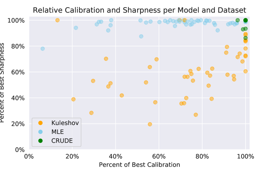
Figure 1: Comparison of calibration techniques, including CRUDE, a Gaussian MLE based on Levi et al. [2019], and the Kuleshov et al. [2018] method. Each point corresponds to the scores of a calibration technique on a particular machine learning model and UCI dataset. This figure visualizes each model’s score relative to the best score on the dataset, so higher values correspond to better performance.

Broadly, there is a trade-off discussed in the literature: some papers, like Kuleshov et al. [2018], exclusively emphasize the calibration performance of calibration methods to produce well-calibrated uncertainty estimates, with little emphasis on the sharpness of the resulting methods. On the other hand, papers such as Levi et al. [2019] emphasize simpler calibration techniques, trading some amount of calibration for a sharper model.

By generalizing key theoretical insights of Kuleshov et al. [2018], Levi et al. [2019], and conformal inference methods [Barber et al., 2021], CRUDE recalibrates by leveraging the empirical distribution of prediction errors measured against a hold-out calibration set. This empirical distribution of errors then defines the shape a family of distributions parameterized by a shift and scale value, which are obtained from the underlying model for each new prediction. We demonstrate, across a wide variety of datasets and models, that it is possible to have both state-of-the-art calibration and sharpness using CRUDE.

Contribution: We propose a calibration method, Calibrating Regression Uncertainty Distributions Empirically (CRUDE), inspired by prior work [Levi et al., 2019, Kuleshov et al., 2018, Barber et al., 2021]. CRUDE assumes less about the underlying error distribution and does not require an auxiliary calibration model, improving calibration and sharpness over both the Levi et al. and Kuleshov et al. approaches on many datasets. Moreover, we demonstrate that this approach substantially improves the calibration of state-of-the-art probabilistic models for object detection. Furthermore, we demonstrate a direct mathematical equivalence with conformal inference, linking these two previously distinct approaches to accurate uncertainty estimates.

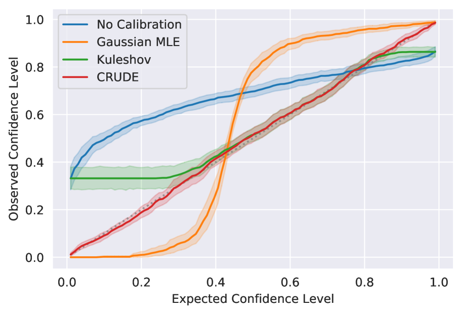
Figure 2: The calibration curves for calibrations of a neural network with a Monte Carlo dropout-derived uncertainty estimate. We show CRUDE, Kuleshov et al., and a Gaussian MLE based on Levi et al., on the Forest Fires dataset [Cortez and Morais, 2007]. Note the ideal calibration curve is the line $x=y$, implying perfect calibration.

2 Background

2.1 Regression Calibration

Recently there has been an interest in uncertainty calibration in predictive models [Kumar et al., 2019, Nixon et al., 2019, Schneider et al., 2020, Maddox et al., 2019, Zhu et al., 2019]. Kuleshov et al. [2018] proposed training an auxiliary model to calibrate uncertainty metrics to directly transform predicted uncertainties based on their associated probabilities on a calibration dataset. We note however that the definition in Kuleshov et al. requires an invertible calibration curve, something that is typically missing from overconfident models, and often degrades the performance of the method.

Levi et al. [2019] aimed to highlight theoretical issues with Kuleshov et al. [2018], namely that the proposed algorithm tends to overfit and that their calibration metric allows for a model to be regarded as calibrated even when the calibrated uncertainties are uncorrelated with the true uncertainties. However, this criticism neglects the distinction between calibration and sharpness. Calibration evaluates the probabilistic accuracy of an uncertainty distribution, while sharpness rewards confident, correlated uncertainty predictions [Gneiting et al., 2007]. Levi et al. proposed another calibration approach using maximum likelihood calibration over a normal distribution, measuring calibration using the absolute difference between the predicted uncertainties and the observed errors.

Levi et al. also notes that because the method recalibrates on the aggregate uncertainties, there exist probability distributions unrelated to the underlying distribution that can be found that correspond to “perfect” calibration regardless of the true uncertainty distributions. Consequently, we show that the Kuleshov et al. calibration method leads to less-sharp estimates of uncertainty. In theory, there are many transformations that lead to a calibrated distribution, but ideally we would like the one that results in the sharpest possible uncertainty estimates.

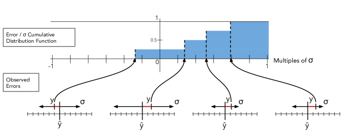
Figure 3: Visualization of the assumption made about the relationship between the underlying uncertainty distribution function and the observed errors: errors, scaled by $\sigma$, can be seen as samples from this underlying distribution function.

2.2 Aleatoric and Epistemic Uncertainty

A recurring topic when discussing sources of uncertainty is the distinction between the two primary forms of uncertainty: aleatoric uncertainty corresponds to inherent uncertainty in the data (which cannot be eliminated by collecting more data), while epistemic uncertainty, or knowledge uncertainty, corresponds to uncertainty derived from not having sufficient data in a certain region, typically manifested in the form of variance in the model parameters [Kendall and Gal, 2017]. In addition, Kendall and Gal [2017] discussed broadly the value of uncertainty estimates within computer vision, which motivates our analysis of the probabilistic object detection models in [Harakeh and Waslander, 2021].

As discussed in Laves et al. [2020], aleatoric uncertainty can be captured by models which are trained to predict uncertainties in order to maximize likelihood. On the other hand, one context in which epistemic uncertainty can be measured is in analyzing the variance of a neural network’s predictions with dropout [Laves et al., 2020]. Within our work, we include models which are trained to anticipate both kinds of uncertainty in order to demonstrate its generality.

2.3 Conformal Inference

Since 2005, there has been a growing literature on conformal predictors, a broad class of interpretable probabilistic models for both regression and classification [Vovk et al., 2005]. A conformal predictor uses as its central mechanism a nonconformity measure (in certain variations this measure is reduced to a function) which measures the similarity of one data point $(x_{i},y_{i})$ to a large pool of data, with the central motivation that an accurate prediction will tend to minimize this nonconformity. These scores are leveraged to create confidence bounds (and implied posterior distributions) proportional to the empirically ranked conformity of data points. In the context of regression specifically, Linusson et al. [2014] extended the utility of conformal inference with the introduction of negative nonconformity scores, which allowed for asymmetric posterior distributions (without any artificially asymmetric nonconformity scores).

Recently, several methods have been developed which apply specific variants of conformal inference for regression. These variants have found applications in drug discovery [Cortés-Ciriano and Bender, 2020] and biostatistics [Sun et al., 2017], where their computational efficiency has been highlighted as a benefit, as well as in image classification where they are applied to neural networks [Matiz and Barner, 2019]. However, conformal predictors in prior work do not incorporate the variance output from probabilistic models into their nonconformity measures: instead, as discussed in Shafer and Vovk [2008], methods that incorporate probabilistic models sample from predicted probabilistic distributions in order to get a more comprehensive set of predictions from which to calculate the nonconformity measure.

In inductive or split conformal prediction [Papadopoulos, 2008], a dataset separate from the training or validation dataset is used as the basis from which to evaluate the nonconformity of a point on which a prediction is being made. Jackknife methods in conformal inference build on this idea, incorporating variation due to leave-one-out sampling for the conformity measure - in particular, the ‘jackknife+‘ method [Barber et al., 2021] additionally incorporates variation due to the jackknife method in training. In CRUDE, these ideas are drawn upon and generalized.

3 CRUDE

3.1 Derivation

The CRUDE algorithm is designed for probabilistic regression problems, specifically for discriminative models that take input $x$ from space $\mathcal{X}$, and the output is a real valued $y\in\mathcal{R}$. The model, which we denote as $\mathcal{M}$, takes as input $x$, and outputs a pair of scale and non-negative shift parameters for each input $x$, i.e. $\mathcal{M}:\mathcal{X}\to\mathbb{R}\times\mathbb{R}_{+}$. We make no further assumptions about $\mathcal{M}$. Further, we assume that each observed output is noisy, and the noise $z\in\mathbb{R}$ of each example is drawn independently and identically from an unspecified error distribution $\mathcal{E}$ over the real line. The observation $y$ itself is then just a scaled and shifted version of this noise, where $\sigma$ (scaling factor) and $\mu$ (shifting magnitude) are the parameters predicted by $\mathcal{M}$.

Based on these assumptions, we posit the following data generating process:

$$x \in\mathcal{X}$$

$$\mu=\mu(x) =\mathcal{M}_{\text{shift}}(x)\in\mathbb{R}$$

$$\sigma=\sigma(x) =\mathcal{M}_{\text{scale}}(x)\in\mathbb{R}_{+}$$

$$z \sim\mathcal{E}$$

$$y =\mu+z\cdot\sigma$$

It may be useful to think of $\mathcal{E}$ as a distribution over z-scores, whose samples are scaled and shifted (depending on $x$) to result in observations $y$. Further, note that in practice the model $\mathcal{M}$ is likely trained to predict the mean and standard deviation of a normal distribution (or some other distribution over the real line), though we simply interpret those predictions as arbitrary scale and shift values per the data generation process described above, and discard any normality (or other distributional) assumptions.

The key objective of the CRUDE algorithm is to estimate $\mathcal{E}$, with $\hat{\mathcal{E}}$. This is done in a non-parametric way, simply by collecting sample z-scores from a hold-out calibration set $(X_{C},Y_{C})$, and constructing their empirical distribution:

$$Z_{C}=\left\{\frac{y-\mu(x)}{\sigma(x)}\bigm{|}(x,y)\in(X_{C},Y_{C})\right\},$$

$$\hat{\mathcal{E}}:=\text{Empirical}\left(Z_{C}\right).$$

The corresponding Cumulative Distribution Function (CDF), inverse CDF (Quantile function), and moments of $\hat{\mathcal{E}}$ are:

$$F_{\hat{\mathcal{E}}}(z)=\frac{\big{\lvert}\{z_{c}\leq z\mid z_{c}\in Z_{C}\}\big{\rvert}}{|Z_{C}|},$$

$$F_{\hat{\mathcal{E}}}^{-1}(p)=\inf\left\{z_{c}\in Z_{C}\mid F(z_{c})\geq p\right\},$$

$$\mathbb{E}\left[\hat{\mathcal{E}}\right]=\frac{1}{|Z_{C}|}\sum_{z_{c}\in Z_{C}}z_{c},$$ (1)

$$\mathbb{V}\left[\hat{\mathcal{E}}\right]=\frac{1}{|Z_{C}|}\sum_{z_{c}\in Z_{C}}\left(z_{c}-\mathbb{E}\left[\hat{\mathcal{E}}\right]\right)^{2}.$$ (2)

In turn, the predictive distribution on an unseen example $x_{*}\in\mathcal{X}$ is just the estimated $\hat{\mathcal{E}}$ scaled and shifted according to the predicted values $\mathcal{M}(x)$:

$$y\mid x_{*} \sim\mu(x_{*})+\sigma(x_{*})\cdot\hat{\mathcal{E}}$$

$$=\mathcal{M}_{\text{shift}}(x_{*})+\mathcal{M}_{\text{scale}}(x_{*})\cdot\hat{\mathcal{E}}.$$

More concretely, the predicted distribution on an unseen example $x_{*}$ has the following distribution functions and moments:

$$F_{x_{*}}(y)=F_{\hat{\mathcal{E}}}\left(\frac{y-\mu(x_{*})}{\sigma(x_{*})}\right),$$

$$F_{x_{*}}^{-1}(p)=\mu(x_{*})+\sigma(x_{*})\cdot F_{\hat{\mathcal{E}}}^{-1}(p),$$ (3)

$$\mathbb{E}[y\mid x_{*}]=\mu(x_{*})+\sigma(x_{*})\cdot\mathbb{E}\left[\hat{\mathcal{E}}\right],$$ (4)

$$\mathbb{V}[y\mid x_{*}]=\sigma^{2}(x_{*})\cdot\mathbb{V}\left[\hat{\mathcal{E}}\right].$$ (5)

Figure 3 provides a visual intuition of the empirical z-score distribution $\hat{\mathcal{E}}$.

Table 1: Performance on UCI Datasets. Different calibration methods evaluated across various datasets. The sharpest overall calibrated models for each task are underlined, and sharpness of the uncalibrated distribution is reported in italics. Lower scores are better for both calibration and sharpness. The abbreviation Kule. refers to the Kuleshov et al. [2018] method. Note that the calibration error here is measured as the RMSE of the calibration curve rather than the MSE, for easier comparison.

	Variational NN Sharpness				Dropout NN Sharpness				NGBoost Sharpness				Gaussian Process Sharpness
	None	MLE	Kule.	CRUDE	None	MLE	Kule.	CRUDE	None	MLE	Kule.	CRUDE	None	MLE	Kule.	CRUDE
fire	0.190	3.574	9.646	3.435	0.124	1.904	9.597	1.879	0.165	2.287	8.224	2.214	0.940	1.998	1.840	1.970
yacht	0.101	0.136	0.119	0.128	0.154	0.153	0.167	0.141	0.011	0.063	0.158	0.062	0.091	0.127	0.182	0.124
auto	0.174	0.528	0.819	0.511	0.122	0.396	0.773	0.382	0.103	0.536	0.986	0.512	0.140	0.411	0.707	0.398
diabetes	0.200	1.472	2.054	1.442	0.145	0.856	1.645	0.843	0.263	1.053	1.472	1.027	0.234	0.890	1.364	0.870
housing	0.138	0.483	1.172	0.467	0.146	0.412	1.110	0.398	0.090	0.501	1.329	0.486	0.256	0.535	0.912	0.528
energy	0.124	0.140	0.165	0.138	0.122	0.263	0.347	0.260	0.036	0.059	0.070	0.059	0.062	0.084	0.116	0.083
concrete	0.170	0.410	0.712	0.407	0.196	0.446	0.818	0.436	0.187	0.363	0.623	0.355	0.220	0.510	0.831	0.505
wine	0.462	1.604	1.585	1.593	0.129	0.939	2.405	0.935	0.506	0.951	1.186	0.941	0.251	1.079	2.009	1.067
kin8nm	0.305	0.449	0.754	0.448	0.182	0.402	0.958	0.401	0.561	0.654	0.737	0.653	0.191	0.333	0.570	0.333
power	0.236	0.243	0.333	0.242	0.112	0.283	0.997	0.283	0.194	0.236	0.390	0.236	0.087	1.490	1.162	1.347
airfoil	0.352	0.512	0.686	0.509	0.170	0.718	1.445	0.705	0.304	0.414	0.526	0.411	0.212	0.547	0.958	0.539
parkinsons	0.121	0.114	0.158	0.114	0.114	0.195	0.310	0.194	0.094	0.101	0.113	0.101	0.142	0.237	0.411	0.223
	Variational NN Calibration				Dropout NN Calibration				NGBoost Calibration				Gaussian Process Calibration
	None	MLE	Kule.	CRUDE	None	MLE	Kule.	CRUDE	None	MLE	Kule.	CRUDE	None	MLE	Kule.	CRUDE
fire	0.154	0.183	0.098	0.069	0.231	0.192	0.111	0.062	0.188	0.182	0.074	0.057	0.221	0.224	0.114	0.082
yacht	0.144	0.164	0.085	0.086	0.121	0.101	0.088	0.088	0.167	0.135	0.115	0.097	0.097	0.072	0.070	0.069
auto	0.155	0.080	0.097	0.076	0.150	0.085	0.088	0.073	0.186	0.089	0.111	0.060	0.162	0.075	0.096	0.069
diabetes	0.228	0.067	0.177	0.063	0.221	0.061	0.162	0.061	0.187	0.071	0.112	0.066	0.198	0.075	0.129	0.072
housing	0.148	0.084	0.084	0.061	0.139	0.071	0.074	0.053	0.201	0.093	0.120	0.070	0.079	0.072	0.060	0.055
energy	0.069	0.083	0.050	0.050	0.086	0.075	0.056	0.051	0.070	0.068	0.054	0.054	0.064	0.053	0.055	0.055
concrete	0.094	0.069	0.055	0.046	0.133	0.062	0.070	0.053	0.092	0.064	0.055	0.052	0.110	0.056	0.055	0.041
wine	0.101	0.096	0.046	0.032	0.240	0.045	0.180	0.037	0.078	0.057	0.035	0.032	0.182	0.046	0.108	0.032
kin8nm	0.066	0.018	0.017	0.014	0.121	0.022	0.042	0.018	0.052	0.033	0.017	0.017	0.079	0.024	0.024	0.018
power	0.016	0.018	0.015	0.015	0.138	0.021	0.052	0.015	0.024	0.023	0.015	0.015	0.160	0.189	0.091	0.012
airfoil	0.059	0.046	0.037	0.036	0.158	0.061	0.090	0.033	0.059	0.039	0.039	0.039	0.105	0.064	0.056	0.041
parkinsons	0.060	0.050	0.019	0.019	0.071	0.035	0.026	0.022	0.035	0.026	0.018	0.018	0.028	0.083	0.019	0.018

3.2 Algorithm

The CRUDE algorithm assumes that there exists a model $\mathcal{M}=(\mathcal{M}_{\text{shift}},\mathcal{M}_{\text{scale}})=(\mu,\sigma)$ already trained on the training data. The algorithm treats the model $\mathcal{M}$ as a given black-box, and does not require further access to the training data. Instead, an independent hold-out calibration set $(X_{C},Y_{C})\in(\mathcal{X}\times\mathbb{R})^{L}$ of size $L\in\mathbb{N}$ is used calibrate the model. On this hold-out calibration set we first calculate the residuals between the observed labels $y$ and the predicted shift value $\mu(x)$, and inversely scale by the predicted scale $\sigma(x)$. These z-scores are sorted and the empirical distribution $\hat{\mathcal{E}}$ formed by them is considered to be our estimate of $\mathcal{E}$. With this constructed $\hat{\mathcal{E}}$ in hand, we are now able to answer probabilistic questions about the predictive distribution for any unseen example input $x_{*}$.

Data: Held-out calibration dataset $(X_{C},Y_{C})\in(\mathcal{X}\times\mathbb{R})^{L}$

Input: Test example $x_{*}$, Target quantile level $p$, and Model $\{\mu,\sigma\}:\mathcal{X}\rightarrow(\mathbb{R},\mathbb{R}_{+})$

Output: Target quantile $q$

$Z_{C}\leftarrow[\quad]$

for $(x,y)\leftarrow(X_{C},Y_{C})$ do

       $Z_{C}\leftarrow\text{SortedInsert}\left\{Z_{C},\frac{y-\mu(x)}{\sigma(x)}\right\}$

end for

$z_{p}\leftarrow Z_{C}\left[\text{int}(p\cdot L)\right]$

$q\leftarrow\mu(x_{*})+\sigma(x_{*})\cdot z_{p}$

Algorithm 1 CRUDE calibration algorithm, predicting the calibrated $p^{th}$ quantile for input $x_{*}$

In Algorithm 1 we outline the steps to make a quantile prediction at a given level $p$, using which we can construct prediction intervals. For example, to calculate a $90^{th}$ percentile prediction interval of $y$ for a given input $x_{*}$, we invoke Algorithm 1 twice: once with $p=0.05$ and again with $p=0.95$ to obtain the lower and upper bounds of the interval respectively. Note that the construction of the sorted $Z$ can be cached in the first invocation and re-used in future queries. This results in a preprocessing run-time complexity of $O(L\log L)$ for the first time, and $O(1)$ time for all future quantile queries.

Similarly, querying the moments of the predictive distribution involves a one-time preprocessing time complexity of order $O(L)$ (to calculate Equation 1 or Equation 2), followed by a $O(1)$ time complexity for all future queries (Equation 4 or Equation 5).

In this time complexity analysis we only focus on the steps required by CRUDE, and ignore the time taken by the black-box model in computing $\mu(x_{*})$ and $\sigma(x_{*})$.

3.3 Relationship to the Conformal Framework

In addition to the posited data generative process in Sec 3.1, the CRUDE algorithm can also be understood as a variant of the Inductive Conformal Prediction (ICP) framework [Linusson et al., 2014].

A conformal predictor utilizes nonconformity measure

$$A:B\times(x,y)\rightarrow\mathbb{R}$$ (6)

where $B$ represents a bag of exchangeable examples, and $(x,y)$ is a new example whose non-conformance is being measured w.r.t $B$. In our case, $B$ the hold-out calibration dataset of size $L$:

$$B=(X_{C},Y_{C})\in(\mathcal{X}\times\mathbb{R})^{L}.$$

Conventional nonconformity measures have non-negative outputs, and such measures are typically utilized for generating two sided confidence bounds, for some confidence level $p$ in the output space. In the case of ICP, such confidence bounds correspond to prediction intervals over $y$ for a given input $x_{*}$. The calibration set $B$ is used to determine an appropriate $z_{p}$ corresponding to the desired confidence bound $p$ (e.g. $p=90\%$), such that $z_{p}$ best satisfies the condition

$$\cfrac{\big{\lvert}\{(x,y)\in B\mid A(B,(x,y))<z_{p}\}\big{\rvert}}{|B|}\approx p.$$ (7)

Then, the prediction interval $y^{[p]}|x_{*}$ over $y$ for given input $x_{*}$, and desired confidence level $p$ is:

$$y^{[p]}|x_{*}=\{y\in\mathbb{R}\mid A(B,(x_{*},y))\leq z_{p}\},$$ (8)

where $z_{p}$ is according from Equation 7.

Traditionally nonconformity measures $A$ are non-negative, where the above formulation of generating predictive internals necessarily produces symmetric bounds. Linusson et al. [2014]’s extension of this method allows for one sided bounding (and thus, a naturally asymmetric CDF) in a regression context by utilizing a nonconformity score that allows for negative values, with a value of $0$ as the maximum possible conformity. This in turn allows the specification of desired independent upper and lower bounds for prediction, $p_{l}$ and $p_{u}$ (eg. $p_{l}=5\%,p_{u}=95\%$ for an overall confidence bound of 90%). This in turn results in corresponding $z_{l}$ and $z_{u}$ as calculated from Equation 7, which are then used to generate the desired prediction interval, denoted $y^{[l,u]}|x_{*}$:

$$y^{[l,u]}|x_{*}=\{y\in\mathbb{R}\mid z_{l}\leq A(B,(x_{*},y))\leq z_{u}\}.$$ (9)

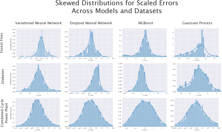
Figure 4: Visualization of the distribution of the scaled errors for each model on the Fores Fires dataset, the Diabetes dataset, and the Combined Cycle Power Plant dataset [Cortez and Morais, 2007, Kahn et al., 1993, Tüfekci, 2014]; each distribution has a skew or kurtosis.

To see the connection to CRUDE, consider a given probabilistic model $\mathcal{M}=(\mu,\sigma)$, and a nonconformity score defined as:

$$A_{\mathcal{M}}\left(B,(x,y)\right)=\cfrac{y-\mu(x)}{\sigma(x)}$$ (10)

Next, note that Equation 7 can be rewritten, given a sufficiently large calibration data $B$ of size $L$, as

$$z_{p} \approx\text{percentile}\left(\left[A_{\mathcal{M}}(B,(x,y))\mid(x,y)\in B\right],p\right)$$

$$=\text{percentile}\left(\left\{\cfrac{y-\mu(x)}{\sigma(x)}\mid(x,y)\in B\right\},p\right)$$

$$=\text{Sorted}\left\{\cfrac{y-\mu(x)}{\sigma(x)}\mid(x,y)\in B\right\}\left[\text{int}(p\cdot L)\right]$$

Note that $z_{p}$ here corresponds directly to $z_{p}$ in Algorithm 1. Now consider the prediction interval generated by CRUDE for an equivalent $p_{l}$ and $p_{u}$ as above. From Algorithm 1 we can see that:

$$y^{[l,u]}|x_{*} =\{y\in\mathbb{R}\mid\text{Algo1}(p_{l})\leq y\leq\text{Algo1}(p_{u})\}$$

$$=\{y\in\mathbb{R}\mid\mu(x_{*})+\sigma(x_{*})\cdot z_{l}\leq y$$

$$\quad\quad\quad\quad\quad\quad\leq\mu(x_{*})+\sigma(x_{*})\cdot z_{u}\}$$

$$=\left\{y\in\mathbb{R}\mid z_{l}\leq\left(\cfrac{y-\mu(x_{*})}{\sigma(x_{*})}\right)\leq z_{u}\right\}$$

$$=\left\{y\in\mathbb{R}\mid z_{l}\leq A_{\mathcal{M}}(B,(x_{*},y)\leq z_{u}\right\}$$

$$=\text{Equation}~{}\ref{eq:twosided}.$$

4 Evaluating Calibration and Sharpness

Calibration. Because we can associate each error with a likelihood in a regression prediction with uncertainty, we can evaluate the relationship between the expected and observed confidence levels. That is, for a calibrated model, the errors it predicts will be in the $30^{th}$ percentile of its distribution, should be above the observed errors 30% of the time. This is the probability integral transform (PIT) value and well-calibrated models have a uniform distribution over the percentiles associated with errors [Gneiting et al., 2007].

Ideally, each expected confidence percentile should match the fraction of values observed below the predictions of that percentile. To measure calibration, we use a variant of the Kuleshov et al. metric, measuring the RMSE between the expected confidence levels and the observed confidence levels. We use the RMSE rather than the MSE in order to more directly reflect the percent error, but the model rankings from the two approaches are unchanged. Let the test set against which we are measuring calibration be denoted $D_{T}\in(\mathcal{X}\times\mathbb{R})^{N}$ of size $N$. We initialize values of $p$ in the range $[0,1]$ with step size of $1/S$ where $S\in\mathbb{N}$ (with $S=100$ in our experiments), and for each $p_{j}$ find empirical frequency $\hat{p}_{j}$:

$$\hat{p}_{j}=\frac{1}{|D_{T}|}\sum_{(x,y)\in D_{T}}\mathbf{1}\left\{y<F_{x}^{-1}(p_{j})\right\},$$ (11)

where $F_{x}^{-1}$ is the predictive quantile function corresponding to the calibration method being evaluated. In case of CRUDE, the predictive quantile function is defined in Equation 3.

The overall calibration score across all the $S$ comparison points is then:

$$\text{cal}(\hat{p},p)=\sqrt{\frac{1}{S}\sum_{j=0}^{S}(\hat{p}_{j}-p_{j})^{2}}.$$ (12)

Sharpness. Calibration does not tell us the full story: a calibration method’s efficacy on a dataset is also based on the resulting sharpness. In order to evaluate sharpness, we can use the mean of the calibrated predicted variance on the validation set [Gneiting et al., 2007], and we take the square root of this value to match the error’s dimensionality. Note that a lower score implies higher sharpness.

5 Experiments

5.1 UCI Dataset Experiments

We evaluate each calibration method on multiple probabilistic predictive models which have shown good performance on numerous tasks, including two flavors of Bayesian neural networks, Gaussian processes, and Natural Gradient Boosting [Duan et al., 2020]. Specifically, the two neural network approaches that we consider include one using Monte Carlo dropout as described in Gal and Ghahramani [2015] as well as one which separately predicts a mean and variance [Papadopoulos et al., 2001], both with hyperparameters similar to those described in Gal and Ghahramani [2015]. Further detail about the training of these models and their architectures is provided in Appendix A.

We compare no calibration, a Gaussian maximum likelihood estimate (including shift) based on Levi et al. [2019], the Kuleshov et al. [2018] method, and CRUDE. We consider 12 datasets, mostly from the public Machine Learning Repository from the University of California, Irvine. We chose these datasets to include a variety of applications and technical features, including input dimensionality and dataset size, as well as the downstream utility of calibrated uncertainties for these predictions. We include more detail about the UCI datasets in Appendix B.

Evaluation

For each model on each dataset, we run 20 trials with the dataset shuffled and split repeatedly, with a $(0.5,0.4,0.1)$ split between training, calibration, and validation data. For each trial, we score every calibration method for calibration and sharpness. We use the metrics discussed in Section 4 for calibration and sharpness. Note that we do not use the calibration metrics proposed in Levi et al. [2019], Laves et al. [2020], as they do not consider the uncertainty distribution associated with a given uncertainty estimate, instead using mean absolute error as a metric. Moreover, as highlighted in the appendix of Laves et al., the metric implicitly corresponds to log-likelihood of the observations under a Laplacian prior, which does not match the prior that most uncertainty models are trained under.

Table 2: Bounding Box Results. Different calibration methods evaluated across various pretrained models from Harakeh and Waslander. Note again that the calibration error here is measured as the RMSE of the calibration curve rather than the MSE, for easier comparison. In addition, the calibration of the pre-trained models varies slightly from what was originally published in Harakeh and Waslander [2021]; this is due to an error in evaluation in the code base for the original paper, which has since been corrected.

		Sharpness
Detector	Loss	None	Gauss.	Kule.	CRUDE
DETR	DMM	0.004	0.113	0.265	0.110
	ES	0.014	0.132	0.203	0.130
	NLL	0.075	0.084	0.066	0.081
RetinaNet	DMM	0.011	0.125	0.241	0.109
	ES	0.016	0.109	0.198	0.097
	NLL	0.049	0.108	0.096	0.096
FasterRCNN	DMM	0.008	0.090	0.217	0.083
	ES	0.013	0.088	0.171	0.081
	NLL	0.016	0.090	0.169	0.085
		Calibration
DETR	DMM	0.136	0.172	0.074	0.011
	ES	0.111	0.161	0.040	0.011
	NLL	0.164	0.159	0.012	0.012
RetinaNet	DMM	0.184	0.113	0.091	0.012
	ES	0.147	0.112	0.058	0.012
	NLL	0.082	0.109	0.016	0.012
FasterRCNN	DMM	0.147	0.129	0.065	0.012
	ES	0.105	0.127	0.043	0.011
	NLL	0.101	0.128	0.036	0.013

5.2 Calibrated Object Detection

Following recent work on the benefits of regression uncertainty in deep object detection, we demonstrate that CRUDE can substantially improve the calibration of predictions in state-of-the-art probabilistic object detection models [Harakeh and Waslander, 2021]. While probabilistic estimates carry some inherent benefits, discussed in Kendall and Gal [2017], Harakeh and Waslander [2021] presented a probabilistic extension of a deterministic computer vision model which outperformed its corresponding deterministic model on mean Average Precision (mAP), a non-probabilistic object detection metric.

However, as with many probabilistic models, the best-performing model from the Harakeh and Waslander [2021] work, in terms of mAP, was poorly calibrated, with a RMSE of 11.1% between the ideal calibration curve and the measured calibration curve, shown in Figure 5. We note that one of the benefits of a post-hoc calibration method is the ability to apply it to pre-trained models. Specifically, we calibrate all nine of Harakeh and Waslander [2021]’s pretrained models for a bounding box regression task on the COCO [Lin et al., 2014] data, using each combination of three detectors and three loss functions.

While Harakeh and Waslander [2021] fit a Gaussian posterior to the data, we simply use the predicted mean and variance out of context to re-estimate a complete posterior using CRUDE. We split a non-repeating sample of 5,000 predicted bounding boxes from the validation set in half, and use one half for calibration and the other half to evaluate the calibration RMSE. Once again, we compare to a Gaussian MLE and the Kuleshov et al. [2018] method.

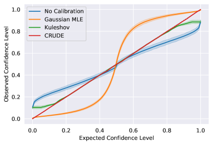
Figure 5: The calibration curves for the DETR model with an energy-based loss on the COCO [Lin et al., 2014] dataset, which was the best-performing model in Harakeh and Waslander [2021] in terms of mAP on both the COCO [Lin et al., 2014] and OpenImages [Kuznetsova et al., 2020] datasets.

6 Discussion

As highlighted in Table 1, we find that on the decisive majority of UCI dataset [Dua and Graff, 2017] tasks and models, our calibration method outperforms the alternative methods in both calibration and sharpness. There is no machine learning model that is consistently the sharpest across all datasets when calibrated, though the dropout neural network and NGBoost are disproportionately represented among the sharpest solutions.

In general, we can delineate the primary theoretical sources of error for CRUDE: the assumption that the error distributions are identical may be wrong, the assumption that the error distributions are independent may be wrong, and there may not be enough data to accurately estimate $\hat{\mathcal{D}}$. In addition, the Gaussian maximum likelihood estimation technique may outperform CRUDE if the errors are truly perfectly Gaussian, though our results indicate that in practice this is rarely the case.

We notice that the Kuleshov et al. method has the greatest likelihood of matching CRUDE on the NGBoost model in terms of calibration on larger datasets, but this tendency is not replicated for the other models. However, in almost all cases where the Kuleshov et al. method results in equal calibration, there is a substantial sacrifice of sharpness. As highlighted by Levi et al., Kuleshov et al. will be able to calibrate any distribution with enough data (excluding a very overconfident model), but it will often do so at the expense of sharpness. This is visualized by Figure 1, which shows that Kuleshov is well-calibrated, but rarely sharp, while the Gaussian MLE is often sharp, but usually more-poorly calibrated. Figure 4 shows an example scaled-error distribution on several datasets, indicating that the skew and kurtosis of the underlying error distributions may help to explain much of the improvement [Tüfekci, 2014].

On the computer vision task, as highlighted in Table 2 as well as in Figure 5, CRUDE is consistently the best-calibrated approach, and the sharpest calibrated approach on all but one model. On the best-performing model in terms of mAP, the DETR model with an energy-based loss, the calibration RMSE is reduced by 90% relative to the uncalibrated model, and 72% relative to Kuleshov [Kuleshov et al., 2018].

7 Conclusion and Future Directions

CRUDE offers substantial improvements over existing regression calibration techniques, especially for datasets where the error distribution has a nonstandard shape. However, there are many meaningful avenues left to explore. For most datasets, the assumption of a fixed uncertainty distribution, whether Gaussian or empirical, is incorrect to varying degrees. There are many ways to extend CRUDE to account for uncertainty distributions varying with respect to inputs, such as by calculating the percent-point function using only a given input’s nearest neighbors.

Similarly, treating output dimensions as independent is inadequate for many models, especially those producing a full covariance matrix as their uncertainty estimate. While this may be solvable with the inverse of pseudo-inverse of the predicted covariance matrix in place of dividing by the uncertainty in each dimension, the question of selecting a percentile over a higher-dimensional list of vectors is non-trivial. The successful incorporation of distinct epistemic and aleatoric uncertainty measurements in the calibrated distribution would be an exciting extension of CRUDE. Additionally, it may be possible to leverage the richer distributional information provided by Monte Carlo dropout. Ultimately, CRUDE opens the door to many improved regression calibration methods.

Appendix

Appendix A Model Training Information

The Gaussian processes are optimized using GPytorch with an RBF kernel and learning rate of $0.01$ [Gardner et al., 2018]. The neural networks we evaluate use three hidden layers with 1024 units each, learning rate $0.0001$, and weight decay$=0.01$. The neural networks are trained with the Adam optimizer [Kingma and Ba, 2014], with $p=0.2$ if using dropout.

Appendix B UCI Dataset Information

We analyze the Forest Fires, Yacht Hydrodynamics, Auto MPG, Diabetes, Boston Housing, Energy Efficiency, Concrete Compressive, Wine Quality, Combined Cycle Power Plant, Airfoil Self-Noise, kin8nm (not UCI), and Parkinsons Telemonitoring datasets [Cortez and Morais, 2007, Ortigosa et al., 2007, Rossi and Ahmed, 2015, Kahn et al., 1993, Harrison Jr and Rubinfeld, 1978, Tsanas and Xifara, 2012, Yeh, 1998, Cortez et al., 2009, Tüfekci, 2014, Brooks et al., 1989, Ghahramani, 1996, Tsanas et al., 2009]. The inputs range from 4 dimensional in the Power Efficiency dataset to 21 dimensional in the Parkinson’s dataset, with a median 8 dimensions. The sample count ranges from 308 examples in the Yacht Hydrodynamics dataset to 9568 examples in the Combined Cycle Power Plant dataset, with a median 899 examples.

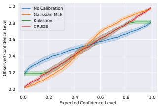
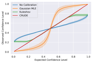
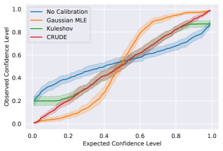
Figure 6: Various combinations of models and datasets where CRUDE performed well. In order, they are the variational neural net on the Boston Housing dataset, dropout neural net on the Parkinson’s Telemonitoring dataset, Gaussian process on the Combined Cycle Power Plant datasetm and NGBoost on the Yacht Hydrodynamics dataset.

References

- Barber et al. [2021] R. F. Barber, E. J. Candes, A. Ramdas, R. J. Tibshirani, et al. Predictive inference with the jackknife+. Annals of Statistics, 49(1):486–507, 2021.
- Brooks et al. [1989] T. F. Brooks, D. S. Pope, and M. A. Marcolini. Airfoil self-noise and prediction. 1989.
- Carvalho et al. [2015] A. Carvalho, S. Lefévre, G. Schildbach, J. Kong, and F. Borrelli. Automated driving: The role of forecasts and uncertainty—a control perspective. European Journal of Control, 24:14–32, 2015.
- Cortés-Ciriano and Bender [2020] I. Cortés-Ciriano and A. Bender. Concepts and applications of conformal prediction in computational drug discovery. Artificial Intelligence in Drug Discovery, pages 63–101, 2020.
- Cortez and Morais [2007] P. Cortez and A. J. Morais. A data mining approach to predict forest fires using meteorological data. 2007.
- Cortez et al. [2009] P. Cortez, A. Cerdeira, F. Almeida, T. Matos, and J. Reis. Modeling wine preferences by data mining from physicochemical properties. Decision Support Systems, 47(4):547–553, 2009.
- Dua and Graff [2017] D. Dua and C. Graff. UCI machine learning repository, 2017. URL http://archive.ics.uci.edu/ml.
- Duan et al. [2020] T. Duan, A. Avati, D. Y. Ding, K. K. Thai, S. Basu, A. Y. Ng, and A. Schuler. Ngboost: Natural gradient boosting for probabilistic prediction. In Proceedings of the 37th International Conference on Machine Learning, ICML 2020, 13-18 July 2020, Virtual Event, volume 119 of Proceedings of Machine Learning Research, pages 2690–2700. PMLR, 2020. URL http://proceedings.mlr.press/v119/duan20a.html.
- Gal and Ghahramani [2015] Y. Gal and Z. Ghahramani. Dropout as a bayesian approximation: Representing model uncertainty in deep learning. arXiv preprint arXiv:1506.02142, 2015.
- Gardner et al. [2018] J. R. Gardner, G. Pleiss, D. Bindel, K. Q. Weinberger, and A. G. Wilson. Gpytorch: blackbox matrix-matrix gaussian process inference with gpu acceleration. In Proceedings of the 32nd International Conference on Neural Information Processing Systems, pages 7587–7597. Curran Associates Inc., 2018.
- Ghahramani [1996] Z. Ghahramani. The kin datasets, 1996.
- Gneiting et al. [2007] T. Gneiting, F. Balabdaoui, and A. E. Raftery. Probabilistic forecasts, calibration and sharpness. Journal of the Royal Statistical Society: Series B (Statistical Methodology), 69(2):243–268, 2007.
- Harakeh and Waslander [2021] A. Harakeh and S. L. Waslander. Estimating and evaluating regression predictive uncertainty in deep object detectors. arXiv preprint arXiv:2101.05036, 2021.
- Harrison Jr and Rubinfeld [1978] D. Harrison Jr and D. L. Rubinfeld. Hedonic housing prices and the demand for clean air. 1978.
- Kahn et al. [1993] M. G. Kahn, D. Huang, S. A. Bussmann, S. B. Cousins, C. A. Abrams, and J. C. Beard. Diabetes data analysis and interpretation method, Oct. 5 1993. US Patent 5,251,126.
- Kendall and Gal [2017] A. Kendall and Y. Gal. What uncertainties do we need in bayesian deep learning for computer vision? In Proceedings of the 31st International Conference on Neural Information Processing Systems, pages 5580–5590, 2017.
- Kingma and Ba [2014] D. P. Kingma and J. Ba. Adam: A method for stochastic optimization. arXiv preprint arXiv:1412.6980, 2014.
- Kourou et al. [2015] K. Kourou, T. P. Exarchos, K. P. Exarchos, M. V. Karamouzis, and D. I. Fotiadis. Machine learning applications in cancer prognosis and prediction. Computational and structural biotechnology journal, 13:8–17, 2015.
- Kuleshov et al. [2018] V. Kuleshov, N. Fenner, and S. Ermon. Accurate uncertainties for deep learning using calibrated regression. In International Conference on Machine Learning, pages 2796–2804, 2018.
- Kumar et al. [2019] A. Kumar, P. Liang, and T. Ma. Verified uncertainty calibration. arXiv preprint arXiv:1909.10155, 2019.
- Kuznetsova et al. [2020] A. Kuznetsova, H. Rom, N. Alldrin, J. Uijlings, I. Krasin, J. Pont-Tuset, S. Kamali, S. Popov, M. Malloci, A. Kolesnikov, et al. The open images dataset v4. International Journal of Computer Vision, pages 1–26, 2020.
- Laves et al. [2020] M.-H. Laves, S. Ihler, J. F. Fast, L. A. Kahrs, and T. Ortmaier. Well-calibrated regression uncertainty in medical imaging with deep learning. In Medical Imaging with Deep Learning, 2020. URL https://openreview.net/forum?id=AWfzfd-1G2.
- Leibig et al. [2017] C. Leibig, V. Allken, M. S. Ayhan, P. Berens, and S. Wahl. Leveraging uncertainty information from deep neural networks for disease detection. Scientific reports, 7(1):1–14, 2017.
- Levi et al. [2019] D. Levi, L. Gispan, N. Giladi, and E. Fetaya. Evaluating and calibrating uncertainty prediction in regression tasks. arXiv preprint arXiv:1905.11659, 2019.
- Lin et al. [2014] T.-Y. Lin, M. Maire, S. Belongie, J. Hays, P. Perona, D. Ramanan, P. Dollár, and C. L. Zitnick. Microsoft coco: Common objects in context. In European conference on computer vision, pages 740–755. Springer, 2014.
- Linusson et al. [2014] H. Linusson, U. Johansson, and T. Löfström. Signed-error conformal regression. In Pacific-Asia Conference on Knowledge Discovery and Data Mining, pages 224–236. Springer, 2014.
- Maddox et al. [2019] W. J. Maddox, P. Izmailov, T. Garipov, D. P. Vetrov, and A. G. Wilson. A simple baseline for bayesian uncertainty in deep learning. Advances in Neural Information Processing Systems, 32:13153–13164, 2019.
- Matiz and Barner [2019] S. Matiz and K. E. Barner. Inductive conformal predictor for convolutional neural networks: Applications to active learning for image classification. Pattern Recognition, 90:172–182, 2019.
- Murata et al. [2018] A. Murata, H. Ohtake, and T. Oozeki. Modeling of uncertainty of solar irradiance forecasts on numerical weather predictions with the estimation of multiple confidence intervals. Renewable energy, 117:193–201, 2018.
- Nixon et al. [2019] J. Nixon, M. W. Dusenberry, L. Zhang, G. Jerfel, and D. Tran. Measuring calibration in deep learning. In CVPR Workshops, volume 2, 2019.
- Ortigosa et al. [2007] I. Ortigosa, R. Lopez, and J. Garcia. A neural networks approach to residuary resistance of sailing yachts prediction. In Proceedings of the international conference on marine engineering MARINE, volume 2007, page 250, 2007.
- Papadopoulos et al. [2001] G. Papadopoulos, P. J. Edwards, and A. F. Murray. Confidence estimation methods for neural networks: A practical comparison. IEEE transactions on neural networks, 12(6):1278–1287, 2001.
- Papadopoulos [2008] H. Papadopoulos. Inductive conformal prediction: Theory and application to neural networks. In Tools in artificial intelligence. Citeseer, 2008.
- Rossi and Ahmed [2015] R. A. Rossi and N. K. Ahmed. The network data repository with interactive graph analytics and visualization. In AAAI, 2015. URL http://networkrepository.com.
- Scher and Messori [2018] S. Scher and G. Messori. Predicting weather forecast uncertainty with machine learning. Quarterly Journal of the Royal Meteorological Society, 144(717):2830–2841, 2018.
- Schneider et al. [2020] P. Schneider, W. P. Walters, A. T. Plowright, N. Sieroka, J. Listgarten, R. A. Goodnow, J. Fisher, J. M. Jansen, J. S. Duca, T. S. Rush, et al. Rethinking drug design in the artificial intelligence era. Nature Reviews Drug Discovery, 19(5):353–364, 2020.
- Shafer and Vovk [2008] G. Shafer and V. Vovk. A tutorial on conformal prediction. Journal of Machine Learning Research, 9(3), 2008.
- Sun et al. [2017] J. Sun, L. Carlsson, E. Ahlberg, U. Norinder, O. Engkvist, and H. Chen. Applying mondrian cross-conformal prediction to estimate prediction confidence on large imbalanced bioactivity data sets. Journal of chemical information and modeling, 57(7):1591–1598, 2017.
- Tsanas and Xifara [2012] A. Tsanas and A. Xifara. Accurate quantitative estimation of energy performance of residential buildings using statistical machine learning tools. Energy and Buildings, 49:560–567, 2012.
- Tsanas et al. [2009] A. Tsanas, M. A. Little, P. E. McSharry, and L. O. Ramig. Accurate telemonitoring of parkinson’s disease progression by noninvasive speech tests. IEEE transactions on Biomedical Engineering, 57(4):884–893, 2009.
- Tüfekci [2014] P. Tüfekci. Prediction of full load electrical power output of a base load operated combined cycle power plant using machine learning methods. International Journal of Electrical Power & Energy Systems, 60:126–140, 2014.
- Vovk et al. [2005] V. Vovk, A. Gammerman, and G. Shafer. Conformal prediction. Algorithmic learning in a random world, pages 17–51, 2005.
- Yeh [1998] I.-C. Yeh. Modeling of strength of high-performance concrete using artificial neural networks. Cement and Concrete research, 28(12):1797–1808, 1998.
- Zhu et al. [2019] Y. Zhu, N. Zabaras, P.-S. Koutsourelakis, and P. Perdikaris. Physics-constrained deep learning for high-dimensional surrogate modeling and uncertainty quantification without labeled data. Journal of Computational Physics, 394:56–81, 2019.