Quench dynamics in disordered two-dimensional Gross-Pitaevskii Lattices

Abstract

We numerically investigate the quench expansion dynamics of an initially confined state in a two-dimensional Gross-Pitaevskii lattice in the presence of external disorder. The expansion dynamics is conveniently described in the control parameter space of the energy and norm densities. The expansion can slow down substantially if the expected final state is a non-ergodic non-Gibbs one, regardless of the disorder strength. Likewise stronger disorder delays expansion. We compare our results with recent studies for quantum many body quench experiments.

I Introduction

Quench dynamics is a common way to explore the cooling process of nonequilibrium states in Hamiltonian systems. It implicitly assumes the ability of the system to thermalize and equilibrate. The quench dynamics is particularly important when investigating localization-delocalization phenomena and the related presence or absence of thermalization Polkovnikov et al. (2011). Quench dynamics is therefore also widely used for measuring the different time scales involved in a thermalization process.

Recent experiments with interacting ultracold bosonic atomic gases loaded into two-dimensional disordered optical potentials used the quench dynamics to explore the signatures of the many-body localization-delocalization transition Choi et al. (2016). The atomic gas was confined and prepared in a thermal state and then allowed to expand into a previously empty part of the random potential. Localization-delocalization transitions were observed upon varying the disorder strength and the atom-atom interaction strength. Subsequent computational studies with quantum many-body platforms using Gutzwiller mean field methods Yan et al. (2017) and tensor network methods Urbanek and Soldán (2018) pointed to a number of open questions such as the impact of the system size and measurement times.

The dynamics of ultracold bosonic atoms in a deep optical lattice can be modeled with a Bose-Hubbard Hamiltonian (BH). For sufficiently large occupation numbers its classical counterpart—the discrete Gross-Pitaevskii (DGP) Hamiltonian—serves as a reasonable approximation Dutta et al. (2015). The experimental studies of Choi et al. were performed deep in the quantum regime with at most double occupancy per lattice site (see supplement of Ref. Choi et al. (2016)). Despite that discrepancy, the merit in the DGP approach is that large systems can be evolved up to large times using standard computational approaches and average computational resources. The DGP Hamiltonian is also known as the discrete nonlinear Schrödinger (DNLS) Hamiltonian Kevrekidis (2009) and serves as a platform to study various properties of nonlinear wave dynamics.

Many body localized phases are expected to be non-ergodic and non-thermalizing Abanin et al. (2019), at variance to their delocalized (metallic) counterparts. Many body localized phases are as well expected to be unique for quantum many body dynamics, at variance to classical wave dynamics. Therefore the DGP model can be expected not to possess a many-body localization-delocalization transition. However, the classical DGP model, as well as its quantum BH counterpart, exhibit a non-Gibbs phase, which is characterized by at least partial nonergodic properties and absence of full thermalization Mithun et al. (2018); Cherny et al. (2019). An intriguing question is therefore whether these non-Gibbs phases have an impact on the outcome of the quench dynamics.

The article is organized as the following. In section II we introduce the DGP model and its statistical description. In section III we present our results on the quench dynamics of the DGP. In the section IV we compare our numerical results with the experimental results reported in Choi et al. (2016). The section V concludes and discusses the results.

II The Model

We consider the following two-dimensional DGP Hamiltonian in dimensionless unit

$$\mathcal{H}= \sum_{n}\sum_{m}\frac{U}{2}|\psi_{m,n}(t)|^{4}+V_{m,n}|\psi_{m,n}(t)|^{2}$$

$$-J\Big{[}\psi^{*}_{m,n}(t)\psi_{m+1,n}(t)+\psi_{m,n}(t)\psi^{*}_{m+1,n}(t)$$

$$+\psi^{*}_{m,n}(t)\psi_{m,n+1}(t)+\psi_{m,n}(t)\psi^{*}_{m,n+1}(t)\Big{]},$$ (1)

where $J$ is the hopping strength, ($\psi_{m,n}(t)$, $\psi^{\ast}_{m,n}(t)$) represent the conjugated variables and the indices ($m$, $n$) represent the lattice sites in a square lattice. Here $U$ is the nonlinearity parameter and $V_{m,n}$ represents the uncorrelated onsite disorder potential of the form

$$V_{m,n} =\epsilon_{m,n}~{} \text{for}~{}1\leq m\leq L,1\leq n\leq L;$$

$$=\infty~{} \text{otherwise}.$$ (2)

The uncorrelated onsite energies $\epsilon_{m,n}$ are taken from a uniform distribution with the range $\in$ $\left[-\frac{W}{2},\frac{W}{2}\right]$. This potential enforces fixed boundary conditions $\psi_{m,n}=0$ outside the boundary ($m=1,L$; $n=1,L$) at all times $t$.

The Hamiltonian, Eq. (II) gives the following equations of motion

$$i\frac{\partial}{\partial t}\psi_{m,n}(t)=U|\psi_{m,n}(t)|^{2}\psi_{m,n}(t)+V_{m,n}\psi_{m,n}(t)\hskip 28.45274pt$$

$$-J\Big{[}\psi_{m+1,n}(t)+\psi_{m-1,n}(t)+\psi_{m,n+1}(t)+\psi_{m,n-1}(t)\Big{]}.$$ (3)

Eq. (3) possesses two conserved quantities, the total norm $\mathcal{N}$ = $\sum_{m,n}|\psi_{m,n}|^{2}$ and the total energy $\mathcal{H}$. Corresponding to the two conserved quantities, we define the norm density $a=\frac{\mathcal{N}}{L^{2}}$ and the energy density $h=\frac{\mathcal{H}}{L^{2}}$. In the absence of nonlinearity $U=0$ and disorder the solutions are plane waves $\exp[i(k_{m}m+k_{n}n-\omega_{k}t)]$ with $\omega_{k}=-2J(\cos k_{m}+\cos k_{n})$. It follows that the linear system (even with disorder) has a spectrum of eigenfrequencies (or eigenenergies) whose width amounts to $\Delta\omega=8J+W$.

If the microcanonical dynamics generated by (3) is ergodic, then infinite time averages of observables are equal to their phase space averages, and the statistical properties of the system can be described using the Gibbs grand-canonical partition function

$$Z=\int e^{-\beta(\mathcal{H}+\mu\mathcal{N})}\prod_{m=1}^{L}\prod_{n=1}^{L}d\psi_{m,n}d\psi_{m,n}^{\ast}.$$ (4)

Here $\beta$ is the inverse temperature and $\mu$ is chemical potential. It follows that the density pair $\{a,h\}$ can be mapped onto a pair of Gibbs parameters $\{\mu,\beta\}$ and vice versa. In the following we will use scaled densities $x=Ua$ and $y=Uh$. Since the seminal publications Rasmussen et al. (2000); Johansson and Rasmussen (2004) it is known, that the one-dimensional ordered discrete nonlinear Schrödinger lattice has a groundstate line $y_{0}(x)$ on which the temperature vanishes $\beta^{-1}=0$. At the same time there is a second line $y_{\infty}(x)=x^{2}>y_{0}(x)$ on which the temperature diverges $\beta=0$. All microcanonical states $y(x)>y_{\infty}(x)$ can not be described by a Gibbs distribution with a positive temperature, and negative temperature assumptions lead to a divergence of the partition function (technically this happens only on infinite systems; we will assume here that our considered system sizes are large enough for this statement to apply). Recently these results were generalized to Gross-Pitaevskii lattices with any lattice dimension and disorder, and even to corresponding quantum many-body interacting Bose-Hubbard lattices Cherny et al. (2019). While the zero-temperature line $y_{0}(x)$ renormalizes in the presence of a disorder potential, the infinite temperature line $y_{\infty}(x)=x^{2}$ is invariant under the addition of disorder.

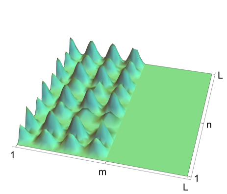
Figure 1: Schematic distribution of the initial wave function norm $|\psi_{m,n}|^{2}$ profile on a square lattice of size $L\times L$ with fixed boundary conditions. Inside the square lattice the initial wavefunction is strictly zero for $m>L/2$.

We use a symplectic scheme Yoshida (1990); McLachlan (1995); Laskar and Robutel (2001) to numerically integrate Eq. (3). The details of the symplectic integration method $\mathcal{SBAB}_{2}$ can be found in Refs. Skokos et al. (2009, 2014); Danieli et al. (2019). We consider time steps $\Delta t=0.005$ to keep the relative error in energy $\Delta H=(H(t)-H(0))/H(0)$ and norm $\Delta\mathcal{N}=(N(t)-N(0))/N(0)$ smaller than $10^{-3}$.

III Quench dynamics

We consider a square lattice of size $L\times L$ with $L=16$. We set the total norm $\mathcal{N}=125$ in loose analogy to the experiments Choi et al. (2016) which trapped 125 atoms. Thus roughly one unit of norm in our numerical experiments corresponds to one atom. We prepare an initial state of plane waves $\psi_{m,n}(t=0)$ = $\sqrt{a_{0}}e^{i\phi_{m,n}(t=0)}$ if $m$ $\in$ $\left\{1,2,3,\ldots,\big{\lfloor}\frac{L}{2}\big{\rfloor}\right\}$ occupying one (left) half of the system $\mathcal{L}$, i.e. $\psi_{m,n}=0$ for $m$ $\in$ $\left\{\big{\lfloor}\frac{L}{2}\big{\rfloor}+1,\big{\lfloor}\frac{L}{2}\big{\rfloor}+2,\ldots,L\right\}$ in the right half of the system $\mathcal{R}$. Fig. 1 shows the schematic representation of the initial state. The initial norm density in the excited half $\mathcal{L}$ of the system is $a_{0}=\frac{125}{L^{2}/2}\approx 0.98$ (before the quench). If the excitation spreads over the entire system, the expected final norm density in the entire system (after the quench) becomes $a=\frac{125}{L^{2}}\approx 0.49$.

We follow the evolution of the local norm density $|\psi_{m,n}|^{2}$. In addition to the real space imaging of $|\psi_{m,n}|^{2}$ at the final time, we measure the time evolution of the left-right norm imbalance ratio:

$$I(t)=\frac{\sum_{(m,n)\in\mathcal{L}}|\psi_{m,n}(t)|^{2}-\sum_{(m,n)\in\mathcal{R}}|\psi_{m,n}(t)|^{2}}{\sum_{(m,n)\in\mathcal{L}}|\psi_{m,n}(t)|^{2}+\sum_{(m,n)\in\mathcal{R}}|\psi_{m,n}(t)|^{2}}.$$ (5)

The imbalance is bounded by $|I|\leq 1$. At $t=0$ it follows $I(0)=1$. Further, at equilibrium $\sum_{(m,n)\in\mathcal{L}}|\psi_{m,n}|^{2}=\sum_{(m,n)\in\mathcal{R}}|\psi_{m,n}|^{2}$. Hence after some equilibration time $t_{\text{eq}}$ the norm imbalance practically vanishes $I(t\geq t_{\text{eq}})$ $\approx$ 0.

In the absence of nonlinearity, $U=0$, the Eq. (3) is integrable and analytically solvable. For the linear ordered case $U=0$, $W=0$ a set of plane waves appear as the eigenfunctions. In this case it follows that the imbalance ratio will show large amplitude oscillations with time, without any tendency to thermalize and diminishing of the oscillation amplitudes. In presence of disorder, $W\neq 0$ the system shows Anderson localization Anderson (1958). The initial state will not propagate into the entire system, and the imbalance $I$ will saturate at some nonzero value depending on $W$. The presence of nonlinearity destroys integrability. This will usually lead to a restoring of ergodicity, and thermalization. Consequently the imbalance is expected to saturate at value zero. At variance to classical field equations, quantum many body interacting systems can show many-body localization phases which withstand the above scenario Abanin et al. (2019), so that the imbalance is expected to saturate at a nonzero value. This precise prediction was tested in the experiments on cold atoms Choi et al. (2016). However, the DGP system while being classical also possesses nonergodic phases as discussed above. In order to study the impact of the nonergodic DGP phase on the quench dynamics, we will study the quench dynamics in the regime of weak nonlinear interactions $x\ll 1$, strong nonlinear interactions $x\gg 1$, and for strong nonlinear interactions tuned close to the experimental parameters in Ref. Choi et al. (2016).

III.1 Quench dynamics in the Gibbs regime

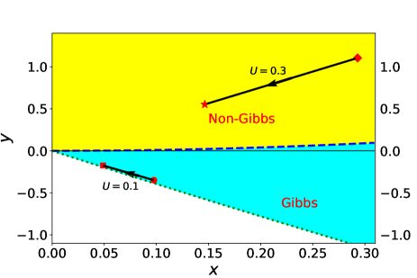
Figure 2: Small Nonlinearity $x\ll 1$: Phase diagram for the ordered case in the density parameter space $(x,y)$. The blue dashed curve is the transition line $y=x^{2}$ between the Gibbs (cyan) and non-Gibbs (yellow) regimes ($\beta=0$). The green dotted line is the ground state line for the ordered system $y=-4x+x^{2}/2$ ($\beta=\infty$). Each pair of symbols connected by lines with arrows denotes an initial state (larger norm density $x$) and the expected final state after the quench (smaller norm density $x$). The corresponding values of $U=0.1$ and $U=0.3$ are denoted right to the pair lines.

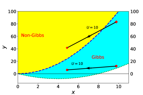
Figure 3: Large nonlinearity $x\gg 1$. Notations are as in Fig. 2.

We first consider quenches which start and end in the Gibbs regime. We use $\phi_{m,n}(t=0)=0$. This choice starts the dynamics close to the ordered system ground state line $y=-4x+x^{2}/2$ and keeps the system in the Gibbs regime after the quench, irrespective of the value of $U$.

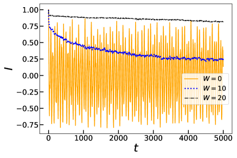
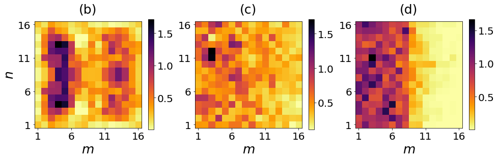
Figure 4: Quench dynamics for the $U=0.1$ path in Fig. 2. (a) Imbalance $I(t)$ for $W=0,10,20$. (b)-(d) Norm density distribution at final time $t=5000$. (b) $W=0$, (c) $W=10$, (d) $W=20$. All data for $W\neq 0$ are averaged over 20 disorder realizations.

For weak nonlinearity $U=0.1$ the quench line is shown in Fig. 2 to connect the red circle and square. The evolution outcome is shown in Fig. 4 for three different values of disorder strength $W=0,10,20$. As expected, for $W=0$ the imbalance $I(t)$ shows non-decaying large amplitude oscillations around zero. It indicates absence of thermalization of the system up to the final evolution time, as also seen from the final time density plot snapshot in Fig. 4(b). As $W$ increases, Anderson localization prevails on the time scales of the runs. The imbalance decay is slowing down and nearly saturates during the later time of evolution for $W=10,20$. The snapshots of the final time density plots in Figs. 4(c) and 4(d) confirm the above findings.

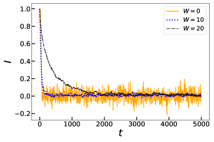
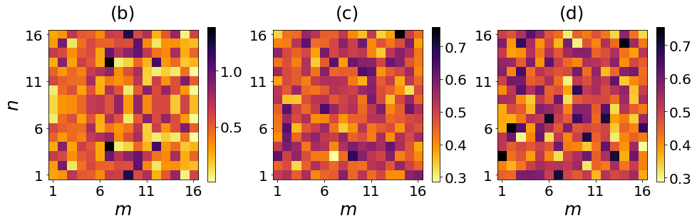
Figure 5: Quench dynamics for the $U=10$ path in Fig. 3. (a) Imbalance $I(t)$ for $W=0,10,20$. (b)-(d) Norm density distribution at final time $t=5000$. (b) $W=0$, (c) $W=10$, (d) $W=20$. All data for $W\neq 0$ are averaged over 20 disorder realizations.

For strong nonlinearity $U=10$ the quench line is shown in Fig. 3 to connect the red filled diamond and star. We observe thermalization and a decay of the imbalance to zero for all values of disorder $W=0,10,20$ in Fig. 5. The thermalized density clouds at the final simulation times are shown in Figs. 5(b, c, d).

III.2 Quench Dynamics in the Non-Gibbs regime

We consider quenches which either start in the non-Gibbs regime and therefore stay in it, or which start in the Gibbs regime, but transit into the non-Gibbs one. We initialize our system wavefunction with phases $\phi_{m,n}(t=0)=\pi(m+n)$ so that the phase difference between any two nearest lattice neighbors is $\pi$. For weak nonlinearity $U=0.3$ the quench path connects the triangle and the cross in Fig. 2. The evolution outcome is shown in Fig. 6. For $W=0$ we observe the formation of three persistent long-lived strongly localized large amplitude excitations Fig. 6(b). Each of them confines a norm of about 30, which leaves a norm of about 35 to the background (barely visible). Since two of the peaks are located in the left part and one in the right, the imbalance should take a value of about $30/125=0.24$ assuming that the background thermalizes. The dependence $I(t)$ in Fig. 6(a) nicely confirms these findings. Note that previous studies have observed and discussed the condensation of excess norm into strongly localized excitations such that the background will evolve at an infinite temperature Rasmussen et al. (2000); Johansson and Rasmussen (2004); Rumpf (2004). Increasing the strength of disorder to $W=10$ we still observe remnants of this non-Gibbs dynamics, while even stronger disorder $W=20$ reinforces Anderson localization features.

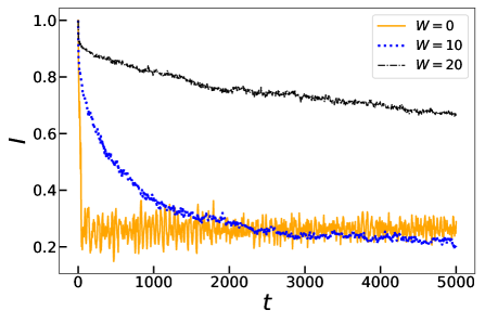
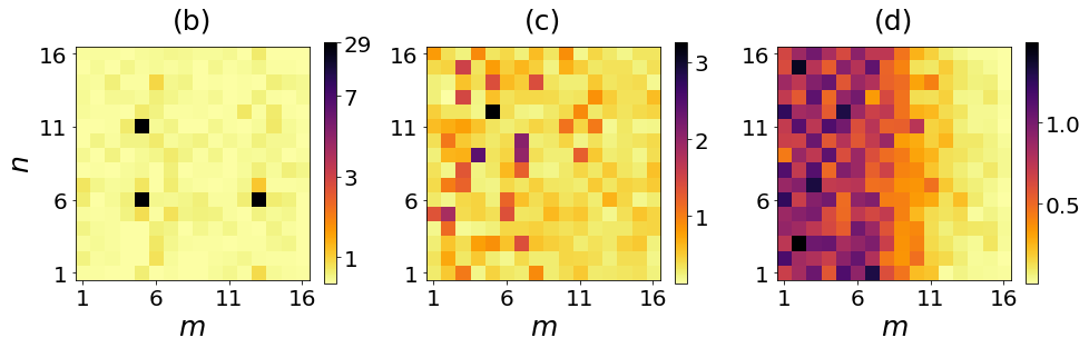
Figure 6: Quench dynamics for the $U=0.3$ path in Fig. 2. (a) Imbalance $I(t)$ for $W=0,10,20$. (b)-(d) Norm density distribution at final time $t=5000$. (b) $W=0$, (c) $W=10$, (d) $W=20$. All data for $W\neq 0$ are averaged over 20 disorder realizations.

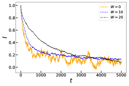
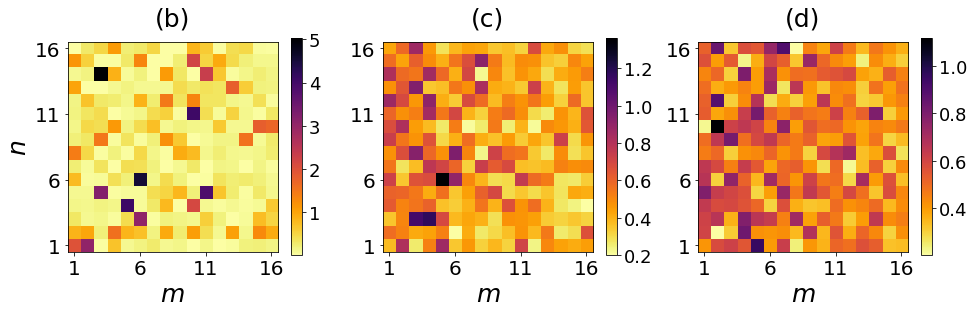
Figure 7: Quench dynamics for the $U=10$ path in Fig. 3. (a) Imbalance $I(t)$ for $W=0,10,20$. (b)-(d) Norm density distribution at final time $t=5000$. (b) $W=0$, (c) $W=10$, (d) $W=20$. All data for $W\neq 0$ are averaged over 20 disorder realizations.

For strong nonlinearity $U=10$ the quench path connects the red filled diamond (Gibbs) and star (non-Gibbs) in Fig. 3. The evolution outcome is shown in Fig. 7. For $W=0$ we again observe the formation of several (5-6) persistent long-lived strongly localized large amplitude excitations Fig. 7(b). Each of them confines a norm of about 5 so that the imbalance should take values about $0.04...0.1$ which is close to the observed dependence $I(t)$ in Fig. 7(a). Increasing the strength of disorder to $W=10$ we still observe remnants of this non-Gibbs dynamics with an additional delay in the relaxation of $I(t)$, while even stronger disorder $W=20$ reinforces Anderson localization features.

IV Revisiting experimental data

The experiments with interacting ultracold bosonic atomic gases loaded into two-dimensional disordered optical potentials discussed in the introduction result in imbalance curves shown in Fig. 8. The experimental curves show that the imbalance relaxation slows down with increasing disorder strength, and develops a nonzero asymptotic value. We note that the disorder potential in the experiment had a Gaussian distribution, with full width at half maximum $\Delta$ which corresponds to a variance $\Delta^{2}/(8\ln(2))$ Choi et al. (2016). The box disorder which we use in this work has variance $\sigma^{2}=W^{2}/12$, thus we assume $\Delta/J=\sqrt{2\ln(2)/3}W$. Mapping the experimental setup onto models of interacting bosons results in an interaction strength of $U=24.4$ Choi et al. (2016). We also note that the experimental records extend to a largest observation time of $t=300$.

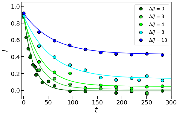
Figure 8: $I(t)$ for various disorder strength values parameterized through the full width half maximum $\Delta$ (see text for details), as observed in the experiment. Solid curves guide the eye and correspond to $I(t)=I_{0}\exp(-t/t_{s})+I_{\infty}$. We read $I_{\infty}$ off the last three experimental data points, and $t_{s}$ from the inset of Fig. 2 in Ref. Choi et al. (2016).

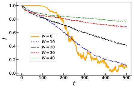
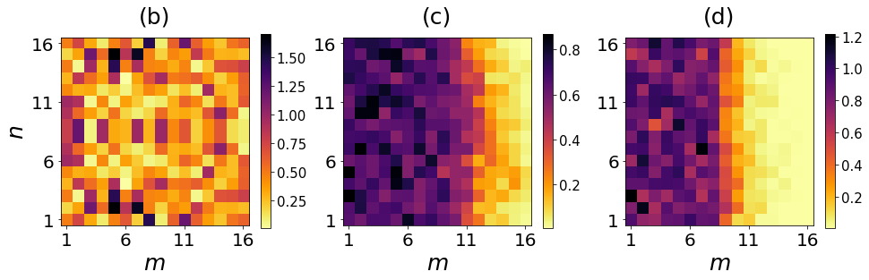
Figure 9: Gibbs quench dynamics for $U=24.4$. (a) Imbalance $I(t)$ for $W=0,10,20,30,40$. (b)-(d) Norm density distribution at final time $t=500$. (b) $W=0$, (c) $W=20$, (d) $W=40$. All data for $W\neq 0$ are averaged over 20 disorder realizations.

In order to compare the experimental results to the DGP dynamics, we use our previous setup with $U=24.4$ and launch the system in the Gibbs regime with initial conditions as in section III.1. The Gibbs regime choice follows from the experimental data which show a quick relaxation of the imbalance in the absence of disorder. Our results are shown in Fig. 9. We observe that the imbalance relaxation is actually delayed for the ordered case compared to the disordered cases. The reason is that the energy shift $U|\psi_{m,n}|^{2}$ at each excited cite amounts to $24.4$. Recall that the spectral width of the unexcited lattice part amounts to $\Delta\omega=8+W$. It follows that the excited half of the lattice at $W=0$ is tuned out of resonance (similar to self trapping) with the unexcited one. At variance, nonzero disorder removes the out-of-resonance feature of the initial state, leading to faster initial decay of the imbalance. At the same time, stronger disorder hinders full propagation of the excitation into the entire system, which results in a substantial delay of the imbalance decay at larger time, with almost freezing features at $W=40$. We conclude that the experimental data obtained in the deep quantum regime show some similarities and differences to the classical runs.

V Discussion and Conclusions

We investigated the quench expansion dynamics of an initially confined state in a two-dimensional Gross-Pitaevskii lattice in the presence of external disorder. The expansion dynamics can show qualitatively different outcomes for the imbalance evolution $I(t)$, which depend on the system path in the control parameter space of the energy and norm densities. The density space contains a non-Gibbs region. The dynamics in that region leads to strong selftrapping and focusing of potentially large (compared to the average density) norm on essentially single lattice sites. Thermalization in the non-Gibbs regime can or will be substantially delayed if not completely suppressed, leading to a freezing of the imbalance. On the other side, quenches in the Gibbs regime in general result in an imbalance decay, which however can be tremendously postponed by adding strong disorder.

We compared our results to recent experiments with interacting ultracold bosonic atomic gases loaded into two-dimensional disordered optical potentials Choi et al. (2016). Non-Gibbs dynamics is possible for quantum interacting systems as well Cherny et al. (2019). However the experimental setup reported at most double occupancy per site, which means that the optical potential setup was not capable of trapping more interacting atoms per site. Therefore, the impact of non-Gibbs phases can be excluded for the experimental setup. At the same time we find at least qualitatively similar results for the imbalance relaxation in the Gibbs regime of our system.

References

- Polkovnikov et al. (2011) A. Polkovnikov, K. Sengupta, A. Silva, and M. Vengalattore, “Colloquium: Nonequilibrium dynamics of closed interacting quantum systems,” Rev. Mod. Phys. 83, 863 (2011).
- Choi et al. (2016) J.-y. Choi, S. Hild, J. Zeiher, P. Schauß, A. Rubio-Abadal, T. Yefsah, V. Khemani, D. A. Huse, I. Bloch, and C. Gross, “Exploring the many-body localization transition in two dimensions,” Science 352, 1547 (2016).
- Yan et al. (2017) M. Yan, H.-Y. Hui, M. Rigol, and V. W. Scarola, “Equilibration dynamics of strongly interacting bosons in 2d lattices with disorder,” Phys. Rev. Lett. 119, 073002 (2017).
- Urbanek and Soldán (2018) M. Urbanek and P. Soldán, “Equilibration in two-dimensional bose systems with disorders,” The European Physical Journal D 72, 114 (2018).
- Dutta et al. (2015) O. Dutta, M. Gajda, P. Hauke, M. Lewenstein, D.-S. Lühmann, B. A. Malomed, T. Sowiński, and J. Zakrzewski, “Non-standard hubbard models in optical lattices: a review,” Reports on Progress in Physics 78, 066001 (2015).
- Kevrekidis (2009) P. G. Kevrekidis, The discrete nonlinear Schrödinger equation: mathematical analysis, numerical computations and physical perspectives, Vol. 232 (Springer Science & Business Media, 2009).
- Abanin et al. (2019) D. A. Abanin, E. Altman, I. Bloch, and M. Serbyn, “Colloquium: Many-body localization, thermalization, and entanglement,” Rev. Mod. Phys. 91, 021001 (2019).
- Mithun et al. (2018) T. Mithun, Y. Kati, C. Danieli, and S. Flach, “Weakly nonergodic dynamics in the gross-pitaevskii lattice,” Phys. Rev. Lett. 120, 184101 (2018).
- Cherny et al. (2019) A. Y. Cherny, T. Engl, and S. Flach, “Non-gibbs states on a bose-hubbard lattice,” Phys. Rev. A 99, 023603 (2019).
- Rasmussen et al. (2000) K. O. Rasmussen, T. Cretegny, P. G. Kevrekidis, and N. Grønbech-Jensen, “Statistical mechanics of a discrete nonlinear system,” Phys. Rev. Lett. 84, 3740 (2000).
- Johansson and Rasmussen (2004) M. Johansson and K. O. Rasmussen, “Statistical mechanics of general discrete nonlinear schrödinger models: Localization transition and its relevance for klein-gordon lattices,” Phys. Rev. E 70, 066610 (2004).
- Yoshida (1990) H. Yoshida, “Construction of higher order symplectic integrators,” Physics letters A 150, 262 (1990).
- McLachlan (1995) R. I. McLachlan, “Composition methods in the presence of small parameters,” BIT Numerical Mathematics 35, 258 (1995).
- Laskar and Robutel (2001) J. Laskar and P. Robutel, “High order symplectic integrators for perturbed hamiltonian systems,” Celestial Mechanics and Dynamical Astronomy 80, 39 (2001).
- Skokos et al. (2009) C. Skokos, D. Krimer, S. Komineas, and S. Flach, “Delocalization of wave packets in disordered nonlinear chains,” Physical Review E 79, 056211 (2009).
- Skokos et al. (2014) C. Skokos, D. Krimer, S. Komineas, and S. Flach, “Erratum: Delocalization of wave packets in disordered nonlinear chains phys. rev. e 79, 056211 (2009),” Physical Review E 89, 029907 (2014).
- Danieli et al. (2019) C. Danieli, B. M. Manda, M. Thudiyangal, and C. Skokos, “Computational efficiency of numerical integration methods for the tangent dynamics of many-body hamiltonian systems in one and two spatial dimensions,” Mathematics in Engineering 1, 447 (2019).
- Anderson (1958) P. W. Anderson, “Absence of diffusion in certain random lattices,” Phys. Rev. 109, 1492 (1958).
- Rumpf (2004) B. Rumpf, “Simple statistical explanation for the localization of energy in nonlinear lattices with two conserved quantities,” Phys. Rev. E 69, 016618 (2004).