On Optimal Partitioning For Sparse Matrices In Variable Block Row Format

Abstract

The Variable Block Row (VBR) format is an influential blocked sparse matrix format designed for matrices with shared sparsity structure between adjacent rows and columns. VBR groups adjacent rows and columns, storing the resulting blocks that contain nonzeros in a dense format. This reduces the memory footprint and enables optimizations such as register blocking and instruction-level parallelism. Existing approaches use heuristics to determine which rows and columns should be grouped together. We show that finding the optimal grouping of rows and columns for VBR is NP-hard under several reasonable cost models. In light of this finding, we propose a 1-dimensional variant of VBR, called 1D-VBR, which achieves better performance than VBR by only grouping rows. We describe detailed cost models for runtime and memory consumption. Then, we describe a linear time dynamic programming solution for optimally grouping the rows for 1D-VBR format. We extend our algorithm to produce a heuristic VBR partitioner which alternates between optimally partitioning rows and columns, assuming the columns or rows to be fixed, respectively. Our alternating heuristic produces VBR matrices with the smallest memory footprint of any partitioner we tested.

1 Introduction

Matrices that occur in practice are often sparse, meaning that most of their entries are zero, and it is faster to process only the nonzero entries[1, 2]. Some applications produce matrices where nonzeros occur close together. In these cases, we can reduce the complexity and storage requirements of processing and locating individual nonzeros by storing the nonzeros in dense blocks. We need only store the size and location of the block, and can employ dense performance engineering techniques like register blocking and instruction-level parallelism.

Blocked formats are most commonly used to accelerate multiplication between a sparse matrix and a dense vector (SpMV). SpMV is often used as a subroutine in iterative solvers; the same sparse matrix is multiplied hundreds of times before a solution is found. A practical use case is to block the matrix once, then offset the cost of finding the blocks and converting the matrix format with the savings obtained after multiplying the matrix many times in an iterative solver.

Dense blocks have also been used in supernodal sparse factorizations [3, 4], incomplete factorizations [1, 5] and in sparse triangular solves [6]. Originally, only rows/columns with identical sparsity patterns were merged, but the approach can be relaxed to merge rows/columns with merely similar patterns [7]. Note that for preconditioning, block methods are mathematically different and may affect the convergence rate, typically making methods more robust. Kim et. al. [8] extended the “algorithms by block” concept from dense to sparse linear algebra and showed it is useful for task parallel systems on modern architectures.

One of the first blocked formats to receive considerable study was the Variable Block Row (VBR) format, where similar adjacent rows and columns are grouped together [9, 10, 11]. VBR is described in the SPARSKIT library [12, 13], the SparseBLAS specification [14], and the OSKI Sparse Kernel Interface [15, 2], and is used internally by the MKL Paradiso solver [16]. Unlike many formats which use fixed-size blocks, the number of rows or columns that may be grouped together is allowed to vary along each dimension, producing variably sized blocks. Since blocks are produced by merging entire rows or columns, the blocks are aligned, allowing implementations to reuse elements of other arguments along the direction of alignment. In general, producing bigger blocks means that less location information is needed, but as blocks get bigger, they may cover and store more zeros explicitly in dense storage.

While the VBR format was motivated by scientific applications that produce matrices with perfect block structure (where nearby rows with identical patterns might represent different partial derivatives of the same variable or different variables of the same multiphysics mesh point), we investigate the application of these techniques to sparse matrices with imperfect block structure (where nearby rows with correlated patterns might represent neighboring mesh points or similar mathematical programming constraints).

Block partitioning algorithms sometimes reorder rows to group similar rows together [17, 5, 18]. In this work, as in the definition of VBR, we consider only contiguous partitions (splitting without reordering). While noncontiguous partitions allow for more expressive blocks, permuting a matrix or vector may be an expensive memory-intensive procedure. In some situations, the matrix may have already been reordered for numerical reasons, and the user might need to operate on the matrix without changing the row ordering. Furthermore, there are several matrices which do not need reordering to utilize similarities among adjacent rows. Our cost models apply to contiguous or noncontiguous partitions alike, and research into contiguous partitioning may inform general partitioning approaches.

Although the contiguous case may appear simpler, in Appendix A, we prove that determining optimal groupings of adjacent rows and columns for VBR format is NP-Hard under two simple cost models by reduction from the Maximum Cut problem [19, 20]. The problem is still NP-Hard even when the row and column partitions are constrained to be the same, a symmetric constraint required by some block factorizations. In light of this observation, we invent a specialization of the VBR sparse matrix format for the case where the columns are simply ungrouped, making optimal partitioning tractable. We refer to this new, simpler, format as 1D-VBR. 1D-VBR enjoys many of the same benefits as VBR, obtaining better performance at the cost of slightly more memory usage.

At the time of writing, only heuristic algorithms have been given to determine which rows or columns should be grouped together. We first propose detailed cost models which describe the number of blocks, the memory footprint, or the expected SpMV runtime of the resulting VBR or 1D-VBR format, inspired by [21, 10]. We then describe a linear time, single pass, algorithm to determine the optimal contiguous row groups under a fixed column grouping and general cost model, inspired by [22, 23, 24, 25, 26]. Our algorithm is optimal for 1D-VBR since ungrouped columns are a fixed column grouping. We can also build a VBR heuristic by alternately partitioning just the rows, then columns, then rows again, similar to [27, 28, 29]. Our algorithm runs in time $O(R\cdot(u_{\max}\cdot m+N)+n)$, where $R$ is the rank of the cost function (a small constant), $u_{\max}$ is the maximum block height (a small constant [30]), and $m$, $n$, and $N$ are the number of rows, columns, and nonzeros, respectively. Our algorithm requires only one pass directly on the sparse matrix in CSR format.

We test our optimal algorithm against existing heuristics on a test set of 20 ​ real-valued sparse matrices with interesting, imperfect, block structure (10 of which are the test set of [9]), in both 64 and 32 bit precision. Using our heuristic to reduce the VBR memory footprint resulted in the the best compression. Using our algorithm to minimize our empirical cost model of 1D-VBR SpMV runtime resulted in the best performance, achieving a median speedup of $2.22$$\times$ ​ over the reference CSR implementation. On at least half of the matrices, the overhead of partitioning and conversion to 1D-VBR format was justified within $16.9$ ​ multiplications, demonstrating the practicality of our techniques.

2 Partitioning

Let $A$ be an $m\times n$ matrix with $N$ nonzeros, where $A_{i,j}$ corresponds to the value in the $i^{\text{th}}$ row and $j^{\text{th}}$ column. We use $i{:}i^{\prime}$ to represent the integer sequence $i,i+1,...,i^{\prime}$, and describe submatrices of $A$ as $A_{i:i^{\prime},j:j^{\prime}}$. When the argument to a function is clear from context, we will omit the argument for brevity.

In practice, adjacent rows (and columns) often contain similar patterns of nonzero locations. To capitalize on this observation, we will group similar rows together, forming a row part. A $K$-partition $\Pi$ of rows of $A$ assigns each row $i$ to one of $K$ parts $\Pi_{k}$. In this work, we insist that our partitions stay contiguous, meaning that for $k<k^{\prime}$, $i\in\Pi_{k}$, $i^{\prime}\in\Pi_{k^{\prime}}$, we have $i<i^{\prime}$. We use $\Pi^{-1}$ to refer to the length $n$ vector of part assignments, so that when $i\in\Pi_{k}$, $\Pi^{-1}_{i}=k$. When $\Pi$ is contiguous, we can represent it with a vector $spl_{\Pi}$ of $K+1$ split points, so that $\Pi_{k}=spl_{\Pi,k}:spl_{\Pi,k+1}-1$. A partition is trivial if it assigns each row to a distinct part.

We may also impose an $L$-partition $\Phi$ of columns. The partitions $\Pi$ and $\Phi$ tile our matrix with $K\times L$ contiguous, non-overlapping, rectangular blocks. The block $(k,l)$ is of size $u_{k}\times w_{l}=|\Pi_{k}|\times|\Phi_{l}|$. Blocked formats store only nonzero blocks, or blocks that contain at least one nonzero of $A$. If we partition wisely, many blocks will be zero and not need to be stored.

We use $v_{i}(A,\Phi)=\{l|A[i,\Phi_{l}]\neq 0\}$ to refer to the set of column parts containing nonzeros in the $i^{th}$ row of $A$, and $\gamma_{k}(A,\Pi,\Phi)=\bigcup_{i\in\Pi_{k}}v_{i}$ to refer to the set of column parts containing nonzeros in the $k^{th}$ row part of $A$.

3 Sparse Formats

Sparse matrices are commonly stored in Compressed Sparse Row (CSR) format [1], which consists of three vectors $pos$, $idx$, and $val$. The length $m+1$ vector $pos$ stores the regions of $idx$ and $val$ corresponding to each row. The vectors $idx$ and $val$ (each of length $N$) store the sorted nonzero column locations and corresponding values, respectively. Storing $A$ in CSR format uses

(3.1) $$s_{\text{CSR}}(A)=(m+1)s_{\text{index}}+N\cdot s_{\text{index}}+N\cdot s_{\text{value}}$$

bits, where $s_{\text{index}}$ and $s_{\text{value}}$ are the sizes of the index and value types, in bits.

The Variable Block Row (VBR) format imposes a contiguous $K$-partition $\Pi$ of rows and a contiguous $L$-partition $\Phi$ of columns [12, 13, 14, 15, 2]. It is illustrated in Figure 1. It is convenient to store the length $K+1$ and $L+1$ split vectors $spl_{\Pi}$ and $spl_{\Phi}$, respectively. Instead of storing individual nonzero locations, the VBR format saves memory using the $idx$ vector to store block indices (the indices record the parts corresponding to each block). The positions of the variably-sized blocks in $val$ are not aligned with the positions of the block indices in the $idx$ array. Therefore, we use a vector $ofs$ of block locations to encode the starting index of each block row in $val$. Assume we were to store $A$ in VBR format and wanted to determine the value of the entry $A_{i,j}$. Let $k=\Pi^{-1}_{i}$ and $l=\Phi^{-1}_{j}$ (when partitions are contiguous, we can compute this with binary search on the split vectors). If we cannot find $q$ such that $A.pos[k]\leq q<A.pos[k+1]$ and $A.idx[q]=l$, then $A_{i,j}=0$ because the block $(k,l)$ is entirely zero and is not stored explicitly in VBR format. Otherwise, our block contains at least one nonzero and starts at position $p=A.ofs[k]+\sum_{l^{\prime}\in\gamma_{k}|l^{\prime}<l}u_{k}*w_{l^{\prime}}$ in the $val$ array. Because VBR stores nonzero blocks in a dense, column-major format, $A_{i,j}=A.val[p+(j-A.spl_{\Phi}[l])\cdot u_{k}+(i-A.spl_{\Pi}[k])]$.

Let $N_{\text{index}}(A,\Pi,\Phi)$ be the number of nonzero blocks induced by $\Pi$ and $\Phi$, so that

(3.2) $$N_{\text{index}}(A,\Pi,\Phi)=\sum\limits_{k=1}^{K}|\gamma_{k}|.$$

Let $N_{\text{value}}(A,\Pi,\Phi)$ be the number of entries contained in all nonzero blocks induced by $\Pi$ and $\Phi$, such that

(3.3) $$N_{\text{value}}(A,\Pi,\Phi)=\sum\limits_{k=1}^{K}\sum\limits_{l\in\gamma_{k}}u_{k}\cdot w_{l}.$$

The VBR format uses six arrays, $spl_{\Pi}$, $spl_{\Phi}$, $pos$, $ofs$, $idx$, and $val$. Storing $A$ in VBR format uses $s_{\text{VBR}}$ bits,

(3.4) $$s_{\text{VBR}}(A,\Pi,\Phi)=\\ (3(K+1)+(L+1)+N_{\text{index}})s_{\text{index}}+N_{\text{value}}s_{\text{value}}.$$

In this work, we introduce a novel specialization of VBR format where the column partition is trivial, meaning that the columns are not grouped together and we concern ourselves only with row partitioning. We call this special format 1D-VBR. An example is illustrated in Figure 1. Because $\Phi$ is trivial, we do not need to store it. Additionally, because blocks have only one column, block sizes are constant within each row part and the stride between blocks is constant within each row part, simplifying the implementation of conversion and multiplication routines. Assume we were to store $A$ in 1D-VBR format and wanted to determine the value of the entry $A_{i,j}$. Let $k=\Pi^{-1}[i]$. Notice that $\Phi^{-1}[j]=j$, since $\Phi$ is trivial. If we cannot find $q$ such that $A.pos[k]\leq q<A.pos[k+1]$ and $A.idx[q]=j$, then $A[i,j]=0$ because the block $(k,j)$ is entirely zero and is not stored explicitly in 1D-VBR format. Otherwise, our block contains at least one nonzero and starts at position $p=A.ofs[k]+(q-A.pos[k])\cdot u_{k}$ in the $val$ array. Thus, $A_{i,j}=A.val[p+(i-A.spl_{\Pi}[k])]$. The 1D-VBR format uses five arrays, $spl_{\Pi}$, $pos$, $idx$, $ofs$, and $val$. Storing $A$ in 1D-VBR format uses $s_{\text{1D-VBR}}$ bits,

(3.5) $$s_{\text{1D-VBR}}(A,\Pi)=\\ (3(K+1)+N_{\text{index}})s_{\text{index}}+N_{\text{value}}s_{\text{value}}.$$

3.1 Related Sparse Formats

Blocked sparse formats have enjoyed a long history of study. In lieu of providing an exhaustive overview of existing formats, we refer the reader to works such as [31, 11, 15] which provide summaries of several sparse blocking techniques. We focus only on the most relevant formats here. Figure 1 illustrates some examples of relevant formats.

The BCSR format tiles the matrix with fixed-size dense format blocks, storing nonzero block locations in CSR format [32, 33, 34, 35, 36]. BCSR is referred to as BSR in the Intel^® Math Kernel Library [16]. Cost models developed for BCSR depend on the number of nonzero blocks, leading to the development of row-wise sampling algorithms to estimate the number of nonzero blocks [32, 34, 15, 37, 2, 21, 10]. These row-wise sampling algorithms were improved on by a constant time nonzero-wise sampling algorithm [38, 39, 40].

Generalizing to less constrained block decompositions, unaligned block formats continue to use fixed-size blocks, but relax alignment requirements. The SPARSKIT implementation of BCSR relaxes the column alignment of blocks, allowing blocks to shift along the block rows [13]. One could imagine a format which groups adjacent blocks in 1D-VBR block rows to achieve a similar format. The UBCSR format uses a number of fixed block sizes that can start at any entry in the matrix [9]. An intriguing approximation algorithm has been described for the related NP-hard problem of finding good fixed-sized, unaligned, nonoverlapping sparse matrix block decompositions (the UBCSR format) [41]. The CSR-SIMD format produces dense blocks inside the rows, putting successive groups of nonzeros into SIMD-register sized blocks for instruction level parallelism [42]. Note that SpMVs on CSR-SIMD formatted matrices cannot reuse loads from the input vector, whereas 1D-VBR uses only one load from the input for each block, no matter how large the block is. The 1D-Variable Block Length (1D-VBL) format, originally proposed in [18] and referred to as 1D-VBL in [11], relaxes the constraint that the blocks inside rows must be of fixed length. Both 1D-VBL and CSR-SIMD can reduce the size of the matrix when nonzeros occur next to each other in the same row. The Variable Blocked-$\sigma$-SIMD Format (VBSF) is similar to CSR-SIMD, but allows the blocks to be merged across multiple rows, so the blocks have a fixed width but variable height. The DynB format relaxes all alignment and size constraints, allowing variably sized blocks to start at any entry of the matrix [31]. Algorithms for producing CSR-SIMD, VBSR, and DynB formats create their blocks with greedy algorithms that add adjacent elements into the block up to a density-related threshold. Because these formats make decisions on a block-by-block basis, it makes sense to convert the matrix to blocked format at the same time as the block decomposition is determined [42, 31].

$\left[\begin{array}[]{ccccccccc}\cline{3-3}\cr\cline{4-4}\cr\cline{5-5}\cr\cline{6-6}\cr\cline{9-9}\cr\lx@intercol\hfil\hfil\lx@intercol&\lx@intercol\hfil\hfil\lx@intercol\vrule\lx@intercol&\lx@intercol\hfil x\hfil\lx@intercol\vrule\lx@intercol&\lx@intercol\hfil x\hfil\lx@intercol&\lx@intercol\hfil x\hfil\lx@intercol&\lx@intercol\hfil 0\hfil\lx@intercol\vrule\lx@intercol&\lx@intercol\hfil\hfil\lx@intercol&\lx@intercol\hfil\hfil\lx@intercol\vrule\lx@intercol&\lx@intercol\hfil x\hfil\lx@intercol\vrule\lx@intercol\\ \cline{1-1}\cr\cline{2-2}\cr\cline{3-3}\cr\cline{4-4}\cr\cline{5-5}\cr\cline{6-6}\cr\cline{8-8}\cr\cline{9-9}\cr\vrule\lx@intercol\hfil x\hfil\lx@intercol&\lx@intercol\hfil x\hfil\lx@intercol\vrule\lx@intercol&\lx@intercol\hfil\hfil\lx@intercol\vrule\lx@intercol&\lx@intercol\hfil x\hfil\lx@intercol&\lx@intercol\hfil x\hfil\lx@intercol&\lx@intercol\hfil x\hfil\lx@intercol\vrule\lx@intercol&\lx@intercol\hfil\hfil\lx@intercol\vrule\lx@intercol&\lx@intercol\hfil x\hfil\lx@intercol\vrule\lx@intercol&\lx@intercol\hfil\hfil\lx@intercol\\ \vrule\lx@intercol\hfil x\hfil\lx@intercol&\lx@intercol\hfil 0\hfil\lx@intercol\vrule\lx@intercol&\lx@intercol\hfil\hfil\lx@intercol\vrule\lx@intercol&\lx@intercol\hfil 0\hfil\lx@intercol&\lx@intercol\hfil 0\hfil\lx@intercol&\lx@intercol\hfil x\hfil\lx@intercol\vrule\lx@intercol&\lx@intercol\hfil\hfil\lx@intercol\vrule\lx@intercol&\lx@intercol\hfil 0\hfil\lx@intercol\vrule\lx@intercol&\lx@intercol\hfil\hfil\lx@intercol\\ \vrule\lx@intercol\hfil x\hfil\lx@intercol&\lx@intercol\hfil x\hfil\lx@intercol\vrule\lx@intercol&\lx@intercol\hfil\hfil\lx@intercol\vrule\lx@intercol&\lx@intercol\hfil x\hfil\lx@intercol&\lx@intercol\hfil x\hfil\lx@intercol&\lx@intercol\hfil x\hfil\lx@intercol\vrule\lx@intercol&\lx@intercol\hfil\hfil\lx@intercol\vrule\lx@intercol&\lx@intercol\hfil 0\hfil\lx@intercol\vrule\lx@intercol&\lx@intercol\hfil\hfil\lx@intercol\\ \cline{1-1}\cr\cline{2-2}\cr\cline{3-3}\cr\cline{4-4}\cr\cline{5-5}\cr\cline{6-6}\cr\cline{8-8}\cr\lx@intercol\hfil\hfil\lx@intercol&\lx@intercol\hfil\hfil\lx@intercol\vrule\lx@intercol&\lx@intercol\hfil x\hfil\lx@intercol\vrule\lx@intercol&\lx@intercol\hfil\hfil\lx@intercol&\lx@intercol\hfil\hfil\lx@intercol&\lx@intercol\hfil\hfil\lx@intercol&\lx@intercol\hfil\hfil\lx@intercol\vrule\lx@intercol&\lx@intercol\hfil x\hfil\lx@intercol\vrule\lx@intercol&\lx@intercol\hfil\hfil\lx@intercol\\ \lx@intercol\hfil\hfil\lx@intercol&\lx@intercol\hfil\hfil\lx@intercol\vrule\lx@intercol&\lx@intercol\hfil x\hfil\lx@intercol\vrule\lx@intercol&\lx@intercol\hfil\hfil\lx@intercol&\lx@intercol\hfil\hfil\lx@intercol&\lx@intercol\hfil\hfil\lx@intercol&\lx@intercol\hfil\hfil\lx@intercol\vrule\lx@intercol&\lx@intercol\hfil x\hfil\lx@intercol\vrule\lx@intercol&\lx@intercol\hfil\hfil\lx@intercol\\ \cline{1-1}\cr\cline{2-2}\cr\cline{3-3}\cr\cline{4-4}\cr\cline{5-5}\cr\cline{6-6}\cr\cline{7-7}\cr\cline{8-8}\cr\cline{9-9}\cr\vrule\lx@intercol\hfil 0\hfil\lx@intercol&\lx@intercol\hfil x\hfil\lx@intercol\vrule\lx@intercol&\lx@intercol\hfil\hfil\lx@intercol\vrule\lx@intercol&\lx@intercol\hfil 0\hfil\lx@intercol&\lx@intercol\hfil x\hfil\lx@intercol&\lx@intercol\hfil x\hfil\lx@intercol\vrule\lx@intercol&\lx@intercol\hfil x\hfil\lx@intercol\vrule\lx@intercol&\lx@intercol\hfil\hfil\lx@intercol\vrule\lx@intercol&\lx@intercol\hfil x\hfil\lx@intercol\vrule\lx@intercol\\ \vrule\lx@intercol\hfil x\hfil\lx@intercol&\lx@intercol\hfil x\hfil\lx@intercol\vrule\lx@intercol&\lx@intercol\hfil\hfil\lx@intercol\vrule\lx@intercol&\lx@intercol\hfil 0\hfil\lx@intercol&\lx@intercol\hfil x\hfil\lx@intercol&\lx@intercol\hfil x\hfil\lx@intercol\vrule\lx@intercol&\lx@intercol\hfil x\hfil\lx@intercol\vrule\lx@intercol&\lx@intercol\hfil\hfil\lx@intercol\vrule\lx@intercol&\lx@intercol\hfil x\hfil\lx@intercol\vrule\lx@intercol\\ \cline{1-1}\cr\cline{2-2}\cr\cline{4-4}\cr\cline{5-5}\cr\cline{6-6}\cr\cline{7-7}\cr\cline{9-9}\cr\end{array}\right]$

(a) The stored entries of $A$ in VBR format. Here, $\Pi=[1{:}1,2{:}4,5{:}6,7{:}8]$ and $\Phi=[1{:}2,3{:}3,4{:}6,7{:}7,8{:}8,9{:}9]$.

$\left[\begin{array}[]{ccccccccc}\cline{3-3}\cr\cline{4-4}\cr\cline{5-5}\cr\cline{9-9}\cr\lx@intercol\hfil\hfil\lx@intercol&\lx@intercol\hfil\hfil\lx@intercol\vrule\lx@intercol&\lx@intercol\hfil x\hfil\lx@intercol\vrule\lx@intercol&\lx@intercol\hfil x\hfil\lx@intercol\vrule\lx@intercol&\lx@intercol\hfil x\hfil\lx@intercol\vrule\lx@intercol&\lx@intercol\hfil\hfil\lx@intercol&\lx@intercol\hfil\hfil\lx@intercol&\lx@intercol\hfil\hfil\lx@intercol\vrule\lx@intercol&\lx@intercol\hfil x\hfil\lx@intercol\vrule\lx@intercol\\ \cline{1-1}\cr\cline{2-2}\cr\cline{3-3}\cr\cline{4-4}\cr\cline{5-5}\cr\cline{6-6}\cr\cline{8-8}\cr\cline{9-9}\cr\vrule\lx@intercol\hfil x\hfil\lx@intercol\vrule\lx@intercol&\lx@intercol\hfil x\hfil\lx@intercol\vrule\lx@intercol&\lx@intercol\hfil\hfil\lx@intercol\vrule\lx@intercol&\lx@intercol\hfil x\hfil\lx@intercol\vrule\lx@intercol&\lx@intercol\hfil x\hfil\lx@intercol\vrule\lx@intercol&\lx@intercol\hfil x\hfil\lx@intercol\vrule\lx@intercol&\lx@intercol\hfil\hfil\lx@intercol\vrule\lx@intercol&\lx@intercol\hfil x\hfil\lx@intercol\vrule\lx@intercol&\lx@intercol\hfil\hfil\lx@intercol\\ \vrule\lx@intercol\hfil x\hfil\lx@intercol\vrule\lx@intercol&\lx@intercol\hfil 0\hfil\lx@intercol\vrule\lx@intercol&\lx@intercol\hfil\hfil\lx@intercol\vrule\lx@intercol&\lx@intercol\hfil 0\hfil\lx@intercol\vrule\lx@intercol&\lx@intercol\hfil 0\hfil\lx@intercol\vrule\lx@intercol&\lx@intercol\hfil x\hfil\lx@intercol\vrule\lx@intercol&\lx@intercol\hfil\hfil\lx@intercol\vrule\lx@intercol&\lx@intercol\hfil 0\hfil\lx@intercol\vrule\lx@intercol&\lx@intercol\hfil\hfil\lx@intercol\\ \vrule\lx@intercol\hfil x\hfil\lx@intercol\vrule\lx@intercol&\lx@intercol\hfil x\hfil\lx@intercol\vrule\lx@intercol&\lx@intercol\hfil\hfil\lx@intercol\vrule\lx@intercol&\lx@intercol\hfil x\hfil\lx@intercol\vrule\lx@intercol&\lx@intercol\hfil x\hfil\lx@intercol\vrule\lx@intercol&\lx@intercol\hfil x\hfil\lx@intercol\vrule\lx@intercol&\lx@intercol\hfil\hfil\lx@intercol\vrule\lx@intercol&\lx@intercol\hfil 0\hfil\lx@intercol\vrule\lx@intercol&\lx@intercol\hfil\hfil\lx@intercol\\ \cline{1-1}\cr\cline{2-2}\cr\cline{3-3}\cr\cline{4-4}\cr\cline{5-5}\cr\cline{6-6}\cr\cline{8-8}\cr\lx@intercol\hfil\hfil\lx@intercol&\lx@intercol\hfil\hfil\lx@intercol\vrule\lx@intercol&\lx@intercol\hfil x\hfil\lx@intercol\vrule\lx@intercol&\lx@intercol\hfil\hfil\lx@intercol&\lx@intercol\hfil\hfil\lx@intercol&\lx@intercol\hfil\hfil\lx@intercol&\lx@intercol\hfil\hfil\lx@intercol\vrule\lx@intercol&\lx@intercol\hfil x\hfil\lx@intercol\vrule\lx@intercol&\lx@intercol\hfil\hfil\lx@intercol\\ \lx@intercol\hfil\hfil\lx@intercol&\lx@intercol\hfil\hfil\lx@intercol\vrule\lx@intercol&\lx@intercol\hfil x\hfil\lx@intercol\vrule\lx@intercol&\lx@intercol\hfil\hfil\lx@intercol&\lx@intercol\hfil\hfil\lx@intercol&\lx@intercol\hfil\hfil\lx@intercol&\lx@intercol\hfil\hfil\lx@intercol\vrule\lx@intercol&\lx@intercol\hfil x\hfil\lx@intercol\vrule\lx@intercol&\lx@intercol\hfil\hfil\lx@intercol\\ \cline{1-1}\cr\cline{2-2}\cr\cline{3-3}\cr\cline{5-5}\cr\cline{6-6}\cr\cline{7-7}\cr\cline{8-8}\cr\cline{9-9}\cr\vrule\lx@intercol\hfil 0\hfil\lx@intercol\vrule\lx@intercol&\lx@intercol\hfil x\hfil\lx@intercol\vrule\lx@intercol&\lx@intercol\hfil\hfil\lx@intercol&\lx@intercol\hfil\hfil\lx@intercol\vrule\lx@intercol&\lx@intercol\hfil x\hfil\lx@intercol\vrule\lx@intercol&\lx@intercol\hfil x\hfil\lx@intercol\vrule\lx@intercol&\lx@intercol\hfil x\hfil\lx@intercol\vrule\lx@intercol&\lx@intercol\hfil\hfil\lx@intercol\vrule\lx@intercol&\lx@intercol\hfil x\hfil\lx@intercol\vrule\lx@intercol\\ \vrule\lx@intercol\hfil x\hfil\lx@intercol\vrule\lx@intercol&\lx@intercol\hfil x\hfil\lx@intercol\vrule\lx@intercol&\lx@intercol\hfil\hfil\lx@intercol&\lx@intercol\hfil\hfil\lx@intercol\vrule\lx@intercol&\lx@intercol\hfil x\hfil\lx@intercol\vrule\lx@intercol&\lx@intercol\hfil x\hfil\lx@intercol\vrule\lx@intercol&\lx@intercol\hfil x\hfil\lx@intercol\vrule\lx@intercol&\lx@intercol\hfil\hfil\lx@intercol\vrule\lx@intercol&\lx@intercol\hfil x\hfil\lx@intercol\vrule\lx@intercol\\ \cline{1-1}\cr\cline{2-2}\cr\cline{5-5}\cr\cline{6-6}\cr\cline{7-7}\cr\cline{9-9}\cr\end{array}\right]$

(b) The stored entries of $A$ in 1D-VBR format. Here, $\Pi=[1{:}1,2{:}4,5{:}6,7{:}8]$.

$\left[\begin{array}[]{ccccccccc}\cline{3-3}\cr\cline{4-4}\cr\cline{5-5}\cr\cline{9-9}\cr\lx@intercol\hfil\hfil\lx@intercol&\lx@intercol\hfil\hfil\lx@intercol\vrule\lx@intercol&\lx@intercol\hfil x\hfil\lx@intercol&\lx@intercol\hfil x\hfil\lx@intercol&\lx@intercol\hfil x\hfil\lx@intercol\vrule\lx@intercol&\lx@intercol\hfil\hfil\lx@intercol&\lx@intercol\hfil\hfil\lx@intercol&\lx@intercol\hfil\hfil\lx@intercol\vrule\lx@intercol&\lx@intercol\hfil x\hfil\lx@intercol\vrule\lx@intercol\\ \cline{1-1}\cr\cline{2-2}\cr\cline{3-3}\cr\cline{4-4}\cr\cline{5-5}\cr\cline{6-6}\cr\cline{8-8}\cr\cline{9-9}\cr\vrule\lx@intercol\hfil x\hfil\lx@intercol&\lx@intercol\hfil x\hfil\lx@intercol\vrule\lx@intercol&\lx@intercol\hfil\hfil\lx@intercol\vrule\lx@intercol&\lx@intercol\hfil x\hfil\lx@intercol&\lx@intercol\hfil x\hfil\lx@intercol&\lx@intercol\hfil x\hfil\lx@intercol\vrule\lx@intercol&\lx@intercol\hfil\hfil\lx@intercol\vrule\lx@intercol&\lx@intercol\hfil x\hfil\lx@intercol\vrule\lx@intercol&\lx@intercol\hfil\hfil\lx@intercol\\ \cline{1-1}\cr\cline{2-2}\cr\cline{4-4}\cr\cline{5-5}\cr\cline{6-6}\cr\cline{8-8}\cr\vrule\lx@intercol\hfil x\hfil\lx@intercol\vrule\lx@intercol&\lx@intercol\hfil\hfil\lx@intercol&\lx@intercol\hfil\hfil\lx@intercol&\lx@intercol\hfil\hfil\lx@intercol&\lx@intercol\hfil\hfil\lx@intercol\vrule\lx@intercol&\lx@intercol\hfil x\hfil\lx@intercol\vrule\lx@intercol&\lx@intercol\hfil\hfil\lx@intercol&\lx@intercol\hfil\hfil\lx@intercol&\lx@intercol\hfil\hfil\lx@intercol\\ \cline{1-1}\cr\cline{2-2}\cr\cline{4-4}\cr\cline{5-5}\cr\cline{6-6}\cr\vrule\lx@intercol\hfil x\hfil\lx@intercol&\lx@intercol\hfil x\hfil\lx@intercol\vrule\lx@intercol&\lx@intercol\hfil\hfil\lx@intercol\vrule\lx@intercol&\lx@intercol\hfil x\hfil\lx@intercol&\lx@intercol\hfil x\hfil\lx@intercol&\lx@intercol\hfil x\hfil\lx@intercol\vrule\lx@intercol&\lx@intercol\hfil\hfil\lx@intercol&\lx@intercol\hfil\hfil\lx@intercol&\lx@intercol\hfil\hfil\lx@intercol\\ \cline{1-1}\cr\cline{2-2}\cr\cline{3-3}\cr\cline{4-4}\cr\cline{5-5}\cr\cline{6-6}\cr\cline{8-8}\cr\lx@intercol\hfil\hfil\lx@intercol&\lx@intercol\hfil\hfil\lx@intercol\vrule\lx@intercol&\lx@intercol\hfil x\hfil\lx@intercol\vrule\lx@intercol&\lx@intercol\hfil\hfil\lx@intercol&\lx@intercol\hfil\hfil\lx@intercol&\lx@intercol\hfil\hfil\lx@intercol&\lx@intercol\hfil\hfil\lx@intercol\vrule\lx@intercol&\lx@intercol\hfil x\hfil\lx@intercol\vrule\lx@intercol&\lx@intercol\hfil\hfil\lx@intercol\\ \cline{3-3}\cr\cline{8-8}\cr\lx@intercol\hfil\hfil\lx@intercol&\lx@intercol\hfil\hfil\lx@intercol\vrule\lx@intercol&\lx@intercol\hfil x\hfil\lx@intercol\vrule\lx@intercol&\lx@intercol\hfil\hfil\lx@intercol&\lx@intercol\hfil\hfil\lx@intercol&\lx@intercol\hfil\hfil\lx@intercol&\lx@intercol\hfil\hfil\lx@intercol\vrule\lx@intercol&\lx@intercol\hfil x\hfil\lx@intercol\vrule\lx@intercol&\lx@intercol\hfil\hfil\lx@intercol\\ \cline{2-2}\cr\cline{3-3}\cr\cline{5-5}\cr\cline{6-6}\cr\cline{7-7}\cr\cline{8-8}\cr\cline{9-9}\cr\lx@intercol\hfil\hfil\lx@intercol\vrule\lx@intercol&\lx@intercol\hfil x\hfil\lx@intercol\vrule\lx@intercol&\lx@intercol\hfil\hfil\lx@intercol&\lx@intercol\hfil\hfil\lx@intercol\vrule\lx@intercol&\lx@intercol\hfil x\hfil\lx@intercol&\lx@intercol\hfil x\hfil\lx@intercol&\lx@intercol\hfil x\hfil\lx@intercol\vrule\lx@intercol&\lx@intercol\hfil\hfil\lx@intercol\vrule\lx@intercol&\lx@intercol\hfil x\hfil\lx@intercol\vrule\lx@intercol\\ \cline{1-1}\cr\cline{2-2}\cr\cline{5-5}\cr\cline{6-6}\cr\cline{7-7}\cr\cline{9-9}\cr\vrule\lx@intercol\hfil x\hfil\lx@intercol&\lx@intercol\hfil x\hfil\lx@intercol\vrule\lx@intercol&\lx@intercol\hfil\hfil\lx@intercol&\lx@intercol\hfil\hfil\lx@intercol\vrule\lx@intercol&\lx@intercol\hfil x\hfil\lx@intercol&\lx@intercol\hfil x\hfil\lx@intercol&\lx@intercol\hfil x\hfil\lx@intercol\vrule\lx@intercol&\lx@intercol\hfil\hfil\lx@intercol\vrule\lx@intercol&\lx@intercol\hfil x\hfil\lx@intercol\vrule\lx@intercol\\ \cline{1-1}\cr\cline{2-2}\cr\cline{5-5}\cr\cline{6-6}\cr\cline{7-7}\cr\cline{9-9}\cr\end{array}\right]$

(c) The stored entries of $A$ in 1D-VBL format.

$\left[\begin{array}[]{cccccccccccc}\cline{3-3}\cr\cline{4-4}\cr\cline{5-5}\cr\cline{6-6}\cr\cline{9-9}\cr\cline{10-10}\cr\cline{11-11}\cr\cline{12-12}\cr\lx@intercol\hfil\hfil\lx@intercol&\lx@intercol\hfil\hfil\lx@intercol\vrule\lx@intercol&\lx@intercol\hfil x\hfil\lx@intercol&\lx@intercol\hfil x\hfil\lx@intercol&\lx@intercol\hfil x\hfil\lx@intercol&\lx@intercol\hfil 0\hfil\lx@intercol\vrule\lx@intercol&\lx@intercol\hfil\hfil\lx@intercol&\lx@intercol\hfil\hfil\lx@intercol\vrule\lx@intercol&\lx@intercol\hfil x\hfil\lx@intercol&\lx@intercol\hfil 0\hfil\lx@intercol&\lx@intercol\hfil 0\hfil\lx@intercol&\lx@intercol\hfil 0\hfil\lx@intercol\vrule\lx@intercol\\ \cline{1-1}\cr\cline{2-2}\cr\cline{3-3}\cr\cline{4-4}\cr\cline{5-5}\cr\cline{6-6}\cr\cline{7-7}\cr\cline{8-8}\cr\cline{9-9}\cr\cline{10-10}\cr\cline{11-11}\cr\cline{12-12}\cr\vrule\lx@intercol\hfil x\hfil\lx@intercol&\lx@intercol\hfil x\hfil\lx@intercol&\lx@intercol\hfil 0\hfil\lx@intercol&\lx@intercol\hfil x\hfil\lx@intercol\vrule\lx@intercol&\lx@intercol\hfil x\hfil\lx@intercol&\lx@intercol\hfil x\hfil\lx@intercol&\lx@intercol\hfil 0\hfil\lx@intercol&\lx@intercol\hfil x\hfil\lx@intercol\vrule\lx@intercol&\lx@intercol\hfil\hfil\lx@intercol&\lx@intercol\hfil\hfil\lx@intercol&\lx@intercol\hfil\hfil\lx@intercol&\lx@intercol\hfil\hfil\lx@intercol\\ \cline{1-1}\cr\cline{2-2}\cr\cline{3-3}\cr\cline{4-4}\cr\cline{5-5}\cr\cline{6-6}\cr\cline{7-7}\cr\cline{8-8}\cr\cline{9-9}\cr\vrule\lx@intercol\hfil x\hfil\lx@intercol&\lx@intercol\hfil 0\hfil\lx@intercol&\lx@intercol\hfil 0\hfil\lx@intercol&\lx@intercol\hfil 0\hfil\lx@intercol\vrule\lx@intercol&\lx@intercol\hfil\hfil\lx@intercol\vrule\lx@intercol&\lx@intercol\hfil x\hfil\lx@intercol&\lx@intercol\hfil 0\hfil\lx@intercol&\lx@intercol\hfil 0\hfil\lx@intercol&\lx@intercol\hfil 0\hfil\lx@intercol\vrule\lx@intercol&\lx@intercol\hfil\hfil\lx@intercol&\lx@intercol\hfil\hfil\lx@intercol&\lx@intercol\hfil\hfil\lx@intercol\\ \cline{1-1}\cr\cline{2-2}\cr\cline{3-3}\cr\cline{4-4}\cr\cline{5-5}\cr\cline{6-6}\cr\cline{7-7}\cr\cline{8-8}\cr\cline{9-9}\cr\vrule\lx@intercol\hfil x\hfil\lx@intercol&\lx@intercol\hfil x\hfil\lx@intercol&\lx@intercol\hfil 0\hfil\lx@intercol&\lx@intercol\hfil x\hfil\lx@intercol\vrule\lx@intercol&\lx@intercol\hfil x\hfil\lx@intercol&\lx@intercol\hfil x\hfil\lx@intercol&\lx@intercol\hfil 0\hfil\lx@intercol&\lx@intercol\hfil 0\hfil\lx@intercol\vrule\lx@intercol&\lx@intercol\hfil\hfil\lx@intercol&\lx@intercol\hfil\hfil\lx@intercol&\lx@intercol\hfil\hfil\lx@intercol&\lx@intercol\hfil\hfil\lx@intercol\\ \cline{1-1}\cr\cline{2-2}\cr\cline{3-3}\cr\cline{4-4}\cr\cline{5-5}\cr\cline{6-6}\cr\cline{7-7}\cr\cline{8-8}\cr\cline{9-9}\cr\cline{10-10}\cr\cline{11-11}\cr\lx@intercol\hfil\hfil\lx@intercol&\lx@intercol\hfil\hfil\lx@intercol\vrule\lx@intercol&\lx@intercol\hfil x\hfil\lx@intercol&\lx@intercol\hfil 0\hfil\lx@intercol&\lx@intercol\hfil 0\hfil\lx@intercol&\lx@intercol\hfil 0\hfil\lx@intercol\vrule\lx@intercol&\lx@intercol\hfil\hfil\lx@intercol\vrule\lx@intercol&\lx@intercol\hfil x\hfil\lx@intercol&\lx@intercol\hfil 0\hfil\lx@intercol&\lx@intercol\hfil 0\hfil\lx@intercol&\lx@intercol\hfil 0\hfil\lx@intercol\vrule\lx@intercol&\lx@intercol\hfil\hfil\lx@intercol\\ \cline{3-3}\cr\cline{4-4}\cr\cline{5-5}\cr\cline{6-6}\cr\cline{8-8}\cr\cline{9-9}\cr\cline{10-10}\cr\cline{11-11}\cr\lx@intercol\hfil\hfil\lx@intercol&\lx@intercol\hfil\hfil\lx@intercol\vrule\lx@intercol&\lx@intercol\hfil x\hfil\lx@intercol&\lx@intercol\hfil 0\hfil\lx@intercol&\lx@intercol\hfil 0\hfil\lx@intercol&\lx@intercol\hfil 0\hfil\lx@intercol\vrule\lx@intercol&\lx@intercol\hfil\hfil\lx@intercol\vrule\lx@intercol&\lx@intercol\hfil x\hfil\lx@intercol&\lx@intercol\hfil 0\hfil\lx@intercol&\lx@intercol\hfil 0\hfil\lx@intercol&\lx@intercol\hfil 0\hfil\lx@intercol\vrule\lx@intercol&\lx@intercol\hfil\hfil\lx@intercol\\ \cline{2-2}\cr\cline{3-3}\cr\cline{4-4}\cr\cline{5-5}\cr\cline{6-6}\cr\cline{7-7}\cr\cline{8-8}\cr\cline{9-9}\cr\cline{10-10}\cr\cline{11-11}\cr\lx@intercol\hfil\hfil\lx@intercol\vrule\lx@intercol&\lx@intercol\hfil x\hfil\lx@intercol&\lx@intercol\hfil 0\hfil\lx@intercol&\lx@intercol\hfil 0\hfil\lx@intercol&\lx@intercol\hfil x\hfil\lx@intercol\vrule\lx@intercol&\lx@intercol\hfil x\hfil\lx@intercol&\lx@intercol\hfil x\hfil\lx@intercol&\lx@intercol\hfil 0\hfil\lx@intercol&\lx@intercol\hfil x\hfil\lx@intercol\vrule\lx@intercol&\lx@intercol\hfil\hfil\lx@intercol&\lx@intercol\hfil\hfil\lx@intercol&\lx@intercol\hfil\hfil\lx@intercol\\ \cline{1-1}\cr\cline{2-2}\cr\cline{3-3}\cr\cline{4-4}\cr\cline{5-5}\cr\cline{6-6}\cr\cline{7-7}\cr\cline{8-8}\cr\cline{9-9}\cr\cline{10-10}\cr\cline{11-11}\cr\cline{12-12}\cr\vrule\lx@intercol\hfil x\hfil\lx@intercol&\lx@intercol\hfil x\hfil\lx@intercol&\lx@intercol\hfil 0\hfil\lx@intercol&\lx@intercol\hfil 0\hfil\lx@intercol\vrule\lx@intercol&\lx@intercol\hfil x\hfil\lx@intercol&\lx@intercol\hfil x\hfil\lx@intercol&\lx@intercol\hfil x\hfil\lx@intercol&\lx@intercol\hfil 0\hfil\lx@intercol\vrule\lx@intercol&\lx@intercol\hfil x\hfil\lx@intercol&\lx@intercol\hfil 0\hfil\lx@intercol&\lx@intercol\hfil 0\hfil\lx@intercol&\lx@intercol\hfil 0\hfil\lx@intercol\vrule\lx@intercol\\ \cline{1-1}\cr\cline{2-2}\cr\cline{3-3}\cr\cline{4-4}\cr\cline{5-5}\cr\cline{6-6}\cr\cline{7-7}\cr\cline{8-8}\cr\cline{9-9}\cr\cline{10-10}\cr\cline{11-11}\cr\cline{12-12}\cr\end{array}\right]$

(d) The stored entries of $A$ in CSR-SIMD format.

$\left[\begin{array}[]{ccccccccc}\cline{1-1}\cr\cline{2-2}\cr\cline{3-3}\cr\cline{4-4}\cr\cline{5-5}\cr\cline{6-6}\cr\cline{7-7}\cr\cline{8-8}\cr\cline{9-9}\cr\vrule\lx@intercol\hfil 0\hfil\lx@intercol&\lx@intercol\hfil 0\hfil\lx@intercol&\lx@intercol\hfil x\hfil\lx@intercol\vrule\lx@intercol&\lx@intercol\hfil x\hfil\lx@intercol&\lx@intercol\hfil x\hfil\lx@intercol&\lx@intercol\hfil 0\hfil\lx@intercol\vrule\lx@intercol&\lx@intercol\hfil 0\hfil\lx@intercol&\lx@intercol\hfil 0\hfil\lx@intercol&\lx@intercol\hfil x\hfil\lx@intercol\vrule\lx@intercol\\ \vrule\lx@intercol\hfil x\hfil\lx@intercol&\lx@intercol\hfil x\hfil\lx@intercol&\lx@intercol\hfil 0\hfil\lx@intercol\vrule\lx@intercol&\lx@intercol\hfil x\hfil\lx@intercol&\lx@intercol\hfil x\hfil\lx@intercol&\lx@intercol\hfil x\hfil\lx@intercol\vrule\lx@intercol&\lx@intercol\hfil 0\hfil\lx@intercol&\lx@intercol\hfil x\hfil\lx@intercol&\lx@intercol\hfil 0\hfil\lx@intercol\vrule\lx@intercol\\ \cline{1-1}\cr\cline{2-2}\cr\cline{3-3}\cr\cline{4-4}\cr\cline{5-5}\cr\cline{6-6}\cr\cline{7-7}\cr\cline{8-8}\cr\cline{9-9}\cr\vrule\lx@intercol\hfil x\hfil\lx@intercol&\lx@intercol\hfil 0\hfil\lx@intercol&\lx@intercol\hfil 0\hfil\lx@intercol\vrule\lx@intercol&\lx@intercol\hfil 0\hfil\lx@intercol&\lx@intercol\hfil 0\hfil\lx@intercol&\lx@intercol\hfil x\hfil\lx@intercol\vrule\lx@intercol&\lx@intercol\hfil\hfil\lx@intercol&\lx@intercol\hfil\hfil\lx@intercol&\lx@intercol\hfil\hfil\lx@intercol\\ \vrule\lx@intercol\hfil x\hfil\lx@intercol&\lx@intercol\hfil x\hfil\lx@intercol&\lx@intercol\hfil 0\hfil\lx@intercol\vrule\lx@intercol&\lx@intercol\hfil x\hfil\lx@intercol&\lx@intercol\hfil x\hfil\lx@intercol&\lx@intercol\hfil x\hfil\lx@intercol\vrule\lx@intercol&\lx@intercol\hfil\hfil\lx@intercol&\lx@intercol\hfil\hfil\lx@intercol&\lx@intercol\hfil\hfil\lx@intercol\\ \cline{1-1}\cr\cline{2-2}\cr\cline{3-3}\cr\cline{4-4}\cr\cline{5-5}\cr\cline{6-6}\cr\cline{7-7}\cr\cline{8-8}\cr\cline{9-9}\cr\vrule\lx@intercol\hfil 0\hfil\lx@intercol&\lx@intercol\hfil 0\hfil\lx@intercol&\lx@intercol\hfil x\hfil\lx@intercol\vrule\lx@intercol&\lx@intercol\hfil\hfil\lx@intercol&\lx@intercol\hfil\hfil\lx@intercol&\lx@intercol\hfil\hfil\lx@intercol\vrule\lx@intercol&\lx@intercol\hfil 0\hfil\lx@intercol&\lx@intercol\hfil x\hfil\lx@intercol&\lx@intercol\hfil 0\hfil\lx@intercol\vrule\lx@intercol\\ \vrule\lx@intercol\hfil 0\hfil\lx@intercol&\lx@intercol\hfil 0\hfil\lx@intercol&\lx@intercol\hfil x\hfil\lx@intercol\vrule\lx@intercol&\lx@intercol\hfil\hfil\lx@intercol&\lx@intercol\hfil\hfil\lx@intercol&\lx@intercol\hfil\hfil\lx@intercol\vrule\lx@intercol&\lx@intercol\hfil 0\hfil\lx@intercol&\lx@intercol\hfil x\hfil\lx@intercol&\lx@intercol\hfil 0\hfil\lx@intercol\vrule\lx@intercol\\ \cline{1-1}\cr\cline{2-2}\cr\cline{3-3}\cr\cline{4-4}\cr\cline{5-5}\cr\cline{6-6}\cr\cline{7-7}\cr\cline{8-8}\cr\cline{9-9}\cr\vrule\lx@intercol\hfil 0\hfil\lx@intercol&\lx@intercol\hfil x\hfil\lx@intercol&\lx@intercol\hfil 0\hfil\lx@intercol\vrule\lx@intercol&\lx@intercol\hfil 0\hfil\lx@intercol&\lx@intercol\hfil x\hfil\lx@intercol&\lx@intercol\hfil x\hfil\lx@intercol\vrule\lx@intercol&\lx@intercol\hfil x\hfil\lx@intercol&\lx@intercol\hfil 0\hfil\lx@intercol&\lx@intercol\hfil x\hfil\lx@intercol\vrule\lx@intercol\\ \vrule\lx@intercol\hfil x\hfil\lx@intercol&\lx@intercol\hfil x\hfil\lx@intercol&\lx@intercol\hfil 0\hfil\lx@intercol\vrule\lx@intercol&\lx@intercol\hfil 0\hfil\lx@intercol&\lx@intercol\hfil x\hfil\lx@intercol&\lx@intercol\hfil x\hfil\lx@intercol\vrule\lx@intercol&\lx@intercol\hfil x\hfil\lx@intercol&\lx@intercol\hfil 0\hfil\lx@intercol&\lx@intercol\hfil x\hfil\lx@intercol\vrule\lx@intercol\\ \cline{1-1}\cr\cline{2-2}\cr\cline{3-3}\cr\cline{4-4}\cr\cline{5-5}\cr\cline{6-6}\cr\cline{7-7}\cr\cline{8-8}\cr\cline{9-9}\cr\end{array}\right]$

(e) The stored entries of $A$ in BCSR format. The block size is $2\times 3$.

$\left[\begin{array}[]{ccccccccc}\cline{3-3}\cr\cline{4-4}\cr\cline{5-5}\cr\cline{6-6}\cr\cline{8-8}\cr\cline{9-9}\cr\lx@intercol\hfil\hfil\lx@intercol&\lx@intercol\hfil\hfil\lx@intercol\vrule\lx@intercol&\lx@intercol\hfil x\hfil\lx@intercol\vrule\lx@intercol&\lx@intercol\hfil x\hfil\lx@intercol&\lx@intercol\hfil x\hfil\lx@intercol&\lx@intercol\hfil 0\hfil\lx@intercol\vrule\lx@intercol&\lx@intercol\hfil\hfil\lx@intercol\vrule\lx@intercol&\lx@intercol\hfil 0\hfil\lx@intercol&\lx@intercol\hfil x\hfil\lx@intercol\vrule\lx@intercol\\ \cline{1-1}\cr\cline{2-2}\cr\cline{3-3}\cr\vrule\lx@intercol\hfil x\hfil\lx@intercol&\lx@intercol\hfil x\hfil\lx@intercol\vrule\lx@intercol&\lx@intercol\hfil\hfil\lx@intercol\vrule\lx@intercol&\lx@intercol\hfil x\hfil\lx@intercol&\lx@intercol\hfil x\hfil\lx@intercol&\lx@intercol\hfil x\hfil\lx@intercol\vrule\lx@intercol&\lx@intercol\hfil\hfil\lx@intercol\vrule\lx@intercol&\lx@intercol\hfil x\hfil\lx@intercol&\lx@intercol\hfil 0\hfil\lx@intercol\vrule\lx@intercol\\ \cline{8-8}\cr\cline{9-9}\cr\vrule\lx@intercol\hfil x\hfil\lx@intercol&\lx@intercol\hfil 0\hfil\lx@intercol\vrule\lx@intercol&\lx@intercol\hfil\hfil\lx@intercol\vrule\lx@intercol&\lx@intercol\hfil 0\hfil\lx@intercol&\lx@intercol\hfil 0\hfil\lx@intercol&\lx@intercol\hfil x\hfil\lx@intercol\vrule\lx@intercol&\lx@intercol\hfil\hfil\lx@intercol&\lx@intercol\hfil\hfil\lx@intercol&\lx@intercol\hfil\hfil\lx@intercol\\ \vrule\lx@intercol\hfil x\hfil\lx@intercol&\lx@intercol\hfil x\hfil\lx@intercol\vrule\lx@intercol&\lx@intercol\hfil\hfil\lx@intercol\vrule\lx@intercol&\lx@intercol\hfil x\hfil\lx@intercol&\lx@intercol\hfil x\hfil\lx@intercol&\lx@intercol\hfil x\hfil\lx@intercol\vrule\lx@intercol&\lx@intercol\hfil\hfil\lx@intercol&\lx@intercol\hfil\hfil\lx@intercol&\lx@intercol\hfil\hfil\lx@intercol\\ \cline{1-1}\cr\cline{2-2}\cr\cline{3-3}\cr\cline{4-4}\cr\cline{5-5}\cr\cline{6-6}\cr\cline{8-8}\cr\lx@intercol\hfil\hfil\lx@intercol&\lx@intercol\hfil\hfil\lx@intercol\vrule\lx@intercol&\lx@intercol\hfil x\hfil\lx@intercol\vrule\lx@intercol&\lx@intercol\hfil\hfil\lx@intercol&\lx@intercol\hfil\hfil\lx@intercol&\lx@intercol\hfil\hfil\lx@intercol&\lx@intercol\hfil\hfil\lx@intercol\vrule\lx@intercol&\lx@intercol\hfil x\hfil\lx@intercol\vrule\lx@intercol&\lx@intercol\hfil\hfil\lx@intercol\\ \lx@intercol\hfil\hfil\lx@intercol&\lx@intercol\hfil\hfil\lx@intercol\vrule\lx@intercol&\lx@intercol\hfil x\hfil\lx@intercol\vrule\lx@intercol&\lx@intercol\hfil\hfil\lx@intercol&\lx@intercol\hfil\hfil\lx@intercol&\lx@intercol\hfil\hfil\lx@intercol&\lx@intercol\hfil\hfil\lx@intercol\vrule\lx@intercol&\lx@intercol\hfil x\hfil\lx@intercol\vrule\lx@intercol&\lx@intercol\hfil\hfil\lx@intercol\\ \cline{1-1}\cr\cline{2-2}\cr\cline{3-3}\cr\cline{5-5}\cr\cline{6-6}\cr\cline{7-7}\cr\cline{8-8}\cr\cline{9-9}\cr\vrule\lx@intercol\hfil 0\hfil\lx@intercol&\lx@intercol\hfil x\hfil\lx@intercol\vrule\lx@intercol&\lx@intercol\hfil\hfil\lx@intercol&\lx@intercol\hfil\hfil\lx@intercol\vrule\lx@intercol&\lx@intercol\hfil x\hfil\lx@intercol&\lx@intercol\hfil x\hfil\lx@intercol&\lx@intercol\hfil x\hfil\lx@intercol&\lx@intercol\hfil 0\hfil\lx@intercol&\lx@intercol\hfil x\hfil\lx@intercol\vrule\lx@intercol\\ \vrule\lx@intercol\hfil x\hfil\lx@intercol&\lx@intercol\hfil x\hfil\lx@intercol\vrule\lx@intercol&\lx@intercol\hfil\hfil\lx@intercol&\lx@intercol\hfil\hfil\lx@intercol\vrule\lx@intercol&\lx@intercol\hfil x\hfil\lx@intercol&\lx@intercol\hfil x\hfil\lx@intercol&\lx@intercol\hfil x\hfil\lx@intercol&\lx@intercol\hfil 0\hfil\lx@intercol&\lx@intercol\hfil x\hfil\lx@intercol\vrule\lx@intercol\\ \cline{1-1}\cr\cline{2-2}\cr\cline{5-5}\cr\cline{6-6}\cr\cline{7-7}\cr\cline{8-8}\cr\cline{9-9}\cr\end{array}\right]$

(f) The stored entries of $A$ in UBCSR format.

Figure 1: Various blocked sparse representations of a sample matrix $A$. Here, $x$ represents a nonzero, $0$ represents an explicitly stored zero, and each box represents a distinct stored block. Implicit zeros are left blank. Most formats store nonzero blocks in row-major order analogous to how CSR stores nonzero entries.

4 Blocked SpMV

Algorithm 4 shows an example SpMV kernel for a matrix stored in VBR format. Processing each stored element of $A$ requires a load from $A.val$, but we only need to load from $A.idx$ and $x$ once for each block and column in the block row, respectively. This data reuse is a benefit of producing aligned blocks, and a key property enjoyed by VBR and 1D-VBR but not by CSR-SIMD. Of course, computations and sequential loads are now processed with vector instructions. If our vector size does not divide our block size, we simply pad our vectors as they are loaded from memory, without needing to pad the stored blocks. For example, if our blocks are of size 3, we can process them using vectors of size 4, letting the fourth entry of our $y$ vector register be undefined. While this does not affect the number of blocks or the memory usage, it does have an effect on the empirical runtime.

• Given $m\times n$ matrix $A$ in VBR format and a length $n$ vector $x$, add $A\cdot x$ to the length $m$ vector $y$, in-place.

  1:function SpMV-VBR($y$, $A$, $x$)

  2:    $p\leftarrow 1$

  3:    for $k\leftarrow 1\textbf{ to }K$ do

  4:         $yy\leftarrow y[A.spl_{\Pi}[k]:A.spl_{\Pi}[k+1]-1]$

  5:         $u\leftarrow A.spl_{\Pi}[k+1]-A.spl_{\Pi}[k]$

  6:         for $q\leftarrow A.pos[k]\textbf{ to }A.pos[k+1]-1$ do

  7:             $l\leftarrow A.idx[q]$

  8:             for $j\leftarrow A.spl_{\Phi}[l]\textbf{ to }A.spl_{\Phi}[l+1]-1$ do

  9:                 $yy\leftarrow yy+A.val[p:p+u-1]\cdot x[j]$

  10:                 $p\leftarrow p+u$

  11:             end for

  12:         end for

  13:         $y[A.spl_{\Pi}[k]:A.spl_{\Pi}[k+1]-1]\leftarrow yy$

  14:    end for

  15:end function

To modify SpMV-VBR for 1D-VBR, we need only replace the loop on line 6 with the simpler inner loop:

1:for $q\leftarrow A.pos[k]\textbf{ to }A.pos[k+1]-1$ do

2:    $j\leftarrow A.idx[q]$

3:    $yy\leftarrow yy+A.val[p:p+u-1]\cdot x[j]$

4:    $p\leftarrow p+u$

5:end for

We have designed our implementation of Algorithm 4 so that we can optimize the code to use a computed jump instruction to select between dedicated unrolled loop bodies for each block size $u$ and $w$. This allows us to pad the vertical (SIMD) dimension to the nearest vector width and unroll the horizontal dimension with minimal overhead. Note that in the 1D-VBR algorithm, this jump occurs once per row block, since all blocks in the row block have the same height.

5 Partitioning Problem Statement

Because the blocks in a VBR format are stored in a dense format, we must trade off between a partition that uses larger blocks (and stores more explicit zeros) and a partition that uses smaller blocks (and stores more block locations). Practitioners often use cost models to measure the effect of performance parameters like block sizes. Several diverse cost models have been proposed for blocked sparse matrix formats [34, 15, 43]. While many of these models apply to VBR SpMV [10], we are not aware of any work which takes the next step to use the cost model to optimize a VBR partition.

To simplify the presentation of our algorithms, we keep our three cost models simple. Our first model is simply the number of blocks, (3.2). This model should perform well on matrices which fit in fast memory, when the cost of computing a block is only weakly dependent on its size. The second model assumes that runtime will be directly proportional to the memory footprint (3.4) or (3.5). Because SpMV is a memory-bound kernel [44] and many sparse matrices do not fit in fast memory, we expect this model to work well for large matrices.

Our third, more general, cost model is inspired by [10, (2)] and [21, (3)], which both model the time taken to compute a row part $k$ of height $u_{k}$ as an affine function in the number of elements in the part. Cost models with similar forms have been proposed for similar blocked formats [32, 33, 34, 15].

(5.6) $$t_{VBR}(A,\Pi,\Phi)=\\ \sum\limits_{k=1}^{K}\alpha_{\text{row},u_{k}}+\sum\limits_{l=1}^{L}\alpha_{\text{col},w_{l}}+\sum\limits_{k=1}^{K}\sum\limits_{l\in\gamma_{k}}\beta_{u_{k},w_{l}}.$$

The vectors $\alpha$ represent the costs associated with row or column parts, such as loading elements from $x$, $y$, or $A.\Pi$, etc. The coefficient matrix $\beta$ represents the cost of each block. The runtime for each block size is represented individually because the relationship between block size and performance is architecturally dependent and not easily characterized, especially since we pad the block to the next available vector size. In practice, however, $\beta$ is well approximated by a low rank matrix. Equation (5.6) applies to 1D-VBR, but is much simplified since $\Phi$ is trivial, so $w_{l}=1$ and $\beta$ becomes a vector.

We parameterize (5.6) with empirical measurements. For each block size, we measure the time to multiply the smallest square matrix with an average of $8$ blocks per block row such that the problem exceeds the L2 cache size. We then benchmark the same problem with twice the blocks, or twice the rows, or twice the columns. Finally, we use a least-squares fit (normalized to minimize relative error of each datapoint), and then approximate $\beta$ with a singular value decomposition of rank $3$, which we found kept the relative error within $2\%$. Measurement noise sometimes led the cost function to incentivize larger blocks; we encourage monotonicity by using the prefix maximum of the measured cost. Taking these empirical measurements takes a few hours, but only needs to be performed once per architecture. Because our empirical cost model uses real measurements, it can account for factors like memory bandwidth or padding to fit in SIMD registers, or potentially unanticipated decisions that other implementers may make.

Our main problem can be stated as follows:

Definition 5.1 (Block Partitioning)

Given an $m\times n$ matrix $A$ and block size limit $u_{\max}\times w_{\max}$, find the contiguous $K$-partition $\Pi$ and $L$-partition $\Phi$ minimizing a cost function of the form

$$\sum\limits_{k=1}^{K}\alpha_{\text{row},u_{k}}+\sum\limits_{w=1}^{L}\alpha_{\text{col},w_{l}}+\sum\limits_{k=1}^{K}\sum\limits_{l\in\gamma_{k}}\sum\limits_{r=1}^{R}\beta_{\text{row},u_{k},r}*\beta_{\text{col},w_{l},r},$$

where $R$ is the rank of the block cost matrix.

All previously described cost functions (3.2), (3.5), (3.4), and (5.6) are expressible in the above form. The block count is rank 1, and the memory usage is rank 2.

We show in Appendix A that Problem 5.1 is NP-Hard for both the very simple cost model

(5.7) $$f(A,\Pi,\Phi)=s\cdot N_{\text{index}}+N_{\text{value}},$$

where $s\geq 1$ is small constant and $u_{\max}\geq 2$, and for

(5.8) $$f(A,\Pi,\Phi)=N_{\text{index}}.$$

These cost models approximately minimize the memory usage (3.5) or (3.4), or simply the number of blocks (3.2), and are special cases of the fully generic form of Definition 5.1. A corollary will show the problem is still NP-hard even when the row and column partitions are constrained to be the same, the symmetric case. Our proof reduces from the Maximum Cut problem [19, 20]. We represent vertices of the graph with block rows in a matrix, and edges as block columns, inserting gadgets at the endpoints of each edge. Then we show that we can construct a maximum cut from the optimal VBR blocking for the gadgets.

5.1 1D Partitioning and Alternation

The remainder of the paper will be focused on situations where $\Phi$ is considered fixed. We will propose an optimal, linear-time algorithm for this restricted problem. Because we can convert any row partitioning algorithm to a column partitioning algorithm by simply transposing our matrix first [45], without loss of generality we consider only the row partitioning case.

In the case of 1D-VBR, $\Phi$ is fixed to be the trivial partition, and our restricted solution can optimize our cost models exactly.

The restricted solution also gives rise to an alternating heuristic for the original VBR problem where we iteratively partition the rows first, then partition the columns under the new row partition, and so on. In each iteration, the previously fixed partition provides an upper bound on the optimal value, so the objective always decreases and the process eventually converges. In the symmetric case, when the column and row partitions must be the same, we could set the column partition equal to the row partition after each iteration, but could no longer make similar guarantees on convergence. Alternating heuristics have been applied to problems like graph partitioning and load balancing [27, 28, 29]. Existing VBR heuristics partition rows and columns separately from each other, without incorporating information from one when partitioning the other.

6 Heuristics

Existing VBR implementations use heuristics instead of directly optimizing partitions to minimize cost models. The heuristics used for rows are ignorant of column partitions and vice versa.

The VBR implementation in SPARSKIT uses a heuristic we refer to as the StrictPartitioner, that groups identical rows and columns [12, 13]. One can easily determine that two consecutive rows have identical sparsity patterns by coiterating over their patterns. This straightforward heuristic can be quite effective when the block structure is obvious, which is sometimes the case for FEM matrices or supernodal structures in direct factorizations. The StrictPartitioner reads each nonzero at most twice, and the reads are sequential. Producing the VBR or 1D-VBR matrix from the computed partition is also easier with the added assumption that sparsity patterns are identical within blocks, since we can easily compute the block sparsity pattern from the nonzero sparsity pattern.

The VBR implementations of OSKI and MKL PARADISO relax the StrictPartitioner in favor of the OverlapPartitioner, a heuristic which groups rows that satisfy some similarity requirement [2, 16]. The rows are initially ungrouped, and each row $i^{\prime}$ is processed in turn from top to bottom. Let $i$ be the first row in the group immediately preceding $i^{\prime}$. The overlap heuristic adds $i^{\prime}$ to $i$’s group if the height would not exceed $u_{\max}$ and

$$\frac{|v_{i}\cap v_{i^{\prime}}|}{\min(|v_{i}|,|v_{i}^{\prime}|)}\geq\rho,$$

otherwise, we start a new group with row $i^{\prime}$. This process is repeated for the columns, producing $\Pi$ and $\Phi$. The above similarity metric is known as the overlap similarity, although the cosine similarity is also sometimes used for greedy noncontiguous partitioning [5].

The OSKI code base uses a binary vector $h$ of length $n$ as a perfect hash table to calculate the size of the intersection, first setting $h_{j}$ to true for each $j\in v_{i}$, then iterating over elements of $v_{i^{\prime}}$, checking to see if corresponding locations in $h$ have been set to true. When we start a new group, we must iterate through $v_{i}$ again to reinitialize $h$ to false. Because $h$ will be used at most $m$ times, if we instead change $h$ to be a integer vector and store the value $i$ at each location of $h$ when calculating intersections with $v_{i}$, we need only iterate over $v_{i}$ once. Since we will build on this concept when introducing our optimal algorithm, we relegate the pseudocode for our improved implementation of the overlap heuristic to Appendix LABEL:app:overlappartitioner.

7 Optimal Algorithm

Recall that our restricted Problem 5.1 asks us to compute an optimal row partition under some fixed column partition $\Phi$. In situations where the runtime of the partitioner is justified with respect to the runtime savings of the target kernel, efficient algorithms that operate directly on the input matrix are desirable. Thus, we seek a linear time algorithm that can partition the matrix with only one pass over the nonzeros. Our problem has optimal substructure, and we use dynamic programming on the rows of the matrix $A$. Given that the optimal partition of rows $i^{\prime}$ through $m$ has cost $c_{i^{\prime}}$, then the cost of the optimal partition of rows $i$ through $m$ can be computed as

$$\max\limits_{1\leq u\leq u_{max}}\alpha_{\text{row},u}+\sum\limits_{r=1}^{R}\sum\limits_{l\in\gamma^{\prime}}\beta_{\text{row},u,r}*\beta_{\text{col},w_{l},r}+c_{i^{\prime}},$$

where $i^{\prime}=i+u$ and $\gamma^{\prime}=v_{i}\cup...\cup v_{i^{\prime}-1}$. We record each of the $R$ partial sums $\sum_{l\in\gamma^{\prime}}\beta_{\text{col},w_{l},r}$ in the variables $d_{r}$. We use a vector $h$ to remember the most recent row in which we saw each nonzero column part, which allows us to efficiently update the vectors $\Delta_{r}$, the changes in $d_{r}$ as we increment $i^{\prime}$. We can later multiply each $d_{r}$ by $\beta_{\text{row},u,r}$ and sum to produce the total cost of each candidate row part, in turn. Each best block size is recorded in a vector $spl_{\Pi}$, and once the vector is full, we follow these pointers to construct a partition in-place, completing our algorithm. Since $\Phi$ is fixed, we can safely ignore $\alpha_{\text{col}}$.

Our approach is shown in Algorithm 7. Recall that CSR format provides convenient iteration over $v_{i}$ in sorted order.

• Given an $m\times n$ sparse matrix $A$, a column partition $\Phi$, a maximum block height $u_{\max}$, compute a row partition $\Pi$ minimizing the cost function

  $$\sum\limits_{k=1}^{K}\alpha_{\text{row},u_{k}}+\sum\limits_{l=1}^{L}\alpha_{\text{col},w_{l}}+\sum\limits_{k=1}^{K}\sum\limits_{r=1}^{R}\sum\limits_{l\in\gamma_{k}}\beta_{\text{row},u_{k},r}*\beta_{\text{col},w_{l},r},$$

  1:function OptimalPartitioner($A$, $\Phi$, $\alpha$, $\beta$)

  2:    Allocate length-$(m+1)$ vectors $c$, $spl_{\Pi}$, $\Delta_{1},...,\Delta_{R}$

  3:    $c[m+1],\Delta_{1},...,\Delta_{R}\leftarrow 0$

  4:    Allocate length-$L$ vector $h$ initialized to $m+1$

  5:    Compute $\Phi^{-1}$

  6:    for $i\leftarrow m\textup{ to }1$ do $\triangleright$ Iterating Backwards!

  7:         for $l\in v_{i}$ do

  8:             $w\leftarrow|\Phi[l]|$

  9:             for $r\leftarrow 1\textup{ to }R$ do

  10:                 $\Delta_{r}[i]\leftarrow\Delta_{r}[i]+\beta_{\text{col},w,r}$

  11:                 $\Delta_{r}[h[l]]\leftarrow\Delta_{r}[h[l]]-\beta_{\text{col},w,r}$

  12:             end for

  13:             $h[l]\leftarrow i$

  14:         end for

  15:         $(d_{1},...,d_{R})\leftarrow 0$

  16:         $c[i]\leftarrow\infty$

  17:         for $i^{\prime}\leftarrow i+1\textup{ to }\min(i+u_{max},m+1)$ do

  18:             $u\leftarrow i^{\prime}-i$

  19:             $c^{\prime}\leftarrow\alpha_{\text{row},u}$

  20:             for $r\leftarrow 1\textup{ to }R$ do

  21:                 $d_{r}\leftarrow d_{r}+\Delta_{r}[i^{\prime}-1]$

  22:                 $c^{\prime}\leftarrow c^{\prime}+d_{r}*\beta_{\text{row},u,r}$

  23:             end for

  24:             if $c^{\prime}+c[i^{\prime}]<c[i]$ then

  25:                 $c[i]\leftarrow c^{\prime}+c[i^{\prime}]$

  26:                 $spl_{\Pi}[i]\leftarrow i^{\prime}$

  27:             end if

  28:         end for

  29:    end for

  30:    $K\leftarrow 0$

  31:    $i\leftarrow 1$

  32:    while $i\neq m+1$ do

  33:         $i^{\prime}\leftarrow spl_{\Pi}[i]$

  34:         $K\leftarrow K+1$

  35:         $spl_{\Pi}[K]\leftarrow i$

  36:         $i\leftarrow i^{\prime}$

  37:    end while

  38:    $spl_{\Pi}[K+1]\leftarrow m+1$

  39:    return $spl_{\Pi}[1:K+1]$

  40:end function

Our algorithm owes much of its structure to related algorithms [46, 22, 23, 25, 24, 25, 26]. For example, an optimal algorithm for the related problem of “restricted hypergraph partitioning” (producing contiguous partitions that reduce communication in parallel SpMV) is described by Grandjean et. al. [22]. However, this algorithm is described for simpler cost functions which do not apply directly to Problem 5.1. Furthermore, this algorithm does not consider a column partition. Since the algorithm is given as a reduction from the hypergraph problem to a graph problem, it requires multiple passes over the input. While all of the cited algorithms are similar, none of them apply directly.

7.1 Runtime, Optimizations, and Extensions

The body of the loop at line 7 can be executed in $O(R)$ time and will be repeated at most once for each nonzero in $A$. The body of the loop at line 17 can be executed in $O(R)$ time and will be repeated at most $u_{\max}$ times for each row in $A$. Initialization takes $O(R\cdot m+n)$ time. The cleanup loop is accomplished in $O(m)$ time. Thus, Algorithm 7 runs in $O(R\cdot(u_{\max}\cdot m+N)+n)$ time. In this work, we consider cost functions of rank at most 3. The number of blocks (3.2) is a rank 1 cost, the memory usages (3.5) and (3.4) are rank 2 costs, and we approximate our empirical model (5.6) to rank 3.

In practice, diminishing returns are observed for max block sizes $u_{\max}$ or $w_{\max}$ beyond approximately $12$ [30]. Even in theory, increasing the block size to $u_{\max}^{\prime}$ will only further amortize the index storage over more rows, so the additional compression is bounded by a factor of $(s_{\text{index}}/u_{\max}+s_{\text{value}})/(s_{\text{index}}/u_{\max}^{\prime}+s_{\text{value}})$. When $s_{\text{index}}=s_{\text{value}}$ and $u_{\max}=8$, doubling $u_{\max}$ will further compress by at most a factor of $18/17$.

Because the outer dynamic program loop on line 17 works backwards, all of the innermost loops access memory in storage order. This also allows us to construct $spl_{\Pi}$ in place. To improve the empirical running time of our partitioner, we implemented a specialization for the case where $\Phi$ is the trivial partition. In this case, $\Phi^{-1}[j]=j$, $w$ is always 1 and the costs are all rank 1, so much of the algorithm can be simplified.

SpMV is often parallelized. If a coarse-grained partition is applied to the rows or columns so that each part executes on one of $P$ processors, then any of the algorithms or heuristics presented can be applied to the local regions to create fine-grained block subpartitions. If, however, one wishes to compute the block decomposition before the processor decomposition (partitioning, for example, block rows instead of rows), the previously described approach is still a practical option, but concatenating the resulting local partitions is not guaranteed to be optimal, since it imposes $P$ artificial split points on the processor boundaries. Instead, one might choose to compute the best partition for all $u_{\max}^{2}$ combinations of start and end points within boundary regions of size $u_{\max}$ (multiplying the serial workload by $u_{\max}$), and then stitch these optimal solutions together using dynamic programming over each region in $O(P*u_{\max})$ time. This strategy should be considered when $u_{\max}$ is small in comparison to $P$, but we expect our first suggestion to be sufficient in practice.

If the blocks in our format are themselves sparse [43, 47, 48, 49, 50, 51], we may be interested in a cost function which models both the number of nonzero blocks and the number of reads from $x$ required to process the block row. Note that existing contiguous cache blocking heuristics use aggregate or probabilistic models to find splits, as opposed to calculating the actual reuse. If a cost model depends on more than one simultaneous column partition, we suggest using more than one copy of $h$, $\Delta$, and $d$ to calculate costs.

8 Conversion

After producing a partition, we need to convert the matrix from CSR to VBR or 1D-VBR format. We use a hash table to compute the size of $pos$ and $ofs$ in one pass over the matrix, an algorithm quite similar to that of Algorithms 7 and LABEL:alg:overlappartitioner. It is possible to fuse computation of $pos$ and $ofs$ with the partitioning itself, but we did not notice enough of a speedup to justify the added complexity. Our conversion algorithms are similarly expensive to our partitioners.

If all the rows in each group are identical, as is the case with partitions produced by the StrictPartitioner, the nonzero patterns from the CSR representation can be copied directly from any row in each part to form the $idx$ array in 1D-VBR format. We can pack $val$ through simultaneous iteration over all the rows in the part, since we don’t need to fill.

If, however, all the rows in each group are not identical, then we must merge the nonzero patterns of each row in a part to produce the nonzero block patterns. If each CSR row contains a sorted list of the elements in $v_{i}$, then our goal is to form a sorted list of the elements in $\bigcup_{i\in\Pi_{k}}v_{i}$. This is a similar problem to merging $w$ sorted lists. Algorithms exist to solve such a problem in $O(\log(w)(|\bigcup_{i\in\Pi_{k}}v_{i}|)+\sum|v_{i}|)$ time [52, “HeapMerge”]. Since we also need to fill all $u\cdot(|\bigcup_{i\in\Pi_{k}}v_{i}|)$ entries of the $val$ array with either nonzeros or explicit zeros, we instead use a linear search over the rows to find the minimum index, then iterate over the rows to fill the corresponding elements of $idx$ and $val$ [52, “LinearSearchMerge”]. The direct merge algorithm is the simpler choice when $u$ is small, which we have assumed it is. The algorithm for producing block rows in VBR or 1D-VBR format is similar enough to [52, “LinearSearchMerge”] that we omit it. It is enough to know that the number of operations performed by the conversion algorithm is proportional to the size of the resulting format.

9 Results

We ran our programs on the “Haswell” partition of the “Cori” NERSC Supercomputer. We used a single core of a 16-core Intel^® Xeon^® Processor E5-2698 v3 running at 2.3 GHz with 32 KB of L1 cache per core, 256 KB of L2 cache per core, 41 MB of shared L3 cache, and 128 GB of memory. This CPU supports the AVX2 instruction set, meaning that it supports SIMD processing with 256 bit vector lanes.

All kernels were implemented in Julia 1.5.3 [53]. Because Julia is compiled just-in-time, it enjoys powerful metaprogramming capabilities. This allowed us to create a custom SpMV subkernel for each block size in our VBR and 1D-VBR SpMV kernel. Hard-coding block sizes allows the compiler to perform important optimizations like loop unrolling. Since our matrices were real-valued, the value datatypes were floating point numbers [54], and the index datatypes were 64 bit signed integers. We represented our matrices with both 64 bit and 32 bit precision, so each SIMD vector fit 4 or 8 elements, respectively. In our tests, our maximum block size was $u_{\max}=w_{\max}=8$ for Float64 and $u_{\max}=w_{\max}=16$ for Float32 because we found that further increasing $u_{\max}$ did not increase performance by much. If the block size of a row part was $1$, we used scalar instructions. Otherwise, we used one or two vectors to process the row part. We used the SIMD.jl library to emit explicit LLVM vector instructions for each block size [55]. We benchmark with a warm cache, meaning that we run the kernel once before beginning to measure it. We run the Julia garbage collector before taking each benchmark. After warming up the cache, each kernel is sampled one million times or until 10 seconds of measurement time is exceeded (we allow the kernel to complete before stopping), whichever happens first. All benchmarks use the minimum sampled time.

Our test set includes all the matrices of [9], which have clear block structure. To diversify our test collection, we also include several matrices with imperfect block structure from the SuiteSparse Matrix Collection [56]. This includes matrices with large dense structures that must be balanced against sparse structures elsewhere, such as “exdata_1,” or “TSOPF_RS_b678_c1,” matrices with large, dense blocks that may be interrupted by isolated sparse rows and columns, like “Goodwin_071,” “lpi_gran,” or “heart3,” and matrices where nonzeros are merely clustered, rather than appearing in clear blocks, such as in “ACTIVSg70K,” “scircuit,” or “rajat26.” The “Janna/*” matrices have clear blocks, but benefit from merging blocks together. The matrices are described in Table 1.

Table 1: Test matrices used in addition to those of [9]. “Spy” is the sparsity pattern of the matrix $A$ (pixels represent logarithmic density of a region), and “Zoomed Spy” is the pattern of a representative $128\times 128$ region (pixels represent individual matrix entries). Blue is zero, and yellow is nonzero.

Spy	Zoomed Spy	Group / Name $m\times n$ ($N$)
		GHS_indef/  exdata_1 $6001\times 6001$ ($2269501$)
		Goodwin/  Goodwin_071 $56021\times 56021$ ($1797934$)
		Hamm/  scircuit $170998\times 170998$ ($958936$)
		Janna/  Emilia_923 $923136\times 923136$ ($41005206$)
		Janna/  Geo_1438 $1437960\times 1437960$ ($63156690$)
		LPnetlib/  lpi_gran $2658\times 2525$ ($20111$)
		Norris/  heart3 $2339\times 2339$ ($682797$)
		Rajat/  rajat26 $51032\times 51032$ ($249302$)
		TAMU_SmartGridCenter/  ACTIVSg70K $69999\times 69999$ ($238627$)
		TSOPF/  TSOPF_RS_b678_c1 $18696\times 18696$ ($4396289$)

We compare several partitioners and matrix formats. The “Strict” label refers to the StrictPartitioner algorithm. Note that we also use the specialized conversion routine for the “Strict 1D-VBR” case. The “Overlap ($rho=\rho$).” label refers to the OverlapPartitioner (Algorithm LABEL:alg:overlappartitioner) with a setting of $\rho$ that worked well in our tests. Our OptimalPartitioner algorithm (Algorithm 7) is tested with 3 different cost models. The “Min Memory” label refers to minimizing the footprint of 1D-VBR (3.5) or VBR (3.5). The “Min Compute” label refers to minimizing the modeled computation time (5.6). The “Min Blocks” label refers to minimizing the number of blocks (3.2). When the OptimalPartitioner is used to partition VBR, we partition the rows first, then the columns, then the rows again. Further improvement after continued alternation was observed to be negligible, suggesting either that the initial partitioning problems are close to optimal, or that the row partition is highly influential on the column partition, and vice-versa.

Since one might use our algorithms in the context of a sparse iterative solver, where we partition once and multiply several times, using a partitioner only produces an overall speedup after a certain number of SpMV executions. If $t_{\text{VBR partition}}$ and $t_{\text{VBR convert}}$ are the measured times to partition and convert, and $t_{\text{VBR multiply}}$ is the time to multiply once, then if we are to multiply $M$ times, the total time to perform $M$ multiplications is $t_{\text{VBR partition}}+t_{\text{VBR convert}}+M\cdot t_{\text{VBR multiply}}$. If the time required to multiply in CSR is $t_{\text{CSR multiply}}$, then partitioning is the faster approach only if one plans to perform $M_{\text{critical}}$ multiplies, where

(9.9) $$M_{\text{critical}}=\frac{t_{\text{VBR partition}}+t_{\text{VBR convert}}}{t_{\text{CSR multiply}}-t_{\text{VBR multiply}}}.$$

We refer to $M_{\text{critical}}$ as the critical point. Figure 2 shows performance profiles for all of our partitioners on the metrics of memory usage, multiplication time, and critical point, stratified by the floating point precision. Performance profiles allow us to compare the relative partition quality visually over the entire test set [57]. Table 2 shows the distribution of running times, memory usage, and critical points, all normalized to unpartitioned CSR, over both precisions.

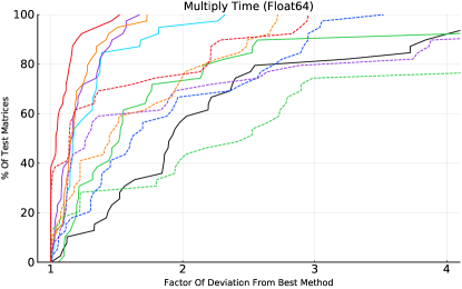
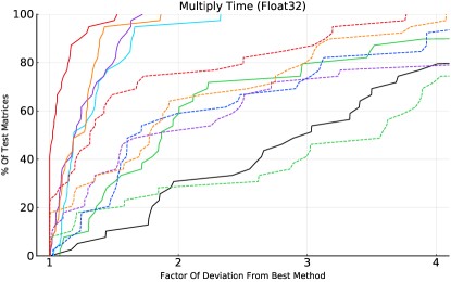
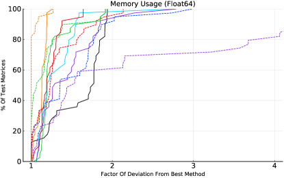
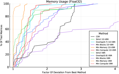
Figure 2: Performance profiles of sparse matrix-vector multiplication time, memory usage, and critical points for our partitioners on our entire test set. The $x$ axis shows the factor of deviation from the best performing partitioner and format, and the $y$ axis shows the percentage of test cases achieving such a factor.

Partitioner		Memory Used				Multiply Time				Critical Point
		Q. 1	Med.	Q. 3		Q. 1	Med.	Q. 3		Q. 1	Med.	Q. 3
Strict 1D-VBR		$0.6$	$0.808$	$1$		$0.573$	$0.886$	$1.17$		$6.57$	$46.1$	$\infty$
Overlap(0.9) 1D-VBR		$0.615$	$0.746$	$0.918$		$0.338$	$0.545$	$0.858$		$10.9$	$18.4$	$68.3$
Overlap(0.8) 1D-VBR		$0.616$	$0.746$	$0.918$		$0.338$	$0.546$	$0.902$		$11.2$	$18.4$	$92.5$
Overlap(0.7) 1D-VBR		$0.619$	$0.746$	$0.918$		$0.331$	$0.547$	$0.904$		$10.9$	$19$	$69$
Min Blocks 1D-VBR		$0.606$	$0.84$	$1.32$		$0.351$	$0.493$	$0.806$		$13.9$	$19$	$66.3$
Min Memory 1D-VBR		$0.562$	$0.633$	$0.806$		$0.347$	$0.535$	$0.723$		$11.7$	$17.3$	$32.2$
Min Compute 1D-VBR		$0.585$	$0.664$	$0.857$		$0.317$	$0.45$	$0.589$		$12.4$	$16.9$	$29.1$
Strict VBR		$0.521$	$0.696$	$0.983$		$0.543$	$1.55$	$2.16$		$29.9$	$\infty$	$\infty$
Overlap(0.9) VBR		$0.575$	$0.819$	$1.18$		$0.508$	$0.769$	$1.52$		$28.8$	$71.4$	$\infty$
Overlap(0.8) VBR		$0.59$	$0.834$	$1.19$		$0.487$	$0.729$	$1.56$		$28.7$	$68$	$\infty$
Overlap(0.7) VBR		$0.605$	$0.847$	$1.2$		$0.501$	$0.777$	$1.55$		$28.5$	$79.2$	$\infty$
Min Blocks VBR		$0.67$	$1.06$	$2.8$		$0.411$	$0.573$	$1.81$		$29$	$47.1$	$\infty$
Min Memory VBR		$0.432$	$0.56$	$0.75$		$0.451$	$0.6$	$1.31$		$38.9$	$62.1$	$\infty$
Min Compute VBR		$0.556$	$0.721$	$1.06$		$0.33$	$0.512$	$1.11$		$36.2$	$49.7$	$\infty$

Table 2: The distribution of the normalized memory usage, multiply time, and critical point (9.9) over each matrix, transposition, and precision in our test set of matrices. A critical point of $\infty$ indicates that no speedup was observed. All metrics are normalized to unpartitioned CSR representation. The “Q. 1”, “Med”, and “Q. 3”, columns refer to the least quartile, median, and greatest quartile, respectively, of the corresponding distribution. The three partitioners with “Min” objectives and the 1D-VBR format are contributions of this work.

Our results show that for both VBR and 1D-VBR, using Algorithm 7 to optimize memory usage or multiplication time consistently produces smaller or faster VBR and 1D-VBR formats than any other partitioner, respectively. Practitioners using variably blocked formats in practice can expect to see improved compression or performance simply by switching to our improved partitioning algorithm to split the matrix, though they may need to use different cost models depending on their application.

The 1D-VBR format is the more performant choice, while VBR is capable of better compression. Using heuristics to partition for 1D-VBR often resulted in faster matrix multiplication than the best VBR partitions. The superior performance of 1D-VBR is due to implementation differences between the two formats. All blocks in a 1D-VBR block row are the same size, but each VBR block requires a random access to the column partition $\Phi$, and a conditional jump to the appropriate block width. Our memory minimizing partitioner was unmatched by any other partitioner for compressing either format, but using this partitioner on VBR format usually yielded the highest compression.

While the heuristics produced quality partitions on some matrices, minimizing our cost models was effective on the entire test set, evinced by the superior third quartile of memory usage and multiplication time for the “Min Memory” and “Min Compute” partitioners. A disadvantage of the overlap heuristic is the need to set the $\rho$ parameter. We plotted values which worked well in our tests, but it may be necessary to test several settings to find the best one, an expensive process [58].

When the precision is reduced, the reference CSR implementation deviates more from the best (blocked) method. Thus, we can say that the benefits of blocking are amplified when the precision is halved. Performance improves because our vector units fit twice the elements, and compression improves because the 64-bit integer indices become twice as large as the individual elements, so there is more incentive to merge blocks. We expect these trends to continue for further reduced precisions, especially when the index precision remains the same.

Our dynamic programming algorithm was similarly efficient to other heuristics. The distribution of critical points shows that the benefits of partitioning outweighed the runtime of partitioning and conversion within a similar number of multiplications. However, the simplicity of the “Strict” heuristic and its specialized conversion to 1D-VBR format made it a practical choice in cases where the matrix had clear blocks. The critical points also show the added partitioning and conversion costs and reduced performance of VBR format, only breaking even after triple the multiplications.

10 Conclusions

We present an algorithm for optimally partitioning rows in a VBR matrix when the columns are fixed. We apply the algorithm to a novel specialization of VBR where only rows are blocked, 1D-VBR. Our algorithm effectively optimizes partitions under a diverse family of cost models. We show that minimizing an empirical cost model for SpMV runtime in 1D-VBR format yields the best performance, and minimizing a cost model for memory consumption in VBR format yields the best compression. The benefits of blocking are amplified as the precision is reduced.

Existing algorithms using variably blocked formats stand to benefit from employing these techniques to pick better partitions, without any changes to the algorithms themselves. Since simultaneous partitioning of rows and columns for VBR format is NP-hard and 1D-VBR is faster and supports diverse cost models, practitioners using two-dimensional aligned block algorithms should consider one-dimensional reformulations when possible.

We hope to see our techniques applied to new cost models and contiguous partitioning problems, such as block decompositions with sparse blocks [47, 48, 50, 51].

A Finding Optimal VBR Partitions is NP-Hard

In this section, we show that Problem 5.1, finding the row and column partition which maximizes a cost model $f(A,\Pi,\Phi)$ of the VBR representation of some matrix $A$, is NP-Hard by reduction from the Maximum Cut problem, one of Karp’s 21 NP-Complete problems [19, 20].

We restate the Maximum Cut problem here for convenience.

Definition A.1 (Maximum Cut)

Given an undirected graph $G=(V,E)$ with $m$ nodes and $n$ edges, split $V$ into two sets $C_{1}\subset V$ and $C_{2}\subset V$ where $C_{1}\cap C_{2}=\emptyset$ and the number of edges between $C_{1}$ and $C_{2}$ is maximized.

Theorem A.1

Problem 5.1 is NP-Hard for any $u_{\max}\geq 2$ and $w_{\max}\geq 2$ and cost functions of the form

(5.7) $$f(A,\Pi,\Phi)=s\cdot N_{\text{index}}+N_{\text{value}}$$

where $s\geq 1$ is constant.

• Assume we are given an instance of Maximum Cut (Problem A.1). We first define a matrix $A$ in terms of $G$ and $s$, then show a correspondence between a class of partitions of $A$ and cuts in $G$. Finally, we show that the $\Pi$ and $\Phi$ which optimize (5.7) correspond to a maximum cut through $G$.

  Let $A$ be an $\mu m\times\mu n$ matrix of zeros and nonzeros, where nonzeros are represented with $x$. Unless stated otherwise, entries of $A$ are defined to be zero. Fix an ordering of the edges of $G$, and let $e_{j}=(i_{1},i_{2})$ where $i_{1}<i_{2}$ be the $j^{th}$ edge in this ordering of $G$. We will insert a $\mu\times\mu$ gadget into $A$ at each endpoint of $e_{j}$, where

  (A.1) $$\mu =3+\mu_{1}+(1+\mu_{1})\mu_{2}+2(1+\mu_{1})\mu_{3}$$

  (A.2) $$\mu_{1} =\lfloor s+1\rfloor$$

  (A.3) $$\mu_{2} =32$$

  (A.4) $$\mu_{3} =\lceil 28s-10\rceil$$

  These constants depend on the relative weights that $s$ assigns to each block and the size of each block. They are larger to make the proof shorter; making them large allows us to upper bound $\mu_{3}$ by $28s-9$ when calculating the cost of each gadget. To give an example of some smaller constants, if $s=1$, we can use $\mu_{1}=2,\mu_{2}=3,\mu_{3}=1$.

  If we think of $A$ as being tiled with $\mu\times\mu$ tiles, the placement of these tiles is analogous to the incidence matrix representation of $G$, so that rows of tiles correspond to vertices and columns of tiles correspond to edges. We insert the gadget $B_{1}$ at the intersection of the $i_{1}^{th}$ tile row and $j^{th}$ tile column.

  $$B_{1}=\left[\begin{array}[]{cccccccccc}x&&&\cdots&x&\cdots&x&\cdots&&\cdots\\ &x&&\cdots&x&\cdots&&\cdots&&\cdots\\ &&x&\cdots&x&\cdots&&\cdots&x&\cdots\\ \vdots&\vdots&\vdots&&&&&&&\\ x&x&x&&&&&&\\ \vdots&\vdots&\vdots&&&&&&&\\ x&&&&&&&&&\\ \vdots&\vdots&\vdots&&&&&&&\\ &&x&&&&&&&\\ \vdots&\vdots&\vdots&&&&&&&\\ \end{array}\right]$$

  We insert the gadget $B_{2}$ at the intersection of the $i_{2}^{th}$ tile row and $j^{th}$ tile column.

  $$B_{2}=\left[\begin{array}[]{cccccccccc}&&x&\cdots&x&\cdots&x&\cdots&&\cdots\\ &x&&\cdots&x&\cdots&&\cdots&&\cdots\\ x&&&\cdots&x&\cdots&&\cdots&x&\cdots\\ \vdots&\vdots&\vdots&&&&&&&\\ x&x&x&&&&&&\\ \vdots&\vdots&\vdots&&&&&&&\\ x&&&&&&&&&\\ \vdots&\vdots&\vdots&&&&&&&\\ &&x&&&&&&&\\ \vdots&\vdots&\vdots&&&&&&&\\ \end{array}\right]$$

  where the upper left patterns occur once, the patterns second to the right and the bottom are repeated $\mu_{2}$ times, and the two rightmost and bottommost patterns are repeated $\mu_{3}$ times. All patterns are followed by $\mu_{1}$ rows or columns of zeros. Figure LABEL:fig:biggadgetmatrix gives an example of $A$ for some $G$.

  The gadgets are identical except for the upper left $3\times 3$ pattern. Thus, the patterns on the top of the gadgets are column-aligned and the patterns on the left are row-aligned across gadget rows and gadget columns. We refer to the resulting fully zero $\mu_{1}$ rows (resp. columns) as filler rows (resp. columns).

  We start by arguing that it is never optimal to produce a partition with a row part that contains both filler rows and non-filler rows. A symmetric argument holds for the columns.

  First, consider the case where the row part contains filler rows on the top or bottom. Separating these rows from the part reduces the sizes $N_{\text{value}}$ of the blocks in that part without changing the number $N_{\text{index}}$ of blocks, so the part cannot have been optimal.

  Second, if the row part does not start or end with a filler row, it must contain filler rows. Since the filler rows in $A$ occur in contiguous groups of size $\mu_{1}$, this part must contain such a group. Consider a block in this part. If the block contains nonzeros on only one side of the filler rows, then separating the rows strictly reduces the size of the block without adding any new blocks. If the block contains nonzeros on both sides of the filler rows, then removing the rows creates a block, but deletes at least $\mu_{1}$ explicitly stored zero values. Since $\mu_{1}>s$, separating these filler rows still reduces the cost of the partition, so it cannot have been optimal.

  Therefore, optimal partitions do not merge different patterns together. We won’t concern ourselves with whether the filler rows have been merged together, since it doesn’t change the cost function. Since the patterns on top consist of only one column, and the patterns on the side consist of only one row, the only undetermined piece of our optimal partition is the partition of the first three rows and columns of each gadget row and gadget column, respectively.

  There remains only four cases for the rows. Either each row lies in a separate part, all rows share a part, the first two rows share a part, or the last two rows share a part. A symmetric argument holds for the columns.

  Sections LABEL:app:vbrblockingnphard:happygadget and LABEL:app:vbrblockingnphard:sadgadget exhaustively check that for all cases where both the first three rows and columns of a gadget have two parts each ($\Pi,\Phi\in\{[1{:}1,2{:}3,...],[1{:}2,3{:}3,...]\}$),

  (A.5) $$f(B_{1},\Pi,\Phi)\leq 146+263s+112s^{2}$$

  and that in all the other cases,

  (A.6) $$f(B_{1},\Pi,\Phi)\geq 147+263s+112s^{2}$$

  The exhaustive proofs for $B_{2}$ are symmetric, so we omit them.

  Assume we start with a row and column partition where only the first three rows and columns of each gadget share parts in the partition. For every row or column part with three members, we split off one row or column into a different part. For any case where the first three rows or columns of a gadget row or column all belong to different parts, we merge two of the rows or columns. For every gadget in our initial partition whose first three rows and columns had two parts each, it’s blocks will be unchanged. For every other gadget, the cost will be strictly reduced. Thus, optimal partitions only merge pairs of rows and columns, and these pairs occur in the first three rows or columns of each gadget row or column. In this case, the cost of every subassembly is the same except for the upper left $3\times 3$ pattern of each gadget. Therefore, the remainder of the argument focuses on these assemblies.

  At this point, we can establish a correspondence between cuts in the graph and partitions. Let $(C_{1},C_{2})$ be a cut in the graph. We will define a row partition $\Pi$ corresponding to this cut. Unless stated otherwise, rows in this partition are assigned to distinct parts. If a vertex $i$ lies in $C_{1}$, then we merge the first and second rows of the corresponding gadget row. If our vertex $i$ lies in $C_{2}$, then we merge the second and third rows of the gadget row. Consider the gadgets corresponding to an edge $e_{j}=(i_{1},i_{2})$. Notice that if vertices $i_{1}$ and $i_{2}$ lie in the same part, $C_{1}$ for example, we have one of the following situations:

  $$vi∈V1Π=[1:2,3:3][x00xx]vi′∈V1Π=[1:2,3:3][00x0x0x0]ej,Φ=[1:2,3:3] or [x000x00x][0xx0x]ej,Φ=[1:1,2:3]Thecostofeitherarrangementisf = 13 + 5s.However,ifverticesi_1andi_2lieindifferentparts,C_1andC_2,forinstance,thesituationisasfollows:vi∈V1Π=[1:2,3:3][x00xx]vi′∈V2Π=[1:1,2:3][x0xx0]ej,Φ=[1:2,3:3] or [x000x00x][0x0x0x00]ej,Φ=[1:1,2:3]Sincethesearetheonlytwogadgetsinthecolumncorrespondingtothisedge,wearefreetochooseacolumnpartition.Theabovepartitionofminimalcosthasacostoff = 10 + 4s,lessthanthecasewheretheverticessharedanedge.Thus,thecostofanoptimalcolumnpartitioncorrespondingtotherowpartitionrepresentationofacutcanbeexpressedasaconstantminus3 + stimesthenumberofcutedges.Sincethereisabijectionbetweencutsandour``pairwise′′rowpartitions(oneofwhichweknowtobeoptimal),producinganoptimalpartitionofrowsandcolumnsisequivalenttofindingthemaximumcutinG.Ifwetreatsasaconstant,ourreductionimposesonlyaconstantfactorofoverheadinmandn,andProblemA.1isreducibletoProblem5.1inpolynomialtime. Figure 33Figure 3G=1234A=[x0xxxxx0xxxxx0xxxx0xxxx00xxxx00xxxx0xxxxxxxxxxxxxxxxxxxxxxxxxxxxxxxxxxxxxxxxxxx0x0x0xxxxxxxxxxxxx0xxxx0x0xxx0x0xxxx0xxxxxxxxxxxxxxxxxxxxxxxx0xx0xxxxxx0xxxxx0xxxx00x0xxx0x0xxxxx00xxxxxxxxxxxxxxxxxxxxxxx0xx0xxxxxx0xxxx0x0xxxxxxxxxxxxxx0x]3Anexampleofoufragmentsfragmentsvi∈V1Π=[1:2,3:3]fragments[missing-subexpressionmissing-subexpressionmissing-subexpressionmissing-subexpressionmissing-subexpressionmissing-subexpression𝑥0missing-subexpression0𝑥missing-subexpressionmissing-subexpressionmissing-subexpressionmissing-subexpressionmissing-subexpressionmissing-subexpressionmissing-subexpressionmissing-subexpressionmissing-subexpressionmissing-subexpressionmissing-subexpressionmissing-subexpression𝑥]missing-subexpressionmissing-subexpressionfragmentsvi′∈V1Π=[1:2,3:3]fragments[missing-subexpressionmissing-subexpressionmissing-subexpressionmissing-subexpressionmissing-subexpressionmissing-subexpressionmissing-subexpressionmissing-subexpressionmissing-subexpression00𝑥0𝑥0missing-subexpressionmissing-subexpressionmissing-subexpressionmissing-subexpressionmissing-subexpressionmissing-subexpressionmissing-subexpressionmissing-subexpressionmissing-subexpression𝑥0missing-subexpressionmissing-subexpressionmissing-subexpressionmissing-subexpression]missing-subexpressionmissing-subexpressionmissing-subexpressionfragmentse𝑗,Φ[1:2,3:3] or fragments[missing-subexpressionmissing-subexpressionmissing-subexpressionmissing-subexpressionmissing-subexpressionmissing-subexpressionmissing-subexpressionmissing-subexpressionmissing-subexpression𝑥000𝑥0missing-subexpressionmissing-subexpressionmissing-subexpressionmissing-subexpressionmissing-subexpressionmissing-subexpressionmissing-subexpressionmissing-subexpressionmissing-subexpressionmissing-subexpression0𝑥missing-subexpressionmissing-subexpressionmissing-subexpression]missing-subexpressionfragments[missing-subexpressionmissing-subexpressionmissing-subexpressionmissing-subexpressionmissing-subexpressionmissing-subexpressionmissing-subexpression0𝑥missing-subexpression𝑥0missing-subexpressionmissing-subexpressionmissing-subexpressionmissing-subexpressionmissing-subexpressionmissing-subexpressionmissing-subexpressionmissing-subexpressionmissing-subexpression𝑥missing-subexpressionmissing-subexpression]missing-subexpressionfragmentse𝑗,Φ[1:1,2:3]Thecostofeitherarrangementisf = 13 + 5s.However,ifverticesi_1andi_2lieindifferentparts,C_1andC_2,forinstance,thesituationisasfollows:vi∈V1Π=[1:2,3:3][x00xx]vi′∈V2Π=[1:1,2:3][x0xx0]ej,Φ=[1:2,3:3] or [x000x00x][0x0x0x00]ej,Φ=[1:1,2:3]Sincethesearetheonlytwogadgetsinthecolumncorrespondingtothisedge,wearefreetochooseacolumnpartition.Theabovepartitionofminimalcosthasacostoff = 10 + 4s,lessthanthecasewheretheverticessharedanedge.Thus,thecostofanoptimalcolumnpartitioncorrespondingtotherowpartitionrepresentationofacutcanbeexpressedasaconstantminus3 + stimesthenumberofcutedges.Sincethereisabijectionbetweencutsandour``pairwise′′rowpartitions(oneofwhichweknowtobeoptimal),producinganoptimalpartitionofrowsandcolumnsisequivalenttofindingthemaximumcutinG.Ifwetreatsasaconstant,ourreductionimposesonlyaconstantfactorofoverheadinmandn,andProblemA.1isreducibletoProblem5.1inpolynomialtime. Figure 33Figure 3G=1234A=[x0xxxxx0xxxxx0xxxx0xxxx00xxxx00xxxx0xxxxxxxxxxxxxxxxxxxxxxxxxxxxxxxxxxxxxxxxxxx0x0x0xxxxxxxxxxxxx0xxxx0x0xxx0x0xxxx0xxxxxxxxxxxxxxxxxxxxxxxx0xx0xxxxxx0xxxxx0xxxx00x0xxx0x0xxxxx00xxxxxxxxxxxxxxxxxxxxxxx0xx0xxxxxx0xxxx0x0xxxxxxxxxxxxxx0x]3Anexampleofou$$

References

- [1] Yousef Saad. Iterative methods for sparse linear systems. SIAM, Philadelphia, 2nd edition, 2003.
- [2] Richard Vuduc, James W Demmel, and Katherine A Yelick. OSKI: A library of automatically tuned sparse matrix kernels. Journal of Physics: Conference Series, 16:521–530, January 2005.
- [3] Timothy A. Davis, Sivasankaran Rajamanickam, and Wissam M. Sid-Lakhdar. A survey of direct methods for sparse linear systems. Acta Numerica, 25:383–566, May 2016. Publisher: Cambridge University Press.
- [4] James W. Demmel, Stanley C. Eisenstat, John R. Gilbert, Xiaoye S. Li, and Joseph W. H. Liu. A Supernodal Approach to Sparse Partial Pivoting. SIAM Journal on Matrix Analysis and Applications, 20(3):720–755, January 1999. Publisher: Society for Industrial and Applied Mathematics.
- [5] Yousef Saad. Finding Exact and Approximate Block Structures for ILU Preconditioning. SIAM Journal on Scientific Computing, 24(4):1107–1123, January 2003.
- [6] Ichitaro Yamazaki, Sivasankaran Rajamanickam, and Nathan Ellingwood. Performance Portable Supernode-based Sparse Triangular Solver for Manycore Architectures. In 49th International Conference on Parallel Processing - ICPP, ICPP ’20, pages 1–11, New York, NY, USA, August 2020. Association for Computing Machinery.
- [7] Cleve Ashcraft and Roger Grimes. The influence of relaxed supernode partitions on the multifrontal method. ACM Transactions on Mathematical Software, 15(4):291–309, December 1989.
- [8] Kyungjoo Kim, Sivasankaran Rajamanickam, George Widgery Stelle, Harold C. Edwards, and Stephen Lecler Olivier. Task Parallel Incomplete Cholesky Factorization using 2D Partitioned-Block Layout. Technical Report SAND-2016-0637R, Sandia National Lab. (SNL-NM), Albuquerque, NM (United States), January 2016.
- [9] Richard W. Vuduc and Hyun-Jin Moon. Fast Sparse Matrix-Vector Multiplication by Exploiting Variable Block Structure. In Laurence T. Yang, Omer F. Rana, Beniamino Di Martino, and Jack Dongarra, editors, High Performance Computing and Communications, Lecture Notes in Computer Science, pages 807–816, Berlin, Heidelberg, 2005. Springer.
- [10] V. Karakasis, G. Goumas, and N. Koziris. Perfomance Models for Blocked Sparse Matrix-Vector Multiplication Kernels. In 2009 International Conference on Parallel Processing, pages 356–364, September 2009.
- [11] Vasileios Karakasis, Georgios Goumas, and Nectarios Koziris. A Comparative Study of Blocking Storage Methods for Sparse Matrices on Multicore Architectures. In 2009 International Conference on Computational Science and Engineering, pages 247–256, Vancouver, BC, Canada, 2009. IEEE.
- [12] Youcef Saad. SPARSKIT: A basic tool kit for sparse matrix computations. Technical report, May 1990.
- [13] Youcef Saad. SPARSKIT: a basic tool kit for sparse matrix computations - Version 2. 1994.
- [14] Karin Remington and Roldan Pozo. NIST Sparse BLAS: User’s Guide. Technical report, NIST, 1996.
- [15] Richard W. Vuduc. Automatic performance tuning of sparse matrix kernels. PhD thesis, University of California, Berkeley, CA, USA, January 2004.
- [16] Developer Reference for Intel® Math Kernel Library - Fortran. Technical Report 097, Intel®, 2020.
- [17] Manu Shantharam, Anirban Chatterjee, and Padma Raghavan. Exploiting dense substructures for fast sparse matrix vector multiplication. The International Journal of High Performance Computing Applications, 25(3):328–341, August 2011.
- [18] Ali Pinar and Michael T. Heath. Improving Performance of Sparse Matrix-vector Multiplication. In Proceedings of the 1999 ACM/IEEE Conference on Supercomputing, SC ’99, New York, NY, USA, 1999. ACM. event-place: Portland, Oregon, USA.
- [19] Richard M. Karp. Reducibility among Combinatorial Problems. In Raymond E. Miller, James W. Thatcher, and Jean D. Bohlinger, editors, Complexity of Computer Computations: Proceedings of a symposium on the Complexity of Computer Computations, held March 20–22, 1972, at the IBM Thomas J. Watson Research Center, Yorktown Heights, New York, and sponsored by the Office of Naval Research, Mathematics Program, IBM World Trade Corporation, and the IBM Research Mathematical Sciences Department, The IBM Research Symposia Series, pages 85–103. Springer US, Boston, MA, 1972.
- [20] Christos H. Papadimitriou and Mihalis Yannakakis. Optimization, approximation, and complexity classes. Journal of Computer and System Sciences, 43(3):425–440, December 1991.
- [21] Alfredo Buttari, Victor Eijkhout, Julien Langou, and Salvatore Filippone. Performance Optimization and Modeling of Blocked Sparse Kernels. The International Journal of High Performance Computing Applications, 21(4):467–484, November 2007.
- [22] Anael Grandjean, Johannes Langguth, and Bora Uçar. On Optimal and Balanced Sparse Matrix Partitioning Problems. In 2012 IEEE International Conference on Cluster Computing, pages 257–265, September 2012. ISSN: 2168-9253.
- [23] Brad Jackson, Jeffrey D. Scargle, David Barnes, Sundararajan Arabhi, Alina Alt, Peter Gioumousis, Elyus Gwin, Paungkaew Sangtrakulcharoen, Linda Tan, and Tun Tao Tsai. An Algorithm for Optimal Partitioning of Data on an Interval. IEEE Signal Processing Letters, 12(2):105–108, February 2005. arXiv: math/0309285.
- [24] C.J. Alpert and A.B. Kahng. Multiway partitioning via geometric embeddings, orderings, and dynamic programming. IEEE Transactions on Computer-Aided Design of Integrated Circuits and Systems, 14(11):1342–1358, November 1995.
- [25] Louis H. Ziantz, Can C. Özturan, and Boleslaw K. Szymanski. Run-time optimization of sparse matrix-vector multiplication on SIMD machines. In Costas Halatsis, Dimitrios Maritsas, George Philokyprou, and Sergios Theodoridis, editors, PARLE’94 Parallel Architectures and Languages Europe, Lecture Notes in Computer Science, pages 313–322, Berlin, Heidelberg, 1994. Springer.
- [26] Brian W. Kernighan. Optimal Sequential Partitions of Graphs. Journal of the ACM (JACM), 18(1):34–40, January 1971.
- [27] Tamara G. Kolda. Partitioning sparse rectangular matrices for parallel processing. In Alfonso Ferreira, José Rolim, Horst Simon, and Shang-Hua Teng, editors, Solving Irregularly Structured Problems in Parallel, Lecture Notes in Computer Science, pages 68–79, Berlin, Heidelberg, 1998. Springer.
- [28] Bruce Hendrickson and Tamara G. Kolda. Graph Partitioning Models for Parallel Computing. Parallel Comput., 26(12):1519–1534, November 2000.
- [29] Abdurrahman Yaşar and Ümit V. Çatalyürek. Heuristics for Symmetric Rectilinear Matrix Partitioning. arXiv:1909.12209 [cs], September 2019. arXiv: 1909.12209.
- [30] R. Vuduc, J.W. Demmel, K.A. Yelick, S. Kamil, R. Nishtala, and B. Lee. Performance Optimizations and Bounds for Sparse Matrix-Vector Multiply. pages 26–26. IEEE, 2002.
- [31] Javed Razzaq, Rudolf Berrendorf, Jan P. Ecker, Soenke Hack, Max Weierstall, and Florian Manuss. The DynB Sparse Matrix Format Using Variable Sized 2D Blocks for Efficient Sparse Matrix Vector Multiplications with General Matrix Structures. International Journal On Advances in Intelligent Systems, 10(1 and 2):48–58, June 2017.
- [32] Eun-Jin Im. Optimizing the Performance of Sparse Matrix-Vector Multiplication. PhD thesis, EECS Department, University of California, Berkeley, June 2000.
- [33] Eun-Jin Im and Katherine Yelick. Optimizing Sparse Matrix Computations for Register Reuse in SPARSITY. In Computational Science — ICCS 2001, Lecture Notes in Computer Science, pages 127–136. Springer, Berlin, Heidelberg, May 2001.
- [34] Eun-Jin Im, Katherine Yelick, and Richard Vuduc. Sparsity: Optimization Framework for Sparse Matrix Kernels. International Journal of High Performance Computing Applications, 18(1):135–158, February 2004.
- [35] Ryan Eberhardt and Mark Hoemmen. Optimization of Block Sparse Matrix-Vector Multiplication on Shared-Memory Parallel Architectures. In 2016 IEEE International Parallel and Distributed Processing Symposium Workshops (IPDPSW), pages 663–672, May 2016.
- [36] Jee W. Choi, Amik Singh, and Richard W. Vuduc. Model-driven autotuning of sparse matrix-vector multiply on GPUs. ACM SIGPLAN Notices, 45(5):115, May 2010.
- [37] B.C. Lee, R.W. Vuduc, J.W. Demmel, and K.A. Yelick. Performance models for evaluation and automatic tuning of symmetric sparse matrix-vector multiply. pages 169–176 vol.1. IEEE, 2004.
- [38] P. Ahrens, H. Xu, and N. Schiefer. A Fill Estimation Algorithm for Sparse Matrices and Tensors in Blocked Formats. In 2018 IEEE International Parallel and Distributed Processing Symposium (IPDPS), pages 546–556, May 2018.
- [39] Helen Xu. Fill Estimation for Blocked Sparse Matrices and Tensors. PhD thesis, Department of Electrical Engineering and Computer Science, Massachusetts Institute of Technology, June 2018.
- [40] Peter Ahrens. A Parallel Fill Estimation Algorithm for Sparse Matrices and Tensors in Blocked Formats. Thesis, Massachusetts Institute of Technology, 2019.
- [41] Virginia Vassilevska and Ali Pinar. Finding Nonoverlapping Dense Blocks of a Sparse Matrix. February 2004.
- [42] Xinhai Chen, Peizhen Xie, Lihua Chi, Jie Liu, and Chunye Gong. An efficient SIMD compression format for sparse matrix-vector multiplication. Concurrency and Computation: Practice and Experience, 30(23):e4800, 2018.
- [43] Rajesh Nishtala, Richard W. Vuduc, James W. Demmel, and Katherine A. Yelick. When cache blocking of sparse matrix vector multiply works and why. Applicable Algebra in Engineering, Communication and Computing, 18(3):297–311, May 2007.
- [44] A. N. Yzelman. Generalised Vectorisation for Sparse Matrix: Vector Multiplication. In Proceedings of the 5th Workshop on Irregular Applications: Architectures and Algorithms, IA ’15, pages 6:1–6:8, New York, NY, USA, 2015. ACM.
- [45] Fred G. Gustavson. Two Fast Algorithms for Sparse Matrices: Multiplication and Permuted Transposition. ACM Transactions on Mathematical Software (TOMS), 4(3):250–269, September 1978.
- [46] Kevin Aydin, MohammadHossein Bateni, and Vahab Mirrokni. Distributed Balanced Partitioning via Linear Embedding †. Algorithms, 12(8):162, August 2019. Number: 8 Publisher: Multidisciplinary Digital Publishing Institute.
- [47] Aydin Buluc and John R. Gilbert. On the representation and multiplication of hypersparse matrices. In 2008 IEEE International Symposium on Parallel and Distributed Processing, pages 1–11, April 2008. ISSN: 1530-2075.
- [48] Aydin Buluç, Jeremy T. Fineman, Matteo Frigo, John R. Gilbert, and Charles E. Leiserson. Parallel sparse matrix-vector and matrix-transpose-vector multiplication using compressed sparse blocks. page 233. ACM Press, 2009.
- [49] Yunming Zhang, Vladimir Kiriansky, Charith Mendis, Saman Amarasinghe, and Matei Zaharia. Making caches work for graph analytics. In 2017 IEEE International Conference on Big Data (Big Data), pages 293–302, December 2017.
- [50] Changwan Hong, Aravind Sukumaran-Rajam, Israt Nisa, Kunal Singh, and P. Sadayappan. Adaptive Sparse Tiling for Sparse Matrix Multiplication. In Proceedings of the 24th Symposium on Principles and Practice of Parallel Programming, PPoPP ’19, pages 300–314, New York, NY, USA, February 2019. Association for Computing Machinery.
- [51] Naveen Namashivayam, Sanyam Mehta, and Pen-Chung Yew. Variable-Sized Blocks for Locality-Aware SpMV. In Proc. of the Annual IEEE/ACM Int’l Symp. on Code Generation and Optimization (CGO), Virtual Event, Seoul, March 2021.
- [52] W.A. Greene. k-way merging and k-ary sorts. In [Proceedings] 1991 Symposium on Applied Computing, pages 197–, April 1991. ISSN: null.
- [53] J. Bezanson, A. Edelman, S. Karpinski, and V. Shah. Julia: A Fresh Approach to Numerical Computing. SIAM Review, 59(1):65–98, January 2017.
- [54] IEEE Standard for Floating-Point Arithmetic. IEEE Std 754-2019 (Revision of IEEE 754-2008), pages 1–84, July 2019.
- [55] Erik Schnetter, Takafumi Arakaki, Valentin Churavy, Kristoffer Carlsson, Nicolau Leal Werneck, Steve Kelly, Gunnar Farnebäck, Miguel Raz Guzmán Macedo, Matt Bauman, Kenta Sato, and Elliot Saba. eschnett/SIMD.jl: v2.8.0, July 2019.
- [56] Timothy A. Davis and Yifan Hu. The university of Florida sparse matrix collection. ACM Transactions on Mathematical Software, 38(1):1–25, November 2011.
- [57] Elizabeth D. Dolan and Jorge J. Moré. Benchmarking optimization software with performance profiles. Mathematical Programming, 91(2):201–213, January 2002.
- [58] R. W. Vuduc and H. Moon. Fast sparse matrix-vector multiplication by exploiting variable block structure. Technical Report UCRL-TR-213454, Lawrence Livermore National Lab. (LLNL), Livermore, CA (United States), July 2005.