MNRAS LaTeX 2ε template – title goes here

Simulating the outer layers of rapidly rotating stars

Abstract

This paper presents the results of a set of radiative hydrodynamic (RHD) simulations of convection in the near-surface regions of a rapidly rotating star. The simulations use microphysics consistent with stellar models, and include the effects of realistic convection and radiative transfer. We find that the overall effect of rotation is to reduce the strength of turbulence. The combination of rotation and radiative cooling creates a zonal velocity profile in which the motion of fluid parcels near the surface is independent of rotation. Their motion is controlled by the strong up and down flows generated by radiative cooling. The fluid parcels in the deeper layers, on the other hand, are controlled by rotation.

1 Introduction

Convection is one of the two dominant forms of heat transport in stars, and is also a significant source of uncertainty in stellar models. These models are predominantly one-dimensional, and incorporating a three-dimensional (3D) phenomenon such as convection into them, requires drastic approximations, such as the mixing length approximation (MLT) Böhm-Vitense (1958). While MLT is successful in reproducing the properties of stars in near-adiabatic regions of efficient convection, there is evidence from helioseismic and asteroseismic observations that these approximations do not model the near-surface layers of a star particularly well (Abbett et al., 1997; Kim et al., 1996). Of much more concern is the fact that the free parameters in the approximation directly control the radii of models, and thus these models cannot predict stellar radii without introducing additional constraints. To overcome this constraint, there are increasing efforts to simulate convection in the outer regions of stars on different parts of the Hertzsprung-Russell (HR) diagram (Magic et al., 2013c; Trampedach et al., 2013a) for different metallicity (Magic et al., 2013a; Tanner et al., 2013) in order understand near-surface convection, and also to use the results of the simulations to improve stellar models (Mosumgaard et al., 2018; Spada et al., 2018). These studies of convection have generally been limited to non-rotating stars. In this work we explore how rapid rotation affects near-surface convection.

Stellar convection has a huge range of spatial and temporal scales making it impossible to resolve all the dynamical and thermal scales in a numerical model. Consequently, there have been two approaches to modeling convection in stars; (i) global models of all or a large part of a star or (ii) local models of the surface layers of a tiny part of the star.

Global models have been developed for the Sun to model differential rotation (Brun & Toomre, 2002; Miesch, 2007), meridional circulation (Featherstone & Miesch, 2015) and the near-surface shear layer (Miesch & Hindman, 2011; Hotta et al., 2014). More recently, these techniques have been applied to other types of stars (Palacios & Brun, 2007; Brun et al., 2017). These models typically include the entire convection zone in a full spherical shell geometry (Miesch et al., 2006; Brun et al., 2011; Nelson et al., 2018), solving a truncated form of the fully compressible system called the anelastic approximation. In this approximation, acoustic waves are filtered out and a linearized form of the governing equations is solved (see Appendix). This approximation limits the simulations to regions of efficient convection, and is therefore not suitable to study the effects of inefficient convection that causes the greatest uncertainty in stellar models. Other global models (Robinson & Chan, 2001; Käpylä et al., 2010), solve the fully compressible system in a wedge covering 60-120 degrees in latitude and longitude centered about the equator.

The global models span about 6-8 scale heights, whereas the convection zone on encompasses about 19 pressure scale heights. This means that the resolved eddies in the global simulations are thousands of times larger than solar granules observed at the surface of the Sun,and hence again not suitable for studying the effects of inefficient convection on stellar structure. Furthermore, the numerical energy flux at the lower boundary is millions of times larger than the actual radiative flux at that depth (Brandenburg et al., 2005). In these models the equation of state is typically an ideal gas and radiation is approximated by a conduction layer (Brun & Toomre, 2002).

Local models are designed to accurately represent energy transport in the thin convection-radiation transition layer at the top of the star. Nordlund (1985) was among the first to use local RHD simulations to accurately account for realistic near-surface convective dynamics and radiative energy transport, but the technique has since been used by numerous authors (e.g. Chan & Sofia, 1989; Freytag & Steffen, 2004; Magic et al., 2013b). These type of simulations are 3D Radiation Hydrodynamic (3DRHD) simulations and, as the name suggests, includes the effect radiation has on the dynamics caused by convection. Typically, the depth of a simulation box is between 3 and 5 Mm (about 8 pressure scale heights). The simulation is driven by an imposed energy flux at the base of the box. In these ‘realistic’ simulations, this energy flux is close to the radiative flux $\sigma{{\rm T}_{\rm eff}}^{4}$, whereas in the global simulation it is many times larger. The simulations use realistic equations of state $P(\rho,e)$, where $P$, $\rho$ and $e$ are the pressure, density and internal energy of the gas, respectively. They also include the thermodynamic effects of ionization zones and use full radiative transfer (Stein & Nordlund, 2000; Freytag et al., 2012; Trampedach et al., 2013b). The majority of 3DRHD simulations have been of the Sun and other solar-like stars (Robinson et al., 2003; Beeck et al., 2012; Tanner et al., 2016; Chiavassa et al., 2018; Collet et al., 2007), but there have also been realistic simulations of Subgiants (Robinson et al., 2004), M-Dwarfs (Ludwig et al., 2002; Wedemeyer et al., 2013),Betelgeuse (Freytag et al., 2002), F stars such as Procyon (Robinson et al., 2005) and others (Kitiashvili et al., 2016).

While the global models must include the effects of rotation, the local models of "realistic convection" typically do not. This is because for most stars being studied (Mathur et al., 2011), the convective timescales in the computational domain are tiny compared to the rotation period of the star. For example, solar granules have lifetimes of about 10 minutes, while the Sun takes 25 days to spin once. The importance of rotation associated with such flow, can be estimated from the ratio of this turnover time to the rotation period, which for solar granules is about $3\times 10^{-4}$. Under such conditions the Coriolis terms in the Navier-Stokes equations will be insignificant compared to the other momentum terms. The importance of the centrifugal force can be estimated by $R\Omega^{2}/g$, where $R$, $\Omega$ and $g$, are the radius, external rotation rate and acceleration due to gravity at the top of the star. For the Sun, this parameter is $\approx 10^{-5}$, so the centrifugal force can also be ignored in local models of the Sun.

If the star is spinning fast enough, granules should start to feel rotation. This paper described a set of simulations of rapidly spinning stars that have rotation periods that are about an order of magnitude greater than the eddy turnover time. As an example, for a simulation of $\delta$-Scuti, the estimated turnover time for a granule is about 30 minutes, while the observed rotation period can be as short as 6 hours (Solano & Fernley, 1997; Molenda-Zakowicz et al., 2009). Under these conditions, rotation cannot be ignored.

2 Model Description

Our numerical code solves the fully compressible Navier-Stokes equations with radiative transfer. Details of the non-rotating version are provided in Tanner et al. (2012, 2016) (and references therein). The code is an updated version of the code used in Robinson et al. (2003, 2004) and is based on the code written by Kim & Chan (1998). Here, we outline its basic ingredients and key features among recent improvements.

A 3D model is characterized by its surface gravity, chemical composition, and effective temperature, although only the former two properties can be directly set in a simulation. To produce a 3D RHD simulation, we begin with a stratification extracted from a 1D stellar model. The initial stratification is taken from a 1D stellar model computed using MLT which is then relaxed to a steady state that is consistent with the realistic convective dynamics and radiative transfer. In this work, we use the 1D stellar evolution code YREC (Demarque et al., 2008) to obtain the initial stratification, but this does not affect the final relaxed state of the simulation, which can be characterized by the chemical composition, surface gravity, and effective temperature. As a result of the inadequacy of MLT, the relaxed state of a 3D RHD simulation is not consistent with the stratification from the initial MLT model, and consequently, the radiative flux may converge to a value that differs from the 1D model. Since it is determined from the radiative flux, the effective temperature is a computed property of a relaxed simulation, and we cannot set this as an input constraint. The simulations presented in this paper are for a $\delta$ Scuti-type star with $\log g$ and $\log{T_{\rm eff}}$ of 4.21 and about 3.81, respectively (the Sun has values of 4.44 and 3.76).

Due to the very large range of scales in a stellar convection zone (e.g. 19 pressure scale heights for the Sun), the computational domain that is used is typically a tiny box, or thin shell, located at the top of the convection zone. The box has a width equal to that of a few granules and is deep enough so that further increases in depth do not alter the flow structure, with the top of the box located at least 1 pressure scale height (${\rm H_{P}}$) above the photosphere. In this region, ${\rm H_{P}}$ is about 500km. The depth of the domain is important because boundary effects can be reduced (though never eliminated) by increasing the vertical extent until quantities within 1 ${\rm H_{P}}$ of the upper and lower boundaries remain unchanged, if further increases are made. The vertical walls are periodic and the horizontal walls are impenetrable (closed box). To help reduce large horizontal velocities (and shocks) in the low density layers near the top of the box, a no-slip boundary condition is imposed at the top of the box, while the bottom of the box is stress free. By comparing different 3D radiation hydrodynamics simulations, Kupka et al. (2005) and Kupka (2008), showed that the effect of the top boundary on the underlying convection is felt only within a pressure scale height of the top. The effect of no-slip versus slippy top was tested for simulations of the Sun in Robinson et al. (2003). It was found that the boundary condition at the top had little impact on the dynamical or thermal structure of the superadiabatic layer. A more recent comparison between the CO5BOLD, MURaM (Vögler et al., 2005) and Stagger codes (Nordlund & Galsgaard, 1995) was made by Beeck et al. (2012). Again, even though the codes use different numerical schemes and the runs are for different resolution, different top boundary conditions and different domain sizes, the dynamical and thermal structure below the photosphere look almost the same.

In the deeper, more opaque regions (optical depth of $\tau>10^{4}$), radiative transfer is modeled by the diffusion approximation. However, in the shallower regions, such as the superadiabatic layer, photon mean free paths are not small enough to use the diffusion approximation. Here $Q_{rad}$, the energy transferred by radiation, is computed as $Q_{\rm rad}=4\kappa\rho(J$-$B)$ where $\kappa$ is the Rosseland mean opacity, and the mean intensity $J$ is computed by using the generalized three-dimensional Eddington approximation of Unno & Spiegel (1966). This formulation is exact for isotropic radiation in a gray atmosphere, and without requiring local thermodynamic equilibrium, the Eddington approximation describes the optically thick and thin regions exactly (Rutten et al., 1995). A detailed comparison between using the 3D Eddington and ray integration for radiation has been done by Tanner et al. (2012) who concluded that as far as convection below the surface is concerned, there are only minor differences in the dynamics or thermal structure between simulations using ray integration or 3D Eddington.

The code is numerically stable for stars with surface gravity similar to that of the Sun or higher surface gravities, as well as somewhat hotter stars like F-type stars; no additional artificial viscosity is needed to stabilize the code. The subgrid-scale model employed is the one from Smagorinsky (1963).

2.1 Adding rotation: the $f$ plane box

To include rotation, we employ the $f$-plane approximation (Pedlosky & Robertson, 1988). In our configuration, $f$ is defined as $2\Omega{\rm sin}\theta$, where $\theta$ is co-latitude. The geometry is shown in Fig. 1.The computational domain can be thought of as a tiny part of a spherical shell at a particular co-latitude. The assumption of constant $f$ is good, provided the box size is small compared to the radius of the star, which is indeed the case of our simulations. In the right handed Cartesian geometry that we use, the $x$ direction is towards the equator, $y$ is in the zonal direction and the $z$ direction is radially outwards. This means gravity $g$ is in the negative $z$ direction).

Figure 1: The $f$-plane geometry.

The $f$-plane configuration has been used to simulate rotating turbulent convection (Brummell et al., 1996; Chan, 2001, 2007), and convectively generated vortices in Jovian planets Chan & Mayr (2013). All of these $f$-plane simulations are for idealised polytropic stratifications with input fluxes many orders of magnitude greater than the solar flux. The current application is different in that it is of realistic surface convection which contains both shallow and deep convection.

2.2 Non-dimensional units

Physical quantities are scaled by their value at a reference level located near the top of the box. For instance, velocity is scaled by the isothermal sound speed, $c_{\rm s}=(p_{\rm top}/\rho_{\rm top})^{1/2}$, and time by $d/c_{\rm s}$, where $d$ is the depth of the box. In such units, the external angular velocity, $\Omega$, is scaled by $c_{\rm s}/d$.

2.3 Centrifugal and Coriolis Forces

Results presented in this paper are for an $f$-plane box located at the equator ($\theta=\pi/2$, $f=2\Omega$). In this configuration, the centrifugal force is in the opposite direction to gravity and can be included by simply subtracting $R\Omega^{2}$ (where $R$ is the radius of the star) from the uniform gravitational acceleration. As ${\bf\Omega}$ points along the $-x$ direction, there will be two non-zero components of the Coriolis force, $-(2\Omega v_{z})\hat{y}$ and $(2\Omega v_{y})\hat{z}$, where $v_{y}$, $v_{z}$, $\hat{y}$ and $\hat{z}$ are the zonal and vertical velocities and unit vectors in the $y$ and $z$ direction, respectively.

2.4 Turbulent fluid properties

Following the notation employed by Chan (2001), any turbulent fluid quantity $q$ can be split into a mean and a fluctuating part,

$$q=\overline{q}(z)+q^{\prime}(x,y,z,t).$$ (1)

The overbar represents a combined horizontal and temporal average, i.e.

$$\overline{q}(z)=\frac{1}{t_{2}-t_{1}}\int\limits_{t_{1}}^{t_{2}}\left(\frac{1}{(L_{x}L_{y})}\int qdxdy\right)dt.$$ (2)

$t_{1}$, is a time after the system has reached a self-consistent thermal equilibrium (the thermal adjustment time). $L_{x}$ and $L_{y}$ are the horizontal widths of the box in the $x$ and $y$ direction respectively. The time required for statistical convergence is $t_{2}-t_{1}$.

The root mean square (r.m.s.) value of a quantity $q$ is defined as

$$q^{\prime\prime}=\overline{q^{2}}-{\overline{q}}^{2},$$ (3)

while the correlation coefficient of two quantities $q_{1}$ and $q_{2}$, is defined as

$$C[q_{1}^{\prime}q_{2}^{\prime}]=\frac{\overline{q_{1}q_{2}}-\overline{q_{1}}\hskip 2.84526pt\overline{q_{2}}}{q_{1}^{\prime\prime}q_{2}^{\prime\prime}}$$ (4)

The symbol $\langle q\rangle$ denotes averaging over the height, $d$, of the box:

$$\langle q\rangle=\frac{1}{d}\int{q}$$ (5)

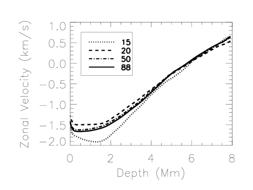
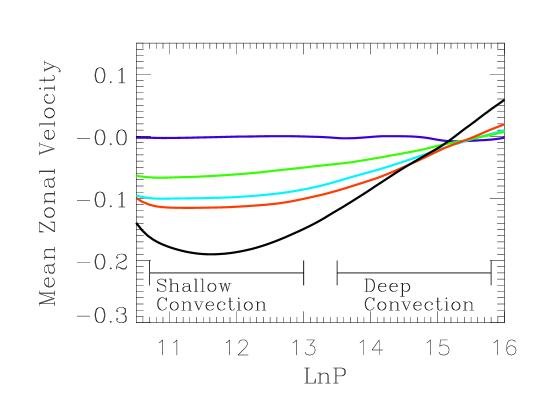
Statistical convergence has been verified by comparing each quantity at different averaging times. If averaging over an additional 10 turnover times, did not change the value of a quantity by more than 1 %, then it was considered converged. For example, the mean zonal velocity in the box, $\overline{v_{y}}$ in case D is shown in Fig. 2. The zonal velocity, $v_{y}=v_{\phi}-R\Omega$, where $v_{\phi}$ is the equatorial tangential velocity at a given point in the star. It has been averaged over 15, 20, 50 and 88 time units. For rotating deep efficient convection, the slope of $\overline{v_{y}}$ should be $-2\Omega$ (Chan, 2001). As the deep layers take longer to converge (due to the longer turnover times), once the slope of $\overline{v_{y}}$ versus depth is constant near the base, one can assume $\overline{v_{y}}$ is close to convergence in the rest of the box.

Figure 2: Convergence of mean zonal velocity, ${\overline{v}_{y}}$. The plot is for case D. Each line represents a different averaging times (in non-dimensional time units). ${\overline{v}_{y}}$ is converged after about 50 time units.

3 Results

Table  1 lists some properties of the simulations. Columns 1-6 are model identifier, rotational velocity $v_{\rm rot}=R\Omega$, non-dimensional angular velocity ${\Omega}^{*}$, relative reduction in $g$ due to centrifugal force, r.m.s. velocity fluctuation and r.m.s. velocity, respectively. The r.m.s. velocity fluctuation is computed as the depth average of $v^{\prime\prime}$, where $v^{\prime\prime}=({{v_{x}}^{\prime\prime}}^{2}+{{v_{y}}^{\prime\prime}}^{2}+{{v_{z}}^{\prime\prime}}^{2})^{1/2}$. The r.m.s. velocity is computed similarly, but without subtracting the mean.

From $v^{\prime\prime}$, various non-dimensional turbulence parameters are computed and presented in columns 7-9. The Coriolis number (inverse Rossby number), Co, is defined as ${\rm Co}=\Omega d/\langle v^{\prime\prime}\rangle$. The Reynolds numbers, Re, which compares the magnitudes of the inertia and viscous terms, is defined as $\langle v^{\prime\prime}\rangle d/\langle\overline{\mu}/\overline{\rho}\rangle$ (where $\mu$ and $\rho$ are the subgrid scale dynamic viscosity and the density). The Taylor number Ta, which compares the Coriolis and viscous terms, is computed as $(2\Omega d^{2}/\langle\overline{\mu}/\overline{\rho}\rangle)^{2}$.

Table 1: Dynamical Characteristics of Simulations

Model	$v_{\rm rot}$ (km/s)	$\Omega^{*}$	$(g-R{\Omega}^{2})/g$	$\langle v^{\prime\prime}\rangle({\rm km/s})$	${\langle{\overline{v}^{2}}\rangle}^{1/2}({\rm km/s})$	Co	Re	Ta
A	0	0.0	1.0	4.72	4.86	0.0	2070	0.0
B	153	0.064	1.0	4.38	4.62	0.21	1760	$5.5\times{10^{5}}$
C	153	0.064	0.9	4.31	4.51	0.21	1810	$6\times{10^{5}}$
D	184	0.089	0.81	4.20	4.47	0.31	1865	$1.3\times{10^{6}}$
E	307	0.128	0.61	3.98	4.42	0.46	1893	$3.1\times{10^{6}}$

3.1 Thermal structure

One measure of convective instability is the superadiabaticity, defined as $\nabla-\nabla_{\rm ad}$ where $\nabla={\rm dlnT/dlnP}$ and $\nabla_{\rm ad}$ is the adiabatic temperature gradient. The total pressure is the sum of the gas, P and turbulent pressure ${\rm P_{turb}}=\overline{\rho}(v_{z}^{\prime\prime})^{2}$. For deep efficient convection, $\nabla-\nabla_{\rm ad}$ is slightly above zero ($\sim 10^{-6}$ in the solar convection zone), while for shallow inefficient convection it is of order unity.

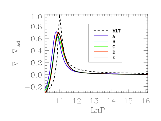
Fig. 3 shows $\nabla-\nabla_{\rm ad}$, plotted against LnP for the stellar model (using MLT) that sets the initial conditions for the 5 simulations described in Table 1. The superadiabaticity from 3D RHD simulations is significantly different than that of the MLT model. This difference is due to the realistic convective and radiative transport near the surface.

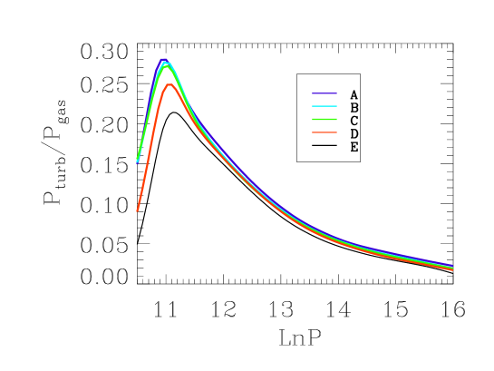
Another characteristic that the MLT approximation of convection does not account for is turbulent pressure. The turbulent pressure as a fraction of by the gas pressure is plotted in Fig. 4 for each of the simulations, while the turbulent pressure for the MLT model is not shown because it is zero.

Comparing the MLT model with simulation A in figure 3, one can see that the turbulent pressure has pushed the superadiabatic layer (SAL) outwards by about 0.5${\rm H}_{\rm P}$ from its original position. The photospheric surface is moved out by a similar amount. Adding rotation reduces the turbulent pressure, so that the SAL is not pushed out quite as far. Simulations D and E have slightly higher SAL peaks than B and C, signifying slightly less efficient convection.

Figure 3: Superadiabaticity versus LnP for the original stellar model (MLT) and simulations A, B, C, D and E.

Figure 4: Turbulent pressure divided by gas pressure versus LnP for simulations A, B, C, D and E.

3.2 Plumes

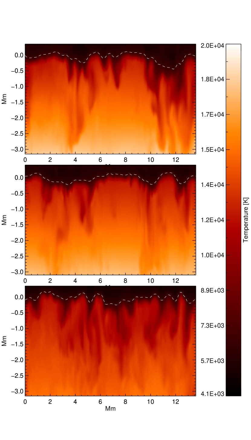
Fig. 5 shows an instantaneous vertical cross-section in the $y$-$z$ plane of temperature from simulations A, B and E. The cooler coherent vertical structures (shaded) extending from the surface of the star to lower heights are called plumes. They are generated by radiative cooling at the photosphere. As the rotation is increased the vertical extent of the plumes reduces. The effect is visible in the figure, where plumes in the non-rotating simulation (top panel) extend down to at least -3Mm below the surface, while for the rotating cases (lower panels), they only reach a depth of about -2Mm. The vertical correlation or mixing length are significantly reduced by rotation.

Figure 5: Snapshots of the upper part of a vertical cross-section of temperature field for $\Omega^{*}=0$ (upper panel), 0.064 (middle panel) and 0.128 (lower panel). These are taken from models A, B and E. Dashed lines shows the $T=T_{\rm eff}$ surface across each slice, and depth is measured with respect to the mean $T_{\rm eff}$ surface. The principle effect of rotation is to reduce the penetration depth of the plumes.

3.2.1 Vertical scale of convective eddies

While the visual inspection of instantaneous snapshots is informative, to better understand what is happening in the turbulent flow we need to look at statistics averaged over many turnover times. Although there is no ‘mixing length’ in 3D RHD simulations, there are several ways of measuring an equivalent quantity.

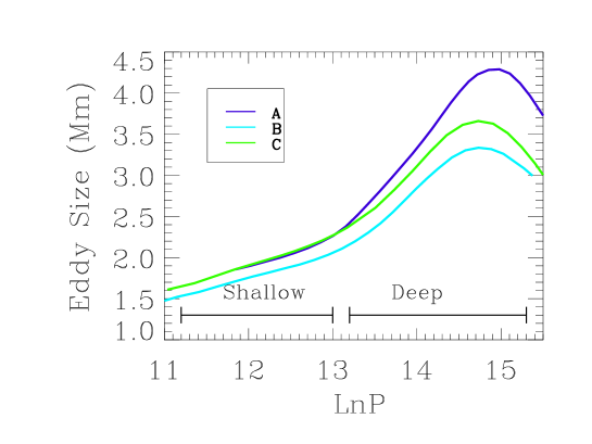
To estimate the length of a characteristic eddy, $l_{z}$, we computed the spatial auto-correlation (equation 4) of the $v_{z}^{\prime}$ field, and define $l_{z}$ as the distance at which $C[v_{z}^{\prime}v_{z}^{\prime}]$ falls to $0.5$. If we assume that the convective eddies have an aspect ratio of unity, then $l_{z}$ gives us an idea of the size of the eddies in a turbulent fluid.

Fig. 6 shows $l_{z}$ for models A, B and C. Comparing Model A and model B, one can see that rotation has much more impact on the eddy size in the lower half of the domain. In the shallow regions, $l_{z}$ is about 10 % smaller for model B compared to model A, whereas in the deep layers, it is about 30% smaller. The effect of rotation on eddy size is three times greater for deep efficient convection, than it is for shallow inefficient convection. The reduction in correlation length with depth is consistent with the decrease in penetration depth of the plumes in the previous figure. In general, the size of the eddies increases, until they are about one scale height from the base. The drop off in eddy size near LnP = 15 is due to the approaching impenetrable bottom surface.

Comparing simulations C and B illustrates the effect of the centrifugal force on the eddy size. These two simulations have the same Coriolis force, but $g$ is 10 % lower in C relative to B to account for the centrifugal force. The reduction in $g$ between C and B, results in an increase of $l_{z}$ of about 10 %. This is because $l_{z}$ is proportional to the local scale height, ${\rm H_{P}}$ which is $\approx{\rm RT}/g$, where R and T are the universal gas constant and temperature, respectively (Robinson et al., 2004; Magic et al., 2015).

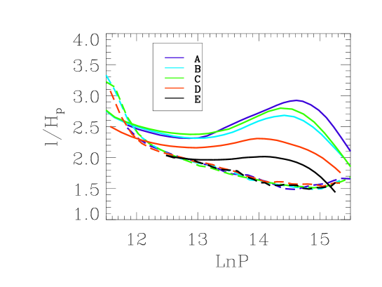
Another convenient measure of the stellar mixing length is the so-called ‘mass-mixing length’, $l_{m}$, described in Trampedach & Stein (2011). Using their equation for $l_{m}$ we computed $l_{m}$ for the upflows as,

$$l_{m}(z)=\Bigl{|}{\frac{{\rm dln}\overline{\rho}}{\rm{dz}}+\frac{{\rm dln}\overline{v_{z}}}{\rm{dz}}+\frac{{\rm dln}\overline{A}}{\rm{dz}}}\Bigr{|}^{-1}$$ (6)

where A is the horizontal area occupied by upflows and overbars denote horizontal and time averages. Fig. 7 shows $l_{z}$ (solid lines) and $l_{m}$ (long dashed lines), each divided by ${\rm H_{P}}$, versus depth. While the $l_{z}$ depends on rotation, $l_{m}$ is almost the same for all five simulations. Rotation does not appear to have any impact on the mass mixing length.

Figure 6: Vertical eddy size, $l_{z}$, versus LnP for models A, B and C. Coriolis force does not appear to affect the near-surface eddy sizes, while the centrifugal force reduces the eddy size at all depths. The effect of rotation is more pronounced in the deeper regions of efficient convection.

Figure 7: Mass mixing length ($l=l_{m}$, long dashes) and eddy size ($l=l_{z}$, solid) divided by local pressure scale height. Rotation has a large effect on eddy sizes (especially in the deeper layers), but no effect on mass mixing length.

3.2.2 Kinetic energy flux

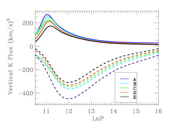
Fig. 8 shows the flux of kinetic energy per unit mass by downdrafts (dashed) and updrafts (solid) for simulations A-E. The quantity plotted is $\overline{v_{z}K}$ where $K=1/2({{v_{x}}^{2}+{v_{y}}^{2}+{v_{z}}^{2}})$. Comparing this plot with the plot of the SAL (Fig 3), one can see that the flux of K by upflows is strongest near the peak of the SAL (LnP = 11) and by downflows is strongest near the base of the SAL (LnP = 12). The flux by the downflows is about double that by the upflows. The effect of rotation on the flux of K is quite significant. The peak downflow and upflow of K drops by roughly 30% between model A and E.

Figure 8: Flux of kinetic energy per unit mass for models A, B, C, D and E. The updrafts and downdrafts are represented by solid and dashed lines, respectively

3.3 Effect of rotation on shallow vs. deep convection

One of the robust features of efficient (deep) convection in $f$-planes at the equator is the linear increase in mean zonal velocity, $\overline{v_{y}}$ with depth. In the study of deep convection by Chan (2001), the slope was shown to be $-2\Omega^{*}$ regardless of input flux or rotation rate. The upper panel of Fig. 9 shows $\overline{v_{y}}$ versus depth for the five models. The closeness of the slope of $\overline{v_{y}}$ to $-2\Omega^{*}$ in the deep layers indicates convergence. There is a clear distinction between deep and shallow convection. In the deep region the slope of $\overline{v_{y}}$ versus depth is constant (and equal to $-2\Omega^{*}$), while in the shallow layers the zonal velocity is approximately constant.

Figure 9: Non-dimensional $\overline{v_{y}}$ (Upper panel) and $\overline{v_{z}}$ (lower panel) versus depth.

In Chan (2001) the $-2\Omega^{*}$ shear was explained by conservation of angular momentum. We will briefly repeat their explanation. To conserve angular momentum, the angular velocity of fluid parcels moving outwards will decrease and that of parcels moving inwards will increase. Consider the effect of only the Coriolis force on a fluid parcel moving upwards or downwards at the equator (where all quantities are in non-dimensional units):

$$\frac{dv_{y}}{dt}\sim-2\Omega v_{z}$$ (7)

$$\frac{\Delta{v_{y}}}{\Delta t}\sim-2\Omega\frac{\Delta{z}}{\Delta t}$$ (8)

$$\frac{\Delta{v_{y}}}{\Delta{z}}\sim-2\Omega$$ (9)

This explains why $v_{y}$ decreases with a slope of -2$\Omega^{*}$ inwards for deep efficient convection. However, for shallow convection, we find that $v_{y}$ is roughly constant, so that

$$\frac{\Delta{v_{y}}}{\Delta{z}}\sim 0$$ (10)

The change in slope signals the transition from shallow inefficient convection (granulation) to deep efficient convection. Without the SAL, the ${\overline{v_{y}}}$ would have a constant -2$\Omega^{*}$ variation with depth throughout the domain.

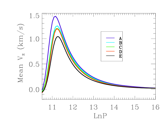
The analysis in section 3.2.1 showed that the eddy size is weakly dependent on rotation in the shallow layers. It is restricted by the granulation. This is why for shallow convection, $l_{z}$ is similar for rotating and non-rotating convection. However, in the deeper layers $l_{z}$ is significantly reduced by rotation. In the deep layers fluid parcels are not controlled by the upflow/downflows associated with the SAL, they are free to feel the full effect of rotation. The lower panel of Fig. 9 shows the mean vertical velocity as a function of depth. When the mean vertical velocity is high, the zonal velocity is constant. When the mean vertical velocity is small (below LnP = 13), the zonal velocity decreases inwards with a slope of -2 $\Omega^{*}$.

3.4 Discussion

Why don’t the fluid parcels in the shallow layers appear to conserve angular momentum as they move radially inwards or outwards? The Coriolis force acts throughout the fluid, but in the shallow regions its effect on the vertically moving fluid parcels is much weaker than it is in the deeper layers. The shallow layers, which are occupied by the granules, move more like a rigid body with little variation with depth. This type of ‘rigid-body rotation’ was suggested by Foukal & Jokipii (1975), as a feature of the near-surface shear layer in the Sun. They estimated that neither the drag produced by viscosity nor the drag from magnetic flux tubes, were large enough to fix the rotation velocity in the upper layers/photosphere, and that some other mechanism was responsible. In the recent simulations of the near surface shear layer by Matilsky et al. (2019), they describe ‘rotationally unconstrained’ fluid as being associated with fast down-flowing plumes. In our simulations, these ‘rotationally unconstrained’ fluid parcels are at the depths occupied by the strongest upflow and downflows.

4 Summary and Conclusions

Rotation is typically ignored in simulations of granulation in the outer layers of stars. This is a reasonable assumption, provided the star does not spin too fast. If it does, then rotation weakens the turbulent vigor, which lowers the superadiabatic layer. In addition, even though rotation is the same throughout the box, its effect is much weaker in the shallow layers compared to the deeper layers. To conserve angular momentum, the angular velocity of the parcel should increase as it moves radially inwards towards the rotation axis (or equivalently to the bottom of the $f$-plane box). However, in our simulations we find that the angular velocity is approximately constant over the first 2 scale heights below layer (SAL) and then linearly increases inwards. Fluid parcels moving towards the rotation axis do not increase their angular velocity until they are below the SAL. We attribute this restriction on angular velocity to the strong vertical motions associated with the SAL. It appears that the short-scale faster overturning motions in the SAL are too quick to be significantly affected by the Coriolis force.

One way to test this hypothesis, is to compare the timescales of fluid parcels in the shallow and deep layers, to the rotation period of the box. A rough estimate for the timescale of an eddy is $\tau_{\rm eddy}=l_{z}/{\overline{v}_{z}}$, where $l_{z}$ is the eddy size and ${\overline{v_{z}}}$ is the mean vertical velocity. Taking values for model B directly from Fig.  6 and the lower panel of Fig.  9, we find that in the shallow region, $l_{z}\sim$ 2000 km and ${\overline{v_{z}}}\sim 1$ km/s, implying $\tau_{\rm eddy}\sim$ 30 minutes, which is 24 times smaller than the 12 hour rotation period. In the deep layers, $l_{z}\sim$ 3000km and ${\overline{v_{z}}}\sim$ 0.1 km/s, implying a timescale of about 8 hours, much closer to the rotation period of the box. These estimates, though crude, support the hypothesis that the external rotation rate of the box will impact fluid parcels in the deeper layers much more than parcels just below the surface of the star. This can also be expressed in terms of a non-dimensional flow parameter called the Coriolis number (or inverse Rossby number), Co =$\Omega\tau_{\rm eddy}$. Rotational effects are less prominent in the surface layers because Co is much smaller there. The variation of ${\overline{v_{y}}}$ with Co for a much larger range of Co values, is described in Chan (2003)

Results that may be of interest to stellar modellers, are the effect of rotation on the SAL, the turbulent pressure and the invariance of the mass mixing length to rotation. The impact of rotation on convection near the top of the star could affect the macro and micro turbulence parameters computed from 3D simulations (Steffen et al., 2009), and particularly in hot stars, such as F stars with ultra thin convection zones, the change in macroturbulence could impact the interpretation of stellar spectra (Saar & Osten, 1997). These results are also relevant to convection in the outer layers of young active stars which rotate much more rapidly (Brown et al., 2008).

The results described in this paper apply to realistic surface convection at the equator. We have not yet examined different latitudes nor examined the effect of a spherical shell geometry — since the $f$-plane box has periodic boundary conditions, it is unable to produce a realistic meridional circulation. However, out aim was to study the effect of rotation on convection, and not large scale flows, and our results show that there are measurable effects which can impact stellar structure,

5 Appendix: Compressibility

As the time step in the numerical schemes is limited by the time for a sound wave to cross between two grid points (known as the C.F.L. condition), to reach a steady state, requires a huge number of timesteps. To ease this restriction, many of the global models use “sound proof” equations such as the Boussinesq (Spiegel & Veronis, 1960) or anelastic (Gough, 1969) approximations, in modelling solar differential rotation (Miesch et al., 2006; Featherstone & Miesch, 2015). By comparing the momentum equation for the Boussinesq, anelastic and fully compressible models, one can see how baroclinicity is modelled in each system. Excluding rotation and viscosity (to simplify the analysis), the momentum equation can be written as

$$\rho\frac{D{\bf v}}{Dt}=-\nabla p^{\prime}-g\rho^{\prime}{\bf e_{k}}$$ (11)

where $p^{\prime}$ and $\rho^{\prime}$ are the perturbation pressure and density (i.e. the hydrostatic part has been removed), and the material derivative is

$$\frac{D}{Dt}=\frac{\partial}{\partial t}+({\bf v}\cdot\nabla).$$ (12)

Depending on the particular choice of $\rho$ in the inertia term one obtains,

1. the incompressible Boussinesq model: $\rho=\rho_{\rm o}$ : constant reference state

2. the anelastic model: $\rho=\rho_{\rm o}(r)$ : spherically symmetric reference state

3. the fully compressible model: $\rho=\rho(r,\theta,\phi,t)$ : full baroclinicity

For the anelastic approximation

$$\nabla\times\frac{\nabla p^{\prime}}{\rho_{\rm o}(r)}=(0,{\omega_{\theta}}^{*},{\omega_{\phi}}^{*})$$ (13)

where ${\omega_{i}}^{*}$ is related to vorticity production. In the anelastic model there is zero contribution to radial vorticity production from the pressure gradient term. It is unclear whether solar differential rotation is being driven primarily from above or below the convection zone. If it is being driven by surface cooling, as suggested by Cossette & Rast (2016) and Käpylä et al. (2017), then it might require a fully compressible model to reproduce features such as the near surface shear layer.

References

- Abbett et al. (1997) Abbett W. P., Beaver M., Davids B., Georgobiani D., Rathbun P., Stein R. F., 1997, The Astrophysical Journal, 480, 395
- Beeck et al. (2012) Beeck B., et al., 2012, Astronomy & Astrophysics, 539, A121
- Böhm-Vitense (1958) Böhm-Vitense E., 1958, Zeitschrift fur Astrophysik, 46, 108
- Brandenburg et al. (2005) Brandenburg A., Chan K., Nordlund A., Stein R., 2005, Astronomische Nachrichten: Astronomical Notes, 326, 681
- Brown et al. (2008) Brown B. P., Browning M. K., Brun A. S., Miesch M. S., Toomre J., 2008, The Astrophysical Journal, 689, 1354
- Brummell et al. (1996) Brummell N. H., Hurlburt N. E., Toomre J., 1996, The Astrophysical Journal, 473, 494
- Brun & Toomre (2002) Brun A. S., Toomre J., 2002, The Astrophysical Journal, 570, 865
- Brun et al. (2011) Brun A. S., Miesch M. S., Toomre J., 2011, The Astrophysical Journal, 742, 79
- Brun et al. (2017) Brun A. S., et al., 2017, The Astrophysical Journal, 836, 192
- Chan (2001) Chan K. L., 2001, The Astrophysical Journal, 548, 1102
- Chan (2003) Chan K. L., 2003, in 3D Stellar Evolution. p. 168
- Chan (2007) Chan K., 2007, Astronomische Nachrichten: Astronomical Notes, 328, 1059
- Chan & Mayr (2013) Chan K. L., Mayr H. G., 2013, Earth and Planetary Science Letters, 371, 212
- Chan & Sofia (1989) Chan K. L., Sofia S., 1989, ApJ, 336, 1022
- Chiavassa et al. (2018) Chiavassa A., Casagrande L., Collet R., Magic Z., Bigot L., Thévenin F., Asplund M., 2018, Astronomy & Astrophysics, 611, A11
- Collet et al. (2007) Collet R., Asplund M., Trampedach R., 2007, Astronomy & Astrophysics, 469, 687
- Cossette & Rast (2016) Cossette J.-F., Rast M. P., 2016, The Astrophysical Journal Letters, 829, L17
- Demarque et al. (2008) Demarque P., Guenther D., Li L., Mazumdar A., Straka C., 2008, Astrophysics and Space Science, 316, 31
- Featherstone & Miesch (2015) Featherstone N. A., Miesch M. S., 2015, The Astrophysical Journal, 804, 67
- Foukal & Jokipii (1975) Foukal P., Jokipii J., 1975, The Astrophysical Journal, 199, L71
- Freytag & Steffen (2004) Freytag B., Steffen M., 2004, in Zverko J., Ziznovsky J., Adelman S. J., Weiss W. W., eds, IAU Symposium Vol. 224, The A-Star Puzzle. pp 139–147, doi:10.1017/S174392130400448X
- Freytag et al. (2002) Freytag B., Steffen M., Dorch B., 2002, Astronomische Nachrichten, 323, 213
- Freytag et al. (2012) Freytag B., Steffen M., Ludwig H.-G., Wedemeyer-Böhm S., Schaffenberger W., Steiner O., 2012, Journal of Computational Physics, 231, 919
- Gough (1969) Gough D., 1969, Journal of the atmospheric sciences, 26, 448
- Hotta et al. (2014) Hotta H., Rempel M., Yokoyama T., 2014, The Astrophysical Journal, 798, 51
- Käpylä et al. (2010) Käpylä P. J., Korpi M. J., Brandenburg A., Mitra D., Tavakol R., 2010, Astronomische Nachrichten: Astronomical Notes, 331, 73
- Käpylä et al. (2017) Käpylä P. J., Rheinhardt M., Brandenburg A., Arlt R., Käpylä M. J., Lagg A., Olspert N., Warnecke J., 2017, The Astrophysical Journal Letters, 845, L23
- Kim & Chan (1998) Kim Y.-C., Chan K. L., 1998, The Astrophysical Journal Letters, 496, L121
- Kim et al. (1996) Kim Y.-C., Fox P. A., Demarque P., Sofia S., 1996, The Astrophysical Journal, 461, 499
- Kitiashvili et al. (2016) Kitiashvili I. N., Kosovichev A. G., Mansour N. N., Wray A. A., 2016, The Astrophysical Journal Letters, 821, L17
- Kupka (2008) Kupka F., 2008, in , Interdisciplinary Aspects of Turbulence. Springer, pp 1–57
- Kupka et al. (2005) Kupka F., Alecian G., Richard O., Vauclair S., 2005
- Ludwig et al. (2002) Ludwig H.-G., Allard F., Hauschildt P. H., 2002, Astronomy & Astrophysics, 395, 99
- Magic et al. (2013a) Magic Z., Collet R., Asplund M., Trampedach R., Hayek W., Chiavassa A., Stein R., Nordlund Å., 2013a, Astronomy & Astrophysics, 557, A26
- Magic et al. (2013b) Magic Z., Collet R., Asplund M., Trampedach R., Hayek W., Chiavassa A., Stein R. F., Nordlund Å., 2013b, A&A, 557, A26
- Magic et al. (2013c) Magic Z., Collet R., Hayek W., Asplund M., 2013c, Astronomy & Astrophysics, 560, A8
- Magic et al. (2015) Magic Z., Weiss A., Asplund M., 2015, Astronomy & Astrophysics, 573, A89
- Mathur et al. (2011) Mathur S., et al., 2011, The Astrophysical Journal, 741, 119
- Matilsky et al. (2019) Matilsky L. I., Hindman B. W., Toomre J., 2019, The Astrophysical Journal, 871, 217
- Miesch (2007) Miesch M., 2007, Astronomische Nachrichten: Astronomical Notes, 328, 998
- Miesch & Hindman (2011) Miesch M. S., Hindman B. W., 2011, The Astrophysical Journal, 743, 79
- Miesch et al. (2006) Miesch M. S., Brun A. S., Toomre J., 2006, The Astrophysical Journal, 641, 618
- Molenda-Zakowicz et al. (2009) Molenda-Zakowicz J., Frasca A., Latham D., 2009, arXiv preprint arXiv:0907.0816
- Mosumgaard et al. (2018) Mosumgaard J. R., Ball W. H., Silva Aguirre V., Weiss A., Christensen-Dalsgaard J., 2018, Monthly Notices of the Royal Astronomical Society, 478, 5650
- Nelson et al. (2018) Nelson N. J., Featherstone N. A., Miesch M. S., Toomre J., 2018, The Astrophysical Journal, 859, 117
- Nordlund (1985) Nordlund A., 1985, Sol. Phys., 100, 209
- Nordlund & Galsgaard (1995) Nordlund Å., Galsgaard K., 1995, A 3D MHD code for Parallel Computers
- Palacios & Brun (2007) Palacios A., Brun A., 2007, Astronomische Nachrichten: Astronomical Notes, 328, 1114
- Pedlosky & Robertson (1988) Pedlosky J., Robertson J., 1988, Geophysical fluid dynamics by Joseph Pedlosky
- Robinson & Chan (2001) Robinson F. J., Chan K. L., 2001, Monthly Notices of the Royal Astronomical Society, 321, 723
- Robinson et al. (2003) Robinson F., Demarque P., Li L. H., Sofia S., Kim Y.-C., Chan K., Guenther D., 2003, Monthly Notices of the Royal Astronomical Society, 340, 923
- Robinson et al. (2004) Robinson F., Demarque P., Li L., Sofia S., Kim Y.-C., Chan K., Guenther D., 2004, Monthly Notices of the Royal Astronomical Society, 347, 1208
- Robinson et al. (2005) Robinson F. J., Demarque P., Guenther D., Kim Y.-C., Chan K., 2005, Monthly Notices of the Royal Astronomical Society, 362, 1031
- Rutten et al. (1995) Rutten R. J., et al., 1995, Radiative transfer in stellar atmospheres. Sterrekundig Instituut Utrecht
- Saar & Osten (1997) Saar S., Osten R., 1997, Monthly Notices of the Royal Astronomical Society, 284, 803
- Smagorinsky (1963) Smagorinsky J., 1963, Monthly weather review, 91, 99
- Solano & Fernley (1997) Solano E., Fernley J., 1997, Astronomy and Astrophysics Supplement Series, 122, 131
- Spada et al. (2018) Spada F., Demarque P., Basu S., Tanner J., 2018, The Astrophysical Journal, 869, 135
- Spiegel & Veronis (1960) Spiegel E. A., Veronis G., 1960, The Astrophysical Journal, 131, 442
- Steffen et al. (2009) Steffen M., Ludwig H.-G., Caffau E., 2009, arXiv preprint arXiv:0909.2831
- Stein & Nordlund (2000) Stein R. F., Nordlund Å., 2000, pp 91–108
- Tanner et al. (2012) Tanner J. D., Basu S., Demarque P., 2012, The Astrophysical Journal, 759, 120
- Tanner et al. (2013) Tanner J. D., Basu S., Demarque P., 2013, The Astrophysical Journal, 767, 78
- Tanner et al. (2016) Tanner J. D., Basu S., Demarque P., 2016, The Astrophysical Journal Letters, 822, L17
- Trampedach & Stein (2011) Trampedach R., Stein R. F., 2011, The Astrophysical Journal, 731, 78
- Trampedach et al. (2013a) Trampedach R., Asplund M., Collet R., Nordlund Å., Stein R. F., 2013a, The Astrophysical Journal, 769, 18
- Trampedach et al. (2013b) Trampedach R., Asplund M., Collet R., Nordlund Å., Stein R. F., 2013b, The Astrophysical Journal, 769, 18
- Unno & Spiegel (1966) Unno W., Spiegel E., 1966, Publications of the Astronomical Society of Japan, 18, 85
- Vögler et al. (2005) Vögler A., Shelyag S., Schüssler M., Cattaneo F., Emonet T., Linde T., 2005, Astronomy & Astrophysics, 429, 335
- Wedemeyer et al. (2013) Wedemeyer S., Ludwig H.-G., Steiner O., 2013, Astronomische Nachrichten, 334, 137