Robust Exact Differentiators with Predefined Convergence Time

Abstract

The problem of exactly differentiating a signal with bounded second derivative is considered. A class of differentiators is proposed, which converge to the derivative of such a signal within a fixed, i.e., a finite and uniformly bounded convergence time. A tuning procedure is derived that allows to assign an arbitrary, predefined upper bound for this convergence time. It is furthermore shown that this bound can be made arbitrarily tight by appropriate tuning. The usefulness of the procedure is demonstrated by applying it to the well-known uniform robust exact differentiator, which is included in the considered class of differentiators as a special case.

, , , ,

1 Introduction

The real-time computation of the exact derivative of a measured signal is a very important problem that has many useful applications, such as robust state estimation and fault detection. A variety of successful approaches to real-time signal differentiation is based on homogeneous sliding-mode algorithms, see, e.g. (Levant, 1998, 2003; Levant et al., 2017). Due to homogeneity, these approaches have several useful features: robustness with respect to measurement noise, convergence to the derivative in finite time, and existence of appropriate discrete-time implementations (Livne and Levant, 2014; Koch and Reichhartinger, 2019; Koch et al., 2020).

Among these features, finite-time convergence (see Roxin, 1966; Bhat and Bernstein, 2000) is one of the most important advantages because, in theory, it allows to exactly reconstruct states and even perturbations within a finite time (Floquet and Barbot, 2007; Bejarano et al., 2007; Li et al., 2014). In a control context, this advantage permits to separate design and stability analysis of the differentiator (i.e., the observer) from that of a nonlinear state-feedback controller. This separation becomes possible because the controller can be switched on after the differentiator has converged (Angulo et al., 2013a). In practice, an upper bound for the finite convergence time is required. While such a bound always exists, it may grow infinitely large with increasingly large initial conditions. To overcome this disadvantage, a stronger stability notion was introduced by Cruz-Zavala et al. (2011) (see also Angulo et al., 2013b) that is uniform with respect to the initial condition and was later called fixed-time convergence (Polyakov, 2011; Polyakov and Fridman, 2014). This property guarantees that the convergence time is uniformly upper bounded by a fixed finite time irrespective of the initial condition. While fixed-time convergent differentiators are not homogeneous, they are typically designed to retain most of the corresponding useful features.

One of the most successful approaches for differentiation in finite time is the first-order robust exact differentiator (Levant, 1998). This differentiator is based on the so-called super-twisting algorithm (STA) originally proposed by Levant (1993), and can differentiate signals with Lipschitz continuous time derivative. Higher-order derivatives can be obtained using its arbitrary-order generalization (Levant, 2003) or also by cascading first-order differentiators in a step-by-step manner (Floquet and Barbot, 2007; Bejarano et al., 2007).

Several extensions of STA-based differentiators with fixed-time convergence exist. Examples are the uniformly convergent arbitrary order differentiator (Angulo et al., 2013b) and the first-order uniform robust exact differentiator proposed by Cruz-Zavala et al. (2011). For the latter, a generalization was presented by Moreno (2011) in the form of the generic second order algorithm, which itself is further generalized as the disturbance-tailored STA by Haimovich and De Battista (2019).

An important practical problem is how to make the convergence time satisfy a desired global upper bound. Together with state-feedback control, this allows the designer to tune beforehand also the time after which the controller is turned on. For the uniform robust exact differentiator, this problem is studied empirically in Fraguela et al. (2012). More recently, the related concepts of prescribed-time stability by Holloway and Krstic (2019) and predefined-time stability by Sánchez-Torres et al. (2015, 2017) have been proposed in that regard. The former concept studies ways to prescribe the actual convergence time, rather than its upper bounds, typically by employing time-varying gains that tend to infinity at the desired convergence time instant (Holloway and Krstic, 2019) or by varying the homogeneity degree (Chitour et al., 2020). The latter concept studies systems for which an arbitrary convergence time bound can be specified by a suitable choice of some free parameters (Sánchez-Torres et al., 2015) or by means of a time-varying redesign of given fixed-time stable systems (Gómez-Gutiérrez, 2020). Algorithms studied in that regard typically are focused on closed loops obtained from controllers, however, rather than differentiators.

Causing a sliding-mode differentiator to satisfy a prescribed convergence time is a challenging problem that requires reasonably tight convergence time bounds. For fixed-time differentiators based on the STA, convergence time bounds were obtained in the course of a Lyapunov-based stability analysis (see, e.g. Moreno, 2011). Simple convergence time bounds for another differentiator approach are given by Basin (2019) (see also references therein). This approach, however, is suitable only for functions with constant time derivative, as shown by Seeber (2020b). For the STA, i.e., the first-order robust exact differentiator, convergence time bounds have been studied more extensively, see, e.g., the recent tutorial (Seeber, 2020a) and references therein. Notably, asymptotically exact bounds have been obtained in Seeber et al. (2018) by computing the STA’s convergence time in the form of an improper integral.

The present paper proposes a new class of first-order fixed-time convergent differentiators along with a tuning paradigm for assigning an upper bound to its global uniform convergence time. The considered differentiator is based on the disturbance-tailored STA from Haimovich and De Battista (2019), and thus includes the uniform robust exact differentiator as a special case. The differentiator’s convergence time is studied by extending the convergence time computation and the corresponding asymptotically exact bounds from Seeber et al. (2018). The tuning paradigm is obtained by combining these bounds with a homogeneity-like scaling property of the global convergence time.

The paper is structured as follows. Section 2 states the considered problem of obtaining a signal’s time derivative within a given finite time, and Section 3 discusses the differentiator structure used for this purpose and its properties. Section 4 proposes a tuning procedure to solve the problem. The main theorem—Theorem 4.8—permits to specify a bound for the differentiator’s convergence time based on the computation of only a single convergence time bound for an arbitrary parameter setting. After illustrating the proposed tuning procedure in Section 5 by means of examples, Sections 6 and 7 compute the convergence time function and study the global convergence time of the proposed differentiator, thereby providing the tools required for the presented tuning paradigm. Conclusions are given in Section 8. Section 9 forms an appendix that provides proofs for the technical lemmas used in the paper.

Notation: ${\mathbb{R}}$, ${\mathbb{R}}_{\geq 0}$, ${\mathbb{R}}_{>0}$ denote the reals, nonnegative reals, and positive reals, respectively. If $\alpha\in{\mathbb{R}}$, then $|\alpha|$ denotes its absolute value. For $x\in{\mathbb{R}}^{n}$, $\left\|x\right\|$ denotes its Euclidean norm. For $y,p\in{\mathbb{R}}$, the abbreviations $\left\lfloor y\right\rceil^{p}=\left|y\right|^{p}\,\mathrm{sign}(y)$ and $\left\lfloor y\right\rceil^{0}=\,\mathrm{sign}(y)$ are used. The symbol ‘$\,{\scriptstyle\circ}\,$’ denotes function composition. If $\nu:D\subseteq{\mathbb{R}}\to{\mathbb{R}}$, then $\nu^{\prime}$ denotes the derivative of $\nu$. A superscript ^T denotes matrix or vector transposition. For a function $\gamma:{\mathbb{R}}_{>0}\to{\mathbb{R}}$, define $\gamma(0):=\lim_{s\to 0^{+}}\gamma(s)$ provided the limit exists. Furthermore, $\gamma^{-1}$ denotes the inverse function, if it exists, and $\gamma^{\prime}$ is written for the derivative of the function with respect to its argument, unless it is a function of time, in which case $\dot{\gamma}$ denotes its time derivative. The convention $\inf A=\infty$ is used if $A$ is the empty set. $\lambda_{\min}(\cdot)$ and $\lambda_{\max}(\cdot)$ denote the minimum and maximum eigenvalues, respectively, of a symmetric matrix, and $\operatorname{diag}(d_{1},\ldots,d_{n})\in{\mathbb{R}}^{n\times n}$ denotes a diagonal matrix with diagonal entries $d_{1},\ldots,d_{n}$.

2 Problem Statement

Let $f:{\mathbb{R}}_{\geq 0}\to{\mathbb{R}}$ be a continuously differentiable function, whose time derivative $\dot{f}$ is globally Lipschitz continuous, i.e., whose second time derivative $\ddot{f}$ for almost all $t$ satisfies

$$\left|\ddot{f}(t)\right|\leq L$$ (1)

with a nonnegative Lipschitz constant $L$. The goal is to exactly reconstruct the time derivative $\dot{f}$ within a desired, fixed time $T>0$, i.e., to obtain $\dot{f}(t)$ for $t\geq T$ from $f(t)$ for $t\geq 0$. Thus, the following problem is addressed.

Problem 1.

Given a Lipschitz constant $L\geq 0$ and a time $T>0$, construct a dynamic system—a differentiator—that takes a function $f$ as input and generates an output $y$ satisfying $y(t)=\dot{f}(t)$ for all $t\geq T$, for every function $f$ satisfying (1).

3 Differentiator Structure

Problem 1 will be solved employing a differentiator having the structure

$$\dot{y}_{1} =k_{1}\nu_{1}(f-y_{1})+y_{2}$$ (2a)

$$\dot{y}_{2} =k_{2}\nu_{2}(f-y_{1})$$ (2b)

$$y =y_{2}$$ (2c)

with state variables $y_{1},y_{2}$, functions $\nu_{1},\nu_{2}:{\mathbb{R}}\to{\mathbb{R}}$ given by

$$\nu_{1}(x) =k_{3}^{-1}\Phi(k_{3}^{2}x), \nu_{2}(x) =2\Phi(k_{3}^{2}x)\Phi^{\prime}(k_{3}^{2}x),$$ (3)

and parameters $k_{1},k_{2},k_{3}>0$. The function $\Phi:{\mathbb{R}}\to{\mathbb{R}}$ is called the Differentiator Generating Function (DGF) and is defined next. Afterwards, the convergence time function of the differentiator and its uniform upper bound, the global convergence time, are introduced. The differentiator’s asymptotic robustness properties are also discussed.

3.1 Differentiator Generating Function

The DGF $\Phi$ has to satisfy the following definition.

Definition 1 (Differentiator Generating Function).

A locally absolutely continuous function $\Phi:{\mathbb{R}}\to{\mathbb{R}}$ is called a Differentiator Generating Function (DGF) if it has the following properties:

1. $\Phi$ is odd, i.e., $\Phi(-x)=-\Phi(x)$ for all $x\in{\mathbb{R}}$,

2. $\Phi$ and $\Phi^{\prime}$ are continuously differentiable in ${\mathbb{R}}\setminus\{0\}$,

3. $\Phi^{\prime}$ is positive, i.e., $\Phi^{\prime}(x)>0$ for all $x\in{\mathbb{R}}\setminus\{0\}$,

4. $\lim_{x\to 0}|\Phi^{\prime}(x)|=\infty$,

5. $\lim_{x\to 0}\left|\frac{2\Phi^{\prime}(x)^{3}}{\Phi^{\prime\prime}(x)}\right|=1$.

According to conditions (i) and (ii), $\nu_{1}$ and $\nu_{2}$ both are odd functions that are continuous and locally Lipschitz in ${\mathbb{R}}\setminus\{0\}$. The remaining conditions—in particular the limits—yield the following properties of the functions $\nu_{1}$ and $\nu_{2}$, which are formally proven in Section 9.

Lemma 3.1.

Consider a DGF $\Phi$ and let $k_{3}>0$. Then, the functions $\nu_{1},\nu_{2}$ defined in (3) satisfy

$$\lim_{\alpha\to 0}\frac{\nu_{1}(\alpha^{2}x)^{2}}{\alpha^{2}}=\left|x\right|,\qquad\lim_{\alpha\to 0}\left|\nu_{2}(\alpha^{2}x)\right|=1$$ (4)

uniformly in $x$ on every compact subset of ${\mathbb{R}}\setminus\{0\}$.

As a consequence of (4), and since the function $\nu_{2}$ is odd, it is discontinuous in the origin. Hence, the right-hand side of (2b) is discontinuous, and solutions of (2) are understood in the sense of Filippov (1988). When $y_{1}=f$, specifically, (2b) is to be read as the differential inclusion

$$\dot{y}_{2}\in\bigl{[}-k_{2}\lim_{x\to 0^{+}}\nu_{2}(x),-k_{2}\lim_{x\to 0^{-}}\nu_{2}(x)\bigr{]}=[-k_{2},k_{2}].$$ (5)

From this relation, one can see that $L\leq k_{2}$ is a necessary condition for the differentiator to converge, because maintaining $y_{2}(t)=\dot{f}(t)$ requires $|\ddot{f}(t)|\leq k_{2}$.

Remark 3.2.

Functions that satisfy the conditions of Definition 1 are $\Phi(x)=\left\lfloor x\right\rceil^{\frac{1}{2}}$ and $\Phi(x)=\left\lfloor x\right\rceil^{\frac{1}{2}}+\left\lfloor x\right\rceil^{\frac{3}{2}}$, for example. These yield the robust exact differentiator proposed in Levant (1998) and the uniform robust exact differentiator proposed in Cruz-Zavala et al. (2011), respectively.

By means of the selected structure, the more specific problem that will be solved can now be stated.

Problem 2.

Given $L\geq 0$ and $T>0$, select a suitable DGF $\Phi$ and positive design parameters $k_{1},k_{2},k_{3}$ such that solutions of (2) satisfy $y(t)=\dot{f}(t)$ for all $t\geq T$, for every function $f$ satisfying (1) and every initial condition $y_{1}(0),y_{2}(0)\in{\mathbb{R}}$.

3.2 Differentiator Error and Convergence Time

To study the differentiator’s convergence behavior, the error variables $x_{1}:=f-y_{1}$, $x_{2}:=\dot{f}-y_{2}$ are introduced and aggregated in the vector $\bm{x}=[x_{1}\quad x_{2}]^{\mathrm{T}}$ in the following. For notational convenience, the family of functions $\Phi_{\epsilon}:{\mathbb{R}}\to{\mathbb{R}}$ is furthermore defined as

$$\Phi_{\epsilon}(x)=\epsilon^{-1}\Phi(\epsilon^{2}x),$$ (6)

which satisfies $\Phi^{\prime}_{\epsilon}(x)=\epsilon\Phi(\epsilon^{2}x)$. Using this notation, one has $\nu_{1}=\Phi_{k_{3}}$ and $\nu_{2}=2\Phi_{k_{3}}\Phi_{k_{3}}^{\prime}$. The corresponding error dynamics then are

$$\dot{x}_{1} =-k_{1}\nu_{1}(x_{1})+x_{2}=-k_{1}\Phi_{k_{3}}(x_{1})+x_{2}$$ (7a)

$$\dot{x}_{2} =-k_{2}\nu_{2}(x_{1})+\ddot{f}=-2k_{2}\Phi_{k_{3}}(x_{1})\Phi_{k_{3}}^{\prime}(x_{1})+\ddot{f}$$ (7b)

with

$$\left|\ddot{f}\right|\leq L.$$ (7c)

One can see that $\ddot{f}$ enters this system as a perturbation. The case $\ddot{f}=0$, i.e., $L=0$, is hence called unperturbed case in the following, while $L\geq 0$ is referred to as perturbed case.

If $\Phi$ satisfies Definition 1, then (7) is a well-defined Filippov inclusion, whose solutions exist and are continuable in forward time. Let $\bm{x}(\cdot,\bm{x}_{0},f)$ denote the solution to (7) satisfying $\bm{x}(0,\bm{x}_{0},f)=\bm{x}_{0}$. Let $\tau(\bm{x}_{0},f)$ denote the minimum time $t$ that the trajectory $\bm{x}(\cdot,\bm{x}_{0},f)$ takes to converge to the origin, i.e.,

$$\tau(\bm{x}_{0},f) =\inf\{t\geq 0:\bm{x}(\sigma,\bm{x}_{0},f)=0\quad\forall\sigma\geq t\}.$$ (8)

Depending on the DGF $\Phi$, the parameters

$$\bm{k}:=(k_{1},k_{2},k_{3}),$$ (9)

the initial state $\bm{x}_{0}$ and the function $f$, the convergence time $\tau(\bm{x}_{0},f)$ may be finite or infinite.

The worst-case convergence time obtained for any $f$ satisfying (1) as a function of the initial state $\bm{x}_{0}$ is called the convergence time function of system (7). It is denoted by $T^{\Phi,\bm{k}}_{L}:{\mathbb{R}}^{2}\to{\mathbb{R}}$ and is given by

$$T^{\Phi,\bm{k}}_{L}(\bm{x}_{0}):=\sup_{\left|\ddot{f}\right|\leq L}\tau(\bm{x}_{0},f).$$ (10)

The smallest uniform upper bound of this function with respect to the initial state

$$\hat{\mathbb{T}}(\Phi,\bm{k},L):=\sup_{\bm{x}_{0}\in{\mathbb{R}}^{2}}T^{\Phi,\bm{k}}_{L}(\bm{x}_{0})$$ (11)

is called the differentiator’s global convergence time. Using this notation, Problem 2 may be restated as follows.

Problem 2 (restated).

Given $L\geq 0$ and $T>0$, select a suitable DGF $\Phi$ and positive design parameters $k_{1},k_{2},k_{3}$ so that the differentiator’s global convergence time satisfies $\hat{\mathbb{T}}(\Phi,\bm{k},L)\leq T$.

Note that, depending on $\Phi$ and $\bm{k}$, the global convergence time may be finite or infinite even when the convergence time function yields finite values for all initial states. Fixed-time convergence refers to the case of finite $\hat{\mathbb{T}}(\Phi,\bm{k},L)$, whereas (global) finite-time convergence just indicates that $T^{\Phi,\bm{k}}_{L}(\bm{x}_{0})$ is finite for every $\bm{x}_{0}\in{\mathbb{R}}^{2}$ but does not guarantee that $\hat{\mathbb{T}}(\Phi,\bm{k},L)$ is also finite. For these cases, Lyapunov stability of the origin will additionally be shown, which guarantees that solutions of (7) are also unique in forward time.

3.3 Asymptotic Properties and Robustness

Homogeneously approximating the inclusion (7) at the origin in the sense of (Andrieu et al., 2008, Definition 2.1) with degree $-1$ and weights $(2,1)$ yields the super-twisting algorithm, i.e., the first-order robust exact differentiator:

Theorem 3.3 (Asymptotic Behavior).

For every DGF $\Phi$ and every $k_{3}>0$, the STA system

$$\dot{x}_{1}=-k_{1}\left\lfloor x_{1}\right\rceil^{\frac{1}{2}}+x_{2},\qquad\dot{x}_{2}=-k_{2}\left\lfloor x_{1}\right\rceil^{0}+\ddot{f}$$ (12)

is a homogeneous approximation of (7) at the origin.

Remark 3.4.

As a consequence of this theorem, asymptotic (small-signal) measurement noise gains and robustness properties of the proposed differentiator are the same as for the first-order robust exact differentiator, see Levant (1998), provided that $k_{1},k_{2}$ are chosen such that (7) and (12) both converge in finite time for all $\ddot{f}$ satisfying (7c).

Using the limits (4) and symmetry properties of $\nu_{1},\nu_{2}$ defined in (3), one obtains from (7)

$$\lim_{\alpha\to 0}\frac{-k_{1}\nu_{1}(\alpha^{2}x_{1})+\alpha x_{2}}{\alpha} =-k_{1}\left\lfloor x_{1}\right\rceil^{\frac{1}{2}}+x_{2},$$

$$\lim_{\alpha\to 0}\bigl{(}-k_{2}\nu_{2}(\alpha^{2}x_{1})+\ddot{f}\bigr{)} =-k_{2}\left\lfloor x_{1}\right\rceil^{0}+\ddot{f}.$$

Due to Lemma 3.1, the limits are uniform in $x_{1},x_{2}$ on compact sets; hence, (12) is a homogeneous approximation of (7) according to (Andrieu et al., 2008, Definition 2.1). $\hfill\blacksquare$

4 Design Procedure

This section provides a solution to Problem 2. First, requirements on the DGF $\Phi$ are formulated, which provide a guideline for its design. Then, a tuning procedure for the parameters $k_{1},k_{2},k_{3}$ is proposed, which is based on a single upper bound of the global convergence time for one set of parameter values. Thus, a complete design procedure is developed.

4.1 Design of the Differentiator Generating Function

Selecting a DGF according to Definition 1 provides for a well-posed Filippov inclusion and will be shown in Section 6 to yield a finite convergence time $T_{0}^{\Phi,\bm{k}}(\bm{x}_{0})$ for $L=0$. This does not guarantee, however, that the global convergence time $\hat{\mathbb{T}}(\Phi,\bm{k},L)$ is finite, especially for $L>0$. In the following, conditions on the DGF are therefore formulated that will allow to establish a finite global convergence time bound. They are motivated by the following result, which is proven in Section 7.2.

Proposition 4.1.

Let $\bm{k}=(k_{1},k_{2},k_{3})\in{\mathbb{R}}_{>0}^{3}$, $L\in{\mathbb{R}}_{\geq 0}$ and consider a DGF $\Phi$. If $k_{1}^{2}\geq 8k_{2}$, then

$$\hat{\mathbb{T}}(\Phi,\bm{k},L)\geq\frac{2}{\bigl{(}k_{1}-\sqrt{k_{1}^{2}-8k_{2}}\bigr{)}k_{3}}\int_{0}^{\infty}\frac{1}{\Phi(x)}\,\mathrm{d}x.$$ (13)

One can see that under the conditions of this proposition, the DGF $\Phi$ has to be selected such that the integral on the right-hand side of (13) exists and is finite. The concept of an admissible DGF is thus introduced, which satisfies this condition along with some additional technical assumptions.

Definition 2 (Admissibility of DGFs).

A DGF $\Phi$ is called admissible if there exist constants $B>0$, $C>0$, and $D\geq 1$ such that $\Phi$ satisfies

1. $\int_{0}^{\infty}\frac{1}{B\Phi(x)}\,\mathrm{d}x\leq 1$,

2. $C\Phi^{\prime}(x)\geq 1$ for all $x\in{\mathbb{R}}\setminus\{0\}$,

3. $2D|\Phi^{\prime}(x)|^{3}\geq|\Phi^{\prime\prime}(x)|$ for all $x\in{\mathbb{R}}\setminus\{0\}$.

Condition (i) is required for fixed-time convergence, i.e., for the global convergence time to be finite. The other two conditions (ii) and (iii) can be interpreted as a uniform variant of item (iii) and a global variant of item (v) of Definition 1, respectively. They will be used to establish a convergence time bound when $L>0$. In particular, condition (ii) guarantees that $\Phi(x)$ grows without bound as $x\to\infty$; and condition (iii) implies the existence of a uniform lower bound for $\left|2\Phi_{k_{3}}(x)\Phi_{k_{3}}^{\prime}(x)\right|$, because it is equivalent to

$$\frac{\mathrm{d}{\Phi(x)}}{\mathrm{d}{x}}\geq\frac{1}{2D}\frac{\mathrm{d}{}}{\mathrm{d}{x}}\frac{1}{\Phi^{\prime}(x)},$$ (14)

i.e., $\Phi$ grows faster than $\Phi^{\prime}$ decays. Such a lower bound is necessary for finite-time stability with $L>0$, because otherwise system (7) exhibits an additional non-zero equilibrium for any arbitrarily small (and constant) $\ddot{f}$.

Remark 4.2.

Both $\Phi(x)=\left\lfloor x\right\rceil^{\frac{1}{2}}$ and $\Phi(x)=\left\lfloor x\right\rceil^{\frac{1}{2}}+\left\lfloor x\right\rceil^{\frac{3}{2}}$ satisfy item (iii) of Definition 2 with $D=1$. Only the latter is actually admissible, however, due to item (i).

Remark 4.3.

Note that in the context of the disturbance-tailored super-twisting (DTST) algorithm proposed by Haimovich and De Battista (2019), the pair $(\nu_{1},\nu_{2})$ defined in (3) is DTST-admissible when $\Phi$ is an admissible DGF.

4.2 Tuning of the Differentiator’s Parameters

The proposed tuning procedure, i.e., the procedure for selecting appropriate values for the differentiator’s parameters $k_{1},k_{2},k_{3}$, is based on the following proposition, which in part has also been noted empirically by Fraguela et al. (2012). A formal proof is provided in Section 7.1.

Proposition 4.4 (Scaling of Parameters).

Let $\bm{k}\in{\mathbb{R}}_{>0}^{3}$, $L\geq 0$ and consider a DGF $\Phi$. Then, the global worst-case convergence time (11) of system (7) satisfies

$$\hat{\mathbb{T}}\Bigl{(}\Phi,\bm{D}_{\alpha,\beta}\bm{k},\alpha^{2}L\Bigr{)}=\frac{1}{\alpha\beta}\hat{\mathbb{T}}\Bigl{(}\Phi,\bm{k},L\Bigr{)}.$$ (15)

with $\bm{D}_{\alpha,\beta}=\operatorname{diag}(\alpha,\alpha^{2},\beta)$ for all $\alpha,\beta\in{\mathbb{R}}_{>0}$.

Proposition 4.4 shows how the global convergence time depends on specific scalings of the parameters $\bm{k}$ and the Lipschitz constant $L$. The following result allows, in addition, to bound the worst-case convergence time corresponding to a positive $L$ in terms of that corresponding to $L=0$. Its proof is also given in Section 7.1.

Proposition 4.5 (Variation of Lipschitz Constant).

Let $L\geq 0$, $\bm{k}=(k_{1},k_{2},k_{3})\in{\mathbb{R}}^{3}_{>0}$, consider an admissible DGF $\Phi$ with $D\geq 1$ as in Definition 2 and define

$$\overline{L}=\begin{cases}\frac{k_{2}}{D}&\text{if }k_{1}^{2}\geq 8k_{2}\\ \frac{k_{2}}{D}\tanh\dfrac{\pi k_{1}}{2\sqrt{8k_{2}-k_{1}^{2}}}&\text{if }k_{1}^{2}<8k_{2}.\end{cases}$$ (16)

If $L<\overline{L}$, then

$$\hat{\mathbb{T}}(\Phi,\bm{k},L)\leq\frac{\hat{\mathbb{T}}(\Phi,\bm{k},0)}{1-L\overline{L}^{-1}}.$$ (17)

Remark 4.6.

Note that $k_{2}>LD$ is necessary for the conditions of Proposition 4.5 to be satisfied, while $k_{2}>L$ is a necessary condition for the finite-time stability of (7). Thus, it is desirable to keep $D\geq 1$ as small as possible when designing or choosing an admissible DGF $\Phi$.

In order to simplify tuning, the following notion of a normalized parameter triple is introduced.

Definition 3 (Normalized Parameter Triple).

A parameter triple $\bm{k}=(k_{1},k_{2},k_{3})\in{\mathbb{R}}_{>0}^{3}$ is called normalized with respect to an admissible DGF $\Phi$, if there exists a $D$ satisfying Definition 2, i.e.,

$$D\geq\sup_{x\in{\mathbb{R}}}\frac{\left|\Phi^{\prime\prime}(x)\right|}{2\left|\Phi^{\prime}(x)\right|^{3}},$$ (18)

such that $\overline{L}\geq 1$ in (16).

Since $\overline{L}$ can be interpreted as an upper bound for the Lipschitz constant $L$, a normalized parameter triple ensures that fixed-time convergence can be guaranteed for all $L\leq 1$.

Proposition 4.5 shows that it is sufficient to consider the case $L=0$ when studying upper bounds for the global convergence time. As the final prerequisite for the proposed tuning procedure, the following proposition gives such a bound. It is proven in Section 7.3.

Proposition 4.7 (Global Convergence Time Bound).

Let $\bm{k}=(k_{1},k_{2},k_{3})\in{\mathbb{R}}_{>0}^{3}$ and consider an admissible DGF $\Phi$ with $B,C\in{\mathbb{R}}_{>0}$ as in Definition 2. If $k_{1}^{2}\geq 8k_{2}$, then $\hat{\mathbb{T}}(\Phi,\bm{k},0)\leq\tilde{T}(\Phi,\bm{k})$ with

$$\tilde{T}(\Phi,\bm{k})=\begin{cases}\frac{\ln\frac{k_{1}+\sqrt{k_{1}^{2}-8k_{2}}}{k_{1}-\sqrt{k_{1}^{2}-8k_{2}}}}{2k_{3}\sqrt{k_{1}^{2}-8k_{2}}}\scriptstyle C+\frac{k_{1}^{2}+4k_{2}}{2k_{1}k_{2}k_{3}}B,&k_{1}^{2}>8k_{2},\\ \vspace{5pt}\cr\frac{C+6B}{k_{1}k_{3}},&k_{1}^{2}=8k_{2}.\end{cases}$$ (19)

By combining Propositions 4.4 and 4.5, the scalar parameters $k_{1},k_{2},k_{3}$ may be computed from a single, arbitrary convergence time bound obtained using Proposition 4.7. This is stated as the following theorem.

Theorem 4.8 (Tuning).

Let a Lipschitz constant $L\geq 0$ and a desired convergence time $T>0$ be given. Consider an admissible DGF $\Phi$, let $\tilde{\bm{k}}=(\tilde{k}_{1},\tilde{k}_{2},\tilde{k}_{3})\in{\mathbb{R}}_{>0}^{3}$ be a normalized parameter triple with respect to $\Phi$, and suppose that

$$\hat{\mathbb{T}}(\Phi,\tilde{\bm{k}},0)\leq\tilde{T}$$ (20)

holds for some $\tilde{T}>0$. Define $\bm{k}=(k_{1},k_{2},k_{3})$ via

$$k_{1} =\tilde{k}_{1}\sqrt{\gamma}, k_{2} =\tilde{k}_{2}\gamma, k_{3} =\frac{\tilde{k}_{3}\sqrt{\gamma}}{\gamma-L}\cdot\frac{\tilde{T}}{T}$$ (21)

for some $\gamma>L$. Then, the global convergence time of the differentiator (2) satisfies the bound

$$\hat{\mathbb{T}}(\Phi,\bm{k},L)\leq T.$$ (22)

Remark 4.9.

Note that $\gamma$ acts as a tradeoff parameter that determines the relative magnitude of the parameters $k_{1},k_{2},k_{3}$ without influencing the convergence time. With increasing $\gamma$, the parameter $k_{3}$ decreases, while the parameters $k_{1},k_{2}$, which according to Theorem 3.3 determine the behavior of system (7) close to the origin, increase.

Remark 4.10.

Table 1 lists normalized parameter tuples for two admissible DGFs, along with the bound $\tilde{T}$ in (20) that may be used for differentiator tuning with this theorem. The table’s contents are derived in Section 5.

According to Proposition 4.4

$$\hat{\mathbb{T}}(\Phi,\bm{k},L)=\frac{\gamma-L}{\gamma}\frac{T}{\tilde{T}}\hat{\mathbb{T}}(\Phi,\tilde{\bm{k}},\gamma^{-1}L).$$ (23)

Furthermore, since $\tilde{\bm{k}}$ is normalized, Proposition 4.5 may be applied with $\overline{L}\geq 1$ to obtain

$$\hat{\mathbb{T}}(\Phi,\tilde{\bm{k}},\gamma^{-1}L)\leq\frac{1}{1-\gamma^{-1}L\overline{L}^{-1}}\hat{\mathbb{T}}(\Phi,\tilde{\bm{k}},0)\leq\frac{\gamma}{\gamma-L}\tilde{T}.$$ (24)

Combining the two relations completes the proof. $\hfill\blacksquare$

	$\sqrt{8}$	$5$	$10$	$15$	$20$
$\left\lfloor x\right\rceil^{\frac{1}{2}}+\left\lfloor x\right\rceil^{\frac{3}{2}}$	$6.9$	$9.3$	$16.5$	$24.1$	$31.9$
$\sqrt{\mathrm{e}^{\left|x\right|}-1}\left\lfloor x\right\rceil^{0}$	$7.1$	$9.4$	$16.6$	$24.2$	$31.9$

Table 1: Gain $\tilde{k}_{1}$ and corresponding bound $\tilde{T}$, computed using (20), of normalized parameter triples with $\tilde{k}_{2}=\tilde{k}_{3}=1$ for two admissible DGFs, to be used for differentiator tuning with Theorem 4.8

4.3 Tightness of Predefined Convergence Time

By using the lower bound for $\hat{\mathbb{T}}(\Phi,\bm{k},L)$ from Proposition 4.1, the conservatism of the predefined convergence time may be bounded from above, provided that the value of the improper integral in Definition 2 is known exactly:

Theorem 4.11 (Tightness of Assigned Bound).

Let $T>0$ and $\gamma>L\geq 0$, consider an admissible DGF $\Phi$, and suppose that $B$ is such that equality holds in item (i) of Definition 2. Suppose that $\tilde{k}_{1}$, $\tilde{k}_{2}$, $\tilde{k}_{3}$, and $\tilde{T}$ satisfy the conditions of Theorem 4.8 and that $\tilde{k}_{1}^{2}\geq 8\tilde{k}_{2}$. If parameters $k_{1},k_{2},k_{3}$ are selected using (21), then the ratio of predefined and actual global convergence time is bounded from above by

$$\frac{T}{\hat{\mathbb{T}}(\Phi,\bm{k},L)}\leq\frac{\Bigl{(}\tilde{k}_{1}-\sqrt{\tilde{k}_{1}^{2}-8\tilde{k}_{2}}\Bigr{)}\tilde{k}_{3}\tilde{T}}{2B}\cdot\frac{\gamma}{\gamma-L}.$$ (25)

Moreover, if $\tilde{T}=\tilde{T}(\Phi,\tilde{\bm{k}})$ from (19), then this upper bound tends to $\frac{\gamma}{\gamma-L}$ for $\tilde{k}_{1}\to\infty$.

Remark 4.12.

As a consequence, provided that $B$ is tight and (19) is used, the assigned convergence time bound can be made arbitrarily tight by increasing $\tilde{k}_{1}$ and $\gamma$.

Abbreviate $\tilde{h}=\sqrt{\tilde{k}_{1}^{2}-8\tilde{k}_{2}}$ for convenience. Rewriting $T$ in (21), one has

$$T=\frac{\tilde{k}_{3}\tilde{T}\sqrt{\gamma}}{(\gamma-L)k_{3}}.$$ (26)

Definition 2, item (i) and Proposition 4.1 furthermore yield

$$\hat{\mathbb{T}}(\Phi,\bm{k},L)\geq\frac{2B}{\Bigl{(}k_{1}-\sqrt{k_{1}^{2}-8k_{2}}\Bigr{)}k_{3}}=\frac{2B}{\Bigl{(}\tilde{k}_{1}-\tilde{h}\Bigr{)}\sqrt{\gamma}k_{3}}.$$ (27)

Dividing the two expressions yields the bound (25). Now, substitute $\tilde{q}_{1}=\tilde{k}_{2}\tilde{k}_{1}^{-2}$ and $\tilde{q}_{2}=(\tilde{k}_{1}+\tilde{h})(\tilde{k}_{1}-\tilde{h})^{-1}$ in the multipliers of $B$ and $C$ in the expression $(\tilde{k}_{1}-\tilde{h})\tilde{k}_{3}\tilde{T}(\Phi,\tilde{\bm{k}})$, and apply L’Hôpital’s rule for $\tilde{q}_{1}\to 0$ and $\tilde{q}_{2}\to\infty$ to show that they tend to two and zero, respectively, as $\tilde{k}_{1}\to\infty$. $\hfill\blacksquare$

5 Design Examples

5.1 Uniform Robust Exact Differentiator

As an application of the proposed tuning procedure, consider the uniform robust exact differentiator (Cruz-Zavala et al., 2011). It is generated by the DGF $\Phi(x)=\left\lfloor x\right\rceil^{\frac{1}{2}}+\left\lfloor x\right\rceil^{\frac{3}{2}}$ and is obtained from (2) and (3) as

$$\dot{y}_{1} =k_{1}(\left\lfloor f-y_{1}\right\rceil^{\frac{1}{2}}+k_{3}^{2}\left\lfloor f-y_{1}\right\rceil^{\frac{3}{2}})+y_{2}$$ (28a)

$$\dot{y}_{2} =k_{2}(\left\lfloor f-y_{1}\right\rceil^{0}+4k_{3}^{2}(f-y_{1})+3k_{3}^{4}\left\lfloor f-y_{1}\right\rceil^{2}).$$ (28b)

This DGF is admissible with

$$B =\int_{0}^{\infty}\frac{1}{\Phi(x)}\mathrm{d}x=\int_{0}^{\infty}\frac{\mathrm{d}x}{x^{\frac{1}{2}}+x^{\frac{3}{2}}}=\pi,$$ (29a)

$$C =\sup_{x\in{\mathbb{R}}}\frac{1}{\Phi^{\prime}(x)}=\sup_{x>0}\frac{1}{\frac{1}{2}x^{-\frac{1}{2}}+\frac{3}{2}x^{\frac{1}{2}}}=\frac{1}{\sqrt{3}},$$ (29b)

$$D =\sup_{x\in{\mathbb{R}}}\frac{\left|\Phi^{\prime\prime}(x)\right|}{2\left|\Phi^{\prime}(x)\right|^{3}}=\sup_{x>0}\frac{\left|1-3x\right|}{\left|1+3x\right|^{3}}=1.$$ (29c)

Using (29) and Proposition 4.7, one obtains the normalized parameter triples and associated convergence time bounds in the first row of Table 1. Choosing for example the first of these entries, a predefined convergence time $T$ may be assigned to the uniform robust exact differentiator by selecting $k_{1},k_{2},k_{3}$ according to Theorem 4.8 as

$$k_{1}=\sqrt{8\gamma},\qquad k_{2}=\gamma,\qquad k_{3}=\frac{6.9\sqrt{\gamma}}{(\gamma-L)T}.$$ (30)

Fig. 1 shows simulation results obtained by applying (28) with initial values $y_{1}(0)=y_{2}(0)=0$ to the signal

$$f(t)=0.75\cos(t)+0.0025\sin(10t)+t$$ (31)

with $L=1$ and desired convergence time bound $T=1$. The parameters are chosen according to (30) with $\gamma=4.5L$ as $k_{1}=6$, $k_{2}=4.5$, and $k_{3}\approx 4.182$. For simplicity, the simulation is performed using forward Euler discretization using a sufficiently small step size $T_{\mathrm{s}}=10^{-4}$. Note, however, that such a simple discretization scheme in general does not achieve global stability, as shown by Levant (2013). In practice, more advanced schemes as proposed by Wetzlinger et al. (2019) (cf. also Rüdiger-Wetzlinger et al. (2021)), for example, should therefore be employed.

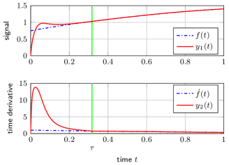
Figure 1: Differentiation of $f(t)=0.75\cos(t)+0.0025\sin(10t)+t$ with $L=1$ and desired convergence time bound $T=1$ by using the proposed differentiator with parameters $k_{1}=6$, $k_{2}=4.5$, $k_{3}\approx 4.182$, initial values $y_{1}(0)=y_{2}(0)=0$, and DGF $\Phi(x)=\left\lfloor x\right\rceil^{1/2}+\left\lfloor x\right\rceil^{3/2}$, along with the actual convergence time $\tau\approx 0.32$, obtained using forward Euler discretization with discretization step size $T_{\mathrm{s}}=10^{-4}$.

Since $B$ is computed in (29a) by solving the integral exactly, Theorem 4.11 may be applied to show that the assigned bound exceeds the worst-case convergence time by no more than a factor of four; this can also be seen in the simulation.

Fig. 2 compares the steady-state differentiation error magnitude achieved using the proposed approach to the robust exact differentiator (i.e., the STA) using the same simulation settings with additional, uniformly bounded measurement noise. As noise, a uniform random number independently sampled with step size $T_{\mathrm{s}}$ is used. For small noise, the behaviors coincide, as shown in Theorem 3.3, and for vanishing noise they are determined by the discretization. Only for very large noises, performance of the fixed-time differentiator eventually deteriorates due to the effectively larger gain that is necessary for achieving fixed-time convergence.

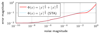
Figure 2: Comparison of steady-state differentiation error magnitude $\sup_{t\in[2,4]}\left|x_{2}(t)\right|$ for the simulation shown in Fig. 1 to the STA (i.e., the robust exact differentiator), with additional, uniformly bounded random measurement noise.

5.2 Exponential Differentiator Generating Function

As another example, consider the DGF

$$\Phi(x)=\sqrt{\exp(\left|x\right|)-1}\left\lfloor x\right\rceil^{0},$$ (32)

which generates the differentiator

$$\dot{y}_{1} =\frac{k_{1}}{k_{3}}\sqrt{\exp(k_{3}^{2}\left|f-y_{1}\right|)-1}\left\lfloor f-y_{1}\right\rceil^{0}+y_{2}$$ (33a)

$$\dot{y}_{2} =k_{2}\exp(k_{3}^{2}\left|f-y_{1}\right|)\left\lfloor f-y_{1}\right\rceil^{0}.$$ (33b)

For this DGF, (tight) admissibility constants are obtained as

$$B =\int_{0}^{\infty}\frac{1}{\Phi(x)}\mathrm{d}x=\int_{0}^{\infty}\frac{\mathrm{d}x}{\sqrt{\mathrm{e}^{x}-1}}=\pi,$$ (34a)

$$C =\sup_{x\in{\mathbb{R}}}\frac{1}{\Phi^{\prime}(x)}=\sup_{x>0}\frac{2\sqrt{\mathrm{e}^{x}-1}}{\mathrm{e}^{x}}=1,$$ (34b)

$$D =\sup_{x\in{\mathbb{R}}}\frac{\left|\Phi^{\prime\prime}(x)\right|}{2\left|\Phi^{\prime}(x)\right|^{3}}=\sup_{x>0}\frac{\left|2\mathrm{e}^{x}-3\right|}{\mathrm{e}^{2x}}=1.$$ (34c)

Using these constants and Proposition 4.7, the second row of Table 1 is obtained.

Fig. 3 depicts convergence times obtained from a simulation for both DGFs when differentiating functions $f(t)$ with different slope and sinusoidal frequency. Simulation settings and parameters were selected as before, but with re-tuned parameter $k_{3}\approx 4.303$ for the exponential DGF to maintain $T=1$ as a global convergence time bound. The variation of the initial slope corresponds to a variation of the error system’s initial condition $x_{2}(0)=\dot{f}(0)$, while $x_{1}(0)=0$. One can see that the convergence time remains bounded by $T$ for all considered functions.

6 Convergence Time Function

This section studies the convergence time of system (7) as a function of the initial state. First, this function is derived for the unperturbed case and for any DGF (even non-admissible ones) in the form of a convergent improper integral. For admissible DGFs, a convergence time bound for the perturbed case is then shown.

Throughout this section as well as the next section, the following abbreviations are used. Given parameters $\bm{k}=(k_{1},k_{2},k_{3})$, define the matrix $\bm{A}\in{\mathbb{R}}^{2\times 2}$, vectors $\bm{e}_{1},\bm{e}_{2}\in{\mathbb{R}}^{2}$, and functions $\bm{g}:{\mathbb{R}}^{2}\to{\mathbb{R}}^{2}$ and $\Psi:{\mathbb{R}}\to{\mathbb{R}}$ as

$$\bm{A} =\begin{bmatrix}-\frac{k_{1}}{2}&\frac{1}{2}\\ -k_{2}&\ 0\end{bmatrix}, \bm{e}_{1} =\begin{bmatrix}1\\ 0\end{bmatrix}, \bm{e}_{2} =\begin{bmatrix}0\\ 1\end{bmatrix},$$ (35a)

$$\bm{g}(\bm{x}) =\begin{bmatrix}\Phi_{k_{3}}(x_{1})\\ x_{2}\end{bmatrix}, \Psi( z)=\Phi_{k_{3}}^{-1}(z),$$ (35b)

wherein according to (6), $\Phi_{\epsilon}^{-1}(z)=\epsilon^{-2}\Phi^{-1}(\epsilon z)$.

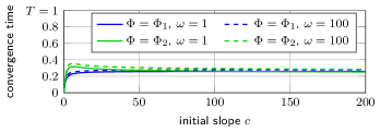
Figure 3: Simulated convergence times obtained by differentiating $f(t)=(\cos\omega t-1)/\omega^{2}+ct$ with settings as in Fig. 1 and two different DGFs $\Phi_{1}(x)=\left\lfloor x\right\rceil^{\frac{1}{2}}+\left\lfloor x\right\rceil^{\frac{3}{2}}$ and $\Phi_{2}(x)=\sqrt{\mathrm{e}^{\left|x\right|}-1}\left\lfloor x\right\rceil^{0}$, both tuned according to Theorem 4.8 with convergence time bound $T=1$ and $\gamma=4.5$, as a function of the initial slope $c=\dot{f}(0)$.

Some basic properties of the function $\Psi$ are first shown in the following technical lemma, which is proven in Section 9.

Lemma 6.1.

Consider a DGF $\Phi$ let $k_{3}\in{\mathbb{R}}_{>0}$. Then, for every $\epsilon>0$ there exist constants $C,D\in{\mathbb{R}}_{>0}$ such that $\Psi$ as defined in (35) satisfies for all $z\in[-\epsilon,\epsilon]$ the inequalities

$$|\Psi^{\prime}(z)|\leq Ck_{3}^{-1},\qquad|\Psi^{\prime\prime}(z)|\leq 2D.$$ (36)

Moreover, if $\Phi$ is an admissible DGF, then (36) holds for all $z$ with $C,D$ as in Definition 2.

6.1 Computation for the Unperturbed Case

Consider system (7) without perturbation, i.e., with $\ddot{f}=0$. It is first shown that the corresponding convergence time function may be represented as an improper integral, which is finite for all positive parameters $\bm{k}$ and all DGFs $\Phi$ that satisfy Definition 1.

Following the ideas presented in Cruz-Zavala et al. (2011), system (7) with $\ddot{f}=0$ and $\bm{z}=\bm{g}(\bm{x})$ may be written as

$$\dot{\bm{z}}=\frac{2}{\Psi^{\prime}(z_{1})}\bm{A}\bm{z}.$$ (37)

As pointed out in Seeber et al. (2018), a linear system $\frac{\mathrm{d}{\bm{z}}}{\mathrm{d}{\tau}}=\bm{A}\bm{z}$ is obtained with respect to a new time variable $\tau$ satisfying $\Psi^{\prime}(z_{1})\mathrm{d}\tau=2\mathrm{d}t$ (this time-scaling idea was employed for the STA for the first time in Moreno and Guzman, 2011). Therefore, one may intuitively expect to obtain the convergence time by integrating $\mathrm{d}t$ along the trajectories of this linear system.

The following technical result, which is proven in Section 9, suggests that this is indeed the case.

Lemma 6.2.

Let $\bm{k}=(k_{1},k_{2},k_{3})\in{\mathbb{R}}_{>0}^{3}$, and consider a DGF $\Phi$. Then, the function $V:{\mathbb{R}}^{2}\to{\mathbb{R}}_{\geq 0}$ given by

$$V(\bm{x})=\int_{0}^{\infty}\frac{1}{2}\Psi^{\prime}(\bm{e}_{1}^{\mathrm{T}}\mathrm{e}^{\bm{A}\tau}\bm{g}(\bm{x}))\,\mathrm{d}\tau$$ (38)

is locally bounded, continuous, and positive definite. For $x_{1}\neq 0$, it is furthermore differentiable and its time derivative $\dot{V}$ along the trajectories of system (7) is given by

$$\dot{V}(t,\bm{x})=-1+\ddot{f}(t)\int_{0}^{\infty}\frac{1}{2}\Psi^{\prime\prime}(\bm{e}_{1}^{\mathrm{T}}\mathrm{e}^{\bm{A}\tau}\bm{g}(\bm{x}))\bm{e}_{1}^{\mathrm{T}}\mathrm{e}^{\bm{A}\tau}\bm{e}_{2}\,\mathrm{d}\tau.$$

The fact that $\dot{V}$ is equal to minus one for $\ddot{f}=0$ suggests that the function $V$ is the unperturbed system’s convergence time function. Since $V$ is not everywhere differentiable, however, the following technical lemma is required, which is obtained following ideas presented in Seeber et al. (2018); Haimovich and De Battista (2019), and is proven in Section 9.

Lemma 6.3.

Let $\bm{k}\in{\mathbb{R}}_{>0}^{3}$, $L\in{\mathbb{R}}_{\geq 0}$, $c\in{\mathbb{R}}_{>0}$ and consider a DGF $\Phi$. Let $V:{\mathbb{R}}^{2}\to{\mathbb{R}}$ be continuous and positive definite and suppose that the time derivative $\dot{V}$ along the trajectories of system (7) is well-defined and bounded by $\dot{V}(t,\bm{x})\leq-c$ for all $t,\bm{x}$ with $x_{1}\neq 0$. Then, the system’s convergence time $T_{L}^{\Phi,\bm{k}}$ is bounded by

$$T_{L}^{\Phi,\bm{k}}(\bm{x})\leq\frac{V(\bm{x})}{c}$$ (39)

and equality holds if $\dot{V}(t,\bm{x})=-c$ for all $t,\bm{x}$ with $x_{1}\neq 0$.

Using this result, the following proposition may now be proven.

Proposition 6.4 (Unperturbed Convergence Time).

Let $\bm{k}=(k_{1},k_{2},k_{3})\in{\mathbb{R}}_{>0}^{3}$, $\bm{x}_{0}\in{\mathbb{R}}^{2}$ and consider a DGF $\Phi$. Then, the convergence time of system (7) for $L=0$ is finite and is given by

$$T_{0}^{\Phi,\bm{k}}(\bm{x}_{0})=\int_{0}^{\infty}\frac{1}{2}\Psi^{\prime}(\bm{e}_{1}^{\mathrm{T}}\mathrm{e}^{\bm{A}\tau}\bm{g}(\bm{x}_{0}))\,\mathrm{d}\tau.$$ (40)

For $\ddot{f}=0$, the continuous, positive definite function $V$ defined in Lemma 6.2 satisfies $\dot{V}(t,\bm{x})=-1$ for $x_{1}\neq 0$. Lemma 6.3 thus yields $T_{0}^{\Phi,\bm{k}}(\bm{x}_{0})=V(\bm{x}_{0})$. Since this function is locally bounded according to Lemma 6.2, one has $T_{0}^{\Phi,\bm{k}}(\bm{x}_{0})<\infty$. $\hfill\blacksquare$

6.2 Bound for the Perturbed Case

Focusing on admissible DGFs, an upper bound for the convergence time function in the perturbed case is now derived. To that end, the following lemma will be used, which expresses the maximum Lipschitz constant $\overline{L}$ defined in Proposition 4.5 in the form of an improper integral.

Lemma 6.5 (Seeber (2020a, Theorem 3)).

Let $k_{1},k_{2},D\in{\mathbb{R}}_{>0}$. Then, $\overline{L}$ defined in (16) is given by

$$\overline{L}=\frac{1}{D\int_{0}^{\infty}|\bm{e}_{1}^{\mathrm{T}}\mathrm{e}^{\bm{A}\tau}\bm{e}_{2}|\,\mathrm{d}\tau}.$$ (41)

Using the auxiliary lemmas, an upper bound for the convergence time function in the perturbed case is obtained.

Proposition 6.6 (Convergence Time Bound).

Let $L\geq 0$, $\bm{k}=(k_{1},k_{2},k_{3})\in{\mathbb{R}}^{3}_{>0}$, consider an admissible DGF $\Phi$, and define $\overline{L}$ as in (16). If $L<\overline{L}$, then

$$T_{L}^{\Phi,\bm{k}}(\bm{x})\leq\frac{T_{0}^{\Phi,\bm{k}}(\bm{x})}{1-L\overline{L}^{-1}}$$ (42)

holds for all $\bm{x}\in{\mathbb{R}}^{2}$.

Let $V$ be the continuous, positive definite function $V$ defined in Lemma 6.2. For $x_{1}\neq 0$, this function is differentiable and using Lemmas 6.2, 6.1, and 6.5 one finds that its time derivative along the trajectories of system (7) is bounded by

$$\dot{V} =-1+\ddot{f}\int_{0}^{\infty}\frac{1}{2}\Psi^{\prime\prime}(\bm{e}_{1}^{\mathrm{T}}\mathrm{e}^{\bm{A}\tau}\bm{g}(\bm{x}))\bm{e}_{1}^{\mathrm{T}}\mathrm{e}^{\bm{A}\tau}\bm{e}_{2}\,\mathrm{d}\tau$$

$$\leq-1+LD\int_{0}^{\infty}|\bm{e}_{1}^{\mathrm{T}}\mathrm{e}^{\bm{A}\tau}\bm{e}_{2}|\,\mathrm{d}\tau=-1+L\overline{L}^{-1}.$$ (43)

Lemma 6.3 then yields

$$T_{L}^{\Phi,\bm{k}}(\bm{x})\leq\frac{V(\bm{x})}{1-L\overline{L}^{-1}}$$ (44)

and using Proposition 6.4 to see that $V(\bm{x})=T_{0}^{\Phi,\bm{k}}(\bm{x})$ concludes the proof. $\hfill\blacksquare$

7 Global Convergence Time

This section investigates properties and bounds of the convergence time function’s smallest upper bound: the global convergence time

$$\hat{\mathbb{T}}(\Phi,\bm{k},L)=\sup_{\bm{x}\in{\mathbb{R}}^{2}}T_{L}^{\Phi,\bm{k}}(\bm{x}).$$ (45)

First, two scaling properties are shown. Then, lower and upper bounds are derived. As before, the quantities introduced in (35) are used throughout this section.

7.1 Scaling Properties

In the following, the scaling properties in Propositions 4.4 and 4.5 are shown. The former utilizes a homogeneity-like scaling property of state, time, and parameters of system (7). The latter is an immediate consequence of Proposition 6.6.

PROOF of Proposition 4.4

Let $x_{1},x_{2}:{\mathbb{R}}_{\geq 0}\to{\mathbb{R}}$ be any solution of (7) with $|\ddot{f}|\leq L$ and denote their convergence time by $\tau$. Consider functions $z_{1},z_{2}:{\mathbb{R}}_{\geq 0}\to{\mathbb{R}}$ given by

$$z_{1}(t)=\beta^{-2}x_{1}(\alpha\beta t),\qquad z_{2}(t)=\alpha\beta^{-1}x_{2}(\alpha\beta t).$$ (46)

Clearly, these converge to zero in time $\tilde{\tau}=\alpha^{-1}\beta^{-1}\tau$ and satisfy

$$\dot{z}_{1} =\alpha\beta^{-1}\dot{x}_{1}=-\alpha k_{1}\beta^{-1}\Phi_{k_{3}}(x_{1})+\alpha\beta^{-1}x_{2}$$

$$=-\alpha k_{1}\beta^{-1}\Phi_{k_{3}}(\beta^{2}z_{1})+z_{2}$$

$$=-\alpha k_{1}\Phi_{\beta k_{3}}(z_{1})+z_{2}$$ (47)

$$\dot{z}_{2} =\alpha^{2}\dot{x}_{2}=-2\alpha^{2}k_{2}\Phi_{k_{3}}(x_{1})\Phi_{k_{3}}^{\prime}(x_{1})+\alpha^{2}\ddot{f}$$

$$=-2\alpha^{2}k_{2}\Phi_{k_{3}}(\beta^{2}z_{1})\Phi_{k_{3}}^{\prime}(\beta^{2}z_{1})+\alpha^{2}\ddot{f}$$

$$=-2\alpha^{2}k_{2}\Phi_{\beta k_{3}}(z_{1})\Phi_{\beta k_{3}}^{\prime}(z_{1})+\alpha^{2}\ddot{f},$$ (48)

i.e., differential equations (7) with parameters $\alpha k_{1}$, $\alpha^{2}k_{2}$, $\beta k_{3}$ and Lipschitz constant $\alpha^{2}L$. $\hfill\blacksquare$

PROOF of Proposition 4.5

Taking the supremum with respect to $\bm{x}$ on each side of (42) yields

$$\hat{\mathbb{T}}(\Phi,\bm{k},L) =\sup_{\bm{x}\in{\mathbb{R}}^{2}}T_{L}^{\Phi,\bm{k}}(\bm{x})$$

$$\leq\sup_{\bm{x}\in{\mathbb{R}}^{2}}\frac{T_{0}^{\Phi,\bm{k}}(\bm{x})}{1-L\overline{L}^{-1}}=\frac{\hat{\mathbb{T}}(\Phi,\bm{k},0)}{1-L\overline{L}^{-1}},$$ (49)

i.e., relation (17), which proves the proposition. $\hfill\blacksquare$

7.2 Lower Bound

Explicitly solving the integral in (40) is not possible in general. An interesting special case is obtained if $\bm{g}(\bm{x})$ is an eigenvector of $\bm{A}$ with eigenvalue $\lambda$. In this case, one has

$$\bm{e}_{1}^{\mathrm{T}}\mathrm{e}^{\bm{A}\tau}\bm{g}(\bm{x})=c\mathrm{e}^{\lambda\tau}$$ (50)

with some $c\in{\mathbb{R}}$. As the following lemma shows, the integral in (40) may then be simplified further. Its proof is given in Section 9.

Lemma 7.1.

Let $k_{3}\in{\mathbb{R}}_{>0}$, $\lambda\in{\mathbb{R}}_{<0}$, $c\in{\mathbb{R}}$ and consider a DGF $\Phi$. Then,

$$\int_{0}^{\infty}\Psi^{\prime}(c\mathrm{e}^{\lambda\tau})\,\mathrm{d}\tau=-\frac{1}{k_{3}\lambda}\int_{0}^{\Phi^{-1}(k_{3}c)}\frac{1}{\Phi(x)}\,\mathrm{d}x.$$ (51)

It should be highlighted that the use of this lemma does not require the knowledge of the DGF’s inverse $\Phi^{-1}$. Proposition 4.1, which provided the original motivation for the definition of an admissible DGF, may now be proven.

PROOF of Proposition 4.1

Since $k_{1}^{2}\geq 8k_{2}$, the matrix $\bm{A}$ has real eigenvalues and its largest eigenvalue is given by

$$\lambda=\frac{-k_{1}+\sqrt{k_{1}^{2}-8k_{2}}}{4}.$$ (52)

Denote by $\mathcal{D}$ the set of all $\bm{x}\in{\mathbb{R}}^{2}$ such that $\bm{g}(\bm{x})$ is an eigenvector of $\bm{A}$ with this eigenvalue. Using Proposition 6.4 and Lemma 7.1, one then has

$$\hat{\mathbb{T}}(\Phi,\bm{k},L) \geq\sup_{\bm{x}\in\mathcal{D}}T_{0}^{\Phi,\bm{k}}(\bm{x})=\sup_{c\in{\mathbb{R}}}\int_{0}^{\infty}\frac{1}{2}\Psi^{\prime}(c\mathrm{e}^{\lambda\tau})\,\mathrm{d}\tau$$

$$=\sup_{c\in{\mathbb{R}}}-\frac{1}{2k_{3}\lambda}\int_{0}^{\Phi^{-1}(k_{3}c)}\frac{1}{\Phi(x)}\,\mathrm{d}x$$

$$=\frac{2\int_{0}^{\infty}\frac{1}{\Phi(x)}\,\mathrm{d}x}{\bigl{(}k_{1}-\sqrt{k_{1}^{2}-8k_{2}}\bigr{)}k_{3}}.$$ (53)

This concludes the proof.$\hfill\blacksquare$

7.3 Upper Bound

Upper bounds for the global convergence time are now studied. According to the results in the previous sections, it is sufficient to consider such bounds for $L=0$, since bounds for $L>0$ can then be obtained using Proposition 4.5. Using Proposition 6.4, the expression to bound from above is given by

$$\hat{\mathbb{T}}(\Phi,\bm{k},0)=\sup_{\bm{z}\in{\mathbb{R}}^{2}}\int_{0}^{\infty}\frac{1}{2}\Psi^{\prime}(\bm{e}_{1}^{\mathrm{T}}\mathrm{e}^{\bm{A}\tau}\bm{z})\,\mathrm{d}\tau.$$ (54)

As a first step towards finding the supremum, the following lemma, which is proven in Section 9, is given. It allows to restrict the range of $\bm{z}$ to a compact subset of ${\mathbb{R}}^{2}$ by extending the domain of integration. In case the eigenvalues of $\bm{A}$ are real-valued and distinct, the integrand may furthermore be simplified.

Lemma 7.2.

Consider an admissible DGF $\Phi$, define the compact set $\mathcal{D}=\{\bm{v}\in{\mathbb{R}}^{2}:\left\|\bm{v}\right\|=1\}$, and let $\bm{k}=(k_{1},k_{2},k_{3})\in{\mathbb{R}}_{>0}^{3}$. Then,

$$\hat{\mathbb{T}}(\Phi,\bm{k},0)=\sup_{\bm{v}\in\mathcal{D}}\int_{-\infty}^{\infty}\frac{1}{2}\Psi^{\prime}(\bm{e}_{1}^{\mathrm{T}}\mathrm{e}^{\bm{A}\tau}\bm{v})\,\mathrm{d}\tau.$$ (55)

Furthermore, if $k_{1}^{2}>8k_{2}$, then

$$\hat{\mathbb{T}}(\Phi,\bm{k},0)=\sup_{a\in{\mathbb{R}}}\int_{-\infty}^{\infty}\frac{1}{2}\Psi^{\prime}(|a|\mathrm{e}^{\lambda_{1}\tau}+a\mathrm{e}^{\lambda_{2}\tau})\,\mathrm{d}\tau$$ (56)

holds with the eigenvalues $\lambda_{1},\lambda_{2}\in{\mathbb{R}}_{<0}$

$$\lambda_{1}=-\frac{k_{1}-\sqrt{k_{1}^{2}-8k_{2}}}{4},\quad\lambda_{2}=-\frac{k_{1}+\sqrt{k_{1}^{2}-8k_{2}}}{4}$$ (57)

of the matrix $\bm{A}$.

In order to obtain global bounds, the following lemma is used, which is essentially an extension of Lemma 7.1 and is proven in Section 9.

Lemma 7.3.

Let $k_{3}>0$ and consider an admissible DGF $\Phi$ and a (possibly unbounded) interval $(a,b)\subseteq{\mathbb{R}}$. Let furthermore $h:(a,b)\to{\mathbb{R}}$ be a continuously differentiable function, which for some $\alpha\in{\mathbb{R}}$ satisfies

$$h^{\prime}(\tau)\geq\alpha h(\tau)>0$$ (58)

for all $\tau\in(a,b)$. Then, with $\Psi$ as defined in (35b), one has

$$\int_{a}^{b}\Psi^{\prime}(h(\tau))\,\mathrm{d}\tau\leq\frac{1}{k_{3}\alpha}\int_{\Phi^{-1}(k_{3}h(a))}^{\Phi^{-1}(k_{3}h(b))}\frac{1}{\Phi(x)}\,\mathrm{d}x.$$ (59)

Using these results, Proposition 4.7 may now be proven.

PROOF of Proposition 4.7:

The second case $k_{1}^{2}=8k_{2}$ in (19) is obtained as the limit of the first case as $k_{1}^{2}$ tends to $8k_{2}$. Hence, it is sufficient to consider the case $k_{1}^{2}>8k_{2}$ in the following. In this case, one has $\hat{\mathbb{T}}(\Phi,\bm{k},0)=\sup_{a\in{\mathbb{R}}}T_{a}$ according to Lemma 7.2 with

$$T_{a}=\int_{-\infty}^{\infty}\frac{1}{2}\Psi^{\prime}(|a|\mathrm{e}^{\lambda_{1}\tau}+a\mathrm{e}^{\lambda_{2}\tau})\,\mathrm{d}\tau$$ (60)

and $\lambda_{2}<\lambda_{1}$ as in (57). Consider first the case $a\geq 0$. Since $\Psi^{\prime}(-z)=\Psi^{\prime}(z)$, one may apply Lemma 7.3 with $h(\tau)=-a\mathrm{e}^{\lambda_{1}\tau}-a\mathrm{e}^{\lambda_{2}\tau}$. This function satisfies $h(\tau)<0$ and

$$h^{\prime}(\tau)=\lambda_{1}h(\tau)+a(\lambda_{1}-\lambda_{2})\mathrm{e}^{\lambda_{2}\tau}\geq\lambda_{1}h(\tau)>0$$ (61)

for all $\tau\in{\mathbb{R}}$, because $\lambda_{2}<\lambda_{1}<0$. One thus obtains

$$T_{a}\leq\frac{\int_{-\infty}^{0}\frac{1}{\Phi(x)}\,\mathrm{d}x}{2k_{3}\lambda_{1}}=-\frac{\int_{0}^{\infty}\frac{1}{\Phi(x)}\,\mathrm{d}x}{2k_{3}\lambda_{1}}\leq-\frac{B}{2k_{3}\lambda_{1}}.$$ (62)

For the case $a<0$, let $b=-a>0$ and consider the function

$$\tilde{h}_{b}(\tau)=|a|\mathrm{e}^{\lambda_{1}\tau}+a\mathrm{e}^{\lambda_{2}\tau}=b(\mathrm{e}^{\lambda_{1}\tau}-\mathrm{e}^{\lambda_{2}\tau}).$$ (63)

On the interval $I_{1}=(-\infty,0)$ this function is strictly increasing and satisfies in particular $\tilde{h}_{b}(\tau)<0$ and

$$\tilde{h}^{\prime}_{b}(\tau)=\lambda_{2}\tilde{h}_{b}(\tau)+b(\lambda_{1}-\lambda_{2})\mathrm{e}^{\lambda_{1}\tau}\geq-\frac{k_{1}}{4}\tilde{h}_{b}(\tau)$$ (64)

for all $\tau\in I_{1}$. It furthermore has a single inflection point

$$\tau_{\mathrm{inf}}=\frac{2}{\lambda_{1}-\lambda_{2}}\ln\frac{\lambda_{2}}{\lambda_{1}}=\frac{\ln\frac{k_{1}+\sqrt{k_{1}^{2}-8k_{2}}}{k_{1}-\sqrt{k_{1}^{2}-8k_{2}}}}{\sqrt{k_{1}^{2}-8k_{2}}},$$ (65)

i.e., $\tilde{h}_{b}^{\prime\prime}(\tau_{\mathrm{inf}})=0$. On the interval $I_{3}=(\tau_{\mathrm{inf}},\infty)$, one has $\tilde{h}_{b}^{\prime\prime}(\tau)>0$; thus

$$(\lambda_{1}+\lambda_{2})\tilde{h}_{b}^{\prime}(\tau)=\lambda_{1}\lambda_{2}\tilde{h}_{b}(\tau)+\tilde{h}_{b}^{\prime\prime}(\tau)>\lambda_{1}\lambda_{2}\tilde{h}_{b}(\tau).$$ (66)

and consequently

$$\tilde{h}_{b}^{\prime}(\tau)\leq\frac{\lambda_{1}\lambda_{2}}{\lambda_{1}+\lambda_{2}}\tilde{h}_{b}(\tau)=-\frac{k_{2}}{k_{1}}\tilde{h}_{b}(\tau)<0$$ (67)

holds for all $\tau\in I_{3}$. Therefore, Lemma 7.3 may be used with $h=\tilde{h}_{b}$ or $h=-\tilde{h}_{b}$ on the intervals $I_{1}$ or $I_{3}$, respectively, to bound the integral in (60) from above. On the remaining interval $I_{2}=(0,\tau_{\mathrm{inf}})$, no suitable inequality may be found, because $\tilde{h}_{b}$ is positive while $\tilde{h}_{b}^{\prime}$ changes sign. According to Lemma 6.1, the integrand is bounded by $\left|\Psi^{\prime}(z)\right|\leq Ck_{3}^{-1}$ on this finite interval, however, which together with the use of Lemma 7.3 on $I_{1}$ and $I_{3}$ yields the bound

$$T_{a} \leq-\frac{2}{k_{3}k_{1}}\int_{-\infty}^{0}\frac{1}{\Phi(x)}\,\mathrm{d}x+\int_{0}^{\tau_{\mathrm{inf}}}\frac{C}{2k_{3}}\,\mathrm{d}\tau$$

$$\quad-\frac{k_{1}}{2k_{2}k_{3}}\int_{\Phi^{-1}(-k_{3}\tilde{h}_{b}(\tau_{\mathrm{inf}}))}^{0}\frac{1}{\Phi(x)}\,\mathrm{d}x$$

$$\leq\frac{\tau_{\mathrm{\inf}}C}{2k_{3}}+\Bigl{(}\frac{k_{1}}{2k_{2}k_{3}}+\frac{2}{k_{3}k_{1}}\Bigr{)}\int_{0}^{\infty}\frac{1}{\Phi(x)}\,\mathrm{d}x$$

$$\leq\frac{\ln\frac{k_{1}+\sqrt{k_{1}^{2}-8k_{2}}}{k_{1}-\sqrt{k_{1}^{2}-8k_{2}}}}{2k_{3}\sqrt{k_{1}^{2}-8k_{2}}}C+\frac{k_{1}^{2}+4k_{2}}{2k_{3}k_{1}k_{2}}B.$$ (68)

The proof is concluded by noting that

$$-\frac{1}{2\lambda_{1}}=\frac{k_{1}+\sqrt{k_{1}^{2}-8k_{2}}}{4k_{2}}\leq\frac{k_{1}}{2k_{2}}$$ (69)

holds and thus (62) implies (7.3). $\hfill\blacksquare$

8 Conclusions and Outlook

A class of fixed-time convergent differentiators was proposed for differentiating an arbitrary signal with Lipschitz continuous time derivative in a predefined finite time. The differentiators are parameterized using a scalar differentiator generating function (DGF) and three scalar parameters.

Admissibility conditions for the DGF were given, and proper selection of the DGF was shown to yield existing differentiators, such as the uniform robust exact differentiator, as special cases. The proposed tuning procedure allows to assign any predefined convergence time bound by computing the three scalar differentiator parameters using a simple tuning rule. The assigned bound can furthermore be made arbitrarily tight by appropriate selection of two tradeoff parameters that appear in the tuning rule.

For functions with constant derivative, the differentiator’s convergence time was computed in the form of an improper integral. It was shown that maximizing such an integral over a compact set yields the actual global convergence time, and an upper bound for it was derived in analytic form.

Future research may study the discrete-time implementation of the differentiator and further investigate its properties under large scale measurement noises. Furthermore, possibilities may be explored for solving the obtained optimization problem in closed form or for extending the proposed differentiator to obtain higher-order derivatives.

9 Proofs

9.1 Proof of Lemma 3.1

To see that the limits hold pointwise, first note that

$$\lim_{\alpha\to 0}\left|\nu_{2}(\alpha^{2}x)\right| =\lim_{x\to 0}\left|2\Phi(x)\Phi^{\prime}(x)\right|=\lim_{x\to 0^{+}}\frac{2\Phi(x)}{\frac{1}{\Phi^{\prime}(x)}}$$

$$=\lim_{x\to 0^{+}}\frac{2\Phi^{\prime}(x)}{-\frac{\Phi^{\prime\prime}(x)}{\Phi^{\prime}(x)^{2}}}=\lim_{x\to 0^{+}}\frac{2\Phi^{\prime}(x)^{3}}{-\Phi^{\prime\prime}(x)}=1,$$ (70)

where L’Hôpital’s rule may be applied because, due to items (ii), (iii), and (iv) of Definition 1, $\Phi(x)$ and $\frac{1}{\Phi^{\prime}(x)}$ are continuously differentiable and tend to zero at the origin. Using this relation and applying L’Hôpital’s rule again yields

$$\lim_{\alpha\to 0}\frac{\nu_{1}(\alpha^{2}x)^{2}}{\alpha^{2}}=\lim_{\alpha\to 0}\frac{\nu_{2}(\alpha^{2}x)2\alpha x}{2\alpha}=\left|x\right|,\\$$ (71)

where the fact that $\nu_{2}$ is odd is also used.

Uniformity of the limit (9.1) is trivial, because for all $c>0$

$$\lim_{\alpha\to 0}\sup_{x\in(0,c]}\left|\nu_{2}(\alpha^{2}x)-1\right|=\lim_{\alpha\to 0}\sup_{y\in(0,\alpha^{2}c]}\left|\nu_{2}(y)-1\right|=0$$ (72)

follows from pointwise convergence. To see uniformity of the other limit, consider the derivative $g_{\alpha}^{\prime}$ of the relevant function family $g_{\alpha}(x):=\alpha^{-2}\nu_{1}(\alpha^{2}x)^{2}$,

$$g_{\alpha}^{\prime}(x)=\frac{\mathrm{d}{}}{\mathrm{d}{x}}\frac{\nu_{1}(\alpha^{2}x)^{2}}{\alpha^{2}}=\nu_{2}(\alpha^{2}x).$$ (73)

According to item (ii) of Definition 1, $\nu_{2}$ is continuously differentiable on ${\mathbb{R}}\setminus\{0\}$. Since $\nu_{2}$ also stays bounded near the origin due to (9.1), $g_{\alpha}^{\prime}(x)$ is uniformly bounded with respect to $x$ and $\alpha$ on all compact subsets of ${\mathbb{R}}\times{\mathbb{R}}$. For every $x$, $g_{\alpha}(x)$ is moreover uniformly bounded with respect to $\alpha$ due to continuity for $\alpha\in{\mathbb{R}}\setminus\{0\}$ and (71). Hence, the function family $g_{\alpha}(x)$ is uniformly equicontinuous and bounded on compact sets, which implies uniform convergence of $g_{\alpha}(x)$ to its pointwise limit. $\hfill\blacksquare$

9.2 Proof of Lemma 6.1

By differentiating $\Psi=\Phi_{k_{3}}^{-1}$ twice, one obtains

$$(\Phi_{k_{3}}^{-1})^{\prime} =\frac{1}{\Phi_{k_{3}}^{\prime}\circ\Phi_{k_{3}}^{-1}} (\Phi_{k_{3}}^{-1})^{\prime\prime} =-\frac{\Phi_{k_{3}}^{\prime\prime}\circ\Phi_{k_{3}}^{-1}}{(\Phi_{k_{3}}^{\prime}\circ\Phi_{k_{3}}^{-1})^{3}}$$ (74a)

Due to items (ii) and (iii) of Definition 1, these functions are continuous on ${\mathbb{R}}\setminus\{0\}$. Define $\Psi^{\prime}(0)=0$ and $\Psi^{\prime\prime}(0)=2$; then, due to items (iv) and (v) of Definition 1, respectively, it follows that $\Psi^{\prime}$ and $\Psi^{\prime\prime}$ are continuous at 0 and hence on ${\mathbb{R}}$. In consequence, $\Psi^{\prime}$ and $\Psi^{\prime\prime}$ are both uniformly bounded on every compact subset of ${\mathbb{R}}$.

In case $\Phi$ is an admissible DGF, items (ii) and (iii) of Definition 2 moreover yield

$$\left|(\Phi_{k_{3}}^{-1})^{\prime}(z)\right| =\frac{1}{k_{3}\Phi^{\prime}(k_{3}^{2}\Phi_{k_{3}}^{-1}(z))}\leq\frac{C}{k_{3}}$$ (75a)

$$\left|(\Phi_{k_{3}}^{-1})^{\prime\prime}(z)\right| =\frac{k_{3}^{3}\left|\Phi_{k_{3}}^{\prime\prime}(k_{3}^{2}\Phi_{k_{3}}^{-1}(z))\right|}{|k_{3}\Phi^{\prime}(k_{3}^{2}\Phi_{k_{3}}^{-1}(z))|^{3}}\leq 2D,$$ (75b)

since $\Phi_{k_{3}}^{\prime}(x)=k_{3}\Phi^{\prime}(k_{3}^{2}x)$ and $\Phi_{k_{3}}^{\prime\prime}(x)=k_{3}^{3}\Phi^{\prime\prime}(k_{3}^{2}x)$, proving validity of the bounds (36) for all $z\in{\mathbb{R}}$. $\hfill\blacksquare$

9.3 Proof of Lemma 6.2

Consider the function $h(\bm{x},\tau)=\bm{e}_{1}^{\mathrm{T}}\mathrm{e}^{\bm{A}\tau}\bm{g}(\bm{x})$. The positive definiteness of $V$ follows from the facts that $\Psi^{\prime}$ is positive definite and that $h(\bm{x},\tau)$ cannot be zero for all $\tau\geq 0$ unless $\bm{x}=0$. To show that $V(\bm{x})$ is well-defined and locally bounded, consider any $\bm{x}\in{\mathbb{R}}^{2}$. Since $\bm{A}$ is a Hurwitz matrix, the function $h(\bm{x},\cdot)$ is uniformly bounded and converges to zero. By item (v) of Definition 1

$$\lim_{z\to 0}\frac{2\left|z\right|}{\Psi^{\prime}(z)} =\lim_{z\to 0}2\left|z\Phi_{k_{3}}^{\prime}(\Phi_{k_{3}}^{-1}(z))\right|$$

$$=\lim_{x\to 0}2\left|\Phi_{k_{3}}(x)\Phi_{k_{3}}^{\prime}(x)\right|=1$$ (76)

holds, and therefore $\Psi^{\prime}(z)\leq(2+\varepsilon)\left|z\right|$ holds for $\varepsilon>0$, for sufficiently small values of $z$. In particular, let $\delta_{0}>0$ be such that

$$0\leq\Psi^{\prime}(z)\leq 3\left|z\right|,\quad\forall|z|\leq\delta_{0}.$$ (77)

Since the integral $\int_{0}^{\infty}\left|h(\bm{x},\tau)\right|\mathrm{d}\tau$ converges, $V(\bm{x})$ is finite.

Continuity of $V$ in ${\mathbb{R}}^{2}$ will next be established by establishing uniform continuity in every closed ball $B_{r}=\{\bm{x}\in{\mathbb{R}}^{2}:\|\bm{x}\|\leq r\}$. Note that (77) actually shows that $\lim_{z\to 0}\Psi^{\prime}(z)=0=\Psi^{\prime}(0)$, so that $\Psi^{\prime}$ is continuous at 0. In addition, from Definition 1 and (35b), it then follows that $\Psi^{\prime}$ is continuous everywhere. Since $\bm{A}$ is Hurwitz, the function $h$ has the following property: there exists $\lambda>0$ such that for all $r\geq 0$, there exists $M=M(r)\geq 0$ so that

$$|h(\bm{x},\tau)|\leq Me^{-\lambda\tau}\quad\forall\bm{x}\in B_{r},\forall\tau\geq 0.$$ (78)

Let $r>0$, consider $M=M(r)$ as before, and let $\varepsilon>0$. Note that $h(\bm{x},\tau)\in B_{M}$ for all $\bm{x}\in B_{r}$ and $\tau\geq 0$. Define

$$\varepsilon_{2}=\min\left\{\delta_{0},\frac{\varepsilon\lambda}{12}\right\},\,T=\max\left\{\frac{1}{\lambda}\ln\frac{M}{\varepsilon_{2}},0\right\},\,\varepsilon_{1}=\frac{\varepsilon}{2T}.$$

From these definitions and (78), it follows that

$$|h(\bm{x},\tau)|\leq\varepsilon_{2}e^{-\lambda(\tau-T)}\quad\forall\bm{x}\in B_{r},\forall\tau\geq T.$$ (79)

Since $\Psi^{\prime}$ is continuous, it is uniformly continuous in the closed ball $B_{M}$. Then, there exists $\delta_{1}=\delta_{1}(\varepsilon_{1})>0$ such that for all $\bm{z}_{1},\bm{z}_{2}\in B_{M}$,

$$|\Psi^{\prime}(\bm{z}_{1})-\Psi^{\prime}(\bm{z}_{2})|<\varepsilon_{1}\quad\text{if }|\bm{z}_{1}-\bm{z}_{2}|<\delta_{1}.$$

From the continuity of $h$, there exists $\delta=\delta(\delta_{1},T)>0$ such that $|h(\bm{x}_{1},\tau)-h(\bm{x}_{2},\tau)|<\delta_{1}$ for all $\bm{x}_{1},\bm{x}_{2}\in B_{r}$ and $0\leq\tau\leq T$ with $|\bm{x}_{1}-\bm{x}_{2}|<\delta$. Then, for every $\bm{x}_{1},\bm{x}_{2}\in B_{r}$ satisfying $|\bm{x}_{1}-\bm{x}_{2}|<\delta$,

$$|V(\bm{x}_{1})-V(\bm{x}_{2})|$$

$$=\left|\int_{0}^{\infty}\Psi^{\prime}(h(\bm{x}_{1},\tau))-\Psi^{\prime}(h(\bm{x}_{2},\tau))d\tau\right|$$

$$\leq\int_{0}^{\infty}\big{|}\Psi^{\prime}(h(\bm{x}_{1},\tau))-\Psi^{\prime}(h(\bm{x}_{2},\tau))\big{|}d\tau$$

$$\leq\int_{0}^{T}\big{|}\Psi^{\prime}(h(\bm{x}_{1},\tau))-\Psi^{\prime}(h(\bm{x}_{2},\tau))\big{|}d\tau+$$

$$\phantom{\leq}\int_{T}^{\infty}\big{|}\Psi^{\prime}(h(\bm{x}_{1},\tau))\big{|}+\big{|}\Psi^{\prime}(h(\bm{x}_{2},\tau))\big{|}d\tau$$

$$<T\varepsilon_{1}+\int_{T}^{\infty}3|h(\bm{x}_{1},\tau)|+3|h(\bm{x}_{2},\tau)|d\tau$$

$$\leq\varepsilon/2+6\varepsilon_{2}\int_{T}^{\infty}e^{-\lambda(\tau-T)}d\tau$$

$$\leq\frac{\varepsilon}{2}+6\frac{\varepsilon_{2}}{\lambda}\leq\frac{\varepsilon}{2}+\frac{\varepsilon}{2}=\varepsilon$$

This shows that $V$ is uniformly continuous in $B_{r}$.

To show differentiability for $x_{1}\neq 0$, note that $\Psi^{\prime\prime}$ is uniformly bounded on any compact subset of ${\mathbb{R}}$ according to Lemma 6.1 for any DGF $\Phi$. Since, for any given $\bm{x}\in{\mathbb{R}}^{2}$, $h(\bm{x},\tau)$ stays in such a compact subset, one obtains

$$\frac{\partial{V}}{\partial{\bm{x}}}=\int_{0}^{\infty}\frac{1}{2}\Psi^{\prime\prime}(\bm{e}_{1}^{\mathrm{T}}\mathrm{e}^{\bm{A}\tau}\bm{g}(\bm{x}))\bm{e}_{1}^{\mathrm{T}}\mathrm{e}^{\bm{A}\tau}\frac{\partial{g}}{\partial{\bm{x}}}\,\mathrm{d}\tau,$$ (80)

where Lebesgue’s dominated convergence theorem may be used to show that differentiation and improper integration may be interchanged because $\Psi^{\prime\prime}(h(\bm{x},\tau))$ is uniformly bounded with respect to $\tau$. Using this relation to compute the time derivative $\dot{V}$ of $V$ along the trajectories of (7) for $\ddot{f}=0$ yields

$$\dot{V}(t,\bm{x}) =\int_{0}^{\infty}\frac{\Psi^{\prime\prime}(\bm{e}_{1}^{\mathrm{T}}\mathrm{e}^{\bm{A}\tau}\bm{g}(\bm{x}))}{\Psi^{\prime}(\bm{e}_{1}^{\mathrm{T}}\bm{g}(\bm{x}))}\bm{e}_{1}^{\mathrm{T}}\mathrm{e}^{\bm{A}\tau}\bm{A}\bm{g}(\bm{x})\,\mathrm{d}\tau$$

$$=\int_{0}^{\infty}\frac{\frac{\mathrm{d}{}}{\mathrm{d}{\tau}}\Psi^{\prime}(\bm{e}_{1}^{\mathrm{T}}\mathrm{e}^{\bm{A}\tau}\bm{g}(\bm{x}))}{\Psi^{\prime}(\bm{e}_{1}^{\mathrm{T}}\bm{g}(\bm{x}))}\,\mathrm{d}\tau=-1.$$ (81)

Using this result, the claim follows by noting that $\dot{V}$ depends affinely on $\ddot{f}$ and by using (7) and (80) to compute it. $\hfill\blacksquare$

9.4 Proof of Lemma 6.3

Consider any $\bm{x}_{0}\in{\mathbb{R}}^{2}$, denote by $\tau:=T_{L}^{\Phi,\bm{k}}(\bm{x}_{0})$ the corresponding convergence time. Assume to the contrary that $\tau>c^{-1}V(\bm{x}_{0})$. Then, there exists $\epsilon>0$ such that also $\tau-\epsilon>c^{-1}V(\bm{x}_{0})$. Let $\bm{x}(t)$ be a trajectory of the system that satisfies $\bm{x}(t)\neq 0$ for all $t\leq\tau-\epsilon$ and consider this trajectory on the interval $\mathcal{I}=[0,\tau-\epsilon]$. Since $x_{1}(t)=0$ implies $\dot{x}_{1}(t)=x_{2}(t)\neq 0$ for all $t\in\mathcal{I}$, there is only a finite number of zero crossings of $x_{1}$ on the interval $\mathcal{I}$ and $\dot{V}(t,\bm{x}(t))$ exists for all but finitely many $t\in\mathcal{I}$. It is therefore Henstock-Kurzweil integrable (Bogachev, 2007, Theorem 5.7.7) and

$$V(\bm{x}(t))=V(\bm{x}_{0})+\int_{0}^{t}\dot{V}(\bm{x}(\tau))\,\mathrm{d}\tau$$

for all $t\in\mathcal{I}$. Since $\dot{V}$ is furthermore bounded from above, it is also Lebesgue integrable (Bogachev, 2007, Corollary 5.7.11) and the integrals’ values coincide (cf. Bogachev, 2007, Theorem 5.7.14). Therefore, one has

$$V(\bm{x}(\tau-\epsilon))\leq V(\bm{x}_{0})-\int_{0}^{\tau-\epsilon}c\,\mathrm{d}\tau=V(\bm{x}_{0})-(\tau-\epsilon)c<0$$

which contradicts the fact that $V$ is positive definite. Therefore, $\tau\leq c^{-1}V(\bm{x}_{0})$. $\hfill\blacksquare$

9.5 Proof of Lemma 7.1

Consider the substitution $y=\Psi(c\mathrm{e}^{\lambda\tau})$ with

$$\mathrm{d}y=c\lambda\mathrm{e}^{\lambda\tau}\Psi^{\prime}(c\mathrm{e}^{\lambda\tau})\,\mathrm{d}\tau=\lambda\Psi^{-1}(y)\Psi^{\prime}(c\mathrm{e}^{\lambda\tau})\,\mathrm{d}\tau$$ (82)

Using $\Psi=\Phi_{k_{3}}^{-1}$, one thus has

$$\int_{0}^{\infty}\Psi^{\prime}(c\mathrm{e}^{\lambda\tau})\,\mathrm{d}\tau =\int_{\Psi(c)}^{\Psi(0)}\frac{1}{\lambda\Psi^{-1}(y)}\,\mathrm{d}y$$

$$=-\frac{1}{\lambda}\int_{0}^{\Phi_{k_{3}}^{-1}(c)}\frac{1}{k_{3}^{-1}\Phi(k_{3}^{2}y)}\,\mathrm{d}y.$$

Since $\Phi_{k_{3}}^{-1}(c)=k_{3}^{-2}\Phi^{-1}(k_{3}c)$, the substitution $x=k_{3}^{2}y$ yields the claimed result. $\hfill\blacksquare$

9.6 Proof of Lemma 7.2

To show (55), note that $\bm{A}$ is Hurwitz and, thus, for every $\bm{z}\in{\mathbb{R}}^{2}\setminus\{\bm{0}\}$ there exists $\sigma\in{\mathbb{R}}$ (depending on $\bm{z}$) such that $\bm{v}=\mathrm{e}^{-\bm{A}\sigma}\bm{z}$ satisfies $\left\|\bm{v}\right\|=1$, i.e., $\bm{v}\in\mathcal{D}$. Furthermore, the function mapping $\bm{z}$ to $\sigma$ is surjective. Hence, (54) may be rewritten as

$$\hat{\mathbb{T}}(\Phi,\bm{k},0) =\sup_{\sigma\in{\mathbb{R}}}\sup_{\bm{v}\in\mathcal{D}}\int_{0}^{\infty}\frac{1}{2}\Psi^{\prime}(\bm{e}_{1}^{\mathrm{T}}\mathrm{e}^{\bm{A}(\tau+\sigma)}\bm{v})\,\mathrm{d}\tau$$

$$=\sup_{\sigma\in{\mathbb{R}}}\sup_{\bm{v}\in\mathcal{D}}\int_{\sigma}^{\infty}\frac{1}{2}\Psi^{\prime}(\bm{e}_{1}^{\mathrm{T}}\mathrm{e}^{\bm{A}\tau}\bm{v})\,\mathrm{d}\tau$$

$$=\sup_{\bm{v}\in\mathcal{D}}\int_{-\infty}^{\infty}\frac{1}{2}\Psi^{\prime}(\bm{e}_{1}^{\mathrm{T}}\mathrm{e}^{\bm{A}\tau}\bm{v})\,\mathrm{d}\tau.$$ (83)

To show (56), suppose that $k_{1}^{2}>8k_{2}$. Then, the eigenvalues $\lambda_{1},\lambda_{2}$ of $\bm{A}$ are real-valued and distinct. Consequently, for every $\bm{v}\in\mathcal{D}$ there exist $a,\kappa\in{\mathbb{R}}$ and $s\in\{-1,1\}$ such that the integrand in (9.6) has the form

$$\bm{e}_{1}^{\mathrm{T}}\mathrm{e}^{\bm{A}\tau}\bm{v}=sa\mathrm{e}^{\lambda_{1}(\tau-\kappa)}+a\mathrm{e}^{\lambda_{2}(\tau-\kappa)},$$ (84)

and the function mapping $\bm{v}$ to $a$ is surjective. Considering, due to the symmetry of $\Psi^{\prime}$, only the cases where the expression $sa$ is non-negative, i.e., where $sa=\left|a\right|$, one has

$$\hat{\mathbb{T}}(\Phi,\bm{k},0) =\sup_{a\in{\mathbb{R}}}\int_{-\infty}^{\infty}\frac{1}{2}\Psi^{\prime}(\left|a\right|\mathrm{e}^{\lambda_{1}(\tau-\kappa)}+a\mathrm{e}^{\lambda_{2}(\tau-\kappa)})\,\mathrm{d}\tau$$

$$=\sup_{a\in{\mathbb{R}}}\int_{-\infty}^{\infty}\frac{1}{2}\Psi^{\prime}(\left|a\right|\mathrm{e}^{\lambda_{1}\tau}+a\mathrm{e}^{\lambda_{2}\tau})\,\mathrm{d}\tau,$$ (85)

which concludes the proof.

9.7 Proof of Lemma 7.3

From (58), it follows that $h$ is strictly increasing and hence invertible in the interval $(a,b)$. Consider the substitution $x=k_{3}^{2}\Psi(h(s))$. Then,

$$\int_{a}^{b}\Psi^{\prime}(h(s))\,\mathrm{d}s=\int_{k_{3}^{2}\Psi(h(a))}^{k_{3}^{2}\Psi(h(b))}\frac{k_{3}^{-2}\mathrm{d}x}{h^{\prime}\,{\scriptstyle\circ}\,h^{-1}\,{\scriptstyle\circ}\,\Psi^{-1}(k_{3}^{-2}x)}$$

$$\leq\int_{k_{3}^{2}\Psi(h(a))}^{k_{3}^{2}\Psi(h(b))}\frac{k_{3}^{-2}\mathrm{d}x}{\alpha\Psi^{-1}(k_{3}^{-2}x)}=\int_{k_{3}^{2}\Phi_{k_{3}}^{-1}(h(a))}^{k_{3}^{2}\Phi_{k_{3}}^{-1}(h(b))}\frac{k_{3}^{-2}\mathrm{d}x}{\alpha\Phi_{k_{3}}(k_{3}^{-2}x)}$$

$$=\int_{\Phi^{-1}(k_{3}h(a))}^{\Phi^{-1}(k_{3}h(b))}\frac{\mathrm{d}x}{\alpha k_{3}\Phi(x)}.$$ (86)

This establishes the result. $\hfill\blacksquare$

References

• Andrieu et al. (2008) V. Andrieu, L. Praly, and A. Astolfi. Homogeneous approximation, recursive observer design, and output feedback. SIAM Journal on Control and Optimization, 47(4):1814–1850, 2008.
• Angulo et al. (2013a) M. T. Angulo, L. Fridman, and J. A. Moreno. Output-feedback finite-time stabilization of disturbed feedback linearizable nonlinear systems. Automatica, 49(9):2767–2773, 2013a.
• Angulo et al. (2013b) M. T. Angulo, J. A. Moreno, and L. Fridman. Robust exact uniformly convergent arbitrary order differentiator. Automatica, 49:2489–2495, 2013b. 10.1016/j.automatica.2013.04.034.
• Basin (2019) M. Basin. Finite-and fixed-time convergent algorithms: Design and convergence time estimation. Annual Reviews in Control, 48:209–221, 2019.
• Bejarano et al. (2007) F. J. Bejarano, A. Poznyak, and L. Fridman. Hierarchical second-order sliding-mode observer for linear time invariant systems with unknown inputs. International Journal of Systems Science, 38(10):793–802, 2007.
• Bhat and Bernstein (2000) S. P. Bhat and D. S. Bernstein. Finite-time stability of continuous autonomous systems. SIAM J. Control and Optimization, 38(3):751–766, 2000.
• Bogachev (2007) V. I. Bogachev. Measure theory, volume 1. Springer Science & Business Media, 2007.
• Chitour et al. (2020) Y. Chitour, R. Ushirobira, and H. Bouhemou. Stabilization for a perturbed chain of integrators in prescribed time. SIAM Journal on Control and Optimization, 58(2):1022–1048, 2020.
• Cruz-Zavala et al. (2011) E. Cruz-Zavala, J. A. Moreno, and L. Fridman. Uniform robust exact differentiator. IEEE Trans. on Automatic Control, 56(11):2727–2733, 2011.
• Filippov (1988) A. F. Filippov. Differential Equations with Discontinuous Right-Hand Side. Kluwer Academic Publishing, Dortrecht, The Netherlands, 1988.
• Floquet and Barbot (2007) T. Floquet and J.-P. Barbot. Super twisting algorithm based step-by-step sliding mode observers for nonlinear systems with unknown inputs. Int. J. Systems Science, 38(10):803–815, 2007.
• Fraguela et al. (2012) L. Fraguela, M. T. Angulo, J. A. Moreno, and L. Fridman. Design of a prescribed convergence time uniform robust exact observer in the presence of measurement noise. In 51st IEEE Conference on Decision and Control (CDC), pages 6615–6620, 2012.
• Gómez-Gutiérrez (2020) D. Gómez-Gutiérrez. On the design of nonautonomous fixed-time controllers with a predefined upper bound of the settling time. International Journal of Robust and Nonlinear Control, 30(10):3871–3885, 2020.
• Haimovich and De Battista (2019) H. Haimovich and H. De Battista. Disturbance-tailored super-twisting algorithms: Properties and design framework. Automatica, 101:318–329, 2019.
• Holloway and Krstic (2019) J. Holloway and M. Krstic. Prescribed-time observers for linear systems in observer canonical form. IEEE Transactions on Automatic Control, 64(9):3905–3912, 2019.
• Koch and Reichhartinger (2019) S. Koch and M. Reichhartinger. Discrete-time equivalents of the super-twisting algorithm. Automatica, 107:190–199, 2019.
• Koch et al. (2020) S. Koch, M. Reichhartinger, M. Horn, and L. Fridman. Discrete-time implementation of homogeneous differentiators. IEEE Transactions on Automatic Control, 65(2):757–762, 2020.
• Levant (1993) A. Levant. Sliding order and sliding accuracy in sliding mode control. International Journal of Control, 58(6):1247–1263, 1993.
• Levant (1998) A. Levant. Robust exact differentiation via sliding mode technique. Automatica, 34(3):379–384, 1998.
• Levant (2003) A. Levant. Higher-order sliding modes, differentation and output-feedback control. International Journal of Control, 76(9/10):924–941, 2003. 10.1080/0020717031000099029.
• Levant (2013) A. Levant. On fixed and finite time stability in sliding mode control. In 52nd IEEE Conference on Decision and Control (CDC), pages 4260–4265, 2013.
• Levant et al. (2017) A. Levant, M. Livne, and X. Yu. Sliding-mode-based differentiation and its application. IFAC Papers Online, 50-1:1699–1704, 2017. 10.1016/j.ifacol.2017.08.495.
• Li et al. (2014) S. Li, J. Yang, W.-H. Chen, and X. Chen. Disturbance observer-based control: methods and applications. CRC press, 2014.
• Livne and Levant (2014) M. Livne and A. Levant. Proper discretization of homogeneous differentiators. Automatica, 50:2007–2014, 2014. 10.1016/j.automatica.2014.05.028.
• Moreno (2011) J. A. Moreno. Lyapunov approach for analysis and design of second order sliding mode algorithms. In Sliding Modes after the first decade of the 21st Century, pages 113–149. Springer, 2011.
• Moreno and Guzman (2011) J. A. Moreno and E. Guzman. A new recursive finite-time convergent parameter estimation algorithm. In 18th IFAC World Congress, pages 3439–3444, 2011.
• Polyakov (2011) A. Polyakov. Nonlinear feedback design for fixed-time stabilization of linear control systems. IEEE Transactions on Automatic Control, 57(8):2106–2110, 2011.
• Polyakov and Fridman (2014) A. Polyakov and L. Fridman. Stability notions and Lyapunov functions for sliding mode control systems. Journal of the Franklin Institute, 351(4):1831–1865, 2014.
• Roxin (1966) E. Roxin. On finite stability in control systems. Rendiconti del Circolo Matematico di Palermo, 15(3):273–282, 1966.
• Rüdiger-Wetzlinger et al. (2021) M. Rüdiger-Wetzlinger, M. Reichhartinger, and M. Horn. Robust exact differentiator inspired discrete-time differentiation. IEEE Transactions on Automatic Control, 2021. 10.1109/TAC.2021.3093522.
• Sánchez-Torres et al. (2015) J. D. Sánchez-Torres, E. N. Sanchez, and A. G. Loukianov. Predefined-time stability of dynamical systems with sliding modes. In 2015 American control conference (ACC), pages 5842–5846, 2015.
• Sánchez-Torres et al. (2017) J. D. Sánchez-Torres, D. Gómez-Gutiérrez, E. López, and A. G. Loukianov. A class of predefined-time stable dynamical systems. IMA J. Mathematical Control and Information, 32:1–29, 2017. 10.1093/imamci/dnx004.
• Seeber (2020a) R. Seeber. Computing and estimating the reaching time of the super-twisting algorithm. In M. Steinberger, M. Horn, and L. Fridman, editors, Variable-Structure Systems and Sliding-Mode Control, pages 73–123. Springer, 2020a.
• Seeber (2020b) R. Seeber. Three counterexamples to recent results on finite- and fixed-time convergent controllers and observers. Automatica, 112:108678, 2020b.
• Seeber et al. (2018) R. Seeber, M. Horn, and L. Fridman. A novel method to estimate the reaching time of the super-twisting algorithm. IEEE Trans. on Automatic Control, 63(12):4301–4308, 2018. 10.1109/TAC.2018.2812789.
• Wetzlinger et al. (2019) M. Wetzlinger, M. Reichhartinger, M. Horn, L. Fridman, and J. A. Moreno. Semi-implicit discretization of the uniform robust exact differentiator. In 58th IEEE Conference on Decision and Control (CDC), pages 5995–6000, 2019.