Decoherence scaling transition in the dynamics of quantum information scrambling

Abstract

Reliable processing of quantum information for developing quantum technologies requires precise control of out-of-equilibrium many-body systems. This is a highly challenging task as the fragility of quantum states to external perturbations increases with the system-size. Here, we report on a series of experimental quantum simulations that quantify the sensitivity of a controlled Hamiltonian evolution to perturbations that drive the system away from the targeted evolution. Based on out-of-time ordered correlations, we demonstrate that the decay-rate of the process fidelity increases with the effective number $K$ of correlated qubits as $K^{\alpha}$. As a function of the perturbation strength, we observe a decoherence scaling transition of the exponent $\alpha$ between two distinct dynamical regimes. In the limiting case below the critical perturbation strength, the exponent $\alpha$ drops sharply below 1, and there is no inherent limit to the number of qubits that can be controlled. This resilient quantum feature of the controlled dynamics of quantum information is promising for reliable control of large quantum systems.

I Introduction

The characterization and understanding of the complex dynamics of interacting many-body quantum systems is an outstanding problem in physics [1, 2]. They play a crucial role in condensed matter physics, cosmology, quantum information processing and nuclear physics [3, 4, 5, 6]. A particularly urgent issue is the reliable control of many-body quantum systems, as it is perhaps the most important step towards the development and deployment of quantum technologies [1, 7, 8, 9]. Their control is never perfect and the fragility of quantum states to perturbations increases with the system size [10, 11, 12]. Accordingly, information processing with large quantum systems remains a challenging task. It is therefore of paramount importance to reduce the sensitivity to perturbations, particularly for large systems, to minimize the loss of quantum information. As we show here, achieving this goal may be more realistic than it is currently assumed: we demonstrate that the sensitivity of a quantum evolution to imperfections in the control operation can become qualitatively smaller, provided that perturbation strengths are below a certain threshold.

Perturbations to the control Hamiltonian due to uncontrolled degrees of freedom, degrade the quantum information in a process generally known as decoherence. Mitigating this effect has been the goal of numerous studies to allow information storage by protecting quantum states from perturbations [12, 13]. However, characterizing and controlling decoherence effects during the dynamics of quantum information remain challenging tasks, since out-of-equilibrium many-body physics is involved [14, 15, 7, 6, 16]. Theoretical and experimental approaches were developed to reduce decoherence in few-body systems [17, 18, 19, 20, 12]. Extending these approaches to larger quantum systems is not a straightforward scaling operation, since the evolution in these systems generates high-order quantum correlations that are spread over degrees of freedom of many qubits. Controlling and probing these correlations was tackled only recently [11, 21, 5, 22, 16, 23]. Novel techniques are therefore required to address this task, in particular with quantum simulations [24, 15, 25, 11, 7, 8].

The dynamics of the build-up of many-body quantum superpositions was initially measured within nuclear magnetic resonance (NMR) by observing multiple quantum coherences (MQC) [26]. MQCs are relatively easy to characterize as they do not require a full quantum state tomography and the coherence order provides a hard lower bound on the number of correlated particles (spins) [11, 27, 28, 6]. MQCs can be useful tools to measure the sensitivity of controlled dynamics to perturbations [29, 11] combined with time-reversal of quantum evolutions that leads to a Loschmidt Echo [30, 31, 32]. Loschmidt echoes and MQC evidence out-of-time order correlations (OTOC) [4, 6], as they measure the scrambling of the information over a large system from an initially localized state [27, 28, 33]. They are therefore promising tools for finding answers to open questions related to quantum chaos [34, 35, 36], irreversibility [33, 37], thermalization [38] and entanglement [28]. Hence, these OTOCs trigger a broad interest in diverse fields of physics, such as condensed matter and quantum gravity [28, 36, 35, 39, 27, 40, 41, 38], opening new avenues for understanding the dynamics of quantum information in complex systems [4, 6].

Here, we use tools of solid-state NMR to assess the sensitivity to perturbations of a controlled quantum dynamics in a many-body system. We drive the system away from equilibrium by suddenly imposing on it an experimentally controllable Hamiltonian that does not commute with the initial condition and that can be inverted, in order to drive the system forward or backward in time. The forward motion causes the quantum information to spread over a large system (with thousands of particles), but in the case where the inversion of the Hamiltonian is perfect, the system returns exactly to the initial state –this is known as a Loschmidt Echo [30, 31, 32].

In practice, the inversion of the Hamiltonian is never perfect, and the deviations result in imperfect return to the initial condition and therefore to a reduction of the echo signal, which is proportional to the overlap between the initial and final state. Here, we study the effect of such deviations from the ideal Hamiltonian by adding perturbations with variable strength $p$ and measuring their effect on the evolution. This sets a paradigmatic model system where initial information stored on local states spreads over a spin-network of about 5000 spins. This information spreading process is called scrambling [34, 4, 6], to indicate that the local initial condition can no longer be accessed by local measurements. We experimentally design an OTOC measure to probe high order quantum correlations and compare the scrambling of information from the initial state by the ideal and the perturbed quantum dynamics. This is done by implementing a Loschmidt Echo with a forward evolution driven by the perturbed Hamiltonian and a backward evolution driven by the ideal one, so as to quantify the difference between the scrambling dynamics. We derive an OTOC that defines an effective cluster size, the number of correlated spins $K$ over which the information was spread by the ideal control Hamiltonian. We demonstrate that the fidelity decay rate of the controlled dynamics –measured with the Loschmidt Echo– increases with the instantaneous cluster-size $K$, as a power law $\propto K^{\alpha}$, with $\alpha$ depending on the perturbation strength $p$. Strikingly, our results evidence two qualitatively different fidelity decay regimes with distinctive scaling laws associated with a sudden change of the exponent $\alpha$. For perturbations larger than a given threshold, the controlled dynamics is localized, as manifested by a saturation of the cluster-size growth $K(t)$. This imposes a limit on the number of qubits that can be controlled during a quantum operation. However, for perturbations lower than the threshold, the cluster-size $K$ grows indefinitely and the exponent $\alpha$ drops abruptly, making the quantum dynamics of large systems qualitatively more resilient to perturbations. This sudden sensitivity reduction to perturbations is a promising quantum feature that may be used to implement reliable quantum information processing with many-body systems for novel quantum technologies and for studying quantum information scrambling.

II Quantum information dynamics

We perform experimentally all quantum simulations on a Bruker Avance III HD 9.4T WB NMR spectrometer with a ${}^{\text{1}}$H resonance frequency of $\omega_{z}=400.15$ MHz. We consider the spins of the Hydrogen nuclei of polycrystalline adamantane, where the strength of the average dipolar interaction can be determined from the full-width-half-maximum of the resonance line 13 kHz. They constitute an interacting many-body system of equivalent spins $I=1/2$ in a strong magnetic field. In the rotating frame of reference, the Hamiltonian reduces to [42]

$$\mathcal{H}_{dd}=\sum_{i<j}d_{ij}\left[2I_{z}^{i}I_{z}^{j}-(I_{x}^{i}I_{x}^{j}+I_{y}^{i}I_{y}^{j})\right],$$ (1)

where $I_{x}^{i},I_{y}^{i}\mbox{ and }I_{z}^{i}$ are the spin operators and $d_{ij}$ the spin-spin coupling strengths that scale with the distance between spins $\propto 1/r_{ij}^{3}$. The dipolar interaction $\mathcal{H}_{dd}$ is truncated to the part that commutes with the stronger Zeeman interaction ($\omega_{z}\gg d_{ij}$), as the effects of the non-commuting part are negligible.

The NMR quantum simulations start from the high-temperature thermal equilibrium state $\rho(0)\approx\left(\mathbb{I}+\frac{\hbar\omega_{z}}{k_{\mathrm{B}}T}I_{z}\right)/\mathrm{Tr}\left\{\mathbb{I}\right\}$, where $I_{z}=\sum_{i}I_{z}^{i}$ commutes with the Hamiltonian $\mathcal{H}_{dd}$ [42]. The unity operator $\mathbb{I}$ does not contribute to an observable signal (see Appendix A). In this state, the spins are uncorrelated and form the ensemble of local states that we consider as the initial local information.

To spread the local information, we drive the system out of equilibrium with the evolution operator $U_{0}(t)=e^{-it\mathcal{H}_{0}}$, with the double-quantum Hamiltonian

$$\mathcal{\mathcal{H}}_{0}=-\sum_{i<j}d_{ij}\left[I_{x}^{i}I_{x}^{j}-I_{y}^{i}I_{y}^{j}\right]$$ (2)

as the ideal –non-perturbed– Hamiltonian. This Hamiltonian flips simultaneously two spins with the same orientation. Accordingly, the $z$-component of the magnetization $M_{z}$ changes by $M=\Delta M_{z}=\pm 2.$ At the same time, the number of correlated spins $K$ changes by $\Delta K=\pm 1$ [43] (see Appendix D). The coherence order $M=M_{z,j}-M_{z,i}$, classifies the coherences $|M_{z,i}\rangle\langle M_{z,j}|$ of the density matrix, where $I_{z}\left|M_{z,i}\right\rangle=M_{z,i}\left|M_{z,i}\right\rangle$. The change of coherence order allows to probe high-order spin correlations associated with the number of correlated spins that witness the information spreading over the system from the initial ensemble of localized states [26, 43] (see Appendix D).

To quantify the sensitivity to perturbations of the controlled quantum dynamics, we control the deviation from $\mathcal{H}_{0}$ with the dimensionless perturbation strength $p$ of the Hamiltonian

$$\mathcal{H}(p)=(1-p)\mathcal{\mathcal{H}}_{0}+p\Sigma.$$ (3)

Here $\Sigma$ is a perturbation Hamiltonian. The Hamiltonian $\mathcal{H}$ is engineered with average Hamiltonian techniques using a NMR pulse sequence [29, 11] (see Appendix B). We consider the effect of two different perturbations: i) a two spin operator perturbation given by the dipolar Hamiltonian $\Sigma=\mathcal{H}_{dd}$ and ii) a single spin operator perturbation given by a longitudinal offset field $\Sigma=\mathcal{H}_{z}=\Delta\omega_{z}I_{z}$ [38]. Both perturbations induce a controlled relative dephasing with respect to the ideal evolution that produces decoherence effects.

III Fidelity and Loschmidt Echo

The observable in the experiments is the magnetization operator $I_{z}$. Since the trace of this observable is zero, the unity term $\mathbb{I}$ in the initial state $\rho(0)$ does not contribute to its expectation value, and our observable signal $\mathrm{Tr}\left[I_{z}\rho(t)\right]\propto\mathrm{Tr}\left[I_{z}I_{z}(t)\right]$ gives the $I_{z}$ evolution. Therefore, we can quantify the deviation between the actual driven state $I_{z}(t)=U_{p}(t)I_{z}U_{p}^{\dagger}(t)$ and the ideally driven state $I_{z}^{0}(t)=U_{0}(t)I_{z}U_{0}^{\dagger}(t)$, where $U_{p}(t)=e^{-it\mathcal{H}(p)}$ is the perturbed operation and $U_{0}(t)=e^{-it\mathcal{H}_{0}}$ the ideal control operation. The instantaneous state fidelity is defined by the inner-product between $I_{z}(t)$ and $I_{z}^{0}(t)$ that is determined after a proper normalization of the NMR signal

$$f(t)=\mathrm{Tr}\left[I_{z}(t)I_{z}^{0}(t)\right]/\mathrm{Tr}\left(I_{z}^{2}\right),$$ (4)

where the factor $\mathrm{Tr}(I_{z}^{2})^{-1}$ ensures that $f(0)=1$ (see Appendix C).

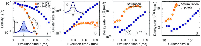
Figure 1: Time evolution of the controlled-dynamics’ fidelity and the corresponding effective cluster-size of correlated spins as a measure of the scrambling of information. (a) The fidelity decay $f(t)=\text{Tr}\left[I_{z}(t)I_{z}^{0}(t)\right]/\mathrm{Tr}\left(I_{z}^{2}\right)$ is shown for two perturbation strengths, for the perturbation Hamiltonian $\Sigma=\mathcal{H}_{dd}$. The strongest perturbation shows an exponential decay law for times > 0.3 ms. (inset) A MQC-fidelity $f_{M}(t)$ between the perturbed dynamics $I_{z}(t)$ and the ideal –non-perturbed– dynamics $I_{z}^{0}(t)$ as a function of the coherence order $M$. The enclosed area gives the global fidelity $f(t)$. (b) Evolution of the cluster-size of correlated spins $K(t)$ determined from the second moment of the MQC-fidelity (inset). The number of correlated spins $K(t)$ defines the “coherence length” on which the density matrices are comparable. For the weakest perturbations, the cluster size grows indefinitely, while for the strongest ones, $K(t)$ reaches a stationary value –an effect we call localization–. (c) The instantaneous decoherence rate $\chi^{\prime}(p,t)=\frac{d\chi}{dt}(p,t)$ of the fidelity $f(t)$ as a function of time $t$. The exponential decay regimen of $f(t)$ is manifested here when the decoherence rate $\chi^{\prime}(t)$ achieves a constant value. (d) The instantaneous decoherence rate $\chi^{\prime}$ as a function of the cluster-size $K$. The plateau of $\chi^{\prime}(t)$ that appears when the cluster size $K(t)$ localizes in (c), here is manifested by the accumulation of points at the end of the curve $\chi^{\prime}(K)$.

This fidelity is identical to the Loschmidt Echo [30, 31, 32] by choosing the observable magnetization $I_{z}$ equal to the initial magnetization. We first evolve the system with the perturbed evolution operator $U_{p}(t)$ and then we time-reverse the evolution with the unperturbed evolution operator $U_{0}^{\dagger}(t)$. The observable signal $\propto\mathrm{Tr}\left(U_{0}^{\dagger}U_{p}I_{z}U_{p}^{\dagger}U_{0}\cdot I_{z}\right)$ gives the many-body Loschmidt-Echo

$$f(t)=\mathrm{Tr}\left(U_{0}^{\dagger}U_{p}I_{z}U_{p}^{\dagger}U_{0}\cdot I_{z}\right)/\mathrm{Tr}\left(I_{z}^{2}\right)$$ (5)

that is equal to the fidelity after considering cyclic permutations (see Appendix C).

IV Multiple-Quantum Fidelity and OTOC

We perform a partial tomography of the density matrix fidelity by applying a rotation operation $\phi_{z}=e^{i\phi I_{z}}$ between the forward $U_{p}(t)$ and backward evolution $U_{0}^{\dagger}(t)$. The global fidelity becomes

$$f_{\phi}(t)=\mathrm{Tr}\left(U_{0}^{\dagger}\phi_{z}U_{p}I_{z}U_{p}^{\dagger}\phi_{z}^{\dagger}U_{0}\cdot I_{z}\right)/\mathrm{Tr}\left(I_{z}^{2}\right)\\ =\mathrm{Tr}\left[I_{z}(t)\phi_{z}^{\dagger}I_{z}^{0}(t)\phi_{z}\right]/\mathrm{Tr}\left(I_{z}^{2}\right)\\ ={\textstyle\sum_{M}}e^{i\phi M}f_{M}(t)/\mathrm{Tr}\left(I_{z}^{2}\right),$$ (6)

where we decompose it into the partial MQC inner-products

$$f_{M}(t)=\mathrm{Tr}\left[I_{z,M}(t)I_{z,M}^{0}(t)\right]/\mathrm{Tr}\left(I_{z}^{2}\right)$$ (7)

of different coherence orders $M$. The overlap $f_{M}(t)$ quantifies the deviation of the density operator elements with a given $M$ of the perturbed evolution from the ideal ones (see Appendix D).

If the perturbation strength $p=0$, Equation (6) gives a conventional OTOC

$$f_{\phi}(p=0,t) =\left\langle I_{z}^{0}(t)\phi_{z}^{\dagger}I_{z}^{0}(t)\phi_{z}\right\rangle_{\beta=0}$$ (8)

$$=\left\langle\phi_{z}(t)I_{z}\phi_{z}^{\dagger}(t)I_{z}\right\rangle_{\beta=0},$$ (9)

with $\phi_{z}(t)=U_{0}(t)\phi_{z}U_{0}^{\dagger}(t)$. Here $\left\langle\cdot\right\rangle_{\beta=0}=\mathrm{Tr\left(\cdot\right)/\mathrm{Tr}}\left(I_{z}^{2}\right)$ is an expectation value normalized to its value at $t=0$ if the system is assumed at infinite temperature (see Appendix E). It quantifies the scrambling into the system of the local information stored in the initial state $\rho(0)$ [27, 6]. The components $f_{M}(p=0,t)=\mathrm{Tr}\left[I_{z,M}^{0}(t)I_{z,M}^{0}(t)\right]/\mathrm{Tr}\left(I_{z}^{2}\right)$ are the amplitudes of the MQC spectrum representing the distribution of coherences (non-diagonal terms in the eigenbasis of $I_{z}$) of the density matrix that were built by the control Hamiltonian $\mathcal{H}_{0}$ [26, 11]. The second-moment of the MQC spectrum $f_{M}(p=0,t)$ provides the average cluster-size of correlated spins

$$\tfrac{K_{0}(t)}{2} =\sum_{M}M^{2}f_{M}(p=0,t)$$ (10)

$$=\mathrm{\mathrm{Tr}}\left([I_{z}^{0}(t),I_{z}]^{\dagger}[I_{z}^{0}(t),I_{z}]\right)/\mathrm{Tr}\left(I_{z}^{2}\right)$$ (11)

at the evolution time $t$ [26, 11, 27, 28] (see Appendix E). The expression $\mathrm{\mathrm{Tr}}\left([I_{z}^{0}(t),I_{z}]^{\dagger}[I_{z}^{0}(t),I_{z}]\right)/\mathrm{Tr}\left(I_{z}^{2}\right)=\left\langle[I_{z}^{0}(t),I_{z}]^{\dagger}[I_{z}^{0}(t),I_{z}]\right\rangle_{\beta=0}$ is a commutator OTOC that quantifies the degree by which the initially commuting operators $I_{z}^{0}(t)$ and $I_{z}$ fail to commute at time $t$ due to the scrambling of information induced by the spin-spin interactions of $\mathcal{H}_{0}$ [27, 28].

Considering the perturbed evolution ($p\neq 0$), the fidelity $f_{\phi}(t)$ is a more general OTOC that quantifies the deviation of the information scrambling induced by $\mathcal{H}(p)$ with respect to the one driven by $\mathcal{H}_{0}$. This is seen from the second moment of $f_{M}(t)$,

$$\sum_{M}M^{2}f_{M}(t)=\mathrm{Tr}\left([I_{z}(t),I_{z}]^{\dagger}[I_{z}^{0}(t),I_{z}]\right)/\mathrm{Tr}\left(I_{z}^{2}\right),$$ (12)

that based on the inner-product between the commutators $[I_{z}(t),I_{z}]$ and $[I_{z}^{0}(t),I_{z}]$ gives the degree of non-commutation shared by the evolved states $I_{z}^{0}(t)$ and $I_{z}(t)$ with respect to $I_{z}$ (see Appendix E). Since $\sum_{M}f_{M}=f(t)=\mathrm{Tr}\left[I_{z}(t)I_{z}^{0}(t)\right]/\mathrm{Tr}\left(I_{z}^{2}\right)$ decays as a function of time, the cluster size of correlated spins is determined from the normalized second moment

$$K(t)=\tfrac{2\sum_{M}M^{2}f_{M}(t)}{\sum_{M}f_{M}(t)}.$$ (13)

As the perturbation Hamiltonians $\mathcal{H}_{dd}$ and $\mathcal{H}_{z}$ do not generate MQC by themselves, the OTOC of Eq. (12) provides the scrambling of information by the spin-spin interactions of $\mathcal{H}_{0}$ that survived the perturbation effects. Based on the second moment of $f_{M}(t)$, $K(t)$ defines a “coherence length” between the two scrambling dynamics of information in terms of an average hamming weight [39, 36, 38] for the fidelity of the density matrix. Therefore $K(t)$ quantifies how comparable the perturbed and unperturbed density matrix dynamics are as a function of the coherence order $M$. This coherence length $K(t)$ defines the effective cluster-size of correlated spins on which the density matrices are comparable based on the inner-product $f_{M}(t)=\mathrm{Tr}\left[I_{z,M}(t)I_{z,M}^{0}(t)\right]/\mathrm{Tr}\left(I_{z}^{2}\right)$ as a kind of fidelity in Eq. (12). In experimental implementations of quantum simulations, there are always uncontrolled perturbations [12] (see Appendix F). These interactions add extra terms to $\Sigma$ that are responsible for the fidelity decay even when the controlled perturbation is $p=0$. This can be interpreted as the effective perturbation strength is no null.

We measure the time evolution of the MQC-fidelities $f_{M}(t)$ for different perturbations to determine the global fidelity $f(t)$ and the effective cluster-size $K(t)$. Both are shown in Fig. 1(a) and (b), respectively, for a weak ($p=0.0017$) and a strong perturbation strength ($p=0.108$) when $\Sigma=\mathcal{H}_{dd}$. The fidelity decays faster as a function of time with increasing perturbation strength. The fidelity decays even in the unperturbed case $p=0$ as decribed above, due to terms that are not included in the Hamiltonian of Eq. (3) (see Appendix F). The perturbation $p=0.0017$ represents a limiting case $p\rightarrow 0$ from which $f(t)$ no longer improves, indicating that the remaining decay is originated by the uncontrolled perturbation sources. The cluster-size $K(t)$ initially grows exponentially as a function of time and then slows down to a power law behavior whose growth-rate reduces with increasing perturbation strength. For strong perturbations $K(t)$ saturates to a value independent of time that decreases with increasing perturbation strength [11]. We call this effect localization of the “coherence length” of the MQC-fidelity that quantifies the “localization” of the scrambling of information shared between the perturbed and ideal dynamics determined from the OTOC of Eq. (12). The fidelity $f(t)$ reaches an exponential decay regimen with a constant rate when the dynamics of $K(t)$ is localized (Fig. 1(a)). Analogous results are observed for $\Sigma=\mathcal{H}_{z}$.

V Fidelity decay rate scaling with the instantaneous coherence length

The fidelity decay

$$f(p,t)=e^{-\chi(p,t)}$$ (14)

is determined by the instantaneous decoherence rate [Fig. 1(c)]

$$\chi^{\prime}(p,t)=\frac{d\chi}{dt}(p,t).$$ (15)

For strong perturbations, the decoherence rate $\chi^{\prime}(t)$ reaches a plateau –a constant value– that depends on the perturbation strength when the dynamics of $K(t)$ is localized. However, for weak perturbations when the dynamics of $K(t)$ does not evidence localization, this plateau is not manifested. Consistently when localization effects are observed, $\chi^{\prime}(K)$ evidences an accumulation of points as shown in Fig. 1(d). This demonstrates that the saturation of $\chi^{\prime}(t)$ and $K(t)$ occur at the same time. Moreover, the experimental results show that $\chi^{\prime}(K)\propto K^{\alpha}$ for long times, indicating that the fidelity decay rate is determined by a scrambling rate defined by the instantaneous effective cluster-size of correlated spins $K$.

Figure 2 shows $\chi^{\prime}$ as a function of $K$, now for both perturbation Hamiltonians $\Sigma=\mathcal{H}_{dd}$ and $\Sigma=\mathcal{H}_{z}$ and different perturbation strengths. The power law functional form $\chi^{\prime}(K)\sim K^{\alpha}$ holds for all the considered cases. The exponents $\alpha$ are shown in Fig. 2(c). They give qualitative different limiting values for the localized (strong perturbation) and delocalized curves (weak perturbation). For the strongest perturbations, the asymptotic behavior at long times shows a power law $\chi^{\prime}(K)\sim K^{\alpha_{\infty}}$, where $\alpha_{\infty}=0.96\pm 0.02$ for the perturbation $\mathcal{H}_{dd}$ and $\alpha_{\infty}=0.91\pm 0.03$ for $\mathcal{H}_{z}$, both near to a linear scaling. However, the exponents drop for the weakest perturbations as $p\rightarrow 0$. In the limit we obtain $\alpha_{0}=(0.48\pm 0.03)$ for both $\Sigma$ with the asymptotic behavior $\chi^{\prime}(K)\sim K^{\alpha_{0}}$. We expect this exponent to be determined by the uncontrolled perturbation effects that were not accounted in the experimental quantum simulations (see Appendix F).

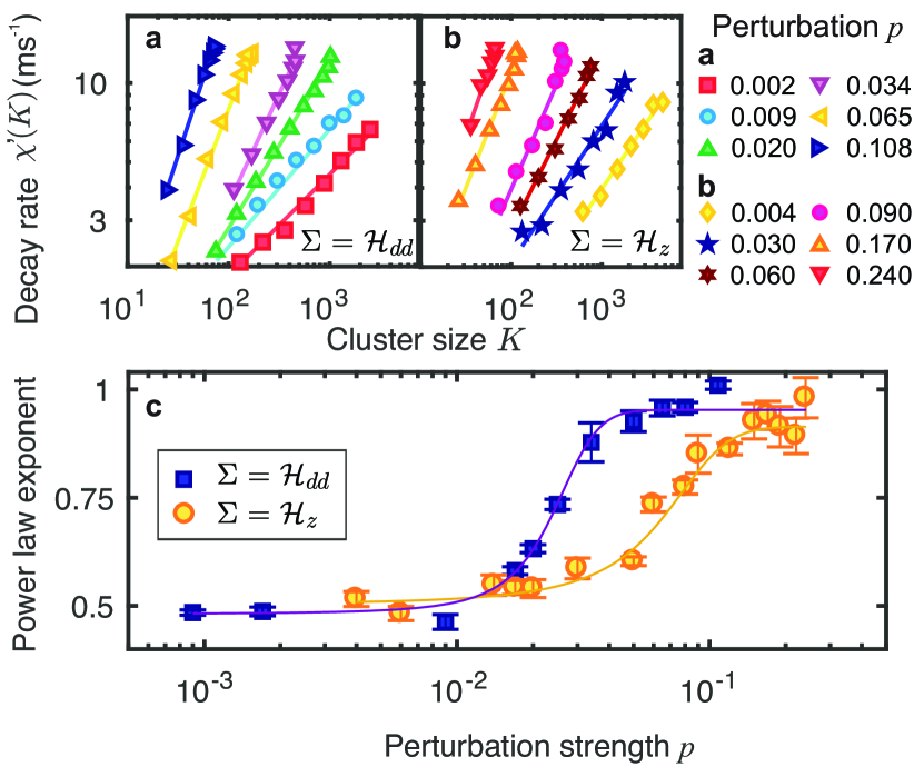
Figure 2: Instantaneous decoherence rate $\chi^{\prime}$ as a function of the effective cluster-size $K$. The two perturbation Hamiltonians are considered (a) $\Sigma=\mathcal{H}_{dd}$ and (b) $\Sigma=H_{z}$. At long times, the fidelity decay rate is driven by the scrambling rate $\chi^{\prime}(K)\sim K^{\alpha}$ given by the instantaneous cluster-size, with a power-law exponent that depends on the perturbation strength $p$. (c) The power law exponent $\alpha$ decreases with decreasing the perturbations strength, showing two plateau values at the weakest ($\alpha_{0}$) and at strongest perturbation ($\alpha_{\infty}$). To estimate $\alpha_{0}$ and $\alpha_{\infty}$, we fit $\alpha(p)$ with a sigmoid function (solid line).

VI Scaling transition on the fidelity decay law: a perturbation threshold

To quantitatively analyze the different scaling laws determined by the exponent $\alpha$, we implement finite-time scaling techniques typically used to describe localization-delocalization transitions from finite-time experimental data [44, 45, 11]. We consider the evolution time dependence implicit on the cluster-size $K(t)$. We use the following Ansatz for the scaling behavior at long times (see Appendix G)

$$\chi^{\prime}(p,K)\sim K^{k_{1}}F\left[(p_{c}-p)K^{-k_{2}}\right],$$ (16)

where $F$ is an arbitrary function. The constants $k_{1}$ and $k_{2}$ are determined to reproduce the asymptotic behavior at weak and strong perturbations. This assumption leads to the functional regimes $\chi^{\prime}\sim(p_{c}-p)^{s}K^{\alpha_{0}}$ for $p<p_{c}$ and $\chi^{\prime}\sim(p-p_{c})^{-2\nu}K^{\alpha_{\infty}}$, for $p>p_{c}$ at long times. We determine the critical exponents from the asymptotic experimental data, obtaining $s=(-0.911\pm 0.004$), $\nu=(-0.57\pm 0.03)$ for $\Sigma=\mathcal{H}_{dd}$, and $s=(-0.93\pm 0.06)$, $\nu=(-0.47\pm 0.05)$ for $\Sigma=\mathcal{H}_{z}$. We then find the scaling factor $\zeta(p)$ that produces an universal scaling (see Appendix G). Rescaled curves of $\chi^{\prime}$ as a function of $K$ that collapse into the universal scaling curve are shown in Fig. 3(a),(b). The two branches of the functional behavior, evidence two dynamical phases for the decoherence effect on the controlled quantum operation characterized by the scrambling dynamics given by $K(t)$.

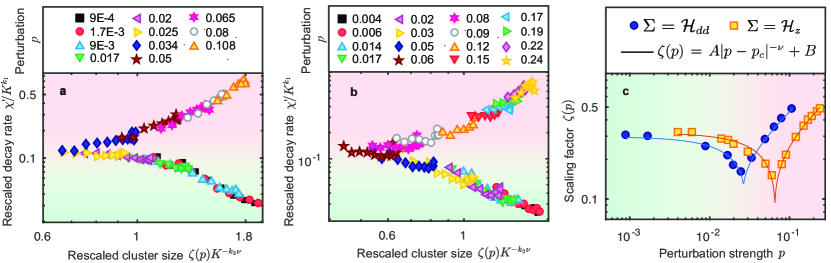
Figure 3: Decoherence scaling transition between two dynamical regimes of the fidelity decay evidenced by the finite-time scaling analysis. Scalings for both perturbation Hamiltonians (a) $\Sigma=\mathcal{H}_{dd}$ and (b) $\Sigma=\mathcal{H}_{z}$ are shown. (c) The corresponding scaling factors $\zeta(p)$ and their fittings to the function $\zeta(p)=A|p-p_{c}|^{-\nu}+B$. In the case of $\Sigma=\mathcal{H}_{dd}$, the critical exponents are $\nu=(-0.57\pm 0.03)$ and $s=(-0.93\pm 0.06)$ and the critical perturbation $p_{c}=(0.026\pm 0.001)$. For $\Sigma=\mathcal{H}_{z}$, the critical perturbation is $p_{c}=(0.065\pm 0.01)$, and the critical exponents are $\nu=(-0.47\pm 0.05)$ and $s=(-0.93\pm 0.06)$. The curves of $\zeta(p)$ are normalized to satisfy $\zeta(p_{\infty})=\sqrt{\chi^{\prime}(K)/K^{\alpha_{\infty}}}$, where $p_{\infty}=0.108$ for $\Sigma=\mathcal{H}_{dd}$ and $p_{\infty}=0.24$ for $\Sigma=\mathcal{H}_{z}$ are the largest perturbation strength used in the experiments.

The scaling factors $\zeta(p)$ that lead to the universal scalings for both perturbations are consistent with the single parameter Ansatz of Eq. (16) that predicts a functional form $\zeta(p)\sim(p-p_{c})^{-\nu}$ (Fig. 3(c)). The critical perturbation $p_{c}=(0.026\pm 0.001)$ for $\Sigma=\mathcal{H}_{dd}$ is in agreement with previous experimental values that evidenced a localization-delocalization transition in the dynamics of the cluster-size $K(t)$ on the same system[11]. This coincidence of $p_{c}$ suggests that the critical effects in the dynamics behavior of $K(t)$ and $\chi^{\prime}(K)$ might be related by a common physical phenomenon. However, the scaling transition of the exponent $\alpha$ is not determined by the scaling transition of the dynamic behavior of $K(t)$. The effect of the localization behavior on $\chi^{\prime}(K)$ is the accumulation of points at the end of the curve as shown in Fig. 1(d), but does not determine the power law exponent on the relation $\chi^{\prime}(K)\sim K^{\alpha}$.

VII Conclusion

In summary, we have designed an experiment to quantify the deviation of a perturbed dynamics from the ideal one based on monitoring the scrambling of information with MQC and OTOCs. Analyzing many-body Loschmidt Echoes, we demonstrated that the fidelity decay rate of the ideal quantum information dynamics is driven by the instantaneous cluster-size $K(t)$ of correlated spins, which quantifies the information spreading induced by the control operation. This instantaneous cluster-size $K(t)$ is an OTOC that gives the common number of correlated spins shared by the ideal $I_{z}^{0}(t)$ and perturbed $I_{z}(t)$ dynamics. The fidelity decay shows a transition between two different scaling laws that depend on the scrambling rate $K^{\alpha}$, whose power law exponent changes suddenly as a function of the perturbation strength. By reducing the perturbation strength below a threshold, the exponent $\alpha$ drops abruptly below 1 and there is no inherent limit to the number of qubits that can be controlled as expected by the ideal dynamics. This is encouraging as the dynamical decoherence rate does not scale linearly with the system size. Although the transition from one regime to another is smooth due to the finite evolution time of the experimental data, the finite-time scaling indicates the existence of the two dynamical regimes. The fact that the controlled dynamics is more resilient to perturbations if they are below a finite critical value $p_{c}$, is also promising for allowing reliable quantum control of large quantum systems. The presented methods provide new avenues for characterizing the control of many-body systems out-of-equilibrium with realistic -imperfect- operations for designing novel quantum technologies.

Appendix A Initial state

The spin system is described as an ensemble of states with the density operator. The initial state is a thermal state at room temperature where $k_{B}T\gg\hbar\omega_{z}$. Therefore, the initial density matrix is approximated by [42]

$$\rho(0)=\frac{e^{-\frac{\hbar\omega_{z}I_{z}}{k_{B}T}}}{\text{tr{\hbox{\left\{ e^{-\frac{\hbar\omega_{z}I_{z}}{k_{B}T}}\right\} }} }}\approx\left(\mathbb{I}+\frac{\hbar\omega_{z}}{k_{\mathrm{B}}T}I_{z}\right)/\mathrm{Tr}\left\{\mathbb{I}\right\}.$$ (17)

Notice that as our experimental observable is the spin operator $I_{z}$, then as $\text{Tr}\left(I_{z}\mathbb{I}\right)=0$, the unity operator $\mathbb{I}$ in Eq. (17) does not contribute to an observable signal. Then as the NMR signal is $S(t)\propto\text{Tr}\left(I_{z}\rho(t)\right)=\text{Tr}\left(I_{z}U(t)I_{z}U(t)\right)\times\left(\frac{\hbar\omega_{z}}{k_{\mathrm{B}}T}/\mathrm{Tr}\left\{\mathbb{I}\right\}\right)$, it gives the time evolution of the operator $I_{z}$ multiplied by a constant term.

Appendix B Hamiltonian engineering

The effective Hamiltonian of Eq. (3) is generated by concatenating short evolution periods $e^{-i\tau_{0}\mathcal{H}_{0}}$ and $e^{-i\tau_{\Sigma}\Sigma}$ of duration $\tau_{0}$ and $\tau_{\Sigma}$ respectively. We get $e^{-i\tau_{0}\mathcal{H}_{0}}e^{-\tau_{\Sigma}\Sigma}=e^{-i\tau_{c}\left[(1-p)\mathcal{H}_{0}+p\Sigma\right]+\mathcal{O}[(\tau_{c}d)^{2}]}$ if the cycle time $\tau_{c}=\tau_{0}+\tau_{\Sigma}\ll d^{-1}$, where $d\approx 13$kHz is the full-width-half-maximum of the resonance line determined by the homogeneous broadening induced by the dipolar coupling between the spins. Here $p=\tau_{\Sigma}/\tau_{c}$ is controlled by adjusting $\tau_{\Sigma}.$ Then based on the Suzuki-Trotter expansion, the evolution operator $U_{p}(t)$ is achieved by applying repetitively $N$ cycles $e^{-i\tau_{0}\mathcal{H}_{0}}e^{-\tau_{\Sigma}\Sigma}$ of duration $\tau_{c}$,

$$U_{p}(N\tau_{c})\approx e^{-i\left[(1-p)\mathcal{H}_{0}+p\Sigma\right]N\tau_{c}},$$ (18)

where the evolution time $t=N\tau_{c}$.

To engineer the double quantum Hamiltonian $\mathcal{H}_{0}$, we use the 8-pulse sequence developed in Refs. [46, 26]. We applied $\pi/2$ RF pulses in the $x$ direction of duration $\tau_{p}=3.24\,\mu\mathrm{s}$, with delays $\Delta=2\,\mu$s and $\Delta^{\prime}=2\Delta+\tau_{p}$. The evolution operator of one cycle is

$$U_{0}(\tau_{0})=e^{-i\Delta/2\mathcal{H}_{dd}}X^{-1}e^{-i\Delta^{\prime}\mathcal{H}_{dd}}X^{-1}e^{-i\Delta\mathcal{H}_{dd}}X^{-1}\times\\ \times e^{-i\Delta^{\prime}\mathcal{H}_{dd}}X^{-1}e^{-i\Delta\mathcal{H}_{dd}}Xe^{-i\Delta^{\prime}\mathcal{H}_{dd}}Xe^{-i\Delta\mathcal{H}_{dd}}\times\\ \times Xe^{-i\Delta^{\prime}\mathcal{H}_{dd}}Xe^{-i\Delta/2\mathcal{H}_{dd}},$$

where $X$ is the $\pi/2$-pulse in the $x$ direction. The duration of the pulse-sequence’s cycle in our experiments was $\tau_{0}=62.88\,\mu\mathrm{s}.$ Again if $\tau_{0}d\ll 1$, $U(\tau_{0})$ approximates to

$$U_{0}(\tau_{0})\approx e^{-i\tau_{0}\mathcal{H}_{0}}.$$ (19)

The perturbation $\Sigma=\mathcal{H}_{dd}$ was prepared by a free-evolution period of duration $\tau_{\Sigma}$ following the cycle of $\mathcal{H}_{0}$ of duration $\tau_{0}$ [29, 11]. The perturbation $\Sigma=\mathcal{H}_{z}=\Delta\omega_{z}I_{z}$ is produced by phase-shifts of the pulses that generate the $\mathcal{H}_{0}$ Hamiltonian by following the protocol proposed in Ref. [38]. The $n$-th cycle of the 8-pulse sequence that generates $\mathcal{H}_{0}$ is shifted by an angle $(n-1)\varphi$. Then, the evolution operator for the $n$-th cycle is

$$U_{n}(\tau_{0})=e^{-iI_{z}(n-1)\varphi}\,e^{-i\mathcal{H}_{0}\tau_{0}}\,e^{iI_{z}(n-1)\varphi},$$ (20)

and the concatenation of $N$ cycles is then

$$U_{p}(N\,\tau_{0}) =U_{N}...\,U_{1}$$ (21)

$$=e^{-iN\varphi I_{z}}\left[e^{-i\tau_{0}\mathcal{H}_{0}}e^{i\varphi I_{z}}\right]^{N}$$

$$=e^{-iN\varphi I_{z}}\left[e^{-i\tau_{0}\mathcal{H}_{0}}e^{i\tau_{\Sigma}dI_{z}}\right]^{N}$$ (22)

$$\simeq e^{-iN\varphi I_{z}}e^{-i\tau_{c}N\left[(1-p)\mathcal{H}_{0}+p\Delta\omega_{z}I_{z}\right]},$$ (23)

where we have defined $\tau_{\Sigma}=\varphi/d$ and $\Delta\omega_{z}=-d$. As in the case $\Sigma=\mathcal{H}_{dd}$, $p=\tau_{\Sigma}/\tau_{c}$. The extra phase $e^{-iN\varphi I_{z}}$ is corrected by increasing the codification phase $\phi$ for determining the MQC spectrum in an angle $N\varphi$ [38]. The resulting effective Hamiltonian is then

$$\mathcal{H}(p)\simeq(1-p)\mathcal{H}_{0}+p\mathcal{H}_{z}.$$ (24)

Appendix C Fidelity

We implement a Loschmidt Echo as a measure of the fidelity between the ideal density matrix evolving with $U_{0}(t)=e^{-it\mathcal{H}_{0}}$ and the perturbed one evolving with $U_{p}(t)=e^{-it\mathcal{H}(p)}$. The resulting NMR signal is therefore $S(t)\propto\mathrm{Tr}\left[U_{0}^{\dagger}U_{p}\rho(0)U_{p}^{\dagger}U_{0}\cdot I_{z}\right]\propto\mathrm{Tr}\left[U_{p}I_{z}U_{p}^{\dagger}U_{0}I_{z}U_{0}^{\dagger}\right]=\mathrm{Tr}\left[I_{z}(t)I_{z}^{0}(t)\right]$. We normalized the experimental data in Fig. 1(a) at $t=0$ to obtain the fidelity $f(t)=S(t)/S(0)=\frac{\mathrm{Tr}\left(I_{z}(t)I_{z}^{0}(t)\right)}{\mathrm{Tr}\left(I_{z}^{2}\right)}$.

Appendix D Determination of the MQC-spectrum and the MQC-fidelity

The double-quantum Hamiltonian of Eq. (2) flips simultaneously two spins with the same orientation. Taking into account the selection rules of the transitions, the $z$-component of the magnetization $M_{z}$ changes by $M=\Delta M_{z}=\pm 2$ to add or subtract $\Delta K=\pm 1$ to the number of correlated spins $K$ among which the coherence is shared [43]. Therefore the change of coherence order allows to probe the number of correlated spins as a witness of the quantum information spreading [26]. The spin density matrix after evolving with the evolution operator $U_{0}(t)$ from the initial state can be decomposed on the coherence orders as

$$\rho(t)=\sum_{M}\sum_{m_{j}-m_{i}=M}\rho_{ij}(t)\left|m_{i}\right\rangle\left\langle m_{j}\right|=\sum_{M}\rho_{M}(t),$$ (25)

where the operator $\rho_{M}(t)=\sum_{m_{j}-m_{i}=M}\rho_{ij}(t)$ contains all the elements of the density operator involving the coherences of order $M$. Then a rotation $\phi_{z}=e^{-i\phi I_{z}}$ of a phase $\phi$ around the $z$-axis, changes the density operator to

$$\rho\left(\phi,t\right)=\phi_{z}\rho(t)\phi_{z}^{-1}=\sum_{M}e^{iM\phi}\rho_{M}(t).$$ (26)

The fidelity $f_{\phi}(t)$ with the proper normalization results then

$$f_{\phi}(t) =\mathrm{Tr}\left[\phi_{z}U_{p}I_{z}U_{p}^{\dagger}\phi_{z}U_{0}\cdot I_{z}U_{0}^{\dagger}\right]/\mathrm{Tr}\left(I_{z}^{2}\right)$$ (27)

$$=\mathrm{Tr}\left[I_{z}(\phi,t)I_{z}^{0}(t)\right]/\mathrm{Tr}\left(I_{z}^{2}\right)$$ (28)

$$=\sum_{M^{\prime}}e^{iM\phi}\mathrm{Tr}\left[I_{z,M}(t)I_{z,M}^{0}(t)\right]/\mathrm{Tr}\left(I_{z}^{2}\right)$$ (29)

$$=\sum_{M}e^{iM\phi}f_{M},$$ (30)

where $f_{M}(t)=\mathrm{Tr}\left[I_{z,M}(t)I_{z,M}^{0}(t)\right]/\mathrm{Tr}\left(I_{z}^{2}\right)$ is a inner-product that with a proper normalization can be interpreted as a MQC fidelity. The MQC-fidelity is therefore determined by performing a Fourier transform on $\phi$ of the echo signal $f_{\phi}(t)$. Similarly, when $p=0$, $f_{M}(p=0,t)=\mathrm{Tr}\left[I_{z,M}^{0}(t)I_{z,M}^{0}(t)\right]/\mathrm{Tr}\left(I_{z}^{2}\right)$ gives the MQC-spectrum [26].

Appendix E OTOCs and the effective cluster-size $K(t)$

At $p=0$, the fidelity $f_{\phi}(p=0,t)=\text{Tr}\left[\phi_{z}(t)I_{z}\phi_{z}^{\dagger}(t)I_{z}\right]/\mathrm{Tr}\left(I_{z}^{2}\right)=\left\langle\phi_{z}(t)I_{z}\phi_{z}^{\dagger}(t)I_{z}\right\rangle_{\beta=0}$ is a conventional OTOC, where the expectation value $\left\langle O(t)\right\rangle_{\beta}=\text{Tr}\left\{O(t)\rho_{\beta}\right\}/\text{Tr}\left\{O(0)\rho_{\beta}\right\}$ of the operator $O(t)$ is normalized at $t=0$, where $\rho_{\beta}=e^{-\beta\mathcal{H}}/\text{Tr}(e^{-\beta\mathcal{H}})$ is the equilibrium density matrix of the system at the inverse temperature $\beta$ [34, 47, 28, 38]. In our case the OTOC provides information of the system at infinite temperature with $\beta=0$, i.e. $\rho_{\beta=0}=\mathbb{I}/\text{Tr}(\mathbb{I})$. The fidelity $f_{\phi}(p=0,t)$ quantifies the degree of non-commutation of $\phi_{z}(t)$ and $I_{z}$ according to the relation

$$f_{\phi}(p=0,t)=1-\frac{1}{2}\text{Tr}\left([\phi_{z}(t),I_{z}]^{\dagger}[\phi_{z}(t),I_{z}]\right)/\mathrm{Tr}\left(I_{z}^{2}\right).$$ (31)

Performing a Taylor expansion of $f_{\phi}(p=0,t)$ for small $\phi$, we get the second moment of the MQC-spectrum [48, 28]

$$m_{2}^{0}(t) =\sum_{M}M^{2}f_{M}(p=0,t)$$ (32)

$$=\text{Tr}\left([I_{z}^{0}(t),I_{z}]^{\dagger}[I_{z}^{0}(t),I_{z}]\right)/\mathrm{Tr}\left(I_{z}^{2}\right).$$ (33)

It is possible to deduce from $m_{2}^{0}$ the number of correlated spins $K_{0}$ by making assumptions on the MQC spectrum $f_{M}$ [48]. The most extended model was proposed by Baum et. al [26, 49] that gives a Gaussian distribution for $f_{M}$ as a function of $M$, where $K_{0}(t)=2m_{2}^{0}(t)$ is determined from the width of the Gaussian distribution. The exact value of $K_{0}$ will depend on the assumed model for the MQC distribution [48].

When $p\neq 0$, $f_{\phi}(t)=\text{Tr}\left(I_{z}(t)\phi_{z}^{\dagger}I_{z}^{0}(t)\phi_{z}\right)/\mathrm{Tr}\left(I_{z}^{2}\right)=\left\langle I_{z}(t)\phi_{z}^{\dagger}I_{z}^{0}(t)\phi_{z}\right\rangle_{\beta=0}$ is a more general OTOC [47] that satisfies

$$f_{\phi}(t)=\\ =\left\{\text{Tr}\left(I_{z}(t)I_{z}^{0}(t)\right)-\text{$\frac{1}{2}$Tr}\left([I_{z}(t),\phi_{z}]^{\dagger}[I_{z}^{0}(t),\phi_{z}]\right)\right\}/\mathrm{Tr}\left(I_{z}^{2}\right)\\ =f_{\phi=0}(t)-\text{$\frac{1}{2}$Tr}\left([I_{z}(t),\phi_{z}]^{\dagger}[I_{z}^{0}(t),\phi_{z}]\right)/\mathrm{Tr}\left(I_{z}^{2}\right).$$ (34)

Expanding $f_{\phi}(t)$ in powers of $\phi$, equivalently as was done for obtaining Eq. (32), we obtain the second moment of the MQC distribution $f_{M}(t)$

$$m_{2}(t) =\sum_{M}M^{2}f_{M}(t)$$ (35)

$$=\text{Tr}\left([I_{z}(t),I_{z}][I_{z}^{0}(t),I_{z}]^{\dagger}\right)/\mathrm{Tr}\left(I_{z}^{2}\right).$$ (36)

The second moment $m_{2}(t)$ quantifies the overlap between the scrambling of the ideal evolution $I_{z}^{0}(t)$ and the perturbed evolution $I_{z}(t)$, determined by the inner-product between the corresponding commutators $[I_{z}^{0}(t),I_{z}]$ and $[I_{z}(t),I_{z}]$ respectively. Due to the effect of the perturbation, the total intensity of the MQC spectrum $\sum_{M}f_{M}(t)=f_{\phi=0}(t)$ decreases as a function of time, so the second moment $m_{2}$ must be normalized by $f_{\phi=0}(t)$ to determine the width of the MQC distribution. In analogy with the case $p=0$, the effective number of correlated spins is $K(t)=2m_{2}(t)/f_{\phi=0}(t)$.

Appendix F Intrinsic Decoherence effects

The ideal form of the effective Hamiltonian $\mathcal{H}_{0}$ of Eq. (2) is based on an 0-th order approximation using average Hamiltonian theory [50]. It can only be achieved if the dipolar couplings $d_{ij}$ are time independent, all pulses of the NMR sequences are ideal and the condition $\tau_{c}=\tau_{0}+\tau_{\Sigma}\ll d^{-1}$ is good enough. However, typically these couplings are time dependent due to thermal fluctuations, and the pulses are not ideal. In addition, there are non-secular terms neglected in Eq. (1), and they might also contribute to the quantum dynamics. All these effects introduce extra terms in the effective Hamiltonian $\mathcal{H}$ of Eq. (3) and in $\mathcal{H}_{0}$ of Eq. (2). These extra perturbation terms produce decoherence effects on ms time scales during the quantum simulations, even for $p=0$. These decoherence effects reduce the detected signal and the overall fidelity $f(t)$. Then also the MQC-spectrum is attenuated with an overall global factor. However, on this study, this decoherence effects do not cause localization of the information scrambling dynamics on the time scale of our experiments when $p\rightarrow 0$ (see Fig. 2, black squares). When $p\neq 0$, we quantify the scrambling rate $K$ from the second moment of Eq. (12) generated by $\mathcal{H}_{0}$ after a time-reversed evolution under $\mathcal{-H}_{0}$. This means that these clusters have survived the decoherence effects. Therefore, the non-equilibrium many-body dynamics observed by the OTOC of Eq. (12), thus reflects the coherent quantum dynamics generated by the engineered Hamiltonians. We notice that, the experimentally observed quantum dynamics occurs over times scales much shorter than the spin-lattice relaxation time, $T_{1}\approx 1$ sec, so we also neglect the effect of thermalization with the lattice. Therefore, when the controlled perturbation is set to $p=0$, we consider that the effective perturbation is not null and we determine the cluster size of correlated spins using $K(t)=\tfrac{2\sum_{M}M^{2}f_{M}(t)}{\sum_{M}f_{M}(t)}$ as for the $p\neq 0$ case.

Appendix G Finite-time scaling procedure

To implement the finite-time scaling technique [44, 45, 11], we used the asymptotic experimental data for $p\rightarrow 0$, that shows that $\chi^{\prime}(p\rightarrow 0,K)\propto K^{\alpha_{0}}$ for long times. Then we used the asymptotic experimental data for the largest perturbation strengths $p_{\infty}=0.108$ for $\Sigma=\mathcal{H}_{dd}$ and $p_{\infty}=0.24$ for $\Sigma=\mathcal{H}_{z}$, that in these cases $\chi^{\prime}(p_{\infty},K)\propto K^{\alpha_{\infty}}$ is satisfied for long times. If there is a transition from these two regimes at a perturbation $p_{c}$, then close to the transition one expects a power law dependence on $(p-p_{c})$ for the decoherence rate [44, 45, 11]. We then consider the following asymptotic functional dependence at long times

$$\chi^{\prime}(p,K)\sim\begin{cases}(p_{c}-p)^{s}K^{\alpha_{0}}&p<p_{c}\\ (p-p_{c})^{-2\nu}K^{\alpha_{\infty}}&p>p_{c},\end{cases}$$ (37)

where the time dependence is implicit on $K$.

We use the single-parameter Ansatz for the scaling behavior at long times in order to find the scaling of the curves of Fig. 2, consistently with previous experimental findings [11]

$$\chi^{\prime}(K,p)\sim K^{k_{1}}F\left[(p_{c}-p)K^{k_{2}}\right].$$ (38)

Here $F(x)$ is an arbitrary function. Based on the asymptotic behavior of the experimental data, if $p<p_{c}$, then $\chi^{\prime}\sim(p_{c}-p)^{s}K^{\alpha_{0}}$, implying that $F(x)\sim x^{s}$ and

$$k_{1}+sk_{2}=\alpha_{0}.$$ (39)

Then for $p>p_{c}$, $\chi^{\prime}\sim(p_{c}-p)^{-2\nu}K^{\alpha_{\infty}}$ implies $F(x)\sim(-x)^{-2\nu}$ and

$$k_{1}-2k_{2}\nu=\alpha_{\infty}.$$ (40)

We estimate $p_{c}$ from Fig. 2(c) and we found that the experimental data satisfy these asymptotic limits for $p\leq 0.009$ and $p\geq 0.05$ for $\mathcal{H}_{dd}$, and for $p\leq 0.05$ and $p\geq 0.17$ for $\mathcal{H}_{z}$. We obtain $s=(-0.911\pm 0.004$), $\nu=(-0.57\pm 0.03)$ for $\Sigma=\mathcal{H}_{dd}$, and $s=(-0.93\pm 0.06)$, $\nu=(-0.47\pm 0.05)$ for $\Sigma=\mathcal{H}_{z}$.

The scaling hypothesis is then generalized to

$$\chi^{\prime}(K,p)\sim K^{k_{1}}\Phi\left[\zeta(p)K^{-k_{2}\nu}\right]$$ (41)

for accounting for the intermediate time regimes, where $\Phi(x)$ and $\zeta(p)$ again are arbitrary functions. This equation is less restrictive than Eq. (38) but includes it. Using the obtained critical exponents, and the values of $\alpha_{0}$ and $\alpha_{\infty}$ obtained from the asymptotic limits in Fig. 2(c), we get $k_{1}=0.69\pm 0.05$ and $k_{2}\nu=-0.13\pm 0.02$ for $\Sigma=\mathcal{H}_{dd}$ and $k_{1}=0.69\pm 0.07$ and $k_{2}\nu=-0.11\pm 0.02$ for $\Sigma=\mathcal{H}_{z}$ from Eqs. (39) and (40). The scaling behavior is then found by a proper determination of $\zeta(p)$.

To find the scaling factor $\zeta(p)$, we plot the curves of $\frac{\chi^{\prime}}{K^{k_{1}}}$ as a function of $K^{-k_{2}\nu}$, and shift them by $\zeta(p)$ to overlap with each other for different values of $p$ in such a way that they generate a single curve as in Fig. 3. A single curve is only obtained if the experimental data is consistent with the scaling assumptions. To assure the consistency of the scaling determination, according to Eqs. (16) and (41), then the scaling factor must satisfy

$$\zeta(p)\sim(p-p_{c})^{-\nu}.$$ (42)

The curves of $\zeta(p)$ are normalized to satisfy $\zeta(p_{\infty})=\sqrt{\chi^{\prime}(K)/K^{\alpha_{\infty}}}$, for the largest perturbation strength used in the experiments $p_{\infty}=0.108$ for $\Sigma=\mathcal{H}_{dd}$ and $p_{\infty}=0.24$ for $\Sigma=\mathcal{H}_{z}$. We then fit the experimental data with the function $\zeta(p)=A|p-p_{c}|^{-\nu}+B$, where the parameter $B$ accounts for the finite time experimental data and external decoherence process that smooth the transition [44, 45, 11]. We observed the consistency of the fitted curves and the extracted critical exponents with the assumed single-parameter Ansatz of Eq. (16). The critical perturbations from these fittings are then $p_{c}=(0.026\pm 0.006)$ and $(0.065\pm 0.01)$ for $\mathcal{H}_{dd}$ and $\mathcal{H}_{z}$ respectively. These values are consistent with the ones estimated from Fig. 2(c).

We emphasize that the critical behavior of the scaling exponent $\alpha$ is a new physical phenomenon, which cannot be deduced from the localized-delocalized transition previously reported in $K(t)$ [11]. When the decoherence rate $\chi^{\prime}$ is parameterized as a function of time, then localization of $K(t)$ implies localization of $\chi^{\prime}(t),$ as it is shown in Fig. 1(c). Instead, the decoherence rate parameterized as a function of the systems size $\chi^{\prime}(K)\propto K^{\alpha}$ provides an scaling exponent $\alpha$ that is independent of the temporal behavior of $K$. Thus localization of $K(t)$ has no implications in $\alpha.$

References

- Eisert et al. [2015] J. Eisert, M. Friesdorf, and C. Gogolin, Nat. Phys. 11, 124 (2015).
- Abanin et al. [2019] D. A. Abanin, E. Altman, I. Bloch, and M. Serbyn, Rev. Mod. Phys. 91, 021001 (2019).
- Martinez et al. [2016] E. A. Martinez, C. A. Muschik, P. Schindler, D. Nigg, A. Erhard, M. Heyl, P. Hauke, M. Dalmonte, T. Monz, P. Zoller, and R. Blatt, Nature 534, 516 (2016).
- Swingle [2018] B. Swingle, Nat. Phys. 14, 988 (2018).
- Friis et al. [2018] N. Friis, O. Marty, C. Maier, C. Hempel, M. Holzäpfel, P. Jurcevic, M. B. Plenio, M. Huber, C. Roos, R. Blatt, and B. Lanyon, Phys. Rev. X 8, 021012 (2018).
- Lewis-Swan et al. [2019] R. J. Lewis-Swan, A. Safavi-Naini, A. M. Kaufman, and A. M. Rey, Nat. Rev. Phys. 1, 627 (2019).
- Zhang et al. [2017] J. Zhang, G. Pagano, P. W. Hess, A. Kyprianidis, P. Becker, H. Kaplan, A. V. Gorshkov, Z.-X. Gong, and C. Monroe, Nature 551, 601 (2017).
- Bernien et al. [2017] H. Bernien, S. Schwartz, A. Keesling, H. Levine, A. Omran, H. Pichler, S. Choi, A. S. Zibrov, M. Endres, M. Greiner, V. Vuletić, and M. D. Lukin, Nature 551, 579 (2017).
- Neill et al. [2018] C. Neill, P. Roushan, K. Kechedzhi, S. Boixo, S. V. Isakov, V. Smelyanskiy, A. Megrant, B. Chiaro, A. Dunsworth, K. Arya, R. Barends, B. Burkett, Y. Chen, Z. Chen, A. Fowler, B. Foxen, M. Giustina, R. Graff, E. Jeffrey, T. Huang, J. Kelly, P. Klimov, E. Lucero, J. Mutus, M. Neeley, C. Quintana, D. Sank, A. Vainsencher, J. Wenner, T. C. White, H. Neven, and J. M. Martinis, Science 360, 195 (2018).
- Krojanski and Suter [2004] H. G. Krojanski and D. Suter, Phys. Rev. Lett. 93, 090501 (2004).
- Álvarez et al. [2015] G. A. Álvarez, D. Suter, and R. Kaiser, Science 349, 846 (2015).
- Suter and Álvarez [2016] D. Suter and G. A. Álvarez, Rev. Mod. Phys. 88, 041001 (2016).
- Wang et al. [2017] Y. Wang, M. Um, J. Zhang, S. An, M. Lyu, J.-N. Zhang, L.-M. Duan, D. Yum, and K. Kim, Nat. Photonics 11, 646 (2017).
- Trotzky et al. [2012] S. Trotzky, Y.-A. Chen, A. Flesch, I. P. McCulloch, U. Schollwöck, J. Eisert, and I. Bloch, Nat. Phys. 8, 325 (2012).
- Schindler et al. [2013] P. Schindler, M. Müller, D. Nigg, J. T. Barreiro, E. A. Martinez, M. Hennrich, T. Monz, S. Diehl, P. Zoller, and R. Blatt, Nat. Phys. 9, 361 (2013).
- Landsman et al. [2019] K. A. Landsman, C. Figgatt, T. Schuster, N. M. Linke, B. Yoshida, N. Y. Yao, and C. Monroe, Nature 567, 61 (2019).
- Sar et al. [2012] T. v. d. Sar, Z. H. Wang, M. S. Blok, H. Bernien, T. H. Taminiau, D. M. Toyli, D. A. Lidar, D. D. Awschalom, R. Hanson, and V. V. Dobrovitski, Nature 484, 82 (2012).
- Souza et al. [2012] A. M. Souza, G. A. Álvarez, and D. Suter, Phys. Rev. A 86, 050301(R) (2012).
- Taminiau et al. [2014] T. H. Taminiau, J. Cramer, T. v. d. Sar, V. V. Dobrovitski, and R. Hanson, Nat. Nanotechnol. 9, 171 (2014).
- Zhang and Suter [2015] J. Zhang and D. Suter, Phys. Rev. Lett. 115, 110502 (2015).
- Schweigler et al. [2017] T. Schweigler, V. Kasper, S. Erne, I. Mazets, B. Rauer, F. Cataldini, T. Langen, T. Gasenzer, J. Berges, and J. Schmiedmayer, Nature 545, 323 (2017).
- Lukin et al. [2019] A. Lukin, M. Rispoli, R. Schittko, M. E. Tai, A. M. Kaufman, S. Choi, V. Khemani, J. Léonard, and M. Greiner, Science 364, 256 (2019).
- Brydges et al. [2019] T. Brydges, A. Elben, P. Jurcevic, B. Vermersch, C. Maier, B. P. Lanyon, P. Zoller, R. Blatt, and C. F. Roos, Science 364, 260 (2019).
- Buluta and Nori [2009] I. Buluta and F. Nori, Science 326, 108 (2009).
- Georgescu et al. [2014] I. M. Georgescu, S. Ashhab, and F. Nori, Rev. Mod. Phys. 86, 153 (2014).
- Baum et al. [1985] J. Baum, M. Munowitz, A. N. Garroway, and A. Pines, J. Chem. Phys. 83, 2015 (1985).
- Garttner et al. [2017] M. Garttner, J. G. Bohnet, A. Safavi-Naini, M. L. Wall, J. J. Bollinger, and A. M. Rey, Nat. Phys. 13, 781 (2017).
- Gärttner et al. [2018] M. Gärttner, P. Hauke, and A. M. Rey, Phys. Rev. Lett. 120, 040402 (2018).
- Álvarez and Suter [2010] G. A. Álvarez and D. Suter, Phys. Rev. Lett. 104, 230403 (2010).
- Peres [1984] A. Peres, Phys. Rev. A 30, 1610 (1984).
- Pastawski et al. [2000] H. Pastawski, P. Levstein, G. Usaj, J. Raya, and J. Hirschinger, Physica A Stat. Mech. Appl. 283, 166 (2000).
- Jacquod and Petitjean [2009] P. Jacquod and C. Petitjean, Adv. Phys. 58, 67 (2009).
- Yan et al. [2020] B. Yan, L. Cincio, and W. H. Zurek, Phys. Rev. Lett. 124, 160603 (2020).
- Maldacena et al. [2016] J. Maldacena, S. H. Shenker, and D. Stanford, J. High Energy Phys. 2016, 106.
- Li et al. [2017] J. Li, R. Fan, H. Wang, B. Ye, B. Zeng, H. Zhai, X. Peng, and J. Du, Phys. Rev. X 7, 031011 (2017).
- Niknam et al. [2020] M. Niknam, L. F. Santos, and D. G. Cory, Phys. Rev. Res. 2, 13200 (2020).
- Sánchez et al. [2020] C. M. Sánchez, A. K. Chattah, K. X. Wei, L. Buljubasich, P. Cappellaro, and H. M. Pastawski, Phys. Rev. Lett. 124, 030601 (2020).
- Wei et al. [2019] K. X. Wei, P. Peng, O. Shtanko, I. Marvian, S. Lloyd, C. Ramanathan, and P. Cappellaro, Phys. Rev. Lett. 123, 090605 (2019).
- Wei et al. [2018] K. X. Wei, C. Ramanathan, and P. Cappellaro, Phys. Rev. Lett. 120, 070501 (2018).
- Fan et al. [2017] R. Fan, P. Zhang, H. Shen, and H. Zhai, Sci. Bull 62, 707 (2017).
- García-Mata et al. [2018] I. García-Mata, M. Saraceno, R. A. Jalabert, A. J. Roncaglia, and D. A. Wisniacki, Phys. Rev. Lett. 121, 210601 (2018).
- Slichter [1990] C. P. Slichter, Principles of magnetic resonance (Springer-Verlag Berlin Heidelberg, 1990).
- Munowitz et al. [1987] M. Munowitz, A. Pines, and M. Mehring, J. Chem. Phys. 86, 3172 (1987).
- Chabé et al. [2008] J. Chabé, G. Lemarié, B. Grémaud, D. Delande, P. Szriftgiser, and J. C. Garreau, Phys. Rev. Lett. 101, 255702 (2008).
- Lemarié et al. [2009] G. Lemarié, J. Chabé, P. Szriftgiser, J. C. Garreau, B. Grémaud, and D. Delande, Phys. Rev. A 80, 043626 (2009).
- Warren et al. [1979] W. Warren, S. Sinton, D. Weitekamp, and A. Pines, Phys. Rev. Lett. 43, 1791 (1979).
- Kitaev and Suh [2018] A. Kitaev and S. J. Suh, J. High Energ. Phys. 2018 (5), 183.
- Khitrin [1997] A. Khitrin, Chem. Phys. Lett. 274, 217 (1997).
- Baum and Pines [1986] J. Baum and A. Pines, J. Am. Chem. Soc. 108, 7447 (1986).
- Haeberlen and Waugh [1968] U. Haeberlen and J. S. Waugh, Phys. Rev. 175, 453 (1968).