Path Imputation Strategies for Signature Models of Irregular Time Series

Abstract

The signature transform is a ‘universal nonlinearity’ on the space of continuous vector-valued paths, and has received attention for use in machine learning on time series. However, real-world temporal data is typically observed at discrete points in time, and must first be transformed into a continuous path before signature techniques can be applied. We make this step explicit by characterising it as an imputation problem, and empirically assess the impact of various imputation strategies when applying signature-based neural nets to irregular time series data. For one of these strategies, Gaussian process (GP) adapters, we propose an extension (GP-PoM) that makes uncertainty information directly available to the subsequent classifier while at the same time preventing costly Monte-Carlo (MC) sampling. In our experiments, we find that the choice of imputation drastically affects shallow signature models, whereas deeper architectures are more robust. Next, we observe that uncertainty-aware predictions (based on GP-PoM or indicator imputations) are beneficial for predictive performance, even compared to the uncertainty-aware training of conventional GP adapters. In conclusion, we have demonstrated that the path construction is indeed crucial for signature models and that our proposed strategy leads to competitive performance in general, while improving robustness of signature models in particular.

1 Introduction

Originally described by Chen, [5, 6, 7] and popularised in the theory of rough paths and controlled differential equations [32, 14, 31], the signature transform, also known as the path signature or simply signature, acts on a continuous vector-valued path of bounded variation, and returns a graded sequence of statistics, which determine a path up to a negligible equivalence class. Moreover, every continuous function of a path can be recovered by applying a linear transform to this collection of statistics [3, Proposition A.6]. This ‘universal nonlinearity’ property makes the signature a promising nonparametric feature extractor in both generative and discriminative learning scenarios. Further properties include the signature’s uniqueness [20], as well as factorial decay of its higher order terms [32]. These theoretical foundations have been accompanied by outstanding empirical results when applying signatures to clinical time series classification tasks [40, 34].

Due to their similarities, we may hope that tools that apply to continuous paths can also be applied to multivariate time series. But since multivariate time series are not continuous paths, one first needs to construct a continuous path before signature techniques are applicable. Previous work [27, 3, 12] characterised this construction as an embedding problem, and typically considered it a minor technical detail. This is exacerbated by the—perfectly sensible—behaviour of software for computing the signature [39, 22], which commonly considers a continuous piecewise linear path as an input, described by its sequence of knots, i.e. values. Since such sequences resemble a sequence of data, the signature is sometimes interpreted as operating on sequences of data rather than on paths [3, 27]. By contrast, here we show that considering the path construction process is crucial for achieving competitive predictive performance: we reinterpret the task of constructing a continuous path, turning it from an embedding problem to an imputation problem, which we call path imputation.

While previous research concerning the signature transform focused on its excellent theoretical properties, such as sampling independence [3, Proposition A.7], our findings show that this does not necessarily correspond to empirical performance. We perform a thorough investigation of multiple imputation schemes in combination with various models that can potentially employ signatures. Furthermore, motivated by the fact that missingness itself can be informative for time series classification [42], we propose a novel imputation strategy: an extension of Gaussian process adapters [29, 16], which exploits uncertainty information during each prediction step and which is beneficial for signature models, but also of independent interest. We make our code available under https://osf.io/bg9cw/?view_only=5193e93118d84a5f9be4f261df4c0a06.

2 Related work

A key motivation for this work is the use of the signature transform in machine learning: recent work [8, 26, 45, 28, 46, 37, 35] typically employed the signature transform as a nonparametric feature extractor, on top of which a model is learnt. A growing body of work has also investigated how to integrate the signature transform more tightly with neural networks; Reizenstein, [38], Liao et al., [30], and Bonnier et al., [3] all study how to use the signature transform (or variants thereof) within typical neural network models. Chevyrev and Oberhauser, [9], Király and Oberhauser, [25] study how the signature transform may be used to define a kernel—i.e. a symmetric, positive definite function that is typically used as a similarity measure—on path space, while Toth and Oberhauser, [44] show how this kernel may be used to define a Gaussian process. In much of this work, data has been converted into a continuous path via linear interpolation. Some authors [8, 12] have additionally considered ‘rectilinear’ interpolation, which is similar. Levin et al., [27] present the ‘time-joined transformation’, which is a hybrid of the two, such that the resulting path exhibits a causal dependence on the data. However, to our knowledge, no prior work has regarded (and empirically investigated) this as an imputation problem.

Imputation schemes

The general problem of imputing data is well-known and well-studied, and we will not attempt to describe it here; see for example Gelman and Hill, [18, Chapter 25]. Imputation methods typically only fill in missing discrete data points, and do not attempt to impute the underlying continuous path. Gaussian process adapters [29], by contrast, are capable of imputing a full continuous path, from which we may sample arbitrarily. Hence, this framework will be considered more closely in this paper. We note that there are also other approaches that perform imputation end-to-end with a downstream classifier [43] and methods that skip the imputation step altogether based on recently-proposed Neural-ODE like architectures [41, 23], variants of recurrent neural networks [4] or set functions [21]. However, the scope of this work is to specifically assess the impact of path imputations for the signature, hence we deem the larger comparison including imputation-free scenarios interesting for future work, while it bypasses the central point of this paper.

3 Background: Signature transform and Gaussian process adapters

Path signatures

Let $f=(f_{1},\dots,f_{d})\colon[a,b]\to\mathbb{R}^{d}$ be a continuous, piecewise differentiable path. Then the signature transform up to depth $N$ is

$$\mathrm{Sig}^{N}(f)=\left(\left(\underset{\,a<t_{1}<\cdots<t_{k}<b}{\int\cdots\int}\prod_{j=1}^{k}\frac{\mathrm{d}f_{i_{j}}}{\mathrm{d}t}\left(t_{j}\right)\mathrm{d}t_{1}\cdots\mathrm{d}t_{k}\right)_{1\leq i_{1},\ldots,i_{k}\leq d}\right)_{1\leq k\leq N}.$$ (1)

This definition can be extended to paths of bounded variation by replacing these integrals with Stieltjes integrals with respect to each $f_{i_{j}}$. In brief, the signature transform may be interpreted as extracting information about order and area of a path. One may interpret its terms as ‘the area/order of one channel with respect to some collection of other channels’. To give an explicit example: first level terms simply describe the increment of the path with respect to one channel, whereas second-order terms are related to the Levy area of the path, as shown for a one-dimensional example in Figure 1.

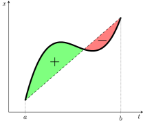
Figure 1: Given a path (bold), its Levy area is its signed area with respect to the chord joining its endpoints.

For an exposition on the properties of the signature transform and its use in machine learning, please refer to Chevyrev and Kormilitzin, [8] or Bonnier et al., [3, Appendix A]. For building more intuition, in Section A.6.1 of the appendix, we compare the signature to more well-known transforms.

Computing the signature transform

Continuous piecewise linear paths are the paths of choice, computationally speaking, due to the fact that this is the only case for which efficient algorithms for computing the signature transform are known [22].

This is not a serious hurdle when one wishes to compute the signature of a path $f$ that is not piecewise linear—as the signature of piecewise linear approximations to $f$ will tend towards the signature of $f$ as the quality of the approximation increases—but it does enforce this requirement on our imputation schemes. Thus, all of the imputation schemes we examine will first seek to select a collection of points in data space (not necessarily only where we had data before), and for computing the signature we join them up into a piecewise linear path.

Notation

We define the space of time series over a set $A$ by

$$\mathcal{S}(A)=\{((t_{1},x_{1}),\ldots,(t_{n},x_{n}))\,|\,t_{i}\in\mathbb{R},x_{i}\in A,n\in\mathbb{N},\text{ such that }t_{1}\leq\cdots\leq t_{n}\}.$$ (2)

Furthermore, let $\mathcal{Y}$ be a set and let $\mathcal{X}_{j}=\mathbb{R}$ for $j\in\{1,\ldots,d\}$ and $d\in\mathbb{N}$. Then we assume that we observe a dataset of labelled time series $(\mathbf{x}_{k},y_{k})$ for $k\in\{1,\ldots,N\}$, where $\mathbf{x}_{k}\in\mathcal{S}(\mathcal{X}^{*})$ and $y_{k}\in\mathcal{Y}$, with $\mathcal{X}^{*}=\prod_{j=1}^{d}(\mathcal{X}_{j}\cup\{*\})$ and $*$ representing no observation. We similarly define $\mathcal{X}=\prod_{j=1}^{d}\mathcal{X}_{j}$. Thus, $\mathcal{X}$ is the data space, while $\mathcal{X}^{*}$ is the data space allowing missing data, and $\mathcal{Y}$ is the set of labels.

Gaussian process adapter

Some of the imputation schemes we consider are based on the uncertainty aware-framework of multi-task Gaussian process adapters [29, 16]. Let $\mathcal{W},\mathcal{H}$ be some sets. Let $\ell\colon\mathcal{Y}\times\mathcal{Y}\to[0,\infty)$ be a loss function. Let $F\colon\mathcal{X}^{[a,b]}\times\mathcal{W}\to\mathcal{Y}$, be some (typically neural network) model, with $\mathcal{W}$ interpreted as a space of parameters. Let

$$\mu\colon[a,b]\times\mathcal{S}(\mathcal{X}^{*})\times\mathcal{H} \to\mathcal{X}$$

$$\Sigma\colon[a,b]\times[a,b]\times\mathcal{S}(\mathcal{X}^{*})\times\mathcal{H} \to\mathcal{X}$$

be mean and covariance functions, with $\mathcal{H}$ interpreted as a space of hyperparameters. The dependence on $\mathcal{S}(\mathcal{X}^{*})$ is used to represent conditioning on observed values.

Then the goal is to solve

$$\operatorname*{arg\,min}_{\mathbf{w}\in\mathcal{W},\bm{\eta}\in\mathcal{H}}\sum_{k=1}^{N}\overbrace{\rule{0.0pt}{14.22636pt}\mathbb{E}_{\mathbf{z}_{k}\sim\mathcal{N}\left(\mu(\cdot,\mathbf{x}_{k},\eta),\Sigma(\cdot,\cdot,\mathbf{x}_{k},\eta)\right)}\big{[}\ell(F(\mathbf{z}_{k},\mathbf{w}),y_{k})\big{]}}^{\text{$E_{k}$}}.$$ (3)

As this expectation is typically not tractable, it is estimated by MC sampling with $S$ samples, i.e.

$$E_{k}\approx\frac{1}{S}\sum_{s=1}^{S}\ell(F(\mathbf{z}_{s,k},\mathbf{w}),y_{k}),$$ (4)

where

$$\mathbf{z}_{s,k}\sim\mathcal{N}\left(\mu(\,\cdot\,,\mathbf{x}_{k},\eta),\Sigma(\,\cdot\,,\,\cdot\,,\mathbf{x}_{k},\eta)\right).$$ (5)

Alternatively, one may forgo allowing the uncertainty to propagate through $F$ by instead passing the posterior mean directly to $F$; this corresponds to solving

$$\operatorname*{arg\,min}_{\mathbf{w}\in\mathcal{W},\bm{\eta}\in\mathcal{H}}\sum_{k=1}^{N}\ell(F(\mu(\,\cdot\,,\mathbf{x}_{k},\eta),\mathbf{w}),y_{k}).$$ (6)

4 Path imputations for signature models

Signatures act on continuous paths. However, in real-world applications, temporal data typically appears as a discretised collection of measurements, potentially irregularly-spaced and asynchronously observed. To apply the signature to this data, it first has to be converted into a continuous path. We believe this step to have a significant impact on the resulting signature, and thus also on models employing the signature. To assess this hypothesis, we explicitly treat this transformation as a path imputation, i.e. a mapping of the form $\phi\colon\mathcal{S}(\mathcal{X}^{*})\to(\mathbb{R}\times\mathcal{X})^{[a,b]}.$

Task

We aim to learn a function $g\colon\mathcal{S}(\mathcal{X}^{*})\to\mathcal{Y}$, which decomposes to $g=F\circ\phi$, where $F$ refers to a classifier, mapping from $(\mathbb{R}\times\mathcal{X})^{[a,b]}\times\mathcal{W}$ to $\mathcal{Y}$. Given a loss function $\ell$ and a set of $p$ path imputation strategies, ${\Phi}=(\phi_{i})_{i=1}^{p}$, we seek to minimise the objective:

$$\operatorname*{arg\,min}_{\phi_{i}\in\Phi,\mathbf{w}\in\mathcal{W}}\quad\mathbb{E}_{(\mathbf{x},y)\sim P(\mathcal{S}(\mathcal{X}^{*}),\mathcal{Y})}\left[\ell(g(\mathbf{x};\phi_{i},\mathbf{w}),y)\right]$$ (7)

Even though Equation (7) could be formulated more implicitly (i.e. without any explicit imputation step), this formulation enables us to make explicit how the signature transform ‘interprets’ the raw data for downstream classification tasks. We further motivate this need for assessing the path construction in Section A.5 by showing that a single imputed value can affect the Levy area which is computed with the signature.

Path imputation strategies

For our analysis, we consider the following set of strategies for path imputation, namely (1) linear interpolation, (2) forward filling, (3) indicator imputation, (4) zero imputation, (5) causal imputation, and (6) Gaussian process adapters (GP). Strategies 1–5 can be seen as a fixed preprocessing step, whereas GP adapters (strategy 6) are optimised end-to-end with the downstream task. For more details regarding these strategies, please refer to Section A.2 in the appendix. As indicated in Section 3, for computing the signature efficiently (i.e. computed in terms of standard tensor operations [3, Proposition A.3]), the imputed time series are transformed into piecewise linear paths beforehand.

Figure 2: Overview of our proposed extension of GP adapters, GP-PoM, leveraging both posterior moments (mean and variance). In comparison, the conventional GP adapter feeds MC samples (faded colours in the background) drawn from the GP posterior into the classifier.

GP adapter with posterior moments

For conventional GP adapters, one major drawback with the formulations of Li and Marlin, [29] and Futoma et al., [16], as described in Equation (3), is that approximating the expectation outside of the loss function with MC sampling is expensive. During prediction, Li and Marlin, [29] proposed to overcome this issue by sacrificing the uncertainty in the loss function and to simply pass the posterior mean, as in Equation (6). To address both points, we propose to instead also pass the posterior covariance of the Gaussian process to the classifier $F$. This saves the cost of MC sampling whilst explicitly providing $F$ with uncertainty information during the prediction. However, the full covariance matrix may become very large, and it is not obvious that all interactions are relevant to the subsequent classifier. This is why we simplify matters by taking the posterior variance at every point, and concatenate it with the posterior mean at every point, to produce a path whose evolution also captures the uncertainty at every point:

$$\tau \colon[a,b]\times\mathcal{S}(\mathcal{X}^{*})\times\mathcal{H}\to\mathcal{X}\times\mathcal{X}$$ (8)

$$\tau \colon t,\mathbf{x},\eta\mapsto(\mu(t,\mathbf{x},\eta),\Sigma(t,t,\mathbf{x},\eta)).$$ (9)

This corresponds to solving

$$\operatorname*{arg\,min}_{\mathbf{w}\in\mathcal{W},\bm{\eta}\in\mathcal{H}}\sum_{k=1}^{N}\ell(F(\tau(\,\cdot\,,\mathbf{x}_{k},\eta),\mathbf{w}),y_{k}),$$ (10)

where instead now $F\colon(\mathcal{X}\times\mathcal{X})^{[a,b]}\times\mathcal{W}\to\mathcal{Y}$. As this approach leverages information from both posterior moments (mean and variance), we refer to it as posterior moments GP adapter, or short GP-PoM. Figure 2 gives an overview of GP-PoM. In our context of interest, when $F$ is a signature model, it is now straightforward to compute the signature of the Gaussian process, simply by querying many points to construct a piecewise linear approximation to the process. The choice of kernel has non-trivial mathematical implications for this procedure: for example if a Matérn 1/2 kernel is chosen, then the resulting path is not of bounded variation and the definition of the signature transform given in Equation (1) does not hold, and rough path theory [32] must instead be invoked to define the signature transform. However, in this work we use RBF kernels, and therefore, this caveat does not apply to our case.

5 Experiments

We first introduce our experimental setup (datasets and model architectures) before presenting and discussing quantitative results.

Datasets and preprocessing

We classify time series from four real-world datasets: (i) PenDigits[11], (ii) CharacterTrajectories[11], (iii) LSST[1], and (iv) Physionet2012[19]. For dataset statistics and necessary filtering steps, please refer to Section A.3 in the appendix. Moreover, to efficiently compute the signature, we sample the imputed path in a fixed time resolution, resulting in a piecewise linear path. For time series that are not irregularly spaced (this applies to all datasets but Physionet2012), we employ two types of random subsampling as an additional preprocessing step, namely (1) ‘Random’: Missing at random; on the instance level, we discard 50% of all observations. (2) ‘Label-based’: Missing not at random; for each class, we uniformly sample missingness frequencies between $40\%$ and $60\%$. Since PenDigits consists of particularly short time series (8 steps, 2 dimensions), we use more moderate frequencies of $30\%$ and $20$–$40\%$, respectively, for discarding observations. Finally, we standardise all time series channels using the empirical mean and standard deviation as determined on the entire training split.

Models

We study the following models: (1) Sig, a simple signature model that involves a linear augmentation, the signature transform (signature block) and a final module of dense layers, (2) RNN, an RNN model using GRU cells [10], (3) RNNSig, which extends the signature transform to a window-based stream of signatures, and where the final neural module is a GRU sliding over the stream of signatures, and (4) DeepSig, a deep signature model sequentially employing two signature blocks featuring augmentation and signature transforms, following Bonnier et al., [3]. Please refer to Supplementary Section A.4 for more details about the architectures and implementations. We use the ‘Signatory’ package to calculate the signature transform [22], and implemented all GP adapters using the ‘GPyTorch’ framework [17].

Training and evaluation

We use the predefined training and testing splits for each dataset, separating $20\%$ of the training split as a validation set for hyperparameter tuning. For each setting, we run a randomised hyperparameter search of $20$ calls and train each of these fits until convergence (at most 100 epochs; we stop early if the performance on the validation split does not improve for 20 epochs). As for performance metrics, for binary classification tasks, we optimise area under the precision-recall curve (as approximated via average precision) and also report AUROC. For multi-class classification, we optimise balanced accuracy (BAC) and additionally report accuracy and weighted AUROC (w-AUROC). Having selected the best hyperparameter configuration for each setting, we repeat $5$ fits; for each fit, we select the best model state in terms of the best validation performance, and finally report mean and standard deviation (error bars) of the performance metrics on the testing split.

Table 1: CharacterTrajectories dataset under label-based subsampling. The top three methods are highlighted: bold & underlined, bold, underlined. All measures are reported as percentage points. Balanced accuracy (BAC) is the metric we optimised for. We further report accuracy and weighted AUROC (w-AUROC).

Imputation	Model	w-AUROC	BAC	Accuracy
GP-PoM	DeepSig	$99.582\pm 0.671$	$95.155\pm 1.501$	$94.958\pm 1.716$
	RNN	$\underline{99.973\pm 0.015}$	$\mathbf{98.161\pm 0.664}$	$\mathbf{98.273\pm 0.602}$
	RNNSig	$99.696\pm 0.089$	$92.778\pm 1.239$	$93.231\pm 1.133$
	Sig	$99.516\pm 0.075$	$88.627\pm 1.416$	$89.011\pm 1.319$
GP	DeepSig	$99.290\pm 0.704$	$89.545\pm 2.996$	$89.368\pm 3.123$
	RNN	$99.970\pm 0.011$	$97.712\pm 0.266$	$97.873\pm 0.251$
	RNNSig	$96.669\pm 2.393$	$65.717\pm 13.691$	$67.052\pm 13.182$
	Sig	$95.283\pm 1.602$	$62.423\pm 6.110$	$63.614\pm 5.958$
causal	DeepSig	$99.940\pm 0.024$	$97.272\pm 0.709$	$97.437\pm 0.620$
	RNN	$99.960\pm 0.010$	$97.239\pm 0.516$	$97.409\pm 0.481$
	RNNSig	$99.523\pm 0.155$	$89.922\pm 2.301$	$90.585\pm 2.186$
	Sig	$95.747\pm 4.957$	$66.307\pm 21.794$	$68.259\pm 20.757$
forward-filling	DeepSig	$99.953\pm 0.041$	$97.956\pm 0.677$	$98.078\pm 0.656$
	RNN	$99.942\pm 0.011$	$96.942\pm 0.486$	$97.159\pm 0.444$
	RNNSig	$99.720\pm 0.071$	$92.568\pm 1.091$	$93.148\pm 1.011$
	Sig	$94.828\pm 8.117$	$67.169\pm 26.338$	$68.649\pm 26.125$
indicator	DeepSig	$\mathbf{\underline{99.988\pm 0.013}}$	$\mathbf{\underline{98.591\pm 0.294}}$	$\mathbf{\underline{98.719\pm 0.263}}$
	RNN	$99.916\pm 0.020$	$96.414\pm 0.406$	$96.671\pm 0.367$
	RNNSig	$99.802\pm 0.032$	$93.787\pm 0.463$	$94.234\pm 0.442$
	Sig	$91.661\pm 10.003$	$56.423\pm 22.796$	$58.384\pm 22.932$
linear	DeepSig	$99.970\pm 0.010$	$\underline{98.051\pm 0.743}$	$\underline{98.217\pm 0.671}$
	RNN	$99.880\pm 0.059$	$96.906\pm 1.314$	$97.117\pm 1.196$
	RNNSig	$99.876\pm 0.035$	$94.848\pm 0.916$	$95.292\pm 0.842$
	Sig	$80.442\pm 18.228$	$31.193\pm 23.962$	$32.326\pm 24.679$
zero	DeepSig	$\mathbf{99.977\pm 0.010}$	$98.030\pm 0.357$	$98.189\pm 0.358$
	RNN	$99.967\pm 0.014$	$97.428\pm 0.572$	$97.549\pm 0.596$
	RNNSig	$99.699\pm 0.132$	$91.752\pm 1.782$	$92.368\pm 1.662$
	Sig	$77.727\pm 23.671$	$37.992\pm 34.456$	$38.955\pm 35.232$

Table 2: PenDigits dataset under label-based subsampling. The top three methods are highlighted: bold & underlined, bold, underlined. All measures are reported as percentage points. Balanced accuracy (BAC) is the metric we optimised for. We further report accuracy and weighted AUROC (w-AUROC)

Imputation	Model	w-AUROC	BAC	Accuracy
GP-PoM	DeepSig	$\underline{99.930\pm 0.032}$	$\mathbf{97.403\pm 0.300}$	$\mathbf{97.381\pm 0.298}$
	RNN	$99.901\pm 0.016$	$96.349\pm 0.297$	$96.306\pm 0.302$
	RNNSig	$99.669\pm 0.073$	$93.022\pm 0.765$	$92.967\pm 0.763$
	Sig	$99.150\pm 0.144$	$88.090\pm 1.493$	$87.999\pm 1.499$
GP	DeepSig	$92.885\pm 1.455$	$60.593\pm 4.092$	$60.476\pm 4.067$
	RNN	$95.170\pm 1.438$	$67.543\pm 4.782$	$67.426\pm 4.790$
	RNNSig	$84.501\pm 1.307$	$42.184\pm 1.977$	$42.141\pm 1.913$
	Sig	$80.312\pm 2.655$	$37.767\pm 3.611$	$37.725\pm 3.646$
causal	DeepSig	$99.241\pm 0.075$	$89.616\pm 0.749$	$89.514\pm 0.747$
	RNN	$99.241\pm 0.098$	$89.496\pm 0.480$	$89.417\pm 0.501$
	RNNSig	$99.298\pm 0.041$	$89.187\pm 0.476$	$89.137\pm 0.494$
	Sig	$98.374\pm 0.065$	$83.205\pm 0.404$	$83.082\pm 0.426$
forward-filling	DeepSig	$99.007\pm 0.072$	$88.205\pm 0.434$	$88.090\pm 0.428$
	RNN	$99.333\pm 0.046$	$89.747\pm 0.406$	$89.657\pm 0.419$
	RNNSig	$99.274\pm 0.015$	$89.788\pm 0.384$	$89.743\pm 0.392$
	Sig	$98.310\pm 0.045$	$83.739\pm 0.421$	$83.625\pm 0.398$
indicator	DeepSig	$\mathbf{\underline{99.960\pm 0.013}}$	$\mathbf{\underline{98.068\pm 0.184}}$	$\mathbf{\underline{98.056\pm 0.185}}$
	RNN	$\mathbf{99.955\pm 0.009}$	$\underline{97.266\pm 0.439}$	$\underline{97.238\pm 0.447}$
	RNNSig	$99.747\pm 0.028$	$93.488\pm 0.616$	$93.408\pm 0.613$
	Sig	$99.410\pm 0.031$	$90.591\pm 0.306$	$90.492\pm 0.308$
linear	DeepSig	$99.458\pm 0.052$	$91.567\pm 0.412$	$91.452\pm 0.416$
	RNN	$99.489\pm 0.093$	$91.608\pm 0.609$	$91.492\pm 0.608$
	RNNSig	$99.446\pm 0.039$	$90.259\pm 0.859$	$90.143\pm 0.869$
	Sig	$98.963\pm 0.084$	$87.254\pm 0.437$	$87.141\pm 0.458$
zero	DeepSig	$99.391\pm 0.071$	$91.121\pm 0.406$	$91.012\pm 0.403$
	RNN	$99.551\pm 0.031$	$91.765\pm 0.283$	$91.670\pm 0.304$
	RNNSig	$99.321\pm 0.033$	$89.543\pm 0.412$	$89.457\pm 0.417$
	Sig	$98.544\pm 0.069$	$84.269\pm 0.445$	$84.185\pm 0.454$

Results

(a) CharacterTrajectories-R

(b) CharacterTrajectories-L

Figure 3: Experimental results visualised for CharacterTrajectories dataset. The bars display performance in terms of balanced accuracy (BAC), whereas the panels indicate the subsampling strategy. Left: Random subsampling (R), right: label-based subsampling (L).

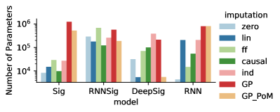
(a) CharacterTrajectories-R

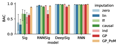
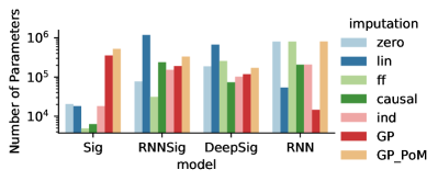
(b) CharacterTrajectories-L

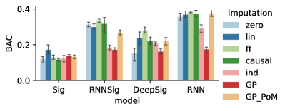
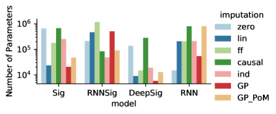
(c) LSST-R

(d) LSST-L

Figure 4: Visualisations for CharacterTrajectories and LSST . The rows indicate datasets and different subsampling schemes (R for Random, L for Label-based). The left column displays the performance metric which was optimzied for: balanced accuracy (BAC), or average precision. The right column indicates the number of trainable parameters which the best model required (as selected in the hyperparameter search).

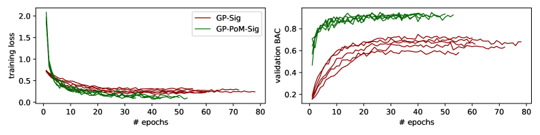
Figure 6: GP-PoM training illustrated for CharacterTrajectories as compared to conventional GP adapter.

In Tables 1 and 2, the results for CharacterTrajectories and PenDigits under label-based subsampling are shown, respectively. For the remaining datasets and subsampling strategies, please refer to Tables 3–7 in the appendix. We observe that both DeepSig as well as the signature-free RNN perform well over many scenarios. In particular, they are impervious to the choice of several imputation schemes in the sense that it does not have a large impact on their predictive performance. However, we also see that certain signature models, in particular Sig, are heavily impacted by the choice of imputation strategy. Figure 3 exemplifies this finding in a barplot visualization; for the remaining visualizations, including the number of parameters of the optimised models, please refer to Supplementary Figures 4 and 5. In the case of CharacterTrajectories, Sig was only able to achieve acceptable performance through our novel GP-PoM strategy. In PenDigits, we encountered issues of numerical stability for the original GP adapter; not so for GP-PoM. Furthermore, we found that GP-PoM tends to converge faster to a better performance than the original GP adapter, as exemplified in Supplementary Figure 6.

6 Discussion

Our findings suggest that the choice of path imputation strategy can drastically affect the performance of signature-based models. We observe this most prominently in ‘shallow’ signature models, whereas deep signature models (DeepSig) are more robust in tackling irregular time series over different imputations—comparable to non-signature RNNs, yet on average being more parameter-efficient.

Overall, we find that uncertainty-aware approaches (indicator imputation and GP-PoM) are beneficial when imputing irregularly-spaced time series for classification. Crucially, uncertainty information has to be accessible during the prediction step. We find that this is indeed not the case for the standard GP adapter (despite the naming of ‘uncertainty-aware framework’), since for each MC sample, the downstream classifier has no access to missingness or uncertainty about the underlying imputation. GP-PoM, our proposed end-to-end imputation strategy, shows competitive classification performance, while considerably improving upon the existing GP adapter. As for limitations, GP-PoM sacrifices the GP adapter’s ability to be explicitly uncertain about its own prediction (due to the variance of the MC sampled predictions), while the subsequent classifier has to be able to handle the doubled feature dimensionality.

Recommendations for the practitioner

When dealing with a challenging time series classification task, we recommend to consider signatures as a powerful tool to encode paths with little loss of information. However, we observe that this comes at a certain cost: since the signature describes continuous paths (and not discrete time series), constructing this path from raw data is a delicate task that can heavily impact the signature and the performance of downstream models. To this end, we recommend using GP-PoM, which explicitly captures uncertainty in the imputed path. Given our findings, indicator imputation is a simple but promising go-to strategy, however we caution its use together with shallow signature models since we observed detrimental effects in terms of predictive performance. Furthermore, when applying signatures in online applications or settings, where during training no data should leak from the future (e.g. in online settings, this could impair performance upon deployment), we recommend to use causal (or time-joined) path imputations: their design specifically prevents leakage from the future, even if the signature interprets the imputations as knots of a piece-wise linear path.

7 Conclusion

The signature transform has recently gained attention for being a promising feature extractor that can be easily integrated to neural networks. As we empirically demonstrated in this paper, the application of signature transforms to real-world temporal data is fraught with pitfalls—specifically, we found the choice of an imputation scheme to be crucial for obtaining high predictive performance. Moreover, by integrating uncertainty to the prediction step, our proposed GP-PoM has demonstrated overall competitive performance and in particular improved robustness in signature models when classifying irregularly-spaced and asynchronous time series.

Broader Impact

Whilst the task of converting observed data into a path in data space is particularly important for signatures, it also arises in the context of, for example, convolutional and recurrent neural networks.

Convolutions are often thought of in terms of discrete sums, but they are perhaps more naturally described as the integral cross-correlation between the underlying data path $f$ and the learnt filter $g_{\theta}$. Given sample points $t_{1},\ldots,t_{n}\in[0,T]$, this integral is then approximated via numerical quadrature:

$$\frac{1}{T}\int_{0}^{T}f(t)g_{\theta}(t)\mathrm{d}t\approx\frac{1}{n}\sum_{i=1}^{n}f(t_{i})g_{\theta}(t_{i}),$$

although the $1/n$ scaling is really only justified in the case that the $t_{i}$ are equally spaced. Thus we see that with convolutions, we are implicitly interpreting the observed data as a path in data space.

Similarly, the connections between dynamical systems and recurrent neural networks are well known [15, 2], and these tend to use a similar setup. For non-signature methods as for signature methods, this implicit usage of data as a path in data space often seems to be swept under the rug, and we have demonstrated that this is deserving further attention.

With respect to ethical considerations, we acknowledge that time series models in general can be used for better or for worse. On top of that, implicit biases underlying models as well as datasets can have unintended harmful consequences. By shedding light on the impact of implicit usage of paths in data space we hope to forward understanding and accountability of black-box models. Even if our work focuses on signature models, we believe that the principle of making underlying assumptions explicit is relevant far beyond this class of models.

8 Acknowledgements

M.M, M.H, and C.B were supported by the SNSF Starting Grant ‘Significant Pattern Mining’. The authors are grateful to Patrick Kidger for valuable discussions, guidance, and code contributions.

Appendix A Appendix

A.1 Further Experiments

Table 3: CharacterTrajectories, random subsampling

Imputation	Model	w-AUROC	BAC	Accuracy
GP-PoM	DeepSig	$99.698\pm 0.393$	$94.011\pm 5.037$	$93.635\pm 5.335$
	RNN	$\underline{99.970\pm 0.011}$	$98.011\pm 0.512$	$98.106\pm 0.508$
	RNNSig	$99.787\pm 0.074$	$93.308\pm 0.960$	$93.844\pm 0.903$
	Sig	$99.578\pm 0.031$	$89.570\pm 0.938$	$89.930\pm 0.914$
GP	DeepSig	$98.994\pm 1.088$	$90.821\pm 2.361$	$90.471\pm 2.347$
	RNN	$99.909\pm 0.032$	$96.276\pm 0.691$	$96.492\pm 0.715$
	RNNSig	$99.400\pm 0.094$	$87.587\pm 2.054$	$88.141\pm 1.959$
	Sig	$94.862\pm 1.779$	$61.280\pm 6.440$	$62.446\pm 6.493$
causal	DeepSig	$99.963\pm 0.023$	$97.774\pm 0.228$	$97.953\pm 0.182$
	RNN	$99.953\pm 0.023$	$97.657\pm 0.720$	$97.813\pm 0.676$
	RNNSig	$99.814\pm 0.044$	$93.268\pm 0.730$	$93.747\pm 0.743$
	Sig	$96.736\pm 0.578$	$71.393\pm 3.784$	$73.245\pm 3.642$
forward-filling	DeepSig	$99.965\pm 0.030$	$97.974\pm 0.381$	$98.120\pm 0.365$
	RNN	$99.954\pm 0.010$	$97.786\pm 0.308$	$97.939\pm 0.281$
	RNNSig	$99.840\pm 0.047$	$94.110\pm 0.774$	$94.596\pm 0.745$
	Sig	$54.308\pm 4.187$	$7.387\pm 2.995$	$7.117\pm 2.417$
indicator	DeepSig	$99.955\pm 0.033$	$\mathbf{98.626\pm 0.500}$	$\mathbf{98.733\pm 0.481}$
	RNN	$99.953\pm 0.024$	$97.502\pm 0.527$	$97.660\pm 0.499$
	RNNSig	$99.755\pm 0.078$	$93.091\pm 1.056$	$93.635\pm 0.952$
	Sig	$66.917\pm 18.306$	$18.481\pm 18.692$	$19.067\pm 19.165$
linear	DeepSig	$\mathbf{\underline{99.984\pm 0.007}}$	$\mathbf{\underline{98.898\pm 0.205}}$	$\mathbf{\underline{98.997\pm 0.201}}$
	RNN	$99.928\pm 0.043$	$97.668\pm 0.897$	$97.786\pm 0.802$
	RNNSig	$99.767\pm 0.037$	$92.754\pm 0.662$	$93.273\pm 0.656$
	Sig	$55.023\pm 6.655$	$9.436\pm 3.349$	$9.958\pm 4.097$
zero	DeepSig	$\mathbf{99.980\pm 0.013}$	$\underline{98.337\pm 0.644}$	$\underline{98.454\pm 0.616}$
	RNN	$99.887\pm 0.052$	$96.004\pm 1.074$	$96.253\pm 1.046$
	RNNSig	$99.685\pm 0.063$	$92.154\pm 0.878$	$92.744\pm 0.820$
	Sig	$96.997\pm 0.388$	$69.963\pm 4.208$	$71.699\pm 4.002$

Table 4: PenDigits, random subsampling

metric	w-AUROC	BAC	Accuracy
GP-PoM	DeepSig	$99.515\pm 0.078$	$92.151\pm 0.555$	$92.098\pm 0.548$
	RNN	$99.564\pm 0.072$	$\underline{92.757\pm 0.735}$	$\underline{92.699\pm 0.733}$
	RNNSig	$98.967\pm 0.253$	$88.148\pm 1.588$	$88.113\pm 1.579$
	Sig	$99.028\pm 0.099$	$87.352\pm 0.898$	$87.290\pm 0.903$
GP	DeepSig	$90.509\pm 0.164$	$54.545\pm 0.426$	$54.513\pm 0.451$
	RNN	$91.961\pm 0.856$	$57.930\pm 2.079$	$57.900\pm 2.088$
	RNNSig	$86.740\pm 0.585$	$46.842\pm 1.255$	$46.867\pm 1.218$
	Sig	$83.511\pm 0.485$	$41.747\pm 0.428$	$41.809\pm 0.425$
causal	DeepSig	$99.096\pm 0.116$	$89.480\pm 0.359$	$89.434\pm 0.362$
	RNN	$99.288\pm 0.066$	$89.526\pm 0.535$	$89.474\pm 0.539$
	RNNSig	$99.165\pm 0.067$	$88.807\pm 0.613$	$88.759\pm 0.617$
	Sig	$97.870\pm 0.224$	$80.065\pm 0.980$	$80.011\pm 0.971$
forward-filling	DeepSig	$99.141\pm 0.068$	$88.974\pm 0.656$	$88.902\pm 0.644$
	RNN	$99.311\pm 0.067$	$90.067\pm 0.247$	$90.029\pm 0.247$
	RNNSig	$99.203\pm 0.063$	$88.930\pm 0.513$	$88.902\pm 0.528$
	Sig	$98.425\pm 0.069$	$84.458\pm 0.468$	$84.374\pm 0.477$
indicator	DeepSig	$\mathbf{99.607\pm 0.059}$	$\mathbf{93.156\pm 0.738}$	$\mathbf{93.087\pm 0.751}$
	RNN	$\mathbf{\underline{99.733\pm 0.044}}$	$\mathbf{\underline{94.124\pm 0.412}}$	$\mathbf{\underline{94.071\pm 0.415}}$
	RNNSig	$99.549\pm 0.041$	$91.604\pm 0.278$	$91.532\pm 0.268$
	Sig	$98.708\pm 0.040$	$84.544\pm 0.538$	$84.505\pm 0.563$
linear	DeepSig	$99.407\pm 0.151$	$91.418\pm 1.075$	$91.366\pm 1.086$
	RNN	$99.510\pm 0.041$	$91.862\pm 0.582$	$91.812\pm 0.594$
	RNNSig	$\underline{99.591\pm 0.036}$	$91.556\pm 0.518$	$91.521\pm 0.539$
	Sig	$99.029\pm 0.094$	$87.116\pm 0.612$	$87.038\pm 0.612$
zero	DeepSig	$99.334\pm 0.077$	$89.774\pm 0.541$	$89.686\pm 0.553$
	RNN	$99.403\pm 0.112$	$90.729\pm 0.618$	$90.698\pm 0.620$
	RNNSig	$99.150\pm 0.046$	$87.948\pm 0.248$	$87.879\pm 0.243$
	Sig	$98.623\pm 0.073$	$83.935\pm 0.382$	$83.905\pm 0.375$

Table 5: LSST, label-based subsampling

Imputation	Model	w-AUROC	BAC	Accuracy
GP-PoM	DeepSig	$64.414\pm 6.770$	$13.857\pm 2.394$	$8.743\pm 2.889$
	RNN	$82.808\pm 4.284$	$29.483\pm 7.106$	$29.781\pm 11.520$
	RNNSig	$82.934\pm 1.495$	$31.751\pm 2.338$	$35.442\pm 3.621$
	Sig	$58.820\pm 1.427$	$13.779\pm 0.535$	$10.187\pm 1.418$
GP	DeepSig	$59.686\pm 3.444$	$13.144\pm 3.924$	$28.333\pm 5.465$
	RNN	$69.269\pm 1.469$	$16.558\pm 0.465$	$33.903\pm 0.356$
	RNNSig	$60.032\pm 0.476$	$16.779\pm 1.559$	$33.627\pm 0.213$
	Sig	$57.381\pm 0.555$	$14.062\pm 1.174$	$24.294\pm 2.135$
causal	DeepSig	$75.336\pm 3.543$	$25.481\pm 5.868$	$39.400\pm 5.824$
	RNN	$84.107\pm 0.606$	$37.762\pm 1.736$	$53.009\pm 1.684$
	RNNSig	$82.343\pm 0.235$	$33.570\pm 2.776$	$50.284\pm 0.973$
	Sig	$58.837\pm 3.205$	$12.262\pm 2.841$	$34.161\pm 1.295$
forward-filling	DeepSig	$77.758\pm 2.562$	$27.473\pm 4.165$	$42.238\pm 5.435$
	RNN	$84.153\pm 0.675$	$38.621\pm 1.618$	$52.976\pm 0.667$
	RNNSig	$82.430\pm 0.439$	$34.078\pm 1.399$	$50.560\pm 0.678$
	Sig	$64.200\pm 0.808$	$14.779\pm 1.184$	$35.255\pm 0.520$
indicator	DeepSig	$\mathbf{95.351\pm 1.044}$	$\mathbf{52.124\pm 2.147}$	$\mathbf{77.283\pm 2.231}$
	RNN	$\mathbf{\underline{98.132\pm 0.242}}$	$\mathbf{\underline{61.893\pm 3.862}}$	$\mathbf{\underline{83.609\pm 1.452}}$
	RNNSig	$82.635\pm 1.816$	$29.122\pm 3.102$	$41.152\pm 2.456$
	Sig	$57.084\pm 0.863$	$12.806\pm 0.951$	$32.620\pm 1.113$
linear	DeepSig	$73.965\pm 3.208$	$21.356\pm 0.745$	$36.504\pm 6.349$
	RNN	$84.931\pm 0.301$	$40.098\pm 0.968$	$\underline{54.023\pm 0.822}$
	RNNSig	$82.883\pm 0.805$	$32.553\pm 1.276$	$49.327\pm 2.426$
	Sig	$66.687\pm 1.812$	$17.340\pm 0.777$	$35.726\pm 0.571$
zero	DeepSig	$75.783\pm 1.217$	$23.598\pm 3.268$	$42.019\pm 1.718$
	RNN	$\underline{87.908\pm 0.952}$	$\underline{40.479\pm 1.890}$	$53.268\pm 2.066$
	RNNSig	$79.432\pm 0.496$	$34.381\pm 1.176$	$46.521\pm 0.446$
	Sig	$52.972\pm 1.080$	$11.951\pm 1.116$	$28.532\pm 8.378$

Table 6: LSST, random subsampling

Imputation	Model	w-AUROC	BAC	Accuracy
GP-PoM	DeepSig	$70.771\pm 2.903$	$21.823\pm 2.656$	$40.114\pm 2.400$
	RNN	$82.322\pm 0.833$	$\underline{37.372\pm 1.945}$	$52.506\pm 2.559$
	RNNSig	$75.839\pm 1.576$	$26.680\pm 1.854$	$41.792\pm 1.854$
	Sig	$58.799\pm 0.561$	$13.200\pm 1.300$	$34.615\pm 0.802$
GP	DeepSig	$62.133\pm 0.957$	$16.191\pm 1.807$	$34.324\pm 0.161$
	RNN	$62.638\pm 2.952$	$17.363\pm 2.249$	$34.515\pm 1.155$
	RNNSig	$60.593\pm 0.405$	$17.138\pm 1.515$	$33.710\pm 0.651$
	Sig	$57.978\pm 1.329$	$13.614\pm 1.147$	$33.104\pm 0.400$
causal	DeepSig	$74.266\pm 2.119$	$22.177\pm 2.683$	$34.096\pm 6.644$
	RNN	$\mathbf{83.938\pm 0.729}$	$\mathbf{37.407\pm 2.269}$	$\mathbf{\underline{54.558\pm 1.074}}$
	RNNSig	$77.195\pm 5.004$	$31.676\pm 5.485$	$46.399\pm 5.323$
	Sig	$52.682\pm 0.817$	$11.625\pm 0.808$	$26.026\pm 9.910$
forward-filling	DeepSig	$78.760\pm 1.204$	$27.871\pm 2.226$	$46.853\pm 1.426$
	RNN	$\mathbf{\underline{84.267\pm 0.570}}$	$\mathbf{\underline{38.320\pm 0.546}}$	$\underline{53.236\pm 1.298}$
	RNNSig	$82.291\pm 0.348$	$33.517\pm 1.103$	$50.203\pm 1.081$
	Sig	$56.031\pm 2.311$	$12.981\pm 1.521$	$28.516\pm 11.770$
indicator	DeepSig	$69.863\pm 1.579$	$20.810\pm 1.165$	$36.399\pm 3.986$
	RNN	$76.956\pm 2.996$	$29.178\pm 2.580$	$42.182\pm 4.442$
	RNNSig	$63.700\pm 1.525$	$18.367\pm 1.625$	$30.308\pm 1.881$
	Sig	$53.831\pm 1.467$	$12.214\pm 2.317$	$32.668\pm 0.363$
linear	DeepSig	$75.163\pm 4.039$	$23.657\pm 4.388$	$40.324\pm 5.440$
	RNN	$\underline{83.777\pm 0.512}$	$36.819\pm 2.375$	$\mathbf{53.439\pm 0.607}$
	RNNSig	$81.588\pm 1.000$	$29.814\pm 1.953$	$49.286\pm 1.578$
	Sig	$65.499\pm 3.060$	$17.113\pm 3.513$	$36.334\pm 0.979$
zero	DeepSig	$69.513\pm 4.856$	$15.231\pm 4.668$	$35.272\pm 4.149$
	RNN	$81.739\pm 0.416$	$35.580\pm 2.688$	$50.073\pm 2.167$
	RNNSig	$77.597\pm 0.632$	$31.294\pm 1.615$	$45.953\pm 1.286$
	Sig	$52.900\pm 1.487$	$11.870\pm 2.303$	$32.612\pm 0.650$

Table 7: Physionet 2012

Imputation	Model	AUROC	Average Precision
GP-PoM	DeepSig	$82.084\pm 0.836$	$47.858\pm 1.362$
	RNN	$83.222\pm 0.570$	$49.263\pm 1.115$
	RNNSig	$77.879\pm 1.072$	$40.157\pm 0.539$
	Sig	$74.388\pm 2.211$	$33.909\pm 2.902$
GP	DeepSig	$82.164\pm 0.245$	$47.707\pm 0.971$
	RNN	$81.196\pm 0.953$	$47.322\pm 1.642$
	RNNSig	$74.665\pm 1.763$	$36.585\pm 1.549$
	Sig	$70.984\pm 1.611$	$30.886\pm 2.115$
causal	DeepSig	$83.487\pm 0.574$	$48.924\pm 0.935$
	RNN	$\underline{84.689\pm 0.325}$	$\mathbf{\underline{52.646\pm 0.460}}$
	RNNSig	$82.074\pm 0.080$	$47.691\pm 0.214$
	Sig	$83.499\pm 0.597$	$47.809\pm 0.783$
forward-filling	DeepSig	$82.766\pm 0.646$	$47.971\pm 1.562$
	RNN	$\mathbf{\underline{84.954\pm 0.157}}$	$\mathbf{52.427\pm 0.521}$
	RNNSig	$80.916\pm 0.607$	$44.979\pm 1.347$
	Sig	$84.328\pm 0.213$	$51.043\pm 0.547$
indicator	DeepSig	$82.332\pm 0.467$	$47.150\pm 1.020$
	RNN	$\mathbf{84.906\pm 0.211}$	$\underline{51.887\pm 0.713}$
	RNNSig	$83.651\pm 0.199$	$49.872\pm 0.570$
	Sig	$81.570\pm 0.473$	$45.807\pm 1.318$
linear	DeepSig	$83.168\pm 0.650$	$48.937\pm 1.291$
	RNN	$84.367\pm 0.176$	$50.431\pm 0.340$
	RNNSig	$77.336\pm 0.469$	$41.888\pm 0.583$
	Sig	$83.354\pm 0.223$	$48.900\pm 0.480$
zero	DeepSig	$80.101\pm 2.126$	$44.340\pm 3.076$
	RNN	$83.571\pm 0.227$	$49.304\pm 0.597$
	RNNSig	$76.246\pm 1.436$	$39.502\pm 2.232$
	Sig	$80.645\pm 0.097$	$44.728\pm 0.264$

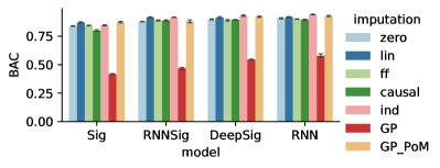
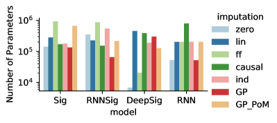
(a) PenDigits-R

(b) PenDigits-L

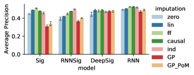
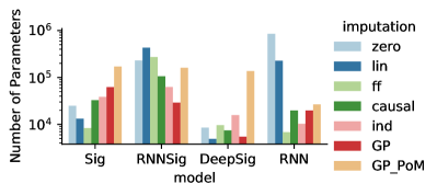
(c) Physionet2012

Figure 5: Visualisations for PenDigits and Physionet . The rows indicate datasets and different subsampling schemes (R for Random, L for Label-based). The left column displays the performance metric which was optimzied for: balanced accuracy (BAC), or average precision. The right column indicates the number of trainable parameters which the best model required (as selected in the hyperparameter search).

A.2 Imputation strategies

We consider the following set of strategies for path imputation, i.e.

1. linear interpolation: At a given imputation point, the previous and next observed data point are linearly interpolated. Missing values at the start or end of the time series are imputed with $0$ which for standardised data also corresponds to the mean.

2. forward filling: At a given imputation point, the last observed value is carried forward. Missing values at the start of the time series are imputed with $0$.

3. indicator imputation: At a given imputation point, for each feature dimension, if no observation is available a binary missingness indicator variable is set to $1$, $0$ otherwise. The missing value is filled with $0$.

4. zero imputation: At a given imputation point, missing values are filled with $0$.

5. causal imputation: This approach is related to forward filling and motivated by signature theory. As opposed to forward filling, the time and the actual value are updated sequentially. For more details, we introduce causal imputation in Section A.6.

6. Gaussian process adapter: We introduce GP adapters in Section 3, where $\mathbf{z}$ refers to the imputed time series (modelled as Gaussian distribution).

A.3 Dataset statistics and filtering

Physionet2012

As our focus is time series classification, for Physionet2012 [19], we included the 36 time series variables, and excluded the static covariates (notably, we counted the variable ‘weight’ as a static covariate). Subsequently, we excluded the following $12$ icu stays (here represented by there ids) for having no time series data (but only static covariates): $140501,150649,140936,143656,141264,145611,142998,147514,$ $142731,150309,155655,156254$, and a single noisy encounter, $135365$, which contained much more observations than all other patients. After these filtering steps, we count $11987$ instances and a binary class label, whether a patient survives the hospital stay or not.

PenDigits

For PenDigits [11], we count $10992$ samples, featuring $2$ channels and $8$ time steps, and $10$ classes.

LSST

LSST [1] contains $4925$ instances featuring $6$ channel dimensions and $36$ time steps. This dataset contains $14$ classes.

CharacterTrajectories

This dataset contains $2858$ instances, featuring $3$ channel dimensions, $182$ time steps and $20$ classes [11].

A.4 Model implementations, architectures and hyperparameters

All models are implemented in Pytorch [36], whereas the GP adapter and GP-PoM are implemented using the GPyTorch framework [17]. Next, we specify the details of the model architectures.

Sig

We use a simple signature model that involves one signature block comprising of a linear augmentation followed by the signature transform. Subsequently, a final module of dense layers $(30,30)$ is used. This is architecture refers to the Neural-signature-augment model [3].

RNNSig

This model extends the signature transform to a window-based stream of signatures, where the final neural module is a GRU sliding over the stream of signatures. We allowed window sizes between $3$ and $10$ steps. For the GRU cell, we allowed any of the following number of hidden units: $[16,32,64,128]$.

RNN

Here, we use a standard RNN model using GRU cells. The size of hidden units was chosen as one of the following: $[16,32,64,128,256,512]$.

DeepSig

For the deep signature model we employ two signature blocks (each comprising a linear augmentation and the signature calculation) following Bonnier et al., [3].

A.4.1 Hyperparameters

For all signature-based models, we allowed a signature truncation depth of $2$–$4$, as we observed that larger values quickly led to a parameter explosion. All models were optimised using Adam [24]. Both the learning rates and weight decay were drawn log-uniformly between $10^{-4}$ and $10^{-2}$. We allowed for the following batch-sizes: $(32,64,128,256)$. For GP-based models, to save memory, we used virtual batching based on a batch-size of $32$. Furthermore, for standard GP adapters we used $10$ MC samples, conforming with recent literature [16, 33]. All approaches were constrained to have no more than $1.5$ million trainable parameters.

A.5 Fragile dependence on sampling in unrelated channels: example

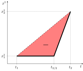
Figure 7: Lévy area of the forward-fill imputed path. By changing $t_{3/2}$ (a single unrelated observation!), we can make this disparity greater or smaller.

Suppose that we have observed the (very short) time series

$$\mathbf{x}=((t_{1},x_{1}^{1},x_{1}^{2}),(t_{2},x_{2}^{1},*))\in\mathcal{S}(\mathbb{R}^{2}).$$ (11)

Perhaps we now apply, say, forward fill data-imputation, to produce

$$((t_{1},x_{1}^{1},x_{1}^{2}),(t_{2},x_{2}^{1},x_{1}^{2})).$$

Finally we linearly path-impute to create the linear path

$$f \colon[t_{1},t_{2}]\to\mathbb{R}\times\mathbb{R}^{2}$$

$$f \colon t\mapsto\left(t,x_{1}^{1}\frac{t_{2}-t}{t_{2}-t_{1}}+x_{2}^{1}\frac{t-t_{1}}{t_{2}-t_{1}},x_{1}^{2}\right),$$

to which we may then apply the signature transform. In particular we will have computed the Lévy area with respect to $t$ and $x^{1}$. As this is just a straight line, the Lévy area is zero.

Now suppose we include an additional observation at some time $t_{3/2}\in(t_{1},t_{2})$, so that our data is instead

$$\mathbf{x}=((t_{1},x_{1}^{1},x_{1}^{2}),(t_{3/2},*,x_{3/2}^{2}),(t_{2},x_{2}^{1},*)).$$ (12)

Then the same procedure as before will produce the data

$$\mathbf{x}=((t_{1},x_{1}^{1},x_{1}^{2}),(t_{3/2},x_{1}^{1},x_{3/2}^{2}),(t_{2},x_{2}^{1},x_{3/2}^{2})),$$

with corresponding function $f$. The $(t,x^{1})$ components of $f$ and its $(t,x^{1})$-Lévy area are shown in Figure 7. As a result of an unrelated observation in the $x^{2}$ channel, the $(t,x^{1})$-Lévy area has been changed. The closer $t_{3/2}$ is to $t_{2}$, the greater the disparity. This simple example underscores the danger of ‘just forward-fill data-imputing’. Doing so has introduced an undesired dependency on the simple presence of an observation in other channels, with the change in our imputed path being determined by the time at which this other observation occurred.

Indeed, any imputation scheme that predicts something other than the unique value lying on the dashed line in Figure 7, will fail. This means that this example holds for essentially every data-imputation scheme—the only scheme that survives this flaw is the linear data-imputation scheme. This is the unique imputation scheme that coincides with the linear path-imputation that must be our concluding step. However, when there is missing data at the start or the end of a partially observed times series, then there is no ‘next observation’ which linear imputation may use. So in general, we cannot uniformly apply the linear data-imputation scheme, and must choose another scheme or find ad-hoc solutions for missing data at the start or the end of the time series. Furthermore, it is plausible to assume that linear interpolation suffers from low expressivity as an imputation scheme which might empirically mask this benefit.

A.6 Causal signature imputation

In Section A.5 we have spoken about the limitations of traditional data-imputation schemes, and at first glance one may be forgiven for thinking that these are issues are unavoidable. However, it turns out that we need not be limited just to these traditional imputation schemes. The trick is to consider time not as a parameterisation, but as a channel. This leads to a ‘meta imputation strategy’, which we refer to as causal signature imputation. It will turn any traditional causal data-imputation strategy (for example, feed-forward) into a causal path-imputation strategy for signatures; at the same time it will overcome the issue of a fragile dependence.

Suppose we have $\mathbf{x}\in\mathcal{S}(\mathcal{X}^{*})$, and some favourite choice of causal data-imputation strategy $c\colon\mathcal{S}(\mathcal{X}^{*})\to\mathcal{S}(\mathcal{X})$. Next, given

$$\mathbf{x}=((t_{1},x_{1}),\ldots,(t_{n},x_{n}))\in\mathcal{S}(\mathcal{X}),$$ (13)

we define the operation $\Omega\colon\mathcal{S}(\mathcal{X})\to\mathcal{S}(\mathcal{X})$ by

$$\Omega(\mathbf{x})=( (t_{1},x_{1}),(t_{2},x_{1}),(t_{2},x_{2}),(t_{3},x_{2}),$$

$$\ldots,$$

$$(t_{i},x_{i}),(t_{i+1},x_{i}),(t_{i+1},x_{i+1}),(t_{i+2},x_{i+1}),$$

$$\ldots,$$

$$(t_{n-1},x_{n-1}),(t_{n},x_{n-1}),(t_{n},x_{n})).$$ (14)

That is, first time is updated, and then the corresponding observation in data space is updated. This means that the change in data space occurs instantaneously.

For each $n\in\mathbb{N}$ (and given $a<b$), fix any $s_{i}^{(n)}$ for $i\in\{1,\ldots,n\}$. (We will see that the exact choice is unimportant in a moment.) Given

$$\mathbf{x}=((t_{1},x_{1}),\ldots,(t_{n},x_{n}))\in\mathcal{S}(\mathcal{X}),$$

let $\psi\colon\mathcal{S}(\mathcal{X})\to(\mathbb{R}\times\mathcal{X})^{[a,b]}$ be the unique continuous piecewise linear path such that $\psi(s_{i}^{(n)})=(t_{i},x_{i})$. Note that this is just a slight generalisation of the linear path-imputation that has already been performed so far; we are simply no longer asking for additional assumptions of the form $s_{i}^{(n)}=t_{i}$.

Finally, we put this all together, and define the causal signature imputation strategy $\phi_{c}$ associated with $c$ to be

$$\phi_{c}=\psi\circ\Omega\circ c,$$

which will be a map $\mathcal{S}(\mathcal{X}^{*})\to(\mathbb{R}\times\mathcal{X})^{[a,b]}$. Thus $\phi_{c}$ defines a family of path-imputation schemes, parameterised by a choice of data-imputation scheme.

Before we analyse why this works in practice, we repeat a crucial property of the signature transform [3, Appendix A].

Theorem 1 (Invariance to reparameterisation).

Let $f\colon[a,b]\to\mathbb{R}^{d}$ be a continuous piecewise differentiable path. Let $\psi\colon[a,b]\to[c,d]$ be continuously differentiable, increasing, and surjective. Then $\mathrm{Sig}^{N}(f)=\mathrm{Sig}^{N}(f\circ\psi)$.

Coming back to our analysis, we first note that the previous theorem implies that the signature transform of $\phi_{c}(\mathbf{x})$ is invariant to the choice of $s_{i}^{(n)}$. Second, note that holding time between observations fixed is a valid choice, by the definition for $\mathcal{S}$ in equation (2). There should hopefully be no moral objection to our definition of $\mathcal{S}$, as holding time fixed essentially just corresponds to a jump discontinuity; not such a strange thing to have occur. Here, by replacing time as the parameterisation, we are then able to recover the continuity of the path. Third, we claim that $\phi_{c}$ is immune to the two major flaws of imputation methods, namely (i) their fragile dependence on sampling in unrelated channels, and (ii) their non-causality. Let us consider the first flaw of dependence on sampling in unrelated channels. For simplicity, take $c$ to be the forward-fill data-imputation strategy. Consider again the $\mathbf{x}$ defined in expression (11). This means that

$$\phi_{c}(\mathbf{x})=\psi(\;((t_{1},x_{1}^{1},x_{1}^{2}),(t_{2},x_{1}^{1},x_{1}^{2}),(t_{2},x_{2}^{1},x_{1}^{2}))\;).$$ (15)

Contrast adding in the extra observation at $t_{3/2}$ as in equation (12). Then

$$\phi_{c}(\mathbf{x})(s)$$

$$=\psi(\;((t_{1},x_{1}^{1},x_{1}^{2}),(t_{3/2},x_{1}^{1},x_{1}^{2}),(t_{3/2},x_{1}^{1},x_{3/2}^{2}),$$

$$\hskip 31.0001pt(t_{2},x_{1}^{1},x_{3/2}^{2}),(t_{2},x_{2}^{1},x_{3/2}^{2}))\;).$$ (16)

Evaluating each $\psi$ will then in each case give a path with three channels, corresponding to $t,x^{1},x^{2}$. Then it is clear that the $(t,x^{1})$ component of the path in equation (15) is just a reparameterisation of the path in equation (16), a difference which is irrelevant by Theorem 1. (And the $x^{2}$ component of the second path has been updated to use the new information $x_{3/2}^{2}$.) Thus the causal path impuation scheme is robust to such issues. For general time series and $c$ taken to be any other causal data-imputation strategy, then much the same analysis can be easily be performed.

Now consider the second potential flaw, of non-causality. The issue previously arose because of the non-causality of the linear path-imputation. We see from equation (14), however, such changes only occur in data space while the time channel is frozen; conversely the time channel only updates with the value in the data space frozen. Provided that $c$ is also causal, then causality will, overall, have been preserved. For example, it is possible to use this scheme in an online setting. There are interesting comparisons to be made between causal signature imputation and certain operations in the signature literature. First is the lead-lag transform [8]. With the lead-lag transform, the entire path is duplicated, and then each side is alternately updated. Conversely, in causal signature imputation, the path is instead split between $t$ and $(x^{1},\ldots,x^{n})$, and then each side is alternately updated. Second is the comparison to the linear and rectilinear embedding strategies, see for example [12]. It is possible to interpret $\psi\circ\Phi$ as a hybrid between the linear and rectilinear embeddings: it is rectilinear with respect to an ordering of $t$ and $(x^{1},\ldots,x^{n})$, and linear on $(x^{1},\ldots,x^{n})$. Furthermore, the time-joined transformation [27] is pursuing a very similar goal to the here described causal signature imputation. This is also why we do not consider this imputation strategy as a novel contribution of this work.

A.6.1 Comparison to the Fourier and wavelet transforms

The signature transform exhibits a certain similarity to the one-dimensional Fourier or wavelet transforms. Both are integrals of paths. However, in reality these transforms are fundamentally different. Both the Fourier and wavelet transforms are linear transforms, and operate on each channel of the input path separately. In doing so they model the path as a linear combination of elements from some basis.

Conversely, the signature transform is a nonlinear transform - indeed, it is a universal nonlinearity - and operates by combining information between different channels of the input path. In doing, the signature transform models functions of the path; the universal nonlinearity property says that in some sense it provides a basis for such functions.

References

- Allam Jr et al., [2018] Allam Jr, T., Bahmanyar, A., Biswas, R., Dai, M., Galbany, L., Hložek, R., Ishida, E. E., Jha, S. W., Jones, D. O., Kessler, R., et al. (2018). The photometric lsst astronomical time-series classification challenge (plasticc): Data set. arXiv preprint arXiv:1810.00001.
- Bailer-Jones et al., [1998] Bailer-Jones, C., MacKay, D., and Withers, P. (1998). A recurrent neural network for modelling dynamical systems. Network: Computation in Neural Systems, 9:531–47.
- Bonnier et al., [2019] Bonnier, P., Kidger, P., Perez Arribas, I., Salvi, C., and Lyons, T. (2019). Deep Signature Transforms. In Advances in Neural Information Processing Systems, pages 3099–3109.
- Che et al., [2018] Che, Z., Purushotham, S., Cho, K., Sontag, D., and Liu, Y. (2018). Recurrent neural networks for multivariate time series with missing values. Scientific reports, 8(1):1–12.
- Chen, [1954] Chen, K. T. (1954). Iterated integrals and exponential homomorphisms. Proc. London Math. Soc, 4, 502–512.
- Chen, [1957] Chen, K. T. (1957). Integration of paths, geometric invariants and a generalized Baker-Hausdorff formula. Ann. of Math. (2), 65:163–178.
- Chen, [1958] Chen, K. T. (1958). Integration of paths - a faithful representation of paths by non-commutative formal power series. Trans. Amer. Math. Soc. 89 (1958), 395–407.
- Chevyrev and Kormilitzin, [2016] Chevyrev, I. and Kormilitzin, A. (2016). A primer on the signature method in machine learning. arXiv:1603.03788.
- Chevyrev and Oberhauser, [2018] Chevyrev, I. and Oberhauser, H. (2018). Signature moments to characterize laws of stochastic processes. arXiv:1810.10971.
- Cho et al., [2014] Cho, K., Van Merriënboer, B., Gulcehre, C., Bahdanau, D., Bougares, F., Schwenk, H., and Bengio, Y. (2014). Learning phrase representations using RNN encoder-decoder for statistical machine translation. arXiv:1406.1078.
- Dua and Graff, [2017] Dua, D. and Graff, C. (2017). UCI machine learning repository.
- Fermanian, [2019] Fermanian, A. (2019). Embedding and learning with signatures. arXiv:1911.13211.
- Fey et al., [2018] Fey, M., Eric Lenssen, J., Weichert, F., and Müller, H. (2018). SplineCNN: Fast Geometric Deep Learning With Continuous B-Spline Kernels. In The IEEE Conference on Computer Vision and Pattern Recognition (CVPR).
- Friz and Victoir, [2010] Friz, P. K. and Victoir, N. B. (2010). Multidimensional stochastic processes as rough paths: theory and applications. Cambridge University Press.
- Funahashi and Nakamura, [1993] Funahashi, K.-i. and Nakamura, Y. (1993). Approximation of dynamical systems by continuous time recurrent neural networks. Neural Networks, 6(6):801 – 806.
- Futoma et al., [2017] Futoma, J., Hariharan, S., and Heller, K. (2017). Learning to Detect Sepsis with a Multitask Gaussian Process RNN Classifier. In Proceedings of the 34th International Conference on Machine Learning, pages 1174–1182.
- Gardner et al., [2018] Gardner, J., Pleiss, G., Weinberger, K. Q., Bindel, D., and Wilson, A. G. (2018). GPyTorch: Blackbox matrix-matrix Gaussian Process inference with GPU acceleration. In Advances in Neural Information Processing Systems 31, pages 7576–7586.
- Gelman and Hill, [2007] Gelman, A. and Hill, J. (2007). Data Analysis Using Regression and Multilevel/Hierarchical Models. Cambridge University Press.
- Goldberger et al., [2000] Goldberger, A. L., Amaral, L. A., Glass, L., Hausdorff, J. M., Ivanov, P. C., Mark, R. G., Mietus, J. E., Moody, G. B., Peng, C.-K., and Stanley, H. E. (2000). Physiobank, physiotoolkit, and physionet: components of a new research resource for complex physiologic signals. circulation, 101(23):e215–e220.
- Hambly and Lyons, [2010] Hambly, B. M. and Lyons, T. J. (2010). Uniqueness for the signature of a path of bounded variation and the reduced path group. Annals of Mathematics, 171(1):109–167.
- Horn et al., [2019] Horn, M., Moor, M., Bock, C., Rieck, B., and Borgwardt, K. (2019). Set functions for time series. arXiv preprint arXiv:1909.12064.
- Kidger and Lyons, [2020] Kidger, P. and Lyons, T. (2020). Signatory: differentiable computations of the signature and logsignature transforms, on both CPU and GPU. arXiv:2001.00706. https://github.com/patrick-kidger/signatory.
- Kidger et al., [2020] Kidger, P., Morrill, J., Foster, J., and Lyons, T. (2020). Neural Controlled Differential Equations for Irregular Time Series. arXiv:2005.08926.
- Kingma and Ba, [2014] Kingma, D. P. and Ba, J. (2014). Adam: A method for stochastic optimization. arXiv preprint arXiv:1412.6980.
- Király and Oberhauser, [2019] Király, F. J. and Oberhauser, H. (2019). Kernels for sequentially ordered data. Journal of Machine Learning Research.
- Kormilitzin et al., [2016] Kormilitzin, A. B., Saunders, K. E. A., Harrison, P. J., Geddes, J. R., and Lyons, T. J. (2016). Application of the signature method to pattern recognition in the cequel clinical trial. arXiv:1606.02074.
- Levin et al., [2013] Levin, D., Lyons, T., and Ni, H. (2013). Learning from the past, predicting the statistics for the future, learning an evolving system. arXiv:1309.0260.
- Li et al., [2017] Li, C., Zhang, X., and Jin, L. (2017). LPSNet: a novel log path signature feature based hand gesture recognition framework. In Proceedings of the IEEE International Conference on Computer Vision, pages 631–639.
- Li and Marlin, [2016] Li, S. C.-X. and Marlin, B. M. (2016). A scalable end-to-end Gaussian process adapter for irregularly sampled time series classification. In Advances in Neural Information Processing Systems, pages 1804–1812.
- Liao et al., [2019] Liao, S., Lyons, T., Yang, W., and Ni, H. (2019). Learning stochastic differential equations using rnn with log signature features. arXiv:1908.08286.
- Lyons, [2014] Lyons, T. (2014). Rough paths, signatures and the modelling of functions on streams. arXiv:1405.4537.
- Lyons, [1998] Lyons, T. J. (1998). Differential equations driven by rough signals. Revista Matemática Iberoamericana, 14(2):215–310.
- Moor et al., [2019] Moor, M., Horn, M., Rieck, B., Roqueiro, D., and Borgwardt, K. (2019). Early recognition of sepsis with gaussian process temporal convolutional networks and dynamic time warping. In Machine Learning for Healthcare Conference, pages 2–26.
- [34] Morrill, J., Kormilitzin, A., Nevado-Holgado, A., Swaminathan, S., Howison, S., and Lyons, T. (2019a). The signature-based model for early detection of sepsis from electronic health records in the intensive care unit. In 2019 Computing in Cardiology (CinC), pages Page–1. IEEE.
- [35] Morrill, J., Kormilitzin, A., Nevado-Holgado, A., Swaminathan, S., Howison, S., and Lyons, T. (2019b). The Signature-based Model for Early Detection of Sepsis from Electronic Health Records in the Intensive Care Unit. International Conference in Computing in Cardiology.
- Paszke et al., [2019] Paszke, A., Gross, S., Massa, F., Lerer, A., Bradbury, J., Chanan, G., Killeen, T., Lin, Z., Gimelshein, N., Antiga, L., Desmaison, A., Kopf, A., Yang, E., DeVito, Z., Raison, M., Tejani, A., Chilamkurthy, S., Steiner, B., Fang, L., Bai, J., and Chintala, S. (2019). Pytorch: An imperative style, high-performance deep learning library. In Advances in Neural Information Processing Systems 32, pages 8024–8035.
- Perez Arribas et al., [2018] Perez Arribas, I., Goodwin, G. M., Geddes, J. R., Lyons, T., and Saunders, K. E. A. (2018). A signature-based machine learning model for distinguishing bipolar disorder and borderline personality disorder. Translational Psychiatry, 8(1):274.
- Reizenstein, [2019] Reizenstein, J. (2019). Iterated-integral signatures in machine learning. PhD thesis, University of Warwick. http://wrap.warwick.ac.uk/131162/.
- Reizenstein and Graham, [2018] Reizenstein, J. and Graham, B. (2018). The iisignature library: efficient calculation of iterated-integral signatures and log signatures. arXiv:1802.08252.
- Reyna et al., [2019] Reyna, M. A., Josef, C. S., Jeter, R., Shashikumar, S. P., Westover, M. B., Nemati, S., Clifford, G. D., and Sharma, A. (2019). Early prediction of sepsis from clinical data: the physionet/computing in cardiology challenge 2019. Critical Care Medicine.
- Rubanova et al., [2019] Rubanova, Y., Chen, T. Q., and Duvenaud, D. K. (2019). Latent ordinary differential equations for irregularly-sampled time series. In Advances in Neural Information Processing Systems, pages 5321–5331.
- Rubin, [1976] Rubin, D. B. (1976). Inference and missing data. Biometrika, 63(3):581–592.
- Shukla and Marlin, [2019] Shukla, S. N. and Marlin, B. (2019). Interpolation-prediction networks for irregularly sampled time series. In International Conference on Learning Representations.
- Toth and Oberhauser, [2019] Toth, C. and Oberhauser, H. (2019). Variational Gaussian Processes with Signature Covariances. arXiv:1906.08215.
- Yang et al., [2016] Yang, W., Jin, L., Ni, H., and Lyons, T. (2016). Rotation-free online handwritten character recognition using dyadic path signature features, hanging normalization, and deep neural network. In 2016 23rd International Conference on Pattern Recognition (ICPR), pages 4083–4088. IEEE.
- Yang et al., [2017] Yang, W., Lyons, T., Ni, H., Schmid, C., Jin, L., and Chang, J. (2017). Leveraging the path signature for skeleton-based human action recognition. arXiv:1707.03993.