The Techni-Pati-Salam Composite Higgs

Abstract

Composite Higgs models can be extended to the Planck scale by means of the partially unified partial compositeness (PUPC) framework. We present in detail the Techni-Pati-Salam model, based on a renormalizable gauge theory $SU(8)_{PS}\times SU(2)_{L}\times SU(2)_{R}$. We demonstrate that masses and mixings for all generations of standard model fermions can be obtained via partial compositeness at low energy, with four-fermion operators mediated by either heavy gauge bosons or scalars. The strong dynamics is predicted to be that of a confining $Sp(4)_{\rm HC}$ gauge group, with hyper-fermions in the fundamental and two-index anti-symmetric representations, with fixed multiplicities. This motivates for Lattice studies of the Infra-Red near-conformal walking phase, with results that may validate or rule out the model. This is the first complete and realistic attempt at providing an Ultra-Violet completion for composite Higgs models with top partial compositeness. In the baryon-number conserving vacuum, the theory also predicts a Dark Matter candidate, with mass in the few TeV range, protected by semi-integer baryon number.

I Introduction

The Standard Model (SM) of particle physics Glashow:1961tr ; Weinberg:1967tq ; Salam:1968rm has withstood all the attempts at discovering signs of New Physics, with most recently the null results from the LHC experiments. The discovery of a Higgs-like boson Aad:2012tfa ; Chatrchyan:2012xdj has further confirmed the validity of the SM. The main experimental confirmation has come from precise measurements in the electroweak (EW) sector of the theory, with most prominent results coming from LEP Barbieri:2004qk . What we know with a precision at the level of per-mille, is that there exist three Goldstone bosons, i.e. the longitudinal polarizations of the $W^{\pm}$ and $Z$ gauge bosons, that complement the gauge principle in the SM and provide mass to the weak gauge bosons Englert:1964et ; Higgs:1964ia ; Higgs:1964pj ; Guralnik:1964eu . While all experimental results seem to point towards a SM-like Higgs boson, our knowledge of its properties is still far from the precision achieved in the gauge sector: the couplings of the Higgs boson are only known at best at the level of $10\%$ Khachatryan:2016vau , and the precision will not improve greatly at the end of the LHC programme Cepeda:2019klc . This experimental status leaves open the question of the true nature of the discovered Higgs boson.

On the model building side, the SM lacks two key ingredients that play a crucial role in our understanding of our Universe: gravitational interactions and a Dark Matter candidate. This simple observation points towards the existence of a new physical scale, ultimately the Planck mass from gravity, thus keeping open the long standing hierarchy problem between the EW scale and such Ultra-Violet (UV) scale. The presence of an elementary scalar field in the Higgs sector is particularly at odds with the observed hierarchy, as a scalar mass receives quantum corrections proportional to the new physical scale. The discovery of a Higgs boson with a mass of $125$ GeV can, therefore, be considered a materialization of the so-called “naturalness” problem. A time-honored possibility Weinberg:1975gm is to replace the elementary Higgs sector of the SM with a strong confining dynamics: the EW scale would therefore be generated dynamically, like the QCD scale, and the EW symmetry breaking (EWSB) can be ascribed to a spontaneous chiral symmetry breaking. While the first proposals were essentially Higgless Dimopoulos:1979es ; Eichten:1979ah , it was soon realized that extending the global symmetry of the theory allows the entire Higgs doublet to arise as a pseudo-Nambu-Goldstone boson (pNGB) of the condensing strong sector Kaplan:1983fs . This new approach kills two birds with one stone: it explains why the Higgs boson is lighter than other composite states (in agreement with the null results of New Physics searches at the LHC) and the ten per-cent agreement of the composite Higgs couplings to SM predictions, at the price of generating a “little hierarchy” Barbieri:2000gf between the EW scale $v=246$ GeV and the compositeness scale. The latter is encoded in the pNGB decay constant $f\approx\mathcal{O}(1)$ TeV.

The nemesis of this approach to the EWSB is the generation of fermion masses Dimopoulos:1979es ; Eichten:1979ah : as SM fermion couplings to the strong sector typically arise via higher dimension operators, generating large masses (i.e., the top mass) is generically at odds with fulfilling constraints from flavor changing neutral currents (FCNCs). Many palliatives have been proposed: among the most remarkable are the presence of an Infra-Red (IR) conformal phase Holdom:1981rm and the mechanism of fermion Partial Compositeness (PC) Kaplan:1991dc . The former relies on the property that the strong sector enters a “walking” phase Cohen:1988sq right above the condensation scale, where a large anomalous dimension of the composite Higgs operator is generated, allowing to push the flavor scale high enough without suppressing the SM fermion mass operators. In the latter, Yukawa-like couplings are replaced by linear mixing of the SM fermion fields to fermionic composite operators, in such a way that the large anomalous dimensions are associated to composite baryonic operators instead of the Higgs one. This scenario has been revived in the early 2000’s thanks to the principle of holography Contino:2003ve , which allowed to relate a composite pNGB Higgs in a nearly-conformal theory to a gauge boson in a warped five-dimensional theory. Composite Higgs models thus merged with Gauge-Higgs unification model building in warped space Hosotani:2005nz , leading to the definition of a minimal model based on the symmetry breaking SO(5)/SO(4) Agashe:2004rs ; Agashe:2005dk , where only the Higgs doublet populates the pNGB sector of the theory. A lot of work has been devoted in the literature on this scenario, and we refer to the recent reviews Contino:2010rs ; Bellazzini:2014yua ; Panico:2015jxa ; Cacciapaglia:2020kgq and references therein. Yet, most of the results in the literature rely on effective field theory (EFT) analyses, both for studying the phenomenology and for developing various model building aspects of the composite Higgs paradigm. In the case of the flavor issue Matsedonskyi:2014iha ; Cacciapaglia:2015dsa ; Panico:2016ull , for instance, it has been found that light top partners are allowed as soon as flavor structures for light generations can be generated at a higher scale separated from the condensation scale by a near-conformal phase.

In this article, we want to face the daring need for an UV completion for composite Higgs models: this step is crucial in order to base all we learned from EFT studies on more solid foundations and to truly understand the origin of flavor physics. Following the holography principle, one may be tempted to invoke extra dimensional theories as genuine UV completions Agashe:2005vg . We do not find this route satisfactory. On the one hand, some basic requirements at the foundation of the original holographic conjecture Maldacena:1997re , like the presence of maximal supersymmetry, are not satisfied in the minimal models studied so far. Holography applied outside of supersymmetry and string theory, while proven to be phenomenologically useful even in QCD Erlich:2005qh ; DaRold:2005mxj ; Hirn:2005nr , is less robust and tested that the original one, mainly due to the lack of calculability in the strongly-coupled side. Example of models based on more solid supersymmetric dualities can be found in Refs Caracciolo:2012je ; Marzocca:2013fza , however these theories lack a complete theory of flavor. On the other hand, it is not clear at all if extra dimensional theories are fundamental because of the mass dimension carried by gauge couplings themselves Gies:2003ic ; Morris:2004mg . An attractive and time-honored route is offered by microscopic gauge-fermion theories, similar to QCD for mesons and hadrons, defined in terms of a renormalizable and fundamental 4-dimensional gauge theory (we refer the reader to the recent review of this approach in Cacciapaglia:2020kgq ). Attempts to build microscopic descriptions of theories of top PC can be found in Refs Barnard:2013zea ; Ferretti:2013kya ; Vecchi:2015fma : these analyses lead to the interesting conclusion that there exists a limited number of theories apt at describing the low energy composite spectrum Ferretti:2016upr ; Belyaev:2016ftv . These models, however, are not genuine UV completions: they are only able to characterize the dynamics of the model below the condensation scale, where resonances associated to the pNGB Higgs and top PC are needed. Crucial ingredients like the near conformal dynamics, the origin of the PC couplings and the masses for leptons and light quarks are absent. The theories are in fact defined in such a way that they are outside of the conformal window, i.e. they do condense at low energy. Lattice studies of some of these theories are also available DeGrand:2015zxa ; Bennett:2017kga ; Ayyar:2018zuk ; Ayyar:2018glg ; Bennett:2019jzz ; Hasenfratz:2016gut . An alternative way to UV complete fermion PC is to introduce (light) scalar fields charged under the confining gauge symmetry Sannino:2016sfx ; Cacciapaglia:2017cdi : at the price of giving up naturalness, one potentially obtains a complete and fundamental theory of flavor Sannino:2017utc . We should also mention the possibility of bosonic Technicolor Samuel:1990dq , where an elementary Higgs doublet is re-introduced Galloway:2016fuo ; Agugliaro:2016clv . Trying to achieve a complete theory based on gauge and fermion fields is a much more daring task: this would be similar to the quest for extended Technicolor theories Dimopoulos:1979es ; Eichten:1979ah that, despite intense efforts Hill:2002ap ; Appelquist:2003uu ; Appelquist:2003hn ; Appelquist:2004ai , has not produced any fully realistic model so far. In Ref. Cacciapaglia:2019vce an attempt has been made to achieve top PC in confining chiral gauge theories. More recently, large $N_{f}$ asymptotic safety Antipin:2017ebo has been proposed as a route to the Planck scale for gauge-fermion top PC models Cacciapaglia:2018avr , yet the four fermion interactions leading to PC need to be generated by mediation of heavy scalars.

In the present work, we follow the route opened in Ref. Cacciapaglia:2019dsq within the partially unified partial compositeness (PUPC) framework: the confining gauge symmetry is partially unified with the SM ones, with the gauge symmetry breaking due to high-scale scalars. In this sense, this approach lies in between the early extended Technicolor approaches and theories with scalars, while retaining the ambition of achieving a complete theory of flavor in a natural way, i.e. without large hierarchies between scalar masses and the Planck scale. The partial compositeness four-fermion (PC4F) interactions are thus mediated by the massive gauge bosons, as well as by the heavy scalars, with large anomalous dimensions still needed to achieve unsuppressed low energy operators in the condensed phase Contino:2010rs . While it is hard to produce accurate low energy predictions, mainly due to the presence of strong coupling regimes in the IR walking phase and at low energies, we want to demonstrate in detail how a complete theory of flavor can be achieved in this framework. While the general idea is described in Ref. Cacciapaglia:2019dsq , here we focus specifically on the Techni-Pati-Salam (TPS) model based on a partially unified gauge symmetry

$$\mathcal{G}_{\rm TPS}=SU(8)_{\rm PS}\times SU(2)_{L}\times SU(2)_{R}\,.$$

We will show how to construct a minimal model, which also helps predicting the properties of the microscopic theory underlying the low energy composite dynamics (that can be studied on the lattice), and the dynamics of the walking phase. Analysing how flavor structures arise can help better understand the low energy properties of composite models: for instance, we can show that the multi-scale scenario of Ref. Panico:2016ull cannot be achieved in this framework and only top partners, i.e. light-ish spin-1/2 resonances associated to the third generation, are possible.

The article is organised as follows. In Section II we present the general features of the PUPC framework, and the characteristics that lead us to focus on the TPS model and its symmetry breaking pattern. In Section III we discuss in detail how the masses for the third generation of SM fermions can be generated, starting from a fundamental gauge-Yukawa theory at high scale. In particular, we will show how the mass hierarchy between top, bottom, tau and neutrino can be achieved. In Section IV we investigate the possibility of extending the construction to the first and second families: we identify the necessary and minimal ingredients needed to generating all masses and non-trivial Cabibbo-Kobayashi-Maskawa (CKM) Cabibbo:1963yz ; Kobayashi:1973fv and Pontecorvo-Maki-Nakagawa-Sakata (PMNS) Maki:1962mu mixing matrices. We also establish how baryon number conservation can be imposed to avoid proton decay, thus leading to the existence of a potential Dark Matter candidate. We offer our conclusion and the perspectives in Section V.

II General considerations

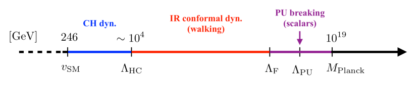
Figure 1: Schematic representation of the dynamical phases of PUPC models.

The main goal of our PUPC approach Cacciapaglia:2019dsq is to provide a genuine UV completion for composite Higgs models with top partial compositeness, which could explain the origin of the partial compositeness couplings and flavor physics. The theory also needs to be valid all the way up to the Planck scale, where quantum gravity effects become relevant. To achieve this goal, we require that the theory in the UV consists of a renormalizable gauge-Yukawa theory. Scalars, therefore, are added with a “natural” potential, in the sense that all the dimension-of-mass parameters are not too far from the Planck scale. We remind the reader that this “naturalness” principle does not apply to fermion masses. The low energy target is a composite Higgs model with, at least, top partial compositeness. This implies that the UV theory needs to provide both the couplings to achieve top PC, and an intermediate walking phase to enhance them at low energy: the PUPC model, therefore, needs to pass through several different dynamical phases at various scales, as schematically depicted in Fig. 1. Here, we expect the low energy dynamics, above the EW scale, to be that of a confining theory with a typical scale $\Lambda_{\rm HC}\approx 10$ TeV (implying a Higgs pNGB decay constant $f\approx\frac{\Lambda_{\rm HC}}{4\pi}\approx 1$ TeV). An IR walking phase thus occurs, separating the confinement scale from the scale where flavor physics is generated, $\Lambda_{\rm F}$. How large this scale needs to be depends on the flavor bounds in a specific model, however we expect it to be close to the scale of gauge symmetry breaking of the UV theory. The latter is achieved by giving vacuum expectation values (VEVs) to the scalars in the theory, at a scale $\Lambda_{\rm PU}$, which is allowed to be roughly one loop-factor below $M_{\rm Planck}$. Thus, typically, $\Lambda_{\rm F}\approx\Lambda_{\rm PU}\approx 10^{16\div 19}$ GeV.

In this section, we will present some general features of PUPC models. The first issue is about choosing the gauge groups. Then, we will show how the SM fermions can be embedded into the PUPC theory, and the scalar sector needed for the symmetry breaking. Finally, we will discuss the conditions under which a walking dynamics can be achieved. In the following two sections we will discuss more gory details about the generation of masses for the third generation first, and then how to extend the theory to the light generations and full flavor structures.

We will start this exploration from the IR end of the spectrum. It has been shown that only a finite number of gauge-fermion theories can lead to the desired low energy phase Barnard:2013zea ; Ferretti:2013kya ; Vecchi:2015fma , where both a pNGB Higgs and top PC are achieved. The latter is due to the presence of light baryonic (spin-1/2) resonances with the SM quantum numbers matching the top field ones. These theories introduce a new gauge symmetry, called Hyper-Color (HC), with one or two representations for the new hyper-fermions. The strongest constraint on such models comes from the requirement that the gauge dynamics lies outside of the conformal window Dietrich:2006cm ; Sannino:2009aw ; Ryttov:2009yw ; Mojaza:2012zd , i.e. it condenses at low energies and breaks the chiral symmetries in the fermion sector. This requirements leaves only a handful of possibilities Ferretti:2016upr , as it is a strong constraint on the number of fermions and number of hyper-colors. Following the nomenclature of Ref. Belyaev:2016ftv , 12 minimal models have been identified, M1-M12, each characterized by its own gauge group and hyper-fermion representations. As mentioned, such theories lie outside of the conformal window: in order to enter the needed walking phase between $\Lambda_{\rm HC}$ and $\Lambda_{\rm F}$, additional hyper-fermions can be added, with a mass $\sim\Lambda_{\rm HC}$. This IR theory, then, needs to be embedded in the UV PUPC theory, where the HC gauge group is partially unified with the SM one. We will shortly see that this step is non-trivial, and it has consequences for the low energy dynamics, as it can be used to further select the gauge theories in the confined phase. This selection is crucial in particular for Lattice studies.

The models that achieve the low energy dynamics with top PC resort to HC groups $SO(N)_{\rm HC}$, $SU(N)_{\rm HC}$ and $Sp(N)_{\rm HC}$, with hyper-fermions in the fundamental, spinorial and two-index antisymmetric representations. Following minimality, we decided to unify QCD and HC groups: this is due to the fact that mediators for top PC typically carry QCD charges. As a consequence, we need to embed the hyper-fermion representation and $SU(3)_{c}$ fundamentals in the same representation of the extended-HC (EHC) group: this is easiest to do for models based on $Sp(N)_{\rm HC}$, like model M8 Barnard:2013zea ; Belyaev:2016ftv . The reason is that $SO(N)_{\rm HC}$ models always contain the spinorial representation, which is hard to embed together with a fundamental of QCD, while $SU(N)_{\rm HC}$ theories with fundamental tend to inherit the chiral spectrum of the SM in the hyper-fermion sector. While this analysis certainly does not exclude other possibilities, we decided for simplicity to focus on M8, as a template IR model for the first PUPC construction.

The low energy model, therefore, will consist on $Sp(4)_{\rm HC}$ with four hyper-fermions in the fundamental representation: one pair forms a doublet of the gauged $SU(2)_{L}$ while the other a doublet of the custodial $SU(2)_{R}$ (the hypercharge corresponds to the diagonal generator). This sector ensures that the pNGB Higgs arises at low energy, and its effect preserves the custodial relation between the $W$ and $Z$ masses. Furthermore, the model needs to include hyper-fermions in the two-index antisymmetric representation in order to obtain top partners in the form of hyper-baryons. The HC and QCD gauge groups are unified as diagonal-subgroups of a $SU(7)_{\rm EHC}$. It is then possible to show that quarks and hyper-fermions in the fundamental can be embedded in fundamentals of $SU(7)_{\rm EHC}$, by suitably choosing the charges under a $U(1)_{\rm E}$, in order to fit the correct hypercharges and cancel gauge anomalies. Leptons here remain as singlets of $SU(7)_{\rm EHC}$, thus they will not receive any contribution to their coupling to hyper-fermions from gauge mediation. This feature, plus the cancellation of anomalies, points towards a unification of quarks–hyper-fermions with leptons, à la Pati-Salam Pati:1974yy . Finally, the PUPC gauge group we choose to work with is

$$\mathcal{G}_{\rm TPS}=SU(8)_{\rm PS}\times SU(2)_{L}\times SU(2)_{R}\,,$$ (1)

from which the name of Techni-Pati-Salam (TPS) model Cacciapaglia:2019dsq . The next two questions involve the choices of fermions in the TPS model, which can accommodate for both the chiral SM fermions and the non-chiral hyper-fermions, as well as the choice of scalars, which are responsible for breaking the TPS group down to the SM plus HC gauge symmetries.

II.1 Fermion embedding

In the TPS model, both SM fermions and hyper-fermions need to be embedded into representations of the TPS group. As we will see, the multiplicity and quantum numbers for the hyper-fermions are determined by this choice, thus while we use M8 as a template model, the details of the IR dynamics will not necessarily be the same. To indicate the representations, we will use the following notations:

$$\{{\bf d_{\rm PS}},\ {\bf d}_{L},\ {\bf d}_{R}\}\Rightarrow\mathcal{G}_{\rm TPS}\,,$$ (2)

where ${\bf d}_{X}$ indicates the dimension of the representation under the TPS group $X$, while for the IR quantum numbers we omit the $SU(2)_{L}$ (as it remains unbroken all the way from the UV to the IR) and use

$$(d_{4},\ d_{3})_{Y}\Rightarrow(Sp(4)_{\rm HC},SU(3)_{c})_{U(1)_{Y}}\,.$$ (3)

Details on how the IR gauge groups are embedded in the TPS one in the UV will be presented in the next subsection.

Firstly, for the SM fermions we follow the hint from Pati-Salam Pati:1974yy and we embedded them in a fundamental, $\Omega$, and anti-fundamental, $\Upsilon$, of $SU(8)_{\rm PS}$, as follows:

$$\Omega=\{{\bf 8},\ {\bf 2},\ {\bf 1}\}=\begin{pmatrix}L\\ q_{L}\\ l_{L}\end{pmatrix}\,,$$ (4)

$$\Upsilon=\{{\bf\bar{8}},\ {\bf 1},\ {\bf 2}\}=\begin{pmatrix}U_{d}&D_{u}\\ d^{c}_{R}&u^{c}_{R}\\ e^{c}_{R}&\nu^{c}_{R}\end{pmatrix}\,;$$ (5)

where all spinors are left-handed Weyl, and the two columns in Eq. (5) explicitly show the two components of the $SU(2)_{R}$ doublet. The rows follow the $SU(8)_{\rm PS}$ structure, where we embed the IR gauge groups in the following block-diagonal form:

$$SU(8)_{PS}\Rightarrow\left(\begin{array}[]{c|c|c}Sp(4)_{\rm HC}&\phantom{\Big{(}}&\\ \cline{1-3}\cr\phantom{\Big{(}}&SU(3)_{c}&\\ \cline{1-3}\cr&&\phantom{\Big{(}xxx}\end{array}\right)\,.$$ (6)

One set of $\Omega$ and $\Upsilon$, therefore, contains a complete SM generation

$$\begin{array}[]{c}\phantom{\Big{(}}q_{L}=(1,3)_{1/6}\,,\;\;t_{R}^{c}=(1,\bar{3})_{-2/3}\,,\;\;b_{R}^{c}=(1,\bar{3})_{1/3}\,,\phantom{\Big{(}}\\ \phantom{\Big{(}}l_{L}=(1,1)_{-1/2}\,,\;\;e_{R}^{c}=(1,1)_{1}\,,\;\;\nu_{R}^{c}=(1,1)_{0}\,,\phantom{\Big{(}}\end{array}$$ (7)

including a right-handed neutrino, and the 4 hyper-fermions that generate the pNGB Higgs as a bound state (as in M8)

$$L=(4,1)_{0}\,,\;\;U_{d}=(4,1)_{1/2}\,,\;\;D_{u}=(4,1)_{-1/2}\,.$$ (8)

Secondly, we need to embed the hyper-fermions in the two-index antisymmetric of $Sp(4)_{\rm HC}$ into the TPS gauge symmetry. The minimal way is to employ antisymmetric representations of $SU(8)_{\rm PS}$: we find convenient and minimal to use the 4-index one, which is a real representation. Other possibilities are discussed in Appendix A. The new fermion decomposes as

$$\Xi=\{{\bf 70},\ {\bf 1},\ {\bf 1}\}=\begin{pmatrix}U_{t}&\chi&\rho&\eta&\omega\\ D_{b}&\tilde{\chi}&\tilde{\rho}&\tilde{\eta}&\tilde{\omega}\end{pmatrix}\,,$$ (9)

where the top row corresponds to fields belonging to a ${\bf 35}$ of $SU(7)_{\rm EHC}$ and the ones in the bottom row to the conjugate representation. Thus, fields in the same column have conjugate quantum numbers. The components have the following quantum numbers:

$$\begin{array}[]{c}\phantom{\Big{(}}U_{t}=(4,1)_{-1/2}\,,\;\;\chi=(5,3)_{-1/3}\,,\;\;\eta=(4,\bar{3})_{-1/6}\,,\phantom{\Big{)}}\\ \phantom{\Big{(}}\omega=(1,3)_{-1/3}\,,\;\;\rho=(1,1)_{0}\,.\phantom{\Big{)}}\end{array}$$ (10)

We see that the hyper-fermions in the antisymmetric of $Sp(4)_{\rm HC}$ have hypercharge $-1/3$, which does not match the one of M8. As we will see, however, this model set-up allows to construct top partners at low energy. Furthermore, the multiplet $\Xi$ contains two hyperfermions, $U_{t}$ and $D_{b}$, with quantum numbers matching $D_{u}$ and $U_{d}$ in $\Upsilon$, and a set of hyper-fermions carrying QCD charges, $\eta$/$\tilde{\eta}$. The multiplet also contains fermions that are not charged under the HC group: a vector-like partner of the right-handed bottom, $\omega$/$\tilde{\omega}$, and a singlet $\rho$/$\tilde{\rho}$. All these components may play a role in giving masses to the SM fermions, as we will discuss in the next section.

For now, this should be considered a minimal set of TPS fermions that contain the key players for a correct IR dynamics. The interesting point to remark now is that the TPS embedding fixes the quantum numbers of the hyperfermions and their multiplicity: a set of $\Omega$, $\Upsilon$ and $\Xi$ contains 12 Weyl spinors in the fundamental and 6 Weyl spinors in the antisymmetric of the HC group. Additional HC-singlets are also predicted. As already mentioned, alternative choices are presented in Appendix A.

II.2 Scalar sector and TPS symmetry breaking

	Breaking Pattern
	$\Psi$–$\Theta$ path	$\Delta$ path
PS breaking (	$SU(8)_{\rm PS}\times SU(2)_{R}\rightarrow SU(7)_{\rm EHC}\times U(1)_{E}$
EHC breaking (	$SU(7)_{\rm EHC}\rightarrow SU(4)_{\rm CHC}\times SU(3)_{c}\times U(1)_{X}$	$SU(7)_{\rm EHC}\times U(1)_{E}\rightarrow SU(4)_{\rm CHC}\times SU(3)_{c}\times U(1)_{Y}$
CHC breaking (	$SU(4)_{\rm CHC}\times U(1)_{E}\times U(1)_{X}\rightarrow Sp(4)_{\rm HC}\times U(1)_{Y}$	$SU(4)_{\rm CHC}\rightarrow Sp(4)_{\rm HC}$

Table 1: Gauge symmetry breaking steps from the UV TPS theory down to the IR HC composite Higgs model. The two paths correspond to two different ways to give VEVs to the scalar fields.

Various scalar multiplets can accommodate the needed breaking steps between the UV TPS theory and the IR model. We identified two paths that are of interest for phenomenology, summarized in Table 1, as we will detail in this subsection. We first remark that, besides the gauge symmetry breaking, scalar fields also play the crucial role of generating masses for the hyper-fermions and mediating PC4F interactions for the SM fermions, and we will see them in action in the next two sections. Here, we limit ourselves to discuss the gauge symmetry breaking patterns.

The breaking of $SU(8)_{\rm PS}$, and splitting of the leptons from quarks/hyper-fermions, can be done in a similar way to the standard Pati-Salam model by introducing

$$\Phi=\{{\bf 8},\ {\bf 1},\ {\bf 2}\}\,.$$ (11)

Once it develops a VEV, which can be aligned as follows

$$\langle\Phi\rangle=\frac{v_{\rm PS}^{\Phi}}{\sqrt{2}}\begin{pmatrix}0&0\\ \vdots&\vdots\\ 0&\\ 1&0\end{pmatrix}\,,$$ (12)

it will break $SU(8)_{\rm PS}\times SU(2)_{R}\rightarrow SU(7)_{\rm EHC}\times U(1)_{E}$ Li:1973mq . The unbroken $U(1)_{E}$ charge can be expressed as

$$Q_{E}=T^{3}_{R}+\frac{2}{\sqrt{7}}T^{8}_{\rm PS}\,,$$ (13)

where $T_{R}^{3}$ is the diagonal generator of $SU(2)_{R}$ and

$$T_{\rm PS}^{8}=\frac{1}{4\sqrt{7}}\begin{pmatrix}1_{7\times 7}&\\ &-7\end{pmatrix}\,.$$ (14)

The fermion multiplets introduced above decompose as

$$\Omega \Rightarrow [{\it 7},\,\ {\it 2}]_{1/14}\oplus[{\it 1},\ {\it 2}]_{-1/2}\,,$$ (15)

$$\Upsilon \Rightarrow [{\it\overline{7}},\ {\it 1}]_{-1/14\pm 1/2}\oplus[{\it 1},\ {\it 1}]_{1/2\pm 1/2}\,,$$ (16)

$$\Xi \Rightarrow [{\it 35},\ {\it 1}]_{-2/7}\oplus[{\it\overline{35}},\ {\it 1}]_{2/7}\,,$$ (17)

where $[{\it SU(7)_{\rm EHC}},\ {\it SU(2)_{L}}]_{Q_{E}}$.

The further breaking down to the IR model can follow two paths, which we discuss below.

II.2.1 The $\Psi$–$\Theta$ path

The first path requires the following scalar multiplets:

$$\Psi = \{{\bf 63},\ {\bf 1},\ {\bf 1}\}\,,$$ (18)

$$\Theta = \{{\bf 28},\ {\bf 1},\ {\bf 1}\}\,.$$ (19)

The adjoint $\Psi$ is assumed to develop a VEV proportional to Li:1973mq ; Elias:1975yd

$$\langle\Psi\rangle=\frac{v^{\Psi}_{\rm EHC}}{4}\begin{pmatrix}1_{4\times 4}&\\ &-1_{4\times 4}\end{pmatrix}\,,$$ (20)

which, once combined with the $\Phi$ VEV Buccella:1979sk ; Ruegg:1980gf , breaks $SU(7)_{\rm EHC}\rightarrow SU(4)_{\rm CHC}\times SU(3)_{c}\times U(1)_{X}$. The group $SU(4)_{\rm CHC}$, which we dub complex-HC, contains $Sp(4)_{\rm HC}$, and the would-be hyper-fermions transform as complex representations under the CHC group (see Appendix A for more details). The unbroken $U(1)_{X}$ charge corresponds to a diagonal generator of $SU(7)_{\rm EHC}$ that can be expressed in terms of $SU(8)_{\rm PS}$ as

$$Q_{X}=\frac{1}{42}\begin{pmatrix}3_{4\times 4}&&\\ &-4_{3\times 3}&\\ &&0\end{pmatrix}\,.$$ (21)

Details about the decomposition of fermion, gauge and scalar multiplets after this step are reported in Appendix A.

The gauge couplings are matched to the TPS ones as follows:

$$g_{\rm CHC} = g_{c}=g_{\rm PS}\,,$$ (22)

$$g_{E} = \frac{2\sqrt{7}g_{R}g_{\rm PS}}{\sqrt{4g^{2}_{R}+7g_{\rm PS}^{2}}}\,,$$ (23)

$$g_{X} = \sqrt{\frac{21}{2}}g_{\rm PS}\,.$$ (24)

The breaking pattern will also produce massive gauge bosons, among which the most interesting ones are

$$C_{\mu}=(4,1)_{1/2}\,,\;\;D_{\mu}=(1,3)_{2/3}\,,\;\;E_{\mu}=(4,3)_{1/6}\,,$$ (25)

where the first two form a fundamental of $SU(7)_{\rm EHC}$. As we will see, $E_{\mu}$ and $C_{\mu}$ play an important role in mediating PC4F operators, while $D_{\mu}$ generates four-fermion interactions between quarks and leptons, like in the standard Pati-Salam. Their masses are given by:

$$\begin{array}[]{c}M^{2}_{E}=\frac{g_{\rm PS}^{2}}{4}(v_{\rm EHC}^{\Psi})^{2}\,,\;\;M^{2}_{C}=\frac{g_{\rm PS}^{2}}{4}(v_{\rm EHC}^{\Psi}+v_{\rm PS}^{\Phi})^{2}\,,\\ M_{D}^{2}=\frac{g_{\rm PS}^{2}}{4}(v_{\rm PS}^{\Phi})^{2}\,,\end{array}$$ (26)

where we remark that $M_{C}>M_{E}$. For completeness, the spectrum also contains one neutral and one charged singlet deriving from the breaking of $SU(2)_{R}$, with masses

$$M_{W_{R}^{\pm}}^{2}=\frac{g_{R}^{2}}{4}(v_{\rm PS}^{\Phi})^{2}\,,\;\;M_{Z_{\Psi}}^{2}=\frac{4g_{R}^{2}+7g_{\rm PS}^{2}}{16}(v_{\rm PS}^{\Phi})^{2}\,.$$ (27)

The next step consists in breaking the CHC group down to $Sp(4)_{\rm HC}$, so that the hyper-fermions can transform under a pseudo-real representation of the HC group. We will pragmatically assume that this breaking may occur at any energy between $\Lambda_{\rm PS}$ and $\Lambda_{\rm HC}$. Some phenomenological consideration on the relevance of this scale will be presented in the next subsection. To achieve this step, we need a field transforming as a two-index antisymmetric of $SU(4)_{\rm CHC}$, which is naturally contained in $\Theta$, also carrying charges $Q_{E}=Q_{X}=1/7$. A VEV in this component, would also break $U(1)_{E}\times U(1)_{X}\rightarrow U(1)_{Y}$, with

$$Y=Q_{E}-Q_{X}\,,$$ (28)

and gauge coupling matching

$$g_{Y}=\frac{g_{E}g_{X}}{\sqrt{g^{2}_{E}+g^{2}_{X}}}\,,\;\;g_{\rm HC}=g_{\rm CHC}\,.$$ (29)

The spectrum will now contain two additional gauge bosons, a singlet and $H_{\Theta}^{\mu}=(5,1)_{0}$, with masses

$$M_{H_{\Theta}}^{2}=\frac{g_{\rm CHC}^{2}}{4}(v_{\rm CHC}^{\Theta})^{2}\,,\;\;M_{Z_{\Theta}}^{2}=\frac{g_{E}^{2}+g_{X}^{2}}{4}(v_{\rm CHC}^{\Theta})^{2}\,.$$ (30)

II.2.2 The $\Delta$ path

A second possible path can be achieved by use of a three-index antisymmetric representation

$$\Delta=\{{\bf 56},\ {\bf 1},\ {\bf 2}\}\,,$$ (31)

whose VEV can break $SU(8)\rightarrow SU(3)\times SU(5)$ Cummins:1984wt ; Adler:2015dba . As this VEV also break $U(1)_{E}$, it needs to transform as an $SU(2)_{R}$ doublet, with the VEV aligned with the $T_{R}^{3}=-1/2$ component in order to preserve the hypercharge. Thus, together with the $\Phi$ VEV, $\Delta$ can break $SU(7)_{\rm EHC}\times U(1)_{E}\rightarrow SU(4)_{\rm CHC}\times SU(3)_{c}\times U(1)_{Y}$.

The matching of the gauge couplings read

$$g_{\rm CHC} = g_{c}=g_{\rm PS}\,,$$ (32)

$$g_{Y} = \frac{g_{R}g_{\rm PS}}{\sqrt{g^{2}_{R}+g^{2}_{R}\frac{5}{21}+g^{2}_{\rm PS}\frac{16}{7}}}\,.$$ (33)

The spectrum of massive gauge bosons will now read

$$\begin{array}[]{c}\phantom{\Big{(}}M_{E}^{2}=\frac{g_{\rm PS}^{2}}{4}(v_{\rm EHC}^{\Delta})^{2}\,,\;\;M_{C}^{2}=\frac{g_{\rm PS}^{2}}{4}(v_{\rm PS}^{\Phi})^{2}\,,\phantom{\Big{)}}\\ \phantom{\Big{(}}M_{D}^{2}=\frac{g_{\rm PS}^{2}}{4}(v_{\rm PS}^{\Phi}+v_{\rm EHC}^{\Delta})^{2}\,,\;\;M_{W^{\pm}_{R}}^{2}=\frac{g_{\rm R}^{2}}{4}(v_{\rm PS}^{\Phi}+v_{\rm EHC}^{\Delta})^{2}\,;\phantom{\Big{)}}\end{array}$$ (34)

plus two massive singlets. We note that $M_{C}>M_{E}$ if $v_{\rm PS}^{\Phi}>v_{\rm EHC}^{\Delta}$.

Furthermore, the $T_{R}^{3}=1/2$ component of $\Delta$ contains a component transforming as the two-index antisymmetric of $SU(4)_{\rm CHC}$ with zero hypercharge, thus it can be used to break the CHC symmetry with a VEV $v_{\rm CHC}^{\Delta}<v_{\rm EHC}^{\Delta}$. This breaking will simply leave one massive gauge boson, $H_{\Delta}^{\mu}=(5,1)_{0}$, with mass

$$M_{H_{\Delta}}^{2}=\frac{g_{\rm CHC}^{2}}{4}(v_{\rm CHC}^{\Delta})^{2}\,.$$ (35)

II.3 Hypercolor dynamics

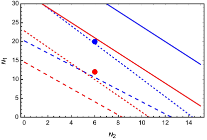
Figure 2: Conformal window as a function of the number of Weyl spinors in the fundamental ($N_{1}$) and antisymmetric ($N_{2}$) for $Sp(4)_{\rm HC}$ (red) and $SU(4)_{\rm CHC}$ (blue). The solid line indicates where asymptotic freedom is lost, while the dashed and dotted lines indicate the expected lower edge using the PS or SD methods, respectively.

A key ingredient for any composite Higgs model with top partial compositeness is the presence of a near-conformal “walking” dynamics above the condensation scale $\Lambda_{\rm HC}$. This may ensure that the hyper-baryons that couple to the top develop a large anomalous dimensions, which in turn can enhance the top PC couplings at low energy. For this mechanism to have any hope to work, the theory in the walking phase should lie as close as possible to the lower edge of the conformal window, thus being in a strongly coupled regime. Unfortunately, estimating the location of the conformal edge in terms of the fermion multiplicities is subject to many uncertainties, due to the strong coupling. In the following, we will adopt two methods developed in the literature: the Pica-Sannino (PS) all order beta function Pica:2010mt , and the Schwinger-Dyson (SD) equation approach Sannino:2009za . The former is based on a conjectured all-order beta function that depends on the mass anomalous dimensions of the fermions charged under the running gauge coupling. In the conformal window, the beta function should vanish, while the mass anomalous dimensions are expected to be of order unity. Thus, this provides enough constraints to fix the number of fermions, leading to

$$11C_{2}(G)-\sum_{r}T(r)n_{r}\left(3+\frac{7}{11}\frac{C_{2}(G)}{C_{2}(r)}\right)=0\,,$$ (36)

where $C_{2}$ is the Casimir and $T$ the dynkin index of the representation ($G$ indicates the adjoint), while $n_{r}$ is the number of Weyl fermions in the representation $r$. The latter method, based on the ladder approximation in the gap equation, makes use of the fact that the anomalous mass dimension at one loop equals 1 at the critical value of the gauge coupling where chiral symmetry is broken. This can be compared to the zero of the beta function, which first appears at two loops, leading to

$$\alpha^{\ast}=-\frac{4\pi\beta_{0}}{\beta_{1}}=\frac{2\pi}{3C_{2}(r)}\,.$$ (37)

As we have two different representations, we will consider the one whose anomalous dimension reaches unity first, i.e. the antisymmetric.

We first apply these methods to a $Sp(4)_{\rm HC}$ theory Sannino:2009aw with $N_{1}$ Weyl spinors in the fundamental and $N_{2}$ Weyl spinors in the antisymmetric. The result is shown in Fig. 2 by the red lines, where the dashed (dotted) correspond to the PS (SD) method. In solid we show the line above which asymptotic freedom is lost. This case is relevant for the TPS model when the CHC breaking occurs at high scale, i.e. before the onset of the walking phase. The model we presented in this section contains $N_{2}=6$ degrees of freedom in the antisymmetric representation, coming from the $\Xi$ multiplet. For $N_{2}=6$, the PC method gives the lower edge starting at $N_{1}=5$, while for SD it starts at $N_{1}=10$ (while asymptotic freedom is lost for $N_{1}=21$). To compare with a realistic scenario, we recall that one SM generation ($\Omega$ + $\Upsilon$) plus a $\Xi$ contains $N_{1}=12$, which is inside the conformal window (C.f., red dot in Fig. 2), and very close to the boundary according to the SD method. Thus, if SD is correct, the model has good chances of being close to the edge and develop large anomalous dimensions. We anticipate that extending to 3 generations would minimally require to add a flavor index to $\Omega$ and $\Upsilon$, raising the number of fundamental hyper-fermions to $N_{1}=20$, which is well too close to the edge of asymptotic freedom loss, where the theory becomes weakly coupled. This simple analysis shows that the hyper-fermions associated to the light generations should not be light, feature that we will exploit in the next sections.

It is also interesting to consider the case where the CHC symmetry is only broken at low energies, after the model enters the walking phase. As the hyper-fermions contained in $\Omega$ and $\Upsilon$ inherit the chiral structure of the SM fermions, they cannot acquire a mass before CHC is broken. Thus, the minimal model with three generations will have $N_{1}=20$. The case of $SU(4)_{\rm CHC}$ Ryttov:2009yw is shown in Fig. 2 in blue, with the same conventions as above: the conformal window edge is expected at $N_{1}=11$ with the PS method, and $N_{1}=20$ with SD (while the asymptotic freedom loss occurs at $N_{1}=32$) The minimal model, represented by the blue dot, is again very close to the SD lower edge of the conformal window. The case with low scale CHC breaking is therefore also interesting. However, it can only occur if a mechanism that generates a large hierarchy between the VEVs of various scalars is understood. In the following we will focus on the case of high scale CHC breaking, leaving the low scale case for further investigation.

The theory we consider in the following, therefore, features the $Sp(4)_{\rm HC}$ dynamics in a walking regime between $\Lambda_{\rm HC}$ and $\Lambda_{F}$. As a further consistency check, as many fermions are present in this wide energy range, we checked that the running of the SM gauge couplings, $g_{3}$ for QCD, $g_{2}$ for $SU(2)_{L}$ and $g_{Y}$ for hypercharge do not develop a Landau pole before the $\Lambda_{\rm PU}$ scale. We thus used PyR@TE Lyonnet:2013dna ; Lyonnet:2016xiz to compute the running where only one generation of hyper-fermions is included (i.e., $N_{1}=12$). The two-loop running is shown in Fig. 3, proving that the gauge couplings remain under control. These results are mainly qualitative, as the contribution of the HC gauge coupling, which is strong, has not been included. There might be concern that $g_{3}\sim 1$ is too perturbative around $\sim 10^{16}~{}{\mbox{GeV}}$ where it unifies with $SU(4)_{CHC}$, so that the resulting $Sp(4)_{HC}$ coupling might spend unacceptably long RG time in the perturbative regime. However, the ignored HC correction might alter the evolution of $g_{3}$ so that $SU(4)_{CHC}$ and $SU(3)_{C}$ unify at some semi-perturbative value, which we will assume. Also, above the PU scale, the two $SU(2)$ gauge couplings keep growing as their beta function has lost asymptotic freedom: including 3 generation of $\Omega$ and $\Upsilon$, each has $3\times 8$ Weyl spinors. However, this may be a minor issue, because the Planck scale is close to $\Lambda_{\rm PU}$ by construction, where quantum gravity effects should start to be relevant and may tame the growth of the gauge couplings Eichhorn:2018yfc .

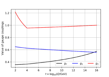
Figure 3: Perturbative evolution of SM gauge couplings. Two-loop effects from SM gauge interactions are taken into account, while HC corrections are not included.

III Techni-Pati-Salam for the Third Family

In this section, we will first construct a model that provides masses for one generation of SM fermions, namely the third one, as this exercise allows to better illustrate the main properties of the model. Extension to 3 generations will be presented in the next section. The minimal field content is listed in Table 2. We add all the scalars discussed in the previous section in order to keep open both paths of symmetry breaking and also, as we will see, because they all play a crucial role in generating SM fermion masses.

Field	Spin	$SU(8)_{\rm PS}$	$SU(2)_{L}$	$SU(2)_{R}$	$Q_{G}$
$\Phi$	$0$	8	1	2	$q$
$\Theta$	$0$	28	1	1	$2q$
$\Delta$	$0$	56	1	2	$q$
$\Psi$	$0$	63	1	1	$0$
$N$	$1/2$	1	1	1	$0$
$\Omega$	$1/2$	8	2	1	$q$
$\Upsilon$	$1/2$	$\overline{\textbf{8}}$	1	2	$-q$
$\Xi$	$1/2$	70	1	1	$0$

Table 2: Scalar and (left-handed Weyl) fermion field content. The last column indicates the global $U(1)_{G}$ charges, with $q\neq 0$ being an arbitrary normalization factor.

III.1 Lagrangian and gauge-mediated PC4F Operators

The complete Lagrangian of the model, including only renormalizable operators, can be decomposed as

$$\mathcal{L}_{\rm TPS^{3}}=\mathcal{L}_{G}+\mathcal{L}_{F}+\mathcal{L}_{S}+\mathcal{L}_{Y}+\mathcal{L}_{V}\,,$$ (38)

where $\mathcal{L}_{G}$, $\mathcal{L}_{F}$ and $\mathcal{L}_{S}$ denote the kinetic terms for gauge, fermion and scalar fields respectively (including gauge interactions), $\mathcal{L}_{Y}$ contains the fermion bare mass terms and Yukawa interactions, while $\mathcal{L}_{V}=-V(\Phi,\Theta,\Delta,\Psi)$ is the scalar potential term. For our purposes, the most relevant part is $\mathcal{L}_{Y}$, which is given explicitly by:

$$\mathcal{L}_{Y} =-\frac{1}{2}\mu_{N}NN-\frac{1}{2}\mu_{\Xi}\Xi\Xi-\frac{1}{2}\lambda_{\Psi}\Xi\Psi\Xi-\left(\lambda_{\Phi}\Upsilon\Phi N\right.$$

$$\left.+\lambda_{\Theta L}\Omega\Theta^{*}\Omega+\lambda_{\Theta R}\Upsilon\Theta\Upsilon+\lambda_{\Delta}\Upsilon\Delta^{*}\Xi+\text{h.c.}\right)\,,$$ (39)

where the first three terms are self-hermitian. In principle, the Yukawas $\lambda_{i}$ (except $\lambda_{\Psi}$) are complex parameters, however one can use arbitrary phase redefinitions of the fermion and scalar fields to make all of them real, without loss of generality. At this stage, therefore, physical phases can only be contained in the scalar potential $\mathcal{L}_{V}$. The interaction terms in $\mathcal{L}_{Y}$ (including the kinetic terms) also leave a global $U(1)_{G}$ unbroken, with charges defined in Table 2. Explicit $U(1)_{G}$-breaking terms may appear in the scalar potential. We assume minimizing the scalar potential leads to the desired VEV configuration that break the PS, EHC and CHC groups (see discussion in Sec. II.2).

The gauge couplings relevant for generating PC4F operators involve only 2 of the massive gauge bosons, deriving from the PS and EHC breaking: $E_{\mu}=({\bf 4},{\bf 3})_{1/6}$ and $C_{\mu}=({\bf 4},{\bf 1})_{1/2}$ . Their couplings read 

$$\mathcal{L}_{F}\supset\frac{g_{\rm PS}}{\sqrt{2}}\ C_{\mu}J_{C}^{\mu}+\frac{g_{\rm EHC}}{\sqrt{2}}\ E_{\mu}J_{E}^{\mu}+\text{h.c.}\,,$$ (40)

where $g_{\rm PS}$ and $g_{\rm EHC}$ are the gauge couplings of $SU(8)_{\rm PS}$ and $SU(7)_{\rm EHC}$ respectively, with $g_{\rm EHC}\approx g_{\rm PS}$ if the breaking of the two symmetries is happening at closeby scales. The two currents read:

$$J_{E}^{\mu}=\bar{q_{L}}\bar{\sigma}^{\mu}L^{3}-\bar{D}_{u}^{3}\bar{\sigma}^{\mu}t_{R}^{c}-\bar{U}_{d}^{3}\bar{\sigma}^{\mu}b_{R}^{c}+\frac{1}{2}\left(\bar{\chi}\bar{\sigma}^{\mu}U_{t}-\bar{D}_{b}\bar{\sigma}^{\mu}\tilde{\chi}\right)-\left(\bar{\eta}\bar{\sigma}^{\mu}\chi-\bar{\tilde{\chi}}\bar{\sigma}^{\mu}\tilde{\eta}\right)\\ -\left(\bar{\eta}\bar{\sigma}^{\mu}\omega-\bar{\tilde{\omega}}\bar{\sigma}^{\mu}\tilde{\eta}\right)+\frac{1}{2}\left(\bar{\rho}\bar{\sigma}^{\mu}\eta-\bar{\tilde{\eta}}\bar{\sigma}^{\mu}\tilde{\rho}\right)+\frac{1}{2}\left(\bar{\omega}\bar{\sigma}^{\mu}U_{t}-\bar{D}_{b}\bar{\sigma}^{\mu}\tilde{\omega}\right)\,,$$ (41)

$$J_{C}^{\mu}=\bar{L}^{3}\bar{\sigma}^{\mu}l_{L}-\bar{\nu}_{\tau R}^{c}\bar{\sigma}^{\mu}D_{u}^{3}-\bar{\tau}_{R}^{c}\bar{\sigma}^{\mu}U_{d}^{3}-\frac{1}{2}\left(\bar{\tilde{\eta}}\bar{\sigma}^{\mu}\chi+\bar{\tilde{\chi}}\bar{\sigma}^{\mu}\eta\right)-\frac{1}{2}\left(\bar{\tilde{\eta}}\bar{\sigma}^{\mu}\omega+\bar{\tilde{\omega}}\bar{\sigma}^{\mu}\eta\right)-\frac{1}{6}\left(\bar{\tilde{\rho}}\bar{\sigma}U_{t}+\bar{D}_{b}\bar{\sigma}\rho\right)\,.$$ (42)

By integrating out the two vector mediators, we obtain the following four fermion operators, linear in the SM fields:

$$\mathcal{L}_{\rm PC4F}\supset-\frac{g_{\rm EHC}^{2}}{2M_{E}^{2}}\ \left(\bar{L}^{3}\bar{\sigma}^{\mu}q_{L}-\bar{t}_{R}^{c}\bar{\sigma}^{\mu}D_{u}^{3}-\bar{b}_{R}^{c}\bar{\sigma}^{\mu}U_{d}^{3}\right)\left(\frac{1}{2}\bar{\chi}\bar{\sigma}_{\mu}U_{t}-\frac{1}{2}\bar{D}_{b}\bar{\sigma}_{\mu}\tilde{\chi}-\bar{\eta}\bar{\sigma}_{\mu}\chi+\bar{\tilde{\chi}}\bar{\sigma}_{\mu}\tilde{\eta}\right)\\ -\frac{g_{\rm PS}^{2}}{2M_{C}^{2}}\ \left(\bar{L}^{3}\bar{\sigma}^{\mu}l_{L}-\bar{\nu}_{\tau R}^{c}\bar{\sigma}^{\mu}D_{u}^{3}-\bar{\tau}_{R}^{c}\bar{\sigma}^{\mu}U_{d}^{3}\right)\left(-\frac{1}{2}\bar{\chi}\bar{\sigma}_{\mu}\tilde{\eta}-\frac{1}{2}\bar{\eta}\bar{\sigma}_{\mu}\tilde{\chi}\right)\,.$$ (43)

The interesting property of Eq. (43) is that all quark operators are mediated by $E_{\mu}=(\textbf{4},\textbf{3})_{1/6}$, which becomes massive from the EHC breaking, while all lepton operators are mediated by $C_{\mu}=(\textbf{4},\textbf{1})_{1/2}$, which becomes massive from the PS breaking. The mass hierarchy between leptons and quarks could, therefore, be explained by a hierarchy in the masses of the mediators if $M_{C}>M_{E}$ (see Sec. II.2). Furthermore, lepton operators always involve the QCD-colored hyper-fermions $\eta$–$\tilde{\eta}$, while the quark ones also involve the QCD-singlets $U_{t}$ and $D_{b}$.

It is remarkable that our PUPC approach allows to generate appropriate PC4F operators for all SM quarks from gauge interactions, however there is no distinction between fermions in the same weak isospin multiplet. In other words, the gauge interactions themselves cannot distinguish between top-bottom, nor between tau-neutrino. Such mass splittings, which need violation of $SU(2)_{R}$, naturally receive contributions in our model: from scalar mediated PC4F operators, from the masses of the involved hyper-fermions, and, in the case of the neutrino, from mixing with the singlet $N$ via $\lambda_{\Phi}$. These effects are discussed in the following sub-sections.

1 SM field

0 SM field

$\Big{(}$ $\varphi_{i}$

$({\bf 4},{\bf 1})_{-\frac{1}{2}}$

$({\bf 4},{\bf 3})_{\frac{1}{6}}$

$({\bf 4},{\bf 3})_{-\frac{5}{6}}$

$({\bf 5},{\bf 1})_{0}$

$({\bf 5},{\bf 1})_{-1}$

$({\bf 5},{\bf 3})_{\frac{2}{3}}$

$({\bf 5},{\bf 3})_{-\frac{1}{3}}$

$({\bf 4},{\bf 1})_{\frac{1}{2}}$

$({\bf 4},{\bf 3})_{\frac{1}{6}}$

$({\bf 4},{\bf 3})_{-\frac{5}{6}}$

$({\bf 5},{\bf 1})_{0}$

$({\bf 5},{\bf 1})_{-1}$

$({\bf 5},{\bf 3})_{\frac{2}{3}}$

$({\bf 5},{\bf 3})_{-\frac{1}{3}}$

$\Omega\Theta^{\ast}\Omega$

$(L^{3}l_{L})$

$(L^{3}q_{L})$

-

-

-

-

-

-

-

-

$(L^{3}L^{3})$

-

-

-

$\Upsilon\Theta\Upsilon$

$(U_{d}^{3}\nu_{R}^{c})$

$(U_{d}^{3}t_{R}^{c})$

-

-

-

-

-

-

-

-

$(U_{d}^{3}D_{u}^{3})$

-

-

-

$(D_{u}^{3}\tau_{R}^{c})$

$(D_{u}^{3}b_{R}^{c})$

-

-

-

-

-

-

-

-

-

-

-

$\Xi\Psi\Xi$

-

-

-

-

-

-

-

$(\chi D_{b})$

-

$(U_{t}D_{b})$

-

-

-

$(U_{t}\tilde{\chi})$

$(\chi\eta)$

$(\eta\tilde{\chi})$

$(\eta\tilde{\eta})$

$(\tilde{\chi}\tilde{\eta})$

$(\chi\tilde{\eta})$

$\Upsilon\Delta^{\ast}\Xi$

$(U_{t}\nu_{R}^{c})$

$(D_{b}t_{R}^{c})$

$(D_{b}b_{R}^{c})$

-

$(\chi U_{d}^{3})$

$(\chi D_{u}^{3})$

$(U_{t}U_{d}^{3})$

$(U_{t}D_{u}^{3})$

$(\tilde{\eta}U_{d}^{3})$

$(\tilde{\eta}D_{u}^{3})$

$(U_{t}\tau_{R}^{c})$

$(\tilde{\eta}t_{R}^{c})$

$(\eta b_{R}^{c})$

$(\eta t_{R}^{c})$

$(\chi b_{R}^{c})$

$(\chi t_{R}^{c})$

$(\tilde{\chi}b_{R}^{c})$

$(\tilde{\chi}t_{R}^{c})$

$(\tilde{\chi}D_{u}^{3})$

$(\tilde{\chi}U_{d}^{3})$

$(\tilde{\eta}b_{R}^{c})$

$(\eta\nu_{R}^{c})$

$(\eta\tau_{R}^{c})$

$(\chi\tau_{R}^{c})$

$(\chi\nu_{R}^{c})$

Table 3: Scalar mediators $\varphi_{i}$ (quantum numbers listed in the top row), with the fermion bilinears they couple with. The rows correspond to different Yukawa interactions from $\mathcal{L}_{Y}$. The fermion bilinears in red couple to the conjugate scalar, $\varphi_{i}^{\ast}$.

III.2 Scalar mediated PC4F operators

The Yukawa couplings in $\mathcal{L}_{Y}$, Eq. (39), allow for many scalar components to mediate PC4F operators. All the relevant combinations are listed in Table 3, where we have identified 7 distinct mediators, whose quantum numbers are listed in the top row. The rows correspond to different Yukawa couplings, while the left block “1 SM field” contains fermion bilinears containing one SM field and the right one “0 SM field” bilinears involves only hyper-fermions. The PC4F operators can thus be constructed by coupling one fermion bilinear from the left block with one from the right block, if they have matching quantum numbers. If they belong to different Yukawa couplings, the resulting operator can only be generated if the components in the two scalar multiplets mix. As an example, the mediators $\varphi_{4}=({\bf 5},{\bf 1})_{0}$ and $\varphi_{5}=({\bf 5},{\bf 1})_{-1}$, components of $\Delta$, will generate the following PC4F operators for right-handed top and bottom:

$$\mathcal{L}_{\rm PC4F}\supset-\frac{\lambda_{\Delta}^{2}}{M_{\varphi_{4}}^{2}}c_{4}\ (\overline{U}_{t}\overline{U}_{d}^{3})(\chi b_{R}^{c})-\frac{\lambda_{\Delta}^{2}}{M_{\varphi_{5}}^{2}}c_{5}\ (\overline{U}_{t}\overline{D}_{u}^{3})(\chi t_{R}^{c})\,,$$ (44)

where $c_{4,5}$ are group theory factors. This example illustrates how a mass splitting between top and bottom could arise if the above couplings are dominant, and there exist a significant mass difference between the two scalar mediators. Scalar-mediated PC4F operators are subject to a larger degree of arbitrariness compared to vector-mediated PC4F operators, because their strengths are determined by the non-universal Yukawa couplings, and masses and mixing of scalar components controlled by details of the scalar potential. Nevertheless, they are also generated automatically from the renormalizable Lagrangian, rather than being put in by hand.

The main ingredients that determine the relevance of scalar mediated PC4F operators are the following:

• the masses and mixing pattern of the scalars.

• the size of the Yukawa couplings. As we will see in the next section, the masses of the hyper-fermions also depend on some of these Yukawas. To keep some hyper-fermions light, therefore, a number of Yukawas need to be small, thus also being ineffective in generating sizable PC4F operators.

In the next 3 subsections, we will discuss the impact of the Yukawa couplings on the hyper-fermion masses, and list the concrete ways the model allows to generate the top-bottom mass hierarchy and small neutrino masses.

III.3 Hyper-fermion masses

Hyper-fermion masses play an important role in determining the properties of the model. Firstly, the low-energy global symmetry pattern is determined by the number of hyper-fermions that are lighter than the hypercolor condensation scale $\Lambda_{\rm HC}\sim 10~{}{\mbox{TeV}}$. Secondly, whether the HC dynamics enters a strongly-coupled near-conformal regime above $\Lambda_{\rm HC}$ depends on the additional hyper-fermions that have a mass between $\Lambda_{\rm HC}$ and $\Lambda_{\rm EHC}$, as discussed in Sec. II.3. Thirdly, the mass of the hyper-fermions participating in the PC4F operators determines the masses of the corresponding SM fermions: assuming that the dominant contribution is coming from local insertions of the PC4F operators, the SM fermion mass is proportional to the corresponding Fourier-transformed two-point hyperbaryon correlator at zero momentum Golterman:2015zwa . When one of the participating hyper-fermions is heavier than $\Lambda_{\rm HC}$, the correlator is expected to be suppressed by some power of the hyper-fermion mass, as it can be analyzed via the Shifman-Vainshtein-Zakharov (SVZ) expansion Shifman:1978bx ; Shifman:1978by .

Let’s start the discussion with the hyper-fermions $\chi$–$\tilde{\chi}$ and $\eta$–$\tilde{\eta}$: they enter in all PC4F operators for quarks and leptons, thus they cannot be too heavy. In particular, as all quark operators, both from gauge and scalar mediation, contain $\chi$ or $\tilde{\chi}$, while all fermion operators contain $\eta$ or $\tilde{\eta}$, in order to obtain a large enough top and tau masses it would be optimal to have $M_{\chi}\leq\Lambda_{\rm HC}$ and $M_{\eta}\leq\mathcal{O}(10)\times\Lambda_{\rm HC}$. Furthermore, a hierarchy $M_{\chi}<M_{\eta}$ could explain why leptons are lighter than quarks. These hyper-fermion masses receive contributions only from the $\Xi$ mass term and from the Yukawa $\lambda_{\Psi}$ via the $\Psi$ VEV, resulting in the following terms

$$\mathcal{L}_{Y} \supset-\mu_{0}U_{t}D_{b}-(\mu_{0}-5\mu_{1})(\tilde{\chi}\chi+\tilde{\omega}\omega)$$

$$-(\mu_{0}+2\mu_{1})\tilde{\eta}\eta-\mu_{0}\tilde{\rho}{\rho}+\text{h.c.}$$ (45)

where

$$\mu_{0}\propto\mu_{\Xi}\,,\qquad\mu_{1}\propto\lambda_{\Psi}v^{\Psi}_{\rm EHC}\,.$$ (46)

Note that, as expected, $\mu_{0}$ is a universal term for all components of $\Xi$, while $\mu_{1}$ only contributes to a sub-set of them. Thus, we can identify

$$M_{\chi}=|\mu_{0}-5\mu_{1}|\,,\qquad M_{\eta}=|\mu_{0}+2\mu_{1}|\,,$$ (47)

while the masses of the other components receive additional contributions via mixing, as we will discuss below. The desired hierarchy $M_{\chi}<M_{\eta}$ is thus achieved for $0<\mu_{1}<\frac{2}{3}\mu_{0}$, where we have assumed $\mu_{0}>0$ without loss of generality. The value of the parameter $\mu_{0}$, which contributes to the mass of the singlet $\rho$–$\tilde{\rho}$ and of the hyper-fermions $U_{t}$–$D_{b}$, is related to the two masses by the inequality

$$\mu_{0}\leq\frac{2}{7}M_{\chi}+\frac{5}{7}M_{\eta}\,,$$ (48)

implying that is tends to be smaller than the two masses. An important lesson we can take from this analysis is that, barring fine cancellations, $\mu_{0},\mu_{1}\ll\Lambda_{EHC}$, which implies that the Yukawa $\lambda_{\Psi}$ needs to be very small. This is technically natural, however it has an important consequence on the scalar mediated PC4F operators: the ones stemming from $\Xi\Psi\Xi$ (see Table 3) are highly suppressed.

We can now discuss the masses of the QCD-singlet hyper-fermions, $L^{3}$, $D_{u}^{3}$, $U_{d}^{3}$, $U_{t}$ and $D_{b}$, which are relevant for generating the composite Higgs at low energy. The pNGB Higgs, in fact, is a bound state of $L^{3}$ and one of the weak iso-singlets: this implies that one needs $L^{3}$ and one set of the iso-singlets to be much lighter that $\Lambda_{\rm HC}$. While the $\Xi$ components $U_{t}$–$D_{b}$ receive a mass from Eq. (45), the other hyper-fermions receive a mass via the $\Theta$-VEV as follows:

$$\mathcal{L}_{Y}\supset-\mu_{L}L^{3}L^{3}-\mu_{R}U_{d}^{3}D_{u}^{3}\,,$$ (49)

where

$$\mu_{L}=\lambda_{\Theta L}v^{\Theta}_{\rm CHC}\,,\qquad\mu_{R}=\lambda_{\Theta R}v^{\Theta}_{\rm CHC}\,.$$ (50)

For the iso-doublet, this is the only contribution to the mass, so that $M_{L}=\mu_{L}$. To keep this mass small, there are three possibilities: a) $\lambda_{\Theta L}\ll 1$ and $v^{\Theta}_{\rm CHC}\gg\Lambda_{\rm HC}$, thus the scalar-mediated PC4F operators cannot receive contributions from $\Omega\Theta^{\ast}\Omega$; b) $\lambda_{\Theta L}\lesssim 1$ and $v^{\Theta}_{\rm CHC}\geq\Lambda_{\rm HC}$; c) $v^{\Theta}_{\rm CHC}=0$. In the last two cases the Yukawa could give sizable contributions to scalar-mediated PC4F operators. In the case of the iso-singlets, mixing terms are also generated in the presence of VEVs for $\Delta$, in the form

$$\mathcal{L}_{Y} \supset-\mu_{\Delta 1}\left(D_{u}^{3}D_{b}-\nu_{\tau R}^{c}\rho\right)$$

$$-\mu_{\Delta 2}\left(U_{d}^{3}U_{t}+\sqrt{2}b_{R}^{c}\omega\right)+\text{h.c.}$$ (51)

where

$$\mu_{\Delta 1}=\lambda_{\Delta}v^{\Delta}_{\rm EHC}\,,\qquad\mu_{\Delta 2}=\lambda_{\Delta}v^{\Delta}_{\rm CHC}\,.$$ (52)

Note that these two terms also induce a mixing of $\rho$ with the neutrinos, and of $\omega$ with the right-handed bottom. We will come back to their effect in the next two subsections. In the hyper-fermion sector, this leads to the following mass matrix:

$$\mathcal{L}_{Y} \supset-\begin{pmatrix}U_{d}^{3}&D_{b}\end{pmatrix}\begin{pmatrix}\mu_{R}&\mu_{\Delta 2}\\ \mu_{\Delta 1}&\mu_{0}\end{pmatrix}\begin{pmatrix}D_{u}^{3}\\ U_{t}\end{pmatrix}+\text{h.c.}\,,$$ (53)

which has eigenvalues

$$M_{R1,2}^{2} =\frac{1}{2}\left(\tilde{\mu}^{2}\mp\sqrt{\tilde{\mu}^{4}-4(\mu_{0}\mu_{R}-\mu_{\Delta 1}\mu_{\Delta 2})^{2}}\right)\,,$$

$$\mbox{with}\;\;\tilde{\mu}^{2}=\mu_{0}^{2}+\mu_{R}^{2}+\mu_{\Delta 1}^{2}+\mu_{\Delta 2}^{2}\,.$$ (54)

We see that one can achieve at least one small mass eigenvalue if either all $\mu$’s are small, or

$$2(\mu_{0}\mu_{R}-\mu_{\Delta 1}\mu_{\Delta 2})\ll\tilde{\mu}^{2}\,.$$ (55)

Seen the constraints on $\mu_{0}$ coming from the $\chi$ and $\eta$ masses, the latter condition may be achieved for

a) $$\mu_{R}\ll\mu_{0}\,,\;\;\mu_{\Delta 1}\mu_{\Delta 2}\ll\mu_{0}^{2}\,,$$

$$\Rightarrow M_{R1}\approx\left|\mu_{R}-\frac{\mu_{\Delta 1}\mu_{\Delta 2}}{\mu_{0}}\right|\,,\;\;M_{R2}\approx\mu_{0}\,;$$ (56)

or

b) $$\mu_{0}\ll\mu_{R}\,,\;\;\mu_{\Delta 1}\mu_{\Delta 2}\ll\mu_{R}^{2}\,,$$

$$\Rightarrow M_{R1}\approx\left|\mu_{0}-\frac{\mu_{\Delta 1}\mu_{\Delta 2}}{\mu_{R}}\right|\,,\;\;M_{R2}\approx\mu_{R}\,.$$ (57)

In the latter case, if $\mu_{R}\geq\Lambda_{\rm HC}$, one could have that only one mass eigenstate is below the condensation scale, while in the former typically both are light. One can see, therefore, that the masses have a crucial impact on the low energy dynamics of the theory by influencing the global coset that determines the properties of the composite Higgs:

$$M_{R2}\geq\Lambda_{\rm HC}\Leftrightarrow\frac{SU(4)}{Sp(4)}\;\;\mbox{\cite[cite]{\@@bibref{Authors Phrase1YearPhrase2}{Galloway:2010bp,Cacciapaglia:2014uja}{\@@citephrase{(}}{\@@citephrase{)}}}}\,,$$

$$M_{R2}\ll\Lambda_{\rm HC}\Leftrightarrow\frac{SU(6)}{Sp(6)}\;\;\mbox{\cite[cite]{\@@bibref{Authors Phrase1YearPhrase2}{Cai:2018tet}{\@@citephrase{(}}{\@@citephrase{)}}}}\,.$$

We also remark that, keeping $\mu_{\Delta 1}\mu_{\Delta 2}$ small would imply either $\lambda_{\Delta}\ll 1$, or a large hierarchy between the VEVs, $v^{\Delta}_{\rm CHC}\ll v^{\Delta}_{\rm EHC}$, with the extreme case $v^{\Delta}_{\rm CHC}=0$. These various possibilities have an important impact on the scalar PC4F sector, by determining which terms can be sizable and which ones are always suppressed. The implications for the masses of leptons and quarks will be discussed in the following two subsections.

We recall that the patterns of hyper-fermion masses depend crucially on the pattern of VEVs that break the TPS group down to the low energy theory. In this discussion we work under the assumption that the desired vacuum misalignment and EWSB can be achieved, leaving a detailed study of the vacuum misalignment mechanism to future work Giacomo:2019ehd .

To conclude, we would like to recap the main findings in two special cases of VEV patterns, following the discussion in Sec. II.2.

• $\langle\Delta\rangle=0$. In this case, the EHC breaking is due to $v^{\Psi}_{\rm EHC}$, while $v^{\Theta}_{\rm CHC}$ breaks $SU(4)_{\rm CHC}$ down to $Sp(4)_{\rm HC}$. The mixing terms between iso-singlet hyper-fermions vanish, so that we have a simple mass pattern:

  $$M_{L}=\mu_{L}\,,\;\;M_{R1}=\mbox{min}\{\mu_{R},\mu_{0}\}\,,$$

  $$M_{R2}=\mbox{max}\{\mu_{R},\mu_{0}\}\,.$$ (58)

  Furthermore, the HC-singlets $\omega$ and $\rho$ do not mix and have masses

  $$M_{\omega}=M_{\chi}\,,\;\;M_{\rho}=\mu_{0}\,.$$ (59)

  The only large Yukawa is therefore $\lambda_{\Delta}$, which is responsible for generating scalar PC4F operators (one could also have sizable $\lambda_{\Theta L/R}$ if $v^{\Theta}_{\rm CHC}\approx\Lambda_{\rm HC}$). Note that keeping $M_{\chi}$ below $\Lambda_{\rm HC}$ requires small $\mu_{1}$, where the hierarchy $M_{\chi}<M_{\eta}$ can be kept for $0<\mu_{1}<2/3\ \mu_{0}$.

• $\langle\Theta\rangle=\langle\Psi\rangle=0$. In this case, both EHC and CHC breaking is due to VEVs of the field $\Delta$. As $\mu_{1}=\mu_{L}=\mu_{R}=0$, we have

  $$M_{\chi}=M_{\eta}=\mu_{0}\,,\;\;M_{L}=0\,,$$ (60)

  while the iso-singlet masses are given by Eq.(57) with $\mu_{R}=0$. At least one light eigenstate can be achieved by keeping the mixing terms small, thus requiring $\lambda_{\Delta}\ll 1$ (and the corresponding Yukawa ineffective in generating scalar PC4F operators).

III.4 Top-Bottom Mass Splitting

The SM features a large hierarchy between top and bottom masses, with $m_{t}/m_{b}\sim 60$ at the weak scale. In the TPS model, the top-bottom mass splitting must be traced back to spontaneous $SU(2)_{R}$-breaking. We identified three effects that may explain this feature, which we analyse in detail below.

Firstly, we noted that gauge mediators as well as scalar mediators from the $\Upsilon\Theta\Upsilon$ Yukawa cannot be used as they contain both $b_{R}^{c}$ and $t_{R}^{c}$. However, scalar-mediated PC4F operators constructed from $\Upsilon\Delta\Xi$ involve mediators that differ in type and properties for $t_{R}^{c}$ and $b_{R}^{c}$, as it can be seen in Table 3. Thus, a split between top and bottom can simply arise from a difference in mass between the two mediators. One example shown in Eq. (44) involves $\varphi_{4}=({\bf 5},{\bf 1})_{0}$ and $\varphi_{5}=({\bf 5},{\bf 1})_{-1}$. Another example involves $\varphi_{2}=({\bf 4},{\bf 3})_{1/6}$ and $\varphi_{3}=({\bf 4},{\bf 3})_{-5/6}$. In both cases, the scalar mass difference breaks $SU(2)_{R}$, and a sizable coefficient can arise from a large $\lambda_{\Delta}$, allowed for vanishing $\Delta$ VEV.  Another source of mass split lies in the fact that the quantum number $(\textbf{5},\textbf{1})_{0}$ has more ways of pairing compared to $(\textbf{5},\textbf{1})_{-1}$ since it also appears in Yukawa terms other than $\Upsilon\Delta\Xi$. Note this is not incompatible with the fact that the Yukawa Lagrangian explicitly preserves $SU(2)_{R}$ which is a gauge symmetry. The reason is that the required mixing between scalar components with quantum number $(\textbf{5},\textbf{1})_{0}$ can only occur if there exists spontaneous $SU(2)_{R}$-breaking from the scalar potential. Let us also note that this mechanism does not lead to a prediction of the top-bottom mass splitting, nor a prediction of which quark is heavier, because these properties sensitively depend on details of the scalar potential.

Secondly, a differentiation of top and bottom may come from the mixing in the iso-singlet hyper-fermion sector, given by Eq. (53). This opens the possibility that the top has a larger coupling to the lighter mass eigenstate, while the bottom dominantly couples to the heavier one, thus having its mass suppressed. To be more specific, we can analyse the case of dominant gauge mediation: from Eq. (41) we see that $t_{R}^{c}$ couples to $D_{u}^{3}$, while $b_{R}^{c}$ to $U_{d}^{3}$. As the mixing angles for the pairs $D_{u}^{3}$–$U_{t}$ and $U_{d}^{3}$–$D_{b}$ are different if $\mu_{\Delta 1}\neq\mu_{\Delta 2}$, one can easily generate hierarchical mixing angles. For instance, for $\mu_{R}=0$ (achieved if $\langle\Theta\rangle=0$) the mixing relevant for the top is proportional to $\mu_{\Delta 2}$, while the one for the bottom to $\mu_{\Delta 1}$. As

$$\frac{\mu_{\Delta 1}}{\mu_{\Delta 2}}\propto\frac{v^{\Delta}_{\rm EHC}}{v^{\Delta}_{\rm CHC}}>1\,,$$ (61)

a larger mixing angle for the bottom is assured. Another interesting possibility is that both iso-singlet hyper-fermions remain light, in which case the theory features two Higgs doublets in the IR, and the mass hierarchy may be due to the distribution of the EW VEV on the two doublets Rosenlyst:2020znn , as in traditional 2HDM Branco:2011iw .

Thirdly, the most interesting mechanism sprouts from the mixing between $b_{R}^{c}$ and $\omega$, see Eq. (51). As no such term exists for the top quark, this mixing leads to a suppression of the bottom mass. The complete mass term reads

$$\mathcal{L}_{Y}\supset-\omega\left((\mu_{0}-5\mu_{1})\tilde{\omega}+\sqrt{2}\mu_{\Delta 2}b_{R}^{c}\right)+\text{h.c.}$$ (62)

Thus we can define mass eigenstates as

$$B_{L}=\omega\,,\;\; B_{R}^{c}=\cos\alpha_{b}\ \tilde{\omega}+\sin\alpha_{b}\ b_{R}^{c}\,,$$

$$\tilde{b}_{R}^{c}=\cos\alpha_{b}\ b_{R}^{c}-\sin\alpha_{b}\ \tilde{\omega}\,,$$ (63)

where

$$\tan\alpha_{b} =\text{sign}(\mu_{0}-5\mu_{1})\ \frac{\sqrt{2}\mu_{\Delta 2}}{M_{\chi}}\,,$$ (64)

$$M_{B} =\sqrt{M_{\chi}^{2}+2\mu_{\Delta 2}^{2}}\geq M_{\chi}\,,$$ (65)

while $\tilde{b}_{R}^{c}$ can be identified with the (massless) right-handed bottom. In the case of gauge mediation, the current in Eq. (41) can be re-written as

$$J_{E}^{\mu}\supset\left(-\cos(\alpha_{b})\bar{U}_{d}^{3}-\frac{1}{2}\sin(\alpha_{b})\bar{D}_{b}\right)\bar{\sigma}^{\mu}\tilde{b}_{R}^{c}+\dots$$ (66)

Combined with the mixing between $U_{d}^{3}$–$D_{b}$, this could lead to a suppressed coupling of the right-handed bottom to the PC4F operators.

It is also instructive to study a case where an effective mass term for the bottom is induced in the form $-\mu_{b}b_{L}b_{R}^{c}$. The mixing with $\omega$ will therefore appear as:

$$\mathcal{L}_{b\omega}=-\begin{pmatrix}b_{L}&\omega\end{pmatrix}\begin{pmatrix}m_{11}&0\\ m_{21}&m_{22}\end{pmatrix}\begin{pmatrix}b_{R}^{c}\\ \tilde{\omega}\end{pmatrix}+\text{h.c.}$$ (67)

with

$$m_{22}=\mu_{0}-5\mu_{1}\,,\quad m_{21}=\sqrt{2}\mu_{u}^{3}\,,\quad m_{11}=\mu_{b}\,.$$ (68)

A small bottom mass can be achieved if and only if

$$4|m_{11}m_{22}|\ll(m_{11}^{2}+m_{21}^{2}+m_{22}^{2})\,,$$ (69)

condition that is compatible with having $\mu_{b}$ smaller than the other mass terms. Within the approximation in Eq. (69), for small $\mu_{b}$, we obtain

$$\frac{m_{b}}{\mu_{b}} \approx\frac{|\mu_{0}-5\mu_{1}|}{\sqrt{(\mu_{0}-5\mu_{1})^{2}+2\mu_{\Delta 2}^{2}}}\,,$$ (70)

$$M_{B} \approx\sqrt{(\mu_{0}-5\mu_{1})^{2}+2\mu_{\Delta 2}^{2}}\,.$$ (71)

The suppression of the bottom mass with respect to $\mu_{b}$ is thus related to the ratio of masses

$$\frac{m_{b}}{\mu_{b}}\approx\frac{M_{\chi}}{M_{B}}\,,$$ (72)

which is again compatible with the requirement of a light $\chi$. Assuming that $m_{b}\lesssim\mu_{b}\lesssim m_{t}$, i.e. that the top mass is the largest mass generated by partial compositeness, we obtain the following range for $M_{B}$:

$$M_{\chi}\lesssim M_{B}\lesssim\frac{m_{t}}{m_{b}}\times M_{\chi}\lesssim\frac{m_{t}}{m_{b}}\times\Lambda_{\rm HC}\,,$$ (73)

which in turn implies

$$|\sqrt{2}\mu_{\Delta 2}|\lesssim\frac{m_{t}}{m_{b}}\times\Lambda_{\rm HC}\,.$$ (74)

Namely, $|\mu_{\Delta 2}|$ cannot be too large, otherwise it leads to over-suppression of the bottom mass. It is also interesting to note the presence of a vector-like bottom quark $B$, with charge $1/3$, which is predicted to be heavier than the hyper-fermion $\chi$: however, it cannot be much heavier, thus its mass will stay in the multi-TeV range and $B$ should be discoverable at future high energy colliders.

Finally let us note that when we evolve the PC4F operators from high scale to low scale, radiative corrections due to hypercharge interaction do not respect $SU(2)_{R}$ and thus may also contribute to the top-bottom mass splitting. However, the effect is expected to be small. A naive estimate of the relative correction gives

$$\frac{g_{Y}^{2}}{(4\pi)^{2}}\ln\frac{\Lambda_{EHC}}{v_{EW}}\approx 0.05\,,$$ (75)

where $\Lambda_{EHC}\gtrsim 10^{16}~{}{\mbox{GeV}}$ denotes the EHC breaking scale, $v_{EW}\approx 246~{}{\mbox{GeV}}$ and $g_{Y}$ is the hypercharge coupling constant. So we only expect correction at $\mathcal{O}(10\%)$, which is far from explaining the complete top-bottom mass splitting.

III.5 Lepton Masses

As it can be inferred from Eq. (43) and Table 3, the $\tau$ lepton mass can be generated via several gauge and scalar-mediated PC4F operators. The model also naturally contains mechanisms that can explain why leptons are lighter than quarks. From gauge mediation, we saw that lepton PC4Fs are generated by a different mediator then the quark ones, with a mass that is naturally larger as it is associated to the breaking of the PS symmetry. If the dominant effect is due to scalar mediators, the masses of the scalars can be arranged in order to suppress more the lepton operators. In both cases, we also observed that lepton operators always involve the hyper-fermion $\eta$: if $M_{\eta}>M_{\chi}$, therefore, the leptons will be lighter as their mass is more suppressed. It is, therefore, relatively easy to explain the lightness of the tau with respect to the top.

For neutrinos, the situation is more critical, as they are many orders of magnitude lighter than the corresponding charged leptons. If we only consider the effects of PC4F operators, it is possible to generate a neutrino mass that is different (and suppressed) relative to the charged lepton mass, however it is hard to generate such a large difference just using the mediator spectra. One possibility could be to rely on the anomalous dimension of the operator associated to neutrinos.

To make the situation easier, in analogy with the Pati-Salam model, we introduced a singlet fermion $N$ Volkas:1995yn . The Yukawa Lagrangian contains the terms $-\mu_{N}NN-\lambda_{\Phi}\Upsilon\Phi N+\text{h.c.}$, the latter of which generates a mixing between $N$ and the right-handed neutrino $\nu_{\tau R}^{c}$ once the scalar $\Phi$ generates the PS-breaking VEV. This mixing can be used to implement an inverse see-saw mechanism in the model Abada:2014vea . To illustrate how this works, we will assume that a large Dirac mass is generated for the neutrinos, in the form $-\mu_{\nu}\ \nu_{L}\nu_{R}^{c}+\text{h.c.}$, where $\mu_{\nu}\approx m_{\tau}$. The singlet $\rho$ also enters in the game via the mixing in Eq. (51). All in all, the relevant mass matrix reads:

$$\mathcal{L}_{\nu}=-\frac{1}{2}\begin{pmatrix}\nu_{L}&\nu_{R}^{c}&N&\rho&\tilde{\rho}\end{pmatrix}\begin{pmatrix}0&\mu_{\nu}&0&0&0\\ \mu_{\nu}&0&\mu_{\Phi}&-\mu_{\Delta 1}&0\\ 0&\mu_{\Phi}&\mu_{N}&0&0\\ 0&-\mu_{\Delta 1}&0&0&\mu_{0}\\ 0&0&0&\mu_{0}&0\end{pmatrix}\begin{pmatrix}\nu_{L}\\ \nu_{R}^{c}\\ N\\ \rho\\ \tilde{\rho}\end{pmatrix}+\text{h.c.}$$ (76)

where

$$\mu_{\Phi}\propto\lambda_{\Phi}v^{\Phi}_{\rm PS}\,.$$ (77)

As explained in the previous sections, we expect $\mu_{\Delta 1}$ to be relatively small compared to the scalar VEV scales (it could even vanish in the vacuum with vanishing $\Delta$ VEV), thus we can work in the approximation where $\rho$ decouples from the rest. The upper $3\times 3$ block, therefore, exhibits the inverse seesaw form discussed in Ref. Abada:2014vea , allowing for a small neutrino mass for $\mu_{N}\ll\mu_{\Phi}\approx v^{\Phi}_{\rm PS}$. Other scenarios giving realistic neutrino spectra may also be possible.

III.6 Operator Classification

In any composite Higgs model with fermion partial compositeness, the onset of a near-conformal dynamics above the condensation scale is crucial in order to generate an enhanced coupling of the top quark fields. In the TPS model, the transition between the conformal and confined phases can be traced back to some of the hyper-fermions acquiring a mass of the order of $\Lambda_{\rm HC}$. Thus, the global symmetries in the two phases are not the same. Identifying the operators that couple to the top fields (and to other SM fermions) is crucial in a twofold way: on the one hand, to be able to check if a sufficient anomalous dimension is generated in the conformal phase; on the other hand, to identify the hyper-baryons that mix with the SM fermions at low energy. The latter has important consequences for the low energy phenomenology of the model Panico:2015jxa , and the eventual collider signatures.

We will approach this analysis in the following way:

• In the conformal window, we identify the operators in terms of the global symmetry $G_{\rm CFT}$, and match them to the PC4F operators. This allow us to identify the global symmetry properties of each SM fermion partner. The anomalous dimensions need to be computed on the lattice.

• At $\Lambda_{\rm HC}$, some heavy fermions can be integrated out, and the low energy theory can be characterized in terms of “light” degrees of freedom, with a global symmetry $G/H$. The SM fermions can now be embedded into representations of $G$, while baryons (i.e., spin-1/2 resonances with a definite mass) are matched to the respective operators and classified in terms of the unbroken symmetry $H$.

• The low energy effective theory can thus be constructed in terms of the light degrees of freedom, including light baryon resonances Marzocca:2012zn ; Panico:2015jxa .

We recall that some fermions, like leptons, may couple to baryons containing a “heavy” fermion, i.e. a hyper-fermion with a mass larger than $\Lambda_{\rm HC}$. In such cases, techniques like HQET Eichten:1989zv ; Georgi:1990um , developed to study bound states containing one bottom or charm quark in QCD, can be deployed.

Field	quantum numbers	mass	collective names
$L$	$(\textbf{4},\textbf{1},\textbf{2})_{0}$	$M_{L}\ll\Lambda_{\rm HC}$	$\psi_{l}^{i}\;[4]$	$\psi^{\alpha}\;[12]$
$U_{1}$	$(\textbf{4},\textbf{1},\textbf{1})_{1/2}$	$M_{R1}\ll\Lambda_{\rm HC}$
$D_{1}$	$(\textbf{4},\textbf{1},\textbf{1})_{-1/2}$	$M_{R1}\ll\Lambda_{\rm HC}$
$U_{2}$	$(\textbf{4},\textbf{1},\textbf{1})_{1/2}$	$M_{R2}$	$\psi_{h}^{j}\;[8]$
$D_{2}$	$(\textbf{4},\textbf{1},\textbf{1})_{-1/2}$	$M_{R2}$
$\eta$	$(\textbf{4},\bar{\textbf{3}},\textbf{1})_{-1/6}$	$M_{\eta}>\Lambda_{\rm HC}$
$\tilde{\eta}$	$(\textbf{4},\textbf{3},\textbf{1})_{1/6}$	$M_{\eta}>\Lambda_{\rm HC}$
$\chi$	$(\textbf{5},\textbf{3},\textbf{1})_{-1/3}$	$M_{\chi}\lesssim\Lambda_{\rm HC}$		$\chi^{k}\;[6]$
$\tilde{\chi}$	$(\textbf{5},\bar{\textbf{3}},\textbf{1})_{1/3}$	$M_{\chi}\lesssim\Lambda_{\rm HC}$

Table 4: Example of “light” hyper-fermions in the minimal model, classified in terms of their $(Sp(4)_{\rm HC},\ SU(3)_{c},\ SU(2)_{L})_{U(1)_{Y}}$ quantum numbers. The number of Weyl flavors is indicated in square brackets in the “collective names” column.

In the following we outline the analysis of operator classification according to their transformation properties under the global symmetry. We simply focus on partners of the left-handed top-bottom doublet, while the analysis for the remaining quark and lepton partners can be carried out in a similar manner. The relevant hyper-fermions, with their quantum numbers and collective notations are listed in Table 4. The iso-singlet hyper-fermions are indicated in terms of the mass eigenstates, $U_{1,2}\leftrightarrow\{U_{d}^{3},D_{b}\}$ and $D_{1,2}\leftrightarrow\{D_{u}^{3},U_{t}\}$, of the mass matrix in Eq. (53). For simplicity, we consider that only 4 hyper-fermions in the fundamental of $Sp(4)_{\rm HC}$ are light, togheter with $\chi$, thus they constitute the “light” degrees-of-freedom (the other two iso-singlets may also be light, without changing qualitatively the discussion). The others have masses of the order of $\Lambda_{\rm HC}$.

In the regime where the hypercolor theory exhibits its strongly-coupled near-conformal dynamics, all hyper-fermions listed in Table 4 are active degrees of freedom. The global symmetry of the composite sector is then

$$G_{\rm CFT}=SU(12)_{\psi}\times SU(6)_{\chi}\times U(1)\,,$$ (78)

where $N_{\psi}=12$ and $N_{\chi}=6$ count the Weyl spinors in the two species, and $U(1)$ is the anomaly-free abelian symmetry, with charges $q_{\psi}=-q_{\chi}=1$. The spin-1/2 hyper-baryon operators can be constructed with two spinors of specie $\psi$ and one $\chi$. As to the contraction of spinor indices, here we note that hyper-baryon operators can be further grouped into two types: $\langle XYZ\rangle$ and $\langle X\bar{Y}\bar{Z}\rangle$, where $X,Y,Z$ are three generic Weyl fermions of the hypercolor group.  It is understood that $\langle XYZ\rangle$ contains two irreducible Lorentz representations $(0,1/2)$ and $(0,1/2)^{\prime}$, while $\langle X\bar{Y}\bar{Z}\rangle$ contains only one Lorentz representation $(0,1/2)^{\prime\prime}$ BuarqueFranzosi:2019eee . Note that we focus here on left-handed operators, while right-handed ones can be constructed by replacing each spinor with its charge-conjugate. Hyper-baryon operators with definite transformation properties under the global symmetry group can be constructed schematically as follows:

$$\mathcal{O}_{S} = \frac{1}{2}\langle(\psi^{i}_{\alpha}\psi^{j}_{\beta}+\psi^{j}_{\alpha}\psi^{i}_{\beta})\chi^{k}_{\beta}\rangle=(\textbf{S},\textbf{F})_{1},$$ (79)

$$\mathcal{O}_{A} = \frac{1}{2}\langle(\psi^{i}_{\alpha}\psi^{j}_{\beta}-\psi^{j}_{\alpha}\psi^{i}_{\beta})\chi^{k}_{\beta}\rangle=(\textbf{A},\textbf{F})_{1},$$ (80)

$$\mathcal{O}_{A^{\prime}} = \langle\psi^{i}_{\beta}\psi^{j}_{\beta}\chi^{k}_{\alpha}\rangle=(\textbf{A},\textbf{F})_{1},$$ (81)

$$\mathcal{O}_{\bar{A}} = \langle\bar{\psi}^{i}_{\dot{\beta}}\bar{\psi}^{j}_{\dot{\beta}}\chi^{k}_{\alpha}\rangle=(\bar{\textbf{A}},\textbf{F})_{-3},$$ (82)

$$\mathcal{O}_{Adj} = \langle\bar{\psi}^{i}_{\dot{\beta}}\bar{\chi}^{k}_{\dot{\beta}}\psi^{j}_{\alpha}\rangle=(\textbf{Adj},\bar{\textbf{F}})_{1},$$ (83)

$$\mathcal{O}_{0} = \langle\bar{\psi}^{l}_{\dot{\beta}}\bar{\chi}^{k}_{\dot{\beta}}\psi^{l}_{\alpha}\rangle=(\textbf{1},\bar{\textbf{F}})_{1};$$ (84)

where $\alpha,\beta,\dot{\alpha},\dot{\beta}$ are spinorial indices and repeated $\beta$ are contracted with the usual anti-symmetric tensor, while $i,j,l$ represent indices of $SU(12)_{\psi}$ and $k$ of $SU(6)_{\chi}$. The notation $(\textbf{S},\textbf{F})_{1}$ means the operator transforms in the two-index symmetric representation of $SU(12)_{\psi}$, fundamental representation of $SU(N)_{\chi}$ and carries a $U(1)$ charge equal to $2q_{\psi}+q_{\chi}=1$. The meaning of the remaining quantum number notations is self-explanatory. Note also that $\mathcal{O}_{A}$ and $\mathcal{O}_{A^{\prime}}$ are the two irreducible Lorentz representations one can build for this type of hyper-baryon operators, while the symmetric $\mathcal{O}_{S}$ can only be constructed with one. The anomalous dimensions of these operators must be computed on the lattice: yet, as they only depend on the spin and hypercolor structures, we can derive some interesting relations. First, $\gamma_{A}=\gamma_{S}$ and $\gamma_{Adj}=\gamma_{0}$. Furthermore, $\mathcal{O}_{A}$ and $\mathcal{O}_{A^{\prime}}$ mix as they belong to the same type and have the same charges under the global symmetry BuarqueFranzosi:2019eee .

To match the PC4F operators to the above conformal hyper-baryons, we need to find the correspondence between all 3-fermion operators that may couple to the SM fields and the operators build above. Below we give an explicit example for the left-handed quark iso-doublet, with the other cases being straightforward. All the possibilities are thus listed below:

$$q_{L}\Rightarrow Q_{R}^{C}\rightarrow\left\{\begin{array}[]{l}\left[Q_{R}^{C}\right]_{S/A/A^{\prime}}^{1}=\langle LD_{1}\tilde{\chi}\rangle\subset\mathcal{O}_{S/A/A^{\prime}}\,,\\ \left[Q_{R}^{C}\right]_{S/A/A^{\prime}}^{2}=\langle LD_{2}\tilde{\chi}\rangle\subset\mathcal{O}_{S/A/A^{\prime}}\,,\\ \left[Q_{R}^{C}\right]_{S/A/A^{\prime}}^{3}=\langle L\tilde{\eta}\chi\rangle\subset\mathcal{O}_{S/A/A^{\prime}}\,,\\ \left[Q_{R}^{C}\right]_{\bar{A}}^{1}=\langle\bar{L}\bar{U}_{1}\tilde{\chi}\rangle\subset\mathcal{O}_{\bar{A}}\,,\\ \left[Q_{R}^{C}\right]_{\bar{A}}^{2}=\langle\bar{L}\bar{U}_{2}\tilde{\chi}\rangle\subset\mathcal{O}_{\bar{A}}\,,\\ \left[Q_{R}^{C}\right]_{\bar{A}}^{3}=\langle\bar{L}\bar{\eta}\chi\rangle\subset\mathcal{O}_{\bar{A}}\,,\\ \left[Q_{R}^{C}\right]_{Adj}^{1}=\langle\bar{L}D_{1}\bar{\chi}\rangle\subset\mathcal{O}_{Adj}\,,\\ \left[Q_{R}^{C}\right]_{Adj}^{2}=\langle\bar{L}D_{2}\bar{\chi}\rangle\subset\mathcal{O}_{Adj}\,,\\ \left[Q_{R}^{C}\right]_{Adj}^{3}=\langle\bar{L}\tilde{\eta}\bar{\tilde{\chi}}\rangle\subset\mathcal{O}_{Adj}\,,\\ \left[Q_{R}^{C}\right]_{Adj}^{4}=\langle L\bar{U}_{1}\bar{\chi}\rangle\subset\mathcal{O}_{Adj}\,,\\ \left[Q_{R}^{C}\right]_{Adj}^{5}=\langle L\bar{U}_{2}\bar{\chi}\rangle\subset\mathcal{O}_{Adj}\,,\\ \left[Q_{R}^{C}\right]_{Adj}^{6}=\langle L\bar{\eta}\bar{\tilde{\chi}}\rangle\subset\mathcal{O}_{Adj}\,.\end{array}\right.$$ (85)

Note the SM gauge quantum numbers should all match. The superscript index labels different components inside the same multiplet of the global symmetries that can potentially couple to $q_{L}$: this shows that hyper-baryon operators in the symmetric or antisymmetric have 3 possible ways, while in the adjoint there are 6. As mentioned above, the HC dynamics can only mix the two operators $\mathcal{O}_{A}$ and $\mathcal{O}_{A^{\prime}}$, however it will not generate mixing between the various components inside each operator which couple to the SM fields. This is due to the fact that they are protected by the global symmetries. On the other hand, some mixing may be generated by the SM gauge symmetries: this is the case, for instance, for operators containing $D_{1,2}$ and $U_{1,2}$, as they have exactly the same quantum numbers. Others cannot mix: for example, we do not expect a mixing between $\left[Q_{R}^{C}\right]_{\bar{A}}^{3}$ and $\left[Q_{R}^{C}\right]_{\bar{A}}^{1,2}$, as the former contain the QCD-charged $\eta$ while the latter contains QCD-neutral iso-singlets.

Vector-mediated PC4F operators associated with $q_{L}$ can then be classified as

$$\frac{1}{M^{2}_{V}}q_{L}\left[c_{1}\ \bar{L}\bar{\eta}\chi+c_{2}^{i}\ \bar{L}\bar{U}_{i}\tilde{\chi}+c_{3}^{j}\ \bar{L}\bar{\chi}D_{j}+c_{4}\ \bar{L}\bar{\tilde{\chi}}\tilde{\eta}\right]$$

$$=\frac{1}{M^{2}_{V}}q_{L}\Bigg{[}c_{1}\left[Q_{R}^{C}\right]_{\bar{A}}^{3}+c_{2}^{1}\left[Q_{R}^{C}\right]_{\bar{A}}^{1}+c_{2}^{2}\left[Q_{R}^{C}\right]_{\bar{A}}^{2}$$

$$+c_{3}^{1}\left[Q_{R}^{C}\right]_{Adj}^{1}+c_{3}^{2}\left[Q_{R}^{C}\right]_{Adj}^{2}+c_{4}\left[Q_{R}^{C}\right]_{Adj}^{3}\Bigg{]},$$ (86)

where the $c_{i}$’s are calculable dimension-less coefficients. Note that $c_{2}^{1,2}$ and $c_{3}^{1,2}$ are related to each other by rotation angles from Eq. (53), as they stem from operators containing $D_{b}$ and $U_{t}$ respectively. For gauge-mediated PC4F operators, therefore, only $\mathcal{O}_{\bar{A}}$ and $\mathcal{O}_{Adj}$ are relevant. The anomalous dimensions have been computed perturbatively at one loop order in Ref. BuarqueFranzosi:2019eee , yielding:

$$\gamma_{\bar{A}} = -\frac{3g_{\rm HC}^{2}}{16\pi^{2}}\left(2C_{2}(R_{\psi})-C_{2}(R_{\chi})\right)=-\frac{1}{2}\frac{3g_{\rm HC}^{2}}{16\pi^{2}}\,,$$

$$\gamma_{Adj} = -\frac{3g_{\rm HC}^{2}}{16\pi^{2}}\left(C_{2}(R_{\chi})\right)=-2\frac{3g_{\rm HC}^{2}}{16\pi^{2}}\,.$$ (87)

While these results have limited validity, they seem to suggest the correct sign and that $|\gamma_{Adj}|>|\gamma_{\bar{A}}|$, so that the adjoint would lead to larger enhancement.

Once the theory flows down to energies $\sim\Lambda_{\rm HC}$, the heavy hyper-fermions in Table 4 can be integrated out, and the theory with only light flavors condenses and generates dynamically a mass gap. The global symmetry is thus:

$$\frac{G}{H}=\frac{SU(4)_{\psi}\times SU(6)_{\chi}\times U(1)}{Sp(4)_{\psi}\times SO(6)_{\chi}}\,,$$ (88)

where the $U(1)$ charges are $q_{\psi}^{\prime}=-3q_{\chi}^{\prime}=1$. We can now build operators containing two light flavors in the same way as in Eqs. (79)–(84), except for the the different $U(1)$ charges:

$$\begin{array}[]{c}\mathcal{O}_{S}^{ll}=({\bf S},{\bf F})_{5/3},\;\;\mathcal{O}_{A/A^{\prime}}^{ll}=({\bf A},{\bf F})_{5/3},\;\;\mathcal{O}_{\bar{A}}^{ll}=({\bf\bar{A}},{\bf F})_{-7/3},\\ \mathcal{O}_{Adj}^{ll}=({\bf Adj},{\bf\bar{F}})_{1/3},\;\;\mathcal{O}_{0}^{ll}=({\bf 1},{\bf\bar{F}})_{1/3},\end{array}$$ (89)

where the quantum numbers in parenthesis correspond to the global symmetry $G$. Operators containing one heavy flavor are also relevant, and they can be classified as:

$$\mathcal{O}_{FF/FF^{\prime}}^{lh} = \langle\psi^{l}\psi^{h}\chi\rangle=({\bf F},{\bf F})_{2/3}\,,$$ (90)

$$\mathcal{O}_{F\bar{F}}^{lh} = \langle\psi^{l}\bar{\psi}^{h}\bar{\chi}\rangle=({\bf F},{\bf\bar{F}})_{4/3}\,,$$ (91)

$$\mathcal{O}_{\bar{F}F}^{lh} = \langle\bar{\psi}^{l}\bar{\psi}^{h}\chi\rangle=({\bf\bar{F}},{\bf F})_{-4/3}\,,$$ (92)

$$\mathcal{O}_{\bar{F}\bar{F}}^{lh} = \langle\bar{\psi}^{l}\psi^{h}\bar{\chi}\rangle=({\bf\bar{F}},{\bf\bar{F}})_{-2/3}\,.$$ (93)

The matching of the possible PC4F couplings from Eq. (85) also changes: focusing for simplicity on the example of the adjoint components in Eq. (86), we see

$$[Q_{R}^{C}]_{Adj}^{1}\subset\mathcal{O}^{ll}_{Adj}\,,\quad[Q_{R}^{C}]_{Adj}^{2,3}\subset\mathcal{O}^{lh}_{\bar{F}\bar{F}}\,.$$ (94)

This matching allows to construct spurions that encode the SM spinor $q_{L}$, and can be used to construct the low energy effective Lagrangian Marzocca:2012zn . As a final step, the operators above should be matched to the baryon resonances, which have definite masses. They can be classified in terms of the unbroken symmetry $H$. For instance,

$$\mathcal{O}^{ll}_{Adj}\rightarrow\mathcal{B}^{jj}_{[A,F]}+\mathcal{B}^{jj}_{[S,F]}\,,$$ (95)

where the subscript denotes the representation under $H=[Sp(4),SO(6)]$. Note that the same hyperbaryon resonance also overlap with the other operators, as they share the same quantum numbers under the unbroken symmetry $H$, but with different structure functions Ayyar:2018glg :

$$\mathcal{O}^{ll}_{S}\rightarrow\mathcal{B}^{jj}_{[S,F]}\,,\;\;\mathcal{O}^{ll}_{A,A^{\prime},\bar{A}}\rightarrow\mathcal{B}^{jj}_{[A,F]}\,.$$ (96)

In this case, the most relevant resonance will be determined by the spectrum. In the case of operators containing one heavy flavor, they all overlap with the same baryon, namely

$$\mathcal{O}^{lh}_{X}\rightarrow\mathcal{B}^{lh}_{[F,F]}\,,$$ (97)

where hyper-baryon operators containing different heavy flavors, $U_{2}/D_{2}$, $\eta/\tilde{\eta}$, should be considered as different states. Also the corresponding baryon resonance will have a mass larger than that of the $\mathcal{B}^{ll}$ states, and proportional to the mass of the heavy flavour, $M_{R2}$ or $M_{\eta}$.

IV Three family model

1st Family	2nd Family	3rd Family
$\begin{array}[]{c}L\\ L\end{array}$ $N^{1}$ $\begin{array}[]{c}L\\ L\end{array}$	$\begin{array}[]{c}L\\ L\end{array}$ $N^{2}$ $\begin{array}[]{c}L\\ L\end{array}$	$\begin{array}[]{c}L\\ L\end{array}$ $N^{3}$ $\begin{array}[]{c}L\\ L\end{array}$
$\begin{array}[]{c}L\\ L\\ L\\ L\end{array}$ $\Omega^{1}=\left(\left(\begin{array}[]{c}L_{u}^{1}\\ u_{L}^{1}\\ \nu_{L}^{1}\end{array}\right)\;\left(\begin{array}[]{c}L_{d}^{1}\\ d_{L}^{1}\\ e_{L}^{1}\end{array}\right)\right)$ $\begin{array}[]{c}L\\ L\\ L\\ L\end{array}$	$\begin{array}[]{c}L\\ L\\ L\\ L\end{array}$ $\Omega^{2}=\left(\left(\begin{array}[]{c}L_{u}^{2}\\ u_{L}^{2}\\ \nu_{L}^{2}\end{array}\right)\;\left(\begin{array}[]{c}L_{d}^{2}\\ d_{L}^{2}\\ e_{L}^{2}\end{array}\right)\right)$ $\begin{array}[]{c}L\\ L\\ L\\ L\end{array}$	$\begin{array}[]{c}L\\ L\\ L\\ L\end{array}$ $\Omega^{3}=\left(\left(\begin{array}[]{c}L_{u}^{3}\\ u_{L}^{3}\\ \nu_{L}^{3}\end{array}\right)\;\left(\begin{array}[]{c}L_{d}^{3}\\ d_{L}^{3}\\ e_{L}^{3}\end{array}\right)\right)$ $\begin{array}[]{c}L\\ L\\ L\\ L\end{array}$
$\begin{array}[]{c}L\\ L\\ L\\ L\end{array}$ $\Upsilon^{1}=\left(\left(\begin{array}[]{c}U_{d}^{1}\\ d_{R}^{1c}\\ e_{R}^{1c}\end{array}\right)\;\left(\begin{array}[]{c}D_{u}^{1}\\ u_{R}^{1c}\\ \nu_{R}^{1c}\end{array}\right)\right)$ $\begin{array}[]{c}L\\ L\\ L\\ L\end{array}$	$\begin{array}[]{c}L\\ L\\ L\\ L\end{array}$ $\Upsilon^{2}=\left(\left(\begin{array}[]{c}U_{d}^{2}\\ d_{R}^{2c}\\ e_{R}^{2c}\end{array}\right)\;\left(\begin{array}[]{c}D_{u}^{2}\\ u_{R}^{2c}\\ \nu_{R}^{2c}\end{array}\right)\right)$ $\begin{array}[]{c}L\\ L\\ L\\ L\end{array}$	$\begin{array}[]{c}L\\ L\\ L\\ L\end{array}$ $\Upsilon^{3}=\left(\left(\begin{array}[]{c}U_{d}^{3}\\ d_{R}^{3c}\\ e_{R}^{3c}\end{array}\right)\;\left(\begin{array}[]{c}D_{u}^{3}\\ u_{R}^{3c}\\ \nu_{R}^{3c}\end{array}\right)\right)$ $\begin{array}[]{c}L\\ L\\ L\\ L\end{array}$
$\begin{array}[]{c}L\\ L\\ L\\ L\\ L\\ L\end{array}$ $\Xi=\left(\left[\begin{array}[]{c}U_{t}\\ \chi\\ \eta\\ \omega\\ \rho\end{array}\right]\;\left[\begin{array}[]{c}D_{b}\\ \tilde{\chi}\\ \tilde{\eta}\\ \tilde{\omega}\\ \tilde{\rho}\end{array}\right]\right)$ $\begin{array}[]{c}L\\ L\\ L\\ L\\ L\\ L\end{array}$

Table 5: Extension of the TPS fermion sector to three families. For $\Omega^{a}$ and $\Upsilon^{a}$, the two columns correspond to the $SU(2)_{L/R}$ components while the rows are connected by the $SU(8)_{\rm PS}$ symmetry. For $\Xi$, the two columns correspond to the ${\bf 35}$ and ${\bf\bar{35}}$ components of the multiplet under $SU(7)_{\rm EHC}$.

A realistic composite Higgs model must not only account for EWSB within the dynamics of the pNGBs and generate masses for the third family SM fermions, but also be able to generate masses of the first and second family SM fermions and non-trivial mixing matrices. So far, the issue of flavor physics in composite models has been discussed only in the context of effective field descriptions, for both quarks Agashe:2009di ; Matsedonskyi:2014iha ; Cacciapaglia:2015dsa ; Panico:2016ull and leptons Carmona:2013cq ; Carmona:2015ena ; Frigerio:2018uwx , or in extra dimensional holographic descriptions Cacciapaglia:2007fw ; Fitzpatrick:2007sa ; Csaki:2008zd . Models with a microscopic description of the composite dynamics Ferretti:2013kya ; Barnard:2013zea do not go beyond the generation of the top mass. In particular, in Ref. Cacciapaglia:2015dsa a model was proposed where two scales are identified: a light one where the physics relevant for the top quark resides with light top partners, and a larger scale where masses for the light generations and flavor mixing are generated. This approach has been pushed forward in Ref. Panico:2016ull , where a multi-scale scenario is discussed where each SM fermion has a partner at a different mass scale. Our PUPC approach offers the unique opportunity to explore in detail the origin of flavor physics and fermion masses in a composite Higgs scenario: while in previous approaches the couplings relevant for flavor physics were added as effective operators, without any possible attempt to investigate the physics that sources them, in the PUPC approach they can be clearly associated to either gauge or scalar couplings. They can, therefore, be considered fundamental by all means. As we will demonstrate in this section, this has important consequences for the low energy physics. In this section we will, therefore, describe how to expand the TPS model to give mass to first and second generation.

The first obvious step consists in adding new fermions containing the first and second family SM fermions, in terms of TPS gauge multiplets. The simplest option is to introduce two more copies of $\Omega$ and $\Upsilon$, see Eqs (4) and (5). A priori, there is no need to introduce more copies of the $\Xi$ field since it does not contain SM fermions. The sterile fermion $N$ is also extended to three families. In Table 5 we summarize in detail the fermion multiplets and their components. We want to remark the introduction of two additional copies of the hyper-fermions $L$, $U_{d}$ and $D_{u}$, which come along the SM fermions. Thus, the total number of hyper-fermions in the fundamental of $Sp(4)_{\rm HC}$ becomes $N_{\psi}=20$, which is too much in order to keep the theory inside a near-conformal phase below the TPS symmetry breaking, as discussed in Sec. II.3. This observation already suggests that the hyper-fermions associated to the first two generations should be heavy, with a mass close to the TPS symmetry breaking scale. 

The next step consists in extending the Lagrangian to the three family case: adding family indices to Eq. (39), we obtain

$$\mathcal{L}_{Y} =-\frac{1}{2}\mu_{N}^{a}N^{a}N^{a}-\frac{1}{2}\mu_{\Xi}\Xi\Xi-\frac{1}{2}\lambda_{\Psi}\Xi\Psi\Xi-\left(\lambda_{\Phi}^{ab}\Upsilon^{a}\Phi N^{b}\right.$$

$$\left.+\lambda_{\Theta L}^{a}\Omega^{a}\Theta^{*}\Omega^{a}+\lambda_{\Theta R}^{a}\Upsilon^{a}\Theta\Upsilon^{a}+\lambda_{\Delta}^{a}\Upsilon^{a}\Delta^{*}\Xi+\text{h.c.}\right)\,,$$ (98)

where, without loss of generality, we have used the $U(3)$ flavor symmetry of the fields $N^{a}$, $\Omega^{a}$ and $\Upsilon^{a}$ to diagonalize the matrices $\mu_{N}$ and $\lambda_{\Theta L/R}$. We can already remark that the only terms that connect different flavors are $\lambda_{\Phi}^{ab}$, which characterizes the mixing between right-handed and sterile neutrinos, and $\lambda_{\Delta}^{a}$, which introduces couplings between the right-handed SM fermions and the hyper-fermions contained in $\Xi$.

As discussed in the previous section, masses for the hyper-fermions in $\Omega^{a}$ and $\Upsilon^{a}$ are generated by the Yukawas $\lambda_{\Theta L/R}$ upon $\Theta$ developing its CHC-breaking VEV. Thus, in order to preserve a wide walking window, we need

$$v^{\Theta}_{\rm CHC}\gg\Lambda_{\rm HC}\,,\;\;\lambda_{\Theta L/R}^{1,2}\sim\mathcal{O}(1)\,,\;\;\lambda_{\Theta L/R}^{3}\ll 1\,.$$ (99)

The latter comes from the need to keep the hyper-fermions of the third generation light, as discussed in the previous section. Note that this necessary set-up already allows us to rule out the scenario of Ref. Panico:2016ull in the TPS framework: as partners of the light generations can only contain the hyper-fermions $L^{1,2}$, $U_{d}^{1,2}$ and $D_{u}^{1,2}$, it is not possible to generate hierarchical masses for them without spoiling the walking in the near-conformal window (this would lead to an excessive suppression of the top mass).

In the remainder of this section we will focus on the symmetry breaking pattern involving VEVs for the scalar multiplets $\Phi$, $\Psi$ and $\Theta$, because it allows to preserve baryon number, as we will discuss later.

IV.1 Scenarios for EWSB with flavor

In the previous section, the composite Higgs was associated with the hyper-fermions of the third family and the ones contained in $\Xi$, which need to remain relatively light. As we have shown, it is also necessary to keep the hyper-fermions of the light generations very heavy. To discuss light generation masses, we need to first explore how they can couple to the source of EWSB. We envision three potential scenarios:

1. Private Higgs scenario: it may be possible that each family receives the EWSB from a bound state of the hyper-fermions of the same generation. This scenario has some similarities with the private Higgs proposed in Ref. Porto:2007ed . As we will explain below, this case should be discarded.

2. Flavorful Partial Compositeness: light generation may be connected to their own partners, i.e. spin-1/2 resonances from the hyper-barion operators of 1st and 2nd generation. As we mentioned, the need for a walking window implies that the light generation partners should have a fairly large mass, close to the CHC breaking scale $v_{\rm CHC}^{\Theta}$. Unless this scale can be pushed to relatively low values, this scenario seems unlikely because the masses would be excessively suppressed.

3. Flavored couplings: the remaining scenario consist in generating couplings for all SM fermions to the hyper-fermions of the third generation. The flavor structure is thus embedded in the couplings. As we will see, this scenario requires an extension of the scalar sector as compared to the minimal model of Sec. III.

To better understand why the scenario 1 should be discarded, we need to closely investigate the global symmetries of the TPS model extended to three generations. Firstly, for each family, we may introduce a discrete $\mathbb{Z}_{2}$ symmetry that we name $\mathbb{Z}_{L,p}$ ($p$ being the family index), under which all components of the $\Omega^{p}$ field are odd, while all other fields are even (including $\Omega^{q}$, $q\neq p$). Secondly, for each family, we may introduce a global $SU(2)_{L,p}$ symmetry, which is the simultaneous $SU(2)_{L}$ rotation of all components in $\Omega^{p}$ (while $\Omega^{q}$ with $q\neq p$ are untouched). In the minimal model with a single $\Theta$ field, charaterized by the Yukawa terms in Eq. (98), all the $\mathbb{Z}_{L,p}$’s are explicitly preserved by the complete Lagrangian of the TPS model, while the $SU(2)_{L,p}$’s are only broken due to the $SU(2)_{L}$ gauging.

The mass terms of the SM fermions in the generation $p$ necessarily break both $\mathbb{Z}_{p}$ and $SU(2)_{L,p}$, or in other words the private Higgses $H^{p}$ are charged under these symmetries. In scenario 1, we implicitly assume that these symmetries are broken spontaneously, leading to the presence of 3 sets of pNGBs due to the breaking of the global $SU(2)_{L,p}$ symmetries. While one set constitutes the exact Goldstones of the $W^{\pm}$ and $Z$ bosons, the others will acquire a mass via the explicit breaking due to the $SU(2)_{L}$ gauging, and independent of the mass of the hyper-fermions. This seems to be in contradiction with the decoupling condition Preskill:1981sr ; Weinberg:1996kr , which dictates that heavy particles should be decoupled from IR physics. The existence of a massless Goldstone boson composed of superheavy constituents certainly contradicts the decoupling condition. Note also that a theorem by Vafa and Witten Vafa:1983tf states that “non-chiral” global symmetries cannot be spontaneously broken. Strictly speaking, the TPS model is not a vector-like theory, even though an $SU(2)_{L,p}$ invariant mass for $L^{p}$ can be written, so that this theorem cannot be directly applied. Yet, the argument above suggests that the EWSB must be associated only with light hyper-fermions, i.e. the third generation ones and the ones contained in $\Xi$, as we studied in the previous section.

Another possibility is that the EWSB is communicated to the heavy hyper-fermions via explicit breaking, like loops of the $SU(2)_{L}$ gauge bosons. However, the breaking would be suppressed by the mass of the heavy hyper-fermions, $\sim v_{\rm SM}^{2}/v_{\rm CHC}^{\Theta}$. Unless the CHC breaking scale is low, this possibility is excluded in the same way as scenario 2.

IV.2 Second Family masses, and the rank of the mass matrix

In the orginal work proposing Partial Compositeness Kaplan:1991dc , D.B.Kaplan realized that, although at high energy three families with the most general flavor structure are included, the fermion mass matrix obtained at low energy may turn out to be of rank $1$, as its entries can be expressed as

$$m_{ab}=\kappa_{a}\tilde{\kappa}_{b}\,,$$ (100)

where $a,b=1,2,3$ are family indices. Thus, to generate masses for the first and second families he introduced mechanisms other than PC. In the TPS model we should also check that the rank of the mass matrix is enough to give mass to all generations. For each SM fermion $f$, the mass matrix can be schematically written as

$$M_{f}=\begin{pmatrix}<O_{L1}O_{R1}>&<O_{L1}O_{R2}>&<O_{L1}O_{R3}>\\ <O_{L2}O_{R1}>&<O_{L2}O_{R2}>&<O_{L2}O_{R3}>\\ <O_{L3}O_{R1}>&<O_{L3}O_{R2}>&<O_{L3}O_{R3}>\end{pmatrix}\,,$$ (101)

where $O_{L/Ra}$, with $a=1,2,3$, are the sum of hyper-baryon operators that couple to the SM fermion fields $f_{Li},f_{Rj}$, while $<...>$ denotes the Fourier-transformed correlator at zero external momenta.

Eq. (101), which connects the fermion mass matrix and the hyper-baryon correlator matrix, requires some technical explanations. In the one family case, the relation between the generated fermion mass and the corresponding two-point hyper-baryon correlator can be derived by matching the functional derivatives of the generating functional obtained in the low-energy effective theory (described in terms of pNGBs and external elementary fields) and the UV description of the model Golterman:2015zwa . Here we simply generalize the formula to the three family case. Since the low-energy effective theory is valid up to $\Lambda_{\rm HC}$, the matching must be done at low-energy as well. To compute the fermion mass matrix $M_{f}$, therefore, the operators $O_{Li},O_{Rj}$ that appear in Eq. (101) should be viewed as renormalized operators defined at $\sim\Lambda_{\rm HC}$. The running and mixing effects, together with all effects of original couplings and integrating out mediators, have been taken into account in the definition of these operators.

We note that one PC4F operator can be mediated by multiple vector and scalar mediators. In the scalar mediator part there can be complicated mixing which affects the mass eigenvalues and Yukawa couplings of the scalar components. Nevertheless, as long as we go below the scale of the lightest mediator mass, all PC four-fermion interactions can be incorporated into local effective PC4F operators, regardless of the origin and properties of the mediators. Moreover, let us note that, mediator masses and mixings are certainly family-independent, and one side of the mediator must be connected to two hyper-fermions which is also described by a family-independent coupling. The family-dependence only comes in at the other side where a scalar mediator is connected to one SM fermion and one hyper-fermion, and is only embodied in one proportionality factor at tree-level.

Complication may arise due to the hierarchical hyper-fermion masses. When the theory is evolved from UV to IR, in principle we should integrate out heavy hyper-fermions when we go below the corresponding mass thresholds. However, if this is done for all hyper-fermions heavier than $\Lambda_{\rm HC}$, Eq. (101) may be invalid since some contributions other than hyper-baryon correlators are ignored. On the other hand, the form of Eq. (101) is convenient for the analysis of its rank. Our strategy will be as follows. We subdivide all hyper-fermions heavier than $\Lambda_{\rm HC}$ into two types. The first type includes those hyper-fermions that are so heavy that their effect on SM fermion mass generation can be safely ignored. This is the case for hyper-fermions in the first and second families, which are assumed to have superheavy masses $\sim v_{\rm CHC}^{\Theta}$. The second type includes those hyper-fermions that have a mass close to $\Lambda_{\rm HC}$, like $\eta$ and $\tilde{\eta}$, as their effect on SM fermion mass generation cannot be ignored. We will simply integrate out hyper-fermions of the first type, but retain hyper-fermions of the second type when we perform the matching to obtain Eq. (101). In this manner the convenience of Eq. (101) is retained. Of course if concrete calculations are to be carried out, we need be extremely careful about how the correlators involving heavy hyper-fermions are computed. However in the following analysis we are not bothered with such complication since we are only concerned with the rank of $M_{f}$.

Now, one of the elementary property of the correlator $<O_{La}O_{Rb}>$ is that it is linear with respect to the participating operators $O_{La}$ and $O_{Rb}$. This sounds trivial but it turns out to be crucial for the model building. For example, suppose the participating hyper-baryon operators have the structure

$$O_{La}=y_{La}O_{L},\quad O_{Rb}=y_{Rb}O_{R}\,,$$ (102)

where $O_{L},O_{R}$ are fermionic operators, and $y_{L/Ra}$ are arbitrary coefficients, then we immediately realize the resulting mass matrix will have entries like Eq. (100), which means its rank is $1$ and will not be able to give masses to all three families.

What is the situation for the TPS model described so far? Firstly, we note that gauge-mediation can only be effective for third generation, as it only couples components inside the same multiplet. Scalar mediation, on the other hand, is sensitive to the details of the Yukawa interactions in Eq. (98). The couplings of the left-handed doublets, contained in $\Omega^{p}$, are only generated by the Yukawa $\lambda_{\Theta L}^{a}$, which is diagonal. This implies that only the third generation SM fermions can couple to the light hyper-fermions, and furthermore, $\lambda_{\Theta L}^{3}\ll 1$. Thus, the left-handed operators will have the form:

$$O_{La}=\delta_{a3}O_{L}\,,$$ (103)

leading to rank-$1$ mass matrix. To mend this problem, we can extend the minimal model by adding a second $\Theta$ scalar and a second $\Psi$ scalar. We can further use a rotation symmetry between the two to cast the VEVs on the first, $\Theta_{1}$ and $\Psi_{1}$, while the second ones, $\Theta_{2}$ and $\Psi_{2}$, have a large mass. The Yukawa Lagrangian now contains two copies of the couplings, as listed below:

$$\mathcal{L}_{Y}\supset-\left(\lambda_{\Theta L}^{kab}\Omega^{a}\Theta^{\ast}_{k}\Omega^{b}+\lambda_{\Theta R}^{kab}\Upsilon^{a}\Theta_{k}\Upsilon^{b}+\mbox{h.c.}\right)\\ -\frac{1}{2}\lambda_{\Psi}^{k}\Xi\Psi_{k}\Xi\,.$$ (104)

We can again use $U(3)$ flavor rotations to cast $\lambda_{\Theta L/R}^{1ab}$ into a diagonal form, so that the mass matrices for the hyper-fermions generated by the $\Theta_{1}$ VEV are diagonal. Note that $\lambda_{\Theta L/R}^{1ab}$ entries need to fulfil the condition in Eq. (99), while all the entries in $\lambda_{\Theta L/R}^{2ab}$ can be sizeable. Similarly, we can have $\lambda_{\Psi}^{1}\ll 1$ and $\lambda_{\Psi}^{2}\sim\mathcal{O}(1)$. From Table 3, we see that PC4F operators for $q_{L}$ and $l_{L}$ can be generated by the scalar components $\varphi_{2}$ and $\varphi_{1}$ respectively, via mixing between $\Theta^{2}$ and $\Psi^{2}$. In both cases, one additional operator is generated, in the form

$$O_{La}^{\prime}=\lambda_{\Theta L}^{2a3}\lambda_{\Psi}^{2}\mathcal{O}_{L,\varphi}\,,$$ (105)

which, once added to the one from vector mediation, gives rank-$2$ to the mass matrix, thus allowing for the second generation masses.

We finally remark that for right-handed fermions, there are already at least 3 channels: the gauge mediation for third generation, the $\lambda_{\Theta R}^{2a3}\lambda_{\Psi}^{2}$ combination, and the combination from the $\lambda_{\Delta}$ Yukawa, which can generate at least 3 independent baryonic operators. In addition, we recall that from Table 3 the right-handed fermions appear in more mediator channels than the left-handed ones. The limitation in the rank of the mass matrix, therefore, uniquely arises from the left-handed sector.

3-family TPS model
Field	Spin	$SU(8)_{\rm PS}$	$SU(2)_{L}$	$SU(2)_{R}$	$Q_{G}$	#
$\Phi$	$0$	8	1	2	$q$	$1$
$\Theta$	$0$	28	1	1	$2q$	$2$
$\Delta$	$0$	56	1	2	$q$	$1$
$\Delta_{L}$	$0$	56	2	1	$-q$	$1$
$\Psi$	$0$	63	1	1	$0$	$2$
$N$	$1/2$	1	1	1	$0$	$3$
$\Omega$	$1/2$	8	2	1	$q$	$3$
$\Upsilon$	$1/2$	$\bar{\textbf{8}}$	1	2	$-q$	$3$
$\Xi$	$1/2$	70	1	1	$0$	$1$

Table 6: Minimal scalar and (left-handed Weyl) fermion field content in the TPS model that accounts for three families. The last column indicates the minimal number of fields needed.

IV.3 First family masses

So far, the first generation of SM fermions remains massless. Adding further $\Theta$ scalar multiplets does not help: while one can introduce additional flavor structures, they will only appear in a linear combination to the low energy lagrangian, once the mediators are integrated out. In other words, the form of the operator in Eq. (105) remains unchanged, with $\lambda_{\Theta L}^{2a3}$ replaced by a linear combination of Yukawa couplings.

A possible solution to this problem consists in introducing a new scalar field $\Delta_{L}$, transforming as a 56 under $SU(8)_{PS}$, doublet under $SU(2)_{L}$ and singlet under $SU(2)_{R}$, and a new Yukawa coupling:

$$\mathcal{L}_{Y}\supset-\lambda_{\Delta L}^{a}\Omega^{a}\Delta_{L}\Xi+\mbox{h.c.}$$ (106)

As $\Delta_{L}$ is not allowed to develop a VEV, $\lambda_{\Delta L}^{a}$ can be sizable and generate a new set of operators for the left-handed doublets, in the form:

$$O_{La}^{\prime\prime}=\lambda_{\Delta L}^{a}\lambda_{\Delta L}^{3}\mathcal{O}_{L,\Delta}\,,$$ (107)

thus elevating the mass matrix rank to the desired $3$. As the flavor structures in the left and right-handed sectors are independent, this allows to generate the needed flavor mixing and non trivial CKM and PMNS mixing matrices. CP violating phases can be traced back either to physical phases in the Yukawas or in phases developed by the hyper-baryon correlators. In Table 6 we summarize the complete field content of the 3-generation model.

Figure 4: Loop-induced PC4F operators as an explanation for the 1st family fermion masses.

Another possible solution, which does not require introducing $\Delta_{L}$, is to consider loop-induced PC4F operators. This mechanism relies on the fact that the couplings to the superheavy hyper-fermions can be transmitted to the light hyper-fermions via loops of the Yukawa couplings. As an example, in Fig. 4 we show schematically a loop generating a coupling for the left-handed quarks $q_{L}$. This would generate a new coupling of the form:

$$O_{La}^{\prime\prime}=(\lambda_{\Psi}^{2})^{2}\lambda_{\Theta L}^{1aa}(\lambda_{\Theta L}^{2a3})^{\dagger}\mathcal{O}_{L,\text{loop}}\,.$$ (108)

Because of the insertion of $\lambda_{\Theta L}^{1aa}$ (for which $a=1,2$ have large entries, see Eq. (99)), this operator has a different flavour structure than $O_{La}^{\prime}$ in Eq. (105), thus raising the rank of the mass matrix to 3, and generating masses for the first generation.

IV.4 Baryon Number conservation and Dark Matter

In all models where quarks and leptons are unified in a single multiplet, proton decay, or any other process violating lepton $L$ and baryon $B$ numbers, is a potential threat. Proton and neutron decay experiments, in fact, can constrain the scale of violation to very high values, $\sim 10^{15\div 16}$ GeV. The Pati-Salam model Pati:1974yy is known to have neutron-antineutron oscillation instead of proton decay  Mohapatra:1980qe ; DiLuzio:2011my . The reason is that, although there exist gauge bosons that connect quarks and leptons, such transition preserves baryon number. The baryon number violation then depends on the detail of the scalar sector.

Global charges
Fields	$B$	$L$	$H$
SM quarks	$1/3$	$0$	$0$
SM leptons	$0$	$1$	$0$
$L^{p}$	$0$	$0$	$1/2$
$U_{d}^{p}$, $D_{u}^{p}$	$0$	$0$	$-1/2$
$U_{t}$	$-1/2$	$1/2$	$1/2$
$\chi$, $\omega$	$-1/6$	$1/2$	$0$
$\eta$	$1/6$	$1/2$	$-1/2$
$\rho$	$1/2$	$1/2$	$-1$
$N^{p}$	$0$	$0$	$0$
$v^{\Phi}_{\rm PS}$	$0$	$1$	$0$
$v^{\Psi}_{\rm EHC}$	$0$	$0$	$0$
$v^{\Theta}_{\rm CHC}$	$0$	$0$	$1$
$v^{\Delta}_{\rm EHC}$	$1/2$	$-1/2$	$-1$
$v^{\Delta}_{\rm CHC}$	$-1/2$	$1/2$	$0$

Table 7: Global charges $B$, $L$ and $H$ for the fermions in the TPS model. We also list the charges of the scalar VEVs, to highlight which symmetries are broken.

In the TPS model, it is possible to define both ordinary baryon and lepton numbers and a hyperbaryon number $H$. We normalize $B$ and $L$ like in the SM, while we assign $H$ number $\pm 1/2$ to the hyper-fermions in the $\Omega^{p}$ and $\Upsilon^{p}$ multiplets (see top block in Table 7). If we only focus on the gauge and Yukawa terms, we realize that $B$, $L$ and $H$ can be consistently assigned to all the fermion components, as shown in the second block of Table 7. This can be easily understood by looking at the $U(1)$’s contained in the TPS gauge group: in fact, two combinations of $B$, $L$ and $H$ are contained in two (broken) generators of $SU(8)_{\rm PS}$ (while the unbroken hypercharge is defined as a linear combination of $B-L$ inside $SU(8)_{\rm PS}$ and the diagonal generator of $SU(2)_{R}$). Finally, the remaining combination corresponds to the global $U(1)_{G}$ defined in Table 6, with

$$Q_{G}=2H+3B+L\,,$$ (109)

which yields $q=1$. The survival of these symmetries is therefore linked to the breaking of the gauge symmetries: in the bottom two blocks of Table 7, we report the charges of the VEVs contained in the scalar sector of the theory. We see that the VEV breaking the $SU(8)_{\rm PS}$ gauge symmetry also violates $L$ (recall that this VEV generates the mixing between the right-handed neutrinos and the singlets $N$). The CHC breaking VEV in $\Theta$ breaks $H$ (and generates masses for the hyper-fermions in the $\Omega^{p}$ and $\Upsilon^{p}$ multiplets). Thus, if the breaking is due only to VEVs in $\Phi$, $\Psi$ and $\Theta$, $B$ remains unbroken. Note also that all the Goldstone bosons associated to the two broken symmetries are eaten by the massive gauge bosons, thus no light scalar remains. In this section, we will focus on the $B$-preserving scenario, while the $B$-violating case (due to the VEVs in $\Delta$) will be discussed in the next subsection. Note finally that no explicit $U(1)_{G}$ breaking should be present in the scalar sector.

The main consequence of this scenario, which we shall call $B$-preserving vacuum, is that proton and neutron decays are forbidden, thus avoiding the strong bounds deriving from experiments.  The price to pay is that mixing between the $\Xi$-components and other fermions are turned off, so that many interesting effects discussed in Sec. III, like the $b_{R}^{c}$–$\tilde{\omega}$ mixing, are forbidden. This vacuum, however, also enjoys the presence of fermions with exotic $B$-charges, which therefore cannot decay back into SM states. The lightest of the $\Xi$-components, therefore, can play the role of Dark Matter candidate. Of course, if the lightest state is charged under $Sp(4)_{\rm HC}$, the Dark Matter candidate can be a meson containing one such hyper-fermion.

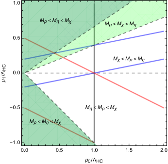
Figure 5: Mass hierarchy between $\rho$, $\chi$/$\omega$ and $\eta$ in the $\mu_{0}$–$\mu_{1}$ parameter space. The green regions are favourable for Dark Matter. The solid lines give, as a reference, the boundaries of the regions where $M_{\rho}<\Lambda_{\rm HC}$ (gray), $M_{\chi}=M_{\omega}<\Lambda_{\rm HC}$ (blue) and $M_{\eta}<\Lambda_{\rm HC}$ (red).

The mass spectrum of the $\Xi$ components in the $B$-preserving vacuum has been discussed in Sec. III.3: here we simply recall that

$$M_{\omega}=M_{\chi}\ =|\mu_{0}-5\mu_{1}|,\;\;M_{\rho}=\mu_{0}\;,$$ (110)

and the two iso-singlet hyper-fermions have the same mass as $\rho$, while $M_{\eta}=|\mu_{0}+2\mu_{1}|$ is correlated with the other two. As $\omega$ does not carry HC charges, it is crucial that it is not the lightest state. Furthermore, as $\eta$ is the only hyper-fermion in the fundamental of $Sp(4)_{\rm HC}$ that carries QCD color charges, mesons containing a single $\eta$ or $\tilde{\eta}$ are not good Dark Matter candidates. In the following, with the aim of presenting a qualilative discussion of the typical dark matter phenomenology, let us consider the case in which $\rho,\tilde{\rho}$ act as the dark matter candidate, with the typical parameter space for masses characterized by

$$M_{\rho}<M_{\omega}=M_{\chi}\,,\text{and}\,\,M_{\rho}<M_{\eta}$$ (111)

This configuration occurs in the light and dark green areas in Fig.5 in the $\mu_{0}$–$\mu_{1}$ parameter space. The light green wedge also features $M_{\chi}<M_{\eta}$, which could explain the lightness of leptons with respect to quarks in the same generation, C.f. Sec. III.5. As a final comment, bound states of $U_{t}$–$D_{b}$, if they receive a negative contribution to their mass from the binding energy, may also be lighter than $\rho$ and play the role of composite Dark Matter candidate. We also checked that all states with exotic $B$ charges can decay into $\rho$: for instance, $\omega\rightarrow\tilde{\rho}+t+\tau^{-}$, $\langle L_{u}^{3}\eta\rangle\rightarrow\rho+\bar{b}$, and so on. These may be very interesting final states to look for at the LHC or at future high energy hadron colliders.

A detailed study of the Dark Matter phenomenology of $\rho$ goes beyond the scope of this manuscript, and we leave it for further exploration. Yet, the most interesting property of this Dark Matter candidate is that it is stable thanks to the ordinary baryon numbers. Its relic density can, therefore, be linked to that of the ordinary baryons under some simple assumptions: a) a baryon or lepton asymmetry is generated at scales well above the EWSB scale (for instance, via leptogenesis Davidson:2008bu ); b) the EW phase transition is strong. Both conditions can be attained in the TPS model: the former via the presence of the heavy sterile neutrinos $N$, the latter thanks to the presence of additional light pNGBs accompanying the Higgs Bian:2019kmg ; DeCurtis:2019rxl . At the EW phase transition, therefore, the lepton or baryon asymmetries will be re-shuffled between the various active degrees of freedom in thermal equilibrium. The number of $\Xi$-components in the baryon asymmetry can then be computed following the procedure delineated in Ref. Harvey:1990qw (see also Refs Gudnason:2006yj ; Ryttov:2008xe ). In our case, the $\rho$ and $\omega$ are in thermal equilibrium thanks to the couplings to PC4F operators, which are enhanced at low energy by the anomalous dimensions, as it can be inferred, for instance, from the gauge-mediation currents in Eqs (41) and (42). More details on this calculation, and the assumptions adopted, are reported in the Appendix B. The final result is that the ratio of Dark Matter and baryon densities can be written as

$$\frac{\Omega_{\rm DM}}{\Omega_{b}}=\frac{M_{\rho}}{m_{N}}\left|2\sigma_{D}-2\sigma_{\eta}-5\sigma_{\chi}-\sigma_{\omega}\right|\,,$$ (112)

where $\sigma_{X}$ is a Boltzmann suppression factor which depends on the mass of the particle $X$ and the critical temperature $T_{\ast}$ of the EW phase transition, defined in Eq. (168).

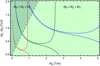
Figure 6: Points saturating the DM relic density in the $M_{\rho}$ vs. $M_{\chi}-M_{\rho}$ parameter space. The solid lines correspond to $T_{\ast}=246$ GeV (black), $T_{\ast}=100$ GeV (red) and $T_{\ast}=500$ GeV (blue).

In Fig. 6 we show the numerical result in the parameter region where $\rho$ is the lightest $\Xi$-component, focusing on the $\mu_{1}>0$ region (C.f. Fig. 5). We expressed the mass parameters $\mu_{0,1}$ in terms of $M_{\rho}$ and the mass difference $M_{\chi}-M_{\rho}$, where the dashed line corresponds to $M_{\eta}=M_{\chi}$ boundary. The black line corresponds to points saturating the Planck measurement Aghanim:2018eyx for $T_{\ast}=v_{\rm SM}=246$ GeV, showing that the $\rho$ mass is typically between $2.5\div 3$ TeV, except for a funnel region where cancellations between the Boltzmann factors occur. We also show results for $T_{\ast}=100$ GeV (red) and $T_{\ast}=500$ GeV (blue), showing how the $\rho$ mass can be lowered or enhanced. While these results are qualitative, they provide a reliable indication of the typical mass range for the components of the $\Xi$ multiplet, which also have consequences for the low energy properties of the composite theory. We see that the region with the mass hierarchy $M_{\rho}<M_{\chi}<M_{\eta}$, relevant in explaining the lightness of lepton masses, seems particularly favourable for this kind of Dark Matter candidate.

IV.5 Baryon Number Violation

Baryon number violation can occur in the TPS model in two ways: either via explicit interactions in the scalar potential, or via spontaneous breaking due to scalar VEVs.

As a example of the former, let’s consider the following quartic coupling:

$$\mathcal{L}_{V}\supset-\lambda_{4\Theta}\ \epsilon_{ijklmnop}\Theta^{ij*}\Theta^{kl*}\Theta^{mn*}\Theta^{op*}+\text{c.c.}$$ (113)

where $i,\dots,p$ are $SU(8)_{\rm PS}$ indices. This terms explicitly violates $U(1)_{G}$, thus it leads to baryon number violation. If we examine the decomposition of $\Theta$ at the HC level, we may identify two scalars with quantum numbers $\theta=(\textbf{1},\textbf{3})_{-1/3}$ and $\bar{\theta}=(\textbf{1},\bar{\textbf{3}})_{1/3}$, which coincides with the quantum number of one type of scalar leptoquark that can mediate proton decay Dorsner:2016wpm . However, while $\theta$ has $B_{\theta}=1/3$ and $L_{\theta}=1$, $\bar{\theta}$ has $B_{\bar{\theta}}=2/3$ and $L_{\bar{\theta}}=0$. Thus, the former behaves like a lepto-quark, while the latter as a di-quark:

$$\theta\rightarrow u+e^{-}\,,\quad\bar{\theta}\rightarrow u+d\,.$$ (114)

The coupling in Eq. (113), after $\Theta$ acquires a VEV, will however generate a mass mixing in the form $\lambda_{4\Theta}(v^{\Theta}_{\rm CHC})^{2}\theta\bar{\theta}$, thus allowing the standard proton decay operator

$$\frac{1}{M_{\theta}^{2}}(ud)(ue^{-})\,.$$ (115)

This kind of processes would require that the mass of these scalars is very large, $M_{\theta}\approx 10^{15\div 16}$ GeV.

The source of spontaneous $B$-violation is due to VEV(s) for the scalar multiplet $\Delta$, as shown in the bottom block of Table 7. This scenario has several interesting features, linked to mixing between the $\Xi$ components and other fermions and hyper-fermions, as discussed in Sec. III. However, it may also generate dangerous $B$ violating effects. One example is the presence of $B$-violating PC4F operators, mediated by scalars mixing $\Delta$ with other multiplets, as shown in Table 3. Such effects, while suppressed by a large scalar mass, may be enhanced at low energy by the anomalous running in the conformal phase, thus leaving sizeable traces at low energy. It may, therefore, not be enough to push the scalar masses and symmetry breaking scales above the proton decay limits.

IV.6 Final remarks

We have found that the TPS model can accommodate for masses and flavor mixing between the three SM generations, once it is suitably extended as shown in Table 6. The model can preserve baryon number, $B$, if the symmetry breaking is due to VEVs for $\Phi$, $\Psi$ and $\Theta^{1}$, while some couplings in the scalar potential are forbidden. This scenario also entails a candidate for Dark Matter, protected by a semi-integer baryon number.

One remarkable consequence of the TPS construction is that it fixes many essential properties of the model in the IR, i.e. in the confined phase. Besides the choice for the HC gauge group, this goes into the number of light hyper-fermions and their EW quantum numbers. For instance, we found that the low energy model resembles M8 of Belyaev:2016ftv , except for the hypercharge of $\chi$ (which is $-1/3$ in the TPS model, instead of $2/3$ Barnard:2013zea ; Ferretti:2013kya ). This difference implies that the low energy model suffers from corrections to the bottom couplings to the $Z$ boson Agashe:2006at , with strong bounds on the masses of the baryons as a consequence.

Furthermore, a detailed study of the low energy dynamics is crucial to establish the viability of the model in view of unwanted flavor and CP violation. This analysis is made more difficult by the ignorance of the dynamics in the walking phase, which can only be studied on the lattice: although the flavor scale is superheavy ($\Lambda_{F}\sim 10^{16}~{}{\mbox{GeV}}$), flavor-violation is incorporated into local PC4F operators whose effects are preserved down to $\Lambda_{HC}\sim 10~{}{\mbox{TeV}}$ due to large anomalous dimensions of certain hyperbaryon operators. The flavor-violating couplings are introduced due to the need to generate masses for the first and second family SM fermions, so we expect flavor violation is suppressed by light SM fermion Yukawas. However, it is known such suppression is not enough to be compatible with experimental bounds Panico:2015jxa . CP-violating couplings are also needed to generate the phase of CKM matrix in order to account for CP-violation phenomena in the quark sector. However, unwanted CP-violation may result in observables like electron electric dipole moment (EDM). Recent electron EDM results Andreev:2018ayy lead to strong constraint on the compositeness scale: $f\gtrsim 100~{}{\mbox{TeV}}$ where $f$ is the Goldstone decay constant Panico:2018hal . In the low-energy effective theory, introducing certain flavor symmetries may help relax the constraint Matsedonskyi:2014iha ; Frigerio:2018uwx . It could be tricky (if possible) to implement such symmetries in a UV-complete model like TPS, without affecting generating realistic masses and mixing of SM fermions. We therefore leave this issue for future study Giacomo:2019ehd .

V Summary and Outlook

That EWSB may originate from condensation in a new sector of strong dynamics is an attractive idea. Compared to the SM Higgs sector, which is parametrized via an elementary scalar field, it may naturally provide deeper insights into the possible origin of the EWSB and its connection to fermion mass generation. With the discovery of a $125~{}{\mbox{GeV}}$ Higgs-like particle and the need to accommodate the large top quark mass, it is then compelling to combine the idea of a pNGB Higgs and fermion partial compositeness in order to achieve natural and realistic models of EWSB based on strong dynamics.

In underlying gauge-fermion realisations, PC is realized via four-fermion operators built out of one SM fermion and three hyper-fermions charged under the new confining HC gauge group. In this work, we propose the first complete model, valid up to the Planck scale, that can generate the necessary four fermion operators (PC4F) in a model that has all the necessary features to provide a realistic low energy dynamics. This construction is based on the PUPC framework Cacciapaglia:2019dsq , where the HC and SM gauge symmetries are partially unified. When the larger gauge group undergoes spontaneous symmetry breaking, the resulting massive gauge bosons (and massive scalars) act as mediators for the PC4F operators.

Realizing the PUPC framework in practice, however, is highly non-trivial due to the many theoretical and phenomenological requirements. We found that the simplest model is based on an $SU(8)_{\rm PS}\times SU(2)_{L}\times SU(2)_{R}$ (TPS) gauge group, which breaks to an $Sp(4)_{\rm HC}$ and the SM gauge groups at a high scale $\Lambda_{\rm PU}\approx 10^{16}~{}{\mbox{GeV}}$. A minimal anomaly-free set of fermions can embed both the SM fermions and hyper-fermions needed to generate PC at low energy. Furthermore, we add suitable scalar fields at high scale (thus being natural) that play the roles of breaking the gauge group, generate PC4F operators via Yukawa couplings, and give masses to some hyper-fermions. The last feature is crucial in order to generate a walking dynamics between the UV unified phase and the IR confined one. We demonstrated that a renormalizable gauge-Yukawa theory based on the TPS gauge group automatically contains all the ingredients necessary to achieve the above goals. Thus, by a higher level unification we naturally achieve a tighter theoretical structure which gives deeper insight of the origin of fermion PC and mass generation.

In this work we have shown how the TPS model can generate masses for the three generations of SM fermions, with non-trivial mixing among them, while preserving all the attractive features of composite pNGB Higgs models. We identify several mechanisms that can explain the mass split between the various SM fermions (i.e., leptons versus quarks, bottom versus top) and the lightness of neutrinos via an inverse see-saw mechanism that arises naturally in this construction. Finally, the walking phase can be achieved by giving appropriate masses to the hyper-fermions appearing in the model. We pointed out that accidental $U(1)$ symmetries corresponding to the hyperbaryon number, the baryon number and the lepton number have important and interesting phenomenological consequences. In our TPS construction it is possible to preserve baryon number, thus avoiding strong constraints from proton and neutron decays, with the bonus feature of obtaining a Dark Matter candidate thanks to the presence of semi-integer baryon number neutral states. Under certain circumstances, the relic density can be linked to the baryon asymmetry, leading to typical masses for the Dark Matter candidate in the few TeV range.

While in this work we have proven the feasibility of the PUPC framework, via the explicit TPS realization, this work should be considered as a stepping stone to further investigate the phenomenology of the TPS model. The main points that need further investigations are:

• We have identified the minimal scalar sector and the phenomenologically relevant symmetry breaking patterns, due to scalar VEVs that are proven to exist in the literature. It is, nevertheless, necessary to check if the desired VEV patterns can be realized in the scalar potential of the complete model.

• The presence of a walking phase, where the theory approaches an IR conformal fixed point, is crucial for the realization of flavor physics in this model. While estimates seem to support the presence of such a phase in the TPS model, only lattice calculations can verify this non-perturbatively. Remarkably, in the TPS model both the gauge symmetry and the fermion properties are specified. Furthermore, calculating the anomalous dimensions of the hyper-baryon operators in this phase is crucial to understand the flavour structure at low energy.

• We have shown that the model can generate the needed flavor structures of the SM. A more detailed analysis is needed, however, to check if unwanted CP and flavor violating effects survive at low energy, which should face the strong experimental bounds. This analysis can be done in a reliable way only after lattice input is provided, in the form of anomalous dimensions in the walking phase to study the enhancement of flavor violating effects at low energy, and the spectrum of the baryons below the condensation scale.

• Finally, the running of the gauge couplings should be studied in detail, in order to check the consistency of partial unification, where the QCD and HC ones are the most relevant. This task is daring due to the fact that the HC dynamics is strong over many decades of energy, thus non-perturbative techniques are needed.

Although we do not attempt to solve these issues in the present work, we hope that our model-building effort can provide new perspectives for understanding and evaluating the pNGB Higgs and PC ideas, and motivate the community to investigate the related problems and the lattice community to explore uncharted territories that are crucial for our quest for mass generation.

Acknowledgements

CZ would like to thank Kingman Cheung, Jean-Pierre Derendinger and Xing-Bo Yuan for helpful discussions. GC and SV received partial support from the Labex-LIO (Lyon Institute of Origins) under grant ANR-10-LABX-66 (Agence Nationale pour la Recherche), and FRAMA (FR3127, Fédération de Recherche “André Marie Ampère”). GC and SV also acknowledge partial support from the LIA FCPPL (France-China Particle Physics Laboratory) and thank Sun Yat-Sen University, Guangzhou China, for hospitality during the early stages of this work.

Appendix A Field Decompositions

To match the TPS theory in the UV with the composite Higgs model in the IR, it is important to understand the decomposition of the TPS multiplets at various steps of the gauge symmetry breaking path. To this end, in this appendix we will provide for the reader all the necessary information, following the steps:

$$SU(8)_{\rm PS}\times SU(2)_{R}\rightarrow SU(7)_{\rm EHC}\times U(1)_{E}\rightarrow SU(4)_{\rm CHC}\times U(1)_{Y}\,,$$ (116)

where we omitted the $SU(2)_{L}$ gauge as it remains unbroken all the way down to the compositeness scale. Also, we recall that the additional $U(1)_{X}$ charges, relevant for the $\Psi$–$\Theta$ path, can be recovered as $Q_{X}=Q_{E}-Y$. Also, the $SU(4)_{\rm CHC}$ representations can be easily matched to the $Sp(4)_{\rm HC}$ ones as follows:

$${\bf 15}_{\rm CHC}\rightarrow{\bf 10}_{\rm HC}\oplus{\bf 5}_{\rm HC}\,,\quad{\bf 6}_{\rm CHC}\rightarrow{\bf 5}_{\rm HC}\oplus{\bf 1}_{\rm HC}\,,\quad{\bf 4/\bar{4}}_{\rm CHC}\rightarrow{\bf 4}_{\rm HC}\,.$$ (117)

To distinguish the components at various steps, we will use the following notation:

$$\{\textbf{56},\textbf{2}\}\Rightarrow\{SU(8)_{PS},SU(2)_{R})\},\quad\textbf{21}_{1/7}\Rightarrow SU(7)_{EHC,U(1)_{E}},\quad[\textbf{1},\bar{\textbf{3}}]_{1/3}\Rightarrow[SU(4)_{CHC},SU(3)_{C}]_{U(1)_{Y}}.$$ (118)

The decomposition of the $SU(2)_{L}$ and $SU(2)_{R}$ gauge bosons being rather straightforward, we will omit them and report the gauge multiplet of $SU(8)_{PS}$:

$$\{\textbf{63},\textbf{1}\}=\left\{\begin{array}[]{rcl}\textbf{1}_{0}&=&[\textbf{1},\textbf{1}]_{0}\\ \textbf{7}_{4/7}&=&[\textbf{1},\textbf{3}]_{2/3}\oplus[\textbf{4},\textbf{1}]_{1/2}\\ \bar{\textbf{7}}_{-4/7}&=&[\textbf{1},\bar{\textbf{3}}]_{-2/3}\oplus[\bar{\textbf{4}},\textbf{1}]_{-1/2}\\ \textbf{48}_{0}&=&[\textbf{1},\textbf{1}]_{0}\oplus[\textbf{4},\bar{\textbf{3}}]_{-1/6}\oplus[\bar{\textbf{4}},\textbf{3}]_{1/6}\oplus[\textbf{1},\textbf{8}]_{0}\oplus[\textbf{15},\textbf{1}]_{0}\end{array}\right.$$ (119)

For the scalar fields used in the model building, we have:

$$\Phi=\{\textbf{8},\textbf{2}\} = \left\{\begin{array}[]{rcl}\textbf{1}_{0}&=&[\textbf{1},\textbf{1}]_{0}\\ \textbf{1}_{-1}&=&[\textbf{1},\textbf{1}]_{-1}\\ \textbf{7}_{4/7}&=&[\textbf{1},\textbf{3}]_{2/3}\oplus[\textbf{4},\textbf{1}]_{1/2}\\ \textbf{7}_{-3/7}&=&[\textbf{1},\textbf{3}]_{-1/3}\oplus[\textbf{4},\textbf{1}]_{-1/2}\end{array}\right.$$ (124)

$$\Theta=\{\textbf{28},\textbf{1}\} = \left\{\begin{array}[]{rcl}\textbf{7}_{-3/7}&=&[\textbf{1},\textbf{3}]_{-1/3}\oplus[\textbf{4},\textbf{1}]_{-1/2}\\ \textbf{21}_{1/7}&=&[\textbf{1},\bar{\textbf{3}}]_{1/3}\oplus[\textbf{4},\textbf{3}]_{1/6}\oplus[\textbf{6},\textbf{1}]_{0}\end{array}\right.$$ (127)

$$\Delta=\{\textbf{56},\textbf{2}\} = \left\{\begin{array}[]{rcl}\textbf{21}_{1/7}&=&[\textbf{1},\bar{\textbf{3}}]_{1/3}\oplus[\textbf{4},\textbf{3}]_{1/6}\oplus[\textbf{6},\textbf{1}]_{0}\\ \textbf{21}_{-6/7}&=&[\textbf{1},\bar{\textbf{3}}]_{-2/3}\oplus[\textbf{4},\textbf{3}]_{-5/6}\oplus[\textbf{6},\textbf{1}]_{-1}\\ \textbf{35}_{5/7}&=&[\textbf{1},\textbf{1}]_{1}\oplus[\bar{\textbf{4}},\textbf{1}]_{1/2}\oplus[\textbf{4},\bar{\textbf{3}}]_{5/6}\oplus[\textbf{6},\textbf{3}]_{2/3}\\ \textbf{35}_{-2/7}&=&[\textbf{1},\textbf{1}]_{0}\oplus[\bar{\textbf{4}},\textbf{1}]_{-1/2}\oplus[\textbf{4},\bar{\textbf{3}}]_{-1/6}\oplus[\textbf{6},\textbf{3}]_{-1/3}\end{array}\right.$$ (132)

$$\Delta_{L}=\{\textbf{56},\textbf{1}\} = \left\{\begin{array}[]{rcl}\textbf{21}_{-5/14}&=&[\textbf{1},\bar{\textbf{3}}]_{-1/6}\oplus[\textbf{4},\textbf{3}]_{-1/3}\oplus[\textbf{6},\textbf{1}]_{-1/2}\\ \textbf{35}_{3/14}&=&[\textbf{1},\textbf{1}]_{1/2}\oplus[\bar{\textbf{4}},\textbf{1}]_{0}\oplus[\textbf{4},\bar{\textbf{3}}]_{1/3}\oplus[\textbf{6},\textbf{3}]_{1/6}\end{array}\right.$$ (135)

while for the adjoint $\Psi=\{\textbf{63},\textbf{1}\}$ the same decomposition as for the $SU(8)_{\rm PS}$ gauge bosons applies.

For the fermion multiplets used in the main text, we obtain

$$\Omega=\{\textbf{8},\textbf{1}\} = \left\{\begin{array}[]{rcl}\textbf{1}_{-1/2}&=&[\textbf{1},\textbf{1}]_{-1/2}\\ \textbf{7}_{-3/7}&=&[\textbf{1},\textbf{3}]_{1/6}\oplus[\textbf{4},\textbf{1}]_{0}\end{array}\right.$$ (138)

$$\Upsilon=\{\textbf{8},\textbf{2}\} = \left\{\begin{array}[]{rcl}\textbf{1}_{0}&=&[\textbf{1},\textbf{1}]_{0}\\ \textbf{1}_{-1}&=&[\textbf{1},\textbf{1}]_{-1}\\ \textbf{7}_{4/7}&=&[\textbf{1},\textbf{3}]_{2/3}\oplus[\textbf{4},\textbf{1}]_{1/2}\\ \textbf{7}_{-3/7}&=&[\textbf{1},\textbf{3}]_{-1/3}\oplus[\textbf{4},\textbf{1}]_{-1/2}\end{array}\right.$$ (143)

$$\Xi=\{\textbf{70},\textbf{1}\} = \left\{\begin{array}[]{rcl}\textbf{35}_{-2/7}&=&[\textbf{1},\textbf{1}]_{0}\oplus[\bar{\textbf{4}},\textbf{1}]_{-1/2}\oplus[\textbf{4},\bar{\textbf{3}}]_{-1/6}\oplus[\textbf{6},\textbf{3}]_{-1/3}\\ \bar{\textbf{35}}_{2/7}&=&[\textbf{1},\textbf{1}]_{0}\oplus[\textbf{4},\textbf{1}]_{1/2}\oplus[\bar{\textbf{4}},{\textbf{3}}]_{1/6}\oplus[\textbf{6},\bar{\textbf{3}}]_{1/3}\end{array}\right.$$ (146)

In principle, the multiplet $\Xi$ could be replaced by other anti-symmetric representations of $SU(8)_{\rm PS}$. We will briefly discuss the alternatives below.

A.1 2-index case

The fermion multiplet $\Xi$ coule be replaced by a two-index anti-symmetric $\Gamma_{2}$, and its conjugate $\bar{\Gamma}_{2}$, decomposing as

$$\Gamma_{2}=\{\textbf{28},\textbf{1}\} = \left\{\begin{array}[]{rcl}\textbf{7}_{-3/7}&=&[\textbf{1},\textbf{3}]_{-1/3}\oplus[\textbf{4},\textbf{1}]_{-1/2}\\ \textbf{21}_{1/7}&=&[\textbf{1},\bar{\textbf{3}}]_{1/3}\oplus[\textbf{4},\textbf{3}]_{1/6}\oplus[\textbf{6},\textbf{1}]_{0}\end{array}\right.$$ (149)

$$\bar{\Gamma}_{2}=\{\bar{\textbf{28}},\textbf{1}\} = \left\{\begin{array}[]{rcl}\bar{\textbf{7}}_{3/7}&=&[\textbf{1},\bar{\textbf{3}}]_{1/3}\oplus[\bar{\textbf{4}},\textbf{1}]_{1/2}\\ \bar{\textbf{21}}_{-1/7}&=&[\textbf{1},{\textbf{3}}]_{-1/3}\oplus[\bar{\textbf{4}},\bar{\textbf{3}}]_{-1/6}\oplus[\textbf{6},\textbf{1}]_{0}\end{array}\right.$$ (152)

Comparing with Eq. (146), we see that both contain iso-singlet hyper-fermions $D_{b}$ and $U_{t}$, QCD-colored hyper-fermions $\eta$–$\tilde{\eta}$, while the new fermions contain two copies of the bottom partners $\omega$–$\tilde{\omega}$. The main difference stands in the $\chi$-sector: for this choice, the $\chi$ has no QCD-colour charges. Thus, all the hyper-baryons coupling to quarks must contain $\eta$ or $\tilde{\eta}$, contrary to what we found in the TPS model with $\Xi$. Note also that the Yukawa couplings with $\Gamma_{2}$ would be different from the ones involving $\Xi$.

A.2 3-index case

Another alternative consists in using 3-index anti-symmetric representations, which will have the same decomposition as the scalars $\Delta$ and $\Delta_{L}$. In particular, we see from Eq. (135) that a singlet of the $SU(2)_{L/R}$ would contain a neutral iso-singlet hyper-fermion and a color-triplet with charge $1/6$, which is necessarily stable. To avoid this issue, the minimal option would be to promote the fermion $\Gamma_{3}$ to a doublet of $SU(2)_{R}$, thus having the same decomposition as $\Delta$:

$$\Gamma_{3}=\{\textbf{56},\textbf{2}\} = \left\{\begin{array}[]{rcl}\textbf{21}_{1/7}&=&[\textbf{1},\bar{\textbf{3}}]_{1/3}\oplus[\textbf{4},\textbf{3}]_{1/6}\oplus[\textbf{6},\textbf{1}]_{0}\\ \textbf{21}_{-6/7}&=&[\textbf{1},\bar{\textbf{3}}]_{-2/3}\oplus[\textbf{4},\textbf{3}]_{-5/6}\oplus[\textbf{6},\textbf{1}]_{-1}\\ \textbf{35}_{5/7}&=&[\textbf{1},\textbf{1}]_{1}\oplus[\bar{\textbf{4}},\textbf{1}]_{1/2}\oplus[\textbf{4},\bar{\textbf{3}}]_{5/6}\oplus[\textbf{6},\textbf{3}]_{2/3}\\ \textbf{35}_{-2/7}&=&[\textbf{1},\textbf{1}]_{0}\oplus[\bar{\textbf{4}},\textbf{1}]_{-1/2}\oplus[\textbf{4},\bar{\textbf{3}}]_{-1/6}\oplus[\textbf{6},\textbf{3}]_{-1/3}\end{array}\right.$$ (157)

$$\bar{\Gamma}_{3}=\{\bar{\textbf{56}},\textbf{2}\} = \left\{\begin{array}[]{rcl}\bar{\textbf{21}}_{-1/7}&=&[\textbf{1},{\textbf{3}}]_{-1/3}\oplus[\bar{\textbf{4}},\bar{\textbf{3}}]_{-1/6}\oplus[\textbf{6},\textbf{1}]_{0}\\ \bar{\textbf{21}}_{6/7}&=&[\textbf{1},{\textbf{3}}]_{2/3}\oplus[\bar{\textbf{4}},\bar{\textbf{3}}]_{5/6}\oplus[\textbf{6},\textbf{1}]_{1}\\ \bar{\textbf{35}}_{-5/7}&=&[\textbf{1},\textbf{1}]_{-1}\oplus[{\textbf{4}},\textbf{1}]_{-1/2}\oplus[\bar{\textbf{4}},{\textbf{3}}]_{-5/6}\oplus[\textbf{6},\bar{\textbf{3}}]_{-2/3}\\ \bar{\textbf{35}}_{2/7}&=&[\textbf{1},\textbf{1}]_{0}\oplus[{\textbf{4}},\textbf{1}]_{1/2}\oplus[\bar{\textbf{4}},{\textbf{3}}]_{1/6}\oplus[\textbf{6},\bar{\textbf{3}}]_{1/3}\end{array}\right.$$ (162)

The main drawback of this choice is that is contains a much larger number of hyper-fermions, thus seriously endangering the presence of a walking dynamics in the IR, C.f. sec. II.3.

Appendix B Dark Matter relic density calculation

SM + standard hyper-fermions						exotic $B$ fermions
		$Q$	$T_{L}^{3}$	$B$	$n_{f}$			$Q$	$T_{L}^{3}$	$B$	$n_{f}$
$t_{L}$	$\mu_{t_{L}}$	$2/3$	$1/2$	$1/3$	$9$	$U_{t}$	$-\mu_{D}$	$-1/2$	$0$	$-1/2$	$4$
$b_{L}$	$\mu_{b_{L}}$	$-1/3$	$-1/2$	$1/3$	$9$	$D_{b}$	$\mu_{D}$	$1/2$	$0$	$1/2$	$4$
$t_{R}^{c}$	$-\mu_{t_{R}}$	$-2/3$	$0$	$-1/3$	$9$	$\chi$	$\mu_{\chi}$	$-1/3$	$0$	$-1/6$	$15$
$b_{R}^{c}$	$-\mu_{b_{R}}$	$1/3$	$0$	$-1/3$	$9$	$\tilde{\chi}$	$-\mu_{\chi}$	$1/3$	$0$	$1/6$	$15$
$\nu_{L}$	$\mu_{\nu_{L}}$	$0$	$1/2$	$0$	$3$	$\eta$	$\mu_{\eta}$	$-1/6$	$0$	$1/6$	$12$
$\tau_{L}$	$\mu_{\tau_{L}}$	$-1$	$-1/2$	$0$	$3$	$\tilde{\eta}$	$-\mu_{\eta}$	$1/6$	$0$	$-1/6$	$12$
$\tau_{R}^{c}$	$-\mu_{\tau_{R}}$	$1$	$0$	$0$	$3$	$\omega$	$\mu_{\omega}$	$-1/3$	$0$	$-1/6$	$3$
$\nu_{R}^{c}$	$-\nu_{\nu_{R}}$	$0$	$0$	$0$	$3$	$\tilde{\omega}$	$-\mu_{\omega}$	$1/3$	$0$	$1/6$	$3$
$L_{u}^{3}$	$\mu_{L}$	$1/2$	$1/2$	$0$	$4$	$\rho$	$\mu_{\rho}$	$0$	$0$	$1/2$	$1$
$L_{d}^{3}$	$-\mu_{L}$	$-1/2$	$-1/2$	$0$	$4$	$\tilde{\rho}$	$\mu_{\rho}$	$0$	$0$	$-1/2$	$1$
$U_{d}^{3}$	$\mu_{U}$	$1/2$	$0$	$0$	$4$
$D_{u}^{3}$	$-\mu_{U}$	$-1/2$	$0$	$0$	$4$

Table 8: Weyl fermions participating to the EW phase transition; $n_{f}$ indicates the degrees of freedom of each spinor.

To compute how the baryon number generated above $\Lambda_{\rm HC}$ is transferred to the SM and to the fermions with fractional baryon number (components of $\Xi$), we consider only the states that have a mass below or around $\Lambda_{\rm HC}$. The fermions are listed in Table 8, with their electric charge $Q$, their weak iso-spin $T_{L}^{3}$, their baryon number $B$, and the multiplicity (which counts the gauge degrees of freedom). We already imposed the relation between the chemical potentials deriving from the hyper-fermion masses.

We shall also consider the $W^{\pm}$ gauge boson, for which we choose chemical potential $\mu_{W}$ associated to $W^{-}$ (and $-\mu_{W}$ for $W^{+}$). The EW interactions within the iso-doublets require:

$$\mu_{b_{L}}=\mu_{t_{L}}+\mu_{W}\,,\quad\mu_{\tau_{L}}=\mu_{\nu_{L}}+\mu_{W}\,,\quad\mu_{L}=-\frac{1}{2}\mu_{W}\,.$$ (163)

To take into account the HC dynamics, which replaces the Higgs sector of the SM, we include in the counting of degrees of freedom the hyper-fermions themselves. This is a rough approximation, as the EW phase transition may occur below the condensation scale, where it would be more appropriate to consider bound states. Nevertheless, as we want to obtain a rough estimate of the Dark Matter mass, to simplify the analysis we will stay within this approximation.

Additional relations between the chemical potentials derive from the PC4F operators that survive at low energy due to the large anomalous dimension enhancement. To simplify the analysis, again, we will only consider gauge-mediated PC4F operators. Looking at the expression of the currents in Eqs (41) and (42), we see that the $\Xi$-components $\rho$ and $\omega$ also participate to PC. Thus, considering the PC4F operators is equivalent to imposing the equality of the chemical potentials of the various components of the currents, namely for $J_{E}^{\mu}$:

$$-\mu_{t_{L}}+\mu_{L}=\mu_{U}-\mu_{t_{R}}=-\mu_{U}-\mu_{b_{R}}=-\mu_{\chi}-\mu_{D}=-\mu_{\eta}+\mu_{\chi}=-\mu_{\eta}+\mu_{\omega}=-\mu_{\rho}+\mu_{\eta}=-\mu_{\omega}-\mu_{D}\,;$$ (164)

while for $J_{C}^{\mu}$:

$$\mu_{L}+\mu_{\tau_{L}}=\mu_{\nu_{R}}-\mu_{U}=\mu_{\tau_{R}}+\mu_{U}=\mu_{\eta}+\mu_{\chi}=\mu_{\eta}+\mu_{\omega}=\mu_{\rho}-\mu_{D}\,.$$ (165)

The relations above allow to determine all the chemical potentials but 4.

A phase transition of the 1st order is characterized by the vanishing of the total electric charge and iso-spin, given by

$$Q_{\rm tot}=9\left[\frac{2}{3}(\mu_{t_{L}}+\mu_{t_{R}})-\frac{1}{3}(\mu_{b_{L}}+\mu_{b_{R}})\right]+3\left[-(\mu_{\tau_{L}}+\mu_{\tau_{R}})\right]+4\left[\frac{1}{2}\mu_{L}2\sigma_{L}+\frac{1}{2}\mu_{U}2\sigma_{U}+\frac{1}{2}\mu_{D}2\sigma_{D}\right]+\\ 15\left(-\frac{1}{3}\mu_{\chi}\right)2\sigma_{\chi}+12\left(-\frac{1}{6}\mu_{\eta}\right)2\sigma_{\eta}+3\left(-\frac{1}{3}\mu_{\omega}\right)2\sigma_{\omega}+4(-\mu_{W})\,,$$ (166)

$$T^{3}_{\rm tot}=\frac{1}{2}\left[9(\mu_{t_{L}}-\mu_{b_{L}})+3(\mu_{\nu_{L}}-\mu_{\tau_{R}})+4\mu_{L}2\sigma_{L}\right]-4\mu_{W}\,,$$ (167)

where we have introduced the statistical factor for fermions

$$\sigma_{X}=\frac{3}{2\pi^{2}}\int_{0}^{\infty}dx\;x^{2}\cosh^{-2}\left(\frac{1}{2}\sqrt{x^{2}+z^{2}}\right)\,,\qquad z=\frac{m_{X}}{T}\,,$$ (168)

$T$ being the temperature. The conditions $Q_{\rm tot}=0$ and $T^{3}_{\rm tot}=0$, together with the EW Sphaleron condition

$$\mu_{t_{L}}+2\mu_{b_{L}}+\mu_{\nu_{L}}=0\,,$$ (169)

allow to fix all chemical potentials as a function of one.

Finally, the baryon number density in the SM quarks (which corresponds after the EW phase transition to the net baryon number density in the Universe), can be expressed as

$$n_{b}^{\rm SM}=-\frac{12(3+\sigma_{U})}{6+3\sigma_{D}+\sigma_{\eta}+5\sigma_{\chi}+\sigma_{\omega}}\mu_{U}\,,$$ (170)

while the total number density of fermions in the $\xi$–components is

$$n_{\Xi}=-\frac{12(3+\sigma_{U})(2\sigma_{D}-2\sigma_{\eta}-5\sigma_{\chi}-\sigma_{\omega})}{6+3\sigma_{D}+\sigma_{\eta}+5\sigma_{\chi}+\sigma_{\omega}}\mu_{U}=(2\sigma_{D}-2\sigma_{\eta}-5\sigma_{\chi}-\sigma_{\omega})n_{b}^{\rm SM}\,.$$ (171)

Finally, we can express the relic density of Dark Matter, divided by the baryon density, as

$$\frac{\Omega_{\rm DM}}{\Omega_{b}}=\frac{M_{\rho}}{m_{N}}\left|\frac{n_{\Xi}}{n_{b}^{\rm SM}}\right|=|2\sigma_{D}-2\sigma_{\eta}-5\sigma_{\chi}-\sigma_{\omega}|\frac{M_{\rho}}{m_{N}}=5.36\,,$$ (172)

where $m_{N}\approx 1$ GeV is the nucleon mass, and the numerical value comes from the Planck 2018 measurement Aghanim:2018eyx . The equation above can be used to determine the mass of the Dark Matter, $M_{\rho}$, as a function of the temperature of the EW phase transition (which enters in the expressions for the $\sigma$-functions).

References

- (1) S. L. Glashow, Nucl. Phys. 22, 579 (1961).
- (2) S. Weinberg, Phys. Rev. Lett. 19, 1264 (1967).
- (3) A. Salam, Conf. Proc. C680519, 367 (1968).
- (4) ATLAS, G. Aad et al., Phys. Lett. B716, 1 (2012), 1207.7214.
- (5) CMS, S. Chatrchyan et al., Phys. Lett. B716, 30 (2012), 1207.7235.
- (6) R. Barbieri, A. Pomarol, R. Rattazzi, and A. Strumia, Nucl. Phys. B703, 127 (2004), hep-ph/0405040.
- (7) F. Englert and R. Brout, Phys. Rev. Lett. 13, 321 (1964).
- (8) P. W. Higgs, Phys. Lett. 12, 132 (1964).
- (9) P. W. Higgs, Phys. Rev. Lett. 13, 508 (1964).
- (10) G. S. Guralnik, C. R. Hagen, and T. W. B. Kibble, Phys. Rev. Lett. 13, 585 (1964).
- (11) ATLAS, CMS, G. Aad et al., JHEP 08, 045 (2016), 1606.02266.
- (12) M. Cepeda et al.Report from Working Group 2: Higgs Physics at the HL-LHC and HE-LHC Vol. 7 (, 2019), pp. 221–584, 1902.00134.
- (13) S. Weinberg, Phys. Rev. D13, 974 (1976), [Addendum: Phys. Rev.D19,1277(1979)].
- (14) S. Dimopoulos and L. Susskind, 2, 930 (1979).
- (15) E. Eichten and K. D. Lane, Phys. Lett. 90B, 125 (1980).
- (16) D. B. Kaplan and H. Georgi, Phys. Lett. 136B, 183 (1984).
- (17) R. Barbieri and A. Strumia, The ’LEP paradox’, in 4th Rencontres du Vietnam: Physics at Extreme Energies (Particle Physics and Astrophysics) Hanoi, Vietnam, July 19-25, 2000, 2000, hep-ph/0007265.
- (18) B. Holdom, Phys. Rev. D24, 1441 (1981).
- (19) D. B. Kaplan, Nucl. Phys. B365, 259 (1991).
- (20) A. G. Cohen and H. Georgi, Nucl. Phys. B314, 7 (1989).
- (21) R. Contino, Y. Nomura, and A. Pomarol, Nucl. Phys. B671, 148 (2003), hep-ph/0306259.
- (22) Y. Hosotani and M. Mabe, Phys. Lett. B615, 257 (2005), hep-ph/0503020.
- (23) K. Agashe, R. Contino, and A. Pomarol, Nucl. Phys. B719, 165 (2005), hep-ph/0412089.
- (24) K. Agashe and R. Contino, Nucl. Phys. B742, 59 (2006), hep-ph/0510164.
- (25) R. Contino, The Higgs as a Composite Nambu-Goldstone Boson, in Physics of the large and the small, TASI 09, proceedings of the Theoretical Advanced Study Institute in Elementary Particle Physics, Boulder, Colorado, USA, 1-26 June 2009, pp. 235–306, 2011, 1005.4269.
- (26) B. Bellazzini, C. Csaki, and J. Serra, Eur. Phys. J. C74, 2766 (2014), 1401.2457.
- (27) G. Panico and A. Wulzer, Lect. Notes Phys. 913, pp.1 (2016), 1506.01961.
- (28) G. Cacciapaglia, C. Pica, and F. Sannino, (2020), 2002.04914.
- (29) O. Matsedonskyi, JHEP 02, 154 (2015), 1411.4638.
- (30) G. Cacciapaglia et al., JHEP 06, 085 (2015), 1501.03818.
- (31) G. Panico and A. Pomarol, JHEP 07, 097 (2016), 1603.06609.
- (32) K. Agashe, R. Contino, and R. Sundrum, Phys. Rev. Lett. 95, 171804 (2005), hep-ph/0502222.
- (33) J. M. Maldacena, Int. J. Theor. Phys. 38, 1113 (1999), hep-th/9711200, [Adv. Theor. Math. Phys.2,231(1998)].
- (34) J. Erlich, E. Katz, D. T. Son, and M. A. Stephanov, Phys. Rev. Lett. 95, 261602 (2005), hep-ph/0501128.
- (35) L. Da Rold and A. Pomarol, Nucl. Phys. B 721, 79 (2005), hep-ph/0501218.
- (36) J. Hirn and V. Sanz, JHEP 12, 030 (2005), hep-ph/0507049.
- (37) F. Caracciolo, A. Parolini, and M. Serone, JHEP 02, 066 (2013), 1211.7290.
- (38) D. Marzocca, A. Parolini, and M. Serone, JHEP 03, 099 (2014), 1312.5664.
- (39) H. Gies, Phys. Rev. D68, 085015 (2003), hep-th/0305208.
- (40) T. R. Morris, JHEP 01, 002 (2005), hep-ph/0410142.
- (41) J. Barnard, T. Gherghetta, and T. S. Ray, JHEP 02, 002 (2014), 1311.6562.
- (42) G. Ferretti and D. Karateev, JHEP 03, 077 (2014), 1312.5330.
- (43) L. Vecchi, JHEP 02, 094 (2017), 1506.00623.
- (44) G. Ferretti, JHEP 06, 107 (2016), 1604.06467.
- (45) A. Belyaev et al., JHEP 01, 094 (2017), 1610.06591, [Erratum: JHEP12,088(2017)].
- (46) T. DeGrand, Rev. Mod. Phys. 88, 015001 (2016), 1510.05018.
- (47) E. Bennett et al., JHEP 03, 185 (2018), 1712.04220.
- (48) V. Ayyar et al., Phys. Rev. D97, 114505 (2018), 1801.05809.
- (49) V. Ayyar et al., Phys. Rev. D99, 094502 (2019), 1812.02727.
- (50) Bennett et al., (2019), 1909.12662.
- (51) A. Hasenfratz, C. Rebbi, and O. Witzel, Phys. Lett. B773, 86 (2017), 1609.01401.
- (52) F. Sannino, A. Strumia, A. Tesi, and E. Vigiani, JHEP 11, 029 (2016), 1607.01659.
- (53) G. Cacciapaglia, H. Gertov, F. Sannino, and A. E. Thomsen, Phys. Rev. D98, 015006 (2018), 1704.07845.
- (54) F. Sannino, P. Stangl, D. M. Straub, and A. E. Thomsen, Phys. Rev. D97, 115046 (2018), 1712.07646.
- (55) S. Samuel, Nucl. Phys. B347, 625 (1990).
- (56) J. Galloway, A. L. Kagan, and A. Martin, Phys. Rev. D95, 035038 (2017), 1609.05883.
- (57) A. Agugliaro, O. Antipin, D. Becciolini, S. De Curtis, and M. Redi, Phys. Rev. D95, 035019 (2017), 1609.07122.
- (58) C. T. Hill and E. H. Simmons, Phys. Rept. 381, 235 (2003), hep-ph/0203079, [Erratum: Phys. Rept.390,553(2004)].
- (59) T. Appelquist and R. Shrock, Phys. Rev. Lett. 90, 201801 (2003), hep-ph/0301108.
- (60) T. Appelquist, M. Piai, and R. Shrock, Phys. Rev. D69, 015002 (2004), hep-ph/0308061.
- (61) T. Appelquist, N. D. Christensen, M. Piai, and R. Shrock, Phys. Rev. D70, 093010 (2004), hep-ph/0409035.
- (62) G. Cacciapaglia, S. Vatani, and Z.-W. Wang, (2019), 1909.08628.
- (63) O. Antipin and F. Sannino, Phys. Rev. D97, 116007 (2018), 1709.02354.
- (64) G. Cacciapaglia, S. Vatani, T. Ma, and Y. Wu, (2018), 1812.04005.
- (65) G. Cacciapaglia, S. Vatani, and C. Zhang, (2019), 1911.05454.
- (66) N. Cabibbo, Phys. Rev. Lett. 10, 531 (1963).
- (67) M. Kobayashi and T. Maskawa, Prog. Theor. Phys. 49, 652 (1973).
- (68) Z. Maki, M. Nakagawa, and S. Sakata, Prog. Theor. Phys. 28, 870 (1962).
- (69) D. D. Dietrich and F. Sannino, Phys. Rev. D 75, 085018 (2007), hep-ph/0611341.
- (70) F. Sannino, Phys. Rev. D 79, 096007 (2009), 0902.3494.
- (71) T. A. Ryttov and F. Sannino, Int. J. Mod. Phys. A 25, 4603 (2010), 0906.0307.
- (72) M. Mojaza, C. Pica, T. A. Ryttov, and F. Sannino, Phys. Rev. D 86, 076012 (2012), 1206.2652.
- (73) J. C. Pati and A. Salam, Phys. Rev. D10, 275 (1974), [Erratum: Phys. Rev.D11,703(1975)].
- (74) L.-F. Li, Phys. Rev. D 9, 1723 (1974).
- (75) V. Elias, S. Eliezer, and A. Swift, Phys. Rev. D 12, 3356 (1975).
- (76) F. Buccella, H. Ruegg, and C. A. Savoy, Nucl. Phys. B 169, 68 (1980).
- (77) H. Ruegg, Phys. Rev. D 22, 2040 (1980).
- (78) C. Cummins and R. King, J. Phys. A 17, L627 (1984).
- (79) S. L. Adler, Phys. Lett. B 744, 380 (2015), 1503.07084.
- (80) C. Pica and F. Sannino, Phys. Rev. D83, 116001 (2011), 1011.3832.
- (81) F. Sannino, Acta Phys. Polon. B40, 3533 (2009), 0911.0931.
- (82) F. Lyonnet, I. Schienbein, F. Staub, and A. Wingerter, Comput. Phys. Commun. 185, 1130 (2014), 1309.7030.
- (83) F. Lyonnet and I. Schienbein, Comput. Phys. Commun. 213, 181 (2017), 1608.07274.
- (84) A. Eichhorn, Front. Astron. Space Sci. 5, 47 (2019), 1810.07615.
- (85) M. Golterman and Y. Shamir, Phys. Rev. D91, 094506 (2015), 1502.00390.
- (86) M. A. Shifman, A. I. Vainshtein, and V. I. Zakharov, Nucl. Phys. B147, 385 (1979).
- (87) M. A. Shifman, A. I. Vainshtein, and V. I. Zakharov, Nucl. Phys. B147, 448 (1979).
- (88) J. Galloway, J. A. Evans, M. A. Luty, and R. A. Tacchi, JHEP 10, 086 (2010), 1001.1361.
- (89) G. Cacciapaglia and F. Sannino, JHEP 04, 111 (2014), 1402.0233.
- (90) C. Cai, G. Cacciapaglia, and H.-H. Zhang, JHEP 01, 130 (2019), 1805.07619.
- (91) G. Cacciapaglia, S. Vatani, and C. Zhang, in preparation.
- (92) M. Rosenlyst and C. T. Hill, Phys. Rev. D 101, 095027 (2020), 2002.04931.
- (93) G. C. Branco et al., Phys. Rept. 516, 1 (2012), 1106.0034.
- (94) R. Volkas, Phys. Rev. D 53, 2681 (1996), hep-ph/9507215.
- (95) A. Abada and M. Lucente, Nucl. Phys. B885, 651 (2014), 1401.1507.
- (96) D. Marzocca, M. Serone, and J. Shu, JHEP 08, 013 (2012), 1205.0770.
- (97) E. Eichten and B. R. Hill, Phys. Lett. B 234, 511 (1990).
- (98) H. Georgi, Phys. Lett. B 240, 447 (1990).
- (99) D. Buarque Franzosi and G. Ferretti, SciPost Phys. 7, 027 (2019), 1905.08273.
- (100) K. Agashe and R. Contino, Phys. Rev. D 80, 075016 (2009), 0906.1542.
- (101) A. Carmona and F. Goertz, JHEP 04, 163 (2013), 1301.5856.
- (102) A. Carmona and F. Goertz, Phys. Rev. Lett. 116, 251801 (2016), 1510.07658.
- (103) M. Frigerio, M. Nardecchia, J. Serra, and L. Vecchi, JHEP 10, 017 (2018), 1807.04279.
- (104) G. Cacciapaglia et al., JHEP 04, 006 (2008), 0709.1714.
- (105) A. Fitzpatrick, G. Perez, and L. Randall, Phys. Rev. Lett. 100, 171604 (2008), 0710.1869.
- (106) C. Csaki, A. Falkowski, and A. Weiler, JHEP 09, 008 (2008), 0804.1954.
- (107) R. A. Porto and A. Zee, Phys. Lett. B 666, 491 (2008), 0712.0448.
- (108) J. Preskill and S. Weinberg, Phys. Rev. D24, 1059 (1981).
- (109) S. Weinberg, The quantum theory of fields. Vol. 2: Modern applications (Cambridge University Press, 2013).
- (110) C. Vafa and E. Witten, Nucl. Phys. B234, 173 (1984).
- (111) R. N. Mohapatra and R. E. Marshak, Phys. Rev. Lett. 44, 1316 (1980), [Erratum: Phys. Rev. Lett.44,1643(1980)].
- (112) L. Di Luzio, Aspects of symmetry breaking in Grand Unified Theories, PhD thesis, SISSA, Trieste, 2011, 1110.3210.
- (113) S. Davidson, E. Nardi, and Y. Nir, Phys. Rept. 466, 105 (2008), 0802.2962.
- (114) L. Bian, Y. Wu, and K.-P. Xie, JHEP 12, 028 (2019), 1909.02014.
- (115) S. De Curtis, L. Delle Rose, and G. Panico, JHEP 12, 149 (2019), 1909.07894.
- (116) J. A. Harvey and M. S. Turner, Phys. Rev. D 42, 3344 (1990).
- (117) S. B. Gudnason, C. Kouvaris, and F. Sannino, Phys. Rev. D74, 095008 (2006), hep-ph/0608055.
- (118) T. A. Ryttov and F. Sannino, Phys. Rev. D 78, 115010 (2008), 0809.0713.
- (119) Planck, N. Aghanim et al., (2018), 1807.06209.
- (120) I. Dorsner, S. Fajfer, A. Greljo, J. F. Kamenik, and N. Kosnik, Phys. Rept. 641, 1 (2016), 1603.04993.
- (121) K. Agashe, R. Contino, L. Da Rold, and A. Pomarol, Phys. Lett. B 641, 62 (2006), hep-ph/0605341.
- (122) ACME, V. Andreev et al., Nature 562, 355 (2018).
- (123) G. Panico, A. Pomarol, and M. Riembau, JHEP 04, 090 (2019), 1810.09413.