NLO QCD+NLO EW corrections to diboson production matched to parton shower

Abstract

We present the matching of NLO QCD and NLO EW corrections to parton showers for vector-boson pair production at the LHC. We consider leptonic final states, including resonant and non-resonant diagrams, spin correlations and off-shell effects. Our results are obtained interfacing the Recola2-Collier one-loop provider with the POWHEG-BOX-RES framework. We discuss our implementation, we validate it at fixed order, and we show our final results matched to parton shower. A by-product of our work is also a general interface between Recola2-Collier and POWHEG-BOX-RES. This is the first time that EW and QCD corrections to diboson production are consistently matched to parton showers.

1 Introduction

The pair production of massive vector bosons at the LHC ($pp\to VV^{\prime}$, with $VV^{\prime}=\{W^{+}W^{-}$, $ZZ$, $W^{\pm}Z\}$) is among the most studied Standard Model (SM) processes, both as a signal on its own and as a background to physics beyond the Standard Model (BSM) and Higgs searches. Electroweak boson pair production involving at least a $W$ boson in the final state ($W^{+}W^{-}$ and $ZW^{\pm}$) is important for collider phenomenology because it is sensitive to the $ZWW$ gauge-boson self interaction, and therefore precision measurements of $VV^{\prime}$ processes provide a test of the electroweak gauge structure. These precision tests are usually carried out by setting bounds on the allowed size of anomalous trilinear gauge couplings (aTGCs) [1], although several other ideas have been proposed to study effects due to BSM physics with $VV$ final states [2, 3, 4, 5, 6, 7, 8, 9, 10, 11, 12, 13]. Diboson production is also a background for several searches, notably those involving an heavy resonance decaying to a pair of gauge bosons. In particular, $pp\to W^{+}W^{-}$ and $pp\to ZZ$ are irreducible background for Higgs production, when the Higgs boson decays to gauge bosons.

For all the above reasons, it is essential to make accurate predictions for vector boson pair production processes. Among the possible final states, the one where four leptons are present is probably the most interesting one, as it allows precise measurements, due to its clear signature. In the rest of this work, including this section, we will only discuss final states with four leptons, although we will often use the $VV^{\prime}$ intermediate state as a shorthand notation to identify the full process. We will give more details on the exact leptonic final state, and approximations made, only where needed.

The status of predictions at fixed-order in the strong ($\alpha_{\mathchoice{\displaystyle}{\scriptstyle}{\scriptscriptstyle}{\scriptscriptstyle}\rm S}$) and/or electroweak ($\alpha$) coupling for diboson production with leptonic decays is rather advanced. As far as QCD corrections are concerned, the next-to-leading-order (NLO) QCD corrections for the process $q\bar{q}^{(\prime)}\to VV^{\prime}$ (with leptonic decays, interference and off-shell effects fully taken into account) were obtained in Refs. [14, 15, 16, 17]. The NNLO QCD corrections were computed more recently, in Refs. [18, 19, 20, 21, 22, 23]. The loop-induced processes $gg\to W^{+}W^{-}$ and $gg\to ZZ$ contribute to the final state at the same order in $\alpha_{\mathchoice{\displaystyle}{\scriptstyle}{\scriptscriptstyle}{\scriptscriptstyle}\rm S}$ as the NNLO corrections to the $q\bar{q}$ initial state. They have been computed at LO in Refs. [25, 26, 27], and the relative NLO corrections ($\mathcal{O}(\alpha_{\mathchoice{\displaystyle}{\scriptstyle}{\scriptscriptstyle}{\scriptscriptstyle}\rm S}^{3})$) were obtained more recently, in Refs. [28, 29, 30, 31].

Although electroweak (EW) corrections are usually small for total cross sections, they can have an impact on differential distributions. Typically this is the case for large invariant-mass or transverse-momentum ($p_{\mathchoice{\displaystyle}{\scriptstyle}{\scriptscriptstyle}{\scriptscriptstyle}\rm T}$) distributions, due to the so-called EW Sudakov logarithms. Sizeable effects due to radiative photons are also visible, for leptonic observables, near resonances or kinematic thresholds. NLO EW corrections to the $q\bar{q}^{(\prime)}\to VV^{\prime}$ processes (with leptonic decays and interference effects) were computed in Ref. [32, 33, 34, 35, 36], improving on the results obtained for stable vector bosons in [37, 38, 39]. For on-shell $W^{+}W^{-}$ production, subleading EW Sudakov corrections at next-to-next-to-leading logarithmic (NNLL) accuracy were considered in Ref. [40].

In the context of all-order computations in QCD, the NNLL-accurate results for the transverse-momentum distribution of the leptonic final state arising from $pp\to VV^{\prime}$ production were obtained in Ref. [41, 42, 43], whereas jet-veto logarithms were resummed at NNLL in Ref. [44, 45, 46]. All these resummed results were matched to the inclusive NLO (or NNLO) total cross sections. The most accurate predictions were obtained in Ref. [47]: the transverse momentum of the $W^{+}W^{-}$ system was resummed at NNLO+N3LL accuracy, the jet-veto logarithms were resummed at NNLO+NNLL, and a joint resummation for the $W^{+}W^{-}$ $p_{\mathchoice{\displaystyle}{\scriptstyle}{\scriptscriptstyle}{\scriptscriptstyle}\rm T}$ spectrum in presence of a jet veto was performed at NNLO+NNLL.

The matching of fixed-order computations in QCD with parton showers (PS) algorithms (NLO-QCD+PS) is well established with the MC@NLO [48] and the POWHEG [49, 50] matching algorithms, that are implemented in the public software MadGraph5_aMC@NLO [51] and POWHEG-BOX [52]. Variants of these algorithms are also available within the Sherpa generator [53, 54] and in Herwig7 [55], through the MatchBox framework [56]. Dedicated studies of $pp\to VV^{\prime}$ production at NLO-QCD+PS, with full leptonic decays and including resonant and non-resonant diagrams as well as spin correlations and off-shell effects exactly, were performed in Ref. [57, 58, 59, 60, 61, 10, 11]. Notably, starting from the NLO+PS merging of $pp\to W^{+}W^{-}$ and $pp\to W^{+}W^{-}+j$ [62] obtained through the MiNLO approach [63], NNLO-QCD+PS results for the $pp\to W^{+}W^{-}$ process were obtained in Ref. [64].

As far as the combination of QCD and EW results at fixed-order is concerned, this has been studied at NLO QCD + NLO EW accuracy in Ref. [36], and more recently, at NNLO QCD + NLO EW in Ref. [65].

In this work we combine the NLO QCD corrections and the NLO EW ones, and match them to parton shower for the first time. Our underlying NLO computation is performed combining the exact $\mathcal{O}(\alpha_{\mathchoice{\displaystyle}{\scriptstyle}{\scriptscriptstyle}{\scriptscriptstyle}\rm S})$ and the exact $\mathcal{O}(\alpha)$ effects in an additive way, and it is matched to a complete PS algorithm where both QCD and QED emissions are simulated. We will discuss how the matching is performed in Sect. 2. Here we stress that our results are the first ones where the matching is achieved exactly for diboson production. In previous publications, as, for instance, for some of the results presented in Ref. [36], QED corrections were included only via the PS, after having subtracted from the hard matrix elements, and in an approximate manner, the QED effects due to radiative photon emission, while keeping the Sudakov logarithms of pure weak origin, arising from virtual $W$ and $Z$ boson exchange. More recently, the same approximation was used by the authors of Ref. [67], where a NLO-QCD+PS merging of the $pp\to W^{+}W^{-}$ and $pp\to W^{+}W^{-}+j$ processes was achieved keeping weak corrections and approximate QED effects.

We also remind the reader that, at fixed-order, a description of mixed terms can be obtained via a factorized ansatz, i.e. multiplying differential NLO QCD cross sections by EW correction factors, as done, for instance, in Ref. [36]. In our approach, mixed $\mathcal{O}(\alpha_{\mathchoice{\displaystyle}{\scriptstyle}{\scriptscriptstyle}{\scriptscriptstyle}\rm S}^{n}\alpha^{m})$ terms are generated through the exponentiation of QED and QCD radiation in the POWHEG Sudakov form factor, and the mixed terms generated in this way are then only correct in the QCD and QED collinear limits.

The paper is organized as follows: in Sect. 2 we describe the details of our computation, in Sect. 3 we list the parameters and cuts used throughout this work, and in Sect. 4 we discuss the validation of our implementation. In Sect. 5 we show a selection of the new results, i.e. the matching of NLO EW + NLO QCD corrections to parton shower. We summarize our work in Sect. 6.

In the rest of this manuscript we will use the shorthand $\rm NLO_{\rm QCD}$ and $\rm NLO_{\rm EW}$ to denote NLO accuracy in the $\alpha_{\mathchoice{\displaystyle}{\scriptstyle}{\scriptscriptstyle}{\scriptscriptstyle}\rm S}$ and $\alpha$ perturbative expansion, respectively. We use the notation $\rm NLO_{\rm QCD}$ + $\rm NLO_{\rm EW}$ to denote the additive combination of the hard matrix elements (in the POWHEG $\bar{B}$ function).

2 Details of the calculation

In this paper we consider the processes

$$pp \to e^{+}\nu_{e}\mu^{-}\overline{\nu}_{\mu}\,,$$

$$pp \to \mu^{+}\nu_{\mu}e^{-}e^{+}\,,$$

$$pp \to \mu^{+}\mu^{-}e^{-}e^{+}\,.$$ (1)

We stress that the full matrix elements for four fermion production are used and no on-shell or double pole approximation is employed. In the following the three processes will be dubbed as $WW$, $WZ$, and $ZZ$ production, and, collectively, as “diboson production”. Although we will show results only for $W^{+}Z$ production, our code is fully general and $W^{-}Z$ production can be generated as well.

                         

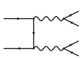
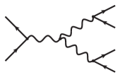
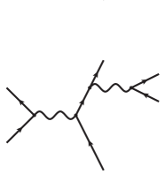
Figure 1: Representative Feynman diagrams for the possible classes of resonance histories contributing at LO.

The calculation of the $\rm NLO_{\rm QCD}$ + $\rm NLO_{\rm EW}$ corrections to diboson production matched to QCD and QED parton shower presented in this paper is performed in the POWHEG-BOX-RES framework [68], which is a framework designed to simulate processes involving intermediate decaying resonances with NLO+PS accuracy. It is a new implementation of the POWHEG method [49, 50] that overcomes the limitations of the POWHEG-BOX framework [52]. It has been used in Ref. [69] to simulate the process $pp\to b\bar{b}\ell\bar{\ell}\nu\bar{\nu}$ with $\rm NLO_{\rm QCD}$+PS accuracy, thereby achieving, for the first time, a fully-consistent treatment of $t\bar{t}$ and $Wt$ production with two leptonic decays, in Ref. [70] to compute the processes $pp\to HV$ and $pp\to HVj$ production ($V=W,Z$) with $\rm NLO_{\rm QCD}$ + $\rm NLO_{\rm EW}$+PS accuracy, and in Ref. [71] to compute the $\rm NLO_{\rm EW}$+PS corrections to $pp\to\ell\ell^{\prime}\nu\nu^{\prime}jj$. In Ref. [72], a simplified version of the POWHEG-BOX-RES algorithm has been implemented also in the W_ew-BMNNP and Z_ew-BMNNPV packages [73, 74, 72, 75] of POWHEG-BOX-V2, in order to simulate neutral and charged Drell-Yan production with $\rm NLO_{\rm QCD}$ + $\rm NLO_{\rm EW}$+PS accuracy in a fully-consistent manner. A fully independent calculation of $\rm NLO_{\rm QCD}$ + $\rm NLO_{\rm EW}$+PS corrections to Drell-Yan production was performed also in Ref. [77].

The basic POWHEG cross section formula is given by

$$d\sigma=\bar{B}(\Phi_{B})\,\mathrm{d}\Phi_{B}\left[\Delta_{p_{\mathchoice{\displaystyle}{\scriptstyle}{\scriptscriptstyle}{\scriptscriptstyle}\rm T}^{0}}\!\left(\Phi_{B}\right)\right.\left.{}+\frac{R_{\rm\mathchoice{\displaystyle}{\scriptstyle}{\scriptscriptstyle}{\scriptscriptstyle}QCD}(\Phi_{B},\Phi_{\rm\mathchoice{\displaystyle}{\scriptstyle}{\scriptscriptstyle}{\scriptscriptstyle}rad})+R_{\rm\mathchoice{\displaystyle}{\scriptstyle}{\scriptscriptstyle}{\scriptscriptstyle}EW}(\Phi_{B},\Phi_{\rm\mathchoice{\displaystyle}{\scriptstyle}{\scriptscriptstyle}{\scriptscriptstyle}rad})}{B(\Phi_{B})}\Delta_{p_{\mathchoice{\displaystyle}{\scriptstyle}{\scriptscriptstyle}{\scriptscriptstyle}\rm T}}\!\left(\Phi_{B}\right)\mathrm{d}\Phi_{\rm\mathchoice{\displaystyle}{\scriptstyle}{\scriptscriptstyle}{\scriptscriptstyle}rad}\right]$$ (2)

where

$$\bar{B}(\Phi_{B})=B(\Phi_{B})+\left[V_{\rm\mathchoice{\displaystyle}{\scriptstyle}{\scriptscriptstyle}{\scriptscriptstyle}QCD}(\Phi_{B})+V_{\rm\mathchoice{\displaystyle}{\scriptstyle}{\scriptscriptstyle}{\scriptscriptstyle}EW}(\Phi_{B})\right]{}+\int\mathrm{d}\Phi_{\rm\mathchoice{\displaystyle}{\scriptstyle}{\scriptscriptstyle}{\scriptscriptstyle}rad}\left[R_{\rm\mathchoice{\displaystyle}{\scriptstyle}{\scriptscriptstyle}{\scriptscriptstyle}QCD}(\Phi_{B},\Phi_{\rm\mathchoice{\displaystyle}{\scriptstyle}{\scriptscriptstyle}{\scriptscriptstyle}rad})+R_{\rm\mathchoice{\displaystyle}{\scriptstyle}{\scriptscriptstyle}{\scriptscriptstyle}EW}(\Phi_{B},\Phi_{\rm\mathchoice{\displaystyle}{\scriptstyle}{\scriptscriptstyle}{\scriptscriptstyle}rad})\right]$$ (3)

and $\Delta_{p_{\mathchoice{\displaystyle}{\scriptstyle}{\scriptscriptstyle}{\scriptscriptstyle}\rm T}}\!\left(\Phi_{B}\right)$ is the Sudakov form factor

$$\Delta_{p_{\mathchoice{\displaystyle}{\scriptstyle}{\scriptscriptstyle}{\scriptscriptstyle}\rm T}}\!\left(\Phi_{B}\right)=\Delta^{\rm\mathchoice{\displaystyle}{\scriptstyle}{\scriptscriptstyle}{\scriptscriptstyle}QCD}_{p_{\mathchoice{\displaystyle}{\scriptstyle}{\scriptscriptstyle}{\scriptscriptstyle}\rm T}}\!\left(\Phi_{B}\right)\times\Delta^{\rm\mathchoice{\displaystyle}{\scriptstyle}{\scriptscriptstyle}{\scriptscriptstyle}EW}_{p_{\mathchoice{\displaystyle}{\scriptstyle}{\scriptscriptstyle}{\scriptscriptstyle}\rm T}}\!\left(\Phi_{B}\right),$$ (4)

with

$$\Delta^{\rm\mathchoice{\displaystyle}{\scriptstyle}{\scriptscriptstyle}{\scriptscriptstyle}QCD}_{p_{\mathchoice{\displaystyle}{\scriptstyle}{\scriptscriptstyle}{\scriptscriptstyle}\rm T}}\!\left(\Phi_{B}\right) = \exp\left[-\!\!\int_{p_{\mathchoice{\displaystyle}{\scriptstyle}{\scriptscriptstyle}{\scriptscriptstyle}\rm T}}\!\!\mathrm{d}\Phi_{\rm\mathchoice{\displaystyle}{\scriptstyle}{\scriptscriptstyle}{\scriptscriptstyle}rad}\frac{R_{\rm\mathchoice{\displaystyle}{\scriptstyle}{\scriptscriptstyle}{\scriptscriptstyle}QCD}(\Phi_{B},\Phi_{\rm\mathchoice{\displaystyle}{\scriptstyle}{\scriptscriptstyle}{\scriptscriptstyle}rad})}{B(\Phi_{B})}\right]$$

$$\Delta^{\rm\mathchoice{\displaystyle}{\scriptstyle}{\scriptscriptstyle}{\scriptscriptstyle}EW}_{p_{\mathchoice{\displaystyle}{\scriptstyle}{\scriptscriptstyle}{\scriptscriptstyle}\rm T}}\!\left(\Phi_{B}\right) = \exp\left[-\!\!\int_{p_{\mathchoice{\displaystyle}{\scriptstyle}{\scriptscriptstyle}{\scriptscriptstyle}\rm T}}\!\!\mathrm{d}\Phi_{\rm\mathchoice{\displaystyle}{\scriptstyle}{\scriptscriptstyle}{\scriptscriptstyle}rad}\frac{R_{\rm\mathchoice{\displaystyle}{\scriptstyle}{\scriptscriptstyle}{\scriptscriptstyle}EW}(\Phi_{B},\Phi_{\rm\mathchoice{\displaystyle}{\scriptstyle}{\scriptscriptstyle}{\scriptscriptstyle}rad})}{B(\Phi_{B})}\right]$$

where $B$, $V$ and $R$ are the Born, the virtual and the real matrix elements, and “QCD” and “EW” refer to the strong (order $\alpha_{\mathchoice{\displaystyle}{\scriptstyle}{\scriptscriptstyle}{\scriptscriptstyle}\rm S}$) and electroweak (order $\alpha$) corrections. $\Phi_{B}$ and $\Phi_{\rm\mathchoice{\displaystyle}{\scriptstyle}{\scriptscriptstyle}{\scriptscriptstyle}rad}$ are the phase-space volumes for the Born and the radiation kinematics. The integration region in the Sudakov form factor $\Delta_{p_{\mathchoice{\displaystyle}{\scriptstyle}{\scriptscriptstyle}{\scriptscriptstyle}\rm T}}$ covers the phase-space volume where the transverse momentum of the radiated particle is larger than $p_{\mathchoice{\displaystyle}{\scriptstyle}{\scriptscriptstyle}{\scriptscriptstyle}\rm T}$. The Sudakov form factor is split into two terms, constructed using the real contribution coming from QCD and photon radiation. Following the POWHEG method for generation of radiation, one generates QCD or QED radiation from each singular region, and, at the end, the hardest radiation is kept. In case of initial-state radiation (ISR), this implies a competition between QED and QCD radiation from the initial-state quarks. The radiation from the resonances is only of QED type, involving only photon emission off leptons.

The improvement of the algorithm implemented in POWHEG-BOX-RES with respect to POWHEG-BOX-V2 is twofold. We summarize it briefly in this paragraph, and we refer to Ref. [68] for more details. On the one hand, the calculation of the NLO predictions needed for the event generation uses a modified version of the FKS [78] algorithm for the subtraction of the infrared (IR) singularities, that takes into account the resonant structure of the process under consideration through the concept of “resonance history”. Not only does this modification improve the integration stability, but it also allows one to generate the POWHEG hardest radiation preserving the intermediate resonance(s) virtuality everywhere in the POWHEG Sudakov, preventing shape distortions in the matching to PS. On the other hand, POWHEG-BOX-RES can generate up to one “hard” radiation from each resonance (including the hard production process among the resonances): the hardness of each radiation is to be used as a veto scale for PS evolution of the particles belonging to the resonance that emitted the considered radiation. As discussed in Ref. [72], the latter point is crucial when computing the $\rm NLO_{\rm QCD}$ + $\rm NLO_{\rm EW}$+PS corrections to observables that are very sensitive to final-state QED radiation (FSR QED) but rather insensitive to initial-state QCD corrections (ISR QCD). This is the case, for instance, of the dilepton invariant-mass distributions in the region close to the nominal vector-boson masses, where the predictions, obtained with and without the allrad option, can differ at the percent level.

In order to implement the $\rm NLO_{\rm QCD}$ and the $\rm NLO_{\rm EW}$ corrections to diboson production in POWHEG-BOX-RES, we had to define the list of all the contributing LO and real partonic subprocesses together with the corresponding resonance histories, and to provide the required Born, virtual, and real matrix elements. We decided to code all the three classes of diboson-production processes (namely, four charged leptons, three charged leptons plus one neutrino, and two charged leptons plus two neutrinos) in the same POWHEG package and let the user select the desired one from the input card.

Concerning the resonance histories, we consider the $t$-channel ones with two decaying vector bosons (Fig. 1, left), the $s$-channel ones involving triple gauge-boson interactions (for $WW$ and $WZ$ production, Fig. 1, center), and the peripheral ones involving the $s$-channel production of a vector boson that decays into a dilepton pair which radiates a second vector boson (Fig. 1, right). While the first two classes of resonance histories are by far the dominant ones in the typical event selections for diboson production, the third one can be important if a more inclusive analysis is considered (this could be the case, for instance, if the code is used to simulate background contributions to other processes with four final-state leptons).

We found that the inclusion of all the resonance histories in Fig. 1, and in particular the peripheral ones, improves the numerical stability of the calculation and strongly reduces the size of the “remnant” cross section. Moreover, since the PS preserves the virtualities of the unstable particles written in the Les Houches (LH) events, defining all the resonance histories prevents a possible mismodeling of the treatment of events with a nested resonance structure.

All the needed Born, virtual, and real matrix elements are computed using the Recola2-Collier one-loop provider. Recola2 [80, 81, 82, 83] is a library for the fully automated calculation of tree-level and one-loop matrix elements which relies on the Collier [84, 85, 86, 87] library for the reduction of the tensor integrals and the evaluation of the scalar integrals coming from the one-loop diagrams. We use the SM-2.2.2 Recola model file to compute the $\rm NLO_{\rm QCD}$ + $\rm NLO_{\rm EW}$ corrections in the SM, but in principle our code can be easily generalized to use any BSM Recola model file as far as the considered extension of the SM does not involve any modification of the interactions between photons and fermions or among partons (as such modifications might have an impact on the IR subtraction performed by POWHEG-BOX and on the event generation). We developed a completely general interface between POWHEG-BOX-RES and Recola2 that can be used for other processes of interest.

In order to deal with the presence of unstable particles, Recola2 implements the complex-mass scheme (CMS) [89, 90, 91]. In this scheme, the $W$ and $Z$ boson masses are promoted to complex numbers with the replacement $M_{V}^{2}\to\mu_{V}^{2}=M_{V}^{2}-i\,\Gamma_{V}M_{V}$, and all the parameters derived from the gauge-boson masses (like, for instance, the sine of the weak mixing angle) get an imaginary part.

Concerning the calculation of EW corrections, Recola2 allows to perform the renormalization of the UV singularities in the SM using three possible input parameter schemes: $(G_{\mu},M_{W},M_{Z})$, $(\alpha(M_{Z}),M_{W},M_{Z})$, and $(\alpha_{0},M_{W},M_{Z})$. The results shown in the following are computed in the $(G_{\mu},M_{W},M_{Z})$ scheme, but our code gives the user the possibility to select any of the renormalization schemes mentioned above.

In the calculation of diboson-production cross sections and/or distributions, there are tree-level singularities coming from the presence of $s$-channel photon propagators that can go on-shell. In order to prevent these singularities, we impose both generation cuts and suitable phase-space suppression factors [92]. For example, if we consider the process $pp\to e^{+}e^{-}\mu^{+}\mu^{-}$, the generation cuts read:

$$M_{e^{+}e^{-}}>M_{\ell\ell}^{\rm\mathchoice{\displaystyle}{\scriptstyle}{\scriptscriptstyle}{\scriptscriptstyle}cut},\qquad M_{\mu^{+}\mu^{-}}>M_{\ell\ell}^{\rm\mathchoice{\displaystyle}{\scriptstyle}{\scriptscriptstyle}{\scriptscriptstyle}cut},$$ (5)

while the suppression factor is:

$$\frac{M_{e^{+}e^{-}}^{4}}{\left[M_{e^{+}e^{-}}^{2}+\left({M_{\ell\ell}^{\rm\mathchoice{\displaystyle}{\scriptstyle}{\scriptscriptstyle}{\scriptscriptstyle}supp}}\right)^{2}\right]^{2}}\frac{M_{\mu^{+}\mu^{-}}^{4}}{\left[M_{\mu^{+}\mu^{-}}^{2}+\left({M_{\ell\ell}^{\rm\mathchoice{\displaystyle}{\scriptstyle}{\scriptscriptstyle}{\scriptscriptstyle}supp}}\right)^{2}\right]^{2}},$$ (6)

where $M_{e^{+}e^{-}}$ and $M_{\mu^{+}\mu^{-}}$ are the invariant masses of the underlying-Born electronic and muonic pair, and the actual values of $M_{\ell\ell}^{\rm\mathchoice{\displaystyle}{\scriptstyle}{\scriptscriptstyle}{\scriptscriptstyle}cut}$ and ${M_{\ell\ell}^{\rm\mathchoice{\displaystyle}{\scriptstyle}{\scriptscriptstyle}{\scriptscriptstyle}supp}}$ should be chosen by the user and depend on the cuts applied during the analysis. On top of the suppression factor in Eq. (6), we also provide a suppression factor of the form:

$$\frac{\left({H_{T}^{\rm\mathchoice{\displaystyle}{\scriptstyle}{\scriptscriptstyle}{\scriptscriptstyle}supp}}\right)^{-4}}{\left[\left({H_{T}^{\rm\mathchoice{\displaystyle}{\scriptstyle}{\scriptscriptstyle}{\scriptscriptstyle}supp}}\right)^{-2}+H_{T}^{-2}\right]^{2}},$$ (7)

where $H_{T}$ is the scalar sum of the transverse momenta of the charged leptons, in order to improve the generation efficiency in the typical diboson-event selection. Also for this suppression factor, the actual value of ${H_{T}^{\rm\mathchoice{\displaystyle}{\scriptstyle}{\scriptscriptstyle}{\scriptscriptstyle}supp}}$ is chosen by the user.  The suppression factors only affect the integrand function and do not affect the physical cross sections and distributions since they are counterbalanced by suitable event weights.

The $WZ$ production process features approximated radiation zeros, that could result in a highly inefficient generation of radiation according to the Sudakov form factor in Eq. (4), when $B$ becomes very small. For this reason, we activate the bornzerodamp option [52, 57] of the POWHEG-BOX-RES, for all the three processes at hand. When bornzerodamp is on, the regions of phase space where the real matrix elements are very far from their singular limit are removed from the $\bar{B}$ function, and treated separately as “remnants”.

As a final remark, the contribution of the loop induced $gg\to ZZ$ and $gg\to W^{+}W^{-}$ processes is not included in our calculation. Even though these are $\mathcal{O}(\alpha_{\mathchoice{\displaystyle}{\scriptstyle}{\scriptscriptstyle}{\scriptscriptstyle}\rm S}^{2})$ effects, their impact is not negligible because of the size of the gluon PDF. These processes can be computed, independently, at LO+PS using tools like gg2ZZ and gg2WW [25, 27]. $\rm NLO_{\rm QCD}$+PS results were presented in Ref. [61]. Photon-induced processes are not included in our calculation. As illustrated in Refs. [32, 33, 34, 35, 36, 65], these contributions can be phenomenologically relevant. Dealing with initial-state photons requires extra features in the POWHEG-BOX-RES code, not available while we write. We plan to to include them in a future release of our code.

3 Input parameters and cuts

The input parameters used in the numerical simulations at $\sqrt{s}=13$ TeV are the following:

$$\begin{array}[]{rclrcl}M_{H}&=&125\;{\rm GeV},&\Gamma_{H}&=&4.097\;{\rm MeV},\\[2.27621pt] M_{\rm top}&=&173.2\;{\rm GeV},&\Gamma_{\rm top}&=&1.369\;{\rm GeV},\\[2.27621pt] M_{W}^{\rm\mathchoice{\displaystyle}{\scriptstyle}{\scriptscriptstyle}{\scriptscriptstyle}OS}&=&80.385\;{\rm GeV},&\Gamma_{W}^{\rm\mathchoice{\displaystyle}{\scriptstyle}{\scriptscriptstyle}{\scriptscriptstyle}OS}&=&2.085\;{\rm GeV},\\[2.27621pt] M_{Z}^{\rm\mathchoice{\displaystyle}{\scriptstyle}{\scriptscriptstyle}{\scriptscriptstyle}OS}&=&91.1876\;{\rm GeV},&\Gamma_{Z}^{\rm\mathchoice{\displaystyle}{\scriptstyle}{\scriptscriptstyle}{\scriptscriptstyle}OS}&=&2.4952\;{\rm GeV},\\[2.27621pt] G_{\mu}&=&1.1663787\times 10^{-5}\;{\rm GeV}^{-2}.&&\end{array}$$ (8)

All fermions are considered as massless, with the exception of the top quark. For this reason, we only provide results for dressed leptons. The on-shell values of the $W$ and $Z$ masses and widths are converted internally to the corresponding pole values with the relations:

$$M_{V}=\frac{M_{V}^{\rm\mathchoice{\displaystyle}{\scriptstyle}{\scriptscriptstyle}{\scriptscriptstyle}OS}}{\sqrt{1+\Big{(}\frac{\Gamma_{V}^{\rm\mathchoice{\displaystyle}{\scriptstyle}{\scriptscriptstyle}{\scriptscriptstyle}OS}}{M_{V}^{\rm\mathchoice{\displaystyle}{\scriptstyle}{\scriptscriptstyle}{\scriptscriptstyle}OS}}\Big{)}^{2}}},\qquad\Gamma_{V}=\frac{\Gamma_{V}^{\rm\mathchoice{\displaystyle}{\scriptstyle}{\scriptscriptstyle}{\scriptscriptstyle}OS}}{\sqrt{1+\Big{(}\frac{\Gamma_{V}^{\rm\mathchoice{\displaystyle}{\scriptstyle}{\scriptscriptstyle}{\scriptscriptstyle}OS}}{M_{V}^{\rm\mathchoice{\displaystyle}{\scriptstyle}{\scriptscriptstyle}{\scriptscriptstyle}OS}}\Big{)}^{2}}}.$$ (9)

For $WZ$ and $ZZ$ production, we set the generation cut $M_{\ell\ell}^{\rm\mathchoice{\displaystyle}{\scriptstyle}{\scriptscriptstyle}{\scriptscriptstyle}cut}$ of Eq. (5) at 15 GeV, for each same-flavour opposite-charged lepton pair, and we apply the suppression factors in Eqs. (6) and (7) with ${M_{\ell\ell}^{\rm\mathchoice{\displaystyle}{\scriptstyle}{\scriptscriptstyle}{\scriptscriptstyle}supp}}=30$ GeV and ${H_{T}^{\rm\mathchoice{\displaystyle}{\scriptstyle}{\scriptscriptstyle}{\scriptscriptstyle}supp}}=4$ GeV. We checked that our results do not depend on these technical parameters in the event selection under consideration.

The UV renormalization for the EW corrections is performed in the on-shell scheme with input parameters $(G_{\mu},M_{W},M_{Z})$ supplemented with the CMS for the treatment of the unstable particles. The $\overline{\rm MS}$ scheme is used for the renormalization of the NLO QCD corrections. In the following, the factorization and renormalization scales are set to $\mu=(M_{V}^{\rm\mathchoice{\displaystyle}{\scriptstyle}{\scriptscriptstyle}{\scriptscriptstyle}OS}+M_{V^{\prime}}^{\rm\mathchoice{\displaystyle}{\scriptstyle}{\scriptscriptstyle}{\scriptscriptstyle}OS})/2$ (where $V,V^{\prime}=W,Z$ are the vector bosons that define the signature under consideration), for constant scales, or to the invariant mass of the four-lepton system at the underlying-Born level, when using running scales. The results at NLO+PS accuracy are only computed for running scales.

The Cabibbo-Kobayashi-Maskawa (CKM) matrix is set to the identity matrix. However, in the code, the user can select a non-trivial quark mixing matrix: in this case, the NLO EW corrections are still computed with $V_{\rm CKM}=1$ and then multiplied by the actual CKM values coming from the LO part of the amplitude as in Refs. [73, 35].

In order to make contact with the results of Ref. [93], the NNPDF23_nlo_as_0118_qed PDF set [94, 95, 96] is used. However, the user can select any modern PDF set [97, 98, 99]. The PDF evolution as well as the evolution of the strong coupling constant is provided by the LHAPDF6 library [100].

As in Ref. [93], we always use the same value of $\alpha$ (namely, the one derived from $G_{\mu}$, i.e. $\alpha^{-1}\simeq 132.357$) both for the LO couplings and for the coupling when computing the NLO corrections, both real and virtual. This introduces a small mismatch when POWHEG is interfaced to the QED PS, since the PS uses $\alpha_{0}$ for the photon-fermion coupling ($\alpha_{0}^{-1}=137.03599911$). On the one hand, this mismatch is really small and hardly visible on the scale of our plots and, on the other hand, we allow the user to define two different values of $\alpha$: one to be used for the LO couplings and a second one (corresponding to $\alpha_{0}$) to be used in the additional power of $\alpha$ in the EW corrections. When this option is selected, POWHEG performs the subtraction of the IR singularities using $\alpha_{0}$, while the virtual and real matrix element are computed by Recola2 with a different value of $\alpha$ and then rescaled by a factor $\alpha_{0}/\alpha$.

For all diboson-production processes, the $b$ quark is treated as massless, both in the initial and final state, when present. For $WW$ production, we do not include the contribution of initial-state $b$ quarks, in order to remove the real QCD channel $gb\to W^{+}W^{-}b$ which is enhanced by the presence of the top-quark resonance, but is usually subtracted in experimental analysis (single-top background).

We provide a dedicated interface for a consistent matching with the PYTHIA8.2 [101, 102] PS, that will generate secondary QED and QCD emissions and finally convert partons into hadrons. As we will explain in Sect. 5, a dedicated interface is necessary because we use the allrad scheme in POWHEG.

In this paper we do not consider distributions involving jets, however, we provide a template analysis that can use Fastjet [103, 104] to reconstruct them.

In order to make the discussion of the results easier, we use the same basic event selection for all diboson-production processes:

$$p_{\mathchoice{\displaystyle}{\scriptstyle}{\scriptscriptstyle}{\scriptscriptstyle}\rm T}^{\ell}>10\;{\rm GeV},\qquad|y^{\ell}|<2.5,\qquad\Delta R(\ell,\ell^{\prime})>0.3,$$ (10)

where $\ell$ and $\ell^{\prime}$ are charged leptons, and $\Delta R$ is the separation in rapidity and azimuthal angle. For $pp\to e^{+}e^{-}\mu^{+}\mu^{-}$ and $pp\to e^{+}e^{-}\mu^{+}\nu_{\mu}$ we also impose a leptonic mass window around the $Z$-boson mass:

$$80\;{\rm GeV}<M(\ell^{+}\ell^{-})<110\;{\rm GeV},\qquad\ell=e,\,\mu.$$ (11)

Both muons and electrons are dressed: photons are recombined with charged leptons if their angular distance $\Delta R(\ell,\gamma)$ is less than 0.1.

4 Cross-checks and validation

	$\sigma$ LO [pb]  fixed scales|
	$WW$	$ZZ$	$WZ$
MC|	0.48003(3)	0.0099340(4)	0.026678(2)
POWHEG|	0.48003(3)	0.0099344(3)	0.02668(2)

Table 1: Integrated cross sections for the processes $pp\to e^{+}\nu_{e}\mu^{-}\overline{\nu}_{\mu}$, $pp\to\mu^{+}\mu^{-}e^{-}e^{+}$, and $pp\to\mu^{+}\nu_{\mu}e^{-}e^{+}$ at LO under the event selection in Eqs. (10) and (11). The factorization scale is set to $\mu=(M_{V}^{\rm\mathchoice{\displaystyle}{\scriptstyle}{\scriptscriptstyle}{\scriptscriptstyle}OS}+M_{V^{\prime}}^{\rm\mathchoice{\displaystyle}{\scriptstyle}{\scriptscriptstyle}{\scriptscriptstyle}OS})/2$, ($V,V^{\prime}=W,Z$).

	$\sigma$ LO [pb]  running scales|
	$WW$	$ZZ$	$WZ$
MC |	0.51961(3)	0.0107362(4)	0.028547(2)
POWHEG |	0.51963(3)	0.0107367(3)	0.02854(2)

Table 2: Integrated cross sections for the processes $pp\to e^{+}\nu_{e}\mu^{-}\overline{\nu}_{\mu}$, $pp\to\mu^{+}\mu^{-}e^{-}e^{+}$, and $pp\to\mu^{+}\nu_{\mu}e^{-}e^{+}$ at LO under the event selection in Eqs. (10) and (11). The factorization scale is set to the invariant mass of the four-fermion system.

	$\sigma$ $\rm NLO_{\rm QCD}$ [pb]  fixed scales|
	$WW$	$ZZ$	$WZ$
MC |	0.7221(1)	0.013421(2)	0.048361(8)
POWHEG |	0.7224(2)	0.013420(2)	0.04835(9)

Table 3: Integrated cross sections for the processes $pp\to e^{+}\nu_{e}\mu^{-}\overline{\nu}_{\mu}$, $pp\to\mu^{+}\mu^{-}e^{-}e^{+}$, and $pp\to\mu^{+}\nu_{\mu}e^{-}e^{+}$ at NLO QCD under the event selection in Eqs. (10) and (11). The factorization and renormalization scales are set to $\mu=(M_{V}^{\rm\mathchoice{\displaystyle}{\scriptstyle}{\scriptscriptstyle}{\scriptscriptstyle}OS}+M_{V^{\prime}}^{\rm\mathchoice{\displaystyle}{\scriptstyle}{\scriptscriptstyle}{\scriptscriptstyle}OS})/2$, ($V,V^{\prime}=W,Z$).

	$\sigma$ $\rm NLO_{\rm QCD}$ [pb]  running scales|
	$WW$	$ZZ$	$WZ$
MC |	0.7012(1)	0.013236(2)	0.045585(7)
POWHEG |	0.70133(8)	0.013234(2)	0.045596(9)

Table 4: Integrated cross sections for the processes $pp\to e^{+}\nu_{e}\mu^{-}\overline{\nu}_{\mu}$, $pp\to\mu^{+}\mu^{-}e^{-}e^{+}$, and $pp\to\mu^{+}\nu_{\mu}e^{-}e^{+}$ at NLO QCD under the event selection in Eqs. (10) and (11). The factorization and renormalization scales are set to the invariant mass of the four-fermion system.

	$\sigma$ $\rm NLO_{\rm EW}$ [pb]  fixed scales|
	$WW$	$ZZ$	$WZ$
MC |	0.46961(9)	0.0088732(8)	0.025281(8)
POWHEG |	0.46953(4)	0.008874(1)	0.025279(5)

Table 5: Integrated cross sections for the processes $pp\to e^{+}\nu_{e}\mu^{-}\overline{\nu}_{\mu}$, $pp\to\mu^{+}\mu^{-}e^{-}e^{+}$, and $pp\to\mu^{+}\nu_{\mu}e^{-}e^{+}$ at NLO EW under the event selection in Eqs. (10) and (11). The factorization scale is set to $\mu=(M_{V}^{\rm\mathchoice{\displaystyle}{\scriptstyle}{\scriptscriptstyle}{\scriptscriptstyle}OS}+M_{V^{\prime}}^{\rm\mathchoice{\displaystyle}{\scriptstyle}{\scriptscriptstyle}{\scriptscriptstyle}OS})/2$, ($V,V^{\prime}=W,Z$).

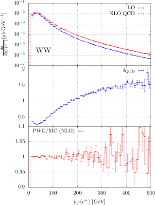
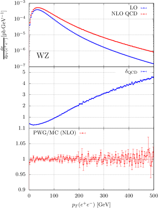
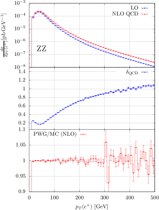
Figure 2: NLO QCD corrections to $pp\to e^{+}\nu_{e}\mu^{-}\overline{\nu}_{\mu}$ (top left), $pp\to\mu^{+}\nu_{\mu}e^{-}e^{+}$ (top right), and $pp\to\mu^{+}\mu^{-}e^{-}e^{+}$ (bottom) at the differential distribution level. Factorization and renormalization scales are set to the four-lepton invariant mass. Top panels: differential distributions at LO (blue) and NLO (red). Central panels: relative NLO corrections ($\delta=$NLO/LO-1). Lower panels: ratio of the NLO QCD predictions computed with POWHEG and MC. See main text for details.

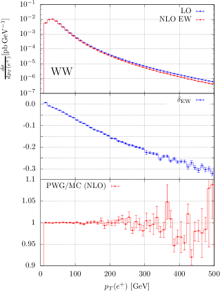
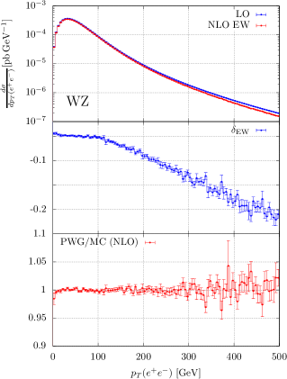
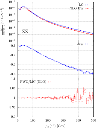
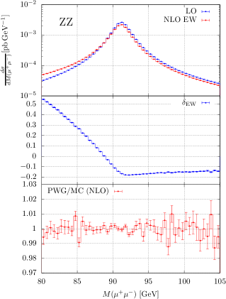
Figure 3: NLO EW corrections to $pp\to e^{+}\nu_{e}\mu^{-}\overline{\nu}_{\mu}$ (top left), $pp\to\mu^{+}\nu_{\mu}e^{-}e^{+}$ (top right), and $pp\to\mu^{+}\mu^{-}e^{-}e^{+}$ (bottom) at the differential distribution level. The factorization scale is set to $\mu=(M_{V}^{\rm\mathchoice{\displaystyle}{\scriptstyle}{\scriptscriptstyle}{\scriptscriptstyle}OS}+M_{V^{\prime}}^{\rm\mathchoice{\displaystyle}{\scriptstyle}{\scriptscriptstyle}{\scriptscriptstyle}OS})/2$ ($V,V^{\prime}=W,Z$). Top panels: differential distributions at LO (blue) and NLO (red). Central panels: relative NLO corrections ($\delta=$NLO/LO-1). Lower panels: ratio of the NLO EW predictions computed with POWHEG and MC. See main text for details.

In order to validate the implementation of the $\rm NLO_{\rm QCD}$ + $\rm NLO_{\rm EW}$ corrections to diboson-production processes in POWHEG-BOX-RES, we compare the predictions of our code with the ones of the Monte Carlo integrator used in Ref. [93] (MC in the following). Both codes use Recola2 for the calculation of the matrix elements, however, the integration and the subtraction of the IR singularities is performed in a completely independent way in the two programs. In particular, POWHEG uses the FKS subtraction (modified to take into account the presence of resonances), while in MC the Catani-Seymour procedure [105, 106] is used.

Tables 1-5 collect the results at the integrated cross-section level under the event selection of Eqs. (10) and (11) for the processes $pp\to e^{+}\nu_{e}\mu^{-}\overline{\nu}_{\mu}$, $pp\to\mu^{+}\nu_{\mu}e^{-}e^{+}$, and $pp\to\mu^{+}\mu^{-}e^{-}e^{+}$ (dubbed “WW”, “WZ”, and “ZZ” in the tables). Tables 1 and 2 show the results at LO for fixed and running scales, Tabs. 3 and 4 contain the results at $\rm NLO_{\rm QCD}$ for fixed and running scales, while the predictions at $\rm NLO_{\rm EW}$ accuracy (for fixed scales) are presented in Tab. 5. The $\rm NLO_{\rm QCD}$ corrections are positive, large and they are dominated by real QCD corrections: this is a consequence of the opening of gluon-induced channels ($qg\to VVq$) at $\rm NLO_{\rm QCD}$.

Since we are focused on the technical comparison of the two programs, we do not perform here scale-variation studies. The effect of scale variation can be read, for instance, from Ref. [93] and turns out to be large, given the size and the nature of the dominant contributions to the NLO QCD corrections.

The NLO EW corrections are negative and moderate at the integrated cross-section level. They are a combination of QED and purely weak effects.

In Tabs. 1-5, the numbers in parenthesis correspond to the statistical integration error on the last digit. As can be seen from Tabs. 1-5, the predictions of the two programs agree within the integration error.

The comparison at the differential distribution level is shown in Figs. 2 and 3 for the NLO QCD (running scales) and the NLO EW (fixed scales) predictions, respectively. For $WW$ and $ZZ$ production we consider the transverse momentum of the positron, $p_{\mathchoice{\displaystyle}{\scriptstyle}{\scriptscriptstyle}{\scriptscriptstyle}\rm T}(e^{+})$, while for $WZ$ production we take the transverse momentum of the $e^{+}e^{-}$ pair, $p_{\mathchoice{\displaystyle}{\scriptstyle}{\scriptscriptstyle}{\scriptscriptstyle}\rm T}(e^{+}e^{-})$, i.e. the reconstructed $Z$. For $ZZ$ production, we also present the results for the invariant mass of the $\mu^{+}\mu^{-}$ pair, $M(\mu^{+}\mu^{-})$. In Figs. 2 and 3, the upper panels show the differential distributions at LO (blue) and NLO (red) accuracy, the central panels show the relative NLO corrections ($\delta={\rm NLO}/{\rm LO}-1$), while, in the lower panels, we plot the ratio of the NLO predictions from POWHEG and MC. As largely discussed in the literature, the NLO QCD corrections to the transverse momentum observables are positive, large, and increase with $p_{\mathchoice{\displaystyle}{\scriptstyle}{\scriptscriptstyle}{\scriptscriptstyle}\rm T}$. On the contrary, the NLO QCD corrections to $M(\mu^{+}\mu^{-})$ are flat and correspond to a normalization factor. The NLO EW corrections to the transverse-momentum distributions are negative and show the typical Sudakov behaviour [107, 108, 109, 110, 111, 112, 113] at high $p_{\mathchoice{\displaystyle}{\scriptstyle}{\scriptscriptstyle}{\scriptscriptstyle}\rm T}$. The shape of the NLO EW corrections to $M(\mu^{+}\mu^{-})$ is dominated by QED effects, since the radiation of a final-state photon reduces the invariant mass of the lepton pair, shifting the events from the peak of the LO distribution to the region below the $Z$ resonance. As in the case of the cross-section level comparison, from the lower panels of Figs. 2 and 3 we conclude that POWHEG and MC agree within the statistical errors.

For the fixed-order part of the calculation, POWHEG computes the $\rm NLO_{\rm QCD}$ + $\rm NLO_{\rm EW}$ corrections additively. We checked that, when running our code with both QCD and EW corrections, $\delta_{\rm QCD+EW}$ from POWHEG is equal to the sum of $\delta_{\rm QCD}$ and $\delta_{\rm EW}$ computed with MC. We do not show here the plots, since the corresponding information can be read from the combination of Figs. 2 and 3.

5 Results at NLO+PS accuracy

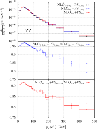
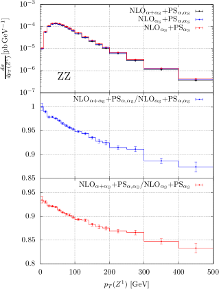
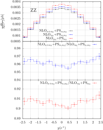
Figure 4: Comparison of the predictions at $\rm NLO_{\rm QCD}$ + $\rm NLO_{\rm EW}$ + $\rm PS_{{\rm QCD},{\rm QED}}$ (NLO${}_{\alpha+\alpha_{\rm S}}$+ PS${}_{\alpha,\alpha_{\rm S}}$), at $\rm NLO_{\rm QCD}$ + $\rm PS_{{\rm QCD},{\rm QED}}$ (NLO${}_{\alpha_{\rm S}}$+PS${}_{\alpha,\alpha_{\rm S}}$), and at $\rm NLO_{\rm QCD}$ + $\rm PS_{{\rm QCD}}$ (NLO${}_{\alpha_{\rm S}}$ + PS${}_{\alpha_{\rm S}}$) accuracy for the process $pp\to\mu^{+}\mu^{-}e^{-}e^{+}$. Upper panels: differential distributions as a function of the positron transverse momentum (top left), of the dimuon invariant mass (top right), of the transverse momentum of the hardest $Z$ (bottom left), and of the positron rapidity (bottom right). Central panels: ratio of the predictions at $\rm NLO_{\rm QCD}$ + $\rm NLO_{\rm EW}$ + $\rm PS_{{\rm QCD},{\rm QED}}$ and at $\rm NLO_{\rm QCD}$ + $\rm PS_{{\rm QCD},{\rm QED}}$. Lower panels: ratio of the results at $\rm NLO_{\rm QCD}$ + $\rm NLO_{\rm EW}$ + $\rm PS_{{\rm QCD},{\rm QED}}$ and at $\rm NLO_{\rm QCD}$ + $\rm PS_{{\rm QCD}}$. See main text for details.

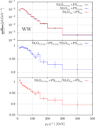
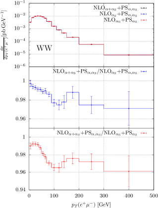
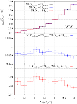
Figure 5: Comparison of the predictions at $\rm NLO_{\rm QCD}$ + $\rm NLO_{\rm EW}$ + $\rm PS_{{\rm QCD},{\rm QED}}$ (NLO${}_{\alpha+\alpha_{\rm S}}$+ PS${}_{\alpha,\alpha_{\rm S}}$), at $\rm NLO_{\rm QCD}$ + $\rm PS_{{\rm QCD},{\rm QED}}$ (NLO${}_{\alpha_{\rm S}}$+PS${}_{\alpha,\alpha_{\rm S}}$), and at $\rm NLO_{\rm QCD}$ + $\rm PS_{{\rm QCD}}$ (NLO${}_{\alpha_{\rm S}}$ + PS${}_{\alpha_{\rm S}}$) accuracy for the process $pp\to e^{+}\nu_{e}\mu^{-}\overline{\nu}_{\mu}$. Upper panels: differential distributions as a function of the positron transverse momentum (top left), of the transverse momentum (top right) and invariant mass (bottom left) of the positron–muon system, and of the azimuthal-angle separation between the positron and the muon (bottom right). Central panels: ratio of the predictions at $\rm NLO_{\rm QCD}$ + $\rm NLO_{\rm EW}$ + $\rm PS_{{\rm QCD},{\rm QED}}$ and at $\rm NLO_{\rm QCD}$ + $\rm PS_{{\rm QCD},{\rm QED}}$. Lower panels: ratio of the results at $\rm NLO_{\rm QCD}$ + $\rm NLO_{\rm EW}$ + $\rm PS_{{\rm QCD},{\rm QED}}$ and at $\rm NLO_{\rm QCD}$ + $\rm PS_{{\rm QCD}}$. See main text for details.

In this section, we present the results at NLO accuracy matched to PS. For brevity, we only show results for $ZZ$ and $WW$ production, but the code can be used to generate events and perform a similar study for $W^{\pm}Z$, as well. We consider three different levels of accuracy:

• $\rm NLO_{\rm QCD}$ + $\rm NLO_{\rm EW}$ + $\rm PS_{{\rm QCD},{\rm QED}}$: full NLO corrections matched to the full PS with QED and QCD radiation (NLO${}_{\alpha+\alpha_{\rm S}}$ + PS${}_{\alpha,\alpha_{\rm S}}$ in the plots);

• $\rm NLO_{\rm QCD}$ + $\rm PS_{{\rm QCD},{\rm QED}}$: strong corrections matched to the full PS (NLO${}_{\alpha_{\rm S}}$ + PS${}_{\alpha,\alpha_{\rm S}}$ in the plots);

• $\rm NLO_{\rm QCD}$ + $\rm PS_{{\rm QCD}}$: strong corrections matched to a PS without QED radiation (NLO${}_{\alpha_{\rm S}}$ + PS${}_{\alpha_{\rm S}}$ in the plots).

For the predictions at $\rm NLO_{\rm QCD}$ + $\rm NLO_{\rm EW}$ + $\rm PS_{{\rm QCD},{\rm QED}}$, according to the allrad scheme, our code generates up to three emissions, namely ISR QCD or QED radiation, and FSR QED radiation from the decay products of each one of the vector bosons. The kinematics of the hard partonic event generated by POWHEG, together with the values of the transverse momenta (with respect to their emitters) of the generated partonic and/or photonic radiation, is then saved in the Les Houches event file. The transverse momentum of the initial-state radiation, if present, is used by the parton shower algorithm as upper bound for the generation of QED/QCD radiation from the hard production process. The transverse momentum of the photons from the final-state leptons (i.e. from the resonances) is used by the parton shower program as upper bound for further QED radiation. The results presented in this paper have been showered by PYTHIA8. This code allows to veto emissions harder than the ones generated by POWHEG by using dedicated UserHooks. We have also verified that we obtain fully compatible results if we let the PS generate unconstrained emissions and we subsequently check if the transverse momentum of the radiations with respect to the emitting particles is smaller than the POWHEG hardest ones. If this is not the case, we attempt to shower the event again until all constraints are met and the event is accepted.

For the predictions at $\rm NLO_{\rm QCD}$ + $\rm PS_{{\rm QCD},{\rm QED}}$, the LH events contain at most one initial-state QCD radiation and the transverse momentum of the radiated parton sets the maximum hardness for the QCD PS, while the starting scale for the QED PS is the center of mass energy of the event for ISR, and the virtuality of the resonances for FSR. The predictions at $\rm NLO_{\rm QCD}$ matched to QCD PS are obtained from the same LH events used for the study at $\rm NLO_{\rm QCD}$ + $\rm PS_{{\rm QCD},{\rm QED}}$ accuracy, simply by turning off the QED radiation in PYTHIA.

In Figs. 4 and 5, the upper panels show the differential cross section as a function of the observable under consideration, the central panels contain the ratio of the results at $\rm NLO_{\rm QCD}$ + $\rm NLO_{\rm EW}$ + $\rm PS_{{\rm QCD},{\rm QED}}$ and the ones at $\rm NLO_{\rm QCD}$ + $\rm PS_{{\rm QCD},{\rm QED}}$, while, in the lower panels, we show the ratio of the predictions at $\rm NLO_{\rm QCD}$ + $\rm NLO_{\rm EW}$ + $\rm PS_{{\rm QCD},{\rm QED}}$ and the ones at $\rm NLO_{\rm QCD}$ + $\rm PS_{{\rm QCD}}$.

The calculation at $\rm NLO_{\rm QCD}$ + $\rm NLO_{\rm EW}$ accuracy matched to the full PS ($\rm PS_{{\rm QCD},{\rm QED}}$) includes the effect of the one-loop virtual weak corrections, the full QED corrections at $\mathcal{O}(\alpha)$, and part of the mixed factorized corrections at $\mathcal{O}(\alpha\alpha_{\rm S})$ (coming from the product of the NLO normalization encoded in the POWHEG $\bar{B}$ function and the Sudakov form factors in the POWHEG master formula for event generation [52]). Therefore the central panels of Figs. 4 and 5 show the effect of the weak NLO corrections, the difference between the exact QED corrections at $\mathcal{O}(\alpha)$ and their PS approximation, and the mixed corrections.

In the lower panels, the ratios are taken with respect to a result where only QCD corrections are included. Therefore, on top of the same effects as in the central panels, these panels also include the effect of all-order photonic corrections (without approximations at $\mathcal{O}(\alpha)$, and in PS approximation starting from $\mathcal{O}(\alpha^{2})$).

For the process $pp\to\mu^{+}\mu^{-}e^{-}e^{+}$ ($ZZ$ production, Fig. 4), besides the observables used in Sect. 4 for the validation at NLO ($p_{\mathchoice{\displaystyle}{\scriptstyle}{\scriptscriptstyle}{\scriptscriptstyle}\rm T}(e^{+})$ and $M(\mu^{+}\mu^{-})$), we consider the transverse momentum of the hardest reconstructed $Z$ boson, $p_{\mathchoice{\displaystyle}{\scriptstyle}{\scriptscriptstyle}{\scriptscriptstyle}\rm T}(Z^{1})$, and the positron rapidity, $y(e^{+})$. For the transverse-momentum distributions (left plots), the predictions at $\rm NLO_{\rm QCD}$ + $\rm NLO_{\rm EW}$ + $\rm PS_{{\rm QCD},{\rm QED}}$ are always lower than the ones at $\rm NLO_{\rm QCD}$ + $\rm PS_{{\rm QCD},{\rm QED}}$, or at $\rm NLO_{\rm QCD}$ + $\rm PS_{{\rm QCD}}$, in particular at high $p_{\mathchoice{\displaystyle}{\scriptstyle}{\scriptscriptstyle}{\scriptscriptstyle}\rm T}$, where the EW Sudakov corrections amount to approximately $-30$% with respect to the LO. The photonic corrections further reduce the predictions. The ratios for the positron rapidity distribution (bottom right plot) are essentially flat and, in the central panel, show an effect of about $-3/-4$% mainly coming from weak corrections that becomes approximately $-10$% in the lower panel, where the denominator does not include photonic corrections. The ratio of the predictions at $\rm NLO_{\rm QCD}$ + $\rm NLO_{\rm EW}$ + $\rm PS_{{\rm QCD},{\rm QED}}$ and the ones at $\rm NLO_{\rm QCD}$ + $\rm PS_{{\rm QCD},{\rm QED}}$ for the dimuon invariant-mass distribution (top right plot) is rather flat and shows that the effect of the EW corrections beyond QED PS amounts to about $-4$%. In the lower panel, there is a positive corrections below the $Z$ peak coming from multiple photon radiation (radiative return) very similar to the one observed at fixed order in Fig. 3.

The predictions at NLO+PS accuracy for the process $pp\to e^{+}\nu_{e}\mu^{-}\overline{\nu}_{\mu}$ ($WW$) are collected in Fig. 5 as a function of the following observables: transverse momentum of the positron, $p_{\mathchoice{\displaystyle}{\scriptstyle}{\scriptscriptstyle}{\scriptscriptstyle}\rm T}(e^{+})$, transverse momentum and invariant mass of the positron–muon system, $p_{\mathchoice{\displaystyle}{\scriptstyle}{\scriptscriptstyle}{\scriptscriptstyle}\rm T}(e^{+}\mu^{-})$ and $M(e^{+}\mu^{-})$, and azimuthal distance between the positron and the muon, $\Delta\phi(e^{+}\mu^{-})$. For all the observables under consideration, the inclusion of the NLO EW corrections lowers the predictions with respect to the calculation at $\rm NLO_{\rm QCD}$ + $\rm PS_{{\rm QCD},{\rm QED}}$ (central panels). This effect is more pronounced in the tails of the transverse-momentum and invariant-mass distributions, where the NLO EW corrections are negative and large because of the EW Sudakov logarithms. A comment is in order concerning the $p_{\mathchoice{\displaystyle}{\scriptstyle}{\scriptscriptstyle}{\scriptscriptstyle}\rm T}(e^{+}\mu^{-})$ distribution. In the high-$p_{\mathchoice{\displaystyle}{\scriptstyle}{\scriptscriptstyle}{\scriptscriptstyle}\rm T}$ tail, the errors are large and prevent a clean assessment of the size of the EW contributions. This is due to the fact that, in this region, the QCD corrections are positive, large, and increase very steeply starting from about 100 GeV in the absence of a jet veto. From the lower panels of Fig. 5, we conclude that the contribution of multiple photon radiation to the observables under consideration (with the event selection of Eq. (10)) is negative with the only exception of the first few bins of the $p_{\mathchoice{\displaystyle}{\scriptstyle}{\scriptscriptstyle}{\scriptscriptstyle}\rm T}(e^{+})$ and $M(e^{+}\mu^{-})$ distributions.

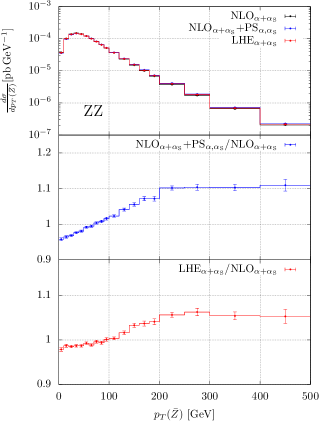
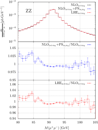
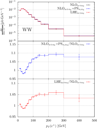
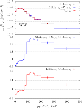
Figure 6: Comparison of the predictions at $\rm NLO_{\rm QCD}$ + $\rm NLO_{\rm EW}$ + $\rm PS_{{\rm QCD},{\rm QED}}$ (NLO${}_{\alpha+\alpha_{\rm S}}$+ PS${}_{\alpha,\alpha_{\rm S}}$), at LHE (LHE${}_{\alpha,\alpha_{\rm S}}$), and at fixed-order $\rm NLO_{\rm QCD}$ + $\rm NLO_{\rm EW}$ (NLO${}_{\alpha+\alpha_{\rm S}}$) accuracy for the processes $pp\to\mu^{+}\mu^{-}e^{-}e^{+}$ (upper plots) and $pp\to e^{+}\nu_{e}\mu^{-}\overline{\nu}_{\mu}$ (lower plots). Upper panels: differential distributions as a function of the transverse momentum of the same-flavour lepton pair, closer in virtuality to the nominal $Z$ mass (top left), of the dimuon invariant mass (top right), and of the transverse momentum of the positron (bottom left) and of the positron–muon system (bottom right). Central panels: ratio of the predictions at $\rm NLO_{\rm QCD}$ + $\rm NLO_{\rm EW}$ + $\rm PS_{{\rm QCD},{\rm QED}}$ and at fixed-order $\rm NLO_{\rm QCD}$ + $\rm NLO_{\rm EW}$ accuracy. Lower panels: ratio of the results at the LHE level and at fixed-order $\rm NLO_{\rm QCD}$ + $\rm NLO_{\rm EW}$ accuracy. See main text for details.

In order to further discuss effects beyond fixed order, in addition to those encountered so far, in Fig. 6 we show a few kinematic distributions at $\rm NLO_{\rm QCD}$ + $\rm NLO_{\rm EW}$ (NLO${}_{\alpha+\alpha_{\rm S}}$ in the plots, black lines), $\rm NLO_{\rm QCD}$ + $\rm NLO_{\rm EW}$ + $\rm PS_{{\rm QCD},{\rm QED}}$ (blue lines), and LHE (LHE${}_{\alpha+\alpha_{\rm S}}$ in the plots, red lines) accuracy. With “LHE” we denote the partonic results as predicted by POWHEG, after the generation of the hard radiation, but before a complete PS is performed. All the results in Fig. 6 include both QCD and EW corrections. Results for $ZZ$ production are shown in the upper row, where we consider the transverse momentum of the reconstructed $Z$ boson whose mass is closer to $M_{Z}$, and we indicate it with $p_{\mathchoice{\displaystyle}{\scriptstyle}{\scriptscriptstyle}{\scriptscriptstyle}\rm T}(\bar{Z})$ (left plot), and the invariant mass of the dimuon pair (right plot). In the lower row, we show results for $WW$ production, where we consider the transverse momentum of the positron (left plot) and the transverse momentum of the $e^{+}\mu^{-}$ pair (right plot).

We start our discussion from the dimuon pair invariant mass. We observe a relatively flat ratio between the fixed-order and the LHE result, slightly shifted below one, for values of $M(\mu^{+}\mu^{-})$ above the resonance peak, whereas below the peak the LHE prediction is larger than the NLO one. These trends are qualitatively similar to the $\rm NLO_{\rm EW}$/LO ratio $\delta_{\rm EW}$ shown in Fig. 3, and are mainly due to the radiative return, although here they are numerically much smaller, since the difference between the NLO and the LHE result comes essentially from the QED Sudakov form factor. Adding the PS does not change the picture, as the PS radiation starts at order $\alpha^{2}$ in the $\rm NLO_{\rm QCD}$ + $\rm NLO_{\rm EW}$ + $\rm PS_{{\rm QCD},{\rm QED}}$ calculation.

The $p_{\mathchoice{\displaystyle}{\scriptstyle}{\scriptscriptstyle}{\scriptscriptstyle}\rm T}(e^{+})$ and $p_{\mathchoice{\displaystyle}{\scriptstyle}{\scriptscriptstyle}{\scriptscriptstyle}\rm T}(\bar{Z})$ distributions are characterized by a similar trend in the hard region, where the ratio between the LHE and the NLO result is around 1.05 and is rather flat. The ratio of the showered and the NLO result is qualitatively similar, and is about 1.1. The difference between LHE and NLO+PS predictions is mainly due to QCD parton-shower radiation recoiling against the positron (or the $\bar{Z}$ system). At small transverse momenta, the ratios under consideration exhibit different patterns for the two observables. For the $p_{\mathchoice{\displaystyle}{\scriptstyle}{\scriptscriptstyle}{\scriptscriptstyle}\rm T}(\bar{Z})$ distribution, the LHE/NLO ratio is essentially equal to one, whereas the NLO+PS result receives a further (mild) suppression, due to multiple radiation. For the transverse momentum of the positron, $p_{\mathchoice{\displaystyle}{\scriptstyle}{\scriptscriptstyle}{\scriptscriptstyle}\rm T}(e^{+})$, the two ratio plots are qualitatively similar to the one shown in Fig. 2. Since QED radiative corrections play a smaller role (see Fig. 3), the shapes in Fig. 6 are mainly due to QCD corrections. The size of the effects displayed in Fig. 6 is significantly smaller than the one at fixed order, for reasons analogous to those discussed for the dimuon invariant mass, i.e. the ratio plots in Fig. 6 expose only higher-order corrections beyond the dominant ones.

Finally, we show the $p_{\mathchoice{\displaystyle}{\scriptstyle}{\scriptscriptstyle}{\scriptscriptstyle}\rm T}(e^{+}\mu^{-})$ distribution, that allows us to further elaborate on the origin of large QCD corrections for this process, and their impact on a matched NLO+PS simulation thereof. Below $p_{\mathchoice{\displaystyle}{\scriptstyle}{\scriptscriptstyle}{\scriptscriptstyle}\rm T}(e^{+}\mu^{-})\simeq$ 80 GeV, the LHE and the NLO+PS results are similar to each other, and they do not show very large differences from the fixed-order result, except for a moderate suppression when $p_{\mathchoice{\displaystyle}{\scriptstyle}{\scriptscriptstyle}{\scriptscriptstyle}\rm T}(e^{+}\mu^{-})\to 0$. Instead, at larger $p_{\mathchoice{\displaystyle}{\scriptstyle}{\scriptscriptstyle}{\scriptscriptstyle}\rm T}(e^{+}\mu^{-})$ values, the LHE result has a tail harder than at NLO, and this effect is even more marked at NLO+PS level. Similarly to what we have already alluded to when discussing Fig. 5, distortion effects for this distribution are due, by far, to the QCD corrections to diboson production, and they can be understood as follows: although the $p_{\mathchoice{\displaystyle}{\scriptstyle}{\scriptscriptstyle}{\scriptscriptstyle}\rm T}(e^{+}\mu^{-})$ distribution is inclusive with respect to the QCD emissions, it is kinematically correlated with the transverse momentum of the color-singlet system (denoted $p_{\mathchoice{\displaystyle}{\scriptstyle}{\scriptscriptstyle}{\scriptscriptstyle}\rm T}(WW)$ in the following). In particular, when $p_{\mathchoice{\displaystyle}{\scriptstyle}{\scriptscriptstyle}{\scriptscriptstyle}\rm T}(e^{+}\mu^{-})$ approaches small values, the kinematics is dominated by configurations where the color singlet is produced at small transverse momentum. Here all-order effects from soft ISR dominate, yielding a Sudakov suppression at small values of $p_{\mathchoice{\displaystyle}{\scriptstyle}{\scriptscriptstyle}{\scriptscriptstyle}\rm T}(WW)$, whose leftover is visible also in $p_{\mathchoice{\displaystyle}{\scriptstyle}{\scriptscriptstyle}{\scriptscriptstyle}\rm T}(e^{+}\mu^{-})$. For $p_{\mathchoice{\displaystyle}{\scriptstyle}{\scriptscriptstyle}{\scriptscriptstyle}\rm T}(e^{+}\mu^{-})$ larger than 80–100 GeV, the dominant kinematic configurations are those characterized by hard real QCD emissions. We have already discussed that the main effect comes from a vector boson recoiling against a hard jet, with the remaining vector boson being relatively soft. A jet-veto can substantially reduce this enhancement, keeping also the total $\rm NLO_{\rm QCD}$/LO $K$-factor closer to one. However, in Fig. 6 the ratios are taken with respect to the NLO result: at relatively large values, the $p_{\mathchoice{\displaystyle}{\scriptstyle}{\scriptscriptstyle}{\scriptscriptstyle}\rm T}$ distribution is dominated by QCD real radiation, and the ratio LHE/NLO shows a 20% enhancement in this region. This is a known POWHEG effect for processes with relatively large $K$-factors, first noticed in the context of inclusive Higgs boson production in gluon fusion [115]. It can be easily understood by considering the expression of the POWHEG differential cross section of Eq. (2) at large transverse momentum. In this kinematic region, the Sudakov form factor approaches 1, and the differential cross section behaves like

$$d\sigma\approx\frac{\bar{B}(\Phi_{B})}{B(\Phi_{B})}\left[R_{\rm\mathchoice{\displaystyle}{\scriptstyle}{\scriptscriptstyle}{\scriptscriptstyle}QCD}(\Phi_{B},\Phi_{\rm\mathchoice{\displaystyle}{\scriptstyle}{\scriptscriptstyle}{\scriptscriptstyle}rad})+R_{\rm\mathchoice{\displaystyle}{\scriptstyle}{\scriptscriptstyle}{\scriptscriptstyle}EW}(\Phi_{B},\Phi_{\rm\mathchoice{\displaystyle}{\scriptstyle}{\scriptscriptstyle}{\scriptscriptstyle}rad})\right]\,\mathrm{d}\Phi_{B}\,\mathrm{d}\Phi_{\rm\mathchoice{\displaystyle}{\scriptstyle}{\scriptscriptstyle}{\scriptscriptstyle}rad}\,,$$

displaying an enhancement of a factor $\bar{B}/B$ with respect to the real contribution. We stress that this effect is formally subleading, although, for the case at hand, amounts to about 20%. To reduce it, the use of hdamp was introduced in POWHEG. Essentially the real contribution is expressed as sum of two terms: one that approaches the full real contribution in the soft and collinear limit, and the other one that is finite in this limit. In Eqs. (2)–(4), only the singular term is used in the generation of the hardest radiation by POWHEG, while the other term, being finite and positive, is included in the remnant contribution. The scale hdamp is used to separate the two terms. In the present simulation, no such separation of the real contribution has been performed, so that in Eqs. (2)–(4) the full real matrix elements are used.

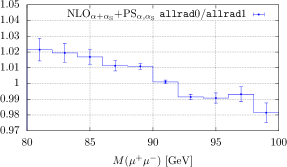
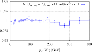
Figure 7: Ratio of the predictions at $\rm NLO_{\rm QCD}$ + $\rm NLO_{\rm EW}$ + $\rm PS_{{\rm QCD},{\rm QED}}$ accuracy computed with and without the allrad option (allrad1 and allrad0, respectively) for the invariant mass of the dimuon pair and the transverse momentum of the hardest $Z$ in $pp\to e^{+}e^{-}\mu^{+}\mu^{-}$. See main text for details.

The impact of the allrad option for the invariant mass of the dimuon pair and for the transverse momentum of the hardest $Z$ in $pp\to e^{+}e^{-}\mu^{+}\mu^{-}$ is displayed in Fig. 7. We find an effect of about 1-2% below the $Z$ resonance for the $M(\mu^{+}\mu^{-})$ distribution, where the QCD corrections are a flat normalization factor, while the QED corrections lead to large shape distortions. This is due to the fact that, without the allrad option, the upper scale for the generation of radiation used by the PS program is set by the transverse momentum of the hardest radiation generated by POWHEG, that, in most cases, is ISR QCD. This upper scale is then used, by the PS, for both the ISR (QCD and QED) and the FSR QED radiation. As a result, the FSR QED radiation from PS can be harder than the one that would have been generated by POWHEG and the predictions obtained without the allrad option show larger radiative return effects compared to the ones computed with the allrad option. At variance with the invariant-mass distribution, for the $p_{\mathchoice{\displaystyle}{\scriptstyle}{\scriptscriptstyle}{\scriptscriptstyle}\rm T}$ of the hardest Z, where the QCD corrections are much larger than the EW ones, the effect of the allrad option is not visible with the statistics used in this paper. The results shown in Fig. 7 agree with the ones obtained in Ref. [72] for Drell-Yan production.

Before drawing our conclusions, we would like to comment further on the possible sources of theoretical uncertainties that affect our calculation. We stress that, as far as the perturbative uncertainties are concerned, all these effects are of higher orders, beyond the $\rm NLO_{\rm QCD}$ + $\rm NLO_{\rm EW}$ + PS accuracy of the presented results. The main source of theoretical uncertainties are the perturbative ones related to the choice of the renormalization and factorization scales, and the non-perturbative ones coming from the choice of the parton distribution functions. It is possible to estimate these uncertainties through scale variations and using several PDF sets. The impact of scale variation at $\rm NLO_{\rm QCD}$ for the processes under consideration can be found, for instance, in Ref. [93]. The theoretical uncertainties associated with the missing higher-order EW corrections are expected to have a minor impact and can be estimated by changing the EW input parameters/renormalization schemes using the flag scheme in the input card to select the $(\alpha_{0},M_{W},M_{Z})$, $(\alpha(M_{Z}),M_{W},M_{Z})$, or $(G_{\mu},M_{W},M_{Z})$ schemes.

Photon-induced processes contribute at the same perturbative order of the $\rm NLO_{\rm EW}$ corrections (for $WW$ and $ZZ$ they also contribute at LO): at present, these processes are not included in our calculation and their contribution is a theoretical uncertainty for the results presented in this paper. The study of their effect in a NLO+PS simulation will be the subject of future investigations

As stated in Sect. 1, the POWHEG algorithm applied to the case of $\rm NLO_{\rm QCD}$+$\rm NLO_{\rm EW}$ corrections gives as a by-product mixed corrections of the form $\mathcal{O}(\alpha_{\mathchoice{\displaystyle}{\scriptstyle}{\scriptscriptstyle}{\scriptscriptstyle}\rm S}^{n}\alpha^{m})$. This is an approximation of the factorizable mixed QCD-EW corrections that is only reliable in the collinear limit. For diboson production processes, this approximation is expected to work for distributions like the vector-bosons virtualities in the regions close to the resonances (similarly to what happens for Drell-Yan [72]), while it is expected to fail in the high-$p_{\mathchoice{\displaystyle}{\scriptstyle}{\scriptscriptstyle}{\scriptscriptstyle}\rm T}$ regions, where the QCD corrections are very large and dominated by hard QCD radiation [65]. Although the reliability of the mixed effect provided by POWHEG can only be assessed through comparison with full calculations at $\mathcal{O}(\alpha\alpha_{S})$, when such calculations will be available, an estimate of the related uncertainties can be obtained by comparing the results at $\rm NLO_{\rm QCD}$ + $\rm NLO_{\rm EW}$ + PS accuracy for diboson and diboson + jet production (possibly merged with the results for $pp\to VV^{\prime}$).

Another class of uncertainties is related to the matching procedure, such as the scale choice for the parameter hdamp, or the use of the allrad option. In addition, different PS algorithms use different ordering variables, and such choices have a non negligible impact on the kinematic distributions. The present release of the code presented in this paper only includes an interface to PYTHIA8.2, however, in order to study this class of uncertainties, dedicated interfaces to other shower Monte Carlo programs (like, for instance, PHOTOS [116, 117, 118] for the QED FSR) could be developed.

A comprehensive study of the theoretical uncertainties described above goes beyond the scope of this work, however, the event generator presented in this paper could be used in particular by the experimental collaborations to asses the different classes of theoretical uncertainties that affect the calculation at hand.

6 Conclusions

We computed the NLO QCD + NLO EW corrections to diboson production at hadron colliders matched to a complete parton shower, where QCD and QED radiation is simulated. For diboson production this is the first calculation where the NLO EW corrections have been consistently matched to QED PS. As the considered processes involve the production and the decay of unstable particles, whose decay products can radiate photons, the calculation is based on the POWHEG-BOX-RES framework. The corresponding code is public and all the information for downloading it can be found in the POWHEG-BOX web page.

Though we did not perform an extensive phenomenological study that might be the subject of a future publication, we showed the potential of our code, and we pointed out that EW effects, consistently matched to QED parton shower, are relevant for several observables of interest.

The code relies on the Recola2 library for the calculation of the matrix elements for four leptons and four leptons plus photon/parton production. In particular, we developed a fully general interface between POWHEG-BOX and Recola2 that could be used for other processes. We performed our calculation in the Standard Model. However, given the possibility of Recola2 to compute tree-level and one-loop matrix elements in general extensions of the SM, in the future the code could be easily generalized to compute the NLO QCD + NLO EW corrections to diboson production matched to QCD and QED parton shower in the context of models beyond the SM, provided that the one-loop corrections are available in Recola2, and that the considered model does not alter the structure of QED and QCD interactions in a non-trivial way. If this were the case, the subtraction of infrared singularities and the Sudakov form factors in the POWHEG-BOX-RES should also be generalized.

As a final remark, the effect of NLO QCD corrections to diboson production is very large and it is dominated by real parton radiation, especially in the regions where one of the two vector bosons is soft with respect to the jet. It is thus important to include QCD corrections beyond NLO accuracy, for instance using a consistent merging of the predictions for $VV^{\prime}$ and $VV^{\prime}$+ jet production ($V,V^{\prime}=W,Z$) based on the MiNLO [63] or MiNNLO_PS [119] procedures (at NLO and NNLO accuracy, respectively). The code presented in this paper can be taken as the starting point for the inclusion of the EW effects matched to QED PS in the treatment of diboson (+ jet) production in the MiNLO or MiNNLO_PS framework.

Acknowledgements

The work of M.C. has been supported by the “Investissements d’avenir, Labex ENIGMASS”.

References

- [1] K. Hagiwara, R. Peccei, D. Zeppenfeld, K. Hikasa, Nucl. Phys. B 282, 253 (1987). DOI 10.1016/0550-3213(87)90685-7
- [2] C. Frye, M. Freytsis, J. Scholtz, M.J. Strassler, JHEP 03, 171 (2016). DOI 10.1007/JHEP03(2016)171
- [3] A. Butter, O.J.P. Éboli, J. Gonzalez-Fraile, M. Gonzalez-Garcia, T. Plehn, M. Rauch, JHEP 07, 152 (2016). DOI 10.1007/JHEP07(2016)152
- [4] Z. Zhang, Phys. Rev. Lett. 118(1), 011803 (2017). DOI 10.1103/PhysRevLett.118.011803
- [5] D.R. Green, P. Meade, M.A. Pleier, Rev. Mod. Phys. 89(3), 035008 (2017). DOI 10.1103/RevModPhys.89.035008
- [6] J. Baglio, S. Dawson, I.M. Lewis, Phys. Rev. D 96(7), 073003 (2017). DOI 10.1103/PhysRevD.96.073003
- [7] A. Falkowski, M. Gonzalez-Alonso, A. Greljo, D. Marzocca, M. Son, JHEP 02, 115 (2017). DOI 10.1007/JHEP02(2017)115
- [8] G. Panico, F. Riva, A. Wulzer, Phys. Lett. B 776, 473 (2018). DOI 10.1016/j.physletb.2017.11.068
- [9] R. Franceschini, G. Panico, A. Pomarol, F. Riva, A. Wulzer, JHEP 02, 111 (2018). DOI 10.1007/JHEP02(2018)111
- [10] J. Baglio, S. Dawson, I.M. Lewis, Phys. Rev. D 99(3), 035029 (2019). DOI 10.1103/PhysRevD.99.035029
- [11] J. Baglio, S. Dawson, S. Homiller, Phys. Rev. D 100(11), 113010 (2019). DOI 10.1103/PhysRevD.100.113010
- [12] D. Liu, L.T. Wang, Phys. Rev. D 99(5), 055001 (2019). DOI 10.1103/PhysRevD.99.055001
- [13] A. Azatov, D. Barducci, E. Venturini, JHEP 04, 075 (2019). DOI 10.1007/JHEP04(2019)075
- [14] J. Ohnemus, Phys. Rev. D 50, 1931 (1994). DOI 10.1103/PhysRevD.50.1931
- [15] L.J. Dixon, Z. Kunszt, A. Signer, Phys. Rev. D 60, 114037 (1999). DOI 10.1103/PhysRevD.60.114037
- [16] J.M. Campbell, R. Ellis, Phys. Rev. D 60, 113006 (1999). DOI 10.1103/PhysRevD.60.113006
- [17] J.M. Campbell, R. Ellis, C. Williams, JHEP 07, 018 (2011). DOI 10.1007/JHEP07(2011)018
- [18] M. Grazzini, S. Kallweit, D. Rathlev, Phys. Lett. B 750, 407 (2015). DOI 10.1016/j.physletb.2015.09.055
- [19] M. Grazzini, S. Kallweit, D. Rathlev, M. Wiesemann, Phys. Lett. B 761, 179 (2016). DOI 10.1016/j.physletb.2016.08.017
- [20] M. Grazzini, S. Kallweit, S. Pozzorini, D. Rathlev, M. Wiesemann, JHEP 08, 140 (2016). DOI 10.1007/JHEP08(2016)140
- [21] M. Grazzini, S. Kallweit, D. Rathlev, M. Wiesemann, JHEP 05, 139 (2017). DOI 10.1007/JHEP05(2017)139
- [22] G. Heinrich, S. Jahn, S. Jones, M. Kerner, J. Pires, JHEP 03, 142 (2018). DOI 10.1007/JHEP03(2018)142
- [23] S. Kallweit, M. Wiesemann, Phys. Lett. B 786, 382 (2018). DOI 10.1016/j.physletb.2018.10.016
- [24] M. Grazzini, S. Kallweit, M. Wiesemann, Eur. Phys. J. C 78(7), 537 (2018). DOI 10.1140/epjc/s10052-018-5771-7
- [25] T. Binoth, M. Ciccolini, N. Kauer, M. Kramer, JHEP 03, 065 (2005). DOI 10.1088/1126-6708/2005/03/065
- [26] C. Zecher, T. Matsuura, J. van der Bij, Z. Phys. C 64, 219 (1994). DOI 10.1007/BF01557393
- [27] T. Binoth, M. Ciccolini, N. Kauer, M. Kramer, JHEP 12, 046 (2006). DOI 10.1088/1126-6708/2006/12/046
- [28] F. Caola, K. Melnikov, R. Röntsch, L. Tancredi, Phys. Lett. B 754, 275 (2016). DOI 10.1016/j.physletb.2016.01.046
- [29] F. Caola, K. Melnikov, R. Röntsch, L. Tancredi, Phys. Rev. D 92(9), 094028 (2015). DOI 10.1103/PhysRevD.92.094028
- [30] M. Grazzini, S. Kallweit, M. Wiesemann, J.Y. Yook, JHEP 03, 070 (2019). DOI 10.1007/JHEP03(2019)070
- [31] M. Grazzini, S. Kallweit, M. Wiesemann, J.Y. Yook, Phys. Lett. B 804, 135399 (2020). DOI 10.1016/j.physletb.2020.135399
- [32] B. Biedermann, M. Billoni, A. Denner, S. Dittmaier, L. Hofer, B. Jäger, L. Salfelder, JHEP 06, 065 (2016). DOI 10.1007/JHEP06(2016)065
- [33] B. Biedermann, A. Denner, S. Dittmaier, L. Hofer, B. Jäger, Phys. Rev. Lett. 116(16), 161803 (2016). DOI 10.1103/PhysRevLett.116.161803
- [34] B. Biedermann, A. Denner, S. Dittmaier, L. Hofer, B. Jager, JHEP 01, 033 (2017). DOI 10.1007/JHEP01(2017)033
- [35] B. Biedermann, A. Denner, L. Hofer, JHEP 10, 043 (2017). DOI 10.1007/JHEP10(2017)043
- [36] S. Kallweit, J. Lindert, S. Pozzorini, M. Schönherr, JHEP 11, 120 (2017). DOI 10.1007/JHEP11(2017)120
- [37] A. Bierweiler, T. Kasprzik, J.H. Kühn, S. Uccirati, JHEP 11, 093 (2012). DOI 10.1007/JHEP11(2012)093
- [38] A. Bierweiler, T. Kasprzik, J.H. Kühn, JHEP 12, 071 (2013). DOI 10.1007/JHEP12(2013)071
- [39] J. Baglio, L.D. Ninh, M.M. Weber, Phys. Rev. D 88, 113005 (2013). DOI 10.1103/PhysRevD.94.099902. [Erratum: Phys.Rev.D 94, 099902 (2016)]
- [40] J. Kuhn, F. Metzler, A. Penin, S. Uccirati, JHEP 06, 143 (2011). DOI 10.1007/JHEP06(2011)143
- [41] P. Meade, H. Ramani, M. Zeng, Phys. Rev. D90(11), 114006 (2014). DOI 10.1103/PhysRevD.90.114006
- [42] M. Grazzini, S. Kallweit, D. Rathlev, M. Wiesemann, JHEP 08, 154 (2015). DOI 10.1007/JHEP08(2015)154
- [43] T. Becher, M. Hager, Eur. Phys. J. C 79(8), 665 (2019). DOI 10.1140/epjc/s10052-019-7136-2
- [44] T. Becher, R. Frederix, M. Neubert, L. Rothen, Eur. Phys. J. C75(4), 154 (2015). DOI 10.1140/epjc/s10052-015-3368-y
- [45] S. Dawson, P. Jaiswal, Y. Li, H. Ramani, M. Zeng, Phys. Rev. D94(11), 114014 (2016). DOI 10.1103/PhysRevD.94.114014
- [46] L. Arpino, A. Banfi, S. Jäger, N. Kauer, JHEP 08, 076 (2019). DOI 10.1007/JHEP08(2019)076
- [47] S. Kallweit, E. Re, L. Rottoli, M. Wiesemann, arXiv:2004.07720
- [48] S. Frixione, B.R. Webber, JHEP 06, 029 (2002). DOI 10.1088/1126-6708/2002/06/029
- [49] P. Nason, JHEP 11, 040 (2004). DOI 10.1088/1126-6708/2004/11/040
- [50] S. Frixione, P. Nason, C. Oleari, JHEP 11, 070 (2007). DOI 10.1088/1126-6708/2007/11/070
- [51] J. Alwall, R. Frederix, S. Frixione, V. Hirschi, F. Maltoni, O. Mattelaer, H.S. Shao, T. Stelzer, P. Torrielli, M. Zaro, JHEP 07, 079 (2014). DOI 10.1007/JHEP07(2014)079
- [52] S. Alioli, P. Nason, C. Oleari, E. Re, JHEP 06, 043 (2010). DOI 10.1007/JHEP06(2010)043
- [53] S. Hoeche, F. Krauss, M. Schonherr, F. Siegert, JHEP 09, 049 (2012). DOI 10.1007/JHEP09(2012)049
- [54] E. Bothmann, et al., SciPost Phys. 7(3), 034 (2019). DOI 10.21468/SciPostPhys.7.3.034
- [55] J. Bellm, et al., Eur. Phys. J. C 76(4), 196 (2016). DOI 10.1140/epjc/s10052-016-4018-8
- [56] S. Platzer, S. Gieseke, Eur. Phys. J. C 72, 2187 (2012). DOI 10.1140/epjc/s10052-012-2187-7
- [57] T. Melia, P. Nason, R. Rontsch, G. Zanderighi, JHEP 11, 078 (2011). DOI 10.1007/JHEP11(2011)078
- [58] R. Frederix, S. Frixione, V. Hirschi, F. Maltoni, R. Pittau, P. Torrielli, JHEP 02, 099 (2012). DOI 10.1007/JHEP02(2012)099
- [59] F. Cascioli, S. Höche, F. Krauss, P. Maierhöfer, S. Pozzorini, F. Siegert, JHEP 01, 046 (2014). DOI 10.1007/JHEP01(2014)046
- [60] P. Nason, G. Zanderighi, Eur. Phys. J. C 74(1), 2702 (2014). DOI 10.1140/epjc/s10052-013-2702-5
- [61] S. Alioli, F. Caola, G. Luisoni, R. Röntsch, Phys. Rev. D 95(3), 034042 (2017). DOI 10.1103/PhysRevD.95.034042
- [62] K. Hamilton, T. Melia, P.F. Monni, E. Re, G. Zanderighi, JHEP 09, 057 (2016). DOI 10.1007/JHEP09(2016)057
- [63] K. Hamilton, P. Nason, C. Oleari, G. Zanderighi, JHEP 05, 082 (2013). DOI 10.1007/JHEP05(2013)082
- [64] E. Re, M. Wiesemann, G. Zanderighi, JHEP 12, 121 (2018). DOI 10.1007/JHEP12(2018)121
- [65] M. Grazzini, S. Kallweit, J.M. Lindert, S. Pozzorini, M. Wiesemann, JHEP 02, 087 (2020). DOI 10.1007/JHEP02(2020)087
- [66] S. Kallweit, J.M. Lindert, P. Maierhofer, S. Pozzorini, M. Schönherr, JHEP 04, 021 (2016). DOI 10.1007/JHEP04(2016)021
- [67] S. Bräuer, A. Denner, M. Pellen, M. Schönherr, S. Schumann, arXiv:2005.12128
- [68] T. Ježo, P. Nason, JHEP 12, 065 (2015). DOI 10.1007/JHEP12(2015)065
- [69] T. Ježo, J.M. Lindert, P. Nason, C. Oleari, S. Pozzorini, Eur. Phys. J. C 76(12), 691 (2016). DOI 10.1140/epjc/s10052-016-4538-2
- [70] F. Granata, J.M. Lindert, C. Oleari, S. Pozzorini, JHEP 09, 012 (2017). DOI 10.1007/JHEP09(2017)012
- [71] M. Chiesa, A. Denner, J.N. Lang, M. Pellen, Eur. Phys. J. C 79(9), 788 (2019). DOI 10.1140/epjc/s10052-019-7290-6
- [72] C.M. Carloni Calame, M. Chiesa, H. Martinez, G. Montagna, O. Nicrosini, F. Piccinini, A. Vicini, Phys. Rev. D 96(9), 093005 (2017). DOI 10.1103/PhysRevD.96.093005
- [73] L. Barze, G. Montagna, P. Nason, O. Nicrosini, F. Piccinini, JHEP 04, 037 (2012). DOI 10.1007/JHEP04(2012)037
- [74] L. Barze, G. Montagna, P. Nason, O. Nicrosini, F. Piccinini, A. Vicini, Eur. Phys. J. C 73(6), 2474 (2013). DOI 10.1140/epjc/s10052-013-2474-y
- [75] M. Chiesa, F. Piccinini, A. Vicini, Phys. Rev. D 100(7), 071302 (2019). DOI 10.1103/PhysRevD.100.071302
- [76] C. Bernaciak, D. Wackeroth, Phys. Rev. D 85, 093003 (2012). DOI 10.1103/PhysRevD.85.093003
- [77] A. Mück, L. Oymanns, JHEP 05, 090 (2017). DOI 10.1007/JHEP05(2017)090
- [78] S. Frixione, Z. Kunszt, A. Signer, Nucl. Phys. B 467, 399 (1996). DOI 10.1016/0550-3213(96)00110-1
- [79] J.M. Campbell, R.K. Ellis, P. Nason, E. Re, JHEP 04, 114 (2015). DOI 10.1007/JHEP04(2015)114
- [80] S. Actis, A. Denner, L. Hofer, A. Scharf, S. Uccirati, JHEP 04, 037 (2013). DOI 10.1007/JHEP04(2013)037
- [81] S. Actis, A. Denner, L. Hofer, J.N. Lang, A. Scharf, S. Uccirati, Comput. Phys. Commun. 214, 140 (2017). DOI 10.1016/j.cpc.2017.01.004
- [82] A. Denner, J.N. Lang, S. Uccirati, JHEP 07, 087 (2017). DOI 10.1007/JHEP07(2017)087
- [83] A. Denner, J.N. Lang, S. Uccirati, Comput. Phys. Commun. 224, 346 (2018). DOI 10.1016/j.cpc.2017.11.013
- [84] A. Denner, S. Dittmaier, Nucl. Phys. B 844, 199 (2011). DOI 10.1016/j.nuclphysb.2010.11.002
- [85] A. Denner, S. Dittmaier, Nucl. Phys. B 658, 175 (2003). DOI 10.1016/S0550-3213(03)00184-6
- [86] A. Denner, S. Dittmaier, Nucl. Phys. B 734, 62 (2006). DOI 10.1016/j.nuclphysb.2005.11.007
- [87] A. Denner, S. Dittmaier, L. Hofer, Comput. Phys. Commun. 212, 220 (2017). DOI 10.1016/j.cpc.2016.10.013
- [88] B. Biedermann, A. Denner, M. Pellen, JHEP 10, 124 (2017). DOI 10.1007/JHEP10(2017)124
- [89] A. Denner, S. Dittmaier, M. Roth, D. Wackeroth, Nucl. Phys. B 560, 33 (1999). DOI 10.1016/S0550-3213(99)00437-X
- [90] A. Denner, S. Dittmaier, M. Roth, L. Wieders, Nucl. Phys. B 724, 247 (2005). DOI 10.1016/j.nuclphysb.2011.09.001. [Erratum: Nucl.Phys.B 854, 504–507 (2012)]
- [91] A. Denner, S. Dittmaier, Nucl. Phys. B Proc. Suppl. 160, 22 (2006). DOI 10.1016/j.nuclphysbps.2006.09.025
- [92] S. Alioli, P. Nason, C. Oleari, E. Re, JHEP 01, 095 (2011). DOI 10.1007/JHEP01(2011)095
- [93] M. Chiesa, A. Denner, J.N. Lang, Eur. Phys. J. C 78(6), 467 (2018). DOI 10.1140/epjc/s10052-018-5949-z
- [94] R.D. Ball, et al., Nucl. Phys. B 867, 244 (2013). DOI 10.1016/j.nuclphysb.2012.10.003
- [95] R.D. Ball, V. Bertone, S. Carrazza, L. Del Debbio, S. Forte, A. Guffanti, N.P. Hartland, J. Rojo, Nucl. Phys. B 877, 290 (2013). DOI 10.1016/j.nuclphysb.2013.10.010
- [96] R.D. Ball, et al., JHEP 04, 040 (2015). DOI 10.1007/JHEP04(2015)040
- [97] R.D. Ball, et al., Eur. Phys. J. C 77(10), 663 (2017). DOI 10.1140/epjc/s10052-017-5199-5
- [98] L. Harland-Lang, A. Martin, P. Motylinski, R. Thorne, Eur. Phys. J. C 75(5), 204 (2015). DOI 10.1140/epjc/s10052-015-3397-6
- [99] T.J. Hou, et al., (2019). arXiv:1912.10053
- [100] A. Buckley, J. Ferrando, S. Lloyd, K. Nordström, B. Page, M. Rüfenacht, M. Schönherr, G. Watt, Eur. Phys. J. C 75, 132 (2015). DOI 10.1140/epjc/s10052-015-3318-8
- [101] T. Sjostrand, S. Mrenna, P.Z. Skands, JHEP 05, 026 (2006). DOI 10.1088/1126-6708/2006/05/026
- [102] T. Sjöstrand, S. Ask, J.R. Christiansen, R. Corke, N. Desai, P. Ilten, S. Mrenna, S. Prestel, C.O. Rasmussen, P.Z. Skands, Comput. Phys. Commun. 191, 159 (2015). DOI 10.1016/j.cpc.2015.01.024
- [103] M. Cacciari, G.P. Salam, Phys. Lett. B 641, 57 (2006). DOI 10.1016/j.physletb.2006.08.037
- [104] M. Cacciari, G.P. Salam, G. Soyez, Eur. Phys. J. C 72, 1896 (2012). DOI 10.1140/epjc/s10052-012-1896-2
- [105] S. Catani, M. Seymour, Nucl. Phys. B 485, 291 (1997). DOI 10.1016/S0550-3213(96)00589-5. [Erratum: Nucl.Phys.B 510, 503–504 (1998)]
- [106] S. Dittmaier, Nucl. Phys. B 565, 69 (2000). DOI 10.1016/S0550-3213(99)00563-5
- [107] W. Beenakker, A. Denner, S. Dittmaier, R. Mertig, T. Sack, Nucl. Phys. B 410, 245 (1993). DOI 10.1016/0550-3213(93)90434-Q
- [108] M. Beccaria, G. Montagna, F. Piccinini, F. Renard, C. Verzegnassi, Phys. Rev. D 58, 093014 (1998). DOI 10.1103/PhysRevD.58.093014
- [109] P. Ciafaloni, D. Comelli, Phys. Lett. B 446, 278 (1999). DOI 10.1016/S0370-2693(98)01541-X
- [110] J.H. Kuhn, A. Penin, (1999). hep-ph/9906545
- [111] M. Ciafaloni, P. Ciafaloni, D. Comelli, Phys. Rev. Lett. 84, 4810 (2000). DOI 10.1103/PhysRevLett.84.4810
- [112] A. Denner, S. Pozzorini, Eur. Phys. J. C 18, 461 (2001). DOI 10.1007/s100520100551
- [113] A. Denner, S. Pozzorini, Eur. Phys. J. C 21, 63 (2001). DOI 10.1007/s100520100721
- [114] M. Rubin, G.P. Salam, S. Sapeta, JHEP 09, 084 (2010). DOI 10.1007/JHEP09(2010)084
- [115] S. Alioli, P. Nason, C. Oleari, E. Re, JHEP 04, 002 (2009). DOI 10.1088/1126-6708/2009/04/002
- [116] E. Barberio, B. van Eijk, Z. Was, Comput. Phys. Commun. 66, 115 (1991). DOI 10.1016/0010-4655(91)90012-A
- [117] E. Barberio, Z. Was, Comput. Phys. Commun. 79, 291 (1994). DOI 10.1016/0010-4655(94)90074-4
- [118] P. Golonka, Z. Was, Eur. Phys. J. C 45, 97 (2006). DOI 10.1140/epjc/s2005-02396-4
- [119] P.F. Monni, P. Nason, E. Re, M. Wiesemann, G. Zanderighi, JHEP 05, 143 (2020). DOI 10.1007/JHEP05(2020)143