The Fornax Deep Survey with VST. IX

Abstract

Context. A possible pathway for understanding the events and the mechanisms involved in galaxy formation and evolution is an in-depth comprehension of the galactic and inter-galactic fossil sub-structures with long dynamical times-scales: stars in the field and in stellar clusters.

Aims. This paper continues the series of the Fornax Deep Survey (FDS). Following the previous studies dedicated to extended Fornax cluster members, in this paper we present the catalogs of compact stellar systems in the Fornax cluster as well as extended background sources and point-like sources.

Methods. We derive $ugri$ photometry of $\sim 1.7$ million sources over the $\sim 21$ square degree area of FDS centered on the bright central galaxy NGC 1399. For a wider area, of $\sim 27$ square degrees extending in the direction of NGC 1316, we provide $gri$ photometry for $\sim 3.1$ million sources. To improve the morphological characterization of sources we generate multi-band image stacks by coadding the best seeing $gri$-band single exposures with a cut at FWHM$\leq 0\aas@@fstack{\prime\prime}9$. We use the multi-band stacks as master detection frames, with a FWHM improved by $\sim 15\%$ and a FWHM variability from field to field reduced by a factor of $\sim 2.5$ compared to the pass-band with best FWHM, namely the $r$-band. The identification of compact sources, in particular of globular clusters (GC), is obtained from a combination of photometric (e.g. colors, magnitudes) and morphometric (e.g. concentration index, elongation, effective radius) selection criteria, by also taking as reference the properties of sources with well-defined classification from spectroscopic or high-resolution imaging data.

Results. Using the FDS catalogs, we present a preliminary analysis of globular cluster (GC) distributions in the Fornax area. The study confirms and extends further previous results which were limited to a smaller survey area. We observe the inter-galactic population of GCs, a population of mainly blue GCs centered on NGC 1399, extends over $\sim 0.9$ Mpc, with an ellipticity $\epsilon\sim 0.65$ and a small tilt in the direction of NGC 1336. Several sub-structures extend over $\sim 0.5\leavevmode\nobreak\ Mpc$ along various directions. Two of these structures do not cross any bright galaxy; one of them appears to be connected to NGC 1404, a bright galaxy close to the cluster core and particularly poor of GCs. Using the $gri$ catalogs we analyze the GC distribution over the extended FDS area, and do not find any obvious GC sub-structure bridging the two brightest cluster galaxies, NGC 1316 and NGC 1399. Although NGC 1316 is more than twice brighter of NGC 1399 in optical bands, using $gri$ data, we estimate a factor of $\sim 3-4$ richer GC population around NGC 1399 compared to NGC 1316, out to galactocentric distances of $\sim 40\arcmin$ or $\sim 230$ kpc.

Conclusions. The $ugri$ and $gri$ catalogs we present are made public via the FDS project web pages, and through the virtual observatory. Further studies, based on the catalogs, are in progress.

1 Introduction

The study of local complexes of galaxies –galaxy clusters and groups– is crucial for our understanding of the history of formation and evolution of the Universe through its building blocks. Local galaxy systems mark the endpoint of the evolution of galaxies after billion years of more or less intense interaction with their companions (e.g. Mo et al., 2010).

A detailed study of the two extreme structures in terms of stellar density gives precious information on the history of formation and interactions of a galaxy: faint extended stellar features in the outskirts of galaxies, characterized by low star density and very long dynamical mixing time-scales (Johnston et al., 2008), and compact stellar systems, which are intrinsically bright, have typically old ages and have orbits that can trace recent and ancient accretion events (Brodie & Strader, 2006). The stratification of dense star clusters and low surface brightness features can probe a galaxy environment on different time scales, from the earliest epoch of formation to the most recent merging events (e.g. West et al., 2004; Bournaud, 2011).

In the last decade, also thanks to the advent of efficient large-format imaging cameras, many observational programs have carried out intensive surveys dedicated to cover large fractions of nearby galaxy systems, superseding in terms of both limiting magnitude and spatial resolution any previous optical/near-IR study (e.g. Ferrarese et al., 2012; Iodice et al., 2016), and providing a rich variety of data ideal for investigating compact stellar systems and faint stellar structures in different galaxy environments (de Jong et al., 2013; Muñoz et al., 2014; Durrell et al., 2014; Iodice et al., 2019; Venhola et al., 2019; Wittmann et al., 2019)

In this framework, the Fornax Deep Survey, FDS, has surveyed the Fornax galaxy cluster centered on NGC 1399 out to one virial radius, and further extended observations in the direction of the Fornax A sub-cluster in the South-West with its brightest member, NGC 1316, with a list of scientific topics: diffuse light and intracluster medium (Iodice et al., 2016), galaxy scaling relations (Iodice et al., 2019; Venhola et al., 2017, 2019; Raj et al., 2019), extragalactic star clusters and, more in general, compact stellar systems (D’Abrusco et al., 2016; Cantiello et al., 2018a), etc. In addition, the survey also contributes to research programs dealing with the study of the background galaxy population (e.g. identification of lensed systems and of their physical properties), and spectroscopic programs –for globular clusters (Pota et al., 2018), planetary nebulae (Spiniello et al., 2018), IFU study of galaxies in the cluster (Mentz et al., 2016).

The aim of this paper is to present the photometric and morphometric catalog of all point-like and slightly extended sources of the survey, describing the methodology used to characterize the sources. As key topics of the survey, we present a preliminary study of compact stellar systems, including globular clusters (GCs) and ultra compact dwarf galaxies (UCDs).

Extragalactic, unresolved GCs are possibly the simplest class of astrophysical objects beyond stars. To a first approximation, GCs host a simple – i.e., single age and single metallicity– stellar population. In spite of the results on multiple populations in globular clusters (e.g. Piotto et al., 2007; Carretta et al., 2009; Bastian & Lardo, 2018), doubtless GCs host a stellar population much simpler than galaxies, in terms of the metallicity and age distributions, because of the simpler star-formation history which makes it possible to constrain the properties of these systems at a higher level of precision with respect to more complex and massive stellar systems.

The intrinsic simplicity of GCs, and of similar compact stellar systems, together with the old ages and the high luminosity, make these astronomical sources powerful and robust tracers of a galaxy and its environment, suitable to study a galaxy and its relevant structures out to cosmological distances (Alamo-Martínez et al., 2013; Janssens et al., 2017; Vanzella et al., 2017). The rich set of observables of stellar clusters makes them useful fossil records of the history of the evolution of their host galaxy and indicators of some of its physical property (distance, merging history, mass, metallicity, etc.). Here we focus on preliminary projected distribution maps of GCs and UCDs, and postpone further analysis of these sources to a forthcoming paper (Cantiello et al., 2020, in prep.).

In what follows we will assume a distance modulus of $(m{-}M)=31.51\pm 0.03\leavevmode\nobreak\ (ran.)\pm 0.15\leavevmode\nobreak\ (sys.)$ mag for the Fornax galaxy cluster, corresponding to $d=20.0\pm 0.3\leavevmode\nobreak\ (ran.)\pm 1.4\leavevmode\nobreak\ (sys.)$ Mpc (Blakeslee et al., 2009).

The paper is organized as follows. In section 2 we describe the data, the procedures for source identification, calibration and characterization, and present the final FDS catalog of compact and slightly extended sources, and background galaxies. Section 3 is dedicated to a pilot usage of the catalogs, for deriving 2-D distributions of compact sources in the area. In Section 4 the application to a science case for background sources is reported. A brief summary of our conclusions is presented in Section 5.

2 Data and data analysis

2.1 Observations and data reduction

The observations used in this work are part of the now completed FDS survey.

The FDS consists of a combination of Guaranteed Time Observations from the Fornax Cluster Ultra-deep Survey (FOCUS, P.I. R. Peletier) and the VST Early-type GAlaxy Survey (VEGAS, P.I. E. Iodice). The surveys are both performed with the ESO VLT Survey Telescope (VST), which is a 2.6-m diameter optical survey telescope located at Cerro Paranal, Chile (Schipani et al., 2010). The imaging is in the $u$, $g$,$r$ and $i$-bands using the $1\times 1$ square degree field of view camera OmegaCAM (Kuijken, 2011).

The main body of the FDS dataset is centered on NGC 1399, the second brightest galaxy of the Fornax galaxy cluster in optical bands and the brightest galaxy of the main cluster, and consists of 21 VST fields with a complete $ugri$ coverage. Further five fields in the $gri$ bands extend in the south-west direction of the cluster, the Fornax A sub-cluster which cover the regions of the brightest cluster galaxy, the peculiar elliptical NGC 1316. For sake of clarity, in what follows we refer to the 21 FDS fields with $ugri$ as FDS survey, and to the entire sample of 26 fields with $gri$ coverage as FDS-extended, or FDSex. The FDS and FDSex areas are shown in Figure 1; some of the known objects available from the literature and from previous FDS works are marked in the left panel of the figure.

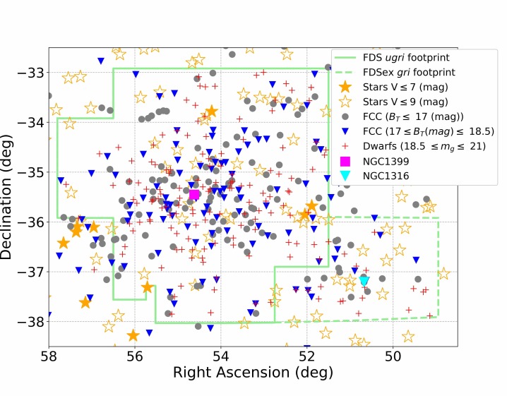
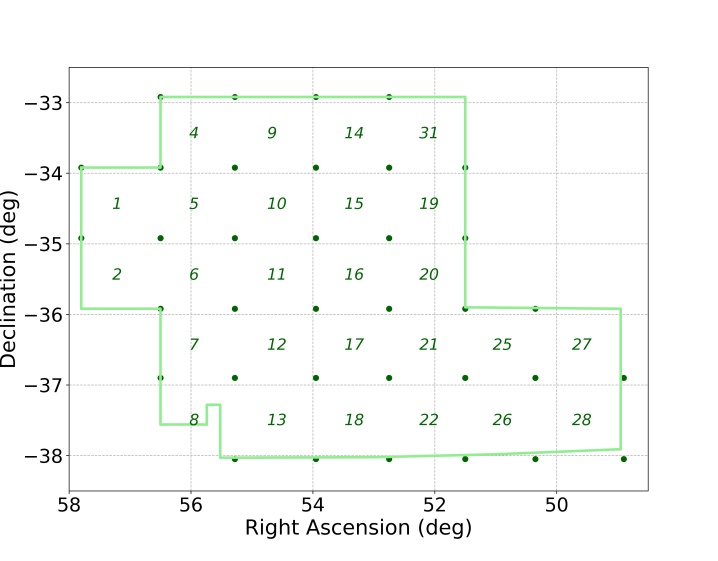
Figure 1: Left panel: The FDS footprint of the area covered by $ugri$ photometry (green solid line), and by only $gri$ (dashed green line). Other sources from catalogs available in the literature are also shown, as labeled. Bright galaxies from the Fornax Cluster Catalog (Ferguson, 1989) are subdivided into two categories: likely members brighter than $B_{T}=17$ mag and with $17\leq B_{T}\leavevmode\nobreak\ (mag)\leq 18.5$ (filled gray circles and blue triangles, respectively; from Ferguson, 1989, Table II). Dwarf galaxies from FDS by Venhola et al. (2018), in the magnitude range $18.5\leq m_{g}\leavevmode\nobreak\ (mag)\leq 21$, are indicated with red crosses. The positions of the two brightest galaxies, NGC 1316 and NGC 1399, are also shown with a filled cyan triangle and a magenta square, respectively. Orange filled/empty five pointed stars mark stars with $m_{V}\leq 7/\leq 9$ mag, respectively. Right panel: The FDS and FDSex area. Green lines mark the edges of the survey, green bullets show the edges of single pointings; the ID of the field is also indicated.

The data, data acquisition and reduction procedures are presented in a number of papers of the FDS series (Iodice et al., 2016, 2017a, 2017b, 2019; Venhola et al., 2017, 2018, 2019). A full description of the observations and the pipeline used for data reduction (AstroWISE, McFarland et al., 2013) steps are given in the cited papers, and in Peletier et al. (in prep.).

In what follows we describe two critical differences with respect to previous works, related to the focus on compact stellar systems in the present work.

2.2 Multi-band image stacks

The FDS standard reduction pipeline produced imaging data for many different scientific cases, with a general focus on extended galaxies in the cluster (e.g. Spavone et al., 2017). In columns (2-5) of Table 1, we report the median full width at half maximum, FWHM, of the point spread function, PSF, in arcseconds for each FDS VST field and for each available band; the FWHM distributions are also shown in the histograms of Figure 2. The large FWHM variation, up to $\sim 50\%$ for different fields observed in the same passband, may represent a limitation to the effectiveness of the FDS dataset for the science cases related to compact objects (foreground MW stars, background galaxies, GCs host in Fornax, etc.). The typical FWHM scatter of the exposures combined to obtain the single FDS fields stacks is $rms_{MAD}=0\aas@@fstack{\prime\prime}36,\leavevmode\nobreak\ 0\aas@@fstack{\prime\prime}21,\leavevmode\nobreak\ 0\aas@@fstack{\prime\prime}33,\leavevmode\nobreak\ 0\aas@@fstack{\prime\prime}21$ in $u/g/r/i$-band, respectively.

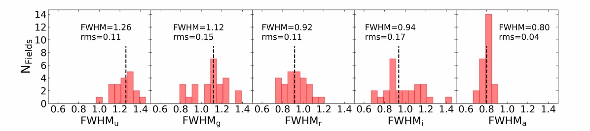
Figure 2: Histograms of the median PSF FWHM of the FDS fields in the four available passbands, plus the multi-band $a$-stacks. The vertical dashed line shows the median of the ensemble.

To improve the detection and characterization of compact sources, we combined in a single coadded image all single VST exposures in $g$, $r$ and $i$ bands with a median FWHM lower than a fixed upper limit, $u$-band exposures were ignored because of the lower signal-to-noise and worse FWHM. After various experiments, we fixed the FWHM limit to $0\aas@@fstack{\prime\prime}9$: if a lower FWHM cut is adopted, the final resolution of the stack improves, at the expenses of a worse detection limit and larger field-to-field mean FWHM variability; a higher FWHM cut, instead, would make ineffective the use of multi-band stacks compared to single bands images. Hence, the $0\aas@@fstack{\prime\prime}9$ cut is adopted as the trade off between needs of better resolution and uniformity of the master detection frame. The combined image was processed as the single band images, except for the photometric calibration which is not derived. In the following, we refer to the coadd of $gri$ exposures with FWHM cut as $a$-stack, and use the subscript $a$ to identify the quantities derived from it. With this procedure, a new frame with narrower and more stable FWHM compared with $ugri$ bands is obtained, and used as master detection frame. This improved both the uniformity of detections over the different FDS fields, and the determination of the morphological properties of the sources, allowing more accurate characterization of compact and point-like objects. These $a$-stacks will not be used to define absolute quantities (like calibrated magnitudes), but only for relative ones (like the $CI_{n}$, see below), thus the wavelength dependence of the PSF and source morphology will not be an issue.

As shown in Table 1, the $a$-stacks have a median FWHM smaller by $\sim 15\%$ and with an $rms$ scatter a factor of $\sim 2.5$ lower than the median and $rms$ of the FWHM for the best passband, namely the $r$-band.

In Figure 3 we show a $1\arcmin\times 1\arcmin$ thumbnail of the same FDS region in $g$, $r$, and $i$-band and the $a$-stack image centered on background spiral galaxy in the field FDS#5 ($FCCB\,1532$, Ferguson, 1989). In general, the depth of the coadded multiband $a$-stack does not change much compared with the best band of the field, because the reduced number of exposures used is compensated by the better S/N due to the higher spatial resolution. The spatial resolution, however, is in all cases enhanced, as shown in the $FWHM_{a}$ column in Table 1.

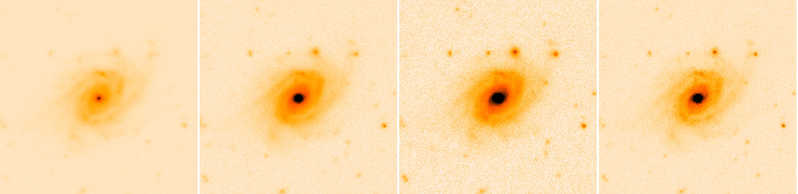
Figure 3: From left to right: $g$, $r$, $i$-band and $a$-stack of a background spiral galaxy in the field FDS#5 ($FCCB\,1532$, Ferguson, 1989). The rightmost panel is derived from the combination of the sub-exposures of the first three panels, selecting only the ones with lowest atmospheric turbulence (see text).

Table 1: Image quality parameters for FDS and FDSex fields

Field ID	$FWHM_{u}$	$FWHM_{g}$	$FWHM_{r}$	$FWMH_{i}$	$FWHM_{a}$	$\langle P_{2}(s)\rangle$	$\sigma[P_{2}(s)]$	$\langle P_{2}(w)\rangle$	$\sigma[P_{2}(w)]$	$\langle P_{2}(x)\rangle$	$\sigma[P_{2}(x)]$	$u_{lim}$	$g_{lim}$	$r_{lim}$	$i_{lim}$
	$(\arcsec)$	$(\arcsec)$	$(\arcsec)$	$(\arcsec)$	$(\arcsec)$	(mag)	(mag )	(mag)	(mag)	(mag)	(mag)	(mag)	(mag)	(mag)	(mag)
(1)	(2)	(3)	(4)	(5)	(6)	(7)	(8)	(9)	(10)	(11)	(12)	(13)	(14)	(14)	(16)
1	1.17 $\pm$ 0.03	1.35 $\pm$ 0.12	1.14 $\pm$ 0.11	0.69 $\pm$ 0.08	0.72 $\pm$ 0.08	0.006	0.019	0.018	0.024	0.014	0.030	24.24$\pm$ 0.13	25.39$\pm$ 0.10	24.65 $\pm$0.17	24.53 $\pm$0.15
2	1.21 $\pm$ 0.08	1.11 $\pm$ 0.16	0.89 $\pm$ 0.05	0.79 $\pm$ 0.09	0.79 $\pm$ 0.04	0.008	0.018	0.011	0.020	0.005	0.032	24.02$\pm$ 0.18	25.41$\pm$ 0.13	25.04 $\pm$0.12	24.12 $\pm$0.13
4	1.19 $\pm$ 0.05	1.39 $\pm$ 0.13	1.19 $\pm$ 0.09	0.70 $\pm$ 0.07	0.71 $\pm$ 0.07	0.007	0.020	0.052	0.026	-0.005	0.029	24.12$\pm$ 0.09	25.35$\pm$ 0.10	24.65 $\pm$0.11	24.44 $\pm$0.14
5	1.35 $\pm$ 0.07	1.17 $\pm$ 0.14	0.98 $\pm$ 0.06	1.11 $\pm$ 0.16	0.82 $\pm$ 0.09	0.005	0.018	0.007	0.024	0.012	0.033	24.05$\pm$ 0.17	25.48$\pm$ 0.10	24.72 $\pm$0.08	23.88 $\pm$0.10
6	1.13 $\pm$ 0.07	0.83 $\pm$ 0.04	1.08 $\pm$ 0.12	1.24 $\pm$ 0.14	0.80 $\pm$ 0.05	0.005	0.021	0.023	0.023	-0.007	0.033	24.22$\pm$ 0.10	25.70$\pm$ 0.10	24.66 $\pm$0.14	23.51 $\pm$0.09
7	1.03 $\pm$ 0.06	0.82 $\pm$ 0.04	0.90 $\pm$ 0.07	1.44 $\pm$ 0.13	0.78 $\pm$ 0.08	0.007	0.022	0.012	0.020	0.008	0.026	24.16$\pm$ 0.12	25.79$\pm$ 0.11	24.91 $\pm$0.13	23.35 $\pm$0.11
8	1.21 $\pm$ 0.10	0.93 $\pm$ 0.16	0.90 $\pm$ 0.12	0.96 $\pm$ 0.18	0.84 $\pm$ 0.13	0.006	0.021	0.022	0.024	-0.015	0.033	24.23$\pm$ 0.21	25.50$\pm$ 0.22	24.99 $\pm$0.21	23.72 $\pm$0.20
9	1.42 $\pm$ 0.08	1.20 $\pm$ 0.07	0.97 $\pm$ 0.08	0.84 $\pm$ 0.07	0.82 $\pm$ 0.05	0.003	0.022	0.036	0.021	-0.015	0.035	23.96$\pm$ 0.09	25.50$\pm$ 0.12	25.06 $\pm$0.13	24.38 $\pm$0.13
10	1.34 $\pm$ 0.06	1.15 $\pm$ 0.05	0.96 $\pm$ 0.07	1.09 $\pm$ 0.11	0.86 $\pm$ 0.05	0.000	0.018	0.009	0.014	-0.010	0.026	24.09$\pm$ 0.10	25.52$\pm$ 0.09	24.84 $\pm$0.11	23.96 $\pm$0.11
11	1.27 $\pm$ 0.06	1.09 $\pm$ 0.14	1.08 $\pm$ 0.14	1.17 $\pm$ 0.10	0.84 $\pm$ 0.08	0.011	0.023	0.025	0.024	-0.002	0.032	24.09$\pm$ 0.13	25.22$\pm$ 0.10	24.65 $\pm$0.11	23.64 $\pm$0.09
12	1.18 $\pm$ 0.08	0.80 $\pm$ 0.04	0.97 $\pm$ 0.07	1.17 $\pm$ 0.09	0.80 $\pm$ 0.05	0.014	0.024	0.022	0.021	0.001	0.037	24.30$\pm$ 0.09	25.74$\pm$ 0.11	24.85 $\pm$0.11	23.61 $\pm$0.09
13	1.10 $\pm$ 0.05	0.91 $\pm$ 0.05	1.03 $\pm$ 0.08	1.16 $\pm$ 0.07	0.89 $\pm$ 0.05	0.003	0.016	0.021	0.016	-0.003	0.029	24.39$\pm$ 0.18	25.72$\pm$ 0.13	24.99 $\pm$0.12	24.22 $\pm$0.13
14	1.46 $\pm$ 0.09	1.18 $\pm$ 0.09	0.96 $\pm$ 0.08	0.85 $\pm$ 0.06	0.83 $\pm$ 0.06	0.004	0.019	0.012	0.017	0.005	0.028	23.99$\pm$ 0.08	25.43$\pm$ 0.12	24.94 $\pm$0.13	24.30 $\pm$0.12
15	1.30 $\pm$ 0.05	1.13 $\pm$ 0.04	0.88 $\pm$ 0.04	0.98 $\pm$ 0.09	0.81 $\pm$ 0.06	0.001	0.020	0.008	0.022	-0.001	0.031	24.19$\pm$ 0.11	25.37$\pm$ 0.09	25.10 $\pm$0.08	24.02 $\pm$0.16
16	1.31 $\pm$ 0.04	1.26 $\pm$ 0.08	0.91 $\pm$ 0.08	1.09 $\pm$ 0.07	0.84 $\pm$ 0.05	0.008	0.025	0.006	0.020	-0.000	0.035	24.16$\pm$ 0.11	25.31$\pm$ 0.08	24.93 $\pm$0.11	23.88 $\pm$0.09
17	1.27 $\pm$ 0.06	1.25 $\pm$ 0.16	0.82 $\pm$ 0.05	1.01 $\pm$ 0.07	0.80 $\pm$ 0.04	-0.006	0.020	0.020	0.020	-0.011	0.032	24.17$\pm$ 0.09	25.16$\pm$ 0.18	25.21 $\pm$0.11	24.01 $\pm$0.10
18	1.12 $\pm$ 0.08	0.94 $\pm$ 0.05	1.03 $\pm$ 0.07	1.12 $\pm$ 0.12	0.87 $\pm$ 0.09	-0.002	0.018	0.021	0.016	0.007	0.025	24.19$\pm$ 0.23	25.57$\pm$ 0.13	24.93 $\pm$0.12	24.14 $\pm$0.13
19	1.26 $\pm$ 0.05	1.14 $\pm$ 0.09	0.89 $\pm$ 0.05	0.86 $\pm$ 0.06	0.79 $\pm$ 0.05	0.010	0.022	0.042	0.022	0.009	0.025	24.10$\pm$ 0.11	25.46$\pm$ 0.09	25.15 $\pm$0.10	24.13 $\pm$0.13
20	1.30 $\pm$ 0.05	1.23 $\pm$ 0.06	0.92 $\pm$ 0.09	1.08 $\pm$ 0.08	0.81 $\pm$ 0.08	0.019	0.033	-0.006	0.032	0.002	0.044	24.12$\pm$ 0.11	25.17$\pm$ 0.12	24.76 $\pm$0.13	23.80 $\pm$0.12
21	1.22 $\pm$ 0.05	1.12 $\pm$ 0.06	0.78 $\pm$ 0.05	0.88 $\pm$ 0.08	0.78 $\pm$ 0.04	0.001	0.022	0.004	0.027	0.002	0.035	24.06$\pm$ 0.11	25.22$\pm$ 0.09	24.92 $\pm$0.12	24.22 $\pm$0.09
22	…	1.03 $\pm$ 0.06	0.80 $\pm$ 0.06	0.85 $\pm$ 0.05	0.79 $\pm$ 0.05	…	…	0.004	0.019	0.007	0.029	…	25.27$\pm$ 0.14	24.92 $\pm$0.13	24.21 $\pm$0.10
25	…	1.12 $\pm$ 0.05	0.76 $\pm$ 0.06	0.85 $\pm$ 0.08	0.78 $\pm$ 0.08	…	…	0.016	0.025	-0.003	0.031	…	25.36$\pm$ 0.11	24.98 $\pm$0.12	24.10 $\pm$0.10
26	…	0.95 $\pm$ 0.12	0.80 $\pm$ 0.04	0.91 $\pm$ 0.08	0.78 $\pm$ 0.04	…	…	0.037	0.021	-0.018	0.035	…	24.79$\pm$ 0.15	25.00 $\pm$0.11	23.94 $\pm$0.13
27	…	1.05 $\pm$ 0.09	0.78 $\pm$ 0.06	0.89 $\pm$ 0.09	0.77 $\pm$ 0.08	…	…	0.012	0.026	-0.007	0.042	…	25.19$\pm$ 0.11	24.79 $\pm$0.15	23.75 $\pm$0.16
28	…	1.09 $\pm$ 0.07	0.79 $\pm$ 0.15	0.91 $\pm$ 0.11	0.78 $\pm$ 0.10	…	…	0.007	0.035	0.013	0.032	…	25.11$\pm$ 0.13	24.65 $\pm$0.19	23.78 $\pm$0.14
31	1.46 $\pm$ 0.08	1.22 $\pm$ 0.06	1.00 $\pm$ 0.07	0.86 $\pm$ 0.08	0.84 $\pm$ 0.05	0.012	0.022	0.030	0.023	0.003	0.032	23.83$\pm$ 0.11	25.31$\pm$ 0.11	24.78 $\pm$0.15	24.05 $\pm$0.17
Median	1.26$\pm$ 0.11	1.12$\pm$ 0.15	0.92 $\pm$ 0.11	0.94 $\pm$ 0.17	0.80 $\pm$ 0.04	0.006	0.021	0.017	0.022	0.000	0.032	24.12$\pm$ 0.13	25.38$\pm$ 0.17	24.92 $\pm$0.17	24.02 $\pm$0.24

2.3 Photometry and photometric calibration

Catalogs are derived for each single FDS pointing; the identification of fields with available data is shown in the right panel of Figure 1. To increase the contrast of faint sources close to the cores of extended galaxies, before running the procedures to obtain the photometry and the morphometry (like FWHM, elongation, flux radius, etc.; see section 2.4 below) we modeled and subtracted all Fornax members brighter than $B_{T}\sim 18$ mag. The fit of the isophotes is performed using the IRAF STSDAS task ELLIPSE, which is based on an algorithm by Jedrzejewski (1987).

To obtain the photometry of sources in FDS frames, we used a combination of procedures, based on SExtractor (Bertin & Arnouts, 1996) and DAOphot (Stetson, 1987) runs, and codes developed by the first author. We adopt AB mag photometric system, as in previous FDS works. The galaxy-subtracted frames used in this stage are already calibrated as described in the previous works of the FDS series (see below).

First, we used SExtractor to obtain the mean properties of each frame, like the FWHM; the reference morphometry for each source is obtained from the $a$-stacks, though we also derived the morphometric properties for all available passbands. Then, DAOphot is run on the $a$-stacks, and fed to our procedure to identify bright, non-saturated and isolated stars needed to obtain a variable PSF model over the single pointing. Typically, with this procedure we selected $\sim 200$ candidate PSFs per single FDS field, that were visually inspected in all bands to remove candidates contaminated by faint companions, bright halos of galaxies or saturated stars, or other instrumental artifacts. Using this iterative process, we ended up with a typical list of 50 to 100 point-like sources to model the PSF with DAOphot for each filter and field. The list of PSFs was then fed to DAOphot for PSF modeling, adopting the variable PSF option. The first complete DAOphot run was on the $a$-stack. The output table for this run was used to $i)$ identify sources to define a master detection catalog, $ii)$ obtain the DAOphot sharpness parameter, that will be used as additional parameter for selecting good candidate compact sources.

The master detection catalog was then given as input to run DAOphot on each available filter and for all fields: $ugri$ for the FDS area, $gri$ for FDSex.

We also run SExtractor on the full set of images, to obtain the aperture magnitude within 8-pixel diameter ($MAG\_APER$) and the automated aperture magnitude derived from Kron (1980) first moment algorithms ($MAG\_AUTO$), with the respective photometric errors. For the aperture magnitudes, after some tests we adopted the 8 pixel diameter: larger diameters implied larger statistical errors on derived magnitudes (because of the noisier background and higher contamination from neighboring sources), smaller diameters suffered from larger systematic errors (because larger aperture corrections are needed). Both $MAG\_APER(8)$ and $MAG\_AUTO$ are stored in our final catalogs; in particular $MAG\_AUTO$ provides a good choice for the magnitude of non-compact background objects.

The photometric calibration is carried out in two steps. The first is the same described in Venhola et al. (2018), and uses standard star fields observed each night and comparing their OmegaCAM magnitudes with the final data from the Sloan Digital Sky Survey Data III (Alam et al., 2015).

With such calibration, and after applying the field and pass-band dependent aperture corrections, the photometry of the same sources in different adjacent FDS pointings show a spatially variable offset, with a median upper limit of $\sim 0.1$ mag. This might be a consequence of the different (mean) photometric conditions for neighboring FDS fields during the FDS observing runs which span a time interval of $\sim 5$ years.

As a second step of the photometric calibration, to improve the photometric uniformity and consistency over the FDS (and FDSex) area, and to derive the spatially and filter dependent aperture correction map, we compared our VST photometry of bright non-saturated point-like sources to the APASS photometry and obtained the two-dimensional map that best matches the two datasets. The map is derived for each field separately, using a support vector machine (SVM) supervised learning method, with a radial basis function (RBF) kernel (Pedregosa et al., 2011). Only isolated unsaturated stars, brighter than a given magnitude cut (19/17/17/16.5 mag in $u/g/r/i$ band, respectively) are used in the regression algorithm.

The correction maps are derived from 200 to 300 stars per FDS field, the final median $rms_{VST-APASS}$ between VST and APASS photometry over the full set of re-calibrated frames is reported in Table 2. Figure 4 shows an example of the correction maps derived for the field FDS#19. Each correction map is then applied to its specific field and passband, to correct the photometry of all sources detected in the specific FDS pointing.

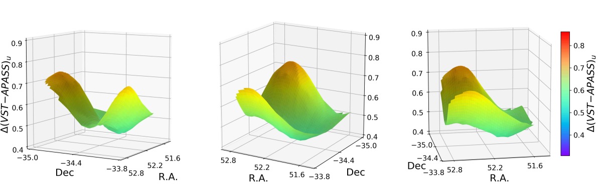
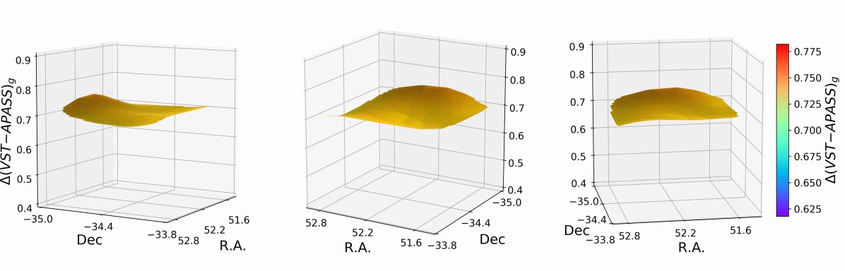
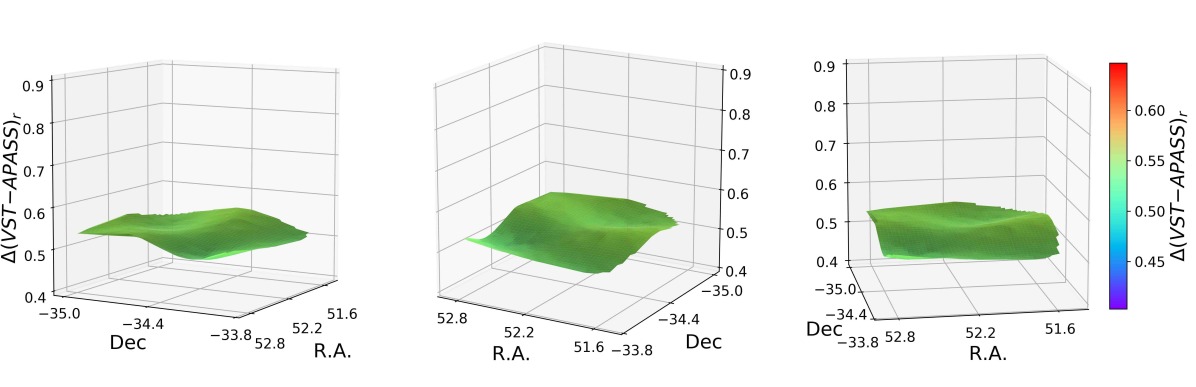
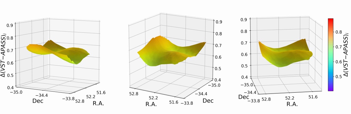
Figure 4: An example of the two-dimensional photometric correction maps for refining the photometry of FDS fields. The maps also include the aperture correction term. Field FDS#19 is shown: $u$, $g$, $r$ and $i$-band correction maps are plotted from upper to lower panels, respectively. For each passband the surface correction map is shown with the same color coding and for different viewpoints in each of the three panels.

Because APASS lacks $u$ coverage, for such passband we adopted a slightly different re-calibration strategy. After the preliminary calibration described above, the $B$-band magnitudes of stars from APASS were transformed to $u$-band using Lupton (2005) transformation equations available from the SDSS web pages. In particular: $u=B_{APASS}+0.8116\cdot(u{-}g)_{fit}-0.1313$, where the $(u{-}g)_{fit}$ color index is derived from the APASS $(g{-}i)$ and $(g{-}r)$ indices, using a second degree polynomial fit derived from SDSS data over different sky regions. From this stage on, by using the $u$-band magnitudes of stars in APASS derived as a function of the $B$, $g$, $r$, and $i$ photometry, we proceed to derive and apply the $u$-band correction maps as in $gri$ bands.

To further verify the validity of the calibration obtained with the strategy delineated above, especially for the more elaborate $u$-band, we matched and compared our photometry to the SkyMapper data (SM hereafter; Wolf et al., 2018; Onken et al., 2019). The SDSS photometric systems of APASS and SM are not equivalent, the $u$ and $g$ bands in particular show differences up to $0.5$ mag in the two systems (Wolf et al., 2018). However, within the color interval $\lvert g{-}i\rvert\leq 1$ mag, the SM to SDSS difference for $uri$-bands is $\ \raise-2.0pt\hbox{\hbox to0.0pt{\hbox{$\sim$}\hss}\raise 5.0pt\hbox{$<$}\ }0.1$ mag, while it is a factor of $\sim 4$ larger in $g$-band (Wolf et al., 2018, see their Figure 17 and sections 2.2, 5.4). Hence, as a further consistency check, we compare our VST re-calibrated photometry to SM data, within the color interval $\lvert g{-}i\rvert\leq 1$ mag.

Over the entire FDS area covered with $ugri$ observations, we found $\sim 46,500$ sources in common with SM. After identifying bright and isolated stars, and with the given prescriptions on $(g{-}i)$ color selection, the final sample contains $\sim 4,600$ objects ($\sim 220$ per FDS field).

Table 2 reports the median magnitude offsets between the FDS and SM photometry for the matched sources, together with the $rms$ derived from the median absolute deviation. With the only not unexpected exception of the $g$ band we find good agreement between the $u$, $r$ and $i$ photometry, with magnitude offsets better than 0.02 mag in $r$ and $i$ bands and of $\sim 0.05$ mag in $u$; the $rms_{MAD}$ is $\sim 0.03$ in $gri$ and about twice larger in $u$-band.

Table 2: FDS magnitudes compared with APASS and SM

Filter	$rms_{VST-APASS}$	$\Delta mag_{FDS-SM}$	$rms_{VST-SM}$
$u$	0.13	$-0.054$	0.066
$g$	0.03	$0.149$	0.031
$r$	0.05	$-0.015$	0.028
$i$	0.07	$-0.003$	0.025

For an independent check of the $g$-band photometry, we used the data from the HST/ACS Fornax Cluster Survey (ACSFCS, Jordán et al., 2007, 2015). In Figure 5 we report a comparison of our and ACSFCS $g$-band magnitudes. We matched the $\sim 6.300$ GC candidates from the ACSFCS with the FDSex $gri$ catalog, to avoid the worse completeness limit of the $u$-band in the $ugri$ catalogs. Adopting a matching radius of $1\aas@@fstack{\prime\prime}0$, a total of 3750 sources are found in common to both catalogs. The completeness of the matching is $\sim 90\%$ or higher at bright magnitudes ($m_{g}\leq 23$), decreases to $\sim 80\%$ for $m_{g}\leq 24$, and is lower than $\sim 70\%$ for $m_{g}\leq 25$. Hence, the completeness of the $gri$ catalog drops quickly below $m_{g}\sim 24.5$ (mag), which corresponds to $\sim$0.5 mag fainter than the turn over magnitude (TOM) of the GC luminosity function (GCLF) for galaxies in Fornax (Villegas et al., 2010).

The left panel of Figure 5 shows the VST to ACSFCS $g$-band magnitude difference versus $m_{g}$ (blue dots in the figure). From the matched catalog, we selected a reference GC sample (see next section), marked as red dots in the figure. The running mean difference for both the full matched sample and the reference sample are shown in the middle panel, adopting window bin size 100/50 for the full/best sample, respectively. Finally, the right panel of the diagram shows the same quantities as in the left one, but versus the $(g{-}i)$ color. In all cases shown, the difference is consistent with zero – $\Delta g(FDS{-}ACSFCS)={-}0.03\pm 0.12$ for the full sample of 3750 matched sources; $\Delta g(FDS{-}ACSFCS)={-}0.01\pm 0.07$ for the 1455 sources in the reference catalog – with no evidence of significant residual trends.

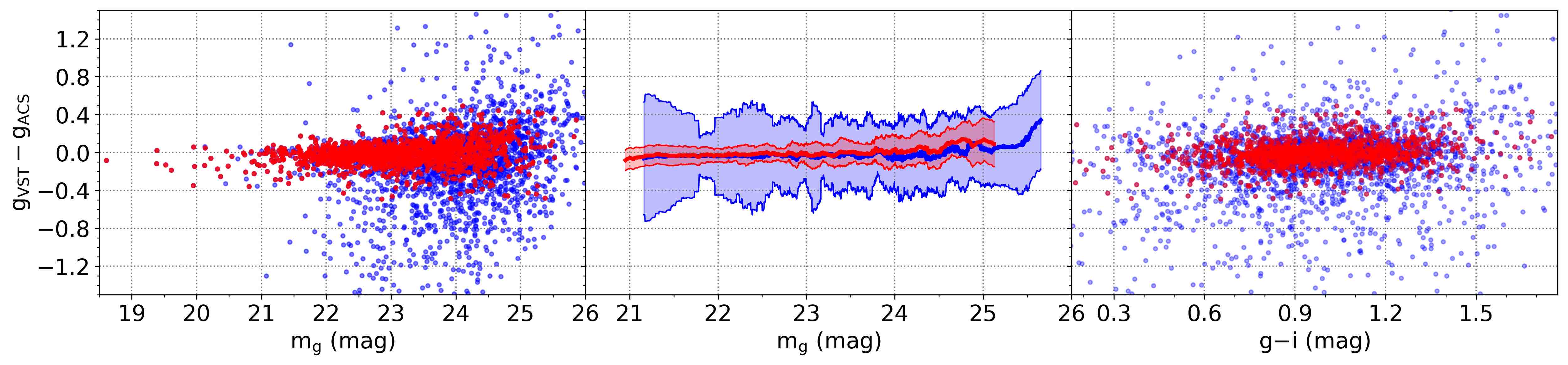
Figure 5: Left panel: $g$-band magnitudes from FDS compared with magnitudes of GC candidates from the ACSFCS. Blue symbols show the full matched set, red symbols identify compact sources in our reference catalog (see text). Middle panel: as left panel, but running averages are shown, with bin size of 100/50 objects for the blue/red symbols, respectively. Right panel: as left panel, but versus $(g{-}i)$ color.

2.4 Morphometry

As already anticipated in section §2.2: with morphometry we mean the measurement of all characteristics related to the shape of the source, our reference frames for the morphological characterization of sources are the multi-band $a$-stacks derived from $gri$ exposures with best seeing.

We put particular emphasis on deriving quantities useful for separating between point-like and extended sources, and identified a number of useful features: FWHM, CLASS_STAR, flux radius and elongation (major-to-minor axis ratio) derived with SExtractor, and the sharpness parameter derived from DAOphot.

For each source detected, we also measured the magnitude concentration index, described in Peng et al. (2011), defined as the difference in magnitude measured at two different radial apertures. After various tests we adopted as reference the concentration index derived from the $a$-stacks aperture magnitudes at 4 and 6 pixels: $CI=mag_{4\leavevmode\nobreak\ pix}-mag_{6\leavevmode\nobreak\ pix}$. For point-like sources, after applying the aperture correction to the PSF magnitudes of isolated stars at both radii, $CI$ should be statistically consistent with zero. The concentration index is constant for point-like objects, while extended sources have variable $CI$ larger than zero.

Because the $a$ is not a real photometric band, and because of the field-to-field variations, for simplicity we decided to normalize the CI index to 1, rather than to zero. The normalization was derived as follows: for each field we first estimated the CI from the magnitude difference within the two chosen apertures (so no aperture correction is applied), then derived the median CI of candidate point-like isolated and bright sources. Finally, the CI of the full sample was normalized to the median CI, such that compact sources should, by construction, be characterized by normalized CI values, $CI_{n}$, of $\sim 1$. Figure 6 shows the procedure described, for sources in the field FDS#13: as expected compact sources (here selected using the morphological parameters from SExtractor) occupy a flat sequence of constant $CI$ (left panel), normalized to one in the right panel of the figure.

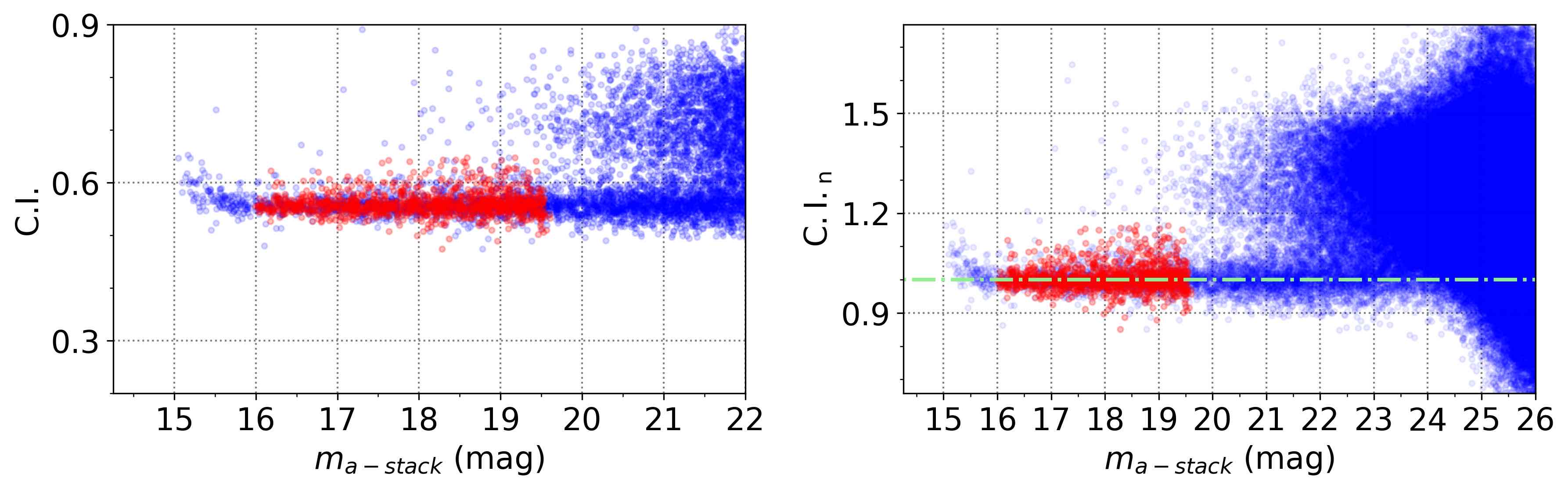
Figure 6: Normalization procedure for the CI, data for the field FDS#13 are shown. Left panel: concentration index $CI=mag_{4\leavevmode\nobreak\ pix}-mag_{6\leavevmode\nobreak\ pix}$ versus the uncalibrated $a$-stack magnitude. For sake of clarity, only the brightest magnitude range is shown. Blue dots refer to the full sample, red symbols to candidate compact sources used to derive the median $CI$ factor for normalization. Right panel: as left panel, but over a larger magnitude range, and after normalization to the median $CI$ of bright point-like sources (red dots). Point-like sources candidates are aligned along the sequence parallel to the $x$-axis, around $CI{{}_{n}}\sim 1$ (green dot-dashed line).

2.5 Final catalog and data quality

The DAOphot and SExtractor catalogs of sources in the FDS fields are finally combined in one single catalog (the same is done, independently, for the FDSex regions). The final catalog contains: $i)$ source identification adopting the IAU naming rules, and position from the $a$-stacks; $ii)$ the calibrated AB magnitudes from PSF photometry derived with DAOphot in all available bands; $iii)$ the uncorrected aperture and Kron-like magnitudes from SExtractor; $iv)$ the morphometric parameters for $a$-stacks (FWHM, CLASS_STAR, flux radius, elongation and sharpness) and for all other available bands.

The FDS catalog provides data based on the 21 FDS field in the $ugri$-bands, and for the $a$-stacks; a second $gri$-bands catalog for the full FDSex area is also generated.

In the catalogs, we include the extinction correction term, assuming the Galactic extinction values from the Schlafly & Finkbeiner (2011) recalibration of the Schlegel et al. (1998) infrared based dust maps.

Figure 7 shows a selection of extinction corrected color magnitude and color-color diagrams for the full sample of sources in the FDS catalog.

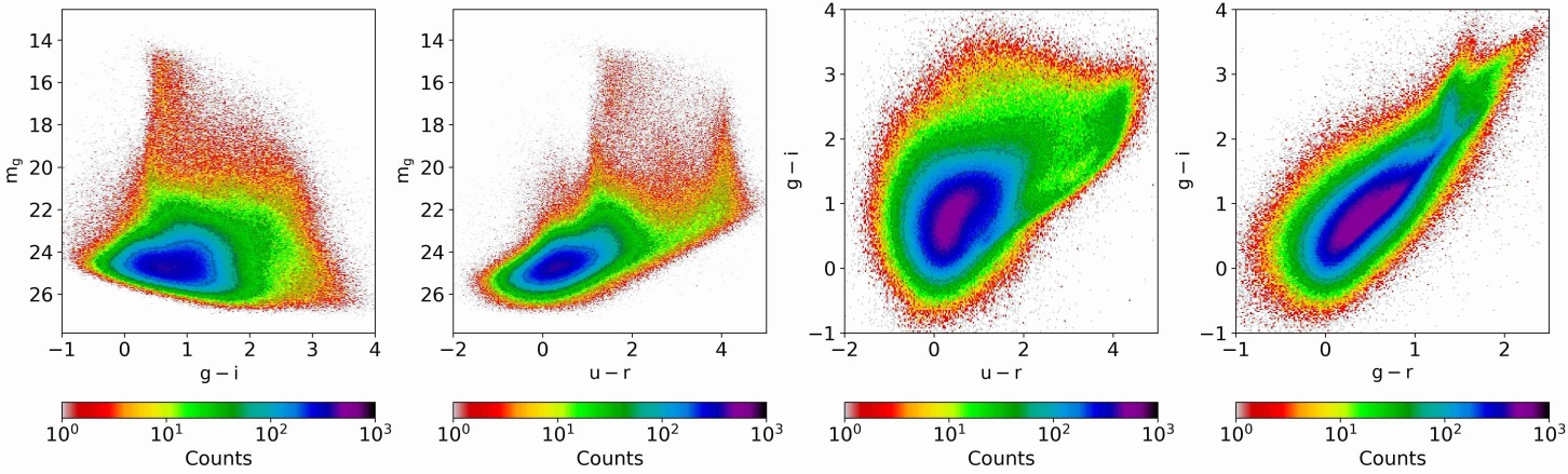
Figure 7: Hess color-magnitude and color-color diagrams of the full sample with $ugri$ photometry. Extinction corrected PSF magnitudes are used in all cases. FWHM is plotted in pixel units (the pixels scale is 0.2 arcsec/pixel).

As overall photometric quality assessment we used the principal colors, described in Ivezić et al. (2004). Principal colors are linear combinations of the SDSS colors of stars. We adopted the coefficients and selection parameters given in Tables 1-3 of Ivezić et al. (2004). The colors are combined to obtain a new color perpendicular to the stellar locus. Assuming the position of the locus to be fixed, the value of the principal colors is then an internal measure of the absolute photometric calibration of the data. Table 1 provides the median and $rms$ width of three principal colors, $P2(s)$, $P2(w)$ and $P2(x)$ for each FDS field; the median P2 values over the full set of fields is $<0.02$ with $rms\ \raise-2.0pt\hbox{\hbox to0.0pt{\hbox{$\sim$}\hss}\raise 5.0pt\hbox{$<$}\ }0.03$. The $P_{2}(s)$ depends on the $u$-band photometry, and cannot be determined over the FDSex fields. The overall $\langle P_{2}\rangle$ and $\sigma[P_{2}]$ values, and the values for each field, are consistent with the same value reported by Ivezić et al. (2004) for SDSS photometry.

Finally, we obtain the limiting magnitudes reported in Table 1 for all fields and bands, derived as $5\sigma$ magnitude integrated over the PSF, determined from the median S/N estimated as $\Delta m_{PSF}^{-1}$. The median $g$-band limiting magnitude is $g_{lim}\sim 25.4\pm 0.2$ mag; we note that the faintest GCs matched with the ACSFCS reach $m_{g}\sim 25.6$ mag, which increases to $m_{g}\sim 25.2$ mag for the sources in the reference catalog.

All catalogs are available via a dedicated web-interface of the FDS team, and are made available through the CDS. An extract of the data for the $\sim$1.7 million $ugri$ matched sources in the FDS catalog is reported in Table 3 (an extract for the $\sim$3.1 million sources in the FDSex $gri$ catalog is given in Table 4).

Table 3: An extract of the FDS $ugri$ catalog

ID	R.A. (J2000)	Dec. (J2000)	$m_{u}$	$m_{g}$	$m_{r}$	$m_{i}$	Star/Gal.	$CI_{n}$	F.R.	FWHM	Elong.	Sharp.	$E(B{-}V)$	Field
	(deg)	(deg)	(mag)	(mag)	(mag)	(mag)			(pixel)	(pixel)				(#)
(1)	(2)	(3)	(4)	(5)	(6)	(7)	(8)	(9)	(10)	(11)	(12)	(13)	(14)	(15)
FDSJ033744.66-345442.84	54.436077	-34.911900	21.550 $\pm$ 0.051	20.013 $\pm$ 0.053	19.172 $\pm$ 0.066	18.507 $\pm$ 0.059	0.029	1.449	12.57	13.84	1.260	4.559	0.011	10
FDSJ034014.64-345451.44	55.061020	-34.914288	21.675 $\pm$ 0.042	20.368 $\pm$ 0.039	19.509 $\pm$ 0.048	18.865 $\pm$ 0.037	0.029	1.266	7.37	12.47	1.670	3.240	0.012	10
FDSJ034028.79-345508.98	55.119957	-34.919163	18.585 $\pm$ 0.006	15.914 $\pm$ 0.005	14.790 $\pm$ 0.010	14.217 $\pm$ 0.006	0.996	1.040	3.25	4.56	1.010	0.872	0.012	10
FDSJ034055.30-345511.56	55.230427	-34.919880	24.431 $\pm$ 0.192	24.853 $\pm$ 0.124	24.014 $\pm$ 0.124	23.565 $\pm$ 0.154	0.830	1.243	3.44	7.99	1.570	0.920	0.011	10
FDSJ034044.55-345510.26	55.185608	-34.919518	25.478 $\pm$ 0.511	24.972 $\pm$ 0.116	24.841 $\pm$ 0.228	25.056 $\pm$ 0.507	0.512	1.304	2.26	3.45	1.700	1.218	0.011	10
FDSJ034036.60-345510.96	55.152508	-34.919712	24.901 $\pm$ 0.306	25.313 $\pm$ 0.171	25.395 $\pm$ 0.427	24.588 $\pm$ 0.348	0.562	0.659	1.67	2.00	1.340	-5.609	0.011	10
FDSJ034055.72-345510.38	55.232162	-34.919552	25.046 $\pm$ 0.358	24.225 $\pm$ 0.058	23.586 $\pm$ 0.074	22.863 $\pm$ 0.089	0.875	1.020	2.59	8.38	1.130	1.078	0.011	10
FDSJ034107.11-345506.88	55.279636	-34.918579	24.675 $\pm$ 0.284	25.149 $\pm$ 0.178	24.641 $\pm$ 0.258	24.698 $\pm$ 0.487	0.699	0.737	1.68	4.38	1.640	-6.010	0.011	10
FDSJ034015.36-345510.38	55.063984	-34.919552	25.319 $\pm$ 0.471	26.016 $\pm$ 0.316	24.720 $\pm$ 0.172	24.554 $\pm$ 0.457	0.430	1.082	2.10	3.79	1.200	-0.228	0.012	10
FDSJ033954.02-345511.46	54.975067	-34.919849	24.812 $\pm$ 0.326	24.716 $\pm$ 0.094	24.663 $\pm$ 0.168	23.768 $\pm$ 0.167	0.643	1.398	3.71	8.84	2.980	-1.337	0.012	10
FDSJ034037.01-345511.86	55.154224	-34.919960	24.901 $\pm$ 0.285	23.111 $\pm$ 0.026	22.269 $\pm$ 0.027	21.868 $\pm$ 0.038	0.980	0.956	2.69	4.55	1.080	-0.396	0.011	10
FDSJ033612.00-345454.11	54.050011	-34.915031	21.314 $\pm$ 0.059	20.323 $\pm$ 0.066	19.940 $\pm$ 0.081	19.444 $\pm$ 0.072	0.029	1.543	9.89	20.07	1.240	5.941	0.013	10

Table 4: An extract of the FDSex $gri$ catalog

ID	R.A. (J2000)	Dec. (J2000)	$m_{g}$	$m_{r}$	$m_{i}$	Star/Gal.	$CI_{n}$	F.R.	FWHM	Elong.	Sharp.	$E(B{-}V)$	Field
	(deg)	(deg)	(mag)	(mag)	(mag)			(pixel)	(pixel)				(#)
(1)	(2)	(3)	(4)	(5)	(6)	(7)	(8)	(9)	(10)	(11)	(12)	(13)	(14)
FDSJ033332.60-374029.36	53.385815	-37.674820	25.154 $\pm$ 0.127	25.010 $\pm$ 0.185	24.028 $\pm$ 0.175	0.566	1.169	3.21	10.39	1.130	1.797	0.011	18
FDSJ033343.98-374044.61	53.433262	-37.679058	20.012 $\pm$ 0.010	19.071 $\pm$ 0.006	18.451 $\pm$ 0.005	0.956	1.066	3.16	4.83	1.020	0.669	0.011	18
FDSJ033138.97-374012.90	52.912369	-37.670250	24.498 $\pm$ 0.077	23.868 $\pm$ 0.093	23.171 $\pm$ 0.140	0.015	1.228	3.55	9.99	1.490	2.733	0.016	18
FDSJ033539.47-374048.47	53.914478	-37.680130	23.700 $\pm$ 0.073	22.854 $\pm$ 0.054	22.144 $\pm$ 0.042	0.018	1.428	4.72	11.84	1.340	3.798	0.015	18
FDSJ033421.67-374037.64	53.590298	-37.677124	24.604 $\pm$ 0.093	24.398 $\pm$ 0.112	23.846 $\pm$ 0.190	0.125	1.307	3.23	9.30	1.370	2.152	0.013	18
FDSJ033258.65-374024.76	53.244354	-37.673546	24.396 $\pm$ 0.074	24.348 $\pm$ 0.105	24.330 $\pm$ 0.232	0.457	1.111	2.50	6.21	1.120	0.839	0.015	18
FDSJ033118.49-374009.10	52.827042	-37.669193	24.306 $\pm$ 0.083	23.514 $\pm$ 0.075	22.892 $\pm$ 0.088	0.012	1.374	4.59	15.56	1.330	4.176	0.016	18
FDSJ033216.89-374016.07	53.070377	-37.671131	25.622 $\pm$ 0.183	24.934 $\pm$ 0.170	24.127 $\pm$ 0.226	0.474	1.368	2.91	5.70	1.310	2.713	0.016	18
FDSJ033258.88-374023.19	53.245346	-37.673107	25.225 $\pm$ 0.144	25.426 $\pm$ 0.294	25.130 $\pm$ 0.500	0.513	1.013	1.86	4.39	2.190	-1.384	0.015	18
FDSJ033211.86-374023.13	53.049416	-37.673092	24.437 $\pm$ 0.096	22.781 $\pm$ 0.057	21.589 $\pm$ 0.063	0.001	1.441	6.47	19.87	1.390	4.409	0.015	18
FDSJ033157.13-374013.28	52.988060	-37.670353	25.117 $\pm$ 0.144	24.759 $\pm$ 0.180	24.338 $\pm$ 0.269	0.559	1.473	4.00	8.01	1.700	3.462	0.015	18
FDSJ033107.58-374005.39	52.781567	-37.668163	24.658 $\pm$ 0.083	23.182 $\pm$ 0.051	22.461 $\pm$ 0.063	0.798	1.112	2.92	7.75	1.330	1.349	0.016	18

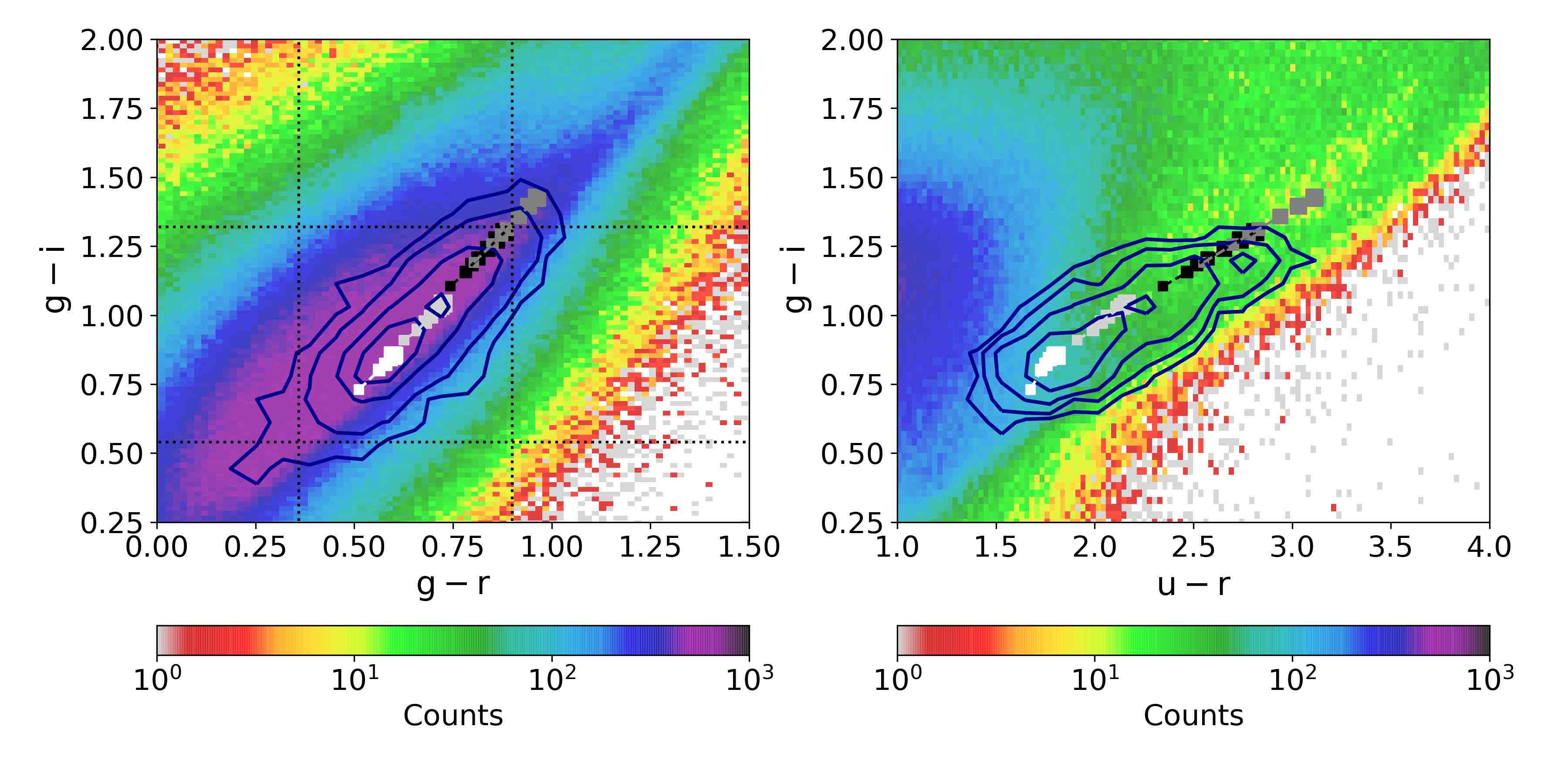
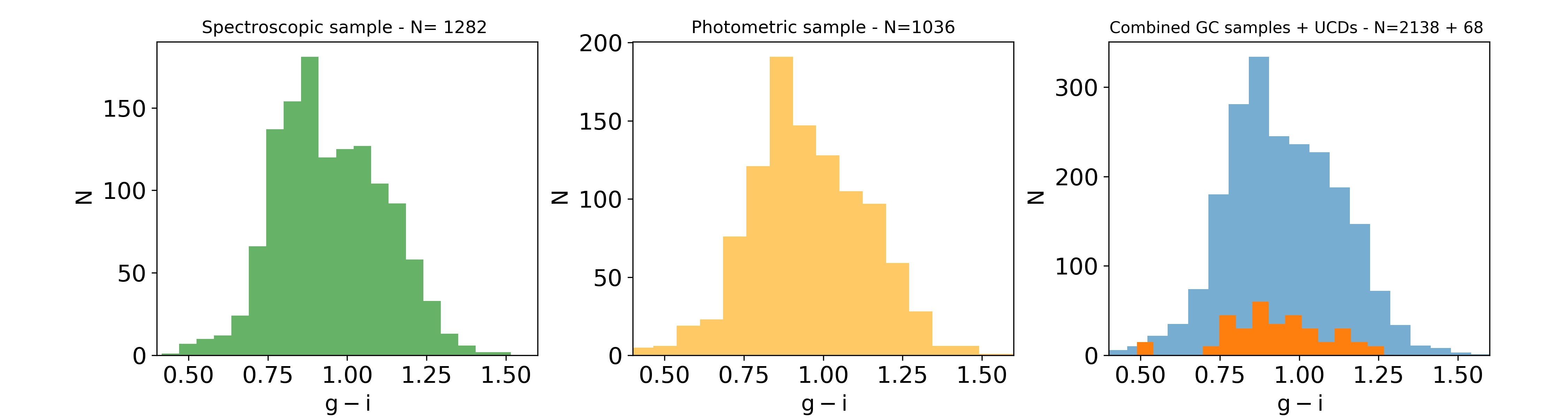
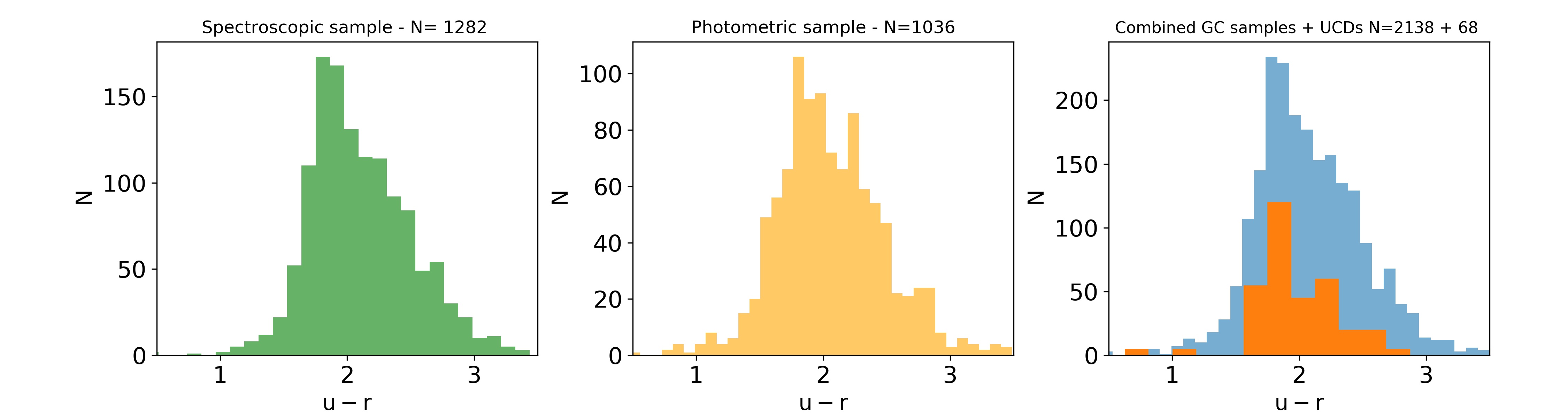
Figure 8: Upper panels: Color-color Hess diagrams for the sample of sources with $ugri$ photometry, over the color interval expected for GCs and UCDs. The dark-blue lines show the linear spaced contour levels of sources in the master GC catalog. Filled squares show the integrated colors from the SPoT stellar population synthesis code. White, light-gray, black and dark-gray symbols indicate metallicity $[Fe/H]$ =[-1.3, -0.7, 0.0, 0.4] respectively; symbols size scales with increasing model age, ranging between 4 and 14 Gyr, with 2 Gyr step. Same metallicity models are connected with dashed lines. In the left color-color panel we also draw with dotted lines the color intervals of GCs assuming $\pm 3{-}rms_{MAD}$ with respect to the median values in Table 7. Middle and lower panels: $(g{-}i)$ and $(u{-}r)$ color histograms, respectively, for the master spectroscopic (left panel, green histogram), photometric (middle, yellow), and combined (right, blue) GC catalogs. In the third histograms the data of UCDs are also shown (orange), expanded by a factor of five for sake of clarity. Only sources brighter than $m_{g}=23.5$ mag are considered.

3 A preliminary map of GCs and UCD galaxies over the FDS area

One of the goals of the FDS survey is to map the distribution of GCs and UCDs in Fornax out to the virial radius. In the following sections, and –more in details– in a forthcoming dedicated paper (Cantiello et al., 2020, in prep.) we analyze and discuss the cluster-wide properties of these two classes of compact stellar systems, with more emphasis on GCs.

Unambiguously identifying GCs from purely optical photometry is unfeasible. In Cantiello et al. (2018b) we showed that also spectroscopic samples might be affected by non negligible contamination. Muñoz et al. (2014) demonstrated that optical data including the $u$ band, combined with $K$-band near-IR data can dramatically reduce the contamination by fore/background sources.

Lacking a publicly available deep near-IR survey covering the FDS area, we proceed as already done in our previous works on GCs from the VEGAS and FDS surveys (Cantiello et al., 2015; Cantiello, 2016; Cantiello et al., 2018a; D’Abrusco et al., 2016).

Briefly, we identify a master catalog of GCs, and UCDs, and use the main properties of confirmed sources to constrain the mean loci of several photometric (magnitudes, colors, etc.) and morphometric ($CI_{n}$, galaxy/star classification, etc.) indicators.

In the following section we discuss the procedures adopted for identifying the loci of GCs using several parameters.

3.1 GCs & UCDs Master Catalogs

We define a master catalog of GCs and UCDs taking as reference literature spectroscopic and photometric studies, adopting $M_{g}=-10.5$ mag as GC/UCD separation criteria, corresponding to $M_{V}\sim-11$ mag ($\sim 10^{7}M_{\odot}$), and to an apparent $m_{g}=21$ magnitude at the adopted distance to Fornax (e.g. Mieske et al., 2004; Hilker et al., 2007). We collect photometric data from the already mentioned ACSFCS survey (Jordán et al., 2007, 2015). The advantage of ACS with respect to other imagers, is the very high resolution allowed by the space-based observations. At the distance of Fornax, GCs observed with the ACS camera appear as partially resolved sources, so their physical size can be estimated and used as a further parameter to reliably separate them from foreground stars and background galaxies. From the ACSFCS GC sample, we selected only GC candidates with high probability $p_{GC}$ of being a GC ($p_{GC}\geq 0.75$, derived according to a maximum-likelihood estimate, Jordán et al., 2009).

The spectroscopic sample is a combination of Pota et al. (2018) and Schuberth et al. (2010) datasets. By matching the spectroscopic and photometric catalogs –cleaned up by the common sources– with our FDS $ugri$ catalog, we obtained a list of $\sim$3.250 GCs.

We complete our master catalogs of reference compact stellar systems with 68 bright sources in Fornax, confirmed UCD compiled from the available spectroscopic and photometric literature for this class of objects in Fornax.

The GC and UCD master catalogs are given in the Table 5 and 6.

The upper panels in Figure 8 shows the same color-color diagrams as in Figure 7 with a zoom over the color-color region of GCs and UCDs. The contour levels of sources from the master catalog are reported with thick dark-blue lines (we adopt linear spacing for contour levels). In the figure we also report the SPoT simple stellar population models (Brocato et al., 1999; Cantiello et al., 2003; Raimondo et al., 2005), for an age range of 4-14 Gyr and metallicity $[Fe/H]$ =-1.3 to 0.4 dex. The consistency between the empirical loci of GCs and stellar population models for the typical age and metallicity ranges of GCs, provides further independent support to the reliability of the calibration approach adopted. In the $(u{-}r)$ -$(g{-}i)$ plane, the most metal-rich old stellar population models do not match with the observed GC distribution. One possible explanation is the combination of two effects: the small number of observed old GCs with such high metallicity (age$\geq 10$ Gyr, [Fe/H]$\ =0.4$, more than twice solar metallicity), and, consequently, the uncertainties of stellar population models is this regime.

The middle and lower panels of the figure also show the $(g{-}i)$ and $(u{-}r)$ color histograms for the photometric, spectroscopic and combined samples, for sources brighter than $m_{g}=23.5$ mag. The asymmetric appearance of the color distribution is a consequence of the well-known color bimodality of GC systems in some filters (Ashman & Zepf, 1992; Yoon et al., 2006; Blakeslee et al., 2010; Usher et al., 2012; Cantiello et al., 2014), here smoothed as the GC sample is a combination of GCs around $\sim 30$ galaxies in Fornax, each one with different morphological types and magnitudes, hence with different properties in terms of GCs color peaks (Peng et al., 2006).

Table 5: Master catalog of GCs

ID	R.A. (J2000)	Dec. (J2000)	$m_{u}$	$m_{g}$	$m_{r}$	$m_{i}$	Star/Gal.	$CI_{n}$	F.R.	FWHM	Elong.	Sharp.	$E(B{-}V)$	Field	FCC	$p_{GC}$	$r_{h}$	Source
	(deg)	(deg)	(mag)	(mag)	(mag)	(mag			(pixel)	(pixel)				(#)			(arcsec)
(1)	(2)	(3)	(4)	(5)	(6)	(7)	(8)	(9)	(10)	(11)	(12)	(13)	(14)	(15)	(16)	(17)	(18)	(19)
FDS032625.46-354235.74	51.606079	-35.709927	24.917(0.449)	23.694(0.059)	22.952(0.047)	22.718(0.095)	0.887	1.048	2.26	5.64	1.14	0.565	0.01	20	47	1.0	0.243	P
FDS032626.39-354229.81	51.609943	-35.708279	24.595(0.336)	22.749(0.022)	22.013(0.025)	21.688(0.037)	0.981	0.998	2.61	4.32	1.12	0.141	0.01	20	47	1.0	0.275	P
FDS032627.14-354245.15	51.613079	-35.712543	24.001(0.213)	22.418(0.02 )	21.774(0.019)	21.528(0.036)	0.983	1.039	2.44	4.24	1.04	0.304	0.01	20	47	1.0	0.281	P
FDS032627.18-354357.56	51.613262	-35.732655	23.739(0.139)	22.258(0.017)	21.39 (0.015)	21.144(0.024)	0.962	1.017	2.6	4.25	1.06	0.387	0.01	20	47	1.0	0.313	P
FDS032627.23-354125.68	51.613449	-35.690468	24.354(0.238)	23.268(0.039)	22.535(0.031)	22.367(0.065)	0.982	1.101	2.58	4.75	1.06	0.665	0.01	20	47	1.0	0.317	P
FDS032627.27-354237.98	51.613628	-35.710552	24.623(0.332)	24.115(0.083)	23.461(0.074)	23.201(0.124)	0.746	1.056	2.7	6.41	1.17	1.172	0.01	20	47	0.95	0.47	P
FDS032627.38-354224.34	51.614079	-35.70676	24.743(0.404)	23.363(0.039)	22.779(0.039)	22.535(0.078)	0.979	1.029	2.63	5.02	1.13	0.603	0.01	20	47	0.98	0.529	P
FDS032627.66-354441.02	51.615265	-35.744728	23.791(0.134)	22.496(0.02 )	21.671(0.018)	21.459(0.029)	0.982	0.987	2.51	4.14	1.05	0.082	0.01	20	47	1.0	0.283	P
FDS032628.10-354356.31	51.617069	-35.732307	24.739(0.291)	23.323(0.039)	22.408(0.032)	22.218(0.059)	0.977	1.036	2.35	4.55	1.05	0.235	0.01	20	47	1.0	0.356	P
FDS032628.17-354359.17	51.617355	-35.733105	25.015(0.486)	23.795(0.058)	23.191(0.055)	22.928(0.086)	0.177	1.637	5.3	16.93	1.43	1.453	0.01	20	47	0.98	0.37	P
FDS032628.20-354425.43	51.617496	-35.740398	24.222(0.194)	24.278(0.081)	23.706(0.095)	23.046(0.113)	0.656	1.115	2.65	7.61	1.21	0.613	0.01	20	47	0.97	0.218	P
FDS032628.34-354341.85	51.618095	-35.728291	25.107(0.395)	24.443(0.102)	23.598(0.075)	23.546(0.185)	0.8	1.048	2.49	5.77	1.14	0.581	0.01	20	47	0.99	0.294	P
…
FDS033633.14-345643.64	54.138096	-34.945457	23.595(0.142)	22.007(0.013)	21.226(0.014)	20.954(0.016)	0.921	1.007	2.76	4.29	1.08	0.341	0.015	11	…	…	…	S
FDS033633.49-350248.19	54.139542	-35.046719	24.75 (0.418)	22.906(0.031)	22.175(0.027)	21.732(0.045)	0.984	1.013	2.5	4.39	1.03	0.27	0.014	11	…	…	…	S
…
FDS033630.08-350013.69	54.125324	-35.003803	24.466(0.393)	22.079(0.014 )	21.266(0.016)	20.862(0.021)	0.926	1.054	2.81	4.75	1.1	0.486	0.015	11	167	1.0	0.381	S+P
FDS033630.10-351753.79	54.125427	-35.298275	22.792(0.066)	21.364(0.009 )	20.771(0.012)	20.453(0.019)	0.911	1.084	3.3	5.18	1.53	0.489	0.011	11	170	1.0	0.468	S+P

Table 6: Master catalog of UCDs

ID	R.A. (J2000)	Dec. (J2000)	$m_{u}$	$m_{g}$	$m_{r}$	$m_{i}$	Star/Gal.	$CI_{n}$	F.R.	FWHM	Elong.	Sharp.	$E(B{-}V)$	Field	$v_{hel}$	Source
	(deg)	(deg)	(mag)	(mag)	(mag)	(mag			(pixel)	(pixel)				(#)	(km/s)
(1)	(2)	(3)	(4)	(5)	(6)	(7)	(8)	(9)	(10)	(11)	(12)	(13)	(14)	(15)	(16)	(17)
FDS033854.05-353333.42	54.725212	-35.559284	20.701(0.037)	18.959 (0.042)	18.037(0.041)	17.626(0.036)	0.029	1.321	6.05	7.77	1.04	3.393	0.01	11	1517.0 (6.0)	F08
FDS033805.05-352409.33	54.521023	-35.402592	21.056(0.015)	19.308 (0.007)	18.568(0.009)	18.238(0.007)	0.959	1.024	2.99	4.52	1.13	0.559	0.012	11	1198.9 (6.1)	F08
FDS033935.92-352824.59	54.899654	-35.473499	21.109(0.022)	19.673 (0.027)	19.033(0.022)	18.588(0.013)	0.261	1.163	3.78	5.31	1.06	1.585	0.011	11	1878.0 (5.0)	B07
FDS033806.29-352858.72	54.526222	-35.482979	21.447(0.022)	19.814 (0.017)	19.086(0.022)	18.681(0.014)	0.799	1.137	3.59	5.39	1.26	1.335	0.011	11	1234.0 (5.0)	B07
FDS033703.22-353804.51	54.263435	-35.634586	21.66 (0.025)	19.895 (0.015)	19.12 (0.018)	18.699(0.013)	0.537	1.123	3.61	4.94	1.03	1.482	0.011	11	1561.0 (3.0)	F08
FDS033810.34-352405.79	54.543095	-35.401608	21.653(0.019)	19.987 (0.005)	19.261(0.005)	18.972(0.005)	0.979	0.985	2.71	4.18	1.09	0.131	0.012	11	1626.0 (10.0)	M08
FDS033952.54-350424.04	54.968903	-35.073345	21.342(0.023)	20.018 (0.019)	19.332(0.014)	19.069(0.018)	0.863	1.073	3.71	4.63	1.06	0.955	0.011	11	1236.0 (21.0)	F08
FDS033823.72-351349.49	54.59885	-35.230415	21.515(0.02 )	20.13 (0.007)	19.579(0.01 )	19.308(0.013)	0.831	1.117	3.12	4.74	1.02	1.129	0.012	11	1637.0 (14.0)	F08
FDS033743.56-352251.47	54.431484	-35.380966	21.616(0.025)	20.16 (0.007)	19.592(0.014)	19.271(0.011)	0.764	1.093	3.23	4.81	1.07	1.214	0.013	11	1420.0 (7.0)	F08
FDS033841.94-353313.03	54.674747	-35.553619	21.944(0.025)	20.194 (0.01 )	19.462(0.008)	19.091(0.007)	0.967	1.051	2.86	4.47	1.04	0.578	0.01	11	2024.0 (10.0)	M08
FDS033627.70-351413.84	54.115421	-35.237179	22.214(0.046)	20.198 (0.009)	19.36 (0.02 )	18.925(0.02 )	0.803	1.171	3.45	5.55	1.14	1.385	0.012	11	1386.0 (4.0)	B07
FDS033920.51-351914.25	54.835464	-35.320625	21.916(0.032)	20.253 (0.02 )	19.562(0.025)	19.031(0.013)	0.176	1.174	3.61	5.37	1.03	1.905	0.011	11	1462.0 (5.0)	F08

3.1.1 GCs and UCDs Selection by shape & photometric properties

At the assumed distance of Fornax, our best resolution of $FWHM_{a}\sim 0\aas@@fstack{\prime\prime}7$ (e.g. field FDS#1 $a$-stack) corresponds to a physical size of $\sim 68$ pc. Using specific analysis tools (e.g. Baolab, Larsen, 1999), sources down to $\sim FWHM/10$, $\sim 7pc$ for us, are marginally resolved, and can be analyzed and identified as slightly resolved sources. Typical GC half light radii of 2-4 pc are found in Fornax GCs from high-resolution ACS data (Jordán et al., 2009; Masters et al., 2010; Puzia et al., 2014). Using as reference the catalog of Fornax GC candidates by Jordán et al. (2015), $\sim 0.5\%$ of the best sample ($p_{GC}\geq 0.75$) has an half light radius $r_{h}\geq 7$ pc estimated in both $g$ and $z$ bands. Hence, even at the best resolution, we can assume the largest fraction of GCs in our catalogs are indistinguishable from point like sources.

To identify compact stellar systems we adopted a procedure similar to our previous works (Cantiello et al., 2018a, b). We relied on several indicators of compactness derived from the multi-band $a$-stacks, as on such frames we have the lowest field-to-field variation, and -by construction- the best seeing over the entire FDS and FDSex areas. As in the previous works, we combined the selection based on $CI_{n}$ to other morphometric indicators from DAOphot and SExtractor (elongation, flux radius, FWHM, class star, sharpness). This refines and further cleans the final sample of compact sources by the possible outliers not identified by using the sole $CI_{n}$, or by any other single indicator.

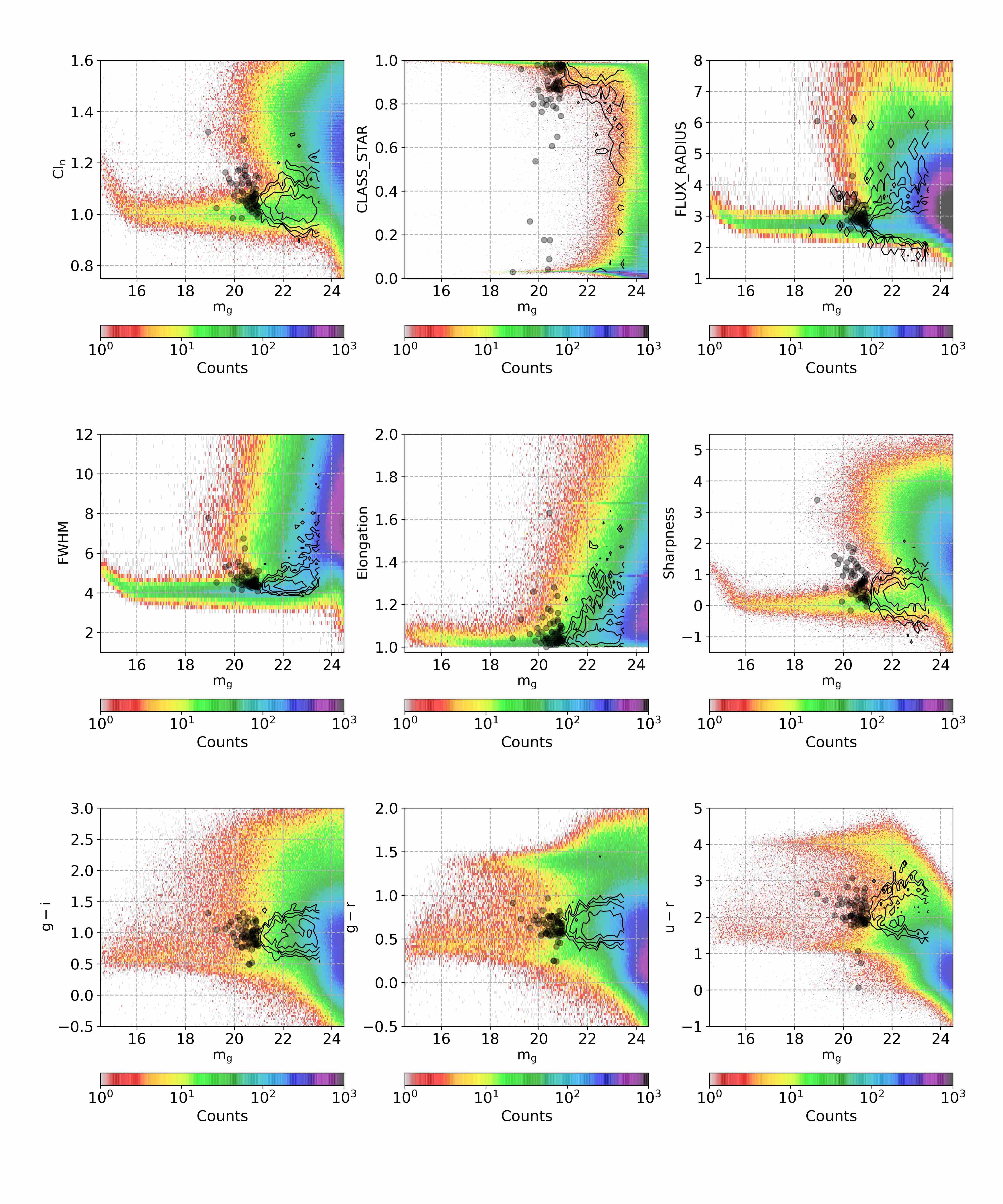
Figure 9: Hess diagrams of several morphometric and photometric indicators used to select GC candidates, with overlaid the contour levels of GCs in the master reference catalog, and UCDs (black circles).

A comparison of the $CI_{n}$ distribution for the full $ugri$ sample and for the GCs in the master catalog is shown in Figure 9 (upper left panel). From the comparison with the reference sample (dark contour levels in the panel) we find that the GC locus extends over the $CI_{n}\sim 1$ line, with a tail toward larger $CI_{n}$ values at fainter $m_{g}$ magnitudes. UCDs are also reported in the figure, with black filled dots, and show small but noticeable offsets with respect to the median properties of confirmed GCs, in particular for the size-dependent parameters (like flux radius and FWHM). Such an effect depends on the evidence that UCDs can have effective radii a factor of several times larger than GCs (Mieske et al., 2008; Misgeld & Hilker, 2011), i.e. they appear resolved, or slightly resolved, in our multi-band best seeing image stacks.

In Figure 9, we also show some of the other indicators used to identify GCs, together with UCDs and contour levels of the master catalog for the appropriate diagram.

To define the best GC selection intervals for each indicator, we analyzed the master catalog using GCs brighter than $m_{g}=23.5$, and derived the median and the $rms_{MAD}$ for each indicator. The results are reported in Table 7. In the table we also show the median properties for the reference sample of 68 UCDs.

Table 7: Median properties of the GCs and UCDs in the reference catalog

	GCs		UCDs
Indicator	Median	$rms_{MAD}$	Median	$rms_{MAD}$
$(g{-}i)$	0.93	0.13	0.94	0.12
$(g{-}r)$	0.63	0.09	0.64	0.08
$(u{-}r)$	2.02	0.26	2.03	0.21
$CI_{n}$	1.03	0.03	1.06	0.03
$CLASS\_STAR$	0.96	0.03	0.88	0.08
FWHM ($\arcsec$)	0.94	0.08	0.91	0.04
Flux Radius ($\arcsec$)	0.55	0.03	0.60	0.03
Elongation	1.09	0.05	1.04	0.02
Sharpness	0.32	0.26	0.69	0.34
$N_{sources}$	2138		68

In addition to morphology, we refine the catalog of candidate compact sources by their photometric characteristics: the shape of the GCLF (or the magnitude interval for known UCDs), the color intervals, and the errors on colors.

In our previous works, mostly focused on NGC 1399, we adopted as bright magnitude cut to the GCLF the magnitude $3\sigma_{GCLF}$ above the turn-over $m_{g}^{TOM}$ of this bright cD galaxy at the photo-center of Fornax. The Fornax cluster, with an estimated total line of sight depth of $\sim 2$ Mpc (Blakeslee et al., 2009), has member galaxies located at different physical distances. Adopting the ACSFCS results, the median $g$-band GCLF turn-over magnitude and $\sigma_{GCLF}$ values are $m_{g}^{TOM}=24.03\pm 0.15$ mag and $\sigma_{GCLF}=0.94\pm 0.11$ mag (Jordán et al., 2007). A $3\sigma_{GCLF}$ cut above the median TOM corresponds to $m_{g}\sim 21.2$ mag. For a rough estimate of the number of GCs lost with such bright cut level, we again take as reference the ACSFCS full list of GCs hosted by 43 Fornax galaxies (Jordán et al., 2015). The list contains 53 GCs brighter than $m_{g}=21.2$ mag ($\sim 0.8\%$ of the sample). Hence, in what follows we assume $m_{g}=21$ mag as bright cut of the GCLF, which includes 99.5% of the likely GCs sample in the ACSFCS sample. The bright cut helps having a sample of GC candidates with lower stellar contamination, at the cost of an expected minimal impact on the GC population. We will in any case also analyze candidates within $19.0\leq m_{g}\leq 21.0$ mag, the magnitude interval corresponding to UCDs in Fornax (Mieske et al., 2012). These systems share many characteristics with GCs but, as mentioned above, have larger effective radii than GCs (see Figure 9).

As maximum color uncertainty we choose $\Delta(g{-}i)_{max}=0.15$ and $\Delta(u{-}r)_{max}=0.3$, corresponding approximately to half of the separation between the blue and red peaks of the GCs color sub-populations host in typical bright galaxies (Cantiello et al., 2018a).

Thanks to the multiple color coverage, the selection of candidates can be improved using color-color criteria, rather than flat single-color ranges. The contour levels in the color-color diagrams of Figure 8 reveal relatively narrow color-color loci of GCs. A simple color-color selection box (e.g. black dotted lines in the upper left panel of the figure) would imply a trivial contamination from either stars or background objects. Instead, we proceed by inspecting in the color-color planes all sources satisfying the morpho-photometric parameters identified above. Finally, only the sources inside the color-color contours of the reference sample are identified as candidates and used for further analysis (see next section).

In summary, to identify the least contaminated and most complete possible GCs (and UCDs) catalog from our photometry, we adopted a three steps strategy. First, we generated a master GCs (and UCDs) catalog using confirmed sources in the literature. From the GCs catalog we cut out all sources fainter than $m_{g}=23.5$ mag, to better identify the morpho-photometric loci of GCs; the cut is adopted only for the reference catalog, for the GC identification and analysis on the FDS catalogs we will adopt a $\sim 1$ mag fainter limiting magnitude to increase the sample of GC candidates (see below). Second, we used the control parameters shown in Fig. 9, and the properties of the master catalogs to define the best intervals for GCs and UCDs selection. These selection criteria are then independently applied to the FDS and FDSex catalogs. For some parameters we adopted as confidence intervals the ranges from the master catalogs, using the $median\pm N\times rms_{MAD}$, with $N=4/2$ for GCs/UCDs respectively (median and $rms$ from Table 7); for the GCLF, colors, and color errors, we proceeded as described above. The complete list of parameters, together with the used ranges, is reported in Table 8. Third, the sample of compact sources after the previous steps was inspected in the color-color plane to further narrow down the contamination using the contour levels derived from the master catalog.

Table 8: Photometric and morphometric parameters adopted for source selections

	GCs		UCDs
Indicator	Min.	Max.	Min.	Max.
$m_{g}$	21.0	24.5	19.0	21.0
$(g{-}i)$	0.5	1.4	0.5	1.4
$(g{-}r)$	0.25	1.1	0.25	1.1
$(u{-}r)$	1.2	3.4	1.2	3.4
$CI\_n$	0.90	1.17	1.00	1.13
$CLASS\_STAR$	0.50	1.00	0.5	1.00
FWHM	0.61	1.26	0.8	1.12
Flux Radius	0.42	0.68	0.5	0.8
Elongation	$...$	1.30	$...$	1.5
Sharpness	-0.75	1.40	0.3	2.0
$\Delta$(g-i)	$...$	0.15	$...$	0.15
$\Delta$(u-r)	$...$	0.30	$...$	0.30

3.2 Surface distribution of compact sources over the FDS area

The analysis of the GCs over the FDS and FDSex area, together with the comparison with similar datasets, will be presented in more detail in a forthcoming paper. In what follows we show a preliminary determination of GCs and UCDs surface density maps as an example use of the FDS catalogs, based on the source selection strategies described in the previous section; in Section §4 we will also show an example of use of the catalogs for the study of background galaxies.

3.2.1 Globular clusters and UCDs distribution maps

Using the identification scheme described above, we inspect the GC distribution maps over the FDS and FDSex areas using as reference the $ugri$ and $gri$ selections, respectively.

GC candidates are derived by cross-matching the color-color regions of pre-selected GC candidates (Table 8), with the color-color loci of GCs identified in the master sample. Candidates falling in the contour levels of higher GCs density in the two-color diagram have higher likelihood of being true GCs. However, the narrow color-color range also implies lower completeness. In what follows, then, we analyze the GC density maps for candidates over different color-color contour levels.

Figure 10 shows the two-dimensional projected distribution over the $\sim 21$ sq. degree area of FDS. In the left panels of the figure we plot the color-color Hess diagrams of all sources identified with the selection criteria in Table 8, overplotting the contour levels of the GCs in the master sample. Even after all morpho-photometric cleaning of the sample (except for the color-color selection), a substantial fraction of selected candidates lies outside the expected GCs color-color region identified by the contour levels in the panel.

The middle and right panels of Figure 10 show the maps of GCs identified adding also the color-color contour level selection, i.e. of all sources falling in the contour levels marked in the left panels of Figure 10. Each row of panels in the figure refers to a different contour level, indicated by the thick magenta contour in the left panel. Again, the inner contours pinpoint regions with higher GCs density in the color-color diagram, thus the level of contamination from non-GCs decreases in the maps from the upper to lower panels in Figure 10; vice-versa, because of the smaller color-color intervals, lower panels suffer for higher incompleteness fractions. In particular, the lowermost panel is limited to a blue color-color region, hence mostly representative on the blue-GCs sub-population, also discussed below.

We calculate the smooth density maps using non-parametric kernel density estimates based on FFT convolution. After various tests, we adopted a grid mesh size of $\sim 0.1\arcmin$ spacing, smoothed with an Epanechnikov kernel, with kernel bandwidth five times the grid size.

Although obvious differences appear between GC maps drawn from the diverse color-color contour levels, there are several recurrent patterns appearing at various levels of selection, that is at different levels of GC contamination and incompleteness. The recurrence of the sub-structures over various GC color-color contours supports the reality of the sub-structure itself. Some of these patterns were also discussed in our works (D’Abrusco et al., 2016; Cantiello et al., 2018a), over a smaller survey area and using partially different data and algorithms; yet here we observe several new features, that are possible extensions to the ones described previously.

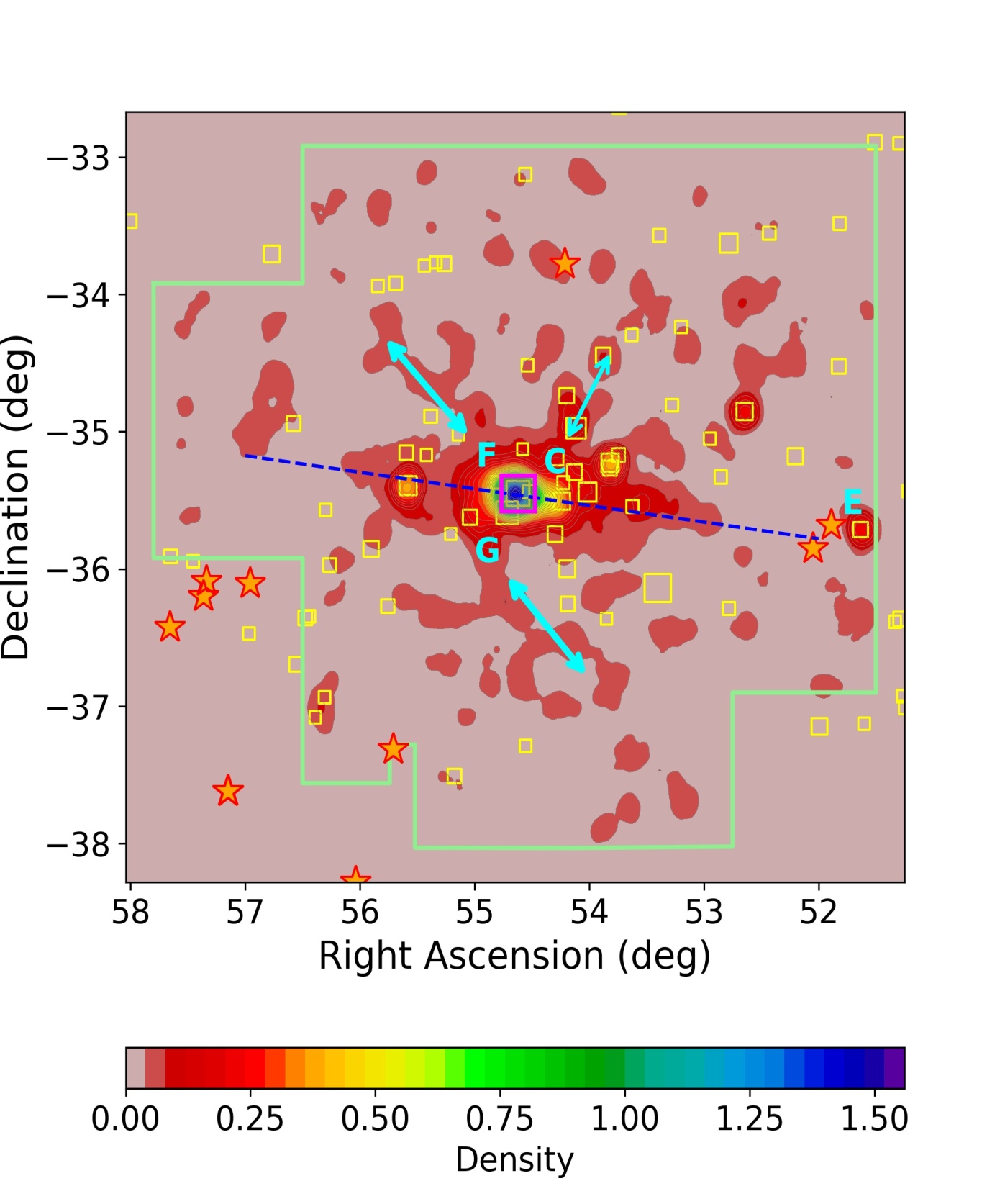
Figure 11: Single panel view of the 2-D GC surface distribution. Iso-density contours and symbols are the same as in Figure 10 (third contour level plots). Light blue arrows and labels indicate the GC overdensities discussed in the text. The blue dashed line shows the $\sim 10^{\circ}$ tilt in the direction of NGC 1336 (’E’ label in the figure).

$\bullet$ Central over-density: For sake of clarity, in Figure 11, we plot the density map relative to the third contour plot (third row in Figure 10). The peanut shaped distribution of GCs, elongated in the E-W direction of the cluster, with a marked peak on NGC 1399, was already found in our studies relying on data of the central FDS area, within $52.5\leq R.A.\leavevmode\nobreak\ (deg)\leq 56.5$ and $-37\leq Dec.\leavevmode\nobreak\ (deg)\leq-35$ (a total of $\sim 7.5$ sq. degrees).

In the new dataset, covering $\sim 4$ times the area previously inspected, we find a $\sim 10$deg tilt of the position angle for the broad distribution of inter-galactic GC candidates, tilting in the direction of NGC 1336 (the tilt direction is also indicated with a blue dashed line in Figure 11). The length of the last isodensity contour is $a=2.6\pm 0.2\leavevmode\nobreak\ deg$ (or $920\pm 60$ kpc), obtained combining the sizes from the four maps in Figure 10. The width of the distribution is of $b=0.89\pm 0.03\leavevmode\nobreak\ deg$ (or $310\pm 10$ kpc), implying an ellipticity $\epsilon=1-b/a\sim 0.65$, slightly larger than what previously found on smaller scales (Kim et al., 2013; Cantiello et al., 2018a).

$\bullet$ $F$ & $G$ features: In the distribution, besides the obvious case of NGC 1399 and its fainter close companions, we observe several regions of marked over-density in correspondence with bright galaxies or pair of galaxies: NGC 1427, NGC 1374/1375, NGC 1351, all with $B_{T}\leq 12$ mag, and of NGC 1336, which is $\sim 1.5$ mag fainter than the others. The GCs peaks on these regions were already commented in our previous works. However, thanks to the larger area analyzed and the different detection strategy the new photometric sample reaches $\sim 1$ mag deeper $u$-band, we now find that such structures are connected and extend to larger clustercentric radii. The $F$ and $G$ features described in D’Abrusco et al. (2016) (arrows in Figure 11) extend $\sim 1.5$ degrees ($\sim 0.5$ Mpc) South-West and North-East of the cluster core, respectively. These substructures do not cross any galaxy brighter than $B_{T}=16$ mag, both overlap a handful of galaxies with $16\leq B_{T}\leq 18$ mag (absolute magnitude $-15.5\leq M_{B,tot}\leavevmode\nobreak\ (mag)\leq-13.5$), and a dozen of fainter galaxies, down to $B_{T}\sim 20$ mag ($M_{B,tot}=-11.5$ mag). The $F$ extension, points toward a group of five galaxies with magnitudes $B_{T}$ between 13.5 and 16 mag, dominated by ESO 358-050, where no GC structure or overdensity is noticeable in any of the GC color-contour selections.

The level of persistence of the $F$ and $G$ structures changes with the selection contours. To estimate the level of significance of both these overdensities we proceed as follows. First, taking as reference the third contour level in Figure 10, we count the number of GC candidates in the $F$ and $G$ feature density contours ($N_{X}$, with $X$ referred to the $F$ or $G$ region). Then, to define a background level, we move the same density contours around the FDS area, avoiding the central overdensity and the regions with galaxies brighter than $B_{T}\sim 16$, and count the number of candidates in such regions. For each feature, we identified seven independent regions for background estimation over the survey area; then we used the median and $rms_{MAD}$ of the GC number counts in the seven regions ($N_{X,back.}$, $rms_{X,back.}$) to quantify the $F$ and $G$ overdensity ratio as follows:
$\Sigma[(in{-}out)/err]=(N_{X}-N_{X,back.})/(rms_{X,back.}^{2}+\delta N_{X}^{2})^{1/2}$.

By definition, $\Sigma[(in{-}out)/err]$ quantifies the ratio between the difference of counts in and out the $X$ feature, and the squared sum of the standard deviation of both counts, assuming a poissonian fluctuation for $N_{X}$ ($\delta N_{X}=N_{X}^{1/2}$). We obtain $\Sigma[(in{-}out)/err]\sim 4.2$, for $F$ and $\sim 4.4$ for $G$, meaning that the GC candidates overdensity with respect to the diffuse background GCs component, is at least factor of four larger than the estimated total expected counts fluctuation in both regions. A similar result, although on smaller regions, with a different (shallower) sources catalog and with independent algorithms, was found by D’Abrusco et al. (2016).

The $F$ is more evident in the wider color-contours selections (upper two panels in Figure 10), which also include the red GCs, that are mostly expected to be closely bound to the galaxies; because of the wider selection intervals, this feature is also likely to have higher fore/back-ground contamination. The $G$ structure, instead, appears more connected to the blue GC population (lowermost panel in the figure); the properties of such coherent structure extending over cluster scale, over an area devoid of bright galaxies and composed mostly of blue GCs –the GC sub-population typically found in the outer galactic regions– suggest its inter-galactic nature. We speculate that the $G$ feature might be connected with NGC 1404, as a stream of blue GCs possibly leading/tailing from the galaxy; the galaxy has an overall $z$-band specific frequency $S_{N,z}=0.30\pm 0.00$, and within one effective radius $S_{N,z,In}=0.12\pm 0.01$ (Liu et al., 2019). The whole median of the ACSFCS sample is $\langle S_{N,z}\rangle=0.82\pm 0.37$, or $0.93\pm 0.26$ if limited to the five brightest galaxies in the main Fornax cluster after excluding NGC 1399 and NGC 1404 itself; for the $S_{N,z,In}$ from the combined Fornax and Virgo cluster sample (Table 4 in Liu et al., 2019), and limited to galaxies brighter than $M_{z}\sim-20.7$ mag, we obtain $\langle S_{N,z,In}\rangle=0.32\pm 0.18$. Hence, in all cases NGC 1404 is a noteworthy case of bright galaxy with a GC population consistently lower than average. Bekki et al. (2003) have a dynamical model for the GCs system of NGC 1404, explaining its low specific frequency as an effect of the tidal stripping of GCs by the gravitational field around cluster core, dominated by NGC 1399. The authors find that, at given models input conditions (highly eccentric orbit, initial scale-length of the GCs system twice as large as the galaxy effective radius) NGC 1404 GCs population can be reduced through stripping to the presently observed value. One of the observable characteristics predicted by Bekki et al. is the formation of an elongated or flattened tidal stream of GCs.

Furthermore, the complex structure of the Fornax X-ray halo (Paolillo et al., 2002; Su et al., 2017) has been explained by Sheardown et al. (2018) using hydrodynamics simulations, by the orbital motion of NGC 1404 within the cluster, assuming that the galaxy is at its second or third passage through the cluster center.

$\bullet$ NGC 1336: The new photometry confirms the peculiarity of NGC 1336 with respect to the rest of the cluster: we find its GCs overdensity ($E$ feature in D’Abrusco et al., 2016) isolated with respect to the rest of the cluster-wide GCs system. The distinctiveness of NGC 1336 is also discussed by Liu et al. (2019), who find that it has the second highest GC specific frequency, after NGC 1399, and the largest 3D clustercentric distance in the ACSFCS sample. The relative isolation of the galaxy from the Fornax core, at $\sim 2$ times of the cluster virial radius, also supported by the lack of GC streams toward the core, might strengthen the hypothesis by Liu et al. that it ”is an infalling central galaxy with a higher total mass-to-light ratio, resembling the behavior of the most massive ETGs. Its GC system has possibly experienced fewer external disruption processes, and the GCs may have a higher survival efficiency.” The presence of two kinematically decoupled cores (Fahrion et al., 2019b), most probably evidencing a major merger that has altered the structure of NGC 1336 significantly, might further support such hypothesis.

$\bullet$ The $C$ feature: A further structure, labeled $C$ in D’Abrusco et al., ranges from NGC 1380 North-West in the direction of the ringed barred spiral NGC 1350. The feature appears less coherently connected than the $F$ and $G$ in the maps of Fig. 10, and it crosses four galaxies with $B_{T}\leq 16$, thus it might be the result of the projected superposition of several adjacent GC systems, rather than an intra-cluster GCs structure.

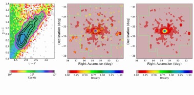
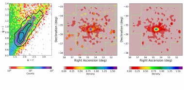
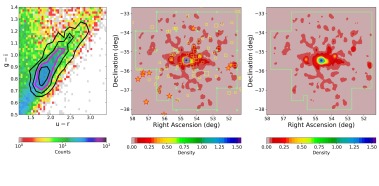
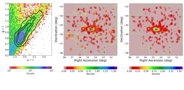
Figure 10: Surface density maps of GC candidates over the FDS area. Upper left panel: Color-Color Hess diagram for GC candidates selected using the parameters in Table 8. The contour lines refer to the master GC sample. All GC candidates in the color-color contour level shown with a thick magenta solid line (also evidenced with a gray shaded area) are used for the density maps in the middle and right panels. Upper middle panel: Density map of the GC candidates within the shaded area highlighted in the left panel. The density is in number of candidates per square arcmin. East is left, north is up. The light green line shows the FDS footprint; filled green dots mark the limits of single pointings; five pointed stars mark stars with $m_{V}\leq 7$ mag; yellow squares show galaxies brighter than $B_{T}=16$ mag, with symbol size scaled to galaxy total magnitude; NGC 1399 is also marked with a magenta empty square. Upper right panel: as upper middle panel, except that all reference sources and lines are not plotted to highlight the GC structures in the area. Second to fourth row of panels: as upper row, but for the other narrower contour levels of the color-color diagram, as evidenced with the magenta contour in the first column of panels. From upper to lower panels the number of GC candidates within the color-color region identified with red contour level is: 5.650, 3.650, 2.170, and 900, respectively.

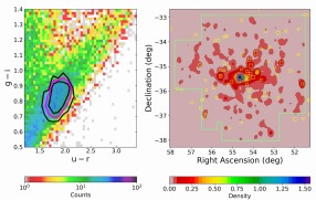
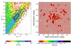
Figure 12: The two-dimensional density maps of blue (upper panels) and red (lower panel) GC candidates. Symbols are the same as in Figure 10.

$\bullet$ Blue and red GCs, foreground stars: We also plot the map of blue and red GC candidates in Figure 12, using the color-contours shown in the left panels. To improve the blue/red GCs separation, taking advantage of the availability of two colors, the separation between red and blue GC is taken from a linear fit to the $(u{-}r)$ -$(g{-}i)$ sequence of the master GC sample, then taking the blue/red separation from the dip in the distribution projected along this axis, a procedure we already used in Angora et al. (2019, see their Figure 7, upper panel). The blue/red surface density maps show the property already anticipated above of red GCs being concentrated on galaxies, especially on bright ellipticals, and blue GCs covering a wider area, including the intra-cluster regions.

For comparison with the previous maps, Figure 13 shows the stellar density map, where stars are identified as the bright sources $16\leq m_{g}\leavevmode\nobreak\ (mag)\leq 20.5$, with the same photo-morphometric properties of GCs (Table 8) except no color selection is applied. The stellar map shows both the lack of any obvious structure over the field, and the large contamination from MW stars: the map, limited to the brightest part of the field MW stellar population, is derived from $\sim 23.000$ stars, versus the $\sim 5.600/900$ GCs used for the GC maps in Figure 10, and the $\sim 2.200/1200$ blue/red GCs selected for the maps in Figure 12.

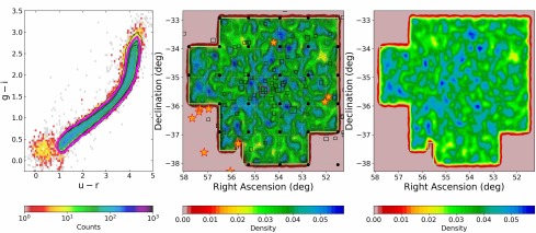
Figure 13: The surface density maps of bright stars. Symbols are the same as in Figure 10.

$\bullet$ UCD galaxies: A further map from the $ugri$ catalog is shown in Figure 14, with the UCD surface density distribution over the FDS area, derived using the selection parameters for UCDs, reported in Table 8, and the color contours of known UCDs from the reference sample (magenta solid lines in the figure). Unsurprisingly the surface density maps show the concentration of UCDs rises around the central square degree area of NGC 1399. The map is mostly shown for completeness, as number of UCDs is known to be small, so even a small contamination can significantly alter the analysis. With our selection we identify 160 sources, which probably include a substantial fraction of contaminating stars, especially in the brightest magnitude bin ($19\leq m_{g}\leq 20$), and bright GCs with morphological parameters consistent with the UCDs. Inspecting separately the maps of bright/faint UCDs candidates, adopting as separation limit $m_{g}=20$ mag, we observe that the map for the faint magnitude bin – $m_{g}=20$-$21$ containing 105 candidates at the given selection criteria – doesn’t change notably with respect to Fig. 14, and shows an elongated density structure with a peak close to the cluster core, and two secondary maxima at [RA, Dec.]=[53.7, -37.6] and [52.3, -33.5]. The map of the bright component – $m_{g}=19$-$20$, 55 candidates – does not show any noteworthy pattern, with sources appearing evenly distributed in the region, a behavior suggesting large contamination from MW stars in this magnitude range. The study of the UCD distribution over the area requires a dedicated analysis to characterize and identify all the selected UCD candidates, which is beyond the scopes of this study, and will be addressed in a forthcoming work, also using near-IR photometry (Saifollahi et al., in prep.).

In conclusion, it is worth highlighting that all the sub-structures described in this section are relatively insensitive to the main parameters chosen to identify GC or UCD candidates, and to the details of the algorithms used to derive the maps themselves, except minor details which leave unaltered the general presentation above.

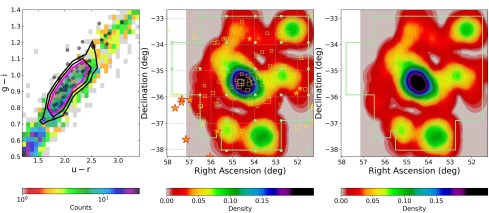
Figure 14: The surface density maps of UCD candidates. Symbols are the same as in Figure 10.

3.2.2 GCs distribution maps over the FDSex area

The lack of $u$-band photometry over the FDSex area implies that any sample of compact sources selected in the area using the same procedures adopted in the previous section, yet based only on $gri$ photometry, is more contaminated. In Figure 15 we plot the contour levels of the master GC sample (blue lines and shaded area), and the contour levels of compact (green color, $C.I_{n}\sim 1$) and extended (red colors, $CI_{n}\geq 1.3$) sources, all brighter than $m_{g}=22.5$ mag, using the $ugri$ catalog. The bright magnitude cut is adopted to reduce the scatter due to increased photometric errors at fainter magnitudes. The diagrams show that the sequence of GCs/UCDs/stars in the $(g{-}i)$ -$(g{-}r)$ matches with the sequence of extended objects, while in the $(g{-}i)$ -$(u{-}r)$ diagram the degeneracy is less dramatic, making more efficient the separation of compact/extended sources.

To obtain a rough estimate of the increase of contamination due to the lack of $u$-band photometry we proceed as follows. Using the $ugri$ catalog in the FDS area, we adopt the GC selection scheme described in the previous section but use the $(g{-}i)$ -$(g{-}r)$ color combination, instead of the $(g{-}i)$ -$(u{-}r)$ , for the selections on the color-color plane. y comparing the number of GC candidates identified using the $(g{-}i)$ -$(u{-}r)$ color-color, $N_{ugri}^{GC}$, with the number of candidates identified using $(g{-}i)$ -$(g{-}r)$ color-color, $N_{gri}^{GC}$, we find $(N_{gri}^{GC}-N_{ugri}^{GC})/N_{gri}^{GC}\sim 0.48$. Therefore, this single change in the criteria for GC selections implies the number of sources identified as GC candidates is nearly doubled over the FDS area. Such increase is not spatially uniform: it is close to $\sim 80\%$ in background regions, i.e. far from bright galaxies and their host GC system, and drops to $\sim 15\%$ around bright galaxies. This difference shows that GC selection in the central cluster area, where GCs have a high surface density, is already quite efficient with a 3-band combination. In contrast, the addition of the $u$-band makes a significant difference in GC selection in the outer parts of the cluster where the fractional background contamination, mostly due to MW stars, is higher.

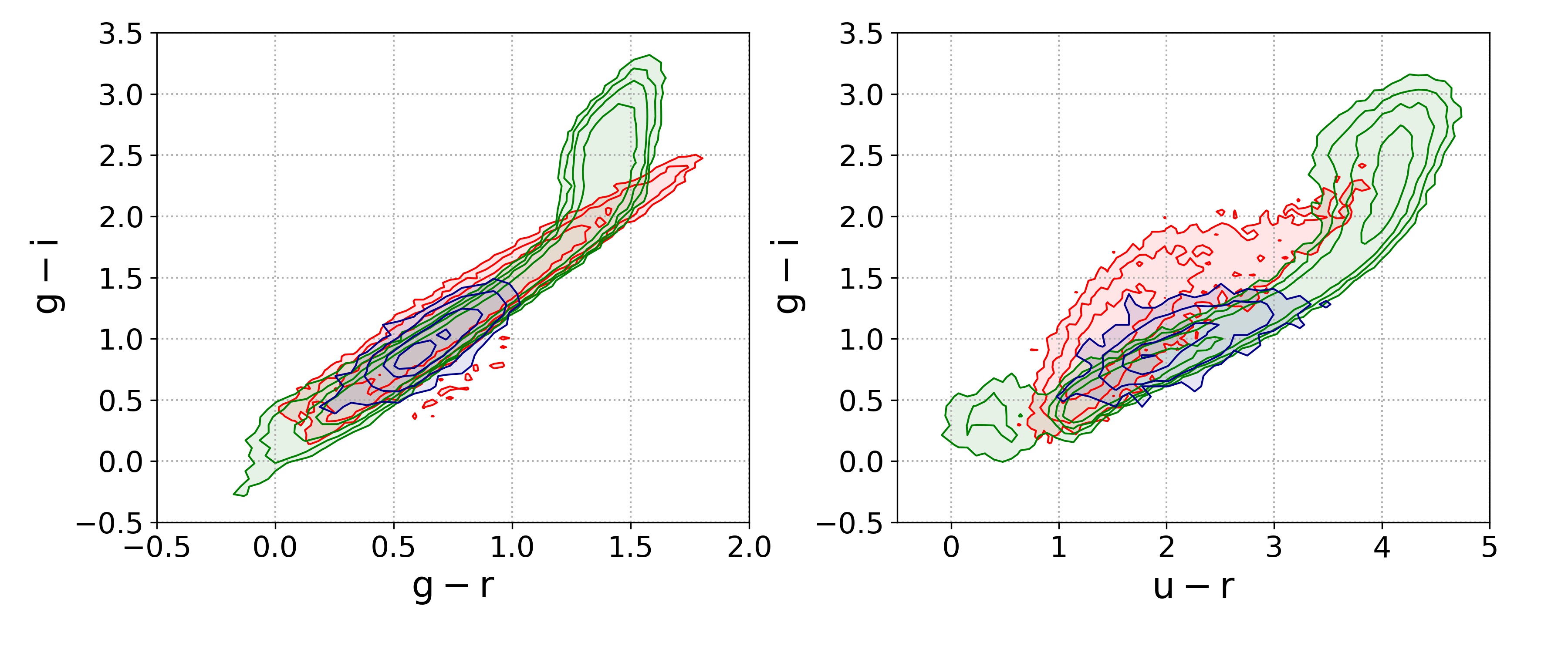
Figure 15: Color-color contour plots of the GC master catalog (blue contours and shaded area), of point-like sources (green) and of extended sources (red).

In spite of the higher level of contamination, the FDSex $gri$-band catalog also includes the area of NGC 1316, Fornax A, the brightest galaxy in the cluster in optical bands, a peculiar giant elliptical, suggested being in its second stage of mass assembly (Iodice et al., 2017b). It is then of particular interest to show here, for the first time, the global properties of the GCs over such wide area. We should, however, be aware that NGC 1316 is known to contain relatively young GCs ($\sim 2-3$ Gyr, e.g. Gómez et al., 2001; Goudfrooij et al., 2001; Sesto et al., 2017), which are not part of our reference sample. Young GCs are in general bluer and brighter than equally massive old GCs; hence, we bear in mind that our selection is intrinsically biased toward old GCs.

Using the same procedures described in the previous sections, except that $(g{-}r)$ is used instead of $(u{-}r)$ , we analyze the surface distribution maps over the 27 sq. degrees of the FDSex area. For sake of clarity in Figure 16 we only show the second color-color density contour, corresponding to the iso-density contour level of 15 GCs from the master catalog. In the panels of the figure, no obvious GC substructure appears bridging the core of the main Fornax cluster to the Fornax A sub-group. The two brightest galaxies, NGC 1399 and NGC 1316, are $\sim 3.6\deg$ apart ($\sim 1.3$ Mpc) and the density map of the $\sim 10.200$ GCs selected does not reveal any hint of residual GC tails along the direction connecting the bright ellipticals, with the possible only exception of the East-West elongation of GCs around the cluster core still visible in the $gri$ map, although with less details compared with the $ugri$ maps.

The higher level of contamination of the $gri$ maps appears in some spurious features. Figure 16 shows a structure around the area of coordinates [R.A.=52 deg, Dec.=-34 deg], characterized by nearly the same geometric appearance of the FDS fields #14, #19 and #31. Such structure is completely unseen in the $ugri$ maps which also cover the area; inspecting the three FDS fields we find slightly deeper limiting magnitudes and slightly poorer source compactness relative to the neighboring fields: combined, two effects generate larger number of detections with poorer morphologic characterization, hence a higher fraction of GCs contamination.

To have a less contaminated sample, we narrowed the sample of GC candidates by using a brighter magnitude cut, more stringent ranges on the various morphological parameters in Table 8, and narrower color-color regions. Using narrower selections, the spurious structure around the fields FDS#14/19/31 disappears. Nevertheless, no matter how much the GC sample is narrowed with more strict selections, no GC substructure emerges along the NGC 1316/NGC 1399 direction.

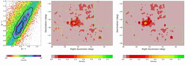
Figure 16: Same as in Figure 10, except that over the FDSex area, and the $(g{-}i)$ -$(g{-}r)$ color-color diagram is used for GCs selection. The position of NGC 1316 is shown with light-blue empty triangle in the middle panel.

By counting the number of GCs candidates within a given radius centered on each of the two bright galaxies within the respective environments, we find that the number of GCs around NGC 1399 outnumbers NGC 1316 by a factor of 4-4.7 at galactocentric radii $R_{gal}$ of $\sim 6\arcmin$ and $\sim 24\arcmin$, and by a factor of $\sim 3$ out to $R_{gal}\sim 40\arcmin$. Figure 17 shows the number ratio $N_{ratio}^{Sources}(\leq R_{gal})=N^{Sources}_{N1399}/N^{Sources}_{N1316}$ versus galactocentric distance for GCs candidates (black line in the figure), for galaxies brighter than a given limit (as labeled in the figure), and the flux ratio of the $r$-band integrated magnitudes of the two galaxies (from Iodice et al., 2016, 2017b, light-blue line in the figure).

The median $N_{ratio}^{galaxies}$ for galaxies in the range of $6\arcmin-24\arcmin$ is $\sim 2.0$ with $rms_{MAD}=0.3$. Assuming a nearly uniform contamination of the FDSex catalogs around the two regions, we estimate the overdensity of GCs around NGC 1399 compared to NGC 1316 ($N_{ratio}^{GCs}\sim 4$) is a factor of $\sim 2$ larger than the overdensity of galaxies in the magnitude range $11.5\leq B_{T}\leavevmode\nobreak\ (mag)\leq 16.5$ ($-20\leq M_{B,tot}\leavevmode\nobreak\ (mag)\leq-15$). Hence, even accounting for the larger density of bright and faint galaxies of all morphological types, the population of GCs is considerably larger in the region of $6\arcmin\leq R_{gal}\leq 24\arcmin$ around NGC 1399 compared with NGC 1316, and mainly composed of blue GCs.

This overpopulation of GCs is likely associated with the intra-cluster GCs component; on the contrary, the relative GCs under-density around Fornax A, and the lack of any major accretion events of NGC 1316 that could have significantly increased the specific frequency of blue GCs, is possibly at the basis of the lack of any significant GC substructure. Furthermore, as expected from the known factor of $\sim 2$ higher total magnitude of NGC 1316 compared to NGC 1399, the $r$-band flux ratio between the two ellipticals is $\sim 0.4\pm 0.1$ (light–blue line in Figure 17), a factor of $8-10$ lower than the GCs count ratio.

Figure 17 also shows some other features : $a)$ the GCs and bright galaxies with $B_{T}\leq 11.5$ mag and $B_{T}\leq 13.5$ mag ($M_{B,tot}=-20$ and $-18\leavevmode\nobreak\ mag$, respectively) have $N_{ratio}^{galaxy}\sim 3$ at $R_{gal}\geq 30\arcmin$, while for the fainter galaxy bin limits we find $N_{ratio}^{galaxy}\sim 1.3$; $b)$ the nearly flat GCs $N_{ratio}$ within $9\leq R_{gal}\leavevmode\nobreak\ (\arcmin)\leq 20$, which assumes a value of $4.66\pm 0.04$. A more detailed analysis of such properties combined with the data in other galaxy clusters is in progress (Cantiello et al., 2020, in prep.)

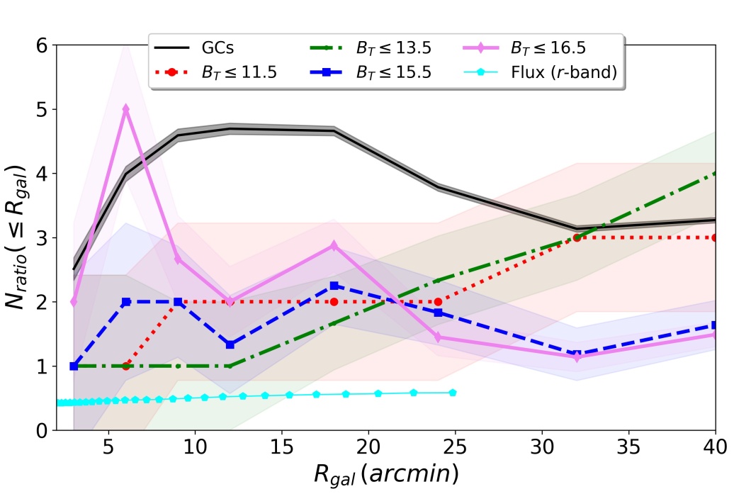
Figure 17: Number ratio of the total number of sources around NGC 1399 and NGC 1316 within a given galactocentric radius in the respective environment: $N_{ratio}(\leq R_{gal})=N_{Sources}^{N1399}/N_{Sources}^{N1316}$. The number ratio for GCs is shown with a black solid line; number ratios for galaxies at a given bright magnitude cut are also shown, and labeled. The $r$-band flux ratio between the two galaxies within $R_{gal}$ is shown with light-blue solid line and pentagons.

4 FDS catalogs of background sources and related science

The depth and spatial resolution of the FDS images, together with ancillary data from other spectral ranges available in this field, provide the opportunity to study the stellar populations and structural properties of galaxies beyond the cluster, as well as to discover rare astrophysical objects, like compact massive galaxies and strong gravitational lenses (e.g., Tortora et al. 2018; Petrillo et al. 2017). The FDS image quality is similar to the one of the KiDS survey (Kuijken et al., 2019), since the longer exposures in FDS images are balanced by a slightly poorer seeing ($r$-band FWHM of $\sim 0\aas@@fstack{\prime\prime}9$ for FDS, vs $\sim 0\aas@@fstack{\prime\prime}65$ in KiDS). The limiting magnitudes in the two surveys are quite similar, but FDS is deeper in $i$-band.

Taking advantage of the FDS data, we aim at determining photometric redshifts, stellar masses, galaxy classifications and structural parameters of thousands of background galaxies. This will provide a complete characterization of the background galaxy population over the area, for investigating the evolution of the structural and stellar properties of galaxies as a function of redshift and mass. The tools for deriving all required quantities are already available and well tested in our team (e.g. La Barbera et al., 2008; Cavuoti et al., 2017; Roy et al., 2018).

As a first test on the background galaxy population in FDS, we run a code to find galaxy-galaxy lens candidates. The code uses a machine learning classification method based on Convolutional Neural Networks (CNNs), and was already applied to the KiDS survey (de Jong et al. 2017; Petrillo et al. 2019). We performed the run of CNN with a network trained on a large sample of $r$-band (or combined $g$-$r$-$i$) KiDS images, to the equivalent FDS images. Although the network is not customized and trained on FDS images, KiDS and FDS are based on data from the same telescope and camera, and, as mentioned above, are comparable in both FWHM and depth. Therefore, this is a valid approach to search gravitational lenses in FDS. In fact we already discovered several gravitational lens candidates in the FDS fields, two of them, with FDS catalogue ID and coordinates: FDSJ032720.32-365821.81 at [51.834682; -36.972725] and FDSJ034739.60-352516.23 at [56.91502, -35.421176], are presented in Figure 18 as an example of the potential of this approach.

Figure 18: Two example lens candidates found in the FDS fields applying the CNN code; the image cutout have $20\aas@@fstack{\prime\prime}0$ side. Left: FDSJ032720.32-365821.81, right: FDSJ034739.60-352516.23

5 Conclusions

We have presented the photometric and morphometric catalog of compact and slightly extended sources in the Fornax galaxy cluster, derived with VST observations within the FDS survey over an area of $\sim 21$ square degrees in $ugri$-bands, and in $gri$-bands for a total of $\sim 27$ square degrees.

The $ugri$ data of FDS cover the main body of Fornax, centered on NGC 1399, and extend out to $\sim 1\leavevmode\nobreak\ Mpc$, the virial radius of the cluster. The $gri$ coverage, FDSex, extends to the South-West region of the Fornax A sub-cluster with its brightest galaxy, NGC 1316.

Because of the large FWHM variation from field to field, to improve the uniformity of sources detection and their morphological characterization, we derived a master-detection frame by coadding all $gri$ single exposures with $FWHM\leq 0\aas@@fstack{\prime\prime}9$; starting from a median FWHM ranging from $0\aas@@fstack{\prime\prime}92$ to $1\aas@@fstack{\prime\prime}26$ with $rms$ within $0\aas@@fstack{\prime\prime}11-0\aas@@fstack{\prime\prime}17$ for the various bands, adopting the multi-band stacking procedure we ended up with a master-detection frame with a median FWHM of $0\aas@@fstack{\prime\prime}80\pm 0\aas@@fstack{\prime\prime}04$, $\sim 15\%$ improvement over the median FWHM of the highest resolution imaging ($r$-band), and a factor of $\sim 2.5$ lower $rms$.

We calibrated the photometry using a two-step procedure, to reduce the effect of the independent calibration of the FDS fields, which generate a non-negligible photometric offset between neighboring fields. The first calibration step follows the standard calibration plan of VST frames. As a second step, we used the APASS photometry to derive a matrix to match the full FDS catalog to a unique reference. With this approach, the photometric offset between fields becomes negligible, and the re-calibrated photometry shows a general good match to existing literature data from SKyMapper, from the HST/ACSFCS survey and to predictions from stellar population synthesis models.

The catalogs are available through the project web pages, and will also be available on CDS. In the catalogs we provide the position, the photometry and the morphometry for 1.7 million sources with $ugri$ detections, and for 3.1 million sources with $gri$ data.

As a preliminary use of the catalogs, we analysed the 2-D distribution of compact stellar systems in the area, with particular care to GCs.

With the FDS instrumental setup, and at the distance of Fornax, GCs are by all means point-like sources, except for a possible fraction of $\ \raise-2.0pt\hbox{\hbox to0.0pt{\hbox{$\sim$}\hss}\raise 5.0pt\hbox{$<$}\ }0.5\%$ of the population. Hence, GCs can be identified by their compactness.

To obtain the least contaminated GCs sample, we selected a number of morpho-photometric features, and analysed them over a reference catalog of confirmed GCs and UCDs in Fornax. Such catalog is build by cross-matching the FDS catalogs with available spectroscopic and photometric datasets of confirmed GC/UCD. The reference catalog is then used to define the GCs loci in the parameter space, for the chosen photometric and morphometric parameters.

The GCs maps over the FDS area confirm the results of previous studies, about the presence of a large inter-galactic GC population around the main body of the cluster, centered on NGC 1399, stretched along the East-West direction. Here we find a small tilt of the distribution in the direction of NGC 1336 by $\sim 10\deg$. The distribution appears to extend over $\sim 1\leavevmode\nobreak\ Mpc$ from side to side, highly flattened, with an ellipticity of $\sim 0.65$. In addition to our previous results, we find that one of the features already discussed, which extends from the main cluster body to the South-West direction, might be a tail of relatively blue GCs from NGC 1404, a bright galaxy close to the cluster core and with a peculiarly poor GCs population.

Of the GCs features already commented in the past, we here highlight the case of NGC 1336, which we confirm to be relatively isolated from the cluster, and with a high specific frequency of GCs; this might support the hypothesis that it is an infalling massive galaxy, with a GCs system that possibly experienced only few disruption processes. We also inspected the blue/red GCs maps, and confirm the known property of blue GCs residing in the wider cluster area, and red GCs being more concentrated on massive galaxies.

Systems selected to fit the color-magnitude range of spectroscopically confirmed UCDs show a substantial overdensity in the central cluster. The 160 UCD candidates are about three times more than the currently known UCDs in Fornax and would require spectroscopic follow up to learn more about their nature.

We also derived the GCs maps over the FDSex area, which has the disadvantage of suffering for larger contamination because of the lack of $u$-band over the NGC 1316 area, but has the advantage of covering this brightest cluster galaxy. With the caveat that the $gri$ catalogs do not allow the detailed analysis allowed over the FDS area, despite our attempts to obtain a cleaner GC candidates sample, we do not find significative GCs structures along the NGC 1399-NGC 1316 direction, which extends over a projected distance of $\sim 1.3\leavevmode\nobreak\ Mpc$. This might be due to the lower efficiency of the GC identification. However, assuming similar contamination of the $gri$ catalogs over the NGC 1399 and NGC 1316, we find that the GC population of the former outnumbers the second by a factor of $\sim 4$, and by about a factor of $\sim 10$ when normalized to galaxy luminosity, within a galactocentric range of $6\arcmin-24\arcmin$, and remains a factor of $\sim 3$ higher than NGC 1316 at larger galactocentric radii, out to $\sim 40\arcmin$. Hence, the ’contrast’ of the GC populations towards NGC 1316 might be too low for the purpose of our study, – in spite of its luminosity twice larger than NGC 1399 – and might explain the difficulty in finding GCs sub-structures, which intrinsically need a large number of candidates over a given region to be identified. The rich intra-cluster GCs population around NGC 1399 does not seem to be matched by a similarly rich system around NGC 1316, the brightest galaxy of the Fornax A sub-cluster. In spite of this, the lack of obvious GC sub-structures between these two bright and massive galaxies might also be consequence of the NGC 1316 sub-cluster being in its first infalling phase and evolving autonomously, a result also supported by an independent analysis of FDS data for galaxy surface brightness profiles and intracluster light (Iodice et al., 2017b; Raj et al., 2019).

A deeper analysis of the 2-D maps, and other characteristics of the GCs over the FDS and FDSex area is in progress, and will be presented in a dedicated paper.

We finally presented an example use of the catalogs to analyze background galaxies. Using machine learning methods, already tested on the KiDS survey with VST, we identified two lens candidates in the FDS area.