ATOMS: ALMA Three-millimeter Observations of Massive Star-forming regions – II. Compact objects in ACA observations and star formation scaling relations

Abstract

We report studies of the relationships between the total bolometric luminosity ($L_{\rm bol}$ or $L_{\rm TIR}$) and the molecular line luminosities of $J=1-0$ transitions of H¹³CN, H¹³CO⁺, HCN, and HCO⁺ with data obtained from ACA observations in the "ATOMS" survey of 146 active Galactic star forming regions. The correlations between $L_{\rm bol}$ and molecular line luminosities $L^{\prime}_{\rm mol}$ of the four transitions all appear to be approximately linear. Line emission of isotopologues shows as large scatters in $L_{\rm bol}$-$L^{\prime}_{\rm mol}$ relations as their main line emission. The log($L_{\rm bol}$/$L^{\prime}_{\rm mol}$) for different molecular line tracers have similar distributions. The $L_{\rm bol}$-to-$L^{\prime}_{\rm mol}$ ratios do not change with galactocentric distances ($R_{\rm GC}$) and clump masses ($M_{\rm clump}$). The molecular line luminosity ratios (HCN-to-HCO⁺, H¹³CN-to-H¹³CO⁺, HCN-to-H¹³CN and HCO⁺-to-H¹³CO⁺) all appear constant against $L_{\rm bol}$, dust temperature ($T_{\rm d}$), $M_{\rm clump}$ and $R_{\rm GC}$. Our studies suggest that both the main lines and isotopologue lines are good tracers of the total masses of dense gas in Galactic molecular clumps. The large optical depths of main lines do not affect the interpretation of the slopes in star formation relations. We find that the mean star formation efficiency (SFE) of massive Galactic clumps in the "ATOMS" survey is reasonably consistent with other measures of the SFE for dense gas, even those using very different tracers or examining very different spatial scales.

1 Introduction

Since the pioneering works by Gao & Solomon (2004) and Wu et al. (2005), many observational studies toward external galaxies (Graciá-Carpio et al., 2006; Juneau et al., 2009; García-Burillo et al., 2012; Greve, 2014; Zhang et al., 2014; Liu et al., 2015; Chen et al., 2015; Tan et al., 2018; Jiménez-Donaire et al., 2019) and Galactic molecular clouds (Wu et al., 2010; Liu et al., 2016; Stephens et al., 2016) have revealed a strong linear relationship between the recent star formation rate (SFR), as traced by the total infrared emission, and the dense molecular gas mass that is indicated by line luminosities ($L^{\prime}_{\rm mol}$) of dense molecular gas tracers (e.g., HCN, HCO⁺, and CS). This so called "dense gas star formation law" may imply that the dense molecular gas rather than the total molecular gas is the direct fuel for star formation (Kennicutt & Evans, 2012; Vutisalchavakul et al., 2016). While significant progress has been made in recent years, the origin of this relationship is still under debate.

The $J=1-0$ transitions of HCN and HCO⁺ are among the most commonly used tracers in the studies of "dense gas star formation law". However, the emission lines of these two dense gas tracers tend to be optically thick in dense parts of molecular clouds (e.g., Sanhueza et al., 2012; Hoq et al., 2013; Shimajiri et al., 2017). In the limit that all transitions are optically thin and only collisional excitation is important, but densities are far below the critical density, the emission would be proportional to $n\times n_{\rm mol}$, where $n$ is the number density of colliders (mainly H₂) and $n_{\rm mol}$ is the density of the line-emitting molecules, thus proportional to $n^{2}$ for constant abundance. At the other extreme, the emission from an optically thick, thermalized line (e.g. ¹²CO) is not sensitive to density at all. While the extremes rarely apply, and the rich energy level structure of molecules permits more interesting excitation (masers, cooling of excitation temperatures below the temperature of the CMB, etc.), the above limiting cases illustrate why the emission from rare isotopologues is more highly weighted toward denser regions than their corresponding main lines. To capture some of the effects, the concept of effective excitation density was introduced to indicate the density needed to produce a line of a characteristic strength (1 K km s^-1), given a column density typical for each species (Evans, 1999; Shirley, 2015). The low effective excitation densities of the two main transitions of HCN and HCO⁺ (4.5$\times 10^{3}$ cm^-3 for the HCN $J=1-0$ line and 5.3$\times 10^{2}$ cm^-3 for the HCO⁺ $J=1-0$ line at 20 K; Shirley, 2015) indicate that they can be excited in low density ($n<10^{3}$ cm^-3) gas and are often optically thick.

Indeed, recent observations of nearby Giant molecular clouds (Kauffmann et al., 2017; Pety et al., 2017; Shimajiri et al., 2017) indicate that HCN (1-0) and HCO⁺ (1-0) are easily detected in extended translucent regions at a typical density of 500 cm^-3 and are poor tracers of dense structures such as filaments or cores. Stephens et al. (2016) have argued that most of the Galaxy’s luminosity of HCN may arise from distributed, sub-thermal emission rather than from dense gas. Most recently, Evans et al. (2020) also found that a substantial fraction (in most cases, the majority) of the total HCN (1-0) and HCO⁺ (1-0) line luminosity in six distant ($d\sim$3.5-10.4 kpc) clouds arises in gas below the $A_{\rm V}\sim$8 mag threshold, above which the vast majority of dense cores and YSOs are found in nearby clouds (Heiderman et al., 2010; Lada et al., 2010, 2012). These studies have challenged the ideas that these commonly used tracers (e.g., $J=1-0$ of HCN and HCO⁺) can reveal well the spatial distribution of star forming gas in clouds.

As discussed above, in contrast to the main lines, emission from the isotopologues are optically thinner because of their much lower abundances. The effective densities of H¹³CN $J=1-0$ and H¹³CO⁺ $J=1-0$ at 20 K are about 1.6$\times 10^{5}$ cm^-3 and 2.2$\times 10^{4}$ cm^-3, respectively, which are about 40 times higher than their main lines (Shirley, 2015). Therefore, they can potentially be better tracers of the column densities and dense structures in molecular clouds (e.g., Pety et al., 2017; Shimajiri et al., 2017). The observations of these isotopologues can also help estimate the opacity of their corresponding main line transitions, enabling us to quantify how opacity affects the "dense gas star formation law" with main lines. Studies of the "dense gas star formation law” with isotopologues, however, are very rare. Stephens et al. (2016) used H¹³CO⁺ $J=1-0$ in their studies but they detected the H¹³CO⁺ $J=1-0$ emission only in dozens of sources in their sample of $\sim$300 clumps. In addition, most stars form in gravitationally bound structures (clumps or cores) in molecular clouds. Therefore, it is also essential to evaluate how those lines (main lines and their isotopologues) trace the total gas mass of these gravitationally bound structures.

In this work, we investigate the "dense gas star formation law" with H¹³CN $J=1-0$ and H¹³CO⁺ $J=1-0$ lines as well as their corresponding main lines toward a large sample of 146 Galactic star forming clumps. By doing this, we evaluate the reliability of the main lines being used to trace the total dense gas mass.

This study is part of an ALMA survey program, the "ATOMS" (ALMA Three-millimeter Observations of Massive Star-forming regions). The sample and observations of the "ATOMS" survey are introduced in Liu et al. (2020). The "ATOMS" observed a large sample of 146 active star forming regions with IRAS colors characteristic of UC Hii regions (Bronfman et al., 1996). More than 90% of the sources in the "ATOMS" sample are potentially forming high-mass stars (Liu et al., 2020). In this paper, we only use the data from observations with the Atacama Compact 7 m Array (ACA; Morita Array). The ACA data are particularly useful for this study because they respond primarily to the scale of clumps ($\ga$0.2 pc), rather than cores ($\la$0.1 pc). The dense gas star formation relations will surely break down at the level of cores, but will plausibly be relevant on the scale of clumps.

2 Observations

The ALMA observations of the “ATOMS" survey have been summarized in Liu et al. (2020). We here briefly introduce the observations with the ACA. Observations with the ACA were conducted from late September to mid November in 2019 with band 3 (Project ID: 2019.1.00685.S; PI: Tie Liu). The IRAS names, phase centers (columns 2-3), systemic velocities (column 4), distances (column 5), and galactocentric distances (column 6) of the targeted sources are listed in Table 5. The typical ACA observing time per source is $\sim$ 8 minutes. The angular resolution and maximum recovered angular scale (MRS) in ACA observations are $\sim 13.1\arcsec-13.8\arcsec$ and $\sim 53.8\arcsec-76.2\arcsec$, respectively. The ACA observations are sensitive to angular scales smaller than $\sim 60\arcsec$ but the MRS is larger than the angular sizes of most clumps in the sample (Faúndez et al., 2004). The $J=1-0$ transitions of HCN, HCO⁺, H¹³CN and H¹³CO⁺ are included in four spectral windows in the lower side-band. The spectral resolution for HCN $J=1-0$ and HCO⁺ $J=1-0$ is 61.035 kHz (or $\sim$0.2 km s^-1), while the spectral resolution for H¹³CN $J=1-0$ and H¹³CO⁺ $J=1-0$ is 0.122 MHz (or $\sim$0.4 km s^-1). Calibration and imaging were carried out using the CASA software package version 5.6 (McMullin et al., 2007). The continuum visibility data are constructed using the line-free spectral channels. All images are primary beam corrected. The achieved sensitivity of the ACA observations is around 50-90 mJy beam^-1 per 0.122 MHz channel for lines.

3 Results

3.1 Compact objects

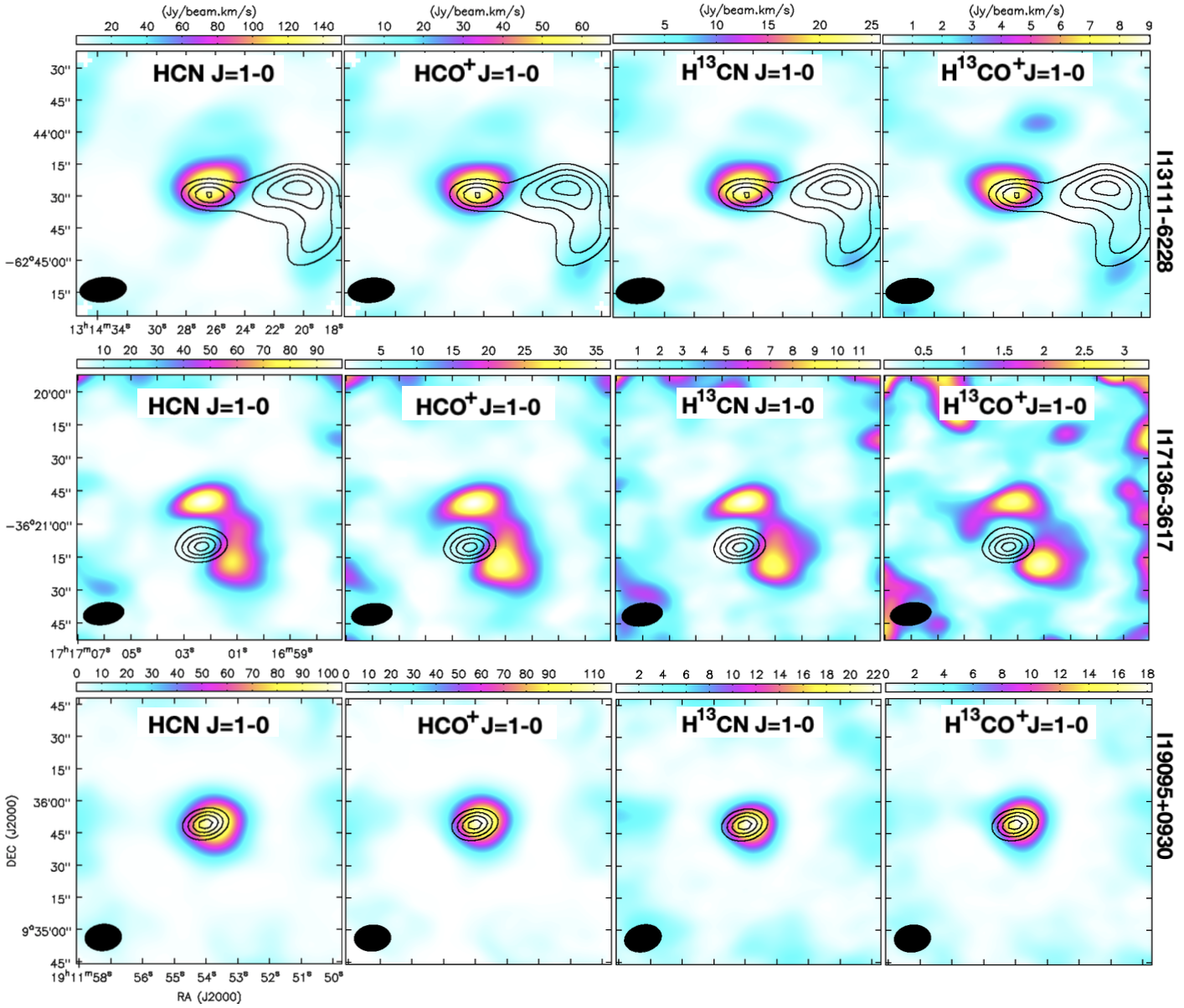
Figure 1: Integrated intensity maps of four molecular lines are shown as color-scale images for three example sources. I13111-6228, I17136-3617 and I19095+0930 are shown in upper, middle and lower panels, respectively. The 3 mm continuum is shown in contours. The contour levels are from 30% to 90% in steps of 20% of peak values. The peak values of 3 mm continuum emission for I13111-6228, I17136-3617 and I19095+0930 are 0.088, 1.814 and 0.307 Jy beam^-1, respectively.

We extracted compact objects from 3 mm continuum emission maps and the integrated intensity maps of the four molecular lines. Figure 1 shows the 3 mm continuum emission and integrated intensity maps for three sources. The compact objects in 3 mm continuum emission and molecular line emission can be easily identified by eye. In total, we detected 173, 184, 190, 189 and 182 compact sources from 3 mm continuum emission, H¹³CN, H¹³CO⁺, HCN, and HCO⁺ line emission, respectively.

As shown in Figure 1 for I13111-6228, we identified multiple compact objects in 3 mm continuum in 27 targets. Some targeted sources also contain multiple objects in molecular line emission as shown in Figure 1 for I17136-3617. We identified multiple objects in 30, 32, 35 and 27 sources from H¹³CN, H¹³CO⁺, HCN, and HCO⁺ integrated intensity maps, respectively. However, the majority ($\sim$80%) of sources contain only a single compact object in 3 mm continuum emission and in molecular line emission as I19095+0930 in Figure 1.

From 2D gaussian fits, we derived the relative coordinates (or offsets), aspect ratio values, effective radii ($R_{\rm eff}$), offsets from brightest continuum emission peaks ($d_{\rm peak}$), peak integrated intensity ($S_{\rm peak}$) and total integrated intensity ($S_{\rm total}$) for each compact object. The aspect ratio value is defined as the ratio between de-convolved FWHM major dimension ($a$) and minor dimension ($b$), and $R_{\rm eff}$ is defined as $R_{\rm eff}=\sqrt{ab}$. For compact objects identified in H¹³CO⁺ $J=1-0$ and HCO⁺ $J=1-0$ line emission, we also derived the source-averaged velocity ($V_{\rm lsr}$) and velocity dispersion ($\sigma$) from their corresponding Moment 1 and Moment 2 maps. All of these parameters are summarized in Tables 5 to 9.

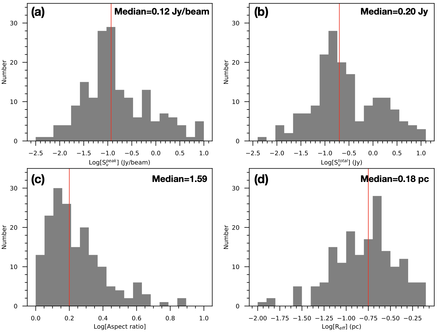
Figure 2: Histograms of parameters for the compact objects identified in 3 mm continuum emission. (a) peak flux density; (b) total flux density; (c) aspect ratios; (d) effective radii. The red solid lines are median values.

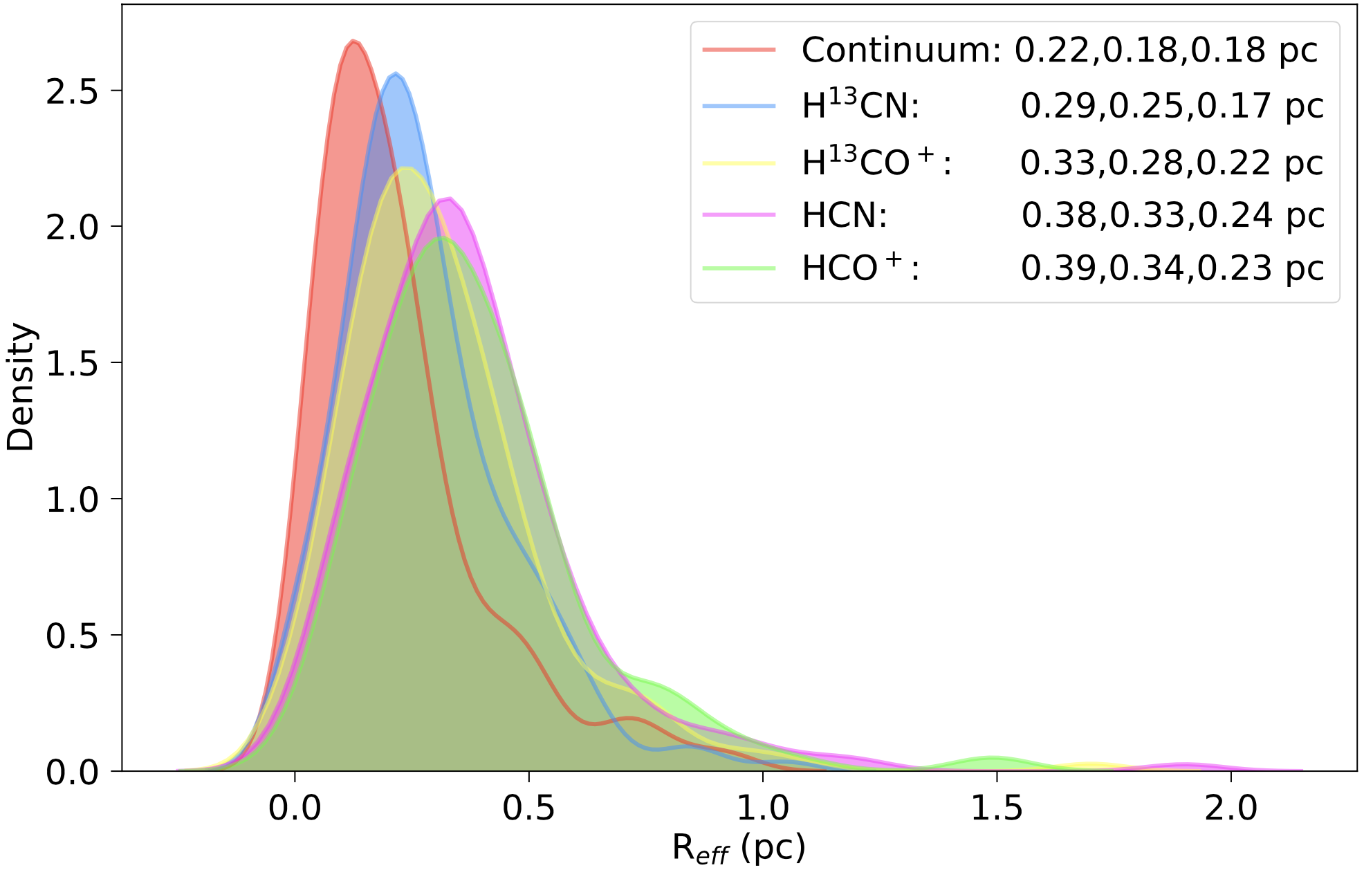
Figure 3: Distribution of $R_{\rm eff}$ for compact objects identified in 3 mm continuum emission and molecular line emission, which are plotted using the function "kdeplot" in the python package Seaborn. The numbers in the upper-right box are mean, median, standard deviation values.

Figure 2 presents histograms of parameters ($S_{\rm peak}$, $S_{\rm total}$, aspect ratio and $R_{\rm eff}$) for compact sources in 3 mm continuum emission. The median values for $S_{\rm peak}$ and $S_{\rm total}$ are 0.12 Jy beam^-1 and 0.20 Jy, respectively. The median value of the aspect ratio is $\sim$1.6. Among the 173 compact objects identified in 3 mm continuum emission, only 18 are with aspect ratio larger than 3. The $R_{\rm eff}$ ranges from 0.01 pc to 0.94 pc with a median value of 0.18 pc. There are 45 compact objects that would be classified as dense cores with $R_{\rm eff}$ smaller than 0.1 pc. There are 14 compact objects in distant sources having $R_{\rm eff}$ larger than 0.5 pc. The detailed properties of those continuum objects will be discussed in forthcoming papers. The 3-mm continuum emission can have a significant contribution from free-free emission, compromising our ability to determine masses from the dust continuum emission. We use instead the literature values for the size (R_eff), mass (M_clump), etc. of the clumps (see Table 10). These are taken from single-dish maps at 0.87 mm (Urquhart et al., 2018) or 1.2 mm (Faúndez et al., 2004), minimizing the contamination by free-free emission.

In Figure 3, we compare the distributions of $R_{\rm eff}$ for compact objects identified in 3 mm continuum emission and molecular line emission. The data are plotted with a gaussian kernel density estimate using the function "kdeplot" in the python package Seaborn. The median radii for compact objects in 3 mm continuum, H¹³CN, H¹³CO⁺ HCN and HCO⁺ line emission are 0.18, 0.25, 0.28, 0.33 and 0.34 pc, respectively. Compact objects in 3 mm continuum emission have statistically smaller $R_{\rm eff}$ than that of compact objects identified in molecular line emission. $R_{\rm eff}$ for compact objects identified in H¹³CN and H¹³CO⁺ line emission are also statistically smaller than compact objects identified in HCN and HCO⁺ line emission. Interestingly, there seems to be a trend between $R_{\rm eff}$ and effective excitation density for the lines. The higher the effective excitation density, the smaller the $R_{\rm eff}$. These results are consistent with the idea that lines with higher effective excitation density trace denser and more compact regions of molecular clouds.

In Figure 4a, we compare the effective radii ($R_{\rm ACA}$) of compact sources in ACA 3 mm continuum emission with the effective radii ($R_{\rm SD}$) of their natal clumps derived in single dish observations. $R_{\rm ACA}$ is linearly correlated with $R_{\rm SD}$ as expected. Since the ACA is resolving out the more extended emission, $R_{\rm ACA}$ is systematically smaller than $R_{\rm SD}$. As shown in Figure 4b, the velocities derived from H¹³CO⁺ $J=1-0$ line emission for compact sources are very consistent with the systemic velocities of their natal clumps from single dish CS J=2-1 line observations (Bronfman et al., 1996).

In some sources such as I17136-3617 shown in Figure 1, gas emission peaks are clearly offset from 3 mm continuum emission peaks by one beam size. These sources may be highly evolved Hii regions that have dispersed their natal gas clumps. In further analysis, we only focus on 119 sources, for which their gas emission and 3 mm continuum emission coincide well with each other (with separation smaller than one beam size of $\sim 15\arcsec$). This will help reduce the evolutionary effect in "dense gas star formation law" studies.

3.2 Virial masses

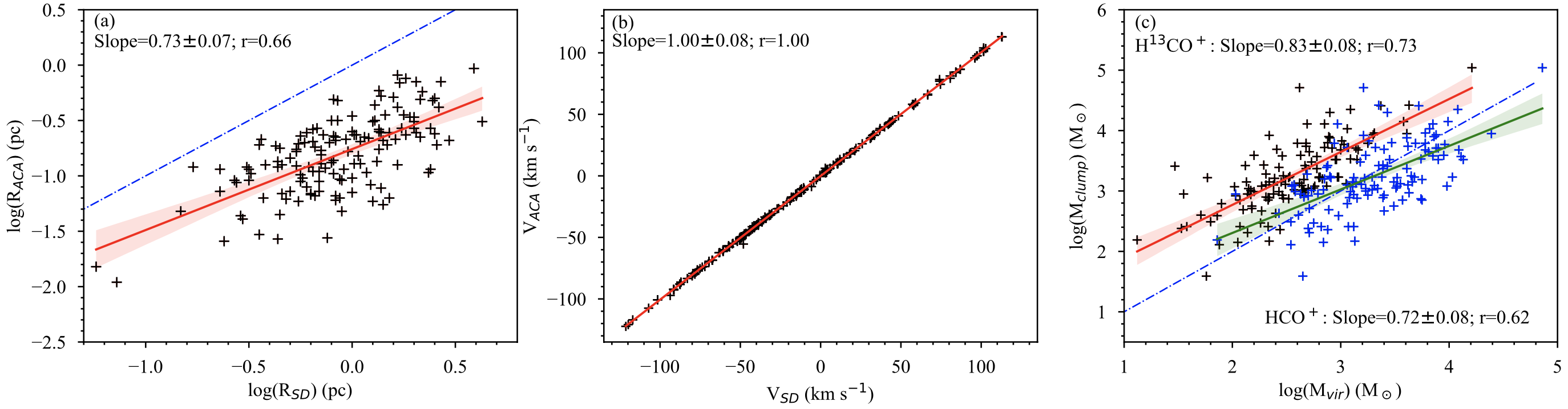
Figure 4: (a) Comparison of effective radii for compact objects in ACA 3 mm continuum observations and effective radii of whole clumps in single dish observations. The blue dashed line represents that the two radii equal to each other. (b) Comparison of systemic velocities in ACA observations and single-dish observations. (c) Comparison of virial masses for compact objects identified in H¹³CO⁺ (black crosses) and HCO⁺ (blue crosses) line emission with total clump masses from single-dish observations. The red and green lines are linear fits. The blue dashed line shows virial masses equaling to clump masses.

We derived virial masses for compact objects identified in H¹³CO⁺ and HCO⁺ line emission following Bertoldi & McKee (1992) and Wu et al. (2010). A correction ($a_{2}\sim 0.9$) for a nonspherical shape in virial analysis is adopted for compact objects with aspect ratios larger than 3 (Bertoldi & McKee, 1992). For the others with smaller aspect ratios, this correction is negligible and has been omitted. We did not derive virial masses for compact objects identified in H¹³CN or HCN because of complications caused by hyperfine structure. The virial masses for objects identified in HCO⁺ are probably overestimated because of line broadening of HCO⁺ resulting from the high optical depth. HCO⁺ also covers a larger region than H¹³CO⁺ due to its lower effective excitation temperature (see Figure 3).

The virial masses ($M_{\rm vir}^{13}$ and $M_{\rm vir}^{12}$) derived from H¹³CO⁺ and HCO⁺ line emission are listed in the last two columns of Table 10. If there are more than one compact objects identified in a source, we simply sum the virial masses of the contributing objects. The virial masses derived from H¹³CO⁺ range from 13 to 16260 $M_{\sun}$ with a median value of 334 $M_{\sun}$. About 90% of the sources have virial masses larger than 100 $M_{\sun}$. The virial masses for the main isotope are considerably larger than those based on the rare isotope. While the HCO⁺ lines are generally optically thick, the other effect is that they extend over a larger region due to much lower effective excitation density. This leads to higher virial masses for HCO⁺.

In Figure 4c, we compare the virial masses with the total clump masses from single-dish measurements (Faúndez et al., 2004; Urquhart et al., 2018). The virial masses are strongly correlated with the total clump masses ($M_{\rm clump}$). The virial masses from H¹³CO⁺ are systematically smaller than the total masses of their natal clumps with a median virial parameter ($\alpha$=$M_{\rm vir}$/$M_{\rm clump}$) of $\sim$0.2. The small value probably reflects the fact that the regions probed by H¹³CO⁺ are smaller than those used to obtain the clump mass from the single-dish data. The virial masses from HCO⁺ are comparable to the total clump masses, with a median virial parameter of $\sim$1.2, indicating that ACA observations of HCO⁺ trace structures similar to those traced by the single-dish millimeter continuum data, which are most likely gravitationally bound.

Small virial parameters have also been reported in many recent measurements of the thermodynamic properties in high-mass star-forming regions (Pillai et al., 2011; Kauffmann et al., 2013; Zhang et al., 2015; Hull & Zhang, 2019), which appear to challenge the picture of star formation in which gas evolves in a state of equilibrium (e.g., Hull & Zhang, 2019). However, in this work and most of previous works magnetic field support were not taken into account in virial analysis. Magnetic support could be comparable to the turbulent and thermal support in high-mass star forming regions, which can bring the dense gas close to a state of equilibrium (Pillai et al., 2011; Sanhueza et al., 2017; Zhang et al., 2015; Liu et al., 2018a, b; Hull & Zhang, 2019; Soam et al., 2019; Tang et al., 2019). More detailed energetics comparison of the gravitational potential energy, turbulent support, thermal pressure, and magnetic support are needed in future analysis of virial equilibrium.

3.3 The relations between infrared luminosities and molecular line luminosities

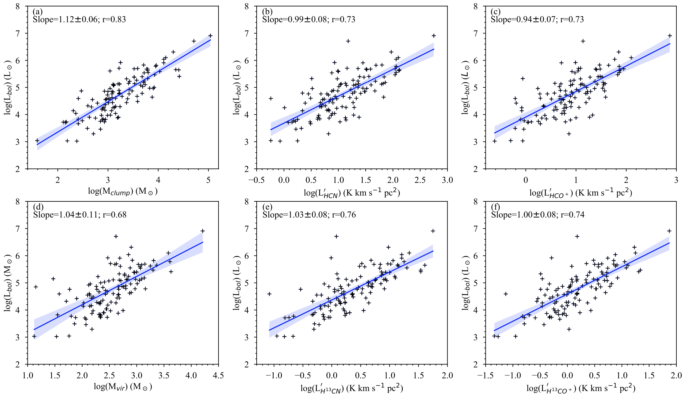
Figure 5: The correlations between $L_{\rm bol}$ and other parameters ($M_{\rm clump}$, $M_{\rm vir}$ derived from H¹³CO⁺ and $L^{\prime}_{\rm mol}$). The solid lines are linear fits. The shadow regions represent 95% confidence levels of the fits. (a) $L_{\rm bol}$ vs. $M_{\rm clump}$; (b) $L_{\rm bol}$ vs. $L^{\prime}_{\rm HCN}$; (c) $L_{\rm bol}$ vs. $L^{\prime}_{\rm HCO^{+}}$; (d) $L_{\rm bol}$ vs. $M_{\rm vir}$ derived from H¹³CO⁺; (e) $L_{\rm bol}$ vs. $L^{\prime}_{\rm H^{13}CN}$; (c) $L_{\rm bol}$ vs. $L^{\prime}_{\rm H^{13}CO^{+}}$.

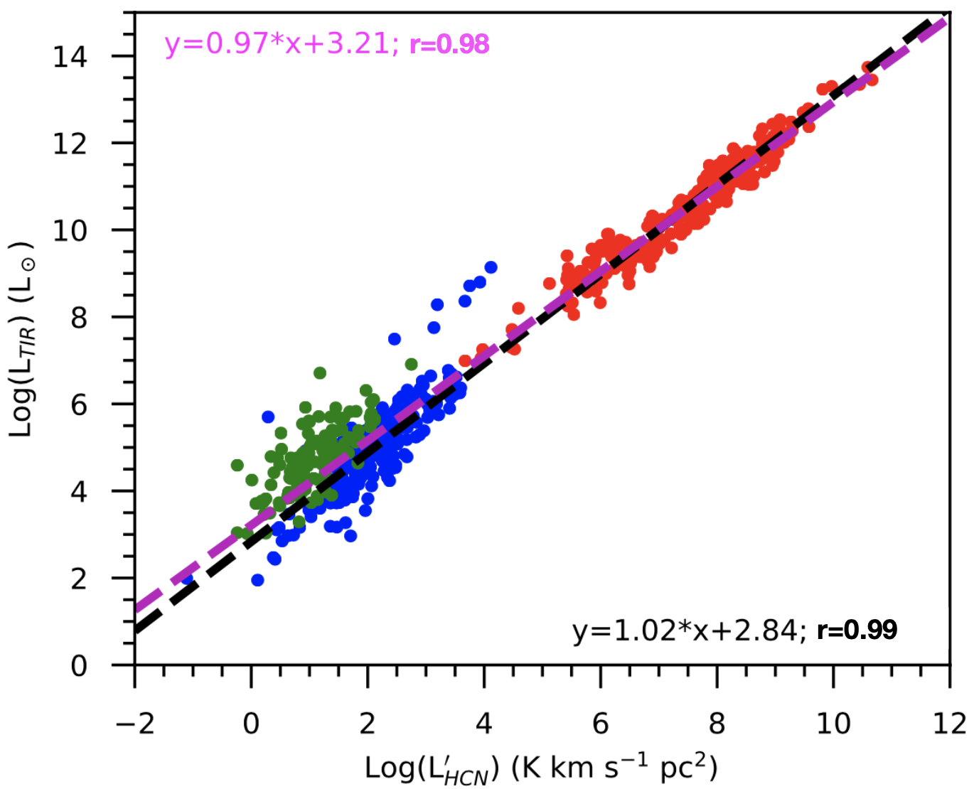
Figure 6: The correlation between $L_{\rm TIR}$ and $L^{\prime}_{\rm HCN}$. The data for compact objects in this study are shown as green filled circles. The data points for Galactic clumps (blue filled circles) and external galaxies (red filled circles) in single-dish observations were compiled by Jiménez-Donaire et al. (2019). The linear fit of all data is shown as the magenta dashed line. The linear fit toward single-dish data is shown as the black dashed line.

In this section, we investigate how the infrared luminosities correlate with molecular line luminosities. Liu et al. (2016) has demonstrated that the bolometric luminosities ($L_{\rm bol}$) from SED fits are nearly identical to the total infrared luminosities ($L_{TIR}$) for this "ATOMS" sample. In this study, we still use $L_{\rm bol}$ (from Faúndez et al., 2004; Urquhart et al., 2018) instead of $L_{\rm TIR}$. The molecular line luminosities ($L^{\prime}_{\rm mol}$) are derived following Solomon et al. (1997) with the total integrated flux density. The $L_{\rm bol}$ and $L^{\prime}_{\rm mol}$ are listed in Table 10. The statistics like minumum, maximum, mean, median and standard deviation of the logarithmic values of $L_{\rm bol}$, $L^{\prime}_{\rm mol}$ and their ratios are summarized in Table 1.

Figure 5 shows the correlations between $L_{\rm bol}$ and other parameters ($M_{\rm clump}$, $M_{\rm vir}$ derived from H¹³CO⁺, and $L^{\prime}_{\rm mol}$). All the relationships appear approximately linear. The correlations are fitted with a linear function using the function "regplot" in the python package Seaborn. The slopes ($a$), intercepts ($b$) and correlation coefficients ($r$) from linear regressions are summarized in Table 2. Since the effective excitation densities of isotopologue lines are significantly larger than their main lines (Shirley, 2015), some models (e.g. Narayanan et al., 2008) would predict that the correlations between $L_{\rm bol}$ and $L^{\prime}_{\rm mol}$ are steeper for isotopologues than that for their main lines. In fact, the relations for isotopologues are not steeper and not even tighter for the "ATOMS" sample (see Figure 5).

The mean log($L_{\rm bol}$/$L^{\prime}_{\rm mol}$) ratios are 4.38, 4.49, 3.67, and 3.86 for H¹³CN, H¹³CO⁺, HCN and HCO⁺, respectively. The $L_{\rm bol}$-to-$L^{\prime}_{\rm HCN}$ and $L_{\rm bol}$-to-$L^{\prime}_{\rm HCO^{+}}$ ratios for compact objects in the "ATOMS" sample seem to be a factor of $\sim$5 larger than the corresponding ratios for Galactic clumps (e.g., Wu et al., 2010; Stephens et al., 2016) and external galaxies (e.g., Jiménez-Donaire et al., 2019) measured with single-dishes. This difference is also understandable because the line emission in our ACA observations is mainly from compact and dense structures (likely to be more gravitationally bound objects). In contrast, line emission in other works with single-dishes also includes extended gas emission or even sub-thermal emission.

In Figure 6, we plot the $L_{\rm TIR}$ (or $L_{\rm bol}$ ) as a function of the $L^{\prime}_{\rm HCN}$ for the "ATOMS" measurements and literature measurements compiled by Jiménez-Donaire et al. (2019) . The literature measurements include single-dish observations toward both Galactic clumps and external galaxies. This scaling relation between $L_{\rm TIR}$ and $L^{\prime}_{\rm HCN}$ is nearly linear spanning almost 10 orders of magnitude in IR and HCN luminosity. The data points in the "ATOMS" measurements are clearly located above the relation determined by data points from single-dish measurements alone, indicating that the ACA observations in the "ATOMS" survey may reveal structures with higher star formation efficiency (SFE) in clouds. These structures in the ACA observations are much denser and more gravitationally bound than those revealed in single dish measurements (see Figure 4c).

Table 1: Statistics of parameters of the 119 sources

Parametersa	Minimum	Maximum	Mean	Median	Std. Deviation
$R_{\rm eff}$	0.15	4.26	1.09	0.84	0.75
$T_{\rm d}$	19	46	29	29	5
$L_{\rm bol}$	3.02	6.91	4.75	4.76	0.77
$M_{\rm clump}$	1.59	5.04	3.24	3.19	0.58
$M_{\rm vir}^{13}$	1.12	4.21	2.53	2.52	0.50
$M_{\rm vir}^{12}$	1.86	4.86	3.30	3.31	0.49
$L^{\prime}_{\rm H^{13}CN}$	-1.08	1.75	0.37	0.31	0.57
$L^{\prime}_{\rm H^{13}CO^{+}}$	-1.34	1.87	0.16	0.14	0.57
$L^{\prime}_{\rm HCN}$	-0.24	2.75	1.07	1.03	0.57
$L^{\prime}_{\rm HCO^{+}}$	-0.62	2.87	0.89	0.89	0.60
$L_{\rm bol}$/$L^{\prime}_{\rm H^{13}CN}$	3.43	6.63	4.38	4.32	0.50
$L_{\rm bol}$/$L^{\prime}_{\rm H^{13}CO^{+}}$	3.26	6.53	4.59	4.57	0.52
$L_{\rm bol}$/$L^{\prime}_{\rm HCN}$	2.47	5.53	3.67	3.63	0.53
$L_{\rm bol}$/$L^{\prime}_{\rm HCO^{+}}$	2.43	5.57	3.86	3.80	0.53
$L^{\prime}_{\rm HCN}$/$L^{\prime}_{\rm HCO^{+}}$	-0.24	0.74	0.18	0.20	0.18
$L^{\prime}_{\rm HCN}$/$L^{\prime}_{\rm H^{13}CN}$	-0.14	1.18	0.70	0.75	0.27
$L^{\prime}_{\rm HCO^{+}}$/$L^{\prime}_{\rm H^{13}CO^{+}}$	-0.03	1.28	0.73	0.77	0.26
$L^{\prime}_{\rm H^{13}CN}$/$L^{\prime}_{\rm H^{13}CO^{+}}$	-0.34	0.69	0.21	0.22	0.20
a Except for $R_{\rm eff}$ and $T_{\rm d}$, the other parameters are logarithmic values.

Table 2: Correlations between parameters

Relation	$a$	$b$	$r$
$M_{\rm clump}$ – $L_{\rm bol}$	1.12(0.06)	1.12(0.21)	0.83
$M_{\rm vir}$ – $L_{\rm bol}$	1.04(0.11)	2.12(0.31)	0.68
$M_{\rm vir}$ – $M_{\rm clump}$	0.83(0.08)	1.14(0.22)	0.73
$L^{\prime}_{\rm HCN}$ – $L_{\rm bol}$	0.99(0.08)	3.68(0.11)	0.73
$L^{\prime}_{\rm HCO^{+}}$ – $L_{\rm bol}$	0.94(0.07)	3.91(0.09)	0.73
$L^{\prime}_{\rm H^{13}CN}$ – $L_{\rm bol}$	1.03(0.08)	4.37(0.07)	0.76
$L^{\prime}_{\rm H^{13}CO^{+}}$ – $L_{\rm bol}$	1.00(0.08)	4.59(0.05)	0.74

4 Discussion

4.1 The dispersion in the $L_{\rm bol}$-to-$L^{\prime}_{\rm mol}$ ratios

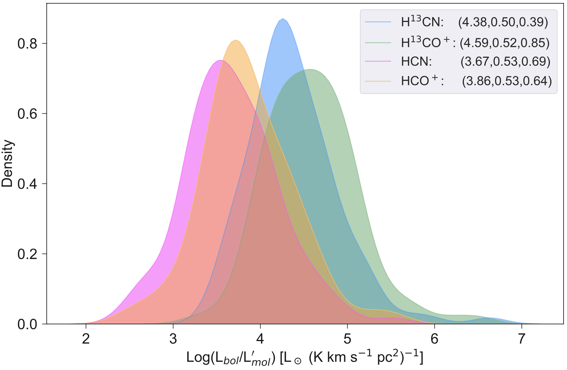
Figure 7: Density distributions of $L_{\rm bol}$-to-$L^{\prime}_{\rm mol}$ ratios, plotted using the function "kdeplot" in the python package Seaborn. The numbers in brackets are mean, standard deviation and asymptotic significance in Kolmogorov-Sminov test of a normal distribution.

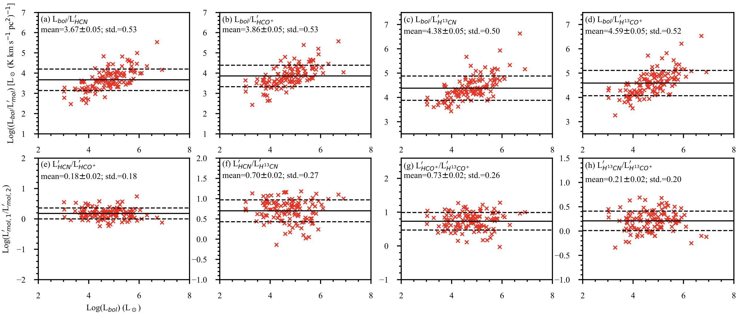
Figure 8: $L_{\rm bol}$-to-$L^{\prime}_{\rm mol}$ ratios (panels a to d) and line luminosity ratios (panels e to h) as a function of bolometric luminosity $L_{\rm bol}$. The solid line is the mean value. The dashed lines show standard deviation. The name of the ratio is labeled at the upper-right corner in each panel.

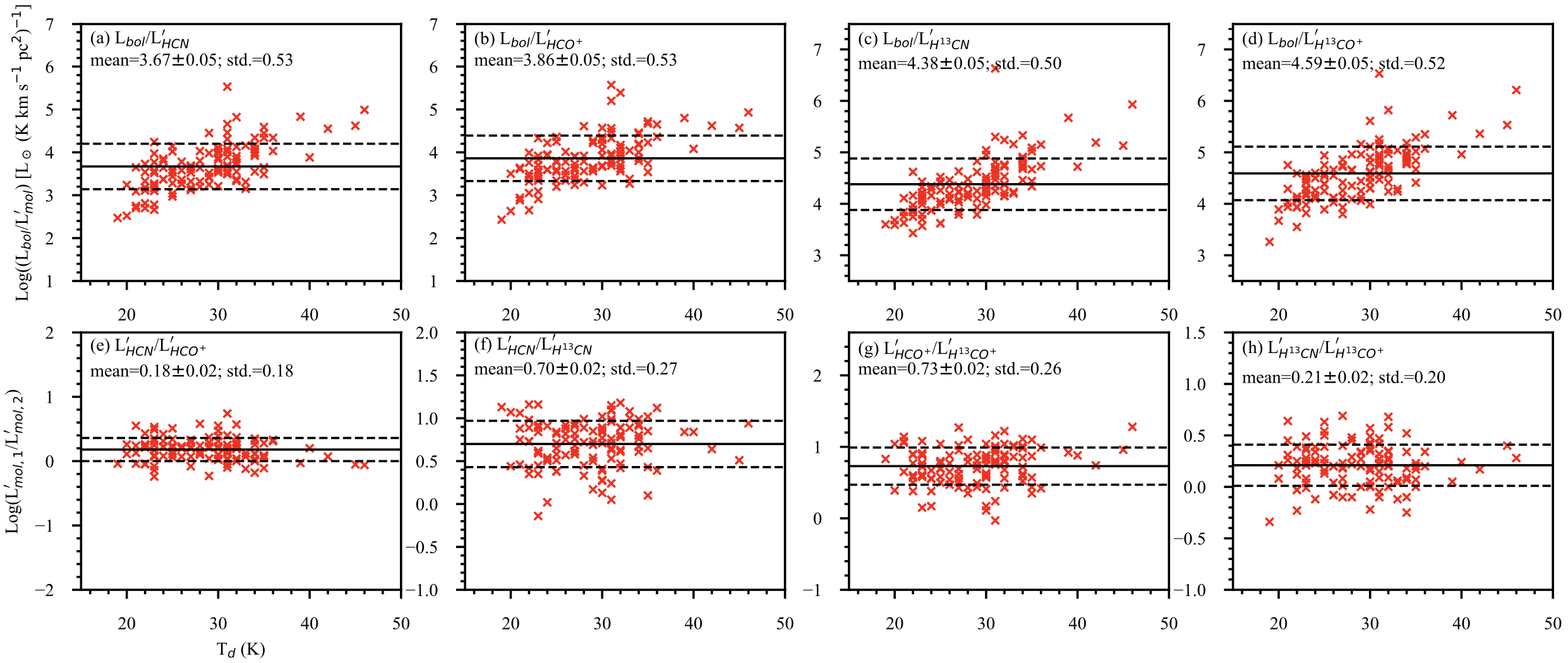
Figure 9: $L_{\rm bol}$-to-$L^{\prime}_{\rm mol}$ ratios (panels a to d) and line luminosity ratios (panels e to h) as a function of dust temperature $T_{\rm d}$. The solid line is the mean value. The dashed lines show standard deviation. The name of the ratio is labeled at the upper-right corner in each panel.

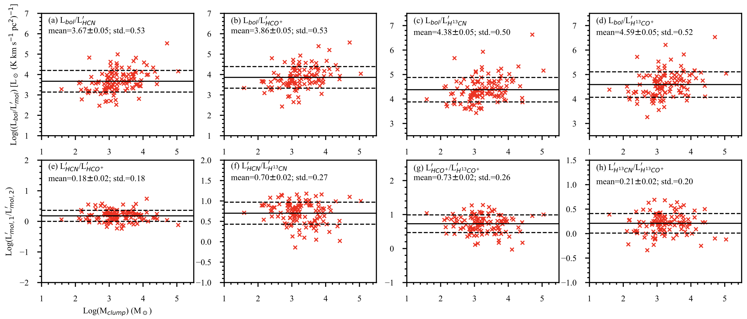
Figure 10: $L_{\rm bol}$-to-$L^{\prime}_{\rm mol}$ ratios (panels a to d) and line luminosity ratios (panels e to h) as a function of clump masses $M_{\rm clump}$. The solid line is the mean value. The dashed lines show standard deviation. The name of the ratio is labeled at the upper-right corner in each panel.

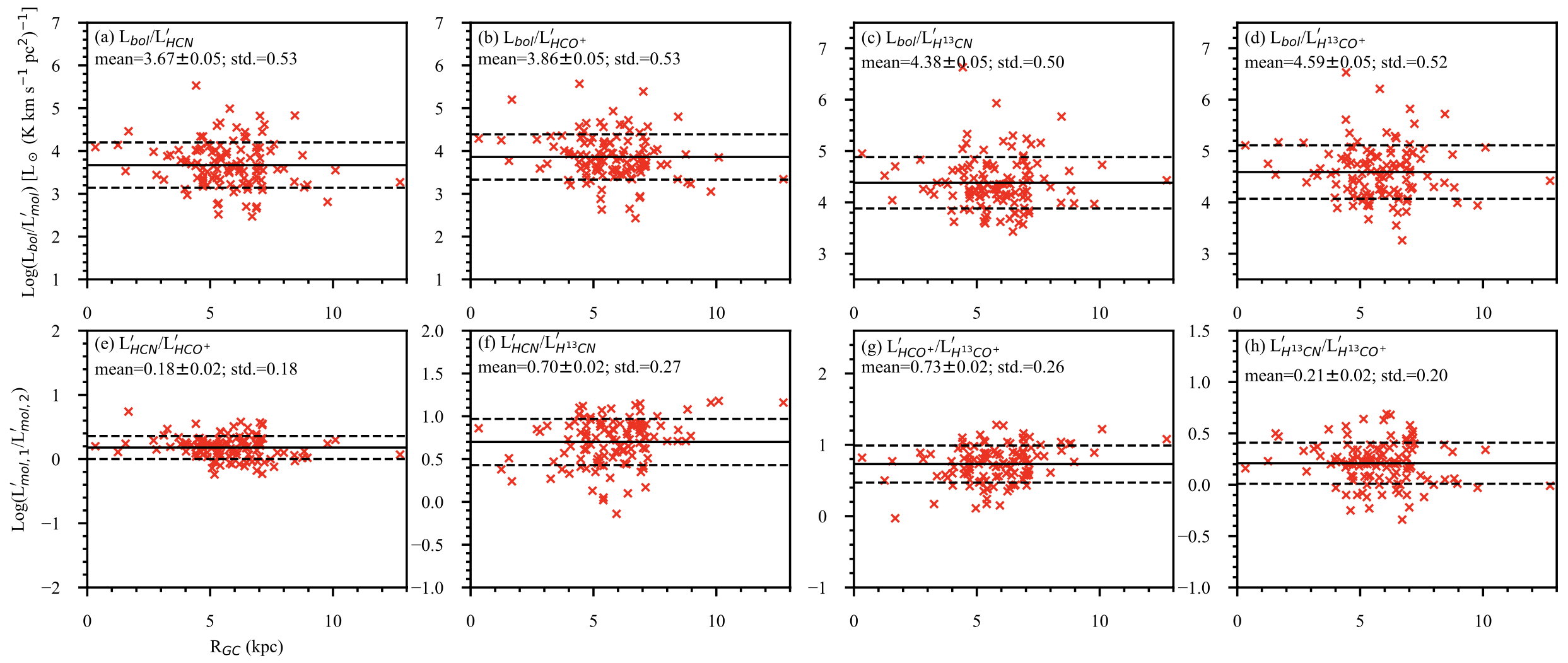
Figure 11: $L_{\rm bol}$-to-$L^{\prime}_{\rm mol}$ ratios and line luminosity ratios as a function of galactocentric distances. The name of the ratio is labeled at the upper-right corner in each panel.

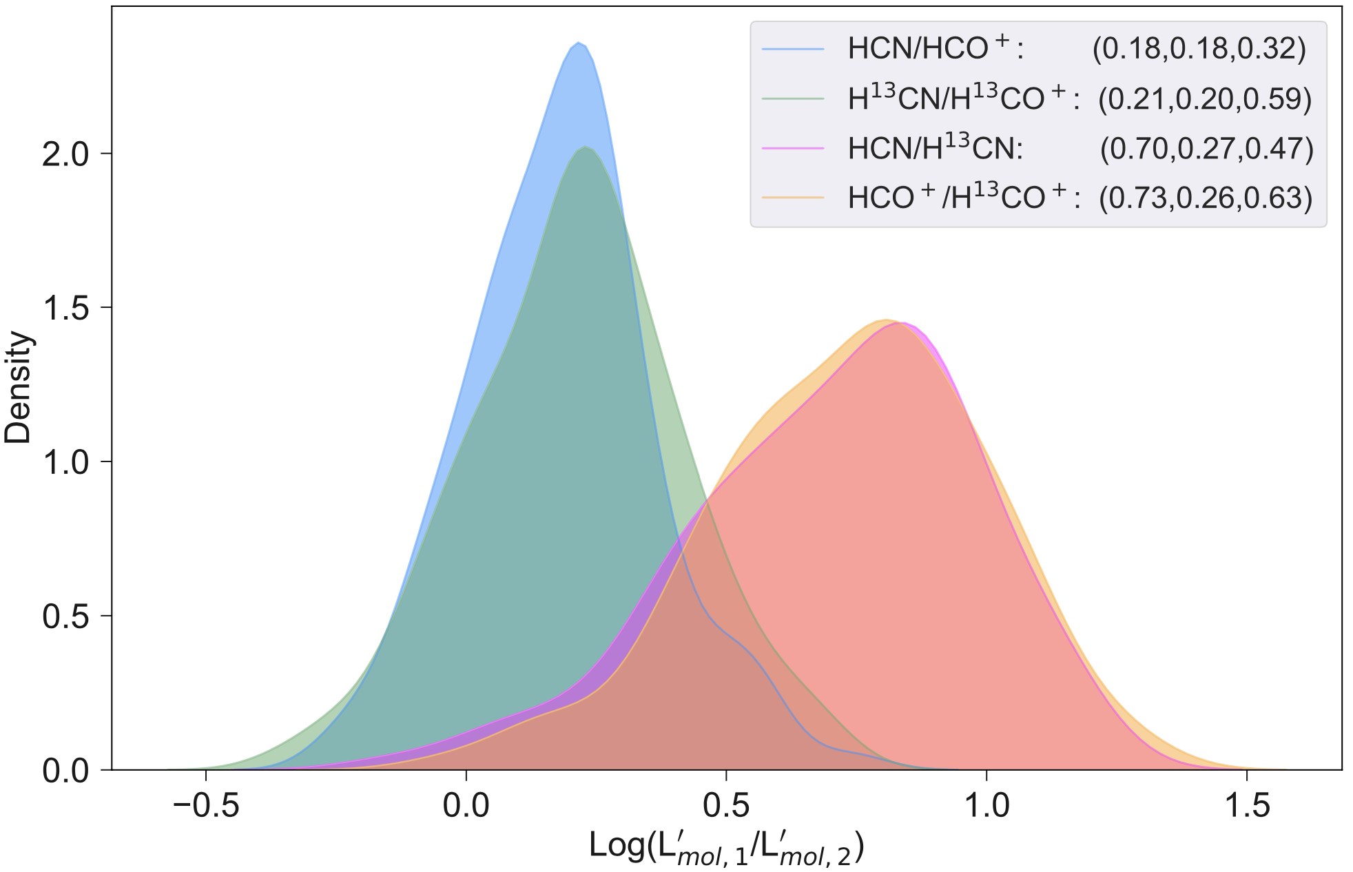
Figure 12: Density distributions of molecular line luminosity ratios, plotted using the function "kdeplot" in the python package Seaborn. The numbers in brackets are mean, standard deviation and asymptotic significance in Kolmogorov-Sminov test of a normal distribution.

We noticed a significant scatter in $L_{\rm bol}$-to-$L^{\prime}_{\rm mol}$ ratios in our data as shown in Figure 7. The standard deviations in distributions of log($L_{\rm bol}$/$L^{\prime}_{\rm mol}$) are around 0.5 for all four molecular line transitions. The scatters in distributions for isotopologues are as large as for their main lines. We test whether the distributions of log($L_{\rm bol}$/$L^{\prime}_{\rm mol}$) follow a normal distribution with Kolmogorov-Sminov test. The null hypothesis is that the distribution of log($L_{\rm bol}$/$L^{\prime}_{\rm mol}$) follows a normal distribution. The tests retain the null hypothesis with asymptotic significances (or P-values; 2-tailed) $\ga$0.4 for the four lines (see Figure 7), indicating that the distributions of log($L_{\rm bol}$/$L^{\prime}_{\rm mol}$) likely follow a normal distribution. Stephens et al. (2016) also reported a significant scatter in $L_{\rm bol}$/$L^{\prime}_{\rm HCN}$ at 1 pc clump-scale. They found that the difference between $L_{\rm bol}$/$L^{\prime}_{\rm HCN}$ for the lowest 10% quantile and the highest 90% quantile is approximately two orders of magnitude. In our data, the difference is smaller, approximately one order of magnitude. It may imply that this ratio does not vary too much in gravitationally bound structures within clumps.

We have also investigated the similarities of distributions of log($L_{\rm bol}$/$L^{\prime}_{\rm mol}$) for different molecular line tracers. In Table 3, we test whether the Log($L_{\rm bol}$/$L^{\prime}_{\rm mol}$) values for two molecular lines could be drawn from the same distribution with Kolmogorov-Sminov test after shifting the distributions by their mean values. The null hypothesis in tests is the shapes of the distributions for Log($L_{\rm bol}$/$L^{\prime}_{\rm mol}$) values are the same for the two molecular lines. With non-parametric tests, we found that the distributions of log($L_{\rm bol}$/$L^{\prime}_{\rm mol}$) for different molecular line tracers are very similar. In particular, the distributions of Log($L_{\rm bol}$/$L^{\prime}_{HCN}$) and Log($L_{\rm bol}$/$L^{\prime}_{HCO^{+}}$) show the highest similarity with asymptotic significances $\sim$0.97 in Kolmogorov-Sminov test. The distributions for isotopologues (H¹³CN and H¹³CO⁺) are also similar to the distributions for their corresponding main lines (HCN and HCO⁺) with asymptotic significance as high as $\sim$0.95 in Kolmogorov-Sminov test. This implies that although the main lines may not trace well the dense structures (cores or filaments) within clumps/clouds (e.g., Kauffmann et al., 2017; Pety et al., 2017; Shimajiri et al., 2017; Liu et al., 2020), they can still reveal the total dense gas masses as well as their isotopologues in statistics.

Panels (a) to (d) in Figure 8 present correlations between the $L_{\rm bol}$-to-$L^{\prime}_{\rm mol}$ ratios and $L_{\rm bol}$. Wu et al. (2005, 2010) suggest that above an infrared luminosity threshold of $\sim 10^{4.5}$ $L_{\sun}$, the $L_{\rm bol}$-to-$L^{\prime}_{\rm mol}$ ratios become constant. However, we do not see such threshold in our data. There seems to be a clear trend that $L_{\rm bol}$-to-$L^{\prime}_{\rm mol}$ ratio increases with $L_{\rm bol}$, spanning four orders of magnitude in $L_{\rm bol}$. This is likely caused by evolutionary effects of the sources, as suggested by Liu et al. (2016) and Stephens et al. (2016). Liu et al. (2016) reported a bimodal behavior in the $L_{\rm bol}$-to-$L^{\prime}_{\rm mol}$ correlations for clumps with different dust temperature, luminosity-to-mass ratio, and virial parameter. More luminous (or more evolved) sources seem to have consumed more gas, leading to higher $L_{\rm bol}$-to-$L^{\prime}_{\rm mol}$ ratios.

More evolved star forming regions might have a higher dust temperature. To test the evolutionary effect, we present in Figure 9 correlations between the $L_{\rm bol}$-to-$L^{\prime}_{\rm mol}$ ratios and dust temperature $T_{\rm d}$. As expected, there is a clear trend that $L_{\rm bol}$-to-$L^{\prime}_{\rm mol}$ increases with T_d. The trend is even more clearly seen for isotopologues. Same trend is seen in Figure 8(a-d) as well where the trend is also more clearly seen in isotopologues.

Clump masses are not as sensitive to the evolutionary effect as bolometric luminosity or dust temperature. Panels (a) to (d) in Figure 10 present correlations between the $L_{\rm bol}$-to-$L^{\prime}_{\rm mol}$ ratios and $M_{\rm clump}$. Indeed, there is no clear trend between $L_{\rm bol}$-to-$L^{\prime}_{\rm mol}$ ratios and $M_{\rm clump}$ that spans three orders of magnitude in $M_{\rm clump}$.

Panels (a) to (d) in Figure 11 present correlations between the $L_{\rm bol}$-to-$L^{\prime}_{\rm mol}$ ratios and galactocentric distances ($R_{\rm GC}$) for different tracers. Jiménez-Donaire et al. (2019) found that $L_{\rm TIR}$-to-$L^{\prime}_{\rm HCN}$ tends to increase with increasing $R_{\rm GC}$ in most of their targeted external galaxies, but with large galaxy-to-galaxy scatter. In our data, however, there is no clear trend for $L_{\rm bol}$-to-$L^{\prime}_{\rm mol}$ ratios against $R_{\rm GC}$, suggesting that this ratio may be constant for gravitationally bound clumps in different Galactic environments.

Table 3: Asymptotic significances (p-value) in non-parametric tests

Distributions	Kolmogorov-Sminova
log($\frac{L_{bol}}{\rm H^{13}CN}$) vs. log($\frac{L_{bol}}{\rm H^{13}CO^{+}}$)	0.69
log($\frac{L_{bol}}{\rm HCN}$) vs. log($\frac{L_{bol}}{\rm HCO^{+}}$)	0.97
log($\frac{L_{bol}}{\rm H^{13}CN}$) vs. log($\frac{L_{bol}}{\rm HCN}$)	0.95
log($\frac{L_{bol}}{\rm H^{13}CO^{+}}$) vs. log($\frac{L_{bol}}{\rm HCO^{+}}$)	0.95
log($\frac{\rm HCN}{\rm HCO^{+}}$) vs. log($\frac{\rm H^{13}CN}{\rm H^{13}CO^{+}}$)	0.89
log($\frac{\rm HCN}{\rm H^{13}CN}$) vs. log($\frac{\rm HCO^{+}}{\rm H^{13}CO^{+}}$)	0.89
a The significance level ($\alpha$-value) is 0.05.

4.2 Variations of molecular line luminosity ratios

Figure 12 plots the density distributions of various molecular line luminosity ratios (or integrated intensity ratios). Interestingly, we found that the distribution of HCN-to-HCO⁺ ratios is very similar to the distribution of H¹³CN-to-H¹³CO⁺ ratios. The non-parametric tests in Table 3 indicate that they can be drawn from a same distribution. It implies that the optical depths of the main lines do not affect the determination of HCN-to-HCO⁺ ratios statistically. The mean HCN-to-HCO⁺ ratios inferred from distributions of log($\frac{\rm HCN}{\rm HCO^{+}}$) and log($\frac{\rm H^{13}CN}{\rm H^{13}CO^{+}}$) are $\sim$1.5 and $\sim$1.6, respectively. This mean HCN-to-HCO⁺ ratio (1.5-1.6) is slightly larger than that in nearby disk galaxies (1.3-1.4; Jiménez-Donaire et al., 2019), Orion B GMC (0.9-1.1; Pety et al., 2017; Shimajiri et al., 2017) and Galactic Plane GMCs (1-1.4; Nguyen-Luong et al., 2020; Wang et al., 2020). The mean HCN-to-HCO⁺ ratio in the “ATOMS" sample is similar to that of Aquila GMC (1.6; Shimajiri et al., 2017). The line ratio of HCN-to-HCO⁺ seems to be sensitive to environments (Pety et al., 2017; Shimajiri et al., 2017). High HCN-to-HCO⁺ ratios have been found in far-UV irradiated environments such as evolved Galactic Hii regions (Nguyen-Luong et al., 2020), AGNs (Aladro et al., 2015) or luminous infrared galaxies (LIRGs; Papadopoulos, 2007). This implies that HCO⁺ abundance is sensitive to the ionization degree of molecular gas. In more far-UV irradiated environments, HCO⁺ is more easily recombined with free electrons, leading to a decrease in its abundance. Increasing HCN-to-HCO⁺ ratios with increasing infrared luminosity have been found in LIRGs (Papadopoulos, 2007). In the Galaxy, more evolved Hii regions also show higher HCN-to-HCO⁺ ratios than infrared dark clouds (Nguyen-Luong et al., 2020). However, in our data, we do not see any trend of HCN-to-HCO⁺ ratios against the $L_{\rm bol}$ spanning four orders of magnitude. This may imply that the majority of HCN and HCO⁺ J=1-0 line emission within the "ATOMS" clumps comes from regions that are not exposed to strong local FUV radiation field. This scenario needs to be tested from detailed analysis of the spatial distributions of molecular line emission inside the clumps, which will be presented in forthcoming works using the high resolution ($\sim 2\arcsec$) ALMA 12-m array data of the "ATOMS" survey (see Liu et al., 2020, for example).

The density distributions for log($\frac{\rm HCN}{\rm H^{13}CN}$) and log($\frac{\rm HCO^{+}}{\rm H^{13}CO^{+}}$) are also quite similar to each other but with large scatter ($\sigma\sim$0.6) in the data (see Figure 12). The large scatter means that the optical depths of the main lines show significant variations among sources. The non-parametric tests in Table 3 confirm that their distributions are nearly the same after shifting the distributions by their mean values, indicating that HCN $J=1-0$ and HCO⁺ $J=1-0$ may have similar opacity in sources of the “ATOMS" sample. The mean HCN-to-H¹³CN ratio and HCO⁺-to-H¹³CO⁺ ratio are $\sim$5.0 and $\sim$5.4, respectively. Assuming an isotopic ¹²C/¹³C ratio of 55 at the median galactocentric distance of 5.8 kpc (Milam et al., 2005), the representative optical depths inferred from these mean ratios are $\sim$12 and $\sim$11 for HCN $J=1-0$ and HCO⁺ $J=1-0$, respectively. Thus the column densities of HCN and HCO⁺ derived from the main lines with optically thin assumption could be underestimated by a factor of $\sim$10 for such high optical depths.

However, there is no trend between molecular line luminosity ratios (HCN-to-HCO⁺, H¹³CN-to-H¹³CO⁺, HCN-to-H¹³CN ratio and HCO⁺-to-H¹³CO⁺) and $L_{\rm bol}$ (see panels (e) to (h) in Figure 8). All these molecular line luminosity ratios seem constant against $L_{\rm bol}$ spanning 4 orders of magnitude in $L_{\rm bol}$. This implies that optical depths (or abundance ratios) of main lines should not affect the interpretation of the slopes in star formation relations. The molecular line luminosity ratios are also not correlated with dust temperature (see panels (e) to (h) in Figure 9) or clump masses (see panels (e) to (h) in Figure 10).

Panels (e) to (h) in Figure 11 present correlations between molecular line luminosity ratios and galactocentric distances ($R_{\rm GC}$) for different tracers. In a survey of nine nearby external galaxies, Jiménez-Donaire et al. (2019) found that there is a decreasing trend of HCN-to-HCO⁺ as a function of galactocentric distances in only two galaxies. No significant changing HCN-to-HCO⁺ ratios are witnessed in the other seven galaxies. There is also no obvious trend for molecular line luminosity ratios against $R_{\rm GC}$ in our data, indicating similar local environments (such as FUV radiation field, density, temperature) for the sources in the "ATOMS" sample.

4.3 Star Formation Efficiencies

Table 4: Statistics of the log of Star Formation Efficiency

		SFR/Mvir(HCO+)				SFR/Mclump				SFR/Mvir(H13CO+)
Number		Mean	Median	Std		Mean	Median	Std		Mean	Median	Std		Selectiona
119		$-2.38$	$-2.33$	$0.63$		$-2.33$	$-2.29$	$0.43$		$-1.62$	$-1.66$	$0.55$		All
75		$-2.09$	$-2.11$	$0.50$		$-2.13$	$-2.10$	$0.36$		$-1.35$	$-1.39$	$0.46$		SFR$>5$
75		$-2.09$	$-2.11$	$0.50$		$-2.13$	$-2.10$	$0.36$		$-1.35$	$-1.39$	$0.46$		SFR$>5$, $r>0.2$
44		$-2.89$	$-2.79$	$0.50$		$-2.66$	$-2.69$	$0.32$		$-2.08$	$-2.13$	$0.35$		SFR$<5$, $r>0.2$
a Selection criteria explained in the text.

Until now, we have dealt with observables, comparing luminosities and masses of various quantities. Now, we engage in the more speculative issues of star formation rate (SFR) and star formation efficiency (SFE). We use the extragalactic definition of SFE: the SFR per unit mass of gas, with units of Myr^-1. On the scale of galaxies and averaged over 5 Myr or longer, the far-infrared luminosity can measure the star formation rate. The relation given in Table 1 of Kennicutt & Evans (2012), and explained in more detail in Hao et al. (2011) and Murphy et al. (2011), can be written in convenient units as

$$SFR=1.49\times 10^{-4}L_{\rm bol}(L_{\sun})\ \mbox{M${}_{\odot}$}\ {\rm Myr}^{-1}$$ (1)

This conversion depends on assumptions about IMF and star formation history, so there is no guarantee that it would apply to the spatial and temporal scales studied in this paper. However, we wish to compare the current results to those of other works that used different indicators of star formation rate. Consequently, we use the equation above to generate estimates of SFR and compare to various mass estimates to gauge the SFE. Comparison of SFE, as opposed to SFR, among samples is best suited to appreciate the dispersion and the relative quality of different predictors of star formation, as shown by Vutisalchavakul et al. (2016); so we focus on SFE here. We further follow Vutisalchavakul et al. (2016) in computing means, medians, and standard deviations of SFE in the log, and present them in Table 4.

As predictors, we consider three estimates of the dense gas mass. These estimates also come with various caveats about what characteristic density they represent (Evans et al., 2020). The first estimate is the masses ($M_{\rm clump}$ in Table 10) of clumps from single dish observations, which were obtained from fitting SEDs using far infrared (IRAS or Herschel) data and (sub-)millimeter continuum data (0.87 mm from Urquhart et al. (2018) or 1.2 mm from Faúndez et al. (2004)). We also use, secondly, the virial masses derived from both HCO⁺ and H¹³CO⁺ ($M_{\rm vir}^{12}$ and $M_{\rm vir}^{13}$in Table 10).

We compare our results for SFE to those of Vutisalchavakul et al. (2016) first. They determined the SFR from the mid-infrared luminosity, again using the extra-galactic relations, which carry the same caveat about IMF and star formation history discussed above. However, they did find that the SFR from the mid-infrared luminosity agreed well with those from the free-free radio continuum, which averages over times of 3 to 10 Myr, as long as the inferred SFR was at least 5 M_⊙ Myr^-1. The criterion of log $L_{\rm bol}\geq 4.5$ used by Wu et al. (2010) implies a star formation rate of $4.7$ M_⊙ Myr^-1, essentially the same criterion. Of the 119 sources in Table 10, 75 satisfy this criterion. Also the sample of Vutisalchavakul et al. (2016) was defined by submillimeter continuum emission, which traced relatively large, somewhat dense clumps. If we make the cut between cores and clumps at a size of 0.2 pc (based on $R_{\rm eff}$ in Table 6), all 75 sources that made the first cut also satisfy the size criteria that make them directly comparable to the sample of Vutisalchavakul et al. (2016).

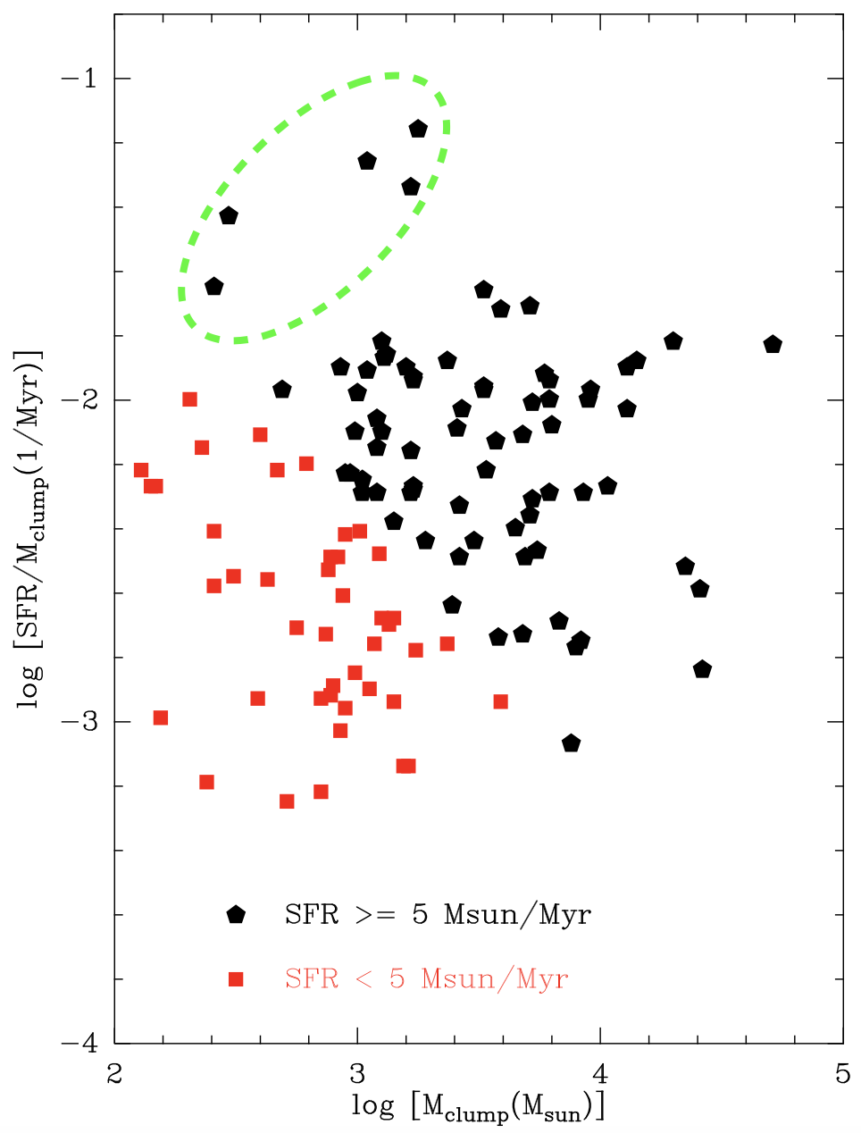
Figure 13: SFR/$M_{\rm clump}$ is plotted versus $M_{\rm clump}$. The red points represent the sources with SFR $<5$ M_⊙ Myr^-1, while the black points represent the sources with SFR $\geq 5$ M_⊙ Myr^-1. The points inside the green dashed ellipse are five outliers with highest dust temperature in the sample.

Figure 13 plots the log of SFE versus the log of $M_{\rm clump}$ for sources that do (black) and do not (red) meet the requirement on SFR of 5 M_⊙ Myr^-1. There are no obvious overall trends in SFE within each sample, but the low luminosity sources lie clearly below the ones above the threshold previously used (Wu et al., 2010; Vutisalchavakul et al., 2016). There are five clear outliers (I09002-4732, I12320-6122, I16562-3959, I17258-3637 and I18139-1842) in Figure 13 at high SFE. These turn out to have unusually large values for $T_{d}$ ($\ga$39 K), as listed in Table 10. To the extent that $T_{d}$ reflects evolutionary state, these sources would be more evolved. If so, a higher fraction of their masses would have been converted into stars, leading to a higher SFE. Table 4 shows the logarithmic means, medians, and standard deviations of the full sample, along with those with the restrictions applied, for three estimates of the mass of dense gas. While the cuts decrease the means and medians, the differences are not large (about 0.3 dex). The last line in Table 4 shows the statistics for the 44 sources that lie below the cut in star formation rate of 5 M_⊙ Myr^-1; their mean and median SFE are much lower, reflecting the fact that log $L_{\rm bol}$ no longer traces the SFR below that value. The SFE based on the HCO⁺ virial mass and the single-dish clump mass are quite similar, but the latter has a smaller dispersion (0.36 dex). The SFE based on the virial mass from H¹³CO⁺ are larger by about 0.8 dex. The mean value for the log of SFE from Vutisalchavakul et al. (2016) is $-1.74\pm 0.50$ for the dense gas, with mean volume density of $n\sim 10^{3}$ cm^-3, 0.38 dex higher than the current sample. In turn, the sample of nearby clouds, where the dense gas mass was determined from the condition that $A_{V}\geq 8$ mag, had a still higher SFE, about $-1.61$. The SFR in the nearby clouds was measured by YSO counting, which is much less sensitive to the IMF and star formation history (Evans et al., 2014).

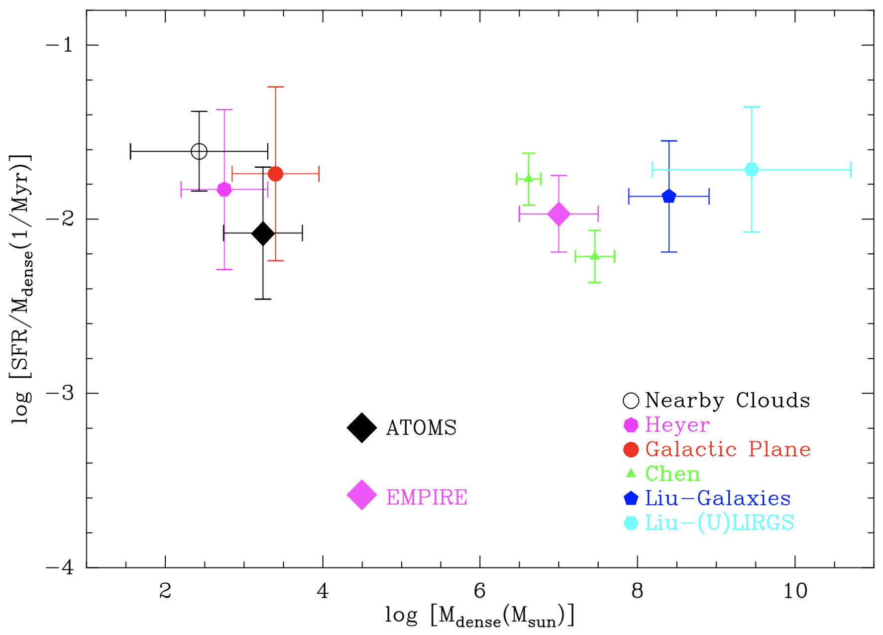
Figure 14: The logarithmic mean SFE (SFR/$M_{\rm dense}$) is plotted versus $M_{\rm dense}$ with both showing the standard deviation in the log. The black diamond is from this work, and the magenta diamond is from the EMPIRE study of nearby galaxies (Jiménez-Donaire et al., 2019). The other points are the same as those in Vutisalchavakul et al. (2016).The red filled circle is from Vutisalchavakul et al. (2016) for Galactic Plane clouds, the empty black circle is from Evans et al. (2014) for nearby clouds. The magenta point (heptagon) comes from Heyer et al. (2016) for a sample of molecular clouds containing 24 $\micron$-based Class I protostars. The two green triangles are from Chen et al. (2015) for resolve giant molecular clouds in M51 (lower one for inner galaxy and higher one for outer galaxy). The blue and cyan points represent the whole normal galaxies and the whole (U)LIRGs, respectively, from Chen et al. (2015).

The masses of dense gas for this sample ($\mbox{$\langle\log(M_{\rm clump})\rangle$}=3.24$; see Table 1) seem to be similar to that of Vutisalchavakul et al. (2016) ($\mbox{$\langle\log(M_{\rm clump})\rangle$}\sim 3.4$). However the sizes of the regions are somewhat smaller with a mean effective clump radius of $1.1$ pc (see Table 1), versus $3.1\pm 2.1$ pc for the sample of Vutisalchavakul et al. (2016) . Consequently the surface and volume densities are higher. The sample selection may play a role. This sample was selected from a survey of CS $J=2-1$ emission (though that survey was itself directed towards IRAS point sources with infrared colors similar to UC Hii regions), thus focusing on relatively dense gas, while the sample of Vutisalchavakul et al. (2016) began with surveys of radio recombination lines, requiring recent formation of massive stars. Based on smaller sizes and higher surface densities, this sample may be younger than the sample of Vutisalchavakul et al. (2016) so a smaller SFE would be expected.

Despite the differences, the values from this paper lie well within the dispersion of values from Vutisalchavakul et al. (2016) and are consistent with the nearly constant SFE from nearby clouds to distant galaxies shown in figure 12 of Vutisalchavakul et al. (2016). We reproduce that figure here (see Figure 14), with the points for ATOMS and for the EMPIRE study (Jiménez-Donaire et al., 2019) added.

5 Conclusions

Some molecular gas tracers (e.g., HCN and HCO⁺) that are commonly used in studies of external galaxies have large optical depths and may not be good tracers of the distribution of dense molecular gas in molecular clouds. In this work, we use the isotopologues of HCN and HCO⁺ to calibrate the relationships between the recent star formation rate (SFR), as traced by the total infrared emission, and the dense molecular gas mass determined from line luminosities ($L^{\prime}_{\rm mol}$). The data used in this work are from ACA observations in the “ATOMS" survey of 146 active Galactic star forming regions. Our main results are summarized as follows:

(1) We extracted 173, 184, 190, 189 and 182 compact objects from 3 mm continuum emission, H¹³CN $J=1-0$, H¹³CO⁺ $J=1-0$, HCN $J=1-0$, and HCO⁺ $J=1-0$ line emission, respectively. The compact objects in 3 mm continuum emission are systematically smaller than compact objects in molecular line emission. Compact sources in HCN $J=1-0$, and HCO⁺ $J=1-0$ line emission have statistically larger effective radii than the compact objects found in the line emission of their isotopologues.

(2) The virial masses of compact objects in H¹³CO⁺ $J=1-0$ line emission are systematically smaller than the total masses of their clumps with a median virial parameter ($\alpha$=$M_{\rm vir}$/$M_{\rm clump}$) of $\sim$0.2, While the virial masses from HCO⁺ are comparable to the total masses of their natal clumps with a median virial parameter of $\sim$1.2. It suggests that our ACA observations most likely detect the gravitationally bound structures inside clumps.

(3) All the correlations between $L_{\rm bol}$, tracing the SFR, and molecular line luminosities $L^{\prime}_{\rm mol}$ of the four transitions (H¹³CN $J=1-0$, H¹³CO⁺ $J=1-0$, HCN $J=1-0$, and HCO⁺ $J=1-0$) appear approximately linear. Line emission of isotopologues shows scatter in their $L_{\rm bol}$-$L^{\prime}_{\rm mol}$ relations as large as that found in their main line emission. Although the main lines may not be good tracers of the spatial distribution of dense gas in molecular clouds (Pety et al., 2017; Shimajiri et al., 2017), they trace the total dense gas masses as well as do their isotopologues.

(4) The density distributions of log($L_{\rm bol}$/$L^{\prime}_{\rm mol}$) for different molecular line tracers show high similarity, indicating that they can be drawn from a same underlying distribution, again confirming that the main lines trace the total dense gas masses as well as do their isotopologues. There seems to be a clear trend between increasing $L_{\rm bol}$-to-$L^{\prime}_{\rm mol}$ ratios and $L_{\rm bol}$ (also $T_{\rm d}$) spanning four orders of magnitude in $L_{\rm bol}$. This is likely caused by evolutionary effects in the sources. $L_{\rm bol}$-to-$L^{\prime}_{\rm mol}$ ratios do not vary with galactocentric distance ($R_{\rm GC}$), suggesting that SFEs remain constant for gravitationally bound clumps in different Galactic environments.

(5) All the molecular line luminosity ratios (HCN-to-HCO⁺, H¹³CN-to-H¹³CO⁺, HCN-to-H¹³CN ratio and HCO⁺-to-H¹³CO⁺) appear constant when compared to $L_{\rm bol}$ over four orders of magnitude in $L_{\rm bol}$. This implies that the large optical depths (or abundance ratios) of main lines do not affect the interpretation of the slopes in star formation relations. There is also no obvious overall trend for molecular line luminosity ratios against $T_{\rm d}$, $M_{\rm clump}$, and $R_{\rm GC}$ in our data.

(6) If we use extragalactic calibrations to convert $L_{\rm bol}$ to a star formation rate and compare it to masses of clumps from single-dish observations or to virial masses from HCO⁺, we can estimate a dense gas star formation efficiency. While this procedure is not fully justified for the scales we are studying, we find that the logarithmic mean SFE is reasonably consistent with other measures of SFE for dense gas, even those using very different tracers or examining very different spatial scales.

Appendix A

Table 5: Selection of Compact objects identified in 3 mm continuum emission^a

IRAS	RA	DEC	$V_{\rm lsr}^{b}$	Distancec	$R_{\rm GC}^{c}$	ID	Offset	$r_{\rm aspect}$	$R_{\rm eff}$	$S_{\rm peak}$	$S_{\rm total}$
			(km s-1)	(kpc)	(kpc)		($\arcsec$,$\arcsec$)		(pc)	(Jy beam-1)	(Jy)
I08076-3556	08:09:32.39	-36:05:13.2	5.9	0.4	8.45	1	(8.56,15.49)	1.37	0.01	0.03	0.03
						2	(4.83,-4.90)	1.07	0.02	0.01	0.02
I08303-4303	08:46:32.90	-43:13:54.0	14.3	2.3	8.96	1	(3.87,7.99)	1.50	0.10	0.06	0.10
I08448-4343	08:48:47.07	-43:54:35.9	3.7	0.7	8.43	1	(2.86,-0.25)	3.86	0.05	0.04	0.09
						2	(21.53,7.53)	1.87	0.05	0.03	0.09
I08470-4243	09:03:32.84	-42:54:31.0	12	2.1	8.83	1	(8.15,4.60)	2.10	0.09	0.07	0.12
I09002-4732	09:11:07.29	-47:44:00.8	3.1	1.2	8.45	1	(0.32,-9.16)	1.08	0.03	3.74	4.26
a The full catalogue is available on line.
b The $V_{\rm lsr}$ values are from Bronfman et al. (1996).
c The distances are from Urquhart et al. (2018) and Faúndez et al. (2004).

Table 6: Selection of compact objects identified in H¹³CO${}^{+}J=1-0^{a}$

IRAS	ID	Offset	$r_{\rm aspect}$	$R_{\rm eff}$	$d_{\rm peak}$	$S_{\rm peak}$	$S_{\rm total}$	$V_{\rm cmp}$	$\sigma$
		($\arcsec$,$\arcsec$)		(pc)	(pc)	(Jy beam-1 km s-1)	(Jy km s-1)	(km s-1)	(km s-1)
I08076-3556	1	(7.26 ,10.15 )	3.39	0.06	0.01	3.12	16.97	6.21	0.28
I08303-4303	1	(9.89 ,10.84 )	1.57	0.26	0.07	8.71	30.18	14.53	1.00
I08448-4343	1	(12.76 ,1.15 )	3.16	0.09	0.03	5.37	21.38	2.78	0.84
	2	(30.80 ,15.93 )	1.77	0.07	0.11	3.62	10.55	5.06	0.66
I08470-4243	1	(4.66 ,17.54 )	1.16	0.22	0.14	4.06	12.96	13.38	0.94
	2	(7.57 ,9.86 )	3.86	0.23	0.05	3.78	16.72	12.06	0.74
I09002-4732	1	(19.98 ,19.19 )	1.70	0.10	0.20	8.48	17.89	2.44	1.08
	2	(12.54 ,-11.26 )	1.52	0.10	0.07	5.33	11.92	4.25	0.70
	3	(18.09 ,-15.62 )	2.74	0.09	0.11	4.33	9.84	2.54	0.62
	4	(1.97 ,-36.41 )	3.50	0.08	0.16	4.44	8.91	3.25	0.57
a The full catalogue is available on line.

Table 7: Selection of compact objects identified in H¹³CN $J=1-0^{a}$

IRAS	ID	Offset	$r_{\rm aspect}$	$R_{\rm eff}$	$d_{\rm peak}$	$S_{\rm peak}$	$S_{\rm total}$
		($\arcsec$,$\arcsec$)		(pc)	(pc)	(Jy beam-1 km s-1)	(Jy km s-1)
I08076-3556	1	(9.76 ,14.74 )	1.34	0.03	0.00	2.79	6.29
I08303-4303	1	(6.08 ,7.36 )	1.19	0.14	0.03	17.00	30.65
I08448-4343	1	(1.27 ,0.58 )	1.63	0.08	0.01	10.10	33.88
	2	(6.53 ,-13.19 )	3.07	0.04	0.05	9.73	18.57
I08470-4243	1	(8.30 ,5.30 )	3.36	0.15	0.01	13.50	33.76
I09002-4732	1	(24.39 ,21.85 )	2.03	0.14	0.23	11.70	41.69
	2	(20.94 ,-12.69 )	4.59	0.08	0.12	4.46	9.71
	3	(13.92 ,-10.52 )	2.36	0.05	0.08	9.52	13.40
	4	(18.83 ,-23.57 )	1.27	0.10	0.14	6.35	14.80
a The full catalogue is available on line.

Table 8: Selection of compact objects identified in HCO⁺ J=1-0^a

IRAS	ID	Offset	raspect	Reff	dpeak	Speak	Stotal	Vcmp	$\sigma$
		($\arcsec$,$\arcsec$)		(pc)	(pc)	(Jy beam-1 km s-1)	(Jy km s-1)	(km s-1)	(km s-1)
HCO+ J=1-0
I08076-3556	1	(10.31 ,13.96 )	1.18	0.04	0.00	21.80	57.20	6.46	1.06
I08303-4303	1	(11.51 ,6.91 )	2.05	0.34	0.09	38.30	182.70	13.93	2.05
I08448-4343	1	(4.88 ,1.10 )	1.53	0.09	0.01	59.80	247.60	2.82	1.92
	2	(24.45 ,11.80 )	1.30	0.08	0.08	37.80	127.00	5.23	1.61
I08470-4243	1	(7.60 ,6.26 )	2.22	0.24	0.02	90.60	325.40	12.78	1.96
I09002-4732	1	(18.83 ,14.75 )	1.13	0.13	0.18	23.50	73.10	-0.69	0.22
	2	(3.11 ,-2.59 )	2.37	0.13	0.04	30.30	104.70	3.28	3.19
	3	(14.81 ,-12.22 )	1.16	0.13	0.09	33.70	115.50	5.57	1.45
a The full catalogue is available on line.

Table 9: Selection of compact objects identified in HCN $J=1-0$^a

IRAS	ID	Offset	$r_{\rm aspect}$	$R_{\rm eff}$	$d_{\rm peak}$	$S_{\rm peak}$	$S_{\rm total}$
		($\arcsec$,$\arcsec$)		(pc)	(pc)	(Jy beam-1 km s-1)	(Jy km s-1)
I08076-3556	1	(8.32 ,15.53 )	1.31	0.03	0.00	21.70	45.16
I08303-4303	1	(7.49 ,8.29 )	1.25	0.19	0.04	78.50	181.90
I08448-4343	1	(3.31 ,0.00 )	1.43	0.07	0.00	95.20	272.50
	2	(24.67 ,11.75 )	1.15	0.06	0.08	48.70	120.40
I08470-4243	1	(8.56 ,3.96 )	2.07	0.17	0.01	158.00	404.00
I09002-4732	1	(23.34 ,24.63 )	3.26	0.16	0.24	34.50	170.20
	2	(17.77 ,-10.99 )	2.25	0.13	0.10	46.40	155.70
	3	(12.29 ,-10.35 )	2.37	0.09	0.07	42.80	92.44
	4	(15.72 ,-27.64 )	1.73	0.17	0.14	32.70	162.70
a The full catalogue is available on line.

Table 10: Parameters of selection from 119 sources^a

IRAS	Reff	Td	log[Lbol]	log[Mclump]	log[L${}^{\prime}_{H^{13}CO^{+}}$]	log[L${}^{\prime}_{H^{13}CN}$]	log[L${}^{\prime}_{HCO^{+}}$]	log[L${}^{\prime}_{HCN}$]	log[M${}_{vir}^{13}$]	log[M${}_{vir}^{12}$]
	(pc)	(K)	(L☉)	(M☉)	(K km s-1 pc2)	(K km s-1 pc2)	(K km s-1 pc2)	(K km s-1 pc2)	(M☉)	(M☉)
I08303-4303	0.32	30	3.83	2.41	-0.16	-0.15	0.60	0.62	2.33	3.07
I08448-4343	0.15	25	3.04	1.59	-1.34	-0.95	-0.30	-0.24	1.76	2.65
I08470-4243	0.32	33	4.04	2.36	-0.25	-0.19	0.77	0.89	2.44	2.88
I09002-4732	0.24	39	4.59	2.41	-1.13	-1.08	-0.21	-0.24	1.58	3.12
I09018-4816	0.44	31	4.72	2.99	-0.21	0.11	0.80	0.82	2.43	3.09
a The full catalogue is available on line.
b Reff, Td, Lbol and Mclump are compiled by Liu et al. (2020), which are adopted from Urquhart et al. (2018) and Faúndez et al. (2004).

Author affiliations:

¹Key Laboratory for Research in Galaxies and Cosmology, Shanghai Astronomical Observatory, Chinese Academy of Sciences, 80 Nandan Road, Shanghai 200030, People’s Republic of China
²Korea Astronomy and Space Science Institute, 776 Daedeokdaero, Yuseong-gu, Daejeon 34055, Republic of Korea
³Department of Astronomy, The University of Texas at Austin, 2515 Speedway, Stop C1400, Austin, TX 78712-1205, USA
⁴University of Science and Technology, Korea (UST), 217 Gajeong-ro, Yuseong-gu, Daejeon 34113, Republic of Korea
⁵Jet Propulsion Laboratory, California Institute of Technology, 4800 Oak Grove Drive, Pasadena, CA 91109, USA
⁶Institute of Astronomy and Astrophysics, Academia Sinica. 11F of Astronomy-Mathematics Building, AS/NTU No. 1, Section 4, Roosevelt Rd., Taipei 10617, Taiwan
⁷Center for Astrophysics $|$ Harvard & Smithsonian, 60 Garden Street, Cambridge, MA 02138, USA
⁸National Astronomical Observatory of Japan, National Institutes of Natural Sciences, 2-21-1 Osawa, Mitaka, Tokyo 181-8588, Japan
⁹Kavli Institute for Astronomy and Astrophysics, Peking University, 5 Yiheyuan Road, Haidian District, Beijing 100871, People’s Republic of China
¹⁰Department of Physics, P.O. Box 64, FI-00014, University of Helsinki, Finland
¹¹Departamento de Astronomía, Universidad de Chile, Las Condes, Santiago, Chile
¹²School of Physics, University of New South Wales, Sydney, NSW 2052, Australia
¹³School of Space Research, Kyung Hee University, Yongin-Si, Gyeonggi-Do 17104, Republic of Korea
¹⁴National Astronomical Observatories, Chinese Academy of Sciences, Beijing, 100012, People’s Republic of China
¹⁵Key Laboratory of Radio Astronomy, Chinese Academy of Science, Nanjing 210008, People’s Republic of China
¹⁶Astronomy Department, University of California, Berkeley, CA 94720, USA
¹⁷Department of Astronomy, Yunnan University, and Key Laboratory of Astroparticle Physics of Yunnan Province, Kunming, 650091, People’s Republic of China
¹⁸IRAP, Université de Toulouse, CNRS, UPS, CNES, Toulouse, France
¹⁹Indian Institute of Space Science and Technology, Thiruvananthapuram 695 547, Kerala, India
²⁰Eötvös Loránd University, Department of Astronomy, Pázmány Péter sétány 1/A, H-1117, Budapest, Hungary
²¹Department of Astronomy, Peking University, 100871, Beijing, People’s Republic of China
²²Departamento de Astronomía, Universidad de Concepción, Av. Esteban Iturra s/n, Distrito Universitario, 160-C, Chile
²³College of Science, Yunnan Agricultural University, Kunming, 650201, People’s Republic of China
²⁴Shanghai Astronomical Observatory, Chinese Academy of Sciences, 80 Nandan Road, Shanghai 200030 People’s Republic of China
²⁵Key Laboratory of Radio Astronomy, Chinese Academy of Sciences, Nanjing 210008, People’s Republic of China
²⁶School of Physics and Astronomy, Sun Yat-sen University, 2 Daxue Road, Zhuhai, Guangdong, 519082, People’s Republic of China

References

- Aladro et al. (2015) Aladro, R., Martín, S., Riquelme, D., et al. 2015, A&A, 579, A101
- Bertoldi & McKee (1992) Bertoldi, F., & McKee, C. F. 1992, ApJ, 395, 140
- Bronfman et al. (1996) Bronfman, L., Nyman, L. -A., May, J., 1996, A&AS, 115, 81
- Chen et al. (2015) Chen, H., Gao, Y., Braine, J., et al., 2015, ApJ, 810, 140
- Evans (1999) Evans, Neal J., II, ARA&A, 37, 311
- Evans et al. (2014) Evans, N. J., Heiderman, A., & Vutisalchavakul, N. 2014, ApJ, 782, 114
- Evans et al. (2020) Evans, Neal J., II, Kim, K.-T., Wu, J.-W., 2020, ApJ, 894, 103
- Faúndez et al. (2004) Faúndez, S., Bronfman, L., Garay, G., et al. 2004, A&A, 426, 97
- Gao & Solomon (2004) Gao, Y., & Solomon, P. M. 2004, ApJ, 606, 271
- García-Burillo et al. (2012) García-Burillo, S., Usero, A., Alonso-Herrero, A., et al. 2012, A&A, 539, A8
- Graciá-Carpio et al. (2006) Graciá-Carpio, J., García-Burillo, S., Planesas, P., & Colina, L. 2006, ApJ, 640, L135
- Greve (2014) Greve, T. R., Leonidaki, I., Xilouris, E. M., et al. 2014, ApJ, 794, 142
- Hao et al. (2011) Hao, C.-N., Kennicutt, R. C., Johnson, B. D., et al. 2011, ApJ, 741, 124
- Heiderman et al. (2010) Heiderman, A., Evans, N. J. II, Allen, L. E., et al., 2010, ApJ, 723, 1019
- Heyer et al. (2016) Heyer, M., Gutermuth, R., Urquhart, J. S., et al. 2016, A&A, 588, A29
- Hoq et al. (2013) Hoq, S., Jackson, J. M., Foster, J. B., et al., 2013, ApJ, 777, 157
- Hull & Zhang (2019) Hull, C. L. H. & Zhang, Q. 2019, FrASS, 6, 3
- Jiménez-Donaire et al. (2017) Jiménez-Donaire, M. J., Bigiel, F., Leroy, A. K., et al., 2017, MNRAS466, 49
- Jiménez-Donaire et al. (2019) Jiménez-Donaire, María J., Bigiel, F., Leroy, A. K., 2019, ApJ, 880, 127
- Juneau et al. (2009) Juneau, S., Narayanan, D. T., Moustakas, J., et al. 2009, ApJ, 707, 1217
- Kauffmann et al. (2013) Kauffmann, J., Pillai, T., & Goldsmith, P. F., 2013, ApJ, 779, 185
- Kauffmann et al. (2017) Kauffmann, J., Goldsmith, P. F., Melnick, G., et al., 2017, A&A, 605, L5
- Kennicutt & Evans (2012) Kennicutt, R. C., & Evans, N. J. 2012, ARA&A, 50, 531
- Lada et al. (2012) Lada, C. J., Forbrich, J., Lombardi, M., et al. 2012, ApJ, 745, 190
- Lada et al. (2010) Lada, C. J., Lombardi, M., & Alves, J. F. 2010, ApJ, 724, 687
- Liu et al. (2015) Liu, D., Gao, Y., Isaak, K., et al. 2015, ApJ, 810L, 14L
- Liu et al. (2016) Liu, T., Kim, K.-T., Yoo, H., et al., 2016, ApJ, 829, 59
- Liu et al. (2018a) Liu, T., Li, P. S., Juvela, M., et al., 2018a, ApJ, 859, 151
- Liu et al. (2018b) Liu, T., Kim, K.-T., Liu, S.-Y., et al., 2018b, ApJ, 869L, 5L
- Liu et al. (2020) Liu, T., Evans, N. J., Kim, K.-T., et al., 2020, MNRAS, 496, 2790
- Lu et al. (2018) Lu, X., Zhang, Q., Liu, H. B., 2018, ApJ, 855, 9
- McMullin et al. (2007) McMullin, J. P., Waters, B., Schiebel, D., et al. 2007, adass XVI, 127
- Milam et al. (2005) Milam, S. N., Savage, C., Brewster, M. A., et al., 2005, ApJ, 634, 1126
- Murphy et al. (2011) Murphy, E. J., Condon, J. J., Schinnerer, E., et al. 2011, ApJ, 737, 67
- Narayanan et al. (2008) Narayanan, D., Cox, T. J., Shirley, Y., Dave, R., Hernquist, L., & Walker, C. K. 2008, ApJ, 684, 996
- Nguyen-Luong et al. (2020) Nguyen-Luong, Q., Nakamura, F., Sugitani, K., et al., 2020, ApJ, 891, 66
- Papadopoulos (2007) Papadopoulos, Padeli P. 2007, ApJ, 656, 792
- Pety et al. (2017) Pety, J., Guzmán, V. V., Orkisz, J. H., et al., 2017, A&A, 599, A98
- Pillai et al. (2011) Pillai, T., Kauffmann, J., Wyrowski, F., et al., 2011, A&A, 530, A118
- Sanhueza et al. (2012) Sanhueza, P., Jackson, J. M., Foster, J. B., et al., 2012, ApJ, 756, 60
- Sanhueza et al. (2017) Sanhueza, P., Jackson, J. M., Zhang, Q., 2017, ApJ, 841, 97
- Shimajiri et al. (2017) Shimajiri, Y., André, P., Braine, J., et al., 2017, A&A, 604, A74
- Shirley (2015) Shirley, Yancy L., 2015, PASP, 127, 299
- Solomon et al. (1997) Solomon, P. M., Downes, D., Radford, S. J. E., & Barrett, J. W. 1997, ApJ, 478, 144
- Soam et al. (2019) Soam, A., Liu, Tie, Andersson, B. -G., 2019, ApJ, 883, 95
- Stephens et al. (2016) Stephens, I. W., Jackson, J. M., & Whitaker, J. S. 2016, ApJ, 824, 29
- Tan et al. (2018) Tan, Q., Gao, Y., Zhang, Z.-Y. et al., 2018, ApJ, 860, 165
- Tang et al. (2019) Tang, Y., Koch, P. M., Peretto, N., et al., 2019, ApJ, 878, 10
- Urquhart et al. (2018) Urquhart, J. S., König, C., Giannetti, A., 2018, MNRAS, 473, 1059
- Vutisalchavakul et al. (2016) Vutisalchavakul, N., Evans, N. J., II, Heyer, M., 2016, ApJ, 831, 73
- Wang et al. (2020) Wang, Y., Beuther, H., Schneider, N., et al., 2020, submitted to A&A, arXiv:2003.05384
- Wu et al. (2005) Wu, J., Evans, N. J., II, Gao, Y., et al. 2005, ApJ, 635, L173
- Wu et al. (2010) Wu, J., Evans, N. J., II, Shirley, Y. L., et al. 2010, ApJS, 188, 313
- Zhang et al. (2015) Zhang, Q., Wang, K., Lu, X., et al., 2015, ApJ, 804, 141
- Zhang et al. (2014) Zhang, Z.-Y., Gao, Y., Henkel, C., et al. 2014, ApJ, 784, L31