How Training Data Impacts Performance in Learning-based Control

Abstract

When first principle models cannot be derived due to the complexity of the real system, data-driven methods allow us to build models from system observations. As these models are employed in learning-based control, the quality of the data plays a crucial role for the performance of the resulting control law. Nevertheless, there hardly exist measures for assessing training data sets, and the impact of the distribution of the data on the closed-loop system properties is largely unknown. This paper derives — based on Gaussian process models — an analytical relationship between the density of the training data and the control performance. We formulate a quality measure for the data set, which we refer to as $\rho$-gap, and derive the ultimate bound for the tracking error under consideration of the model uncertainty. We show how the $\rho$-gap can be applied to a feedback linearizing control law and provide numerical illustrations for our approach.

I INTRODUCTION

Model-based control requires an accurate mathematical description of the plant that is to be controlled. Classical system identification methods postulate parametric models using prior assumptions, and tune their parameters based on observations to achieve high model accuracy [1]. However, these methods are prone to yielding poor models if a wrong parametric structure is assumed, i.e., if insufficient prior knowledge on the system structure is available. This is often the case for highly complex systems, e.g., settings where humans are part of the control loop. In order to overcome these shortcomings, learning-based control employs non-parametric data-driven models, which only require little prior system knowledge in comparison to classical parametric models [2]. Such modeling techniques strongly rely on (potentially noisy) observations, making a formal analysis of the resulting control performance difficult. Hence, these techniques remain too unreliable for safety-critical applications [3].

To overcome this drawback, recent research has focused on the stability of learning-based control approaches using Gaussian process (GP) models [4]. GPs can capture model uncertainty, which allows us to derive probabilistic model error bounds [5]. The applications of GP-based methods range from safe controller optimization for quadrotors [6] to computed torque control in robotics [7] and feedback linearization for aircraft systems [8].

Despite the widespread use of GPs in control, there exist only a few tools to assess the quality of the training set. So far, most measures used to quantify data quality have been based on information-theoretical measures, e.g., information gain [9, 10]. These techniques assess data in global terms, without taking into account locally varying requirements on the data due to the control structure and the task. Since the relationship between data distributions and control performance is largely unknown, random sampling-based approaches have recently been employed to estimate the effect of data on learning-based control systems [11]. However, sampling-based approaches are computationally expensive and provide no direct insight into the interrelation between training data and control error. Therefore, deriving an analytical measure is crucial to improve our understanding of this relationship, and is essential to enhance the efficiency of exploration in active learning, training data selection to implement machine learning with limited computational budget, and cautious control design.

The main contribution of this paper is a novel measure, called $\rho$-gap, to assess training data sets from a control theoretical perspective. Based on the model uncertainty of a GP model, we investigate the uncertainty-dependent Lyapunov stability conditions for a control-affine closed-loop system. This analysis allows insights on how data should be collected, which is becoming particularly useful in exploration tasks where high data-efficiency is required. As an example, we derive a novel uncertainty-dependent ultimate bound of the tracking error for a feedback linearizing control law and show how the density of the training data affects this bound.

The paper is structured as follows: Section II defines the problem setting, after which GP regression and the required model error bounds are introduced in Section III. The control law is presented in Section IV, including the derivation of the ultimate bound and the proposed quality measure of the data. The results are numerically illustrated in Section V, followed by the conclusion in Section VI.

II PROBLEM STATEMENT

We consider a single-input system in the canonical form

$$\dot{x}_{1}=x_{2},\quad\dot{x}_{2}=x_{3},\quad\ldots\quad\dot{x}_{d_{x}}=f(\bm{x})+g(\bm{x})u$$ (1)

with state $\bm{x}=[x_{1}\quad\cdots\quad x_{d_{x}}]^{T}\in\mathbb{X}$ in a compact set $\mathbb{X}\subset\mathbb{R}^{d_{x}}$, input $u\in\mathbb{U}=\mathbb{R}$, and unknown functions $f\colon\mathbb{X}\to\mathbb{R}$ and $g\colon\mathbb{X}\to\mathbb{R}$. Note that we restrict the following analysis to single-input systems due to notational convenience, but our results directly extend to multi-input control-affine systems. We assume that prior models $\hat{f}\colon\mathbb{X}\to\mathbb{R}$ and $\hat{g}\colon\mathbb{X}\to\mathbb{R}$ of the unknown functions are given, and make the following assumptions on the unknown functions and the available data:

Assumption 1

A data set

$$\mathbb{D}=\left\{\bm{z}^{(n)}\coloneqq\begin{bmatrix}\bm{x}^{(n)}\\ u^{(n)}\end{bmatrix},y^{(n)}\!=\!\Delta\left(\bm{z}^{(n)}\right)\!+\!\omega^{(n)}\right\}_{n=1}^{N}$$ (2)

is available, which contains $N$ pairs of noiseless measurements of the state $\bm{x}^{(n)}$ and noisy measurements

$$\Delta(\bm{z})=\Delta(\bm{x},u)\!=\!f(\bm{x})\!-\!\hat{f}(\bm{x})\!+\!(g(\bm{x})\!-\!\hat{g}(\bm{x}))u\!$$ (3)

perturbed by Gaussian noise $\omega^{(n)}\sim\mathcal{N}(0,s_{\mathrm{on}}^{2})$, where $\bm{z}\in\mathbb{X}\times\mathbb{U}\subset\mathbb{R}^{d_{z}}$, and $d_{z}=d_{x}+1$.

Assumption 2

The unknown functions $f(\cdot)$ and $g(\cdot)$ admit Lipschitz constants $L_{f}$ and $L_{g}$, respectively.

Assumption 3

The sign of $g(\cdot)$ is known and constant.

While Assumptions 1 and 2 guarantee the existence of training data, and ensure that the unknown functions are well-behaved, 3 guarantees global controllability, and thereby the existence of a stabilizing control law. We consider the task of tracking a bounded reference trajectory

$$\bm{x}_{d}=\begin{bmatrix}x_{d}&\dot{x}_{d}&\ldots&\frac{\mathrm{d}^{d_{x}-1}x_{d}}{\mathrm{d}t^{d_{x}-1}}\end{bmatrix}^{T},$$ (4)

which can be seen as the generalization of set point regularization, to which our results carry over. We employ a control law $\pi:\mathbb{X}\rightarrow\mathbb{U}$, whose goal is to stabilize the tracking error $\bm{e}=\bm{x}-\bm{x}_{d}$ with the dynamics

$$\dot{e}_{1}=e_{2},\quad\ldots\quad\dot{e}_{d_{x}}=f(\bm{x})+g(\bm{x})\pi(\bm{x})-\frac{\mathrm{d}^{d_{x}-1}x_{d}}{\mathrm{d}t^{d_{x}-1}}.$$ (5)

The control law $\pi(\cdot)$ is based on a model learned by GP regression with a composite kernel

$$k(\bm{z},\bm{z}^{\prime})=k_{f}(\bm{x},\bm{x}^{\prime})+uk_{g}(\bm{x},\bm{x}^{\prime})u^{\prime},$$ (6)

and covariance functions $k_{f},k_{g}:\mathbb{R}^{d_{x}}\times\mathbb{R}^{d_{x}}\rightarrow\mathbb{R}$ as suggested in [12]. Since this kernel reflects the structure of (1), it allows us to recover separate models for $f(\cdot)$ and $g(\cdot)$ [13]. While other kernel functions can also be used for a learning-based control approach [8], they generally do not allow a separation of model components. Since this separation is beneficial for the interpretability and intuitiveness of the relationship between training data and control performance, we focus on composite kernels in the following. The individual covariance functions represent our prior knowledge about the unknown functions.

Assumption 4

Prior knowledge of the function is expressed through prior GPs, i.e., $f(\cdot)\sim\mathcal{GP}(\hat{f}(\bm{x}),k_{f}(\bm{x},\bm{x}^{\prime}))$ and $g(\cdot)\sim\mathcal{GP}(\hat{g}(\bm{x}),k_{g}(\bm{x},\bm{x}^{\prime}))$.

This assumption imposes a probability distribution on the function space, which is shaped by the prior mean functions $\hat{f}(\cdot),\hat{g}(\cdot)$ and the kernel functions $k_{f}(\cdot,\cdot),k_{g}(\cdot,\cdot)$. Thereby, it implicitly requires that the covariance kernels and prior mean functions are chosen suitably, i.e., $f(\cdot),g(\cdot)$ must be expressible in terms of those functions [5].

While the stability of control laws has been investigated under these assumptions [8, 12], the derived ultimate bounds do not depend on the training data. Hence, the impact of training data on the performance of the learning-based controller is unknown. We address this issue by developing a flexible measure of the quality of training data with respect to the control performance. In order to illustrate the flexibility of the proposed quality measure, we derive a novel uncertainty-dependent ultimate tracking error bound for feedback linearizing control of systems with both $f(\cdot)$ and $g(\cdot)$ unknown, and apply our quality measure to this problem.

III GAUSSIAN PROCESS REGRESSION

A Gaussian process defines a distribution $\mathcal{GP}(\mu_{0}(\bm{z}),k(\bm{z},\bm{z}^{\prime}))$ over functions $h:\mathbb{R}^{d_{z}}\rightarrow\mathbb{R}$ with prior mean $\mu_{0}:\mathbb{R}^{d_{z}}\rightarrow\mathbb{R}$ and covariance $k:\mathbb{R}^{d_{z}}\times\mathbb{R}^{d_{z}}\rightarrow\mathbb{R}$, such that any finite number of evaluation points $\{\bm{z}_{1},\ldots,\bm{z}_{m}\}$, $m\in\mathbb{N}$ is assigned a Gaussian distribution [14]. The prior mean function incorporates known parametric models into the regression, while the kernel $k(\cdot,\cdot)$ encodes information about the structure of $h(\cdot)$. Due to the structure of the modeling error $h(\cdot)=\Delta(\cdot)$ in (3), we employ a prior mean function $\mu_{0}(\bm{z})=\hat{f}(\bm{x})+\hat{g}(\bm{x})u$ and the composite kernel $k(\cdot,\cdot)$ defined in (6). For the components of the composite kernel $k(\cdot,\cdot)$, we use squared exponential kernels $k_{f}(\cdot,\cdot)$ and $k_{g}(\cdot,\cdot)$, defined as

$$k_{f,g}(\bm{x},\bm{x}^{\prime})=s_{f,g}^{2}\exp\left(-\frac{\|\bm{x}-\bm{x}^{\prime}\|}{2l_{f,g}^{2}}\right),$$ (7)

where $s_{f}^{2},s_{g}^{2}\in\mathbb{R}_{+,0}$ and $l_{f},l_{g}\in\mathbb{R}_{+}$ denote the signal variances and length scales, respectively. Using the covariance function $k(\cdot,\cdot)$, the elements of the data covariance matrix $\bm{K}$ and the kernel vector $\bm{k}(\bm{z})$ at a test point $\bm{z}$ are given by $K_{nn^{\prime}}=k(\bm{z}^{(n)},\bm{z}^{(n^{\prime})})$ and $k_{n}(\bm{z})=k(\bm{z}^{(n)},\bm{z})$, respectively. Based on these definitions, the probability of $h(\bm{z})$ conditioned on the training data $\mathbb{D}$ as well as the test point $\bm{z}$ is Gaussian with mean and variance

$$\mu(\bm{z}) =\mu_{0}(\bm{z})+\bm{k}^{T}(\bm{z})\left(\bm{K}+s_{\mathrm{on}}^{2}\bm{I}_{N}\right)^{-1}\bm{y}$$ (8)

$$\sigma^{2}(\bm{z}) =k(\bm{z},\bm{z})-\bm{k}^{T}(\bm{z})(\bm{K}+s_{\mathrm{on}}^{2}\bm{I}_{N})^{-1}\bm{k}(\bm{z}),$$ (9)

where the training outputs $y^{(n)}$ are concatenated in the target vector $\bm{y}=\begin{bmatrix}y^{(1)}&\ldots&y^{(N)}\end{bmatrix}^{T}$. Due to the definition of the composite kernel (6), we can express the kernel vector as $\bm{k}(\bm{z})=\bm{k}_{f}(\bm{x})+\bm{U}\bm{k}_{g}(\bm{x})u$, where $\bm{U}=\mathrm{diag}([u^{(1)}\ \ldots\ u^{(N)}])$ and the elements of $\bm{k}_{f}(\cdot)$ and $\bm{k}_{g}(\cdot)$ are defined as $k_{f,n}(\bm{x})=k_{f}(\bm{x}^{(n)},\bm{x})$ and $k_{g,n}(\bm{x})=k_{g}(\bm{x}^{(n)},\bm{x})$, respectively. By exploiting this structure, it is possible to recover the posterior GPs for $f(\cdot)$ and $g(\cdot)$ from the regression, and derive probabilistic uniform error bounds that depend on the posterior standard deviation, as shown in the following theorem:

Lemma 1

Consider a GP with composite kernel given by (6), a training data set $\mathbb{D}$ and functions $f(\cdot)$, $g(\cdot)$, $\hat{f}(\cdot)$ and $\hat{g}(\cdot)$ satisfying Assumptions 1, 2 and 4. For any $\delta\in(0,1)$ and $\tau\in\mathbb{R}_{+}$, it holds that

$$P\!\left(\!|f\!(\bm{x})\!-\!\mu_{\!f}\!(\bm{x})|\!\leq\!\sqrt{\!\beta\!(\tau)}\sigma_{\!f}\!(\bm{x})\!+\!\gamma_{\!f}\!(\tau)\!,\!\forall\bm{x}\!\in\!\mathbb{X}\!\right) \!\geq\!1\!-\!\delta\!$$ (10)

$$\!P\!\left(\!|g(\bm{x})\!-\!\mu_{\!g}\!(\bm{x})|\!\leq\!\sqrt{\!\beta\!(\tau)}\sigma_{\!g}\!(\bm{x})\!+\!\gamma_{\!g}\!(\tau)\!,\!\forall\bm{x}\!\in\!\mathbb{X}\!\right) \!\geq\!1\!-\!\delta\!,\!$$ (11)

with mean and variance components

$$\mu_{f}(\bm{x}) \!=\!\hat{f}(\bm{x})\!+\!\bm{k}_{f}^{T}(\bm{x})(\bm{K}\!+\!s_{\mathrm{on}}^{2}\bm{I}_{N})^{-1}\bm{y}$$ (12)

$$\mu_{g}(\bm{x}) \!=\!\hat{g}(\bm{x})\!+\!\bm{k}_{g}^{T}(\bm{x})\bm{U}(\bm{K}\!+\!s_{\mathrm{on}}^{2}\bm{I}_{N})^{-1}\bm{y}$$ (13)

$$\sigma_{f}^{2}(\bm{x}) \!=\!k_{f}(\bm{x},\bm{x})\!-\!\bm{k}_{f}^{T}(\bm{x})(\bm{K}\!+\!s_{\mathrm{on}}^{2}\bm{I}_{N})^{-1}\bm{k}_{f}(\bm{x})$$ (14)

$$\sigma_{g}^{2}(\bm{x}) \!=\!k_{g}(\bm{x},\bm{x})\!-\!\bm{k}_{g}^{T}(\bm{x})\bm{U}(\bm{K}\!+\!s_{\mathrm{on}}^{2}\bm{I}_{N})^{-1}\bm{U}\bm{k}_{g}(\bm{x}),$$ (15)

and parameters

$$\beta(\tau) =2d_{x}\log\left(1+\frac{r_{0}}{\tau}\right)-2\log(\delta)$$ (16)

$$\gamma_{f}(\tau) =(L_{\mu_{f}}+L_{f})\tau+\sqrt{\beta(\tau)L_{\sigma_{f}^{2}}\tau}$$ (17)

$$\gamma_{g}(\tau) =(L_{\mu_{g}}+L_{g})\tau+\sqrt{\beta(\tau)L_{\sigma_{g}^{2}}\tau}.$$ (18)

Here, $L_{\mu_{f}}$, $L_{\mu_{g}}$, $L_{\sigma_{f}^{2}}$ and $L_{\sigma_{g}^{2}}$ are the Lipschitz constants of the mean and variance components, respectively, and $r_{0}=\max_{\bm{x},\bm{x}^{\prime}\in\mathbb{X}}\|\bm{x}-\bm{x}^{\prime}\|$ denotes the maximum diameter of $\mathbb{X}$.

Proof:

It has been shown in [13] that the independent components $f(\cdot)$ and $g(\cdot)u$ can be inferred by

$$f(\bm{x})|\mathbb{D} \sim\mathcal{N}(\mu_{f}(\bm{x}),\sigma_{f}^{2}(\bm{x}))$$ (19)

$$g(\bm{x})u|\mathbb{D} \sim\mathcal{N}(\mu_{g}(\bm{x})u,u^{2}\sigma_{g}^{2}(\bm{x}))$$ (20)

due to the structure of the kernel. Since $g(\bm{x})u$ depends linearly on $u$, we can extract

$$g(\bm{x})|\mathbb{D} \sim\mathcal{N}(\mu_{g}(\bm{x}),\sigma_{g}^{2}(\bm{x})).$$ (21)

Based on these identities, it is straightforward to adapt [5, Theorem 3.1] to obtain the uniform error bounds (10), (11).∎

It is well known from scattered data approximation [15] that training data which covers $\mathbb{X}$ well typically leads to small posterior variances, thereby implying that the learned model has a high accuracy. Lemma 1 also exhibits this behavior, even though it additionally depends on the constants $\gamma_{f}(\tau)$ and $\gamma_{g}(\tau)$. Since these constants can be made arbitrarily small by reducing the value of $\tau$, their effect is usually negligible. In fact, bounds (10) and (11) can be shown to converge to $0$ under weak assumptions [5].

IV QUALITY ASSESSMENT OF TRAINING DATA FOR LEARNING-BASED CONTROL

IV-A Lyapunov-based Quality Assessment

Although GPs are frequently used in control design, the relationship between training data and the resulting performance of a control law $u=\pi(\bm{x})$ has barely been analyzed. Therefore, there is typically little insight on where training samples should be placed to achieve the highest improvement in control performance. In the sequel, we measure the control performance using a Lyapunov function $V:\mathbb{R}^{d_{x}}\rightarrow\mathbb{R}_{+,0}$. Therefore, we investigate the time derivative of the Lyapunov function for systems defined in (1) given by

$$\!\dot{V}(\bm{e})=$$

$$\!\sum\limits_{i=1}^{d_{x}-1}\!\frac{\partial V(\bm{e})}{\partial e_{i}}e_{i+1}\!\!+\!\frac{\partial V(\bm{e})}{\partial e_{d_{x}}}\!\left(\!\!f(\bm{x})\!+\!g(\bm{x})\pi(\bm{x})\!-\!\frac{\mathrm{d}^{d_{x}}x_{d}}{\mathrm{d}t^{d_{x}}}\!\!\right)\!.\!$$ (22)

By employing a Gaussian process model, as presented in Section III, and exploiting the uniform error bound for GPs from Lemma 1, we can bound this derivative by

$$\dot{V}(\bm{e}) \leq\dot{V}_{\mathrm{nom}}(\bm{e})+\dot{V}_{\sigma_{f}}(\bm{e})+\dot{V}_{\sigma_{g}}(\bm{e}),$$ (23)

where the nominal component of the Lyapunov derivative is computed based on the GP mean function as

$$\!\dot{V}_{\mathrm{nom}}(\bm{e})=$$

$$\!\sum\limits_{i=1}^{d_{x}\!-\!1}\!\!\frac{\partial V(\bm{e})}{\partial e_{i}}e_{i+1}\!\!+\!\frac{\partial V(\bm{e})}{\partial e_{d_{x}}}\!\!\left(\!\!\mu_{f}\!(\bm{x})\!+\!\mu_{g}\!(\bm{x})\pi(\bm{x})\!-\!\frac{\mathrm{d}^{d_{x}}x_{d}}{\mathrm{d}t^{d_{x}}}\!\!\right)\!\!.\!$$ (24)

The uncertain component of $\dot{V}(\cdot)$ is separated into components for the uncertainty about $f(\cdot)$ and $g(\cdot)$, given by

$$\dot{V}_{\sigma_{f}}(\bm{e}) =\left|\frac{\partial V(\bm{e})}{\partial e_{d_{x}}}\right|(\sqrt{\beta(\tau)}\sigma_{f}(\bm{x})+\gamma_{f}(\tau))$$ (25)

$$\dot{V}_{\sigma_{g}}(\bm{e}) =\left|\frac{\partial V(\bm{e})}{\partial e_{d_{x}}}\right|(\sqrt{\beta(\tau)}\sigma_{g}(\bm{x})+\gamma_{g}(\tau))|\pi(\bm{x})|.$$ (26)

The nominal component of the Lyapunov function derivative does not depend on the uncertainty. Hence, it does not provide insight into the relationship between training data and control performance. In contrast, $\dot{V}_{\sigma_{f}}(\cdot)$ and $\dot{V}_{\sigma_{g}}(\cdot)$ directly depend on the GP posterior standard deviations, and thereby on the training data density. In order to measure this density in a flexible way, we introduce the $M$-fill distance, inspired by classical concepts from scattered data approximation [15].

Definition 1

The $M$-fill distance $\phi_{\bar{u}\!,\underaccent{\bar}{u}\!,M}(\bm{x})$ at a point $\bm{x}\in\mathbb{X}$ is defined as the minimum radius $\varphi$ of a ball with center $\bm{x}$, such that the ball contains $M$ training samples $\bm{z}^{(\!n\!)}$ with control inputs $\underaccent{\bar}{u}\!\leq\!|u^{(\!n\!)}|\!\leq\!\bar{u}$ for some $\underaccent{\bar}{u},\bar{u}\in\mathbb{R}_{+,0}$, i.e.,

$$\!\phi_{\bar{u}\!,\underaccent{\bar}{u}\!,M}(\bm{x})\! =\!\min\limits_{\varphi\in\mathbb{R}_{+,0}}\varphi$$ (27a)

s.t. $$\!\left|\!\left\{\!\bm{z}\!^{(\!n\!)}\!\!\in\!\mathbb{D}\!\!:\!\|\bm{x}\!-\!\bm{x}\!^{(\!n\!)}\!\|\!\leq\!\varphi\!\wedge\!\underaccent{\bar}{u}\!\leq\!|u\!^{(\!n\!)}\!|\!\leq\!\bar{u}\!\right\}\!\right|\!\geq\!M\!.$$ (27b)

The $M$-fill distance $\phi_{\bar{u},\underaccent{\bar}{u},M}(\bm{x})$ measures the distance to the $M$ closest training samples, where the parameter $M$ is used to adapt $\phi_{\bar{u},\underaccent{\bar}{u},M}(\bm{x})$ to the total number of training samples $N$. Intuitively, one should choose $M\ll N$, such that only training points in the proximity of $\bm{x}$ are relevant for $\phi_{\bar{u},\underaccent{\bar}{u},M}(\bm{x})$, thereby making it a local measure of the data density. A low $M$-fill distance implies a high data density and indeed, upper bounds for $\phi_{\bar{u},\underaccent{\bar}{u},M}(\bm{x})$ can be derived to guarantee a desired behavior $\xi_{f}(\cdot)$ and $\xi_{g}(\cdot)$ for $\dot{V}_{\sigma_{f}}(\cdot)$ and $\dot{V}_{\sigma_{g}}(\cdot)$, respectively.

Theorem 1

If the $M$-fill distance $\phi_{\bar{u}_{f},0,M}\!(\cdot)$ satisfies

$$\phi_{\bar{u}_{f},0,M}^{2}(\bm{x})\leq\bar{\phi}_{f}^{2}(\bm{x})+\theta_{f}$$ (28)

for all $\bm{x}\in\mathbb{X}$, where

$$\bar{\phi}_{f}^{2}(\bm{x})\! =-l_{f}^{2}\!\log\!\left(\!\!1\!-\!\frac{\left(\xi_{f}(\bm{e})-\gamma_{f}(\tau)\left|\frac{\partial V(\bm{e})}{\partial e_{d_{x}}}\right|\right)^{2}}{\beta(\tau)s_{f}^{2}\left|\frac{\partial V(\bm{e})}{\partial e_{d_{x}}}\right|^{2}}\!\right)$$ (29)

$$\theta_{f} =-l_{f}^{2}\log\left(\!\!\frac{Ms_{f}^{2}\!+\!Ms_{g}^{2}\bar{u}_{f}^{2}\!+\!s_{\mathrm{on}}^{2}}{Ms_{f}^{2}}\!\!\right)$$ (30)

for any $\bar{u}_{f}\!\in\!\mathbb{R}_{+,0}$, $M\!\in\!\mathbb{N}$, and $\xi_{f}(\bm{e})\!>\!\gamma_{f}(\tau)|\partial V(\bm{e})/\partial e_{d_{x}}|$,

then, $\dot{V}_{\sigma_{f}}(\bm{e})\!\leq\!\xi_{f}(\bm{e})$, $\forall\bm{x}\!\in\!\mathbb{X}$.

Proof:

In order to prove this lemma, we have to bound the posterior standard deviation $\sigma_{f}(\bm{x})$. Following the approach introduced in [16], this is achieved by considering only $M$ training samples $\bm{z}^{(n)}$ within distance $\phi_{\bar{u},\underaccent{\bar}{u},M}(\bm{x})$ to $\bm{x}$ such that the posterior variance is bounded by

$$\sigma_{f}^{2}(\bm{x})\leq s_{f}^{2}-\frac{\|\bm{k}_{f,M}(\bm{x})\|^{2}}{\lambda_{\max}(\bm{K}_{M})+s_{\mathrm{on}}^{2}},$$ (31)

where $\bm{k}_{f,M}(\bm{x})$ and $\bm{K}_{M}$ denote the covariance vector and matrix based on these $M$ samples and $\lambda_{\max}(\bm{K}_{M})$ denotes the maximum eigenvalue. Application of the Gershgorin theorem allows us to bound the maximum eigenvalue by

$$\lambda_{\max}(\bm{K}_{M})\leq M(s_{f}^{2}+\bar{u}_{f}^{2}s_{g}^{2}).$$ (32)

Since we have $\|\bm{k}_{f\!,M}\!(\bm{x})\|^{2}\!\geq\!\!Ms_{f}^{4}\!\exp(\!-\phi_{\bar{u}_{f}\!,0,M}^{2}\!(\bm{x})/l_{f}^{2})$, we obtain the posterior variance bound

$$\sigma_{f}^{2}(\bm{x}) \leq s_{f}^{2}-\frac{s_{f}^{4}\exp\left(-\frac{\phi_{\bar{u}_{f}\!,0,M}^{2}(\bm{x})}{l_{f}^{2}}\right)}{s_{f}^{2}+\bar{u}_{f}^{2}s_{g}^{2}+\frac{s_{\mathrm{on}}^{2}}{M}}.$$ (33)

Substituting this expression into (25) and solving for $\phi_{\bar{u}_{f}\!,0,M}^{2}(\bm{x})$ yields the desired result. ∎

Corollary 1

If the $M$-fill distance $\phi_{\bar{u}_{g},\underaccent{\bar}{u}_{g},M}(\cdot)$ satisfies

$$\phi^{2}_{\bar{u}_{g},\underaccent{\bar}{u}_{g},M}(\bm{x})\leq\bar{\phi}_{g}^{2}(\bm{x})+\theta_{g},$$ (34)

for all $\bm{x}\in\mathbb{X}$, where

$$\!\bar{\phi}_{g}^{2}(\bm{x})\! =-l_{g}^{2}\log\!\!\left(\!\!1\!-\!\frac{\!\left(\!\xi_{g}(\bm{e})\!-\!\gamma_{g}(\tau)|\pi(\bm{x})|\!\left|\!\frac{\partial V(\bm{e})}{\partial e_{d_{x}}}\!\right|\right)^{\!\!2}\!}{\beta(\tau)s_{g}^{2}|\pi(\bm{x})|^{2}\!\left|\!\frac{\partial V(\bm{e})}{\partial e_{d_{x}}}\!\right|^{2}}\right)\!$$ (35)

$$\theta_{g} =-l_{g}^{2}\log\left(\!\frac{Ms_{f}^{2}\!+\!M\bar{u}_{g}^{2}s_{g}^{2}\!+\!s_{\mathrm{on}}^{2}}{Ms_{g}^{2}\underaccent{\bar}{u}_{g}^{2}}\!\right)\!$$ (36)

for any $\underaccent{\bar}{u}_{g},\bar{u}_{g}\!\!\in\!\!\mathbb{R}_{+,0}$, $\underaccent{\bar}{u}\!\!\leq\!\!\bar{u}$, $M\!\!\in\!\!\mathbb{N}$, and $\xi_{g}(\bm{e})\!\!>\!\!\gamma_{g}(\tau)|\pi(\bm{x})||\partial V(\bm{e})/\partial e_{d_{x}}|$, then, $\dot{V}_{\sigma_{g}}(\bm{e})\!\!\leq\!\xi_{g}(\bm{e})$, $\forall\bm{x}\!\in\!\mathbb{X}$.

Proof:

We can bound the posterior standard deviation $\sigma_{f}(\bm{x})$ analogously to Theorem 1 since

$$\sigma_{g}^{2}(\bm{x})\leq s_{g}^{2}-\frac{\|\bm{k}_{g,M}(\bm{x})\bm{U}\|^{2}}{\lambda_{\max}(\bm{K}_{M})+s_{\mathrm{on}}^{2}}.$$ (37)

The remainder of this proof follows directly from a straightforward adaptation of the proof of Theorem 1. ∎

Theorem 1 and Corollary 1 allow to directly investigate if $\dot{V}_{f}(\cdot)$ and $\dot{V}_{g}(\cdot)$ satisfy a desired behavior by measuring the $M$-fill distance. Therefore, they provide helpful insight on how the training data should be distributed. The quality of the data for learning the decoupling between $f(\cdot)$ and $g(\cdot)$ is measured by $\theta_{f}$ and $\theta_{g}$. It is straightforward to see that $\theta_{g}$ is close to zero if $\bar{u}_{g}\approx\underaccent{\bar}{u}_{g}$ is large. This is intuitive since the weight of $g(\cdot)$ in the function $h(\bm{z})=f(\bm{x})+g(\bm{x})u$ grows linearly with $u$. Thus, large control inputs are beneficial for the identification of $g(\cdot)$. In contrast, Theorem 1 shows that small control inputs $u\approx 0$ are advantageous for learning $f(\cdot)$ since the control dependency of $h(\cdot)$ disappears. Finally, large noise variance requires higher data density to keep the term $s_{\mathrm{on}}^{2}/M$ small in both bounds.

In contrast to $\theta_{f}$ and $\theta_{g}$, the functions $\bar{\phi}_{f}^{2}(\bm{x})$ and $\bar{\phi}_{g}^{2}(\bm{x})$ express the dependency on the performance specification. Since $\gamma_{f}(\tau)$ and $\gamma_{g}(\tau)$ are usually negligible, the quotients in (29) and (35) can be approximated by the ratio between the squared performance specifications $\xi_{f}^{2}(\cdot)$, $\xi_{g}^{2}(\cdot)$ and the prior bounds $\beta(\tau)s_{f}^{2}|\partial V(\bm{e})/\partial e_{d_{x}}|^{2}$, $\beta(\tau)s_{g}^{2}|\pi(\bm{x})|^{2}|\partial V(\bm{e})/\partial e_{d_{x}}|^{2}$, respectively. Hence, small performance specifications, e.g., $\xi_{f}(\cdot)\ll\beta(\tau)s_{f}^{2}|\partial V(\bm{e})/\partial e_{d_{x}}|^{2}$, cause small values of $\bar{\phi}_{f}(\cdot)$, $\bar{\phi}_{g}(\cdot)$, which in turn indicate the necessity of high data density. Since the performance specifications define the allowed increase of $\dot{V}_{\sigma_{f}}(\cdot)$, $\dot{V}_{\sigma_{g}}(\cdot)$, it is natural to define them as a fraction of the nominal derivative, e.g.,

$$\xi_{f}\!(\cdot)\!=\!\chi_{f}\dot{V}_{\mathrm{nom}}\!(\cdot),~{}~{}\xi_{g}\!(\cdot)\!=\!\chi_{g}\dot{V}_{\mathrm{nom}}\!(\cdot),~{}~{}\chi_{f}\!,\!\chi_{g}\!\in\!\mathbb{R}_{+},$$ (38)

such that stability is guaranteed for $\chi_{f}\!+\!\chi_{g}\!<\!1$. Due to this intuitive interpretation of the $M$-fill distance, we propose to use it as the basis for measures of the quality of the training data distribution.

Definition 2

The $\rho\!_{\rule{0.0pt}{5.27429pt}f}$- and $\rho\!_{\rule{0.0pt}{4.82224pt}g}$-gaps are defined as

$$\rho\!_{\rule{0.0pt}{5.27429pt}f}(\bm{x}) =\phi_{\bar{u}_{f},0,M}(\bm{x})-\bar{\phi}_{f}^{2}(\bm{x})$$ (39)

$$\rho\!_{\rule{0.0pt}{4.82224pt}g}(\bm{x}) =\phi_{\bar{u}_{g},\underaccent{\bar}{u}_{g},M}(\bm{x})-\bar{\phi}_{g}^{2}(\bm{x}).$$ (40)

The $\rho$-gaps measure the difference between required $M$-fill distances $\bar{\phi}_{f}^{2}(\cdot)$, $\bar{\phi}_{g}^{2}(\cdot)$, which express the dependency of the data density on the desired bounds $\xi_{f}(\cdot)$, $\xi_{g}(\cdot)$ for $\dot{V}_{\sigma_{f}}(\cdot)$, $\dot{V}_{\sigma_{g}}(\cdot)$, and the actual $M$-fill distances $\phi_{\bar{u}_{f},0,M}(\cdot)$, $\phi_{\bar{u}_{g},\underaccent{\bar}{u}_{g},M}(\cdot)$, which are independent of the control problem. Therefore, searching for points $\bm{x}\in\mathbb{X}$ with high $\rho\!_{\rule{0.0pt}{5.27429pt}f}$- and $\rho\!_{\rule{0.0pt}{4.82224pt}g}$-gaps yields regions, where the distance between training samples is too large to satisfy the bounds $\xi_{f}(\cdot)$, $\xi_{g}(\cdot)$. This can be exploited, e.g., in active learning and training data selection, to find points with high $\rho$-gap and add them to the training set in order to reduce the violation of the performance specification. Note that $\theta_{f}$ and $\theta_{g}$ are not included in the definitions of $\rho\!_{\rule{0.0pt}{5.27429pt}f}(\cdot)$ and $\rho\!_{\rule{0.0pt}{4.82224pt}g}(\cdot)$, respectively, since they are independent of the state, and thereby do not provide useful information about the distribution of the data.

IV-B Ultimate Error Bound for Feedback Linearization

In order to demonstrate the intuitive relationship between the tracking error and the proposed $\rho$-gaps, we extend existing stability results for feedback linearization with GP models. According to [12], we define the filtered state $r=[\bm{\lambda}^{T}\quad 1]\bm{e}$ with Hurwitz coefficients $\bm{\lambda}\in\mathbb{R}^{d_{x}-1}$. Based on the GP model from Section III, we define the approximately linearizing control law

$$\pi(\bm{x})=\mu_{g}^{-1}(\bm{x})(\nu-\mu_{f}(\bm{x})),$$ (41)

where $\nu$ is the input to the linearized system, and $\mu_{f}(\cdot)$ and $\mu_{g}(\cdot)$ are defined in (12) and (13), respectively. The existence of the reciprocal value of $\mu_{g}(\cdot)$ can be ensured by a suitable choice of hyperparameters and prior mean $\hat{g}(\cdot)$ as shown in [12, Proposition 1]. In order to achieve perfect tracking behavior for known functions $f(\cdot)$ and $g(\cdot)$, we define the input to the linearized system as

$$\nu=-k_{c}r-\bm{\lambda}^{T}\bm{e}_{2:d_{x}}+\frac{\mathrm{d}^{d_{x}}x_{d}}{\mathrm{d}t^{d_{x}}},$$ (42)

where $k_{c}\in\mathbb{R}_{+}$ denotes the control gain and $\bm{e}_{2:d_{x}}=[e_{2}\ \cdots\ e_{d_{x}}]^{T}$. Following the approach in Section IV-A, we can determine the ultimately bounded set for the system in (1) controlled by (41) as shown in the following theorem.

Theorem 2

Consider a system (1), a prior model $\hat{f}(\cdot)$, $\hat{g}(\cdot)$ and training data $\mathbb{D}$ satisfying Assumptions 1-4. If

$$\alpha(\bm{x})=\frac{\sqrt{\beta(\tau)}\sigma_{g}(\bm{x})+\gamma_{g}(\tau)}{\mu_{g}(\bm{x})}<\eta\quad\forall\bm{x}\in\mathbb{X}$$ (43)

with

$$\!\eta\!=\!\min\!\left\{\!\frac{k_{c}\lambda_{2}}{k_{c}\lambda_{2}\!+\!\lambda_{1}}\!,\ldots,\frac{k_{c}\lambda_{d_{x}\!-\!1}}{k_{c}\lambda_{d_{x}\!-\!1}\!+\!\lambda_{d_{x}\!-\!2}}\!,\frac{k_{c}}{k_{c}\!+\!\lambda_{d_{x}\!-\!1}}\!\right\}\!,\!$$ (44)

then there exists a control gain $k_{c}$, such that the tracking error $\bm{e}$ obtained with the feedback linearizing controller (41) with input to the linearized system (42) converges, with probability of at least $1-2\delta$, to the ultimately bounded set

$$\!\mathbb{B}=\left\{\!\sqrt{\!\bm{e}^{T}\!\bm{\Lambda}\bm{e}}\leq\!\frac{\sqrt{\!\beta(\tau)}\sigma_{f}(\bm{x})\!+\!\gamma_{f}(\tau)\!+\!\alpha(\bm{x})c(\bm{x})}{\tilde{k}_{c}(\bm{x})}\!\right\},$$ (45)

where

$$\tilde{k}_{c}(\bm{x})=k_{c}\!\left(1\!-\!\frac{\alpha(\bm{x})}{\eta}\right), c(\bm{x})=\left|\frac{\mathrm{d}^{d_{x}}x_{d}}{\mathrm{d}t^{d_{x}}}\!-\!\mu_{f}(\bm{x})\right|.$$ (46)

Proof:

It has been shown in [12] that there exists a gain $k_{c}$, such that the closed-loop system is ultimately bounded to the compact set $\mathbb{X}$. Hence, we can restrict our analysis to this set. Consider the Lyapunov function $V(r)=\frac{1}{2}r^{2}$, which allows us to analyze the stability of the tracking error since $\bm{\lambda}$ is Hurwitz [17]. The derivative of this Lyapunov function is decomposed into

$$\dot{V}(r)\leq-k_{c}r^{2}+\dot{V}_{\sigma_{f}}(r)+\dot{V}_{\sigma_{g}}(r),$$ (47)

where

$$\dot{V}_{\sigma_{f}}(r) =|r|(\sqrt{\beta(\tau)}\sigma_{f}(\bm{x})+\gamma_{f}(\tau))$$ (48)

$$\dot{V}_{\sigma_{g}}(r) =|r|(\sqrt{\beta(\tau)}\sigma_{g}(\bm{x})+\gamma_{g}(\tau))|\pi(\bm{x})|.$$ (49)

We can separate the bound of the control input into feedback and feedforward components

$$|\mu_{g}(\bm{x})||\pi(\bm{x}))|\!\leq\!|k_{c}r+\bm{\lambda}^{T}\bm{e}_{2:d_{x}}|\!+\!\left|\frac{\mathrm{d}^{d_{x}}x_{d}}{\mathrm{d}t^{d_{x}}}\!-\!\mu_{f}(\bm{x})\right|.$$ (50)

The feedback component can be bounded by

$$|k_{c}r+\bm{\lambda}^{T}\bm{e}_{2:d_{x}}|\leq\frac{k_{c}}{\eta}|r|,$$ (51)

while the feedforward component is a bounded state dependent function [12]. Hence, we obtain the bound

$$\!\dot{V}(r)\!\leq\! -\!\tilde{k}_{c}(\bm{x})r^{2}\!\!+\!|r|\!\bigg{(}\!\!\!\sqrt{\!\beta(\tau)}\sigma_{\!f}\!(\bm{x})\!+\!\gamma_{\!f}\!(\tau)\!+\!\alpha(\bm{x})c(\bm{x})\!\!\bigg{)}\!$$ (52)

due to the definition of $\alpha(\bm{x})$ and $\tilde{k}_{c}(\bm{x})$. The quotient $\alpha(\bm{x})/\eta$ is smaller than one by assumption, such that $\tilde{k}_{c}(\bm{x})>0$ and the Lyapunov function derivative becomes negative for all$r>(\sqrt{\!\beta(\tau)}\sigma_{f}(\bm{x})\!+\!\gamma_{f}(\tau)\!+\!\alpha(\bm{x})c(\bm{x}))/\tilde{k}_{c}(\bm{x})$. ∎

While the condition on the sufficiently high control gain $k_{c}$ is theoretically important to ensure the global ultimate boundedness, it is practically sufficient to analyze the conditions of Theorem 2 on a set $\mathbb{X}$ and choose $k_{c}$ high enough to ensure that all points $\bm{x}_{d}+\bm{e}$ with $\bm{e}\in\mathbb{B}$ are in the interior of $\mathbb{X}$. Based on this local analysis, an ultimate bound is obtained which holds for initial values $\bm{x}(0)$ in a neighborhood of $\bm{x}_{d}(0)$. Moreover, the condition on $\alpha(\cdot)$ stems from the uncertainty about $g(\cdot)$ and ensures that its sign is robustly known under the posterior GP distribution. Due to this uncertainty, the effect of the feedback control on the tracking error bound is reduced, resulting in a diminished effective control gain $\tilde{k}_{c}(\cdot)$. Furthermore, the ultimate error bound can be made arbitrarily small by increasing the effective gain $\tilde{k}_{c}$, which is achieved by increasing the nominal gain $k_{c}$ or reducing the uncertainty about $g(\cdot)$. In fact, if the function $g(\cdot)$ is known exactly, this effect disappears and we recover the ultimate bound which has been proposed in different forms in [12, 5].

V NUMERICAL EVALUATION

V-A Experimental Setting

We investigate the learning-based controller (41) and the corresponding ultimate bound on the nonlinear system

$$f(\bm{x}) =1-\sin(x_{1})+\frac{1}{1+\exp(-x_{2})}$$ (53)

$$g(\bm{x}) =20\left(1+\frac{1}{2}\sin\left(\frac{x_{2}}{4}\right)\right).$$ (54)

This dynamical system is well-suited for illustrating the proposed $\rho$-gaps. Both functions are slowly varying, such that the GP is capable of extrapolating to regions without data. Therefore, we do not need well distributed data and can investigate the effect of an increasing distance to training data on the $\rho$-gaps. We express prior knowledge about this system using the approximate models $\hat{f}(\bm{x})=0$, $\hat{g}(\bm{x})=20$. Moreover, we define the reference trajectory $x_{d}(t)=2\sin(t)$ and generate $N=1000$ training samples by applying a high gain feedback linearizing controller based on the approximate models $\hat{f}(\cdot)$, $\hat{g}(\cdot)$ to track the reference trajectory. We add zero mean Gaussian noise with standard deviation $s_{\mathrm{on}}=0.5$ to the observed accelerations and train a GP using log-likelihood maximization [14]. We approximate the Lipschitz constants $L_{\mu}$ and $L_{\sigma^{2}}$ of the resulting GP numerically and bound the Lipschitz constant of $f(\cdot)$ and $g(\cdot)$ by using twice the nominal value.

In the numerical experiment, we simulate the system for $T\!=\!30$ starting at $\bm{x}(0)\!=\!\bm{0}$ with a control gain of $k_{c}\!=\!40$ and $\lambda\!=\!1$. The constants $\beta(\tau)$, $\gamma_{f}(\tau)$ and $\gamma_{g}(\tau)$ are computed using $\tau\!=\!10^{-4}$, $\delta\!=\!10^{-2}$ and the conditions for the ultimately bounded set (45) are investigated on the set $\mathbb{X}\!\!=\!\{\bm{x}\!\in\!\mathbb{R}^{2}\!\!:\!\|\bm{x}\|\!\leq\!2.5\}$. For the definition of the performance specifications, we use (38) with $\chi_{f}\!=\!\chi_{g}\!=\!0.25$, such that their satisfaction ensures stability. We simplify the $\rho$-gaps analogously to the proof of Theorem 2 and measure the density of informative points for the identification of $g(\cdot)$ by defining $\bar{u}_{g}=\max_{n\leq N}|u^{(n)}|$. Moreover, we define $\underaccent{\bar}{u}_{g}$ such that $90\%$ of the control inputs $|u^{(n)}|$ are smaller than $\underaccent{\bar}{u}_{g}$, and choose $M=1$. Similarly, we define $\bar{u}_{f}$ such that $90\%$ of the control inputs $|u^{(n)}|$ are larger than $\bar{u}_{f}$.

V-B Results

The evolution of the observed tracking error $\sqrt{\bm{e}^{T}\bm{\Lambda}\bm{e}}$ and the maximum extension of the ultimately bounded set $\bar{e}_{\mathbb{B}}$ are depicted in Fig. 1. It can be clearly observed that the tracking error indeed satisfies the ultimate bound for the given confidence level $\delta=10^{-2}$ after a brief convergence period. The curves for the ultimate error bound $\bar{e}_{\mathbb{B}}$ and the tracking error $\sqrt{\bm{e}^{T}\!\bm{\Lambda}\bm{e}}$ exhibit a similar behavior with minima and maxima occurring at almost identical times.

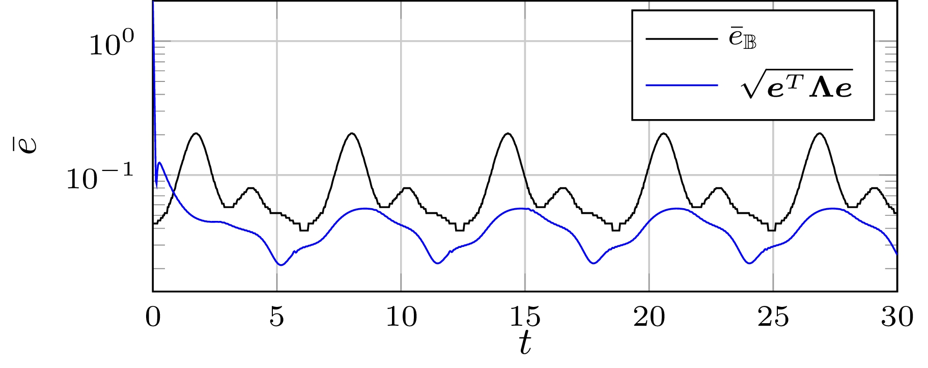
Figure 1: Radius of the ultimately bounded set (black) and tracking error observed in simulation (blue).

Snapshots of the state trajectory as well as the corresponding ultimate bound are depicted in Fig. 2. On the left hand side the maximum of the ultimate bound occurs at the maximum of $\rho\!_{\rule{0.0pt}{5.27429pt}f}(\cdot)$ along the reference trajectory. Taking a closer look at the training data, it can be seen that the training samples exhibit large control inputs $u^{(n)}$ in this area, which leads to high uncertainty in the identification of $f(\cdot)$. Therefore, there is a lack of training data, as indicated by $\rho\!_{\rule{0.0pt}{5.27429pt}f}(\cdot)$. In contrast, the right hand side of Fig. 2 shows the $\rho\!_{\rule{0.0pt}{4.82224pt}g}$-gap, which is minimal at the minimum of the ultimate bound $\bar{e}_{\mathbb{B}}$. This minimum of $\rho\!_{\rule{0.0pt}{4.82224pt}g}(\cdot)$ is a consequence of the choice of $g(\cdot)$, which is increasing with respect to $x_{2}$ in the considered state space $\mathbb{X}$. Therefore, model uncertainties have a slightly weaker effect in the upper half plane than in the lower half plane. Furthermore, it can be clearly observed that $\rho\!_{\rule{0.0pt}{4.82224pt}g}(\cdot)$ exhibits a maximum along the trajectory at $[-2\ 0]^{T}$. In fact, this lack of training data with high control inputs $u^{(n)}$ causes the second local maximum in the ultimate bound at $2\pi m+4$, $m\in\mathbb{N}$. Finally, both $\rho$-gaps show different behavior with increasing distance to the reference trajectory: Due to the increasing nominal derivative $\dot{V}_{\mathrm{nom}}(\cdot)$, $\rho\!_{\rule{0.0pt}{5.27429pt}f}(\cdot)$ is strongly decreasing, while a similar growth of the control input $\pi(\bm{x})$ compensates this effect, causing a growing $\rho\!_{\rule{0.0pt}{4.82224pt}g}(\cdot)$.

VI CONCLUSION

This paper introduces a quality measure for training sets in data-driven control. We establish a relationship between the distribution of the training data and the ultimate bound of the tracking error for a Gaussian process-based control law. In contrast to state-of-the-art information-theoretical quantities, our measure allows us to determine the most useful data points for control. In future work, this can be used to design exploration algorithms that collect data such that the control performance of the control law is maximized.

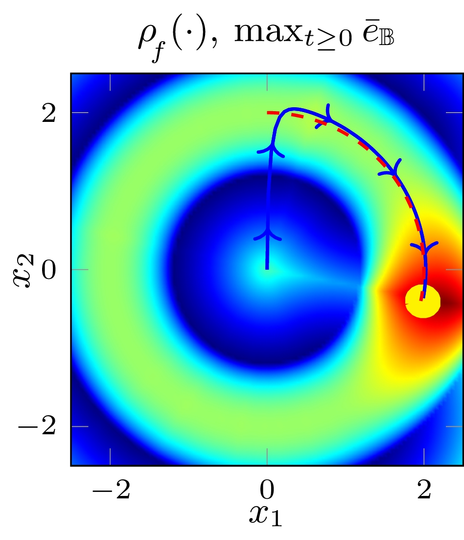
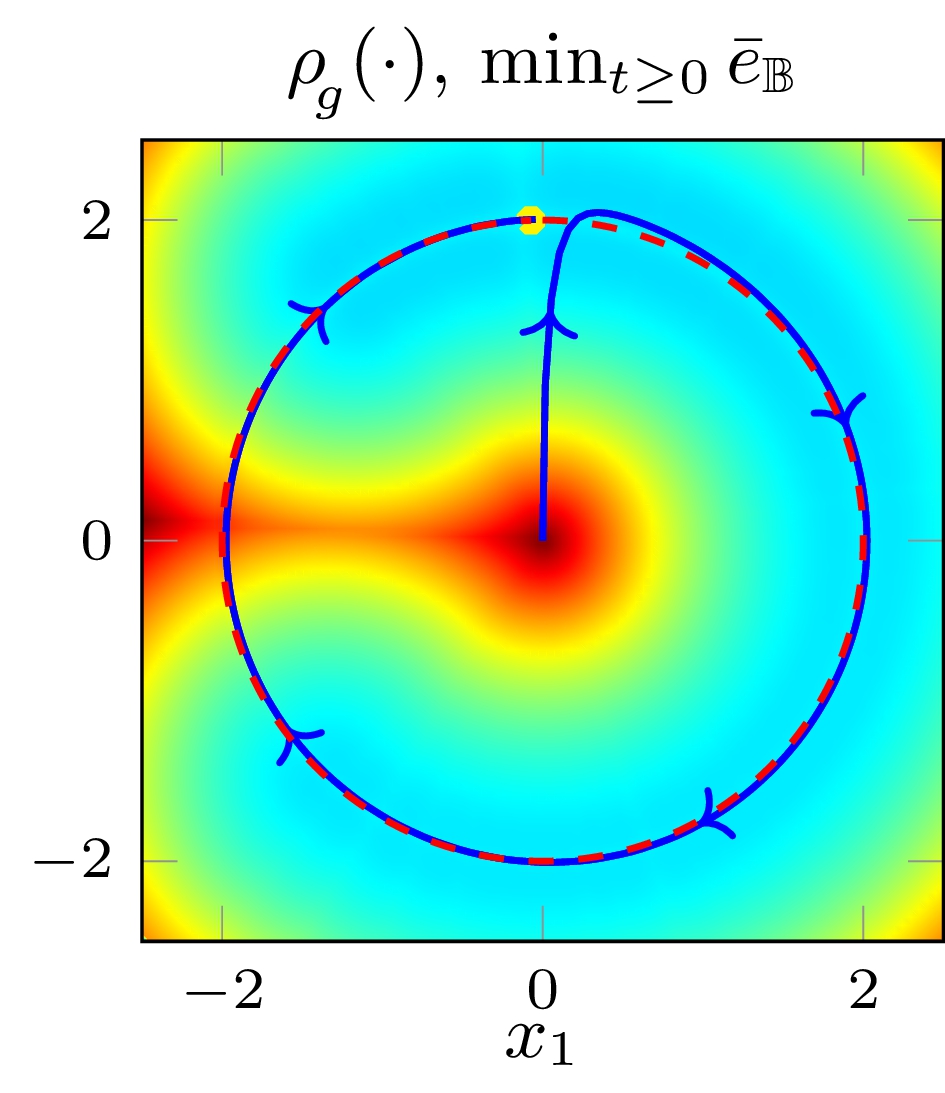
Figure 2: Snapshots of the state trajectory (blue) and reference trajectory (red) of the system controlled with $N=1000$ training samples obtained using a high gain controller. Large ultimate bounds are strongly related to large values of $\rho\!_{\rule{0.0pt}{5.27429pt}f}(\cdot)$ and $\rho\!_{\rule{0.0pt}{4.82224pt}g}(\cdot)$ (red background).

References

• [1] L. Ljung, System Identification.   NJ, USA: Prentice Hall PTR, 1998.
• [2] J. Kocijan, R. Murray-Smith, C. E. Rasmussen, and A. Girard, “Gaussian process model based predictive control,” in Proceedings of the 2004 American Control Conference, 2004, pp. 2214–2219.
• [3] J. F. Fisac, A. K. Akametalu, M. N. Zeilinger, S. Kaynama, J. Gillula, and C. J. Tomlin, “A General Safety Framework for Learning-Based Control in Uncertain Robotic Systems,” IEEE Transactions on Automatic Control, vol. 64, no. 7, pp. 2737–2752, 2019.
• [4] J. Umlauft, A. Lederer, and S. Hirche, “Learning Stable Gaussian Process State Space Models,” in Proceedings of the American Control Conference, 2017, pp. 1499–1504.
• [5] A. Lederer, J. Umlauft, and S. Hirche, “Uniform Error Bounds for Gaussian Process Regression with Application to Safe Control,” in Advances in Neural Information Processing Systems, 2019.
• [6] F. Berkenkamp, A. P. Schoellig, and A. Krause, “Safe Controller Optimization for Quadrotors with Gaussian Processes,” in Proceedings of the IEEE International Conference on Robotics and Automation, 2016, pp. 491–496.
• [7] T. Beckers, D. Kulić, and S. Hirche, “Stable Gaussian Process based Tracking Control of Euler-Lagrange Systems,” Automatica, vol. 103, no. 23, pp. 390–397, 2019.
• [8] G. Chowdhary, H. A. Kingravi, J. P. How, and P. A. Vela, “Bayesian nonparametric adaptive control using Gaussian processes,” IEEE Transactions on Neural Networks and Learning Systems, vol. 26, no. 3, pp. 537–550, 2015.
• [9] T. Koller, F. Berkenkamp, M. Turchetta, and A. Krause, “Learning-based Model Predictive Control for Safe Exploration,” in Proceedings of the IEEE Conference on Decision and Control, 2018, pp. 6059–6066.
• [10] T. Alpcan and I. Shames, “An Information-Based Learning Approach to Dual Control,” IEEE Transactions on Neural Networks and Learning Systems, vol. 26, no. 11, pp. 2736–2748, 2015.
• [11] A. Capone, A. Lederer, J. Umlauft, and S. Hirche, “Data selection for multi-task learning under dynamic constraints,” 2020. [Online]. Available: http://arxiv.org/abs/2005.03270
• [12] J. Umlauft and S. Hirche, “Feedback Linearization based on Gaussian Processes with event-triggered Online Learning,” IEEE Transactions on Automatic Control, 2020.
• [13] D. K. Duvenaud, “Automatic Model Construction with Gaussian Processes,” Ph.D. dissertation, University of Cambridge, 2014.
• [14] C. E. Rasmussen and C. K. I. Williams, Gaussian Processes for Machine Learning.   Cambridge, MA: The MIT Press, 2006.
• [15] H. Wendland, Scattered Data Approximation.   Cambridge University Press, 2004.
• [16] A. Lederer, J. Umlauft, and S. Hirche, “Posterior Variance Analysis of Gaussian Processes with Application to Average Learning Curves,” 2019. [Online]. Available: http://arxiv.org/abs/1906.01404
• [17] A. Yesildirek and F. Lewis, “Feedback linearization Using Neural Networks,” in Proceedings of the IEEE Conference on Decision and Control, 1995, pp. 2539–2544.