Cosmic analogues of classic variational problems

Several classic one-dimensional problems of variational calculus originating in non-relativistic particle mechanics have solutions that are analogues of spatially homogeneous and isotropic universes. They are ruled by an equation which is formally a Friedmann equation for a suitable cosmic fluid. These problems are revisited and their cosmic analogues are pointed out. Some correspond to the main solutions of cosmology, while others are analogous to exotic cosmologies with phantom fluids and finite future singularities.

1 Introduction

Several classic one-dimensional problems of mechanics solved with variational calculus have analogues in spatially homogeneous and isotropic (or Friedmann-Lemaître-Robertson-Walker, hereafter “FLRW”) cosmology. The analytical solutions of these problems often correspond to particularly important solutions of FLRW cosmology. One can build in the laboratory many physical systems that are analogous to curved spacetimes describing black holes or universes, using which one can study curved space quantum effects such as Hawking radiation, particle creation, or superradiance. These systems include Bose-Einstein condensates and other condensed matter systems [1, 2, 3, 4, 5, 6, 7, 8, 9, 10, 11, 12, 13, 14], fluid-dynamical systems [15, 16, 17, 18, 19, 20, 21, 22, 23, 24, 25, 26, 27], and optical systems [28, 29, 30, 31, 32] and they have originated the field of research known as analogue gravity (e.g., [33, 34, 35, 36, 37]), part of which focuses on analogues of FLRW cosmology in Bose-Einstein condensates [38, 39, 40, 41, 34, 2, 3, 4, 5, 6, 7, 10]. Cosmic analogue systems can also be created with soap bubbles [42, 43] and capillary fluid flow [44]. Less known analogues for cosmology, which involve natural systems outside of the laboratory, include glacial valley profiles [45, 46], equilibrium beach profiles [47], the freezing of bodies of water [48], and the Omori-Utsu law for the aftershocks following a main earthquake shock [49].

Let us go over the basic concepts of FLRW cosmology to fix the notations and the terminology. The Einstein equations read [50, 51, 52]

$${\cal R}_{ab}-\frac{1}{2}\,g_{ab}{\cal R}+\Lambda g_{ab}=8\pi GT_{ab}\,,$$ (1.1)

where $G$ is Newton’s constant, $g_{ab}$ is the spacetime metric, ${\cal R}_{ab}$ is the Ricci tensor, ${\cal R}={{\cal R}^{a}}_{a}$ is the Ricci scalar, $\Lambda$ is the cosmological constant, and $T_{ab}$ is the stress-energy tensor of matter.

The FLRW line element is

$$ds^{2}=-dt^{2}+a^{2}(t)\left[\frac{dr^{2}}{1-Kr^{2}}+r^{2}\left(d\theta^{2}+\sin^{2}\theta\,d\varphi^{2}\right)\right]$$ (1.2)

in comoving polar coordinates $\left(t,r,\theta,\varphi\right)$, where the curvature index $K$ can be normalized to $K=1,0,-1$ (although this is not necessary), corresponding to a universe with closed three-dimensional spatial sections, Euclidean spatial sections, or hyperbolic 3-sections, respectively [51, 50, 53, 52, 54].

The matter content of the universe causing the spacetime curvature is usually modelled by a perfect fluid with stress-energy tensor

$$T_{ab}=\left(P+\rho\right)u_{a}u_{b}+Pg_{ab}\,,$$ (1.3)

where $u^{a}$ is the four-velocity of the fluid and of comoving observers, while the energy density $\rho(t)$ and isotropic pressure $P(t)$ are related by some equation of state. Usually the latter has the barotropic form $P=P(\rho)$ and often (but not necessarily) $P=w\rho$ with $w=$ const. Formally, the cosmological constant term can be treated as a special case of a perfect fluid with effective stress-energy tensor $T_{ab}^{(\Lambda)}=-\Lambda g_{ab}/(8\pi G)$ with effective equation of state $P_{\Lambda}=-\rho_{\Lambda}=-\frac{\Lambda}{8\pi G}$.

The scale factor $a(t)$ of the FLRW metric (1.2), the energy density $\rho(t)$ and the pressure $P(t)$ obey the Einstein-Friedmann equations

$$H^{2}\equiv\left(\frac{\dot{a}}{a}\right)^{2}=\frac{8\pi G}{3}\,\rho-\frac{K}{a^{2}}\,,$$ (1.4)

$$\frac{\ddot{a}}{a}=-\,\frac{4\pi G}{3}\left(\rho+3P\right)\,,$$ (1.5)

$$\dot{\rho}+3H\left(P+\rho\right)=0\,,$$ (1.6)

where an overdot denotes differentiation with respect to the comoving time $t$ and $H(t)\equiv\dot{a}/a$ is the Hubble function [51, 50, 53, 52, 54]. Only two equations in this set are independent: given any two of them, the third one can be derived from the others. Without loss of generality, we choose the Friedmann equation (1.4) and the energy conservation equation (1.6) as independent, while the acceleration equation (1.5) follows from them.

If the cosmic fluid satisfies the barotropic equation of state $P=w\rho$ with $w=$ const., the covariant conservation equation (1.6) integrates to

$$\rho(a)=\frac{\rho_{0}}{a^{3(w+1)}}\,.$$ (1.7)

Further, if the universe is spatially flat (i.e., $K=0$), the corresponding scale factor is

$$a(t)=\frac{a_{0}}{\left|t-t_{0}\right|^{3|w+1|}}\,.$$ (1.8)

Solution methods, phase space, and analytic solutions of the Einstein-Friedmann equations are reviewed in [55, 56, 57]), while [58, 45, 59] report new results. In particular, a mathematical property of the Friedmann equation (1.4) relevant here and proved in [59] is that the graphs of all solutions of this equation are roulettes. A roulette is the locus of a point that lies on, or inside, a curve that rolls without slipping along another given curve. Special cases include the elliptical cycloid, which is the curve described by a point on an ellipse as the latter rolls on the $x$-axis. When the ellipse reduces to a circle, one reproduces the ordinary cycloid (the trajectory of a point on the rim of a bicycle wheel as the bicycle advances at constant speed on horizontal ground) and is probably the most well known roulette.

It may seem that a complete analogy between the Einstein-Friedmann equations and the physical systems that we will consider is not complete because in the latter the dynamics is described by a single differential equation (analogous to the Friedmann equation), while the universe is described by two equations of the set (1.4)-(1.6). This is not the case because the information contained in the second equation (say, the covariant conservation equation (1.6)) has already been inserted into the first one (the Friedmann equation (1.4) by using the scaling (1.7) of the perfect fluid energy density and of the curvature term with the scale factor $a$ on the right hand side of Eq. (1.4), or a similar functional dependence $\rho(a)$ that characterizes the perfect fluid (for example a non-linear equation of state). Therefore, when we refer to “the Friedmann equation” we mean Eq. (1.4) plus this extra ingredient, which makes the analogy complete. All the equations for physical and geometrical problems considered in the following have a form that already includes some familiar dependence $\rho(a)$ of the fluid energy density on the scale factor and makes it suitable for a complete analogy.

In the following we review the most celebrated textbook problems of variational calculus in one dimension, building cosmological analogies where possible.

2 Geodesics of the Euclidean plane and a not-so-trivial analogue

A simple variational problem consists of finding the geodesic curves extremizing the length between two fixed points in the Euclidean plane. The infinitesimal arc length along a curve $y(x)$ in this plane is $dl=\sqrt{dx^{2}+dy^{2}}=\sqrt{1+y^{\prime 2}}\,dx$, where $y^{\prime}\equiv dy/dx$. The finite length betwen two fixed points along this curve is the functional of the curve

$$J\left[y(x)\right]=\int_{1}^{2}dl=\int_{x_{1}}^{x_{2}}dx\,\sqrt{1+y^{\prime 2}}\equiv\int_{x_{1}}^{x_{2}}dx\,L\left(y^{\prime}(x)\right)\,.$$ (2.1)

Since the Lagrangian $L$ does not depend on $y$, the canonically conjugated momentum $\partial L/\partial y^{\prime}$ is conserved,

$$\frac{y^{\prime}}{\sqrt{1+y^{\prime 2}}}=C$$ (2.2)

or

$$y^{\prime}=\frac{C^{2}}{1-C^{2}}$$ (2.3)

which integrates trivially to $y(x)=\frac{C^{2}}{1-C^{2}}\,x+D$, giving straight lines as the geodesics of the Euclidean plane. This equation gives also

$$\left(\frac{y^{\prime}}{y}\right)^{2}=\frac{C_{1}^{2}}{y^{2}}$$ (2.4)

(where $C_{1}^{2}=C^{2}/(1-C^{2})$) and the analogous Friedmann equation (1.4) is

$$H^{2}=\frac{C_{1}^{2}}{a^{2}}\,.$$ (2.5)

It describes an empty cosmos with hyperbolic ($K=-1$) spatial sections, known as the Milne universe. This solution of the Einstein-Friedmann equations is nothing but Minkowski spacetime in disguise because of a hyperbolic foliation (i.e., in accelerated coordinates). In these coordinates, flat spacetime is sliced with negatively curved spatial sections, all the components of the Riemann tensor vanish identically, but the intrinsic curvature of the spatial 3-sections does not [60].

The function $H(a)$ is given in Fig. 1.

3 The catenary problem

Consider a heavy string hanging in a vertical $\left(x,y\right)$ plane and described by the profile $y(x)$. The linear density is $\mu=dm/dl$, where $dl=\sqrt{dx^{2}+dy^{2}}=\sqrt{1+(y^{\prime})^{2}}\,dx$ is the elementary arc length along the string. The gravitational potential energy of an element of string of length $dl$ located at horizontal position $x$ is $dE_{g}=\mu gy(x)ds$. The total gravitational potential energy of a string suspended by two points of horizontal coordinates $x_{1}$ and $x_{2}$ is the functional of the curve $y(x)$

$$E_{g}\left[y(x)\right]=\mu g\int_{x_{1}}^{x_{2}}dx\,y\sqrt{1+(y^{\prime})^{2}}\equiv\int_{x_{1}}^{x_{2}}L\,dx\,.$$ (3.1)

The Lagrangian $L\left(y(x),y^{\prime}(x)\right)$ does not depend explicitly on the coordinate $x$ and, therefore, the corresponding Hamiltonian is conserved:

$${\cal H}=\frac{\partial L}{\partial y^{\prime}}\,y^{\prime}-L=c_{1}\,,$$ (3.2)

where $c_{1}$ is a constant. Equation (3.2) (known as the Beltrami identity) simplifies to

$$\frac{-y}{\sqrt{1+(y^{\prime})^{2}}}=c_{1}\,,$$ (3.3)

which has catenaries as solutions [61].

Although not necessary, the variational principle is sometimes imposed subject to the constraint that the string length between $x_{1}$ and $x_{2}$ is fixed, which changes the variational integral to

$$J\left[y(x)\right]=\int_{x_{1}}^{x_{2}}dx\,\left(y+\lambda\right)\sqrt{1+(y^{\prime})^{2}}\,,$$ (3.4)

where $\lambda$ is a Lagrange multiplier. A shift $y\rightarrow\bar{y}\equiv y+\lambda$ reduces this problem to the previous one.

The cosmological analogue of Eq. (3.3) corresponds to a well known situation in cosmic physics. This equation is recast as

$$\left(\frac{y^{\prime}}{y}\right)^{2}=\frac{1}{C_{1}^{2}}-\frac{1}{y^{2}}\,,$$ (3.5)

the analogue of which for the scale factor $a(t)$ reads

$$H^{2}=\frac{\Lambda}{3}-\frac{1}{a^{2}}\,,$$ (3.6)

where $\Lambda=3/C_{1}^{2}>0$ is the cosmological constant. We continue the discussion in the next problem, which leads to the same cosmic analogue.

4 Minimal surface of revolution and its analogue

Another classic problem of variational calculus is that of the minimal surface of revolution. Let $y(x)$ join two points in the vertical $\left(x,y\right)$ plane and rotate this curve about the vertical (or $y$-) axis. The problem of finding the curve that achieves the surface of minimal area is solved by extremizing the area integral [61]

$$J=\int_{x_{1}}^{x_{2}}dx\,x\sqrt{1+\left(\frac{dy}{dx}\right)^{2}}\,.$$ (4.1)

A practical application is given by soap bubbles between wire frames. Since the energy of a soap bubble is proportional to its area, nature tends to minimize it and to achieve the minimal surface of revolution when soapy water is placed on a wire frame obtained by rotating about the $y$-axis a wire shaped as the graph of $y(x)$.

4.1 Dependent variable $x=x(y)$

It is now convenient to take $x(y)$ as the dependent variable instead of $y(x)$ and to rewrite the integral as

$$J\left[x(y)\right]=\int_{y_{1}}^{y_{2}}dy\,x\sqrt{1+\left(\frac{dx}{dy}\right)^{2}}\equiv\int_{y_{1}}^{y_{2}}dy\,L\left(x(y),\frac{dx}{dy}\right)\,,$$ (4.2)

where $y_{1,2}\equiv y(x_{1,2})$. Since $\partial L/\partial y=0$ the corresponding Hamiltonian is conserved,

$${\cal H}=\frac{\partial L}{\partial x^{\prime}}\,x^{\prime}-L=\frac{xx^{\prime 2}}{\sqrt{1+x^{\prime 2}}}-x\sqrt{1+x^{\prime 2}}=C\,,$$ (4.3)

where $C$ is a constant and now $x^{\prime}\equiv dx/dy$. Manipulation of this equation yields

$$x^{\prime 2}=\frac{x^{2}}{C^{2}}-1\,,$$ (4.4)

which is solved by separation of variables, leading to

$$\int\frac{dx}{\sqrt{x^{2}-C^{2}}}=\ln\left(\sqrt{x^{2}-C^{2}}+x\right)=\frac{y-y_{0}}{C}$$ (4.5)

where $y_{0}$ is an integration constant. By exponentiating both sides, a little algebra gives easily the solution

$$x(y)=\frac{1}{2}\left(\mbox{e}^{\frac{y-y_{0}}{C}}+C^{2}\mbox{e}^{-\,\frac{y-y_{0}}{C}}\right)\,.$$ (4.6)

The initial conditions $C=\pm 1$ yield the catenary curve

$$x(y)=\cosh\left(y-y_{0}\right)$$ (4.7)

and $y_{0}=\cosh^{-1}x_{0}$ where $x_{0}\equiv x(0)$.

The cosmic analogue is obtained by rewriting Eq. (4.4) as

$$\left(\frac{x^{\prime}}{x}\right)^{2}=\frac{1}{C^{2}}-\frac{1}{x^{2}}\,.$$ (4.8)

The analogous Friedmann equation (1.4) is

$$H^{2}=\frac{\Lambda}{3}-\frac{1}{a^{2}}\,,$$ (4.9)

the right hand side of which contains a contribution from the positive cosmological constant $\Lambda=3/C^{2}$ and a contribution from the curvature term $-K/a^{2}$ with $K=+1$. The analogous universe is well known as the positively curved universe with no matter and a pure (positive) cosmological constant; it evolves with scale factor

$$a(t)=\sqrt{\frac{3}{\Lambda}}\,\cosh\left[\sqrt{\frac{\Lambda}{3}}\,\left(t-t_{0}\right)\right]\,.$$ (4.10)

This catenary history of the universe includes a contracting phase (eternal in the past) for $t<t_{0}$, a bounce (made possible by the fact that the cosmological constant violates the strong energy condition and avoids the singularity) at $t=t_{0}$, followed by external expansion for $t>t_{0}$. The universe asymptotes to the de Sitter space with scale factor

$$a_{dS}(t)=\sqrt{\frac{3}{4\Lambda}}\,\exp\left[\sqrt{\frac{\Lambda}{3}}\,\left(t-t_{0}\right)\right]$$ (4.11)

as $t\rightarrow+\infty$.

4.2 Dependent variable $y=y(x)$

In this case the Lagrangian is

$$L\left(x,y^{\prime}(x)\right)=x\sqrt{1+y^{\prime 2}}\,;$$ (4.12)

since $\partial L/\partial y=0$ the canonically conjugated momentum is conserved,

$$\frac{\partial L}{\partial y^{\prime}}=\frac{xy^{\prime}}{\sqrt{1+y^{\prime 2}}}=C\,.$$ (4.13)

This equation leads to

$$y^{\prime}=\frac{C}{\sqrt{x^{2}-C^{2}}}\,,$$ (4.14)

which integrates to $y(x)=C\ln\left(\sqrt{x^{2}-C^{2}}+x\right)+\mbox{const}.$ and manipulations lead again to $x(y)=\cosh\left(y-y_{0}\right)$ if $C=\pm 1$. There is no cosmic analogue with this choice of variable because the putative analogue of the Friedmann equation

$$\frac{y^{\prime 2}}{y^{2}}=\frac{C^{2}}{y^{2}\left(x^{2}-C^{2}\right)}$$ (4.15)

contains $x$ explicitly, contrary to the Friedmann equation (1.4) that does not contain $t$ explicitly.

The function $H(a)$ is given in Fig. 1, while the scale factor $a(t)$ is reported in Fig. 2.

5 Cosmic analogue of the brachistochrone problem

The brachistocrone is the curve in the vertical plane that connects two given points (not on the same vertical) and such that a particle sliding on it without friction arrives at the bottom in the minimum time. The classic problem of finding this curve was posed to the elite mathematical community by Johann Bernoulli in 1696 [62].

The speed $v$ of a particle falling from rest ($v_{0}=0$) from the height $y$ is given by energy conservation,

$$\frac{mv^{2}}{2}=mgy$$ (5.1)

(where $g$ is the constant acceleration of gravity), from which one obtains the well known result $v=\sqrt{2gy}$. The descent time from point $1$ to point $2$ along the curve $y(x)$ with arc length $dl=\sqrt{dx^{2}+dy^{2}}$ is

$$J\left[y(x)\right]=\int_{1}^{2}dt=\int_{1}^{2}\frac{dl}{v}=\int_{x_{1}}^{x_{2}}dx\,\sqrt{\frac{1+y^{\prime 2}}{2gy}}\equiv\int_{x_{1}}^{x_{2}}dx\,L\left(y(x),y^{\prime}(x)\right)\,,$$ (5.2)

where $y(x)$ are trajectories from $1$ to $2$ in the vertical $\left(x,y\right)$ plane, and a prime denotes differentiation with respect to $x$. Clearly, it must be $y>0$. The descent time is extremized, $\delta J=0$, if $L$ satisfies the Euler-Lagrange equation.

Since $\partial L/\partial x=0$ the corresponding Hamiltonian is conserved,

$${\cal H}=\frac{\partial L}{\partial y^{\prime}}\,y^{\prime}-L=C_{0}\,,$$ (5.3)

where $C_{0}$ is a constant. This Beltrami identity can be written as

$$\sqrt{y\left(1+y^{\prime 2}\right)}=C_{1}$$ (5.4)

(with $C_{1}=-1/(C_{0}\sqrt{2g})>0$), from which one obtains

$$y^{\prime 2}=\frac{C_{1}^{2}}{y}-1\,,$$ (5.5)

which has a cycloid (the prototypical roulette) as its well known solution [61]. One can divide both sides of Eq. (5.5) by $y^{2}$ to obtain

$$\left(\frac{y^{\prime}}{y}\right)^{2}=\frac{C_{1}^{2}}{y^{3}}-\frac{1}{y^{2}}\,,$$ (5.6)

which is analogous to the Friedmann equation

$$H^{2}=\frac{8\pi G\rho_{0}}{3a^{3}}-\frac{1}{a^{2}}$$ (5.7)

describing a closed ($K=+1$) FLRW universe filled with a fluid with equation of state parameter $w=0$, i.e., a dust with energy density scaling as $\rho=\rho_{0}/a^{3}$. It is significant that the energy density comes out positive, which could spoil the analogy if it wasn’t true and is not to be taken for granted when building analogies. This is a very simple matter-dominated universe and a classic textbook case. The solution is expressed in parametric form by

$$a(\eta) = \frac{C_{2}}{2}\left(1-\cos\eta\right)\,,$$ (5.8)

$$t(\eta) = \frac{C_{2}}{2}\left(\eta-\sin\eta\right)\,,$$ (5.9)

where the parameter $\eta$ is the conformal time, the initial condition $a(t=0)=0$ has been imposed, and $C_{2}=8\pi G\rho_{0}$.

On the mechanical side of the analogy, the parameter $\eta$ (the analog of conformal time) is defined by $dx=yd\eta$, which means that small increments of $\eta$ are small increments of the coordinate $x$ measured in units of the height of the point lying on the brachistrochrone curve.

Equation (5.5) shows that $y^{\prime}\rightarrow\infty$ as $y\rightarrow 0$: the curve must start vertical, with a cusp, at its highest point. On the cosmology side of the analogy, this peculiarity corresponds to the fact that a universe filled with dust and positively curved necessarily begins at a Big Bang singularity; this is a special case of the general Hawking-Penrose singularity theorems satisfied by matter obeying the null energy condition (in this case, dust satisfies also the strong, weak, and dominant energy conditions [50]).

The function $H(a)$ is given in Fig. 1, while the scale factor $a(t)$ is reported in Fig. 3.

6 Geodesics of the Poincaré half-plane

The Poincaré half-plane is the upper part of the $\left(x,y\right)$ plane with $y>0$ and the metric given by the line element

$$ds^{2}=\frac{1}{y^{2}}\left(dx^{2}+dy^{2}\right)$$ (6.1)

conformal to the Euclidean metric. The arc length along a curve $y(x)$ is $dl=\sqrt{dx^{2}+dy^{2}}/y$ and geodesics are found by extremizing the finite length

$$l\left[y(x)\right]=\int_{x_{1}}^{x_{2}}dx\,\frac{\sqrt{1+y^{\prime 2}}}{y}\equiv\int_{x_{1}}^{x_{2}}dx\,L\left(y,y^{\prime}\right)$$ (6.2)

between two given points. Since $\partial L/\partial x=0$ the corresponding Hamiltonian is conserved,

$$\frac{\partial L}{\partial y^{\prime}}\,y^{\prime}-L=C<0\,,$$ (6.3)

which yields

$$\frac{1}{Cy}=-\sqrt{1+y^{\prime 2}}\,.$$ (6.4)

The solutions for $C=-1$ are half-circles perpendicular to the $x$-axis.

The cosmic analogue obtained from Eq. (6.4)

$$H^{2}=\frac{1}{C^{2}a^{4}}-\frac{1}{a^{2}}$$ (6.5)

describes a positively curved ($K=+1$) universe filled with a radiation fluid with equation of state $P=\rho/3$ and $\rho=\rho_{0}/a^{4}$, $\rho_{0}=\frac{3}{8\pi GC^{2}}$. This is another classic textbook example with scale factor

$$a(t)=\sqrt{C^{\prime}}\sqrt{1-\left(1-\frac{t}{C^{\prime}}\right)^{2}}\,,$$ (6.6)

where $C^{\prime}=1/C^{2}$. This analogy was already discussed in Rindler’s textbook [63] and in Ref. [42].

The function $H(a)$ is given in Fig. 1, while the scale factor $a(t)$ is reported in Fig. 2.

7 The gravity tunnel

A popular problem in introductory physics courses consists of analyzing the motion of a particle through a tunnel dug out along a diameter of the Earth, which is modelled as a uniform sphere [64, 65, 66, 67, 68, 69] (see [70] for a non-uniform sphere). A homogeneous sphere of mass $M$ and radius $R$ has density $\rho_{s}=\frac{3M}{4\pi R^{3}}$ and the spherically symmetric Newtonian potential $\Phi(r)$ satisfies the Poisson equation

$$\frac{1}{r^{2}}\,\frac{d}{dr}\left(r^{2}\,\frac{d\Phi}{dr}\right)=4\pi G\rho_{s}$$ (7.1)

inside the sphere. This readily integrates to

$$\Phi(r)=\frac{GM}{2R^{3}}\,r^{2}-\frac{C_{1}}{r}+C_{2}\,,$$ (7.2)

where $C_{1,2}$ are integration constants. Regularity at the centre requires $C_{1}=0$ and matching the exterior potential $\Phi_{out}=-GM/r$ at the surface $r=R$ yields $C_{2}=-\,\frac{3GM}{2R}$. Therefore, the potential inside the homogeneous sphere

$$\Phi(r)=\frac{GM}{2R^{3}}\,r^{2}-\frac{3GM}{2R}$$ (7.3)

is that of a shifted harmonic oscillator and the particle oscillates up and down the tunnel.

The Lagrangian for a particle of mass $m$ and position $r(t)$ moving without friction through this gravity tunnel is

$$L\left(r,\dot{r}\right)=\frac{m\dot{r}^{2}}{2}-\frac{GM}{2R^{3}}\,r^{2}+\frac{3GM}{2R}\,;$$ (7.4)

since $\partial L/\partial t=0$ the corresponding Hamiltonian (which coincides with the particle energy) is conserved,

$$\frac{\partial L}{\partial\dot{r}}\,\dot{r}-L=E\,,$$ (7.5)

expressing the energy integral

$$\frac{m\dot{r}^{2}}{2}+m\left(\frac{GM}{2R^{3}}\,r^{2}-\frac{3GM}{2R}\right)=E\,.$$ (7.6)

This Beltrami identity can be rearranged as

$$\left(\frac{\dot{r}}{r}\right)^{2}=-\frac{GM}{R^{3}}-\frac{K}{r^{2}}\,,$$ (7.7)

where $K=-\,\frac{2}{m}\left(E+\frac{3GM}{R}\right)$. The analogous Friedmann equation (1.4) for $a(t)\leftrightarrow r(t)$ is

$$H^{2}=\frac{\Lambda}{3}-\frac{K}{a^{2}}$$ (7.8)

and it exhibits a negative cosmological constant $\Lambda=-3GM/R^{3}$. There is no matter fluid in this analogous universe. Since $H^{2}\geq 0$, only a negative negative curvature index $K<0$ is possible to compensate for the negative $\Lambda$. Apart from the dimensionality, this universe is the anti-de Sitter spacetime of the AdS/CFT correspondence and the holographic principle [71]. The solution of Eq. (7.8) is the scale factor

$$a(t)=\sqrt{\frac{3}{|\Lambda|}}\,\sin\left(\sqrt{\frac{|\Lambda|}{3}}\,t\right)\,.$$ (7.9)

The function $H(a)$ is given in Fig. 1, while the scale factor $a(t)$ is reported in Fig. 2.

8 The terrestrial brachistochrone

In the terrestrial brachistochrone problem [65, 67], tunnels of various curved shape described by functions $r(\theta)$ in polar coordinates, are dug out in the uniform Earth of radius $R$, and one looks for the shape that minimizes the transit time between two given points. This problem has seen much renewed attention recently, mostly in the pedagogical literature [72, 73, 74, 75, 76, 77, 78, 79, 80, 81, 83, 84, 85, 86] but not only [87, 88, 89].

The corresponding Lagrangian is [67]

$$L\left(r,r^{\prime}\right)=\sqrt{\frac{r^{2}+r^{\prime 2}}{R^{2}-r^{2}}}\,,$$ (8.1)

where $r^{\prime}\equiv dr/d\theta$. Since the Lagrangian does not depend explicitly on $\theta$ the corresponding Hamiltonian is conserved,

$${\cal H}=\frac{\partial L}{\partial r^{\prime}}\,r^{\prime}-L=C\,,$$ (8.2)

leading to

$$\frac{r^{2}}{\sqrt{R^{2}-r^{2}}\,\sqrt{r^{2}+r^{\prime 2}}}=-C\,.$$ (8.3)

Further manipulation gives

$$\frac{r^{\prime 2}}{r^{2}}=-1+\frac{r^{2}}{C^{2}\left(R^{2}-r^{2}\right)}\,.$$ (8.4)

The minimum radius is attained where the curve $r(\theta)$ flattens, $r^{\prime}=0$, yielding

$$C^{2}=\frac{r_{\text{min}}^{2}}{R^{2}-r_{\text{min}}^{2}}\,,$$ (8.5)

then one can write

$$\frac{r^{2}+r^{\prime 2}}{r^{2}}=\frac{r^{2}}{r_{\text{min}}^{2}}\,\frac{(R^{2}-r_{\text{min}}^{2})}{R^{2}-r^{2}}\,.$$ (8.6)

The analogous Friedmann equation

$$H^{2}=-1+\frac{a^{2}}{C^{2}\left(a_{0}^{2}-a^{2}\right)}$$ (8.7)

is more interesting than in the situations discussed previously. The universe contains a negative cosmological constant $\Lambda=-3$ and a perfect fluid with energy density

$$\rho=\rho_{0}\,\frac{a^{2}}{a_{0}^{2}-a^{2}}\,,\;\;\;\;\;\;\;\;\frac{8\pi G}{3}\,\rho_{0}=\frac{1}{C^{2}}\,.$$ (8.8)

By imposing the covariant conservation equation $\dot{\rho}+3H(P+\rho)=0$, one finds the equation of state of the cosmic fluid. First, we obtain

$$P=-\rho-\frac{2\rho_{0}a_{0}^{2}\,a^{2}}{3\left(a_{0}^{2}-a^{2}\right)^{2}}\,;$$ (8.9)

then, using $\frac{a^{2}}{(a_{0}^{2}-a^{2})^{2}}=\left(\frac{\rho}{\rho_{0}}\right)^{2}\frac{1}{a^{2}}$ and $a^{2}=\frac{\rho}{\rho_{0}}\,\frac{a_{0}^{2}}{(1+\rho/\rho_{0})}$, one derives the quadratic barotropic equation of state

$$P(\rho)=-\frac{5}{3}\,\rho-\frac{2}{3}\frac{\rho^{2}}{\rho_{0}}\,.$$ (8.10)

Since $P<-\rho$ this equation describes a phantom fluid [90]. Equations of state of the cosmic fluid with the form $P=\sum_{k=1}^{m}c_{k}\rho_{(k)}^{k}$ have been studied recently in cosmology [45, 59, 91] as forms of dark energy. In particular, quadratic equations of state are the subject of several works [92, 93, 94, 95, 96, 97]. These exotic equations of state produce peculiar types of spacetime singularities. While traditional cosmological solutions for linear barotropic equations of state contain Big Bang, Big Crunch, and Big Rip type singularities, the discovery of the acceleration of the universe in 1998 prompted the consideration of many more exotic non-linear equations of state for the dark energy fluid, which must be postulated in order to explain the cosmic acceleration within general relativity. This broadening of the picture results in a much wider spectrum of possible singularities [98, 99, 100, 101, 102, 103, 104, 91, 105, 106].

The Ricci scalar

$${\cal R}=-\rho_{total}+3P_{total}=\frac{1}{2\pi G}-6\rho-2\,\frac{\rho^{2}}{\rho_{0}}$$ (8.11)

diverges as $a\rightarrow a_{0}$, signalling a spacetime singularity where the scale factor stays finite but $H,\rho$, and $P$ diverge. In the mechanical side of the analogy, $a_{0}$ corresponds to $R$, the boundary of the physical problem. On the cosmology side of the analogy, $a_{0}$ is a barrier that cannot be crossed dynamically: $a(t)$ always remains smaller than $a_{0}$, but it approaches it, as will soon be clear. The graph of $a(t)$ has a cusp where $a$ reaches $a_{0}$, as is evident from the Friedmann equation (8.7). In the analogy, this feature corresponds to the fact that the terrestrial brachistochrone starts at the surface ($r=R$, corresponding to $a=a_{0}$) perpendicular to it with infinite derivative $r^{\prime}\equiv dr/d\theta$ [67, 70].

The fact that there is a minimum value of $a(t)$ also follows immediately from Eq. (8.7). Since it must be $H^{2}\geq 0$, the region $a<a_{\text{min}}$ is forbidden to the dynamics, where

$$a_{\text{min}}^{2}=\frac{C^{2}a_{0}^{2}}{1+C^{2}}\,,$$ (8.12)

is the value of $a$ corresponding to $H=0$; therefore the dynamics is restricted to the strip of the $\left(t,a\right)$ plane

$$a_{\text{min}}\leq a(t)<a_{0}\,.$$ (8.13)

We also have

$$C^{2}=\frac{3}{8\pi G\rho_{0}}=\frac{a_{\text{min}}^{2}}{a_{0}^{2}-a_{\text{min}}^{2}}\,.$$ (8.14)

This minimum value of $a$ is the analogue of the minimum radius $r_{\text{min}}$ that can be reached, but not passed, by a particle in motion on the terrestrial brachistochrone (this curve does not pass through the centre of the Earth) [67, 70].

The static universe with $a(t)\equiv a_{\text{min}}$ is an exact solution of the Einstein-Friedmann equations, corresponding to a balance between $\Lambda<0$ (which is attractive) and $(\rho+3P)<0$, which is repulsive in the acceleration equation (1.5), where these terms appear with opposite sign and compete. Since this equilibrium is fine-tuned, one expects the static solution to be unstable. Indeed, a linear perturbation analysis reveals an exponentially growing mode (see the Appendix). This static solution is the only fixed point of the dynamics and is unstable and a repellor.

Further, the acceleration equation (1.5) gives $\ddot{a}>0$ for all values of the scale factor $a_{\text{min}}<a(t)<a_{0}$; the concavity of $a(t)$ faces upward, its derivative $\dot{a}$ increases, and is larger and larger the closer the orbit of the solution gets to the singularity $a_{0}$. The picture of the dynamics that emerges from these considerations is the following: solutions starting anywhere in the strip $a_{\text{min}}<a<a_{0}$ move toward the singularity faster and faster, with increasing “speed” $\dot{a}$, until they hit it and the universe ends in a finite proper time, with this finite value $a_{0}$ of the scale factor.

The analogy that we have created provides an explicit example of a universe dominated by a phantom fluid with quadratic equation of state. This analogy is useful since the exact solution of the terrestrial brachistochrone is known [67, 70]. It is a hypocycloid, the curve generated by a circle of radius $\left(R-r_{\text{min}}\right)/2$ rolling without sliding at constant speed inside the larger circle of radius $R$ (clearly, this curve is another roulette). It can be given in parametric form as

$$r^{2}(t) = \frac{R^{2}+r_{\text{min}}^{2}}{2}-\frac{\left(R^{2}-r_{\text{min}}^{2}\right)}{2}\,\cos\left(2\omega\,t\right)\,,$$ (8.15)

$$\theta(t) = \tan^{-1}\left[\frac{R}{r_{\text{min}}}\,\tan(\omega\,t)\right]-\frac{r_{\text{min}}}{R}\,\omega\,t\,,$$ (8.16)

where time is the parameter, $\omega=2\pi/T$, and

$$T=\pi\sqrt{\frac{R^{2}-r_{\text{min}}^{2}}{Rg}}$$ (8.17)

(with $g$ the acceleration of gravity at the surface) is the travel time between two points on the surface of the Earth, which is the minimum travel time among all tunnel configurations between these two points [67, 70]. The solution can be written also as [67, 70]

$$\theta(r) = \tan^{-1}\left(\frac{R}{r_{\text{min}}}\,\sqrt{\frac{r^{2}-r_{\text{min}}^{2}}{R^{2}-r^{2}}}\right)-\frac{r_{\text{min}}}{R}\,\tan^{-1}\left(\sqrt{\frac{r^{2}-r_{\text{min}}^{2}}{R^{2}-r^{2}}}\,\right)\,,$$ (8.18)

$$t(r) = \frac{\sqrt{R^{2}-r_{\text{min}}^{2}}}{2\sqrt{Rg}}\,\cos^{-1}\left(\frac{R^{2}+r_{\text{min}}^{2}-2r^{2}}{R^{2}-r_{\text{min}}^{2}}\right)\,.$$ (8.19)

The exact solution can immediately be transposed into the solution for the analogous universe

$$a^{2}(s) = \frac{a_{0}^{2}+a_{\text{min}}^{2}}{2}-\frac{\left(a_{0}^{2}-a_{\text{min}}^{2}\right)}{2}\cos\left(2\omega\,s\right)\,,$$ (8.20)

$$t(s) = \tan^{-1}\left[\frac{a_{0}}{a_{\text{min}}}\,\tan(\omega\,s)\right]-\frac{a_{\text{min}}}{a_{0}}\,\omega\,s\,,$$ (8.21)

or

$$t(a) = \tan^{-1}\left(\frac{a_{0}}{a_{\text{min}}}\,\sqrt{\frac{a^{2}-a_{\text{min}}^{2}}{a_{0}^{2}-a^{2}}}\right)-\frac{a_{\text{min}}}{a_{0}}\,\tan^{-1}\left(\sqrt{\frac{a^{2}-a_{\text{min}}^{2}}{a_{0}^{2}-a^{2}}}\,\right)\,,$$ (8.22)

$$s(a) = \frac{\sqrt{a_{0}^{2}-a_{\text{min}}^{2}}}{2\sqrt{a_{0}g}}\,\cos^{-1}\left(\frac{a_{0}^{2}+a_{\text{min}}^{2}-2a^{2}}{a_{0}^{2}-a_{\text{min}}^{2}}\right)\,.$$ (8.23)

The singularity $a=a_{0}$ is approached, and the universe ends its existence, in a finite time. In fact, the limit $a\rightarrow a_{0}$ in the parametric solution (8.20), (8.21) yields the parameter value $s_{0}=\pi\,\sqrt{\frac{a_{0}^{2}-a_{\text{min}}^{2}}{a_{0}g}}$ and the finite time

$$t_{0}=\frac{\pi}{2}\left(1-\frac{a_{\text{min}}}{a_{0}}\right)\,.$$ (8.24)

By equating $t_{0}$ with $T/2$, we obtain

$$g=a_{0}\left(\frac{a_{0}+a_{\text{min}}}{a_{0}-a_{\text{min}}}\right)$$ (8.25)

in the cosmic analogue.

The function $H(a)$ is given in Fig. 1, while the scale factor $a(t)$ is reported in Fig. 3.

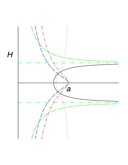
Figure 1: The functions $H(a)$ for the problems discussed. The curves correspond, respectively, to the catenary/minimal surface of revolution problems (black, solid); the brachistochrone problem (blue, dashed); the problem of the Poincaré half plane geodesics (red, dash-dotted); the gravity tunnel problem for $K=-1,0$ (green, long-dashed) or $K=1$ (black, solid); and the terrestrial brachistochrone problem (chocolate, dotted).

Figure 2: The scale factor $a(t)$ for the problems discussed. The curves correspond, respectively, to the catenary/minimal surface of revolution problems (black, solid); the Poincaré half plane geodesics problem (blue, dashed); and the gravity tunnel problem (red, dash-dotted).

Figure 3: The scale factor $a(t)$ for the remaining problems discussed. The curves correspond, respectively, to the brachistochrone problem (black, solid) and the terrestrial brachistochrone problem (blue, dashed).

9 Discussion and conclusions

Several classic problems of variational calculus originating in one-dimensional non-relativistic particle mechanics have solutions that constitute analogues of spatially homogeneous and isotropic universes because they are ruled by an equation which is formally a Friedmann equation for a suitable perfect fluid. This property suggest that it is possible to build mechanical analogues of cosmological spacetimes. If one begins with a universe with a given curvature index $K$ and equation of state $P=w(a)\rho$, the Friedmann equation (1.4) looks like an energy conservation equation and immediately suggests the point-like Hamiltonian

$${\cal H}=\frac{\dot{a}^{2}}{2}-\frac{4\pi G}{3}\,\rho a^{2}$$ (9.1)

(which is constant and equal to $-K/2$) and the point-like Lagrangian

$$L\left(a,\dot{a}\right)=\frac{\dot{a}^{2}}{2}+\frac{4\pi G}{3}\,\rho a^{2}\,.$$ (9.2)

One can then compare this Lagrangian and Hamiltonian with that of an (otherwise unrelated) mechanical or geometrical system, as we have mostly done throughout this manuscript. Alternatively, one can compare directly a first order integral for the system with the Friedmann equation (1.4), or compare the second order equation of motion with the acceleration equation (1.5).

We make no claim that the analogies proposed are full physical analogies. They may be limited to the mathematics, i.e., formal analogies, as in the classic analogy between (forced and damped) mechanical oscillators and RLC electric circuits reported in [61] and in most mechanics textbooks. There, the analogy between the equations governing the two systems is mathematical but, the equations being the same, they also have the same oscillatory solutions. This is a mathematical analogy and the two systems are completely different from the physical point of view. However, if one thinks about oscillations in nature in a general sense, the analogy has also a physical aspect. This is a physical analogy only on an abstract level and we won’t go as far as claiming it is a full physical analogy (which would bring us into semantics).

We have examined several situations: while most of them give rise to simple, albeit very important, FLRW solutions corresponding to simple fluids such as dust or radiation or a pure cosmological constant $\Lambda$, others correspond to phantom fluids [90] with non-linear equations of state originating exotic singularities at finite time, where the scale factor remains finite while curvature invariants blow up. These types of singularities are studied and classified in recent literature [98, 99, 100, 101, 102, 103, 104, 91, 105, 106]. The situations examined are summarized in Table 1.

Variational problem	Lagrangian	Cosmic analogue
Geodesics of $\mathbb{R}^{2}$	$L=\sqrt{1+y^{\prime 2}}$	$K<0,\rho=0$
		Milne universe
Catenary problem	$L=y\sqrt{1+y^{\prime 2}}$	$\Lambda>0,K>0,\rho=0$
Minimal surface of revolution	$L=x\sqrt{1+x^{\prime 2}}$	same as above
	$L=x\sqrt{1+y^{\prime 2}}$	no cosmic analogue
Brachistochrone	$L=\sqrt{\frac{1+y^{\prime 2}}{y}}$	$K>0$, dust
		cycloid
Geodesics of Poincaré plane	$L=\frac{\sqrt{1+y^{\prime 2}}}{y}$	$K>0$, radiation
Terrestrial tunnel	$L=\dot{r}^{2}-\frac{GM}{R^{3}}\,r^{2}+\frac{3GM}{R}$	$\Lambda<0,K<0,\rho=0$
		anti-de Sitter space
Terrestrial brachistochrone	$L=\sqrt{\frac{r^{2}+r^{\prime 2}}{R^{2}-r^{2}}}$	$\Lambda<0,K=0,P=-\frac{5\rho}{3}-\frac{2\rho^{2}}{3\rho_{0}}$
		hypocycloid

Table 1: Cosmic analogues of variational problems

Some of the variational problems that we have examined are centuries old and are textbook material. It is not surprising that formal analogies with the Friedmann equation (1.4) arise, since the latter takes the form of the first integral of motion corresponding to energy conservation for a particle in one-dimensional motion, and a variety of solutions are possible corresponding to the three possible curvatures and the wide range of perfect fluid equations of state (even limiting oneself to the barotropic equation $P=w\rho$ with $w=$ const.). Indeed, it is always possible to construct an analogy between a FLRW space filled by perfect fluids and the one-dimensional motion of a particle of unit mass and position $a(t)$ in a suitable potential [107], but the latter may be contrived and not physically meaningful.

Cosmic analogues have been reported for fluids [15, 16, 17, 18, 19, 20, 21, 22, 23, 24, 25, 26, 27], Bose-Einstein condensates [38, 39, 40, 41, 34, 2, 3, 4, 5, 6, 7, 10], glacial valleys [45, 46], optics [28, 29, 30, 31, 32, 45], capillary fluid flow [44], soap bubbles [42, 43], equilibrium beach profiles [47], the freezing of bodies of water [48], Omori’s law for the aftershocks following a main earthquake shock [49], etc. It is rather surprising, however, that formal analogies of classic textbook variational problems with FLRW cosmology which, as seen above, are associated with important solutions of the Friedmann equation (1.4), are not reported in the literature (with the exception of the Poincaré half-space in [63, 42]).

From the previous analysis it is clear that one-dimensional variational problems described by a Lagrangian $L\left(y(x),y^{\prime}(x)\right)$ not depending explicitly on the independent variable $x$ can have a cosmic analogue, with the Friedmann equation (1.4) corresponding to the conservation of the Hamiltonian ${\cal H}=\frac{\partial L}{\partial y^{\prime}}\,y^{\prime}-L$. However, for the cosmic analogy to begin making sense, the corresponding perfect fluid must have a non-negative energy density $\rho$, which cannot be taken for granted and dooms many would-be analogies (for all the situations discussed in this work, it is $\rho\geq 0$). Moreover, since all the solutions of the Friedmann equations are roulettes [59], only variational problems that have roulette solutions can give rise to a cosmic analogy. This fact seems to restrict considerably the range of possible solutions to the problem of building a cosmic analogue for a given one-dimensional mechanical system, and makes the existing analogies more valuable. Indeed, in our search for cosmic analogues we have encountered cycloids, hypocycloids, and catenaries, which are classic examples of roulettes.

In certain cases when $\partial L/\partial x\neq 0$, it is still possible to switch the dependent and independent variables from $y(x)$ to $x(y)$ in the action integral (and, correspondingly, change the integration variable), thus changing its form, and obtain a meaningful cosmic analogy. In general, when both descriptions admit cosmic analogues, switching dependent and independent variables leads to inequivalent cosmologies (this is not always the case, for example the problem of geodesics in the Euclidean plane leads to the same Milne universe in both descriptions, due to the simplicity of the Lagrangian $L=\sqrt{1+y^{\prime 2}}$).

The problem of the terrestrial brachistochrone, which has seen renewed attention recently [70, 72, 73, 74, 75, 76, 77, 78, 79, 80, 81, 83, 84, 85, 86, 87, 88, 89], provides an explicit example of a universe dominated by a phantom fluid with non-linear equation of state, which can be solved explicitly and exhibits a finite future singularity at a finite value of the scale factor, where the Hubble function, Ricci scalar, energy density, and pressure all diverge. Finite time singularities have been the subject of much literature in the past decade [98, 99, 100, 101, 102, 103, 104, 91, 105, 106] hence, in this problem, the mechanical side of the analogy helps the cosmology side in the sense that the known exact solution for the terrestrial brachistochrone problem can be immediately translated into an analytical solution of the corresponding cosmology with complicated (non-linear) equation of state.

These cosmological analogies are sometimes useful (this was the case for the analogy between equilibrium beach profiles, which generated solutions unknown to the oceanography community [47]; other times they are not) and they stimulate the imagination, which in the end may turn out to be their most valuable feature.

The further search for one-dimensional roulette analogues of FLRW cosmologies and the study of their small fluctuations (possibly mimicking cosmological perturbation theory) will be pursued in the future.

Appendix A Appendix: Instability of the static universe analogous to the terrestrial brachistochrone

Perturb the static universe solution so that $a(t)=a_{\text{min}}+\delta a(t)$ with $\delta a\geq 0$ since it can only be $a_{\text{min}}\leq a(t)<a_{0}$. The acceleration equation (1.5) yields

$$1-\frac{4\pi G}{3}\left(\rho_{\text{min}}+3P_{\text{min}}\right)=0$$ (A.1)

to zero order (where $\rho_{\text{min}}$ and $P_{\text{min}}$ are the energy density and pressure corresponding to $a=a_{\text{min}}$). In general, Eq. (1.5) can be written as

$$\ddot{a}=\frac{a^{3}\left(2a_{0}^{2}-a^{2}\right)}{C^{2}\left(a_{0}^{2}-a_{\text{min}}^{2}\right)^{2}}+a\,.$$ (A.2)

Expanding to first order in $\delta a/a_{\text{min}}\ll 1$, using Eq. (8.14), and keeping only the zero order and the linear terms, one obtains

$$\delta\ddot{a}\simeq\frac{C^{2}}{a_{\text{min}}}\left\{2a_{0}^{2}-a_{\text{min}}^{2}+\left[\frac{2C^{2}}{a_{\text{min}}}\left(2a_{0}^{2}-a_{\text{min}}^{2}+1\right)+\frac{1}{a_{\text{min}}}+1\right]\delta a\right\}+a_{\text{min}}\,.$$ (A.3)

Using the zero order equation (A.1), one obtains the equation satisfied by the perturbations $\delta a$ to first order

$$\delta\ddot{a}=\Omega^{2}\,\delta a\,,$$ (A.4)

where

$$\Omega^{2}=1+\frac{C^{2}}{a_{\text{min}}^{2}}\left[2C^{2}\left(1+2a_{0}^{2}-a_{\text{min}}^{2}\right)+1\right]$$ (A.5)

is positive because $a_{0}>a_{\text{min}}$. Therefore, the solution to linear order is

$$\delta a(t)=A\,\mbox{e}^{\Omega\,t}+B\,\mbox{e}^{-\Omega\,t}$$ (A.6)

with $\Omega\in\mathbb{R}$ and it contains a mode that diverges as time progresses. The static solution $a=a_{\text{min}}$ is unstable.

References

- [1] Barcelo, C.; Liberati, S.; Visser, M. Analog gravity from Bose-Einstein condensates. Class. Quantum Grav. 2001, 18, 1137. DOI: 10.1088/0264-9381/18/6/312
- [2] Fedichev, P.O.; Fischer, U.R. Gibbons-Hawking Effect in the Sonic de Sitter Space-Time of an Expanding Bose-Einstein-Condensed Gas. Phys. Rev. Lett. 2003 91, 240407. DOI: 10.1103/PhysRevLett.91.240407. Erratum, Phys. Rev. Lett. 2004 92, 049901(E). DOI:https://doi.org/10.1103/PhysRevLett.91.240407
- [3] Barceló, C.; Liberati, S.; Visser, M. Analog models for FRW cosmologies, Int. J. Mod. Phys. D 2003 12, 1641. DOI: 10.1142/S0218271803004092
- [4] Fedichev, P.O.; Fischer, U.R. “Cosmological” quasiparticle production in harmonically trapped superfluid gases. Phys. Rev. A 2004 69, 033602. DOI: 10.1103/PhysRevA.69.033602
- [5] Fischer, U.R.; Schützhold, R. Quantum simulation of cosmic inflation in two-component Bose-Einstein condensates. Phys. Rev. A 2004, 70, 063615. DOI: 10.1103/PhysRevA.70.063615
- [6] Chä, S.-Y.; Fischer, U.R. Probing the Scale Invariance of the Inflationary Power Spectrum in Expanding Quasi-Two-Dimensional Dipolar Condensates. Phys. Rev. Lett. 2017, 118, 130404. DOI: 10.1103/PhysRevLett.118.130404. Erratum Phys. Rev. Lett. 2017, 118, 179901(E). DOI:https://doi.org/10.1103/PhysRevLett.118.179901
- [7] Eckel, S.; Kumar, A.; Jacobson, T.; Spielman, I.B.; Campbell, G.K. A Rapidly Expanding Bose-Einstein Condensate: An Expanding Universe in the Lab. Phys. Rev. X 2018, 8, 021021. DOI:https://doi.org/10.1103/PhysRevX.8.021021
- [8] Fedichev, P.O.; Fischer, U.R. Observer dependence for the phonon content of the sound field living on the effective curved space-time background of a Bose-Einstein condensate. Phys. Rev. D 2004, 69, 064021. DOI: 10.1103/PhysRevD.69.064021
- [9] Volovik, G.E. Induced gravity in superfluid 3He. J. Low Temp. Phys. 1997, 113, 667–680. https://doi.org/10.1023/A:1022545226102
- [10] Jacobson, T.A.; Volovik, G.E. Effective spacetime and Hawking radiation from moving domain wall in thin film of 3He-A. J. Exp. Theor. Phys. Lett. 1998 68, 874–880. DOI: 10.1134/1.567808
- [11] Volovik, G.E. Links between gravity and dynamics of quantum liquids. Grav. Cosmol. 2000 6, 187–203.
- [12] Volovik, G.E. Effective gravity and quantum vacuum in superfluids, in Novello, M.; Visser, M.; Volovik, G. (eds.), Artificial Black Holes. World Scientific, Singapore, 2002, pp. 127–177.
- [13] Volovik, G.E. Black-hole horizon and metric singularity at the brane separating two sliding superfluids. J. Exp. Theor. Phys. Lett. 2002 76, 296–300. DOIhttps://doi.org/10.1134/1.1520613
- [14] Pashaev, O.K.; Lee, J.-H. Resonance Solitons as Black Holes in Madelung Fluid. Mod. Phys. Lett. A 2002, 17, 1601–1619. DOI: 10.1142/S0217732302007995
- [15] Unruh, W.G. Experimental Black-Hole Evaporation? Phys. Rev. Lett. 1981, 46, 1351–1353. DOI:https://doi.org/10.1103/PhysRevLett.46.1351
- [16] Unruh, W.G. Sonic analog of black holes and the effects of high frequencies on black hole evaporation. Phys. Rev. D 1995, 51, 2827–2838.
- [17] Visser, M. Acoustic black holes: Horizons, ergospheres, and Hawking radiation. Class. Quantum Grav. 1998, 15, 1767–1791. DOI: 10.1088/0264-9381/15/6/024
- [18] Garay, L.J.; Anglin, J.R.; Cirac, J.I.; Zoller, P. Sonic Analog of Gravitational Black Holes in Bose-Einstein Condensates. Phys. Rev. Lett. M2000, 85, 4643-4647. DOI: 10.1103/PhysRevLett.85.4643
- [19] Fischer, U.R.; Visser, M. Riemannian geometry of irrotational vortex acoustics. Phys. Rev. Lett. 2002, 88, 110201. DOI: 10.1103/PhysRevLett.88.110201
- [20] Schützhold, R.; Unruh, W.G. Gravity wave analogues of black holes. Phys. Rev. D 2002, 66, 044019. DOI: 10.1103/PhysRevD.66.044019
- [21] Nandi, K.K.; Zhang, Y.-Z.; Cai, R.-G. Acoustic wormholes. Preprint arXiv:gr-qc/0409085.
- [22] Visser, M.; Weinfurtner, S.E.C. Vortex analogue for the equatorial geometry of the Kerr black hole. Class. Quantum Grav. 2004, 22, 2493–2510. DOI: 10.1088/0264-9381/22/12/011
- [23] Slatyer, T.R.; Savage, C.M. Superradiant scattering from a hydrodynamic vortex. Class. Quantum Grav. 2005, 22, 3833–3839. DOI: 10.1088/0264-9381/22/19/002
- [24] Weinfurtner, S.; Tedford, E.W.; Penrice, M.C.J.; Unruh, W.G.; Lawrence, G.A. Measurement of Stimulated Hawking Emission in An Analogue System. Phys. Rev. Lett. 2011, 106, 021302. DOI: 10.1103/PhysRevLett.106.021302
- [25] Torres, T.; Patrick, S.; Coutant, A.; Richartz, M.; Tedford, E.W.; Weinfurtner, S. Observation of superradiance in a vortex flow. Nature Phys. 2017, 13, 833. DOI: 10.1038/nphys4151
- [26] Patrick, S.; Coutant, A.; Richartz, M.; Weinfurtner, S. Black Hole Quasibound States from A Draining Bathtub Vortex Flow. Phys. Rev. Lett. 2018, 121, 061101. DOI: 10.1103/PhysRevLett.121.061101
- [27] Goodhew, H.; Patrick, S.; Gooding, C.; Weinfurtner, S. Backreaction in an analogue black hole experiment. Preprint arXiv:1905.03045.
- [28] Schützhold, R.; Plunien, G.; Soff, G. Dielectric Black Hole Analogs. Phys. Rev. Lett. 2002, 88, 061101. DOI: 10.1103/PhysRevLett.88.061101
- [29] Unruh, W.G.; Schützhold, R. On slow light as a black hole analogue. Phys. Rev. D 2003, 68, 024008. DOI: 10.1103/PhysRevD.68.024008
- [30] Smolyaninov, I.I. Linear and nonlinear optics of surface plasmon toy-models of black holes and wormholes. Phys Rev B 2004, 69, 205417. DOI: 10.1103/PhysRevB.69.205417
- [31] Schützhold, R.; Unruh, W.G. Hawking Radiation in an Electromagnetic Waveguide? Phys. Rev. Lett. |bf 2005, 95, 031301. DOI: 10.1103/PhysRevLett.95.031301
- [32] Prain, A.; Maitland, C.; Faccio, D.; Marino, F. Superradiant scattering in fluids of light. Phys. Rev. D 2019, 100, 024037. DOI: 10.1103/PhysRevD.100.024037
- [33] Barceló, C.; Liberati, S.; Visser, M. Analogue Gravity. Living Rev. Relativ. 2005, 8, 12. https://doi.org/10.12942/lrr-2005-12
- [34] Volovik, G.E. The Universe in a Helium Droplet. International Series of Monographs on Physics vol. 117 (Clarendon Press; Oxford University Press, Oxford, 2003).
- [35] Belgiorno, F.D.; Cacciatori, S.L.; Faccio, D. Hawking Radiation: From Astrophysical Black Holes to Analogous Systems in The Lab. World Scientific: Singapore, 2019.
- [36] Visser, M.; Barceló, C.; Liberati, S. Analogue models of and for gravity. Gen. Relativ. Gravit. 2002, 34, 1719–1734. https://doi.org/10.1023/A:1020180409214
- [37] Liberati, S. Analogue gravity models of emergent gravity: Lessons and pitfalls. J. Phys.: Conf. Ser. 2017, 880, 012009. doi:10.1088/1742-6596/880/1/012009
- [38] Volovik, G.E. 3He and Universe parallelism, in Bunkov, Y.M.; Godfrin, H. (eds.), Topological defects and the non-equilibrium dynamics of symmetry breaking phase transitions. Kluwer Academic: Dordrecht, 2000, pp. 353–387.
- [39] Volovik, G.E., Superfluid analogies of cosmological phenomena. Phys. Rep. 2001, 351, 195–348. DOI: 10.1016/S0370-1573(00)00139-3
- [40] Prain, A.; Fagnocchi, S.; Liberati, S. Analogue cosmological particle creation: Quantum correlations in expanding Bose- Einstein condensates. Phys. Rev. D 2010, 82, 105018. DOI: 10.1103/PhysRevD.82.105018
- [41] Braden,J.; Johnson, M.C.; Peiris, H.V.; Pontzen, A.; Weinfurtner, S. Nonlinear dynamics of the cold atom analog false vacuum. J. High Energy Phys. 2019, 10, 174. DOI: 10.1007/JHEP10(2019)174
- [42] Criado, C.; Alamo, N. Solving he brachistochrone and other variational problems with soap films. Am. J. Phys., 20120, 78, 1400-1405. DOI: 10.1119/1.3483276
- [43] Rousseaux, G.; Mancas, S.C. Visco-elastic Cosmology for a Sparkling Universe? arXiv:2002.12123. https://arxiv.org/abs/2002.12123
- [44] Bini, D.; Succi, S. Analogy between capillary motion and Friedmann-Robertson-Walker cosmology. Europhys. Lett. 2008, 82, 34003. doi: 10.1209/0295-5075/82/34003
- [45] Chen, S.; Gibbons, G.W.; Yang, Y. Explicit integration of Friedmann’s equation with nonlinear equations of state. J. Cosmol. Astropart. Phys. 2015, 05, 020. DOI: 10.1088/1475-7516/2015/05/020
- [46] Faraoni, V.; Cardini, A.M. Analogues of glacial valley profiles in particle mechanics and in cosmology. FACETS 2017, 2, 286–300. DOI: 10.1139/facets-2016-0045
- [47] Faraoni, V. Analogy between equilibrium beach profiles and closed universes. Phys. Rev. Research 2019, 1, 033002. DOI: 10.1103/PhysRevResearch.1.033002
- [48] Faraoni, V. Analogy between freezing lakes and the cosmic radiation era. Phys. Rev. Research 2020, 2, 013187. DOI: 10.1103/PhysRevResearch.2.013187
- [49] Faraoni, V. Lagrangian formulation of Omori’s law and analogy with the cosmic Big Rip. Eur. Phys. J. C 2020, 80, 445. DOI: https://doi.org/10.1140/epjc/s10052-020-8019-2
- [50] Wald, R.M. General Relativity. Chicago University Press: Chicago, 1984.
- [51] Carroll, S.M. Spacetime and Geometry: An Introduction to General Relativity. Addison Wesley: San Francisco, 2004.
- [52] Liddle, A. An Introduction to Modern Cosmology. Wiley: Chichester, 2003.
- [53] Peebles, P.J.E. Principles of Physical Cosmology. Princeton University Press: Princeton, 1993.
- [54] Kolb, E.W.; Turner, M.S. The Early Universe. Addison-Wesley: Redwood City, CA, 1990.
- [55] Felten, J.E.; Isaacman, R. Scale factors and critical values of the cosmological constant in Friedmann universes”. Rev. Mod. Phys. 1986, 58, 689. DOI:https://doi.org/10.1103/RevModPhys.58.689
- [56] Faraoni, V. Solving for the dynamics of the universe. Am. J. Phys. 1999, 67, 732-734. DOI: 10.1119/1.19361
- [57] Sonego, S.; Talamini, V. Qualitative study of perfect-fluid Friedmann-Lemaître-Robertson-Walker models with a cosmological constant. Am. J. Phys. 2012, 80, 670. doi: 10.1119/1.4731258
- [58] Chen, S.; Gibbons, G.W.; Li, Y.; Yang, Y. Friedmann’s Equations in All Dimensions and Chebyshev’s Theorem. J. Cosmol. Astropart. Phys. 2014, 1412, 035. https://doi.org/10.1088/1475-7516/2014/12/035
- [59] Chen, S.; Gibbons, G.W.; Yang, Y. Friedmann-Lemaitre cosmologies via roulettes and other analytic methods. J. Cosmol. Astropart. Phys. 2015, 10, 056. DOI: 10.1088/1475-7516/2015/10/056
- [60] Mukhanov, V. Physical Foundations of Cosmology. Cambridge: Cambridge University Press, 2005.
- [61] Goldstein, H. Classical Mechanics. Addison-Wesley: Reading, Massachusetts, 1980.
- [62] Rouse Ball, W.W. A Short Account of the History of Mathematics. Dover: New York, 1960.
- [63] W. Rindler. Relativity: Special, General and Cosmological. Oxford University Press: Oxford, 2001, p. 364.
- [64] Routh, E.J. A Treatise on Dynamics of a Particle. Cambridge University Press: Cambridge, UK, 1898.
- [65] Cooper, P.W. Through the Earth in forty minutes. Am. J. Phys. 1966, 34, 68-70. https://doi.org/10.1119/1.1972773
- [66] Kirmser, P.G. An example of the need for adequate references. Am. J. Phys. 1966, 4, 701. https://doi.org/10.1119/1.1973206
- [67] Venezian, G. Terrestrial brachistochrone. Am. J. Phys. 1966, 4, 701. doi: 10.1119/1.1973207
- [68] Mallett, R.L. Comments on ‘through the Earth in forty minutes”. Am. J. Phys. 1966, 34, 702. https://doi.org/10.1119/1.1973208
- [69] Laslett, L.J. Trajectory for minimum transit time through the earth. Am. J. Phys. 1966, 34, 702–703. https://doi.org/10.1119/1.1988129
- [70] Klotz, A.R. The gravity tunnel in a non-uniform Earth. Am. J. Phys. 2015, 83, 231. https://doi.org/10.1119/1.4898780
- [71] Hubeny, V.E. The AdS/CFT Correspondence. Class. Quantum Grav. |bf 2015, 32, 124010. DOI: 10.1088/0264-9381/32/12/124010
- [72] Klotz, A.R. A Guided Tour of Planetary Interiors. Preprint arXiv:1505.05894
- [73] Dean Pesnella, W. Flying through polytropes Am. J. Phys. 2016, 84, 192. https://doi.org/10.1119/1.4939574
- [74] Concannon, T; Giordano, G. Gravity Tunnel Drag. Preprint arXiv:1606.01852
- [75] Antonelli, R.; Klotz, A.R. A smooth trip to Alpha Centauri: Comment on “The least uncomfortable journey from A to B”. Am. J. Phys. 2017, 85, 469. https://doi.org/10.1119/1.4981789
- [76] Selmkea, M. A note on the history of gravity tunnels. Am. J. Phys. 2018, 86, 153. https://doi.org/10.1119/1.5002543
- [77] Dean Pesnella, W. The flight of Newton’s cannonball. Am. J. Phys. 2018, 86, 338. https://doi.org/10.1119/1.5027489
- [78] Taillet, R. Free falling inside flattened spheroids: Gravity tunnels with no exit. Am. J. Phys. 2018, 86, 924. https://doi.org/10.1119/1.5075716
- [79] De Andrade, M.A.; Ferreira Filho, L.G. A train that moves using the force of Gravity. Rev. Bras. Ensino Fís. 2018, 40, 3. https://doi.org/10.1590/1806-9126-rbef-2017-0305
- [80] Isermann, S. Analytical solution of gravity tunnels through an inhomogeneous Earth. Am. J. Phys. 2019, 87, 10. https://doi.org/10.1119/1.5075717
- [81] Isermann, S. Free fall through the rotating and inhomogeneous Earth. Am. J. Phys. 2019, 87, 646. https://doi.org/10.1119/1.5100942
- [82] Parker, E. A relativistic gravity train. Gen. Relativ. Gravit. 201, 49, 106. DOI: 10.1007/s10714-017-2267-y
- [83] Seel, M. The relativistic gravity train. Eur. J. Phys. , 39, 3. DOI: 10.1088/1361-6404/aaa8f6
- [84] Gjerløov, A.; Dean Pesnella, W. Orbits through polytropes. Am. J. Phys. 2019, 87, 452. https://doi.org/10.1119/1.5093295
- [85] Simonic̆, A. A note on a straight gravity tunnel through a rotating body. Preprint arXiv:2001.03279
- [86] Dragoni, M. Gravity in Earth’s Interior. The Physics Teacher 2020, 58, 97. https://doi.org/10.1119/1.5144788
- [87] Feldman, M.R.; Anderson, J.D.; Schubert, G.; Trimble, V.; Kopeikin, S.M.; Lämmerzahl, C. Deep space experiment to measure . Class. Quantum Grav. 2016, 33, 125013. DOI: 10.1088/0264-9381/33/12/125013
- [88] Xie, H.; Zhao, J.W.; Zhou, H.W.; Ren, S.H.; Zhang, R.X. Secondary utilizations and perspectives of mined underground space. Tunnelling and Underground Space Technology 2020, 96, 103129. https://doi.org/10.1016/j.tust.2019.103129
- [89] Hao, W.; Wu, Z.; Xia, H.; Bo, Y.; Xin, G.; Ling, C. Numerical study of influence of deep coring parameters on temperature of in-situ core. Thermal Science 2019, 23, 1441-1447. https://doi.org/10.2298/TSCI180813209W
- [90] Caldwell, R.R. A phantom menace? Cosmological consequences of a dark energy component with super-negative equation of state. Phys. Lett. B 2002, 545, 23-29. DOI: 10.1016/S0370-2693(02)02589-3
- [91] Szydlowski, M.; Stachowski, A.; Borowiec, A.; Wojnar, A.; Do sewn up singularities falsify the Palatini cosmology? Eur. Phys. J. C 2016, 76, 567. doi:10.1140/epjc/s10052-016-4426-9.
- [92] Ananda, K.N.; Bruni, M. Cosmodynamics and dark energy with non-linear equation of state: a quadratic model. Phys. Rev. D 2006, 74, 023523. DOI: 10.1103/PhysRevD.74.023523
- [93] Ananda, K.N.; Bruni, M. Cosmodynamics and dark energy with a quadratic EoS: anisotropic models, large-scale perturbations and cosmological singularities. Phys. Rev. D 2006, 74, 023524. DOI: 10.1103/PhysRevD.74.023524
- [94] Silva e Costa, S. An entirely analytical cosmological model, Mod. Phys. Lett. A 2009, 24, 531-540. DOI: 10.1142/S021773230902845X
- [95] Nojiri, S.; Odintsov, S.D. The final state and thermodynamics of a dark energy universe. Phys. Rev. D 2004, 70, 103522. DOI: 10.1103/PhysRevD.70.103522
- [96] Nojiri, S.; Odintsov, S.D. Inhomogeneous equation of state of the universe: phantom era, future singularity and crossing the phantom barrier. Phys. Rev. D 2005, 72, 023003. DOI: 10.1103/PhysRevD.72.023003
- [97] Capozziello, S.; Cardone, V.F.; Elizalde, E.; Nojiri, S.; Odintsov, S.D. Observational constraints on dark energy with generalized equations of state. Phys. Rev. D 2006, 73, 043512. DOI: 10.1103/PhysRevD.73.043512
- [98] Barrow, J.D. Sudden future singularities. Class. Quantum Grav. 2004, 21, L79. doi:10.1088/0264-9381/21/11/L03.
- [99] Barrow, J.D.; Galloway, G.; Tipler, F.J.T. The closed-universe recollapse conjecture. Mon. Not. Roy. Astr. Soc. 1986, 223, 835. doi:10.1093/mnras/223.4.835.
- [100] Sahni, V.; Shtanov, Y. Unusual cosmological singularities in brane world models. Class. Quantum Grav. 2002, 19, L101-L107. https://doi.org/10.1088/0264-9381/19/11/102
- [101] Bamba, K.; Nojiri, S.; Odintsov, S.D. The Universe future in modified gravity theories: Approaching the finite-time future singularity. J. Cosmol, Astropart. Phys. 2008, 10, 045. DOI: 10.1088/1475-7516/2008/10/045
- [102] Dabrowski, M.P.; Denkiewicz, T.; Hendry, M.A. How far is it to a sudden future singularity of pressure? Phys. Rev. D 2007,75, 123524. DOI: 10.1103/PhysRevD.75.123524
- [103] Dabrowski, M.P.; Denkiewicz, T. Barotropic index -singularities in cosmology. Phys. Rev. D 2009, 79, 063521. DOI: 10.1103/PhysRevD.79.063521
- [104] Fernandez-Jambrina, L. Hidden past of dark energy cosmological models. Phys. Lett. B 2007, 656, 9-14. DOI: 10.1016/j.physletb.2007.08.091
- [105] Bouhmadi-Lopez, M.; Gonzalez-Diaz, P.F.; Martin-Moruno, P. Worse than a big rip? Phys. Lett. B 2008, 659, 1–5. doi: 10.1016/j.physletb.2007.10.079.
- [106] Beltrán Jiménez, J.; Rubiera-Garcia, D.; Sáez-Gómez, D.; Salzano, V. Q-singularities. Phys. Rev. D 2016, 94, 123520. https://doi.org/10.1103/PhysRevD.94.123520
- [107] Ureña-López, L.A. Unveiling the dynamics of the universe. Preprint arXiv:physics/0609181.