Bending rigidity, sound propagation and ripples in flat graphene

Despite many of the applications of graphene rely on its uneven stiffness and high thermal conductivity, the mechanical properties of graphene, and in general of all 2D materials, are still elusive. The harmonic theory predicts a quadratic dispersion for the flexural acoustic vibrational mode, which leads the unphysical result that long wavelength in-plane acoustic modes decay before vibrating one period, preventing the propagation of sound. The robustness of the quadratic dispersion has been questioned by arguing that the anharmonic phonon-phonon interaction linearizes it. However, this implies a divergent bending rigidity in the long wavelength limit not reproduced experimentally. Here we show that rotational symmetry protects the quadratic flexural dispersion against phonon-phonon interactions and that, consequently, the bending stiffness is non-divergent irrespective of the temperature. Our non-perturbative anharmonic calculations also determine that sound propagation coexists with a quadratic dispersion. We also show that the temperature dependence of the height fluctuations of the membrane, known as ripples, is fully determined by thermal or quantum fluctuations, but without the anharmonic suppression of their amplitude previously assumed. The universality of our conclusions reconcile experimental evidence and theory not just in graphene, but all 2D materials.

The theoretical comprehension of the mechanical properties of 2D materials and membranes, which affect their acoustic and thermal properties, is one of the oldest problems in condensed matter physics, dating back to the times in which the possibility of having 2D crystalline order was questioned [1, 2]. Even if the discovery of graphene and other 2D materials [3, 4, 5] put aside this question, the understanding of how these materials can propagate sound, what is their bending rigidity, and the amplitude of their ripples are still under strong debate [6, 7, 8, 9, 10, 11, 12, 13, 14, 15, 16, 17, 18, 19, 20, 21, 22]. No unifying picture has emerged yet.

Most of the theoretical problems are caused by the quadratic dispersion of the acoustic flexural out-of-plane (ZA) mode that is obtained in the harmonic approximation. Such a quadratic dispersion also implies the unphysical result that graphene and other 2D membranes do not propagate sound. Indeed, the phonon linewidths of the in-plane acoustic longitudinal (LA) and transverse (TA) phonons calculated perturbatively from the harmonic result do not vanish in the long wavelength limit [23], precisely, because of the quadratic dispersion of the ZA modes [24]. This yields the conclusion that phonons having sufficiently small momentum do not live long enough for vibrating one period and, thus, the quasiparticle picture is lost together with the propagation of sound.

It has been argued [25, 26, 27, 28, 29, 30, 31, 32, 33] that the anharmonic coupling between in-plane and out-of-plane phonon modes renormalizes the dispersion of the ZA phonon modes, providing it with a linear term at small momenta that somewhat cures the pathologies. It has long been assumed [6, 34] as well that the out-of-plane vibrational frequency of any continuous membrane acquires a linear term at small wavevectors once anharmonic interactions are included. The linear term stiffens the membrane and consequently suppresses the amplitude of its ripples, which is usually studied from the height correlation function in momentum space, $\langle|h(\mathbf{q})|^{2}\rangle$. In the harmonic approximation it scales as $\langle|h(\mathbf{q})|^{2}\rangle\sim q^{-4}$ and it is corrected to $q^{-4+\eta}$, with $\eta\sim 0.80-0.85$, when the ZA modes is linearized [6, 34, 29, 30, 31]. Since the bending rigidity scales as $\langle|h(\mathbf{q})|^{2}\rangle q^{4}$ [6], this interpretation implies that the bending stiffness of all membranes and 2D materials diverges in the long wavelength limit, yielding the dubious interpretation that the larger the membrane, the stiffer it becomes. The experimental confirmation of these ideas is challenging due to the difficulties in measuring the bending rigidity of graphene [35, 36] and the substrate effects on the dispersion of the ZA modes measured with hellium diffraction [37, 38, 39]. However, the fact that independent experiments [38, 40] find consistent values of the bending rigidity questions this picture.

The quadratic dispersion expected for the ZA mode in the harmonic approximation is imposed by symmetry. In this case phonon frequencies are obtained diagonalizing the $\phi_{ab}/\sqrt{M_{a}M_{b}}$ dynamical matrix, where $a$ and $b$ represent both atom and Cartesian indices, $M_{a}$ is the mass of atom $a$, and $\phi_{ab}=\left[\frac{\partial V}{\partial R_{a}\partial R_{b}}\right]_{\scriptstyle{0}}$ are the second-order force constants obtained as the second-order derivatives of the Born-Oppenheimer potential $V$ with respect to atomic positions $\bm{R}$ calculated at the positions that minimize $V$. Rotational symmetry, together with the fact that in a strictly two-dimensional system force constants involving an in-plane and an out-of-plane displacement vanish, makes the ZA mode acquire a quadratic dispersion close to zone center [27]. Phonons expected experimentally, however, should be calculated from the imaginary part of the phonon Green’s function that includes anharmonic effects [41]. For low energy modes, such as the ZA mode, dynamical effects can be safely neglected. In this limit the phonon peaks coincide with the eigenvalues of the free energy Hessian $[\frac{\partial F}{\partial\mathcal{R}_{a}\partial\mathcal{R}_{b}}]_{0}/\sqrt{M_{a}M_{b}}$, where $F$ is the anharmonic free energy, $\bm{\mathcal{R}}$ the average ionic positions, and the derivative is taken at the positions that minimize $F$ [41]. This raises a formidable remark that has remained unnoticed thus far: as $F$ and $V$ obey the same symmetry properties, a quadratic dispersion should be expected for the ZA mode not only in the harmonic limit, also when anharmonic interactions are considered.

We dig into this point by accounting for anharmonicity beyond perturbation theory within the self-consistent harmonic approximation (SCHA). The SCHA is applied both in its stochastic implementation [41, 42, 43] by making use of a machine learning atomistic potential [44] and with a membrane continuum Hamiltonian. The SCHA is a variational method that minimizes the free energy of the system

$$F=\langle T+V+\frac{1}{\beta}\ln\rho_{\bm{\mathcal{R}}\bm{\Phi}}\rangle_{\rho_{\bm{\mathcal{R}}\bm{\Phi}}}$$ (1)

with respect to a density matrix $\rho_{\bm{\mathcal{R}}\bm{\Phi}}$ parametrized with centroid positions $\bm{\mathcal{R}}$ and auxiliary force constants $\bm{\Phi}$ (bold symbols represent vectors or tensors in compact notation). In Eq. (1) $T$ is the ionic kinetic energy, $\beta$ the inverse temperature, and $\langle O\rangle_{\rho_{\bm{\mathcal{R}}\bm{\Phi}}}=\textrm{tr}[\rho_{\bm{\mathcal{R}}\bm{\Phi}}O]$ ($O$ is any operator). We call auxiliary the phonon frequencies obtained diagonalizing the $\Phi_{ab}/\sqrt{M_{a}M_{b}}$ matrix. These frequencies include non-perturbative anharmonic corrections as they result from the variational minimization of $F$ that fully includes $V$. However, phonons probed experimentally are related to the peaks in the imaginary part of the analytical continuation of the interacting Green’s function $G_{ab}(\omega+i\delta)$ [41, 45, 46], which can be calculated from the

$$G^{-1}_{ab}(i\Omega_{n})=G^{-1(S)}_{ab}(i\Omega_{n})-\Pi_{ab}(i\Omega_{n})$$ (2)

Dyson’s equation, where $\Omega_{n}$ are bosonic Matsubara’s frequencies. In Eq. (2), $G^{-1(S)}_{ab}(i\Omega_{n})=(i\Omega_{n})^{2}\delta_{ab}-\Phi_{ab}/\sqrt{M_{a}M_{b}}$ is the non-interacting Green’s function formed by the auxiliary phonons and $\bm{\Pi}(i\Omega_{n})$ is the phonon-phonon interaction self-energy, which we estimate within the SCHA (see Methods). The peaks in the imaginary part of $G_{ab}(\omega+i\delta)$ determine the frequencies and linewidths of the physical phonons. In the static $\omega=0$ limit the peaks coincide with the eigenvalues of the free energy Hessian.

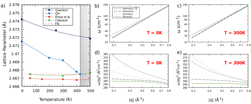
Figure 1: (a) Lattice parameter of graphene as a function of temperature obtained with the SCHA using a machine learning atomistic potential. Both quantum and classical calculations are included. The temperature-independent frozen nuclei (FN) result corresponds to the lattice parameter that minimizes the Born Oppenheimer potential $V$. The MD results obtained by Rowe et al. [44] are included. The lattice parameter calculated in the quasiharmonic (QH) approximation is also included. In the grey zone harmonic phonons become unstable breaking down the quasiharmonic approximation. (b)-(e) Harmonic ZA phonon spectra together with the SCHA auxiliary phonons and the physical phonons obtained from the peaks of the Green’s function in Eq. (2) at 0 K (b) and 300 K (c). Panels (d) and (e) show the bending rigidity, defined as the frequency divided by the squared momentum. In the panels the dispersion corresponds to the $\Gamma$M direction. For reference, the M point is at $1.4662$ $\AA^{-1}$ at $0$ K and at $1.4671$ $\AA^{-1}$ at $300$ K. The harmonic result (solid black) is computed at the lattice parameter that minimizes $V$, while the other results include thermal expansion. The dashed black lines correspond to harmonic calculations including thermal expansion (TE).

In order to preserve rotational symmetry, we make sure that the lattice parameter in our calculations sets the SCHA stress tensor [43] to zero at each temperature. The lattice parameter calculated in this way includes anharmonic effects as well as the effect of quantum and thermal fluctuations. All the phonon spectra shown in this work obtained with the atomistic potential are calculated with the lattice parameter that gives a null stress at each temperature. The harmonic spectra on the contrary are always calculated at the lattice parameter that minimizes $V$. The temperature dependence of the lattice parameter is shown in Fig. 1. We include the molecular dynamics (MD) results of Rowe et al. obtained with the same potential [44], which do not account for quantum effects. For comparison, we also include SCHA calculations in the classical limit, by making $\hbar=0$ in $\rho_{\bm{\mathcal{R}}\bm{\Phi}}$, and within the quasiharmonic (QH) approximation. Our quantum calculations correctly capture the negative thermal expansion of graphene that has been estimated in previous theoretical works [44, 28]. Our SCHA result shows a larger lattice parameter than the classical result. This is not surprising as classical calculations neglect quantum fluctuations and, consequently, underestimate the fluctuations associated to the high-energy optical modes (the highest energy phonon modes require temperatures of around 2000 K to be thermally populated). This remarks the importance of considering quantum effects in the evaluation of thermodynamic properties of graphene. Our classical results and the MD calculations of Rowe et al. [44] are in agreement at low temperatures.

In Figs. 1 (b)-(e) we compare the harmonic phonon spectra with the auxiliary phonons as well as with the spectra obtained from the peaks in the imaginary part of the interacting Green’s function, the physical phonons. The main conclusion is that while the dispersion of the ZA modes obtained from $\bm{\Phi}$ is linearized, the physical phonons become close to a quadratic dispersion and approach the harmonic dispersion, as expected by symmetry in the static limit. This is very clear in Fig. 1(d) and (e), where we show that the bending rigidity, defined as the frequency divided by the squared momentum, is independent of the wavevector at any temperature. This suggests that the bending rigidity is barely affected by interactions, in contradiction to the broadly assumed result that it diverges at small momentum in membranes due to thermal fluctuations [6].

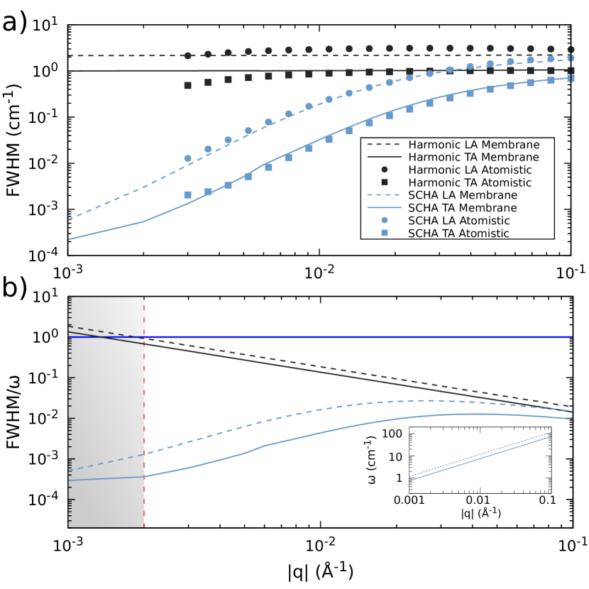
Figure 2: (a) Linewidths (full width at half maximum) of LA and TA phonon modes at $300$ K calculated within perturbation theory on top of the harmonic result and within the SCHA following Eq. (2). Squares and circles are calculated with the atomistic potential and lines correspond to calculations within the membrane model. Our harmonic results are in good agreement with other theoretical calculations [23, 24]. (b) FWHM divided by the phonon frequency in the membrane model. In the inset we show the phonon frequencies in the same momentum range. The grey zone corresponds to the region where the fraction FWHM${}_{LA}/\omega_{LA}$ is bigger than one in the harmonic case.

Even if the anharmonic correction to the phonon spectra may look small in Fig. 1, it has a huge impact on the acoustic properties of graphene. As shown in Fig. 2, the SCHA non-perturbative calculation based on Eq. (2) dramatically changes the linewidth of the LA and TA modes at small momenta by making them smaller as momentum decreases, in clear contrast to the perturbative calculation obtained on top of the harmonic result. This happens thanks to the linearization of the auxiliary flexural phonons that form the non-interacting Green’s function and enter in Dyson’s equation. When the ratio between the full-width at half-maximum (FWHM) and the frequency of the mode is approximately 1, the quasiparticle picture is lost. This value is reached in the 0.001-0.002 $\AA^{-1}$ momentum range in the harmonic case. However, when the linewidth is calculated within the SCHA, the ratio never gets bigger than 0.05. These results recover the quasiparticle picture for in-plane acoustic modes at any wavevector, guaranteeing that graphene always propagates sound. The momentum range for which the quasiparticle picture is lost in the harmonic approximation can be reached experimentally with Brillouin scattering probes. In fact, for few layer graphene the quasiparticle picture holds in the 0.001-0.002 $\AA^{-1}$ region [47], in agreement with our calculations. We show here that there is no need of strain [24] to have physically well-defined phonon linewidths in graphene.

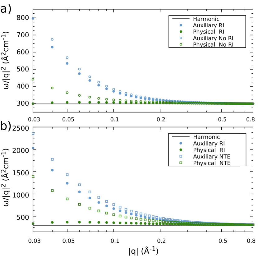
Figure 3: (a) Bending rigidity of graphene, defined as the ratio between the frequency of the ZA mode divided by the squared momentum, calculated within the harmonic approximation and within the SCHA auxiliary and physical cases at 0 K in the membrane model. We name rotationally invariant (RI) the results considering the full potential in Eq. 3. We name no rotationally invariant (No RI) the results neglecting the $\partial_{i}\bm{u}\cdot\partial_{j}\bm{u}$ term in Eq. (4). (b) Same results at $300$ K with the full membrane potential in the rotationally invariant case. We also include the results without considering thermal expansion (NTE).

In order to obtain results at very small momenta and reinforce the conclusions drawn with the atomistic calculations, we solve the SCHA equations in a continuum membrane Hamiltonian. This model has been widely used in the literature to describe graphene as an elastic membrane as well as to account for the coupling between in-plane and out-of plane acoustic modes [6, 34, 29, 30, 31]. The most general rotationally invariant continuum potential to describe a free-standing 2D membrane up to the fourth-order in the phonon fields has the following form [48]:

$$V = \frac{1}{2}\int_{\Omega}d^{2}x\left(\kappa(\partial^{2}h)^{2}+C^{ijkl}u_{ij}u_{kl}\right),$$ (3)

$$u_{ij} = \frac{1}{2}\left(\partial_{i}u_{j}+\partial_{j}u_{i}+\partial_{i}\bm{u}\cdot\partial_{j}\bm{u}+\partial_{i}h\partial_{j}h\right).$$ (4)

Here $\bm{u}(\bm{x})$ and $h(\bm{x})$ are the in-plane and out-of-plane displacement fields, respectively, $u_{ij}$ is the stress tensor, and $\bm{x}$ is the 2D position vector in the membrane. $\kappa$ is the harmonic bending rigidity of the membrane, $\Omega$ is the area of the membrane, and the tensor $C^{ijkl}=\lambda\delta^{ij}\delta^{kl}+\mu(\delta^{ik}\delta^{jl}+\delta^{il}\delta^{jk})$ contains the Lamé coefficients $\lambda$ and $\mu$ and Kronecker deltas. We have calculated the parameters by fitting them to the atomistic potential, which yields $\lambda=4.3$ eV$\AA^{-2}$, $\mu=9.3$ eV$\AA^{-2}$, $\kappa=1.5$ eV and, $\rho/\hbar^{2}=1097$ eV${}^{-1}\AA^{-4}$. This continuum model only accounts for acoustic modes. The harmonic acoustic frequencies given by Eq. (3) are $\omega_{ZA}(q)=\sqrt{\kappa/\rho}q^{2}$, $\omega_{LA}(q)=\sqrt{(\lambda+\mu)/\rho}q$, and $\omega_{TA}(q)=\sqrt{\mu/\rho}q$, $\rho$ being the mass density of the membrane. The thermal expansion is included in this formalism by changing the in-plane derivatives as $\partial_{i}u_{j}\rightarrow\partial_{i}u_{j}+\delta^{ij}\delta a$, with $\delta a=(a-a_{0})/a_{0}$, $a_{0}$ being the lattice parameter that minimizes $V$.

The results obtained in this rotationally invariant membrane are shown in Fig. 3. All conclusions drawn with the atomistic model are confirmed and put in solid grounds. Again the ZA phonons obtained from the auxiliary SCHA force constants get linearized at small momenta. However, when the physical phonons are calculated from the Hessian of the free energy (due to the low frequencies of the ZA modes this static approximation is perfectly valid as shown in the Methods section), the ZA phonon frequencies get on top of the harmonic values recovering a quadratic dispersion. This means that the physical phonons have a quadratic dispersion for small momenta in an unstrained membrane, as it is expected by symmetry, and that the bending rigidity does not increase in the long wavelength limit and is barely affected by interactions. Consequently the bending rigidity that we obtain is around the harmonic value of 1.5 eV, in good agreement with the consistent experiments by Al Taleb et al. [38] and Tømterud et al. [40]. Fig. 3 remarks that accounting correctly for the thermal expansion is crucial to recover the quadratic dispersion of the flexural modes. The validity of the membrane potential is confirmed by calculating the linewidths of the LA and TA modes, which yield consistent results to those obtained with the atomistic potential (see. Fig. 2).

Our results thus upturn the conventional wisdom of 2D membranes [6, 34, 29, 30, 31]: interactions do not linearize the dispersion of the ZA mode and the bending rigidity does not diverge at small momentum. The main reason for this is that in previous works the $\partial_{i}\bm{u}\cdot\partial_{j}\bm{u}$ term in the stress tensor, which guarantees rotational invariance, is neglected, unavoidably lowering the power of the ZA phonon frequency to $\sim q^{d}$ as shown in Fig. 3(a), with $d\sim 1.6$ in our case. The amplitude of the height fluctuations or ripples in the long wavelength limit reflects as well the absence of rotational symmetry in prior calculations. Different calculations within the self-consistent screening approximation or non-perturbative renormalization group theory yield consistent values of $\langle|h(\mathbf{q})|^{2}\rangle\sim q^{-4+\eta}$, with $\eta\sim 0.80-0.85$ [6, 34, 29, 30, 31, 49, 50]. We can estimate $\langle|h(\mathbf{q})|^{2}\rangle$ within the SCHA in our membrane model by calculating the equal time out-of-plane displacement correlation function, which in the static limit leads to the simple

$$\langle|h(\textbf{q})|^{2}\rangle=\frac{\left(1+2n_{B}(\Omega_{ZA}(\textbf{q}))\right)}{2\rho\Omega_{ZA}(\textbf{q})}$$ (5)

equation (see Methods), where $n_{B}(\omega)$ is the bosonic occupation factor and $\Omega_{ZA}(\textbf{q})$ the physical flexural phonon frequency coming from the free energy Hessian. The presence of the bosonic occupation completely determines the dependence on q of the correlation function: in the classical limit, when temperature is larger than the frequency of the ZA mode, $\langle|h(\textbf{q})|^{2}\rangle\sim\Omega_{ZA}(\textbf{q})^{-2}$, while in the quantum limit, when the ZA mode is unoccupied, $\langle|h(\textbf{q})|^{2}\rangle\sim\Omega_{ZA}(\textbf{q})^{-1}$. In the classical regime we recover the $\langle|h(\textbf{q})|^{2}\rangle\sim q^{-3.2}$ behavior when we neglect $\partial_{i}\bm{u}\cdot\partial_{j}\bm{u}$, consistently with previous results (see Fig. 4). However, when we keep full rotational invariance, the ZA modes acquires a quadratic dispersion and thus $\langle|h(\textbf{q})|^{2}\rangle\sim q^{-4}$, which is the result obtained in the harmonic case. Consequently, anharmonicity does not suppress the amplitude of the ripples in the long wavelength limit, upturning the previous consensus [6, 34, 29, 30, 31]. It is worth noting that the non rotational invariant membrane deviates from the $q^{-4}$ power law below a critical wave number [50].

The crossover between the regimes in which thermal and quantum fluctuations determine the ripples (see Fig. 4) is in very good agreement with the conclusions drawn with atomistic path-integral Monte Carlo simulations (PIMC) of freestanding graphene [51]. This crossover occurs at different wave numbers depending on the temperature, basically when $\hbar\Omega_{ZA}(\textbf{q})\sim k_{B}T$. However, atomistic classical Monte Carlo and MD simulations have estimated $\langle|h(\textbf{q})|^{2}\rangle$ for small wave numbers in the order of $q\sim 0.01\AA^{-1}$ finding a scaling law not far from the $q^{-3.2}$ obtained in the membrane model when rotational symmetry is broken [51, 7, 26, 50, 52]. Even if this contradicts our results since such atomistic calculations respect in principle rotational symmetry, an uncontrollable strain in the numerical simulations as small as $\delta a=10^{-5}$ is enough to lower the exponent from $-4$ to $-3.2$ in the long wave-length limit (see Methods). Considering that the ZA mode with $q\sim 0.01\AA^{-1}$ requires about 1 nanosecond to perform one period, very long simulation times are required to describe a thermodynamically flat phase of graphene, and, thus, these Monte Carlo and MD numerical simulations may also be affected by non-ergodic conditions, affecting the determination of the height correlation function in the long wavelength limit. On the contrary, in our SCHA simulations the centroids are always in the plane.

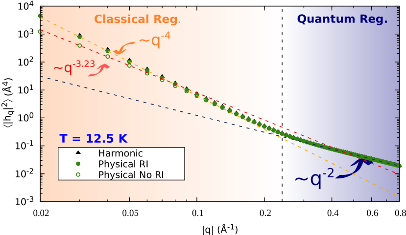
Figure 4: Fourier transform of the height-height correlation function at 12.5 K in the membrane model evaluated at different levels of approximation: harmonic (black dots), anharmonic RI result (green filled dots) and anharmonic No RI result (green empty dots). The dashed vertical line specifies the wavevector at which the crossover from classical (orange background) to quantum correlations (violet background) occurs at this temperature. The dashed lines correspond to linear fits with different exponents.

In conclusion, we show that anharmonic effects are crucial to make sound propagate in graphene despite its out-of-plane acoustic mode has a quadratic dispersion as imposed by symmetry. Contrary to the previously assumed behavior, we determine that the bending rigidity of graphene does not diverge in the long wavelength limit and that the amplitude of the ripples are not suppressed by phonon-phonon interactions. These conclusions are universal and can be extrapolated to any strictly 2D material or membrane.

Methods

Anharmonic theory: SCHA. We study the lattice dynamics of graphene in the Born-Oppenheimer (BO) approximation, thus we consider the quantum Hamiltonian for the atoms defined by the BO potential energy $V(\mathbf{R})$. With $\mathbf{R}$ we are denoting in component-free notation the quantity $R^{s\alpha}(\mathbf{l})$, which is a collective coordinate that completely specifies the atomic configuration of the crystal. The index $\alpha$ denotes the Cartesian direction, $s$ labels the atom within the unit cell and $\mathbf{l}$ indicates the three dimensional lattice vector. In what follows we will also use a single compact index $a=(\alpha,s,\mathbf{l})$ to indicate Cartesian index $\alpha$, atom $s$ index and lattice vector $\mathbf{l}$. Moreover, in general, we will use bold letters to indicate also other quantities in component-free notation.

In order to take into account quantum effects and anharmonicity at a non-perturbative level, we use the Self-Consistent Harmonic Approximation [42, 41, 43] (SCHA). For a given temperature $T$, the method allows to find an approximation for $F(\bm{\mathcal{R}})$, the free energy of the crystal as a function of the average atomic positions $\mathcal{R}^{a}$ (the centroids). For a given centroid $\bm{\mathcal{R}}$, the SCHA free energy is obtained through an auxiliary quadratic Hamiltonian, the SCHA Hamiltonian $\mathcal{H}_{\bm{\mathcal{R}}\bm{\Phi}}$, by variationally minimizing the free energy with respect to the SCHA centroids and auxiliary force-constants $\bm{\Phi}$. The free energy Hessian, or the physical phonons in the static approach, can be computed by using the analytic formula (in component-free notation)

$$\frac{\partial^{2}F}{\partial\bm{\mathcal{R}}\partial\bm{\mathcal{R}}}=\mathbf{\Phi}+\overset{(3)}{\mathbf{\Phi}}\mathbf{\Lambda}(0)[\mathbf{1}-\overset{(4)}{\mathbf{\Phi}}\mathbf{\Lambda}(0)]^{-1}\overset{(3)}{\mathbf{\Phi}},$$ (6)

with

$$\begin{split}\overset{(3)}{\mathbf{\Phi}}=\left\langle\frac{\partial^{3}V}{\partial\mathbf{R}\partial\mathbf{R}\partial{\mathbf{R}}}\right\rangle_{\rho_{\bm{\mathcal{R}}\bm{\Phi}}}&\;\overset{(4)}{\mathbf{\Phi}}=\left\langle\frac{\partial^{4}V}{\partial\mathbf{R}\partial\mathbf{R}\partial\mathbf{R}\partial\mathbf{R}}\right\rangle_{\rho_{\bm{\mathcal{R}}\bm{\Phi}}},\end{split}$$ (7)

where the averages are with respect to the density matrix of the SCHA Hamiltonian $\mathcal{H}_{\bm{\mathcal{R}}\bm{\Phi}}$, i.e. $\rho_{\bm{\mathcal{R}}\bm{\Phi}}=e^{-\beta\mathcal{H}_{\bm{\mathcal{R}}\bm{\Phi}}}/tr[e^{-\beta\mathcal{H}_{\bm{\mathcal{R}}\bm{\Phi}}}]$, and $\beta=(K_{B}T)^{-1}$ where $K_{B}$ is the Boltzmann constant. In Eq. (6) the value $z=0$ of the 4th-order tensor $\mathbf{\Lambda}(z)$ is used. For a generic complex number $z$ it is defined, in components, by

$$\mathbf{\Lambda}^{abcd}(z)=-\frac{1}{2}\sum_{\mu\nu}\tilde{F}(z,\omega_{\mu},\omega_{\nu})\times\\ \times\sqrt{\frac{\hbar}{2M_{a}\omega_{\mu}}}e_{\mu}^{a}\sqrt{\frac{\hbar}{2M_{b}\omega_{\nu}}}e_{\nu}^{b}\sqrt{\frac{\hbar}{2M_{c}\omega_{\mu}}}e_{\mu}^{c}\sqrt{\frac{\hbar}{2M_{d}\omega_{\nu}}}e_{\nu}^{d},$$ (8)

with $M_{a}$ the mass of the atom $a$, $\omega_{\mu}^{2}$ (the auxiliary phonons) the eigenvalues and $e_{\mu}^{a}$ the eigenvectors of $D_{ab}^{(S)}=\Phi_{ab}/\sqrt{M_{a}M_{b}}$, respectively, and

$$\tilde{F}(z,\omega_{\mu},\omega_{\nu})=\frac{2}{\hbar}\Bigg{[}\frac{(\omega_{\mu}+\omega_{\nu})[1+n_{B}(\tilde{\Omega}_{\mu})+n_{B}(\omega_{\nu})]}{(\omega_{\mu}+\omega_{\nu})^{2}-z^{2}}\\ -\frac{(\omega_{\mu}-\tilde{\Omega}_{\nu})[n_{B}(\omega_{\mu})-n_{B}(\omega_{\nu})]}{(\omega_{\mu}-\omega_{\nu})^{2}-z^{2}}\Bigg{]}$$ (9)

where $n_{B}(\omega)=1/(e^{\beta\hbar\omega}-1)$ is the bosonic occupation number.

As shown in Refs.  [41, 45, 46], in the SCHA the Green function $\mathbf{G}(i\Omega_{n})$for the correlation of variable $\sqrt{M_{a}}(R^{a}-\mathcal{R}^{a})$ in the frequency domain ($\Omega_{n}$ is a Matsubara frequency) is given as

$$\mathbf{G}^{-1}(i\Omega_{n})=(i\Omega_{n})^{2}\mathbf{1}-\mathbf{M}^{-\frac{1}{2}}\mathbf{\Phi}\mathbf{M}^{-\frac{1}{2}}-\mathbf{\Pi}(i\Omega_{n}),$$ (10)

where $\mathbf{G}^{-1}(0)=-\mathbf{D}^{(F)}$, $D_{ab}^{(F)}=\frac{1}{\sqrt{M_{a}M_{b}}}\frac{\partial^{2}F}{\partial\mathbf{\mathcal{R}}_{a}\partial\mathbf{\mathcal{R}}_{b}}$, and $\bm{\Pi}(z)$ is the SCHA self-energy, given by

$$\bm{\Pi}(i\Omega_{n})=\mathbf{M}^{-\frac{1}{2}}\overset{(3)}{\mathbf{\Phi}}\mathbf{\Lambda}(i\Omega_{n})[\mathbf{1}-\overset{(4)}{\mathbf{\Phi}}\mathbf{\Lambda}(i\Omega_{n})]^{-1}\overset{(3)}{\mathbf{\Phi}}\mathbf{M}^{-\frac{1}{2}},$$ (11)

where $M_{ab}=\delta_{ab}M_{a}$ is the mass matrix. For the applications considered in the present paper, the static term $\overset{(4)}{\mathbf{\Phi}}\mathbf{\Lambda}(0)$ is negligible with respect to the identity matrix (see Extended Data Fig. 1). Extending this approximation to the dynamical case reduces the SCHA self-energy to the so called bubble self-energy, namely

$$\mathbf{\Pi}\approx\mathbf{\Pi}^{(B)}(i\Omega_{n})=\mathbf{M}^{-\frac{1}{2}}\overset{(3)}{\mathbf{\Phi}}\mathbf{\Lambda}(i\Omega_{n})\overset{(3)}{\mathbf{\Phi}}\mathbf{M}^{-\frac{1}{2}}.$$ (12)

We then neglect the mixing between different phonon modes and assume that $\mathbf{\Pi}(i\Omega_{n})$ is diagonal in the basis of the eigenvectors $e_{\mu}^{a}(\mathbf{q})$ of $\Phi_{ab}(\mathbf{q})/\sqrt{M_{a}M_{b}}$ where $\Phi_{ab}(\mathbf{q})$ is the Fourier transform of the real space $\bm{\Phi}$ (now $a$ and $b$ represent atoms in the unit cell and Cartesian indices). We then define

$$\Pi_{\mu}(\mathbf{q},i\Omega_{n})=\sum_{a,b}e_{\mu}^{a}(-\mathbf{q})\Pi_{ab}(\mathbf{q},i\Omega_{n})e_{\mu}^{b}(\mathbf{q}).$$ (13)

In studying the response of a lattice to inelastic scattering experiments we need the one-phonon spectral function. By using Eq. (10) for $\mathbf{G}(i\Omega_{n})$ we can calculate the cross-section $\sigma(\omega)=-\omega TrIm\mathbf{G}(\omega+i0^{+})/\pi$, whose peaks signal the presence of collective vibrational excitations (physical phonons in the dynamic approach) having certain energies. Again, we take advantage of the lattice periodicity and we Fourier transform the interesting quantities with respect to the lattice indices. In particular, we consider the Fourier transform of the SCHA self-energy, $\Pi_{ab}(\mathbf{q},i\Omega_{n})$. Neglecting the mixing between different modes, the cross section is then given by

$$\small\sigma(\mathbf{q},\omega)=\frac{1}{\pi}\sum_{\mu}\frac{-\omega Im\Pi_{\mu}(\mathbf{q},\omega)}{(\omega^{2}-\omega_{\mu}^{2}(\mathbf{q})-Re\Pi_{\mu}(\mathbf{q},\omega))^{2}+(Im\Pi_{\mu}(\mathbf{q},\omega))^{2}}.$$ (14)

If we neglect the frequency dependence of the phonon self-energy, we get the weakly anharmonic limit of the cross section, which is going to be a sum of Lorentzian functions. These Lorentzians are well defined physical phonons in the dynamical approach. The phonon frequencies squared, $\Theta_{\mu}^{2}(\mathbf{q})$, corrected by the bubble self-energy are obtained as

$$\Theta_{\mu}^{2}(\mathbf{q})=\omega_{\mu}^{2}(\mathbf{q})+Re\Pi_{\mu}(\mathbf{q},\omega_{\mu}(\mathbf{q})),$$ (15)

where $\omega_{\mu}^{2}(\mathbf{q})$ are the eigenvalues of the Fourier transform of $\mathbf{D}^{(S)}$. The linewidth of the phonons in Eq. (15) is proportional to $Im\Pi_{\mu}(\mathbf{q},\omega_{\mu}(\mathbf{q}))$. The centers of these peaks are the ones supposed to be measured in inelastic experiments. By calculating $\Omega_{\mu}^{2}(\mathbf{q})=\omega_{\mu}^{2}(\mathbf{q})+Re\Pi_{\mu}(\mathbf{q},0)$ the static limit in Eq. (6) is recovered, i.e., the eigenvalues of the free energy Hessian. We show in Extended Data Fig. 2 that the dynamic effects are negligible in the ZA modes, meaning that the static approximation and the phonons coming from the free energy Hessian are a good approximation for the physical phonons.

Empirical potential benchmark and calculation parameters of the atomistic calculations. For calculating the forces needed in the atomistic SCHA minimization [42] we have used an empirical potential trained with machine learning and density functional theory (DFT) forces. The details about the machine learning training are explained in Ref.  [44]. Here we have benchmarked the ability of the potential to account for anharmonic effects. For that purpose we have applied the SCHA method by using DFT and empirical forces in a $2\times 2$ supercell and we have checked the anharmonic effects in the optical modes at the $\Gamma$ point. The machine learning potential is trained with the exchange-correlation in Ref.  [53] and for the DFT calculations we have applied a PBE [54] ultrasoft pseudopotential [55] with Van der Walls corrections [56]. The results are shown in Extended Data Figs. 3 and 4. As we can see in Extended Data Fig. 3, the two potentials provide very similar harmonic phonons. Due to the different exchange correlation functional there is a slight offset in Extended Data Fig. 4, however, the anharmonic lineshifts are very well captured within the empirical potential.
For the self-consistent DFT calculations used in the benchmark we have used a plane wave cutoff of $70$ Ry and a $700$ Ry cutoff for the density. For the Brillouin zone integration we have used a Monkhorst pack grid [57] of $32\times 32$ points with a Gaussian smearing of $0.02$ Ry.

The atomistic calculations of the linewidth in the main text have been performed with a grid of $400\times 400$ momentum points for the bubble self-energy, with a Gaussian smearing ($\delta$) of $1$ cm^-1. For the stress calculation in order to account for the thermal expansion we have used a $10\times 10$ supercell. We have used the same supercell for the SCHA auxiliary and physical frequency calculations in the atomistic case. For the linewidth calculations we have used $\overset{(3)}{\mathbf{\Phi}}$ calculated in a $3\times 3$ supercell and fourier interpolate it. We have tested all the calculations with denser grids and bigger supercells.

SCHA applied to the continuum membrane Hamiltonian. The general rotationally invariant potential for a membrane can be written as follows

$$V=\frac{1}{2}\int_{\Omega}{d^{2}x\left(\kappa(\partial^{2}h)^{2}+\sum_{n\geq 2}u_{i_{1}j_{1}}\dots u_{i_{n}j_{n}}C_{i_{1}j_{1}\dots i_{n}j_{n}}^{(2n)}\right)},$$ (16)

where $\Omega$ is the area of the membrane in equilibrium, $\kappa$ is the bending rigidity, $h$ is the out-of-plane component of the displacement field and the rotationally invariant strain tensor $u_{ij}$ is defined using the in-plane displacement field $u_{i}$

$$u_{ij}=\frac{1}{2}(\partial_{i}u_{j}+\partial_{j}u_{i}+\partial_{i}\bm{u}\cdot\partial_{j}\bm{u}+\partial_{i}h\partial_{j}h).$$ (17)

$C^{(2n)}_{i_{1}j_{1}\dots i_{n}j_{n}}$ is the generic elastic tensor of rank $2n$. In the previous expression the subscripts label the 2D coordinates $x,y$ and the sum over indices is assumed. The second-order expansion of Eq. (16) with respect to the phonon fields is given by

$$V=\frac{1}{2}\int_{\Omega}{d^{2}x\left(\kappa(\partial^{2}h)^{2}+C^{(4)}_{ijkl}u_{ij}u_{il}\right)},$$ (18)

with $C^{(4)}_{ijkl}=\lambda\delta_{ij}\delta_{kl}+\mu(\delta_{ik}\delta_{jl}+\delta_{il}\delta_{jk})$. By using equation (17) and $C_{ijkl}^{(4)}=C^{ijkl}$, equation (18) can be rewritten as

$$V=\frac{1}{2}\int_{\Omega}d^{2}x[\kappa(\partial^{2}h)^{2}+C^{ijkl}\partial_{i}u_{j}\partial_{k}u_{l}+C^{ijkl}\partial_{i}u_{j}\partial_{k}h\partial_{l}h+\\ +\frac{C^{ijkl}}{4}\partial_{i}h\partial_{j}h\partial_{k}h\partial_{l}h+\frac{C^{ijkl}}{2}\partial_{i}\bm{u}\cdot\partial_{j}\bm{u}\partial_{k}h\partial_{l}h+\\ +C^{ijkl}\partial_{i}u_{j}\partial_{k}\bm{u}\cdot\partial_{l}\bm{u}+\frac{C^{ijkl}}{4}\partial_{i}\bm{u}\cdot\partial_{j}\bm{u}\partial_{k}\bm{u}\cdot\partial_{l}\bm{u}].$$ (19)

If we allow the lattice spacing $a$ to be a variable, we can vary it by simply shifting the derivatives of the in-plane displacements according to $\partial_{i}u_{j}\rightarrow\partial_{i}u_{j}+\delta^{ij}\delta a$, where $\delta a=(a-a_{0})/a_{0}$. Then, by taking into account periodic boundary conditions, $\int_{\Omega}{d^{2}x\partial_{i}u_{j}}=0$, and we can rewrite the potential as

$$\small V\rightarrow V+2\Omega(1+\delta a)(\lambda+\mu)\delta a^{2}+\\ +(1+\frac{\delta a}{2})\delta a(\lambda+\mu)\int_{\Omega}{d^{2}x\partial_{k}h\partial_{k}h}+\\ +\frac{\delta a}{2}\int_{\Omega}{d^{2}xC^{ijkl}\partial_{i}u_{j}\partial_{k}h\partial_{l}h}+\\ +(1+\frac{\delta a}{2})\delta a\int_{\Omega}{d^{2}xC^{ijkl}\partial_{i}u_{j}\partial_{k}u_{l}}+\\ +(1+\frac{\delta a}{2})\delta a(\lambda+\mu)\int_{\Omega}{d^{2}x\partial_{k}\bm{u}\cdot\partial_{k}\bm{u}}+\frac{\delta a^{4}\Omega}{2}(\lambda+\mu)+\\ +\frac{\delta a}{4}\int_{\Omega}{d^{2}xC^{ijkl}[\partial_{i}\bm{u}\cdot\partial_{j}\bm{u}\partial_{k}u_{l}+\partial_{i}u_{j}\partial_{k}\bm{u}\cdot\partial_{l}\bm{u}]}.$$ (20)

The displacement fields $\textbf{u}(\textbf{x}),h(\textbf{x})$ can be expanded in the following plane wave basis set:

$$\textbf{u}(\textbf{x})=\frac{1}{\sqrt{\Omega}}\sum_{\textbf{q}}\textbf{u}(\textbf{q})e^{i\textbf{q}\cdot\textbf{x}},$$ (21)

$$h(\textbf{x})=\frac{1}{\sqrt{\Omega}}\sum_{\textbf{q}}h(\textbf{q})e^{i\textbf{q}\cdot\textbf{x}},$$ (22)

where q are discrete wavevectors determined by periodic boundary conditions and $\textbf{u}(\textbf{q}),h(\textbf{q})$ the corresponding Fourier transforms, which are defined according to

$$\textbf{u}(\textbf{q})=\frac{1}{\sqrt{\Omega}}\int_{\Omega}d^{2}x\;\textbf{u}(\textbf{x})e^{-i\textbf{q}\cdot\textbf{x}},$$ (23)

$$h(\textbf{q})=\frac{1}{\sqrt{\Omega}}\int_{\Omega}d^{2}x\;h(\textbf{x})e^{-i\textbf{q}\cdot\textbf{x}}.$$ (24)

Then, the SCHA free energy can be written as (we use $\hbar=k_{B}=1$):

$$\mathcal{F}(\mathcal{V})=F_{\mathcal{V}}+2\Omega(1+\delta a+\frac{\delta a^{2}}{4})(\lambda+\mu)\delta a^{2}+\\ +\frac{1}{2}\sum_{\bm{q}}\Biggl{\{}g[\omega_{SCHA}^{(h)}(\bm{q})]\kappa|\bm{q}|^{4}+\\ +\{(\lambda+2\mu)g[\omega_{SCHA}^{(LA)}(\bm{q})]+\mu g[\omega_{SCHA}^{(TA)}(\bm{q})]\}|\bm{q}|^{2}+\\ +\frac{\lambda+2\mu}{4\Omega}\sum_{\bm{k}}g[\omega_{SCHA}^{(h)}(\bm{q})]g[\omega_{SCHA}^{(h)}(\bm{k})][|\bm{q}|^{2}|\bm{k}|^{2}+2(\bm{q}\cdot\bm{k})^{2}]+\\ +\frac{1}{2\Omega}\sum_{\bm{k}}g[\omega_{SCHA}^{(h)}(\bm{k})]\{g[\omega_{SCHA}^{(LA)}(\bm{q})]+g[\omega_{SCHA}^{(TA)}(\bm{q})]\}\times\\ \times[\lambda|\bm{q}|^{2}|\bm{k}|^{2}+2\mu(\bm{q}\cdot\bm{k})^{2}]+\\ +2(1+\frac{\delta a}{2})\delta a(\lambda+\mu)g[\omega_{SCHA}^{(h)}(\bm{q})]|\bm{q}|^{2}+\\ +2(1+\frac{\delta a}{2})\delta a\{(\lambda+2\mu)g[\omega_{SCHA}^{(LA)}(\bm{q})]+\mu g[\omega_{SCHA}^{(TA)}(\bm{q})]\}|\bm{q}|^{2}+\\ +2(1+\frac{\delta a}{2})\delta a(\lambda+\mu)\{g[\omega_{SCHA}^{(LA)}(\bm{q})]+g[\omega_{SCHA}^{(TA)}(\bm{q})]\}|\bm{q}|^{2}+\\ +\frac{1}{4\Omega}\sum_{\bm{k}}\bigg{[}4g[\omega_{SCHA}^{(LA)}(\bm{q})]g[\omega_{SCHA}^{(TA)}(\bm{k})]\times\\ \times[\lambda(\bm{q}\cdot\bm{k})^{2}+\mu|\bm{q}|^{2}|\bm{k}|^{2}+\mu(\bm{q}\cdot\bm{k})^{2}](\hat{\bm{q}_{\perp}}\cdot\hat{\bm{k}})+\\ +2g[\omega_{SCHA}^{(LA)}(\bm{q})]g[\omega_{SCHA}^{(TA)}(\bm{k})][\lambda|\bm{q}|^{2}|\bm{k}|^{2}+2\mu(\bm{q}\cdot\bm{k})^{2}]+\\ +(g[\omega_{SCHA}^{(LA)}(\bm{q})]g[\omega_{SCHA}^{(LA)}(\bm{k})]+g[\omega_{SCHA}^{(TA)}(\bm{q})]g[\omega_{SCHA}^{(TA)}(\bm{k})])\times\\ \times[\lambda|\bm{q}|^{2}|\bm{k}|^{2}+2\mu(\bm{q}\cdot\bm{k})^{2}]+\\ 2(g[\omega_{SCHA}^{(LA)}(\bm{q})]g[\omega_{SCHA}^{(LA)}(\bm{k})])\times\\ \times[\lambda(\bm{q}\cdot\bm{k})^{2}+\mu|\bm{q}|^{2}|\bm{k}|^{2}+\mu(\bm{q}\cdot\bm{k})^{2}](\hat{\bm{q}}\cdot\hat{\bm{k}})+\\ +2(g[\omega_{SCHA}^{(TA)}(\bm{q})]g[\omega_{SCHA}^{(TA)}(\bm{k})])\times\\ \times[\lambda(\bm{q}\cdot\bm{k})^{2}+\mu|\bm{q}|^{2}|\bm{k}|^{2}+\mu(\bm{q}\cdot\bm{k})^{2}](\hat{\bm{q}_{\perp}}\cdot\hat{\bm{k}_{\perp}})\bigg{]}+\\ -\sum_{\alpha}g[\omega_{SCHA}^{(\alpha)}(\bm{q})]\Phi_{SCHA}^{(\alpha)}(\bm{q})\Biggr{\}},$$ (25)

where $g(\omega)=coth((\omega/2T))/(2\rho\omega)$ and $\omega_{SCHA}^{\alpha}(\bm{q})=\sqrt{\Phi_{SCHA}^{(\alpha)}(\bm{q})/\rho}$ ($\alpha=h,LA,TA$) is the SCHA auxiliary frequency. $\rho$ is the mass density. In Eq. (25) the in-plane displacement vector $\bm{u}(\bm{q}$) is separated into longitudinal and transversal components $\bm{u}(\bm{q})=u_{LA}(\bm{q})\hat{\bm{q}}+u_{TA}(\bm{q})\hat{\bm{q}_{\perp}}$, $\hat{\bm{q}}_{\perp}$ being the unitary vector perpendicular to $\hat{\bm{q}}$. $F_{\mathcal{V}}$ is the harmonic free energy of the harmonic auxiliary potential $\mathcal{V}$. Now, by taking the derivative of the SCHA free energy with respect to the lattice constant and SCHA auxiliary frequencies, we arrive to the SCHA equations:

$$\frac{\partial\mathcal{F}(\mathcal{V})}{\partial\delta a}=0=2\Omega(2\delta a+3\delta a^{2}+\delta a^{3})(\lambda+\mu)+\\ +\frac{1}{2}\sum_{\bm{q}}g[\omega_{SCHA}^{(h)}(\bm{q})]2(1+\delta a)(\lambda+\mu)|\bm{q}|^{2}+\\ +\frac{1}{2}\sum_{\bm{q}}g[\omega_{SCHA}^{(LA)}(\bm{q})][2(1+\delta a)(\lambda+2\mu)|\bm{q}|^{2}+2(1+\delta a)(\lambda+\mu)|\bm{q}|^{2}]+\\ +\frac{1}{2}\sum_{\bm{q}}g[\Omega_{SCHA}^{(TA)}(\bm{q})][2(1+\delta a)\mu|\bm{q}|^{2}+2(1+\delta a/2)(\lambda+\mu)|\bm{q}|^{2}],$$ (26)

$$\Phi_{SCHA}^{(h)}(\bm{q})=\kappa|\bm{q}|^{4}+2(1+\delta a/2)\delta a(\lambda+\mu)|\bm{q}|^{2}+\\ +\frac{\lambda+2\mu}{2\Omega}\sum_{\bm{k}}g[\omega_{SCHA}^{(h)}(\bm{k})][|\bm{q}|^{2}|\bm{k}|^{2}+2(\bm{q}\cdot\bm{k})^{2}]+\\ +\frac{1}{2\Omega}\sum_{\bm{k}}\{g[\omega_{SCHA}^{(LA)}(\bm{k})]+g[\omega_{SCHA}^{(TA)}(\bm{k})]\}[\lambda|\bm{q}|^{2}|\bm{k}|^{2}+2\mu(\bm{q}\cdot\bm{k})^{2}],$$ (27)

$$\Phi_{SCHA}^{(LA)}(\bm{q})=(\lambda+2\mu)|\bm{q}|^{2}+2(1+\delta a/2)\delta a(\lambda+2\mu)|\bm{q}|^{2}+\\ +2(1+\delta a/2)\delta a(\lambda+\mu)|\bm{q}|^{2}+\\ +\frac{1}{2\Omega}\sum_{\bm{k}}g[\omega_{SCHA}^{(h)}(\bm{k})][\lambda|\bm{q}|^{2}|\bm{k}|^{2}+2\mu(\bm{q}\cdot\bm{k})^{2}]+\\ +\frac{1}{4\Omega}\sum_{\bm{k}}\biggl{\{}4g[\omega_{SCHA}^{(TA)}(\bm{k})][\lambda(\bm{q}\cdot\bm{k})^{2}+\mu|\bm{q}|^{2}|\bm{k}|^{2}+\mu(\bm{q}\cdot\bm{k})^{2}](\hat{\bm{q}_{\perp}}\cdot\hat{\bm{k}})+\\ +2g[\omega_{SCHA}^{(TA)}(\bm{k})][\lambda|\bm{q}|^{2}|\bm{k}|^{2}+2\mu(\bm{q}\cdot\bm{k})^{2}]+\\ +2g[\omega_{SCHA}^{(LA)}(\bm{k})][\lambda|\bm{q}|^{2}|\bm{k}|^{2}+2\mu(\bm{q}\cdot\bm{k})^{2}]+\\ +4g[\omega_{SCHA}^{(LA)}(\bm{k})][\lambda(\bm{q}\cdot\bm{k})^{2}+\mu|\bm{q}|^{2}|\bm{k}|^{2}+\mu(\bm{q}\cdot\bm{k})^{2}](\hat{\bm{q}}\cdot\hat{\bm{k}})\biggr{\}}$$ (28)

and,

$$\Phi_{SCHA}^{(TA)}(\bm{q})=\mu|\bm{q}|^{2}+2(1+\delta a/2)\delta a\mu|\bm{q}|^{2}+\\ +2(1+\delta a/2)\delta a(\lambda+\mu)|\bm{q}|^{2}+\\ +\frac{1}{2\Omega}\sum_{\bm{k}}g[\omega_{SCHA}^{(h)}(\bm{k})][\lambda|\bm{q}|^{2}|\bm{k}|^{2}+2\mu(\bm{q}\cdot\bm{k})^{2}]+\\ +\frac{1}{4\Omega}\sum_{\bm{k}}\biggl{\{}4g[\omega_{SCHA}^{(TA)}(\bm{k})][\lambda(\bm{q}\cdot\bm{k})^{2}+\mu|\bm{q}|^{2}|\bm{k}|^{2}+\mu(\bm{q}\cdot\bm{k})^{2}](\hat{\bm{q}_{\perp}}\cdot\hat{\bm{k}_{\perp}})+\\ +4g[\omega_{SCHA}^{(LA)}(\bm{k})][\lambda(\bm{q}\cdot\bm{k})^{2}+\mu|\bm{q}|^{2}|\bm{k}|^{2}+\mu(\bm{q}\cdot\bm{k})^{2}](\hat{\bm{q}_{\perp}}\cdot\hat{\bm{k}})+\\ +2g[\omega_{SCHA}^{(TA)}(\bm{k})][\lambda|\bm{q}|^{2}|\bm{k}|^{2}+2\mu(\bm{q}\cdot\bm{k})^{2}]\biggr{\}}.$$ (29)

When solving this set of equations, it has been taken into account that the assumed periodic boundary conditions make the reciprocal space discrete. In order to reach wave vectors a magnitude of order smaller than in our atomistic calculations, we have worked with a squared membrane of size $L_{x}=L_{y}=\frac{2\pi}{0.01}\AA$. On the other side, the implicit continuity of the membrane Hamiltonian makes Fourier transforms to be non-periodic. Then, as displacement fields u(x) and h(x) are smooth functions in real space, their discrete and non-periodic Fourier transforms u(q) and h(q) (and related magnitudes) are expected to decay rapidly in reciprocal space. Therefore, we can converge our results with respect to a cut-off radius in momentum space, defining in this way a circular grid. The value of this cut-off radius is temperature dependent, because modes with greater q values are thermally excited when increasing the temperature. We have found that with a value of R${}_{cut}=0.8$ $\AA^{-1}$ convergence is achieved for temperatures close to 0K. This radius encloses 20080 q-points, which yields a total of 60241 coupled equations that we have solved by applying the Newton-Raphson method [58]. This model accounts for the negative thermal expansion of graphene as it can be seen in Extended Data Fig. 5.

Regarding the second derivative of the free energy, the physical phonons in the static approach, the most general formula for the correction to the SCHA auxiliary phonon frequencies is

$$D_{\alpha\beta}^{corr}(-\bm{q},\bm{q})=\sum_{\gamma\delta\epsilon\zeta}\sum_{\bm{p}\bm{k}}\overset{(3)}{D}{}_{\alpha\gamma\delta}(-\bm{q},\bm{p},\bm{q}-\bm{p})\times\\ \times[1-\overset{(4)}{D}{}_{\gamma\delta\epsilon\zeta}(-\bm{p},\bm{p}-\bm{q},\bm{k},\bm{q}-\bm{k})]^{-1}\overset{(3)}{D}{}_{\epsilon\zeta\beta}(-\bm{k},\bm{k}-\bm{q},\bm{q}),$$ (30)

where the subindexes run on the normal coordinates $\alpha,\beta,\gamma,\delta,\epsilon,\zeta=h,u_{LA},u_{TA}$ and the dynamical matrices in normal coordinates are defined as

$$\overset{(3)}{D}{}_{\alpha\beta\gamma}(\bm{q},\bm{k},\bm{p})=\frac{1}{\rho^{3/2}}\left\langle\frac{\partial^{3}V}{\partial\alpha(\bm{q})\partial\beta(\bm{k})\partial\gamma(\bm{p})}\right\rangle_{\rho_{\mathcal{V}}}\sqrt{G_{\beta\gamma}(\bm{k},\bm{p})},$$ (31)

$$\overset{(4)}{D}{}_{\alpha\beta\gamma\epsilon}(\bm{q},\bm{q}^{\prime},\bm{k},\bm{k}^{\prime})=\frac{1}{\rho^{2}}\left\langle\frac{\partial^{4}V}{\partial\alpha(\bm{q})\partial\beta(\bm{q}^{\prime})\partial\gamma(\bm{k})\partial\epsilon(\bm{k}^{\prime})}\right\rangle_{\rho_{\mathcal{V}}}\\ \times\sqrt{G_{\alpha\beta}(\bm{q},\bm{k})G_{\gamma\epsilon}(\bm{q}^{\prime},\bm{k}^{\prime})}.$$ (32)

The matrix $G_{\alpha\beta}(\bm{q},\bm{k})$ is defined as

$$G_{\alpha\beta}(\bm{q},\bm{k})=\frac{F(0,\omega_{SCHA}^{\alpha}(\bm{q}),\omega_{SCHA}^{\beta}(\bm{k}))}{\omega_{SCHA}^{\alpha}(\bm{q})\omega_{SCHA}^{\beta}(\bm{k})},$$ (33)

$F(0,\omega_{SCHA}^{\alpha}(\bm{q}),\omega_{SCHA}^{\beta}(\bm{k}))$ being the function defined in Eq. (9). We are interested in the corrections to the out-of-plane modes, therefore, we are interested in the terms of the type

$$D_{hh}^{corr}(-\bm{q},\bm{q})=\sum_{\gamma\delta\epsilon\zeta}\sum_{\bm{p}\bm{k}}\overset{(3)}{D}{}_{h\gamma\delta}(-\bm{q},\bm{p},\bm{q}-\bm{p})\times\\ \times[1-\overset{(4)}{D}{}_{\gamma\delta\epsilon\zeta}(-\bm{p},\bm{p}-\bm{q},\bm{k},\bm{q}-\bm{k})]^{-1}\overset{(3)}{D}{}_{\epsilon\zeta h}(-\bm{k},\bm{k}-\bm{q},\bm{q}).$$ (34)

By looking at Eq. (20) we can see that only the terms of the type $\int_{\Omega}{d^{2}xC^{ijkl}\partial_{i}u_{j}\partial_{k}h\partial_{l}h}$ will contribute to the statistical average in Eq. (31). Therefore, Eq. (30) can be rewritten as

$$D_{hh}^{corr}(-\bm{q},\bm{q})=4\sum_{\alpha\beta}\sum_{\bm{p}\bm{k}}\overset{(3)}{D}{}_{hh\alpha}(-\bm{q},\bm{p},\bm{q}-\bm{p})\times\\ \times[1-\overset{(4)}{D}{}_{h\alpha h\beta}(-\bm{p},\bm{p}-\bm{q},\bm{k},\bm{q}-\bm{k})]^{-1}\overset{(3)}{D}{}_{h\beta h}(-\bm{k},\bm{k}-\bm{q},\bm{q}),$$ (35)

where now the subindexes only run in $\alpha,\beta=u_{LA},u_{TA}$. Now, we can calculate the statistical averages

$$\left\langle\frac{\partial^{3}V}{\partial h(\bm{k}_{1})\partial h(\bm{k}_{2})\partial u_{LA}(\bm{k}_{3})}\right\rangle_{\rho_{\mathcal{V}}}=\frac{1+\delta a}{\sqrt{\Omega}}\delta_{\bm{k}_{1}+\bm{k}_{2}+\bm{k}_{3},0}\times\\ \times\left[\lambda|\bm{k}_{3}|\bm{k}_{1}\cdot\bm{k}_{2}+2\mu\frac{(\bm{k}_{3}\cdot\bm{k}_{1})(\bm{k}_{3}\cdot\bm{k}_{2})}{|\bm{k}_{3}|}\right],$$ (36)

$$\left\langle\frac{\partial^{3}V}{\partial h(\bm{k}_{1})\partial h(\bm{k}_{2})\partial u_{TA}(\bm{k}_{3})}\right\rangle_{\rho_{\mathcal{V}}}=\frac{\mu(1+\delta a)}{\sqrt{\Omega}}\delta_{\bm{k}_{1}+\bm{k}_{2}+\bm{k}_{3},0}\times\\ \times\left[\frac{(\bm{k}_{3}\cdot\bm{k}_{1})(\bm{k}_{3\perp}\cdot\bm{k}_{2})+(\bm{k}_{3}\cdot\bm{k}_{2})(\bm{k}_{3\perp}\cdot\bm{k}_{1})}{|\bm{k}_{3}|}\right],$$ (37)

$$\left\langle\frac{\partial^{4}V}{\partial h(\bm{k}_{1})\partial h(\bm{k}_{2})\partial u_{LA}(\bm{k}_{3})\partial u_{LA}(\bm{k}_{4})}\right\rangle_{\rho_{\mathcal{V}}}=\\ \frac{1}{\Omega}\delta_{\bm{k}_{1}+\bm{k}_{2}+\bm{k}_{3}+\bm{k}_{4},0}\frac{\bm{k}_{3}\cdot\bm{k}_{4}}{|\bm{k}_{3}||\bm{k}_{4}|}[\lambda(\bm{k}_{3}\cdot\bm{k}_{4})(\bm{k}_{1}\cdot\bm{k}_{2})+\\ +\mu(\bm{k}_{3}\cdot\bm{k}_{1})(\bm{k}_{4}\cdot\bm{k}_{2})+\mu(\bm{k}_{3}\cdot\bm{k}_{2})(\bm{k}_{4}\cdot\bm{k}_{1})],$$ (38)

$$\left\langle\frac{\partial^{4}V}{\partial h(\bm{k}_{1})\partial h(\bm{k}_{2})\partial u_{TA}(\bm{k}_{3})\partial u_{TA}(\bm{k}_{4})}\right\rangle_{\rho_{\mathcal{V}}}=\\ \frac{1}{\Omega}\delta_{\bm{k}_{1}+\bm{k}_{2}+\bm{k}_{3}+\bm{k}_{4},0}\frac{\bm{k}_{3\perp}\cdot\bm{k}_{4\perp}}{|\bm{k}_{3}||\bm{k}_{4}|}[\lambda(\bm{k}_{3}\cdot\bm{k}_{4})(\bm{k}_{1}\cdot\bm{k}_{2})+\\ +\mu(\bm{k}_{3}\cdot\bm{k}_{1})(\bm{k}_{4}\cdot\bm{k}_{2})+\mu(\bm{k}_{3}\cdot\bm{k}_{2})(\bm{k}_{4}\cdot\bm{k}_{1})],$$ (39)

and

$$\left\langle\frac{\partial^{4}V}{\partial h(\bm{k}_{1})\partial h(\bm{k}_{2})\partial u_{LA}(\bm{k}_{3})\partial u_{TA}(\bm{k}_{4})}\right\rangle_{\rho_{\mathcal{V}}}=\\ \frac{1}{\Omega}\delta_{\bm{k}_{1}+\bm{k}_{2}+\bm{k}_{3}+\bm{k}_{4},0}\frac{\bm{k}_{3}\cdot\bm{k}_{4\perp}}{|\bm{k}_{3}||\bm{k}_{4}|}[\lambda(\bm{k}_{3}\cdot\bm{k}_{4})(\bm{k}_{1}\cdot\bm{k}_{2})+\\ +\mu(\bm{k}_{3}\cdot\bm{k}_{1})(\bm{k}_{4}\cdot\bm{k}_{2})+\mu(\bm{k}_{3}\cdot\bm{k}_{2})(\bm{k}_{4}\cdot\bm{k}_{1})].$$ (40)

The equations cannot be further simplified but we have all the ingredients to calculate them numerically. We have checked numerically that, as in the atomistic case, the contribution of $\overset{(4)}{\bm{D}}$ is completely negligible. To show that we Taylor expand Eq. (11)

$$\bm{\Pi}(z)=\mathbf{M}^{-\frac{1}{2}}\overset{(3)}{\mathbf{\Phi}}\mathbf{\Lambda}(z)[\mathbf{1}-\overset{(4)}{\mathbf{\Phi}}\mathbf{\Lambda}(z)]^{-1}\overset{(3)}{\mathbf{\Phi}}\mathbf{M}^{-\frac{1}{2}}\simeq\\ \simeq\mathbf{M}^{-\frac{1}{2}}\overset{(3)}{\mathbf{\Phi}}\mathbf{\Lambda}(z)\overset{(3)}{\mathbf{\Phi}}\mathbf{M}^{-\frac{1}{2}}+\mathbf{M}^{-\frac{1}{2}}\overset{(3)}{\mathbf{\Phi}}\mathbf{\Lambda}(z)\overset{(4)}{\mathbf{\Phi}}\mathbf{\Lambda}(z)\overset{(3)}{\mathbf{\Phi}}\mathbf{M}^{-\frac{1}{2}},$$ (41)

and we calculate the contribution of the term containing the fourth-order tensor to the linewidth. We also calculate the spectral function with and without including the frequency dependence of the self energy. We show the results in Extended Data Fig. 6. The figure clearly shows that the contribution of the fourth-order tensor is at least one order of magnitude smaller than the main term, justifying the bubble approximation of the self-energy, and, what it is more important, it also decays as momentum decreases. The figure also shows that the Lorentzian approximation is justified for the acoustic modes in graphene.

By neglecting the fourth-order terms containing in-plane displacement fields in Eq. 16, the SCHA can be applied analytically in this model. The SCHA equations simplify to

$$\delta a=-\frac{1}{4\Omega}\sum_{\bm{q}}|\bm{q}|^{2}g[\omega_{SCHA}^{(h)}(\bm{q})],$$ (42)

$$\Phi_{SCHA}^{(h)}(\bm{q})=\kappa|\bm{q}|^{4}+2\delta a(\lambda+\mu)|\bm{q}|^{2}+\\ +\frac{\lambda+2\mu}{2\Omega}\sum_{\bm{k}}g[\omega_{SCHA}^{(LA)}(\bm{k})][|\bm{q}|^{2}|\bm{k}|^{2}+2(\bm{q}\cdot\bm{k})^{2}].$$ (43)

By inserting Eq. (42) in Eq. (43) and considering the infinite volume limit ($\Omega\rightarrow\infty$), we obtain

$$\Phi_{SCHA}^{(h)}(\bm{q})=\kappa|\bm{q}|^{4}+\gamma|\bm{q}|^{2},$$ (44)

where $\gamma$ is given by the solution of

$$\gamma=\gamma\frac{\lambda+3\mu}{16\pi\kappa\sqrt{\rho\kappa}}\int_{0}^{\Lambda\sqrt{\kappa/\gamma}}ds\frac{s^{2}coth[\gamma s\sqrt{1+s^{2}}/(2T\sqrt{\rho\kappa})]}{\sqrt{1+s^{2}}}.$$ (45)

$\Lambda$ is an ultraviolet cutoff that avoids divergencies. Eqs. 44 and 45 show that the dispersion of the SCHA auxiliary ZA modes is linear. By calculating the correction for getting the physical phonons in the static approach in Eq. 35 (in this case the fourth-order tensor is $0$) the result is

$$\Phi_{F}^{(h)}(\bm{q})=\kappa|\bm{q}|^{4}+(\gamma-\sigma)|\bm{q}|^{2}+O(|\bm{q}|^{4}),$$ (46)

where at $T=0$ K

$$\sigma=\frac{\rho\sqrt{\gamma}}{8\pi\kappa^{3/2}}\sum_{\alpha=LA,TA}v_{\alpha}f(\Lambda\sqrt{\kappa/\gamma},v_{\alpha}\sqrt{\rho/\gamma}),$$ (47)

with

$$f(x,y)=\int_{0}^{x}ds\frac{s^{2}}{\sqrt{1+s^{2}}[\sqrt{1+s^{2}}+y]}.$$ (48)

By setting the ultraviolet cutoff to the value of the Debye momentum, $\Lambda=\sqrt{\frac{8\pi}{3^{1/2}a_{0}}}=1.55\AA$, we obtain $1-\sigma/\gamma=20\%$. This means that the linear component of the physical frequencies turns out to be a factor of $40\%$ smaller than the one of the SCHA auxiliary frequency. The non zero linear term in the physical frequencies appears because neglecting the fourth-order terms including in-plane displacements breaks the rotational invariance of the potential.

The equal time height-height correlation function within SCHA. Within an interacting picture, the ensemble average of any displacement-displacement correlation function is given by the following equal time Green function (we use $\hbar=k_{B}=1$):

$$\sqrt{M_{a}M_{b}}\langle u_{a}u_{b}\rangle=G^{ab}(\tau=0^{+})=-T\sum_{n}G^{ab}(i\Omega_{n}),$$ (49)

where $G^{ab}(i\Omega_{n})$ is the SCHA Green function in frequency domain for the variable $\sqrt{M_{a}}$($R^{a}-\mathcal{R}^{a}_{eq}$) defined in Eq. (2) and $\Omega_{n}=2\pi Tn$ are the bosonic Matsubara’s frequencies. $\mathcal{R}^{a}_{eq}$ are the centroid positions that minimize the SCHA free energy.

The summation has to be done via the Lehmann representation:

$$\sqrt{M_{a}M_{b}}\langle u_{a}u_{b}\rangle=-T\sum_{n}G^{ab}(i\Omega_{n})=\int_{-\infty}^{\infty}\frac{d\omega}{2\pi}\;\sigma(\omega)n_{B}(\omega)$$ (50)

being $\sigma(\omega)$ the spectral function of the Green function: $\sigma(\omega)=-2\text{Im}[G(\omega+i0^{+})]$. Retaining only the first term of the dynamical SCHA self energy (bubble aproximation) and neglecting the mode-mixing, the spectral function resembles a superposition of Lorentzians, but with frequency dependent shifts and widths. When the quasiparticle picture is valid after the inclusion of anharmonicity, the spectral function can actually be expressed as a superposition of Lorentzians:

$$\sigma(\omega)=\sum_{\mu}\epsilon_{\mu}^{a}\epsilon_{\mu}^{b}\Bigg{(}\frac{1}{\omega}\Bigg{[}\frac{\Gamma_{\mu}}{(\omega-\Theta_{\mu})^{2}+(\Gamma_{\mu})^{2}}+\\ +\frac{\Gamma_{\mu}}{(\omega+\Theta_{\mu})^{2}+(\Gamma_{\mu})^{2}}\Bigg{]}\Bigg{)},$$ (51)

where $\Theta_{\mu}$ is the frequency of the SCHA quasiparticle in the Lorentzian approximation and $\Gamma_{\mu}$ its HWHM linewidth.

We can avoid divergences in the integral by redefining the sum as

$$\sqrt{M_{a}M_{b}}\langle u_{a}u_{b}\rangle=-TG^{ab}(0)+\int_{-\infty}^{\infty}\frac{d\omega}{2\pi}\;\sigma(\omega)\left[n_{B}(\omega)-\frac{T}{\omega}\right].$$ (52)

Regarding the first term in the sum, the static limit of the Green function corresponds to the inverse of the free energy dynamical matrix:

$$G^{ab}(i\Omega_{n}=0)=-[D^{(F)}]^{-1}_{ab}=\sum_{\mu}\epsilon_{\mu}^{a}\epsilon_{\mu}^{b}\left(-\frac{1}{\Omega_{\mu}^{2}}\right),$$ (53)

where $\Omega_{\mu}$ are again the frequencies of the free energy phonons.

Inserting Eqs. (53) and (51) in Eq. (52):

$$\sqrt{M_{a}M_{b}}\langle u_{a}u_{b}\rangle=\sum_{\mu}\epsilon_{\mu}^{a}\epsilon_{\mu}^{b}\Bigg{(}\frac{T}{\Omega_{\mu}^{2}}+\int_{-\infty}^{\infty}\frac{d\omega}{2\pi}\times\\ \times\Big{(}\frac{1}{\omega}\left[\frac{\Gamma_{\mu}}{(\omega-\Theta_{\mu})^{2}+(\Gamma_{\mu})^{2}}+\frac{\Gamma_{\mu}}{(\omega+\Theta_{\mu})^{2}+(\Gamma_{\mu})^{2}}\right]\Big{)}\times\\ \times\left[n_{B}(\omega)-\frac{T}{\omega}\right]\Bigg{)}.$$ (54)

This integral can be simplified when the phonon-phonon linewidth tends to zero. For those cases, the Lorentzian representation of the Dirac delta function can be used:

$$\delta(x)=\frac{1}{\pi}\lim_{\epsilon\to 0^{+}}\frac{\epsilon}{x^{2}+\epsilon^{2}}.$$ (55)

Then,

$$\sqrt{M_{a}M_{b}}\langle u_{a}u_{b}\rangle=\sum_{\mu}\epsilon_{\mu}^{a}\epsilon_{\mu}^{b}\Bigg{(}\frac{T}{\Omega_{\mu}^{2}}+\frac{1}{2}\int_{-\infty}^{\infty}d\omega\times\\ \times\left(\frac{1}{\omega}\times\left[\delta(\omega-\Theta_{\mu})+\delta(\omega+\Theta_{\mu})\right]\right)\left[n_{B}(\omega)-\frac{T}{\omega}\right]\Bigg{)}.$$ (56)

And

$$\langle u_{a}u_{b}\rangle=\frac{\sum_{\mu}\epsilon_{\mu}^{a}\epsilon_{\mu}^{b}}{\sqrt{M_{a}M_{b}}}\left(\frac{T}{\Omega_{\mu}^{2}}+\frac{-\hbar n_{B}(-\Theta_{\mu})+\hbar n_{B}(\Theta_{\mu})}{2\Theta_{\mu}}-\frac{T}{\Theta_{\mu}^{2}}\right).$$

Finally, when free energy Hessian phonons (physical phonons in the static approach) and physical ones are nearly identical ($\Omega_{\mu}^{2}\approx\Theta_{\mu}^{2}$), we recover the formula of the non-interacting case but evaluated with free energy Hessian (equivalently, physical) phonons:

$$\begin{split}\langle u_{a}u_{b}\rangle&=\frac{\sum_{\mu}\epsilon_{\mu}^{a}\epsilon_{\mu}^{b}}{\sqrt{M_{a}M_{b}}}\left[\frac{\left(n_{B}[\Omega_{\mu}]-n_{B}[-\Omega_{\mu}]\right)}{2\Omega_{\mu}}\right]=\\ &=\frac{\sum_{\mu}\epsilon_{\mu}^{a}\epsilon_{\mu}^{b}}{\sqrt{M_{a}M_{b}}}\left[\frac{\left(1+2n_{B}[\Omega_{\mu}]\right)}{2\Omega_{\mu}}\right].\end{split}$$ (57)

In the case of the membrane model, the displacement-displacement correlation function is:

$$\langle u_{a}(\textbf{x})u_{b}(\textbf{x}^{\prime})\rangle=\frac{\sum_{\mu}\epsilon_{\mu}^{a}(\textbf{x})\epsilon_{\mu}^{b}(\textbf{x}^{\prime})}{\rho}\left[\frac{\left(1+2n_{B}[\Omega_{\mu}]\right)}{2\Omega_{\mu}}\right],$$ (58)

where $a$ and $b$ are the Cartesian indexes and $\mu=h,LA,TA$ in this case. Essentially, discrete magnitudes are now continuous, while the individual atomic masses $M_{a}$ and $M_{b}$ are replaced by the mass density of the membrane $\rho$. The corresponding Fourier transform is given by

$$\langle u_{a}(\textbf{q})u_{b}(\textbf{k})\rangle=\delta_{\textbf{q},-\textbf{k}}\frac{\sum_{\mu}\epsilon_{\mu}^{a}(\textbf{q})\epsilon_{\mu}^{b}(-\textbf{q})}{\rho}\left[\frac{\left(1+2n_{B}[\Omega_{\mu}(\textbf{q})]\right)}{2\Omega_{\mu}(\textbf{q})}\right].$$ (59)

We are particularly interested on the Fourier transform of the out-of-plane correlation function. As in the membrane model $ZA$ is the only mode with an out-of-plane component, we finally obtain:

$$\langle|h(\textbf{q})|^{2}\rangle=\frac{\left(1+2n_{B}[\Omega_{ZA}(\textbf{q})]\right)}{2\rho\Omega_{ZA}(\textbf{q})},$$ (60)

which is the formula implemented along this article to obtain the Fourier transform of the height-height correlation function.

Nearly all the approximations taken in this mathematical derivation have been proved for the graphene throughout this article. The only task left is showing that the linewidth of the ZA mode is as small as the ones corresponding to the in-plane phonon modes, which is indeed true as shown in Extended Data Fig. 7.

Extra calculations of the equal time height-height correlation function. The out-of-plane correlation function is governed by the bosonic occupation factor. Quantum correlations appear for those flexural modes that are barely occupied thermally, that is, in those modes which quantum zero-point energy is bigger than the thermal energy:

$$\frac{1}{2}\hbar\omega_{ZA}(\textbf{q})>K_{B}T<=>q_{T}>\left(\sqrt{\frac{\rho}{\kappa}}\frac{2K_{B}T}{\hbar}\right).$$ (61)

Decreasing the temperature and/or increasing the wavelength favours the emergence of quantum correlations  [51].

In this subsection we provide extra calculations analyzing the extreme cases at 0 K and 300 K. At null temperature there is no phonon mode thermally occupied, but all of them fluctuate due to quantum zero-point motion. The height-height correlation function shows then a fully quantum behaviour, with no crossover to a classical regime as shown in Extended Data Fig. 8. The harmonic and anharmonic rotational invariant results yield the same exponents due to their quadratic dispersion: $\langle|h(\textbf{q})|^{2}\rangle\sim q^{-2}$. The anharmonic non rotational invariant phonons are quadratic in the short wavelength limit, but they are linearized in the long wavelength limit with $\langle|h(\textbf{q})|^{2}\rangle\sim\Omega_{ZA}(\textbf{q})^{-1}\sim q^{-1.62}$. This exponent coincides with the one obtained in the self consistent screening approximation (SCSA), which scale as $q^{\nu}$ with $\nu\sim 1.6$ [50].

At 300 K the classic to quantum crossover occurs at 1.18 $\AA^{-1}$, so that all the modes are largely occupied in the $q$ range in which we have focused our analysis. Thermal fluctuations rule and the height-height correlation function shows a classical behaviour. Again, the quadratic dispersion of the harmonic and anharmonic rotaional invariant results is behind the exponent of the correlation function, which is now of $\langle|h(\textbf{q})|^{2}\rangle\sim q^{-4}$ as predicted by classical statistics. The linearization of the anharmonic phonons in the long wavelength limit when the rotational symmetry is broken makes us recover the exponent obtained in classical references in the literature.

Dependence of the ZA frequency on the strain. To assess the significance of small strains on the behavior of the height-height correlation function, we formulate a simple harmonic model that describes the relationship between the ZA frequency and the biaxial strain $\delta a$. In Eq. (20) the only second-order term involving $h$ is $\delta a(\lambda+\mu)\int_{\Omega}d^{2}x\ \partial_{k}h\partial_{k}h$. Consequently, the modified harmonic potential energy for $h$ due to strain can be expressed as

$$U_{\delta a}=\frac{1}{2}\Bigl{[}\int_{\Omega}d^{2}x\ \kappa(\partial^{2}h)^{2}+2\delta a(\lambda+\mu)\int_{\Omega}d^{2}x\ \partial_{k}h\partial_{k}h\Bigr{]}$$ (62)

whose diagonalization leads to

$$\omega_{ZA}(q)=\sqrt{\frac{2(\lambda+\mu)\delta aq^{2}+\kappa q^{4}}{\rho}}\ .$$ (63)

We plug Eq. (63) in the equation for the heigh-height correlation function in the main text (Eq. (5)) and calculate explicitly $\langle|h(\mathbf{q})|^{2}\rangle$ at $T=12.5$ K. The result is shown in Extended Data Fig. 10. A strain as small as $\delta a=10^{-5}$ can deviate the ripples amplitude from the $q^{-4}$ law lowering it to $q^{-3.23}$.

Data availability

All the data generated in this work is available upon request from I.E.

Code availability

The atomistic calculations of the SCHA theory are performed with the SSCHA code. This code is open source and can be downloaded from www.sscha.eu. The calculations of the SCHA in the membrane model are performed with an in-house code.

Author contributions

U.A. performed the atomistic calculations, while U.A., J.D., and T.C. performed the calculations on the membrane and developed the theoretical adaptation of the SCHA theory to the membrane. I.E. and F.M. supervised the full project. The manuscript was written by U.A., J.D., and I.E. with input from all authors.

Competing interests

The authors declare no competing financial interests. Correspondence and requests for materials should be addressed to I.E. (ion.errea@ehu.eus).

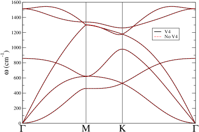
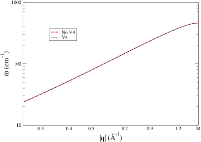
Extended Data Figure 1: Physcial phonons in the static approach with the atomistic potential at $500$ K including and neglecting $\overset{(4)}{\mathbf{\Phi}}$ in Eq. (11). The right panel only includes the ZA modes and it is in logarithmic scale. The calculation is done in a $6\times 6$ supercell.

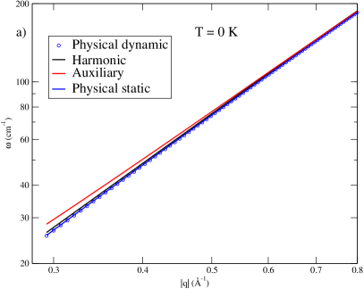
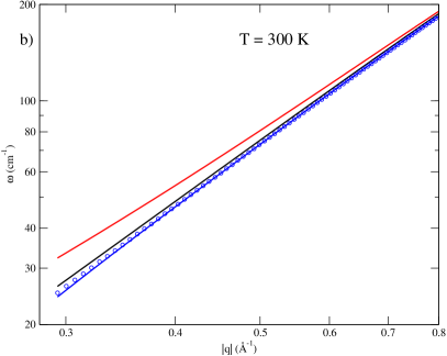
Extended Data Figure 2: Harmonic, and SCHA auxiliary and physical phonons (static and dynamic) calculated at 0 K (a) and 300 K (b) with the atomistic potential for the ZA mode.

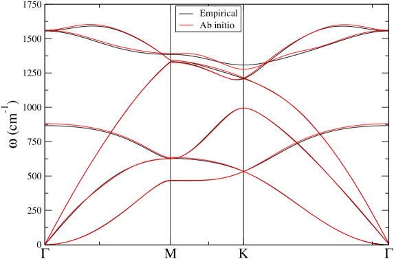
Extended Data Figure 3: Harmonic phonon spectrum of graphene calculated with the machine learning empirical potential and $ab$ $initio$. The calculations are done in a $6\times 6$ supercell.

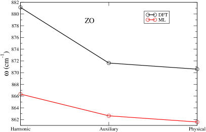
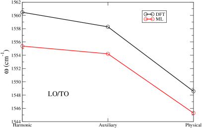
Extended Data Figure 4: Harmonic, and SCHA auxiliary and physical frequencies (static) using the DFT and machine learning (ML) forces. The left panel shows the in-plane optical frequency at the $\Gamma$ point and the right panel the out-of-plane one.

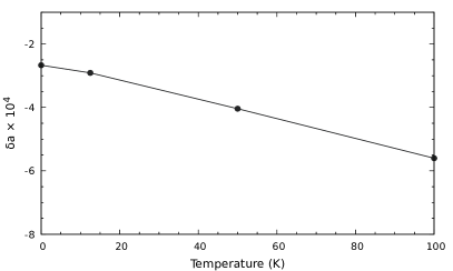
Extended Data Figure 5: $\delta a$ as a function of temperature in the membrane model.

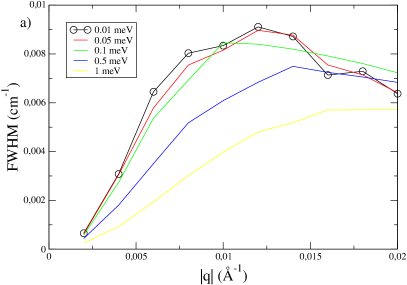
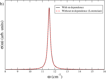
Extended Data Figure 6: (a) Linewidth (full width at half maximum, FWHM) contribution of the term containing the fourth-order tensor of the LA mode calculated in the membrane model at 100 K using the harmonic and SCHA auxiliar phonons. The value of the smearing is in the legend. (b) Spectral function of the LA mode with momentum 0.01 $\AA^{-1}$ with and without considering the frequency dependence of the self energy.

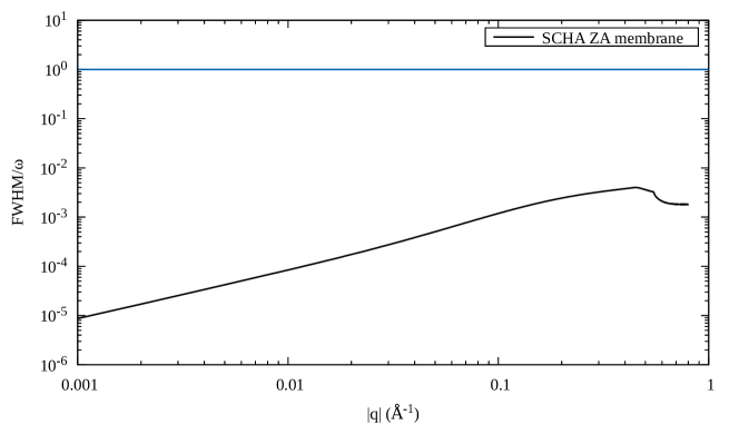
Extended Data Figure 7: Linewidth (full width half maximum) of ZA phonon mode divided by its frequency at 300K calculated within the membrane model.

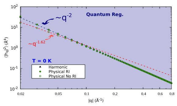
Extended Data Figure 8: Fourier transform of the height-height correlation function at 0 K in the membrane model evaluated at different levels of approximation: harmonic (black dots), anharmonic rotationally invariant (RI) result (green filled dots) and anharmonic no rotationally invariant (No RI) result (green empty dots). The dashed lines correspond to the linear fitting in each case.

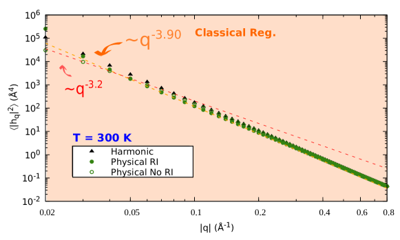
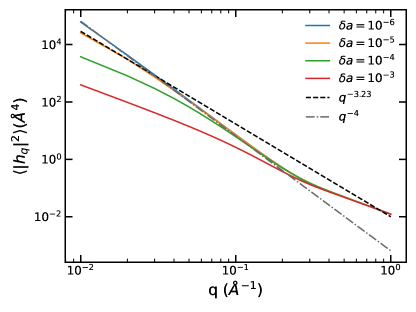
Extended Data Figure 9: Fourier transform of the height-height correlation function at 300 K in the membrane model evaluated at different levels of approximation: harmonic (black dots), anharmonic RI result (green filled dots) and anharmonic No RI result (green empty dots). The dashed lines correspond to the linear fitting in each case.

Extended Data Figure 10: This figure represents the value of $\braket{}{h(\mathbf{q})}{{}^{2}}$ as a function of the biaxial strain $\delta a$. Impressively, the behavior for small $q$ deviates from the $q^{-4}$ law even for very small strains, e.g. $\delta a=10^{-5}$.

References

[1]
L. D. Landau and E. M. Lifshitz.
Statistical Physics.
Pergamon, 1980.
[2]
N David Mermin.
Crystalline order in two dimensions.
Physical Review, 176(1):250, 1968.
[3]
Kostya S Novoselov, Andre K Geim, Sergei V Morozov, D Jiang, Y_ Zhang,
Sergey V Dubonos, Irina V Grigorieva, and Alexandr A Firsov.
Electric field effect in atomically thin carbon films.
science, 306(5696):666–669, 2004.
[4]
Kostya S Novoselov, D Jiang, F Schedin, TJ Booth, VV Khotkevich, SV Morozov,
and Andre K Geim.
Two-dimensional atomic crystals.
Proceedings of the National Academy of Sciences,
102(30):10451–10453, 2005.
[5]
Jannik C. Meyer, A. K. Geim, M. I. Katsnelson, K. S. Novoselov, T. J. Booth,
and S. Roth.
The structure of suspended graphene sheets.
Nature, 446(7131):60–63, 2007.
[6]
Nelson, D.R. and Peliti, L.
Fluctuations in membranes with crystalline and hexatic order.
J. Phys. France, 48(7):1085–1092, 1987.
[7]
A. Fasolino, J. H. Los, and M. I. Katsnelson.
Intrinsic ripples in graphene.
Nature Materials, 6(11):858–861, 2007.
[8]
Doron Gazit.
Correlation between charge inhomogeneities and structure in graphene
and other electronic crystalline membranes.
Phys. Rev. B, 80:161406, Oct 2009.
[9]
Doron Gazit.
Structure of physical crystalline membranes within the
self-consistent screening approximation.
Phys. Rev. E, 80:041117, Oct 2009.
[10]
P. San-Jose, J. González, and F. Guinea.
Electron-induced rippling in graphene.
Phys. Rev. Lett., 106:045502, Jan 2011.
[11]
L L Bonilla and A Carpio.
Ripples in a graphene membrane coupled to glauber spins.
Journal of Statistical Mechanics: Theory and Experiment,
2012(09):P09015, sep 2012.
[12]
Francisco Guinea, Pierre Le Doussal, and Kay Jörg Wiese.
Collective excitations in a large- model for graphene.
Phys. Rev. B, 89:125428, Mar 2014.
[13]
J. González.
Rippling transition from electron-induced condensation of curvature
field in graphene.
Phys. Rev. B, 90:165402, Oct 2014.
[14]
Miguel Ruiz-Garcia, Luis Bonilla, and Antonio Prados.
Ripples in hexagonal lattices of atoms coupled to glauber spins.
Journal of Statistical Mechanics: Theory and Experiment, 2015,
03 2015.
[15]
I. V. Gornyi, V. Yu. Kachorovskii, and A. D. Mirlin.
Rippling and crumpling in disordered free-standing graphene.
Phys. Rev. B, 92:155428, Oct 2015.
[16]
M. Ruiz-García, L. L. Bonilla, and A. Prados.
Stm-driven transition from rippled to buckled graphene in a
spin-membrane model.
Phys. Rev. B, 94:205404, Nov 2016.
[17]
L. L. Bonilla and M. Ruiz-Garcia.
Critical radius and temperature for buckling in graphene.
Phys. Rev. B, 93:115407, Mar 2016.
[18]
I. V. Gornyi, A. P. Dmitriev, A. D. Mirlin, and I. V. Protopopov.
Electron in the field of flexural vibrations of a membrane: Quantum
time, magnetic oscillations, and coherence breaking.
Journal of Experimental and Theoretical Physics,
123(2):322–347, 2016.
[19]
M. Ruiz-Garcia, L. L. Bonilla, and A. Prados.
Bifurcation analysis and phase diagram of a spin-string model with
buckled states.
Phys. Rev. E, 96:062147, Dec 2017.
[20]
Tommaso Cea, Miguel Ruiz-Garcia, Luis Bonilla, and Francisco Guinea.
Large-scale critical behavior of the rippling phase transition for
graphene membranes.
arXiv e-prints, page arXiv:1911.10536, November 2019.
[21]
Tommaso Cea, Miguel Ruiz-Garcia, Luis Bonilla, and Francisco Guinea.
A numerical study of rippling instability driven by the
electron-phonon coupling in finite size graphene membranes.
arXiv e-prints, page arXiv:1911.10510, November 2019.
[22]
Jose Angel Silva-Guillén and Francisco Guinea.
Electron heating and mechanical properties of graphene.
Phys. Rev. B, 101:060102, Feb 2020.
[23]
Lorenzo Paulatto, Francesco Mauri, and Michele Lazzeri.
Anharmonic properties from a generalized third-order ab initio
approach: Theory and applications to graphite and graphene.
Physical Review B, 87(21):214303, 2013.
[24]
Nicola Bonini, Jivtesh Garg, and Nicola Marzari.
Acoustic phonon lifetimes and thermal transport in free-standing and
strained graphene.
Nano letters, 12(6):2673–2678, 2012.
[25]
Hengjia Wang and Murray S Daw.
Anharmonic renormalization of the dispersion of flexural modes in
graphene using atomistic calculations.
Physical Review B, 94(15):155434, 2016.
[26]
JH Los, Mikhail I Katsnelson, OV Yazyev, KV Zakharchenko, and Annalisa
Fasolino.
Scaling properties of flexible membranes from atomistic simulations:
application to graphene.
Physical Review B, 80(12):121405, 2009.
[27]
Mikhail I Katsnelson and Annalisa Fasolino.
Graphene as a prototype crystalline membrane.
Accounts of chemical research, 46(1):97–105, 2013.
[28]
KV Zakharchenko, MI Katsnelson, and Annalisa Fasolino.
Finite temperature lattice properties of graphene beyond the
quasiharmonic approximation.
Physical review letters, 102(4):046808, 2009.
[29]
Eros Mariani and Felix Von Oppen.
Flexural phonons in free-standing graphene.
Physical review letters, 100(7):076801, 2008.
[30]
Bruno Amorim, R Roldán, E Cappelluti, A Fasolino, F Guinea, and
MI Katsnelson.
Thermodynamics of quantum crystalline membranes.
Physical Review B, 89(22):224307, 2014.
[31]
PL De Andres, F Guinea, and MI Katsnelson.
Bending modes, anharmonic effects, and thermal expansion coefficient
in single-layer and multilayer graphene.
Physical Review B, 86(14):144103, 2012.
[32]
K. H. Michel, S. Costamagna, and F. M. Peeters.
Theory of anharmonic phonons in two-dimensional crystals.
Phys. Rev. B, 91:134302, Apr 2015.
[33]
K. H. Michel, P. Scuracchio, and F. M. Peeters.
Sound waves and flexural mode dynamics in two-dimensional crystals.
Phys. Rev. B, 96:094302, Sep 2017.
[34]
Pierre Le Doussal and Leo Radzihovsky.
Self-consistent theory of polymerized membranes.
Phys. Rev. Lett., 69:1209–1212, Aug 1992.
[35]
Melina K. Blees, Arthur W. Barnard, Peter A. Rose, Samantha P. Roberts,
Kathryn L. McGill, Pinshane Y. Huang, Alexander R. Ruyack, Joshua W. Kevek,
Bryce Kobrin, David A. Muller, and Paul L. McEuen.
Graphene kirigami.
Nature, 524(7564):204–207, Aug 2015.
[36]
Niklas Lindahl, Daniel Midtvedt, Johannes Svensson, Oleg A. Nerushev, Niclas
Lindvall, Andreas Isacsson, and Eleanor E. B. Campbell.
Determination of the bending rigidity of graphene via electrostatic
actuation of buckled membranes.
Nano Letters, 12(7):3526–3531, Jul 2012.
[37]
Amjad al Taleb, Gloria Anemone, Daniel Farías, and Rodolfo Miranda.
Acoustic surface phonons of graphene on ni (111).
Carbon, 99:416–422, 2016.
[38]
Amjad Al Taleb, Hak Ki Yu, Gloria Anemone, Daniel Farías, and Alec M
Wodtke.
Helium diffraction and acoustic phonons of graphene grown on copper
foil.
Carbon, 95:731–737, 2015.
[39]
Amjad Al Taleb, Gloria Anemone, Daniel Farías, and Rodolfo Miranda.
Resolving localized phonon modes on graphene/ir (111) by inelastic
atom scattering.
Carbon, 133:31–38, 2018.
[40]
Martin Tømterud, Simen K. Hellner, Sabrina D. Eder, Stiven Forti, Joseph R.
Manson, Camila Colletti, and Bodil Holst.
Temperature dependent bending rigidity of graphene, 2022.
[41]
Raffaello Bianco, Ion Errea, Lorenzo Paulatto, Matteo Calandra, and Francesco
Mauri.
Second-order structural phase transitions, free energy curvature, and
temperature-dependent anharmonic phonons in the self-consistent harmonic
approximation: Theory and stochastic implementation.
Physical Review B, 96(1):014111, 2017.
[42]
Ion Errea, Matteo Calandra, and Francesco Mauri.
Anharmonic free energies and phonon dispersions from the stochastic
self-consistent harmonic approximation: Application to platinum and palladium
hydrides.
Physical Review B, 89(6):064302, 2014.
[43]
Lorenzo Monacelli, Ion Errea, Matteo Calandra, and Francesco Mauri.
Pressure and stress tensor of complex anharmonic crystals within the
stochastic self-consistent harmonic approximation.
Physical Review B, 98(2):024106, 2018.
[44]
Patrick Rowe, Gábor Csányi, Dario Alfè, and Angelos Michaelides.
Development of a machine learning potential for graphene.
Physical Review B, 97(5):054303, 2018.
[45]
Lorenzo Monacelli and Francesco Mauri.
Time-dependent self-consistent harmonic approximation: Anharmonic
nuclear quantum dynamics and time correlation functions.
Phys. Rev. B, 103:104305, Mar 2021.
[46]
Jae-Mo Lihm and Cheol-Hwan Park.
Gaussian time-dependent variational principle for the
finite-temperature anharmonic lattice dynamics.
Phys. Rev. Research, 3:L032017, Jul 2021.
[47]
ZK Wang, HS Lim, SC Ng, B Özyilmaz, and MH Kuok.
Brillouin scattering study of low-frequency bulk acoustic phonons in
multilayer graphene.
Carbon, 46(15):2133–2136, 2008.
[48]
Lev Davidovich Landau and Evgenii Mikhailovich Lifshit’s.
Theory of elasticity.
Theory of elasticity, by Landau, LD; Lifshit’s, EM London,
Pergamon Press; Reading, Mass., Addison-Wesley Pub. Co., 1959. Addison-Wesley
physics books, 1959.
[49]
J.-P. Kownacki and D. Mouhanna.
Crumpling transition and flat phase of polymerized phantom membranes.
Phys. Rev. E, 79:040101, Apr 2009.
[50]
Rafael Roldán, Annalisa Fasolino, Kostyantyn V. Zakharchenko, and Mikhail I.
Katsnelson.
Suppression of anharmonicities in crystalline membranes by external
strain.
Phys. Rev. B, 83:174104, May 2011.
[51]
Juraj Hašík, Erio Tosatti, and Roman
Martoňák.
Quantum and classical ripples in graphene.
Phys. Rev. B, 97:140301, Apr 2018.
[52]
Dongshan Wei and Feng Wang.
Graphene: A partially ordered non-periodic solid.
The Journal of Chemical Physics, 141(14), 10 2014.
144701.
[53]
Max Dion, Henrik Rydberg, Elsebeth Schröder, David C Langreth, and Bengt I
Lundqvist.
Van der waals density functional for general geometries.
Physical review letters, 92(24):246401, 2004.
[54]
John P Perdew, Kieron Burke, and Matthias Ernzerhof.
Generalized gradient approximation made simple.
Physical review letters, 77(18):3865, 1996.
[55]
David Vanderbilt.
Soft self-consistent pseudopotentials in a generalized eigenvalue
formalism.
Physical review B, 41(11):7892, 1990.
[56]
Vincenzo Barone, Maurizio Casarin, Daniel Forrer, Michele Pavone, Mauro Sambi,
and Andrea Vittadini.
Role and effective treatment of dispersive forces in materials:
Polyethylene and graphite crystals as test cases.
Journal of computational chemistry, 30(6):934–939, 2009.
[57]
Hendrik J Monkhorst and James D Pack.
Special points for brillouin-zone integrations.
Physical review B, 13(12):5188, 1976.
[58]
Tjalling J Ypma.
Historical development of the newton–raphson method.
SIAM review, 37(4):531–551, 1995.