Finite size effect on Dissociation and Diffusion of chiral partners in Nambu-Jona-Lasinio model

Abstract

Along with masses of pion and sigma meson modes, their dissociation into quark medium provide a detail spectral structures of the chiral partners. Present article has studied a finite size effect on that detail structure of chiral partners by using the framework of Nambu-Jona-Lasinio model. Through this dissociation mechanism, their diffusions and conductions are also studied. The masses, widths, diffusion coefficients, conductivities of chiral partners are merged at different temperatures in restore phase of chiral symmetry, but merging points of all are shifted in lower temperature, when one introduce finite size effect into the picture. The strengths of diffusions and conductions are also reduced due to finite size consideration.

I Introduction

The nuclear matter, formed in the heavy-ion collision experiments like relativistic heavy ion collider (RHIC) and large hadron collider (LHC), has a finite volume and life time in fm and fm/c scale respectively. Initially a hot quark gluon plasma (QGP) is expected to be form, then it will expand and after a particular volume and time, the medium will freeze out. Experimentally, this freeze out volume can be measured via Hanbury-Brown-Twiss (HBT) methodology, whose details can be found in review articles HBT_rev1 ; HBT_rev2 and references therein. This freeze out volume of the matter depending on the size of the colliding nuclei, center of mass energy and collision centrality RHIC_BES . A freeze out volume range 2000-3000 fm³ within a large range of center of mass energy $\sqrt{s}$ is shown by Ref. HBT_pi . On the other hand, volume range 50-250 fm³ is expected from Refs. UrQMD1 ; UrQMD2 . So it is important to understand different Phenomenological quantities if they have any finite size effect within this uncertain volume range of RHIC or LHC matter.

The effects of finite volume have been addressed by many models such as non-interacting bag model elze , quark-meson (QM) model Braun1 ; Braun2 ; Braun3 ; Braun4 ; Braun5 ; Fraga1 ; Braun6 , Nambu–Jona-Lasinio (NJL) model Hosaka ; Abreu1 ; Elbert1 ; Abreu2 ; Abreu3 ; Abreu4 ; NJLV_2018 ; Abreu_uds , Polyakov loop extended NJL (PNJL) Deb1 ; Sur ; Kinkar1 ; SG1 , Polyakov loop extended linear sigma model (PLSM) Magdy_17 , hadron resonance gas (HRG) Greiner ; Samanta1 ; Xu_PLB ; SG2 ; SG3 ; SG_HRGV_rev ; Deb_HRG , Walecka model Abreu5 ; Casimir etc. All of the model calculations accept that the quark-hadron phase diagram can depend on the volume of the matter. Among the NJL and PNJL model studies Hosaka ; Abreu1 ; Elbert1 ; Abreu2 ; Abreu3 ; Abreu4 ; NJLV_2018 ; Abreu_uds ; Deb1 ; Sur ; Kinkar1 ; SG1 on finite size effect, only Ref. NJLV_2018 have recently studied on finite size effect of meson masses, whose more detail extension might provide a rigorous understanding on the properties of chiral partners - $\pi$ and $\sigma$ mesons. Along with the masses of $\pi$ and $\sigma$ mesons, their dissociation probability into quark medium will give a full spectral details of them. Finite size effect on this detail spectral structure of the chiral partners is not been studied before and present work has attempted this task.

The article is organized as follows. Next in Sec. (II), we have built Formalism part, which carry 3 subsections. First in Sec. (II.1), framework of Nambu-Jona-Lasinio model with finite size is introduce, then in Sec. (II.2), the expression of mesonic masses and decay widths are derived, and at the end of Formalism part, in Sec. (II.3), framework of diffusion and conductivity are constructed for mesonic modes. After addressing formalism part, we have explored the numerical results of masses, decay widths, diffusion coefficients, conductivities of the mesonic modes and their finite size effect. Finally, we have summarized our investigation in Sec. (IV).

II Formalism

II.1 NJL model at finite volume

We consider the framework of the Nambu–Jona-Lasinio (NJL) model hatsuda ; hansen for the description of the coupling between quarks and the chiral condensate in the scalar-pseudo-scalar sector. This model nicely captures the chiral symmetry and its spontaneous breaking physics. We will use a two-flavor model, with a degenerate mass matrix for $u$ and $d$ quarks. The Lagrangian can be written as

$${\cal L} = {\sum_{f=u,d}}{\bar{\Psi}_{f}}\gamma_{\mu}i\partial^{\mu}{\Psi_{f}}-\sum_{f}m_{f}{\bar{\Psi}_{f}}{\Psi_{f}}$$ (1)

$$+ G[\sum_{f}({\bar{\Psi}_{f}}{\Psi_{f}})^{2}+({\bar{\Psi}_{f}}i\gamma_{5}\tau^{a}{\Psi_{f}})^{2}]$$

where $f$ denotes the flavors $u$, $d$ respectively, $m_{f}=m_{u}=m_{d}$, $\tau^{a}$ are $SU_{f}(2)$ Pauli matrices acting in flavor space. As a result of dynamical breaking of chiral symmetry in the NJL model, the chiral condensate $\langle\bar{\Psi}\Psi\rangle$ acquires non-zero vacuum expectation values. The constituent mass as a consequence is given by,

$$M_{f}~{}=~{}m_{f}-2G\sigma_{f}$$ (2)

where $\sigma_{f}\equiv\langle\bar{\Psi}_{f}\Psi_{f}\rangle$ represents the chiral condensate. Its diagrammatic representation is sketched in Fig. (1).

Now in order to implement the effect of finite system sizes, one is ideally supposed to choose the proper boundary conditions : periodic for bosons and anti-periodic for fermions. This in effect leads to a sum of infinite extent over discretized momentum values, $p_{i}=\frac{\pi n_{i}}{R}$, $R$ being the dimension of cubical volume. $n_{i}$ are positive integers with i=x,y,z. This would then imply as lower momentum cut-off $p_{min}=\frac{\pi}{R}=\lambda(\rm say)$. The infinite sum over discrete momentum values will be replaced by integration over continuum momentum variation, albeit with the lower momentum cut-off. This in effect implies that the system volume, $V$ will be regarded as a parameter just like temperature, T and chemical potential, $\mu$ on the same footing. Parametrization will be the same as for zero T, zero $\mu$ and infinite V. Any variation therefore occurring due to any of these parameters will be reflected in $\sigma_{f}$, $\Phi$ etc. and through them in meson spectra.

With these simplifications, the thermodynamic potential thereafter takes the form,

$$\Omega = -{\frac{2N_{c}N_{f}}{(2\pi)^{3}}}\int{\sqrt{p^{2}+M^{2}}}dp$$ (3)

$$- {\frac{2N_{c}N_{f}T}{(2\pi)^{3}}}\int dp(ln(1+exp(-\frac{(E-\mu)}{T}))$$

$$+ ln(1+exp(-\frac{(E+\mu)}{T})))+\frac{(M_{f}-m_{f})}{4G}$$

where, each term bears its usual significance, which can be found in Saumen . The parameters used in eq. (1) are usually fixed to reproduce the mass and decay constant of the pion as well as the chiral condensate. The parameters are given in Table (1).

$m_{u}$	$\Lambda$	$g_{S}\Lambda^{2}$	$|\langle\bar{\Psi}_{u}\Psi_{u}\rangle|^{1\over 3}$	$f_{\pi}$	$m_{\pi}$
$(MeV)$	$(GeV)$	$(GeV^{-}2)$	$(MeV)$	$(MeV)$	$(MeV)$
$5.5$	$0.651$	$5.04$	$251$	$92.3$	$139.3$

Table 1: Parameters of the Fermionic part of the model.

Figure 1: Diagrammatic representation of Gap Eq. (2), which make connection between dressed quark (double solid line) with constituent mass $M_{f}$ and bare quark (single solid line) with current quark mass $m_{f}$

II.2 Mesonic Excitations

Figure 2: Diagrammatic representation of transformation of quark-quark interaction into a effective $\pi$, $\sigma$ meson propagators (double dash line), given in Eq. (4).

The properties of the medium beyond bulk thermodynamic properties can be understood by studying the low-lying mesonic excitations. The masses and decay widths of the mesonic resonances are calculated from the correlations of ${\bar{\psi}}_{f}\Gamma\psi_{f}$ type operators in QCD vacuum. The masses and the spectral functions of pseudo-scalar and scalar mesonic states are interesting because of their close connection with the chiral symmetry breaking and its restoration. The collective excitations, that is, the fluctuation of the mean field around the vacuum, can be handled within the random-phase-approximation (RPA) Saumen . Its schematic Feynman diagram Buballa is shown in Fig. (2), revealing the transformation of quark-quark interaction into a effective mesonic propagators. In this approximation, the retarded correlation function is given by

$$D^{R}_{M}(\omega,\overrightarrow{p})=\frac{2iG}{1-2G\Pi_{M}(\omega,\overrightarrow{p})}$$ (4)

$\Pi_{M}(p^{2})$ is the one loop polarization function for the mesonic channel under consideration,

$$\Pi_{M}(p^{2})=\int{\frac{d^{4}p}{(2\pi)^{4}}}Tr[\Gamma_{M}S({\frac{(q+p)}{2}})\Gamma_{M}({\frac{(q-p)}{2}})]$$ (5)

$S(q)$ is the quark propagator and $\Gamma_{M}$ is the effective vertex factor. The mass of the meson is extracted from the pole of the meson propagator at zero momentum, given by the equation

$$1-2GRe\Pi_{M}(m_{M},\overrightarrow{0})=0$$ (6)

The mass of the unbound resonance has been considered as the real part of $\Pi_{M}$. For bound state solutions $(\omega=m_{M}<2M)$, the polarization function is always real. For $m_{M}>2M$, $\Pi_{M}$ has an imaginary part and the meson spectral function gets a continuum contribution. The meson is no longer a bound state but a resonant one. If $Im\Pi$ stays constant around the position of the peak, the spectral function will be approximated by a Lorentzian with a decay width

$$\gamma_{M}=2GIm\Pi_{M}(m_{M},\overrightarrow{0}).$$ (7)

Explicitly,

$$\Pi_{\pi}(m_{\pi},\overrightarrow{0})=I_{1}-m^{2}_{\pi}I_{2}(m_{\pi},0)$$

$$\Pi_{\sigma}(m_{\sigma},\overrightarrow{0})=I_{1}-(m^{2}_{\sigma}-2M^{2})I_{2}(m_{\sigma})$$ (8)

where

$$I_{1}=\frac{2N_{c}N_{f}}{(2\pi)^{3}}\int\frac{dq}{E_{q}}(1-f_{-}(\overrightarrow{q},\beta,\mu)-f_{+}(\overrightarrow{q},\beta,\mu))$$ (9)

and

$$I_{2}(m_{\pi/\sigma}) = \frac{2N_{c}N_{f}}{(2\pi)^{3}}\int\frac{dq}{E_{q}}(1-f_{-}(q,\beta,\mu)-f_{+}(q,\beta,\mu))$$ (10)

$$~{}~{}~{}~{}~{}~{}~{}~{}\frac{1}{m^{2}_{\pi/\sigma}-4E^{2}}~{}.$$

The masses of the pion and sigma mesons are given, using the gap equation

$${m_{0}\over M+2Gm^{2}_{\pi}ReI_{2}(m_{\pi})}=0$$ (11)

and

$${m_{0}\over M+2G(m_{\sigma}^{2}-4M^{2})ReI_{2}(m_{\sigma})}=0$$ (12)

The real and imaginary part of $\Pi_{M}(\omega,\vec{0})$ are given as

$$Re\Pi_{M}(\omega,\vec{0}) = {\frac{2N_{c}N_{f}}{(2\pi)^{3}}}\int d\vec{q}{\frac{1}{E_{\vec{q}}}}{\frac{{E^{2}_{\vec{q}}}-{\epsilon_{M}}/4}{{E^{2}_{\vec{q}}}-{\omega^{2}/4}}}$$ (13)

$$(1-f_{-}(E_{\vec{q}})-f_{+}(E_{\vec{q}}))$$

$$Im\Pi_{M}(\omega,\vec{0}) = \theta(\omega^{2}-4m^{2}){\frac{N_{c}N_{f}}{8\pi\omega}}(\omega^{2}-\epsilon_{M}^{2})$$ (14)

$$(1-f_{-}(\omega)-f_{+}(\omega))~{}.$$

Here, $f_{\mp}(x)$ is the Fermi distribution function for particles and antiparticles.

II.3 Diffusion of chiral partners

We know that $\pi$ and $\sigma$ meson are pseudo-scalar and scalar modes of same quark condensate with same spin quantum no ($J=0$) but different parity states $\pi=-1,+1$. Particle physicist generally follow the compact notation of Spin and parity quantum no as $J^{\pi}$. So we can visualize that $\pi$ and $\sigma$ meson are basically $J^{\pi}=0^{-1}$ and $0^{+1}$ quantum states of same quark composition. They are called as chiral partners. Quarks are the fundamental building block of hadrons and a non-zero quark condensate is responsible for the mass difference between chiral partners at $T=0$. Now, increasing the temperature of nuclear or hadronic matter, a phase transition from hadrons to quarks can be occurred beyond a transition temperature and corresponding condensate also melts down. Due to this transformations - from non-zero to zero condensate, from breaking to restore phase of chiral symmetry, the mass difference of chiral partners are disappeared. NJL model (as well as other effective QCD models) can nicely capture these facts, whose mathematical framework is already addressed in earlier Secs. (II.1) and (II.2) and results will be discussed in next Sec. (III). In present subsection, we will discuss about the drag, diffusion and conduction of two mesonic modes via dissociations into quarks and anti-quarks. The mathematical anatomy of dissociation process, already addressed in Eq. (14), which can directly be connected with drag and then with diffusion and conduction of chiral partners. Here we will build first the diagrammatic construction of conductivity and diffusion. Then, at the end, we will see the position of drag in the diagrammatic expression of conductivity and diffusion.

Figure 3: (A) One-loop schematic representation of $\pi$ or $\sigma$ meson current-current correlator, whose low frequency limit is connected with their diffusion coefficient or conductivity. (B) Dissociation diagram of $\pi$ or $\sigma$ meson to quark and anti-quark.

In real-time thermal field theory, two point function of meson current ($J_{\mu}\equiv\phi\partial_{\mu}\phi$) can be expressed in a $2\times 2$ matrix structure, which can normally be diagonalized in terms of a single element like retarded component $\Pi^{R}_{\mu\nu}(q_{0},\vec{q})$ or the spectral function $\rho_{\mu\nu}(q_{0},\vec{q})$ of that mesonic correlator. Starting with 11 component ($\Pi^{11}_{\mu\nu}$) of the $2\times 2$ matrix, one can obtain anyone of these quantities by using of their connecting relation:

$$\rho_{\mu\nu}(q_{0},\vec{q}) = 2{\rm Im}\Pi^{R}_{\mu\nu}(q_{0},\vec{q})$$ (15)

$$= 2{\rm tanh}(\frac{\beta q_{0}}{2}){\rm Im}\Pi^{11}_{\mu\nu}(q_{0},\vec{q})~{}.$$

With the help of Wick contraction technique, the 11 component of current-current correlator can be derived as

$$\Pi^{11}_{\mu\nu}(q_{0},\vec{q}) = i\int d^{4}xe^{iqx}\langle TJ_{\mu}(x)J_{\nu}(0)\rangle_{\beta}$$

$$= i\int d^{4}xe^{iqx}\langle T{\phi}\underbrace{(x)\partial_{\mu}{\phi}\overbrace{(x){\phi}}(0)\partial_{\nu}\phi}(0)\rangle_{\beta}$$

$$= i\int\frac{d^{4}k}{(2\pi)^{4}}N_{\mu\nu}(q,k)D_{11}(k)D_{11}(p=q+k)~{},$$

where

$$D^{11}(k)=\frac{-1}{k_{0}^{2}-\omega_{k}^{2}+i\epsilon}+2\pi in_{k}\delta(k_{0}^{2}-\omega_{k}^{2})~{},$$ (17)

where $n_{k}=1/(e^{\beta\omega_{k}}-1)$ is Bose-Einstein (BE) distribution function of meson and

$$N_{\mu\nu}(q,k)=-4k_{\mu}(q-k)_{\nu}~{}.$$ (18)

The Eq. (LABEL:P_11) can diagrammatically be associated with a one-loop kind of self-energy diagram with meson internal lines, shown in Fig. 3(A). Now from this correlator $\Pi^{11}_{\mu\nu}$ one can identify the useful correlators - (1). density-density correlator:

$$\Pi^{R}_{00}(q_{0},\vec{q})=i\int d^{4}xe^{iqx}\langle[J_{0}(x),J_{0}(0)]\rangle_{\beta}$$ (19)

and (2). spatial current-current correlator:

$$\Pi^{R}_{ij}(q_{0},\vec{q})=i\int d^{4}xe^{iqx}\langle[J_{ij}(x),J_{ij}(0)]\rangle_{\beta}~{}.$$ (20)

The spatial current-current correlator can be decomposed in transverse and longitudinal components as

$$\Pi^{R}_{ij}(q_{0},\vec{q})=\left(\frac{q_{i}q_{j}}{q^{2}}-\delta_{ij}\right)\Pi^{R}_{T}(q_{0},\vec{q})+\frac{q_{i}q_{j}}{q^{2}}\Pi^{R}_{L}(q_{0},\vec{q})~{},$$ (21)

where our matter of interest is on longitudinal component $\Pi^{R}_{L}(q_{0},\vec{q})$, which can be extracted from both density-density and (spatial) current-current correlators by using the relation:

$$\Pi^{R}_{L}(q_{0},\vec{q})=\frac{q_{0}^{2}}{q^{2}}\Pi^{R}_{00}(q_{0},\vec{q})=\frac{q^{i}q^{j}}{q^{2}}\Pi^{R}_{ij}(q_{0},\vec{q})~{}.$$ (22)

So we can define a spectral function without Lorentz indices

$$\rho=2\Pi^{R}_{L}(q_{0},\vec{q})~{}.$$ (23)

Using (17) in Eq. (LABEL:P_11) and then using the other Eqs. (15), (23), we get the simplified structure in positive but low $q_{0}$ region

$$\rho(q_{0},\vec{q})=2\int\frac{d^{3}k}{(2\pi)^{3}}\frac{(-\pi)N}{4\omega_{k}\omega_{p}}\{C_{3}\delta(q_{0}+\omega_{k}-\omega_{p})\}$$

$$~{}~{}~{}~{}~{}=2\int\frac{d^{3}k}{(2\pi)^{3}}\frac{N}{4\omega_{k}\omega_{p}}\lim_{\gamma\rightarrow 0}\left[\frac{C_{3}\gamma}{(q_{0}+\omega_{k}-\omega_{p})^{2}+\gamma^{2}}\right]~{},$$

(24)

where $C_{3}\approx q_{0}\beta\{n^{+}_{k}(1-n^{+}_{k})\}$ in the region of $q_{0}<<\omega_{k}$.

We will take finite value of $\gamma$ in our further calculations to get a non-divergent values of pion ($\pi$) and sigma ($\sigma$) meson conductivity

$$\sigma = \frac{1}{6}\lim_{q_{0},\vec{q}\rightarrow 0}\frac{\rho(q_{0},\vec{q})}{q_{0}}$$ (25)

$$= \frac{1}{\gamma}2\beta\int^{\infty}_{0}\frac{d^{3}\vec{k}}{(2\pi)^{3}}\frac{1}{3}\Big{(}\frac{\vec{k}}{\omega_{k}}\Big{)}^{2}[n_{k}\{1+n_{k}\}]$$

where

$$\chi_{s}=2\beta\int^{\infty}_{0}\frac{d^{3}\vec{k}}{(2\pi)^{3}}[n_{k}\{1+n_{k}\}]$$ (26)

is static susceptibility and $\omega_{k}=\{\vec{k}^{2}+m_{\pi,\sigma}^{2}\}^{1/2}$. So identifying $\gamma_{\pi,\sigma}$ as drag coefficient of $\pi$ and $\sigma$ mesons, one can calculate spatial diffusion constant

$$D=\sigma/\chi_{s}$$ (27)

Eq. (24) can be approximated as

$$\sigma=\frac{1}{\gamma}\langle v^{2}/3\rangle\chi_{s}~{},$$ (28)

and then using the further approximated relation $\langle v^{2}/3\rangle=T/m$, based on non-relativistic equipartition theorem, we can easily find Einstein relation

$$\langle v^{2}/3\rangle\frac{1}{\gamma}=\frac{T}{m_{\pi,\sigma}\gamma}=D~{}.$$ (29)

The Eqs. (25) to (29) represent basically general connection among the quantities - $D$, $\gamma$, $\sigma$, $\chi_{s}$. Here our interest on those quantities for $\pi$ and $\sigma$ mesonic condensates, so we can denote them as $D_{\pi,\sigma}$, $\gamma_{\pi,\sigma}$, $\sigma_{\pi,\sigma}$, $\chi^{\pi,\sigma}_{s}$ respectively. Reader can find similar kind of calculation of same quantities for heavy quark in Ref. Teany .

Here, we want to obtain drag ($\gamma_{\pi,\sigma}$), diffusion ($D_{\pi,\sigma}$) coefficients and conductivity ($\sigma_{\pi,\sigma}$) for $\pi$ and $\sigma$ mesons near and beyond Mott temperature, where those mesonic condensates face mostly quarks and anti-quarks in the medium. So, it is via $\pi/\sigma\rightarrow Q+{\bar{Q}}$ decay process, the mesonic condensates will dissipate through medium, whose corresponding $\gamma_{\pi,\sigma}$, $D_{\pi,\sigma}$ and $\sigma_{\pi,\sigma}$ are our matter of interest to estimate. Here, drag coefficients of $\pi,\sigma$ states is estimated through the decay process of $\pi\rightarrow Q{\bar{Q}}$ and $\sigma\rightarrow Q{\bar{Q}}$. Hence we can exactly equate $\gamma_{\pi,\sigma}$ with Eq. (7), which estimate decay probability of $\pi,\sigma\rightarrow Q{\bar{Q}}$ from imaginary part of mesonic self-energy. This dissociation diagrams are sketched in Fig. 3(B). After obtaining the drag coefficients $\gamma_{\pi,\sigma}$, we can calculate $D_{\pi,\sigma}$ and $\sigma_{\pi,\sigma}$ with the help of Eqs.(25), (27).

III Results and discussion

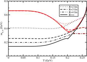
Figure 4: (Color online) $T$ dependence of pion (black) and sigma (red) meson masses for $R=\infty$ (solid line), $4$ fm (dash-dotted line), $3$ fm (dash line) and $2$ fm (dotted line).

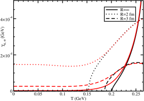
Figure 5: (Color online) $T$ dependence of pion (black) and sigma (red) meson decay widths through quark-anti-quark channel for different system size.

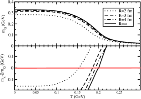
Figure 6: $T$ dependence of (a) $M_{Q}$ and (b) $m_{\pi}-2M_{Q}$ for different system size. Straight horizontal red line, located at $m_{\pi}-2M_{Q}=0$, are indicating corresponding Mott temperature $T_{M}$ for different values of $R$.

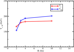
Figure 7: Modification of transition temperature $T_{c}$ and Mott temperature $T_{M}$ for changing system size $R$, where $R=10$ is approximately considered as infinite volume.

In this section we will present the numerical results for the properties of the $\pi$ and $\sigma$ mesons in a hot and dense environment. The masses of the $\pi$ and $\sigma$ mesons are obtained from Eq. (6) and the decay widths can be calculated from Eq. (7).

Fig. (4) shows the temperature dependence of chiral partners $\pi$ and $\sigma$ mesons for different system size $R$. As we know that in our real world (for $T=0$) their masses are well separated but at high temperature they will be in degenerate states. This fact of merging chiral partners is considered as alternative signature of chiral symmetry restoration. This transition from chiral symmetry breaking to restoration is noticed for both infinite and finite system size but their merging pattern become different. At $T=0$, mass of $\pi$ meson enhances as we decrease the system size, while mass of $\sigma$ meson remain unchanged. Actually as the volume decreases, the difference between $\pi$ and $\sigma$ meson also decreases, which indicates that the chiral symmetry effect reduces with decreasing volume. Also $T_{C}$ changes with the volume of the system and shifted to lower temperature for smaller system size.

Next, in Fig. (5), we have plotted $\pi$ and $\sigma$ decay widths in $Q{\bar{Q}}$ channel for different system sizes. Since $\sigma$ meson mass always remain greater than two times of quark mass ($m_{\sigma}>2M_{Q}$) in entire temperature range, therefore we will get non-zero $\gamma_{\sigma}$ in entire $T$. Whereas, for the case of $\pi$ meson mass, the kinematic threshold $m_{\pi}>2M_{Q}$ is valid above the Mott temperature $T_{M}$, below which the $\pi\rightarrow Q{\bar{Q}}$ decay is forbidden. For $R=\infty$ case, $T_{M}=0.201$ GeV and one can find that black solid line, denoting $\gamma_{\pi}$, has started to be non-zero beyond that temperature. Similar to mass merging, the decay width merging of chiral partners are also seen. It is expected as the kinematic phase-space of two decay probabilities depend on their mass only. Their coupling constants are not different as in NJL model, $\pi$ and $\sigma$ meson states are basically considered as condensates of same quark composition but with different spin-parity quantum number $J^{\pi}$ (=$0^{-}$ and $0^{+}$ for $\pi$ and $\sigma$ meson respectively). When we consider finite size effect, we find that the $\gamma_{\sigma}$ is getting enhancement in low $T$ domain. Mott temperature is decreasing as $R$ decreases, which can be seen from shifting threshold pion decay width along $T$-axis.

Fig. 6(a) shows quark masses as a function of $T$ and $R$. Knowing $M_{Q}(T,R)$ and $m_{\pi}(T,R)$, one can find the Mott temperature $T_{M}(R)$ as a function of $R$, where $m_{\pi}-2M_{Q}=0$. It is plotted in Fig. 6(b), from where we get $T_{M}(R)$, which is plotted by red solid line with circles in the Fig. 7. From Fig. 6 one can see that the Mott temperature value decreases for lower system size. The value of the Mott temperature for $R=2fm$ is quite smaller than the higher volume systems.

Fig. 7 represents the variation of the transition temperature and Mott transition temperature with $R$. The transition temperature can be obtained from the maxima of the fist derivative of the chiral condensates for the different finite system size. As $R$ increases both the transition temperature and the Mott transition temperature increases and after $R=4fm$, both the transition temperature and the Mott transition temperature attained saturation. The value of the Mott transition temperature is lower than the transition temperature below $R=3fm$. As we increase the size of the system the Mott temperature value start increasing than the transition temperature and saturates at a higher value than the transition temperature.

Using the $m_{\pi,\sigma}(T,R)$ and $\gamma_{\pi,\sigma}(T,R)$ in Eq. (25), we have obtained the conductivity of the pion and sigma $\sigma_{\pi,\sigma}(T,R)$, which is plotted in Fig. (8). Below the Mott temperature, the divergence nature of $\sigma_{\pi}(T,R)$ can be clearly seen due to the relation $\sigma_{\pi}\propto 1/\gamma_{\pi}$. The conductivity of the pion and sigma meson changes significantly with the variation of the system size and decreases with the decreasing volume. The conductivity of pion and sigma meson merges after the transition temperature. For lower system size the conductivity decreases with the decreasing transition temperature and so the pion and sigma meson merges at a lower value.

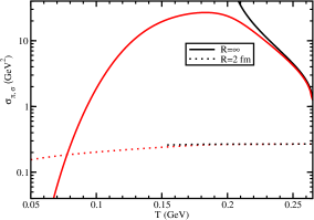
Figure 8: (Color online) Conductivity of $\pi$ (black) and $\sigma$ (red) mesons or light flavor condensates with quantum number $J^{\pi}=0^{-}$ and $0^{+}$ for $R=\infty$ (solid line) and $2$ fm (dotted line).

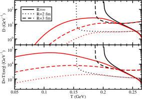
Figure 9: (Color online) Diffusion coefficients $D$ of $\pi$ (black) and $\sigma$ (red) mesons or light flavor condensates with quantum number $J^{\pi}=0^{-}$ and $0^{+}$ for $R=\infty$ (solid line), $3$ fm (dash line) and $2$ fm (dotted line).

Table 2: Transition temperature ($2^{nd}$ column), Mott temperature ($3^{rd}$ column), Temperatures, where masses ($4^{th}$ column), drag coefficients ($2^{nd}$ column), diffusion coefficients ($3^{rd}$ column) and conductivity ($4^{th}$ column) of chiral partners are merged for $R=\infty$ ($2^{nd}$ and $5^{th}$ rows) and $R=2$ fm ($3^{rd}$ and $6^{th}$ rows), temperatures are in MeV.

Size	Transition	Mott	Mass
	Temperature	Temperature	Doublet
$R=\infty$	184	200	245
$R=2$ fm	166	153	223
Size	Drag	Diffusion	Conductivity
	Doublet	Doublet	Doublet
$R=\infty$	234	245	236
$R=2$ fm	188	195	193

Fig.9(a) shows the diffusion coefficients of $\pi$ and $\sigma$ mesons by using Eq. (27), while Fig.9(b) shows corresponding results by using Einstein relation, given in Eq. (29). Here also, one can notice the divergence nature of $D_{\pi}(T,R)$ below the Mott temperature and realize the responsible relation $D_{\pi}\propto 1/\gamma_{\pi}$.

At the end, if we briefly take a look on all the quantities of chiral partners for infinite ($R=\infty$) and finite ($R=2$ fm) sizes of medium, then we can get a table, given in (2). It clearly implies that transition temperature, Mott temperature are shifted in lower temperature when we go from infinite to finite matter. Table (2) has also documented the temperatures, where masses ($4^{th}$ column), drag coefficients ($2^{nd}$ column), diffusion coefficients ($3^{rd}$ column) and conductivity ($4^{th}$ column) of $\pi$ and $\sigma$ mesons are merged. Similar to chiral condensate melting, forming mass doublets beyond the transition temperature is an alternative realization of chiral symmetry restoration. In that regard, merging of other quantities like drag, diffusion coefficients, conductivity might also be considered as alternative realization chiral symmetry restoration. In fact, collection all quantities provide a rich understanding on the different thermodynamical properties of chiral partners and transition details from breaking to restore phase of chiral symmetry. Transition point with respect to the drag, diffusion coefficients, conductivity will also be shifted in lower temperature, when one goes from infinite to finite size matter.

IV Summary

We have studied the finite volume effect on the spectral functions of strongly interacting matter at zero chemical potential. We have shown the pion and sigma meson masses and decay widths at different finite system sizes. Also, we have calculated the conductivity and diffusion coefficients of pion and sigma mesons. All the quantities have shown the significant variation with the finite system size.

At low temperature the chiral symmetry is broken and after the transition temperature the chiral symmetry is restored. The transition from the chiral symmetry broken phase to the chiral symmetry restored phase can be visualized in both infinite volume system and the finite volume system. Based on the quark condensate or quark mass melting, we can define an chiral transition temperature, which is shifting to lower values when we go from infinite to finite size matter. An alternative chiral symmetry restoration can be realized from merging of $\pi$ and $\sigma$ masses near and after the transition temperature. This merging point is also shifting towards lower temperature due to finite size consideration.

We have shown the decay widths of the pion and sigma meson masses with different system size. Decay widths are basically estimated from the imaginary part of self-energy for pion and sigma meson, which interpret the thermodynamical probabilities of their dissociation to quark, anti-quark channels. For the sigma meson, the decay width can be seen for the entire temperature range. However for the pion, the decay width starts after the Mott transition temperature, which also decreases with decreasing system size. Similar to masses of the chiral partners, their the decay widths also merge in the temperature domain of restored phase. Again the finite size consideration make their merging points shift towards lower values of temperature. For finite size effect, we find that the decay width of $\sigma$ meson is getting enhancement in low $T$ domain, which is quite interesting and new outcome.

Considering the dissociation process as dragging mechanism of $\pi$, $\sigma$ modes with medium, we have estimated their diffusion coefficients and conductivities. Low temperature $\pi$ mode diffusion or conduction is diverged due to vanishing drag process below the Mott temperature but its non-divergent values beyond Mott temperature are merged latter with corresponding quantities of $\sigma$. Similar to merging of masses and decay widths of chiral partners, their merging of diffusion and conduction values can be considered as alternative realization of restored phase and their merging points again shift towards the low temperature direction when size of the matter is reduced.

Acknowledgment: PD thanks to WoSA scheme of DST funding with grant no….

References

- (1) D. H. Boal, C.-K. Gelbke, and B. K. Jennings, Rev. Mod. Phys. 62, 553 (1990).
- (2) M. A. Lisa, S. Pratt, R. Soltz, and U. Wiedemann, Annu. Rev. Nucl. Part. Sci. 55, 357 (2005).
- (3) Adamczyk L et al (STAR Collaboration), Phys. Rev. C 96 (2017) 044904
- (4) D. Adamova et al., Phys. Rev. Lett. 90, 022301 (2003).
- (5) G. Graef, M. Bleicher, and Q. Li, Phys. Rev. C 85, 044901 (2012).
- (6) S. Bass et al., Prog. Part. Nucl. Phys. 41, 255 (1998).
- (7) H. T. Elze and W. Greiner, Phys. Lett. B 179, 385 (1986).
- (8) J. Braun, B. Klein and B. -J. Schaefer, On the Phase Structure of QCD in a Finite Volume, Phys. Lett. B 713, 216 (2012).
- (9) J. Braun, B. Klein and P. Piasecki, On the scaling behavior of the chiral phase transition in QCD in finite and infinite volume, Eur. Phys. J. C 71, 1576 (2011).
- (10) J. Braun, B. Klein, and H. J. Pirner, Phys. Rev. D 71, 014032 (2005), arXiv:hep-ph/0408116 [hep-ph].
- (11) J. Braun, B. Klein, and H. J. Pirner, Phys. Rev. D 72, 034017 (2005), arXiv:hep-ph/0504127 [hep-ph].
- (12) J. Braun, B. Klein, H. J. Pirner, and A. H. Rezaeian, Phys. Rev. D73, 074010 (2006), arXiv:hep-ph/0512274 [hep-ph].
- (13) L. F. Palhares, E. S. Fraga, and T. Kodama, J. Phys. G 38, 085101 (2011), arXiv:0904.4830 [nucl-th].
- (14) R.-A. Tripolt, J. Braun, B. Klein, and B.-J. Schaefer, Phys. Rev. D90, 054012 (2014).
- (15) O. Kiriyama and A. Hosaka, Chiral phase properties of finite size quark droplets in the Nambu-Jona-Lasinio model, Phys. Rev. D 67, 085010 (2003).
- (16) L. M. Abreu, M. Gomes and A. J. da Silva, Finite-size effects on the phase structure of the Nambu-Jona-Lasinio model, Phys. Lett. B 642, 551 (2006).
- (17) D. Ebert and K. G. Klimenko, Phys. Rev. D 82, 025018 (2010)
- (18) L. M. Abreu, A. P. C. Malbouisson, J. M. C. Malbouisson, and A. E. Santana, Nucl. Phys. B 819, 127 (2009), arXiv:0909.5105 [hep-th].
- (19) L. M. Abreu, A. P. C. Malbouisson and J. M. C. Malbouisson, Finite-size effects on the phase diagram of difermion condensates in two-dimensional four-fermion interaction models, Phys. Rev. D 83, 025001 (2011).
- (20) L. M. Abreu, A. P. C. Malbouisson and J. M. C. Malbouisson, Nambu-Jona-Lasinio model in a magnetic background: Size-dependent effects, Phys. Rev. D 84, 065036 (2011).
- (21) Z. Ya-Peng, Y. Pei-Lin, Y. Zhen-Hua, Z. Hong-Shi Finite volume effects on chiral phase transition and pseudoscalar mesons properties from the Polyakov-Nambu-Jona-Lasinio model, arXiv:1812.09665 [hep-ph].
- (22) L.M. Abreu, C. A. Linhares, A. P.C. Malbouisson( Finite-volume and magnetic effects on the phase structure of the three-flavor Nambu–Jona-Lasinio model, Phys. Rev. D 99 (2019) 076001.
- (23) A. Bhattacharyya, P. Deb, S. K. Ghosh, R. Ray and S. Sur, Thermodynamic Properties of Strongly Interacting Matter in Finite Volume using Polyakov-Nambu-Jona-Lasinio Model, Phys. Rev. D 87, no. 5, 054009 (2013).
- (24) A. Bhattacharyya, R. Ray, S. Sur, Fluctuation of strongly interacting matter in Polyakov Nambu Jona-Lasinio model in finite volume, Phys. Rev. D 91, 051501 (2015).
- (25) A. Bhattacharyya, S. K. Ghosh, R. Ray, K. Saha, and S. Upadhaya, EPL 116, 52001 (2016), arXiv:1507.08795 [hep-ph].
- (26) K. Saha, S. Ghosh, S. Upadhaya, and S. Maity, Phys. Rev. D 97, 116020 (2018), arXiv:1711.10169 [nucl-th].
- (27) N. Magdy, M. Csanad, R. A. Lacey, Influence of finite volume and magnetic field effects on the QCDphase diagram J. Phys. G44, 025101 (2017), arXiv:1510.04380 [nucl-th].
- (28) C. Spieles, H. Stoecker and C. Greiner, Phase transition of a finite quark gluon plasma, Phys. Rev. C 57, 908 (1998).
- (29) A. Bhattacharyya, R. Ray, S. Samanta, and S. Sur, Phys. Rev. C91, 041901 (2015), arXiv:1502.00889 [hep- ph].
- (30) H.-j. Xu, Phys. Lett. B765, 188 (2017), arXiv:1612.06485 [nucl-th].
- (31) S. Samanta, S. Ghosh, and B. Mohanty, J. Phys. G45, 075101 (2018), arXiv:1706.07709 [hep-ph].
- (32) S. Ghosh, S. Samanta, S. Ghosh, H. Mishra, Viscosity calculations from Hadron Resonance Gas model: Finite size effect, Int. J. Mod. Phys. E 28 (2019) 1950036.
- (33) S. Ghosh, S. Ghosh, S. Bhattacharyya, Phenomenological bound on the viscosity of the hadron resonance gas, Phys. Rev. C 98 (2018) 045202.
- (34) N. Sarkar, P. Deb, P. Ghosh, Finite size effect on thermodynamics of hadron gas in high-multiplicity events ofproton-proton collisions at the LHC, arXiv:1905.06532 [hep-ph].
- (35) L. M. Abreu and E. S. Nery, Phys. Rev. C96, 055204 (2017), arXiv:1711.07934 [nucl-th].
- (36) T. Ishikawa, K. Nakayama, K. Suzuki, Casimir effect for nucleon parity doublets, Phys. Rev. D 99 (2019) 054010.
- (37) T. Hatsua and T. Kunihiro, Phys. Rep. bf 247, 221 (1994).
- (38) P. Deb, A. Bhattacharyya, S. Datta, and S. K. Ghosh, Phys. Rev. C 79, 055208 (2009).
- (39) H. Hansen, W. M. Alberico, A. Beraudo, A. Molinari, M. Nardi and C. Ratti, Phys. Rev. D 75 065004 (2007).
- (40) M. Buballa, Phys. Rep. 407, 205 (2005).
- (41) K. Redlich and K. Zalewski, Finite volume corrections and low momentum cuts in the thermodynamics of quantum gases, arXiv:1611.03746 [nucl-th].
- (42) F. Karsch, K. Morita, K. Redlich, Phys. Rev. C 93, 034907 (2016).
- (43) P. Petreczky, D. Teaney, Heavy Quark Diffusion from the Lattice Phys. Rev. D 73 (2006) 014508.