On the stability of harmonic mortar methods with application to electric machines

Abstract

Harmonic stator-rotor coupling offers a promising approach for the interconnection of rotating subsystems in the simulation of electric machines. This paper studies the stability of discretization schemes based on harmonic coupling in the framework of mortar methods for Poisson-like problems. A general criterion is derived that allows to ensure the relevant inf-sup stability condition for a variety of specific discretization approaches, including finite-element methods and isogeometric analysis with harmonic mortar coupling. The validity and sharpness of the theoretical results is demonstrated by numerical tests.

1 Introduction

Electric drives naturally consist of different subdomains, i.e. the stator and rotor, which move relative to each other. The time-varying geometry and nonlinearities caused by saturation effects formally require a time-domain analysis, which is often realized by solving a sequence of quasi-stationary problems at different working points. Several strategies have been proposed for the simulation of the corresponding equations of magnetostatics and, in particular, for the coupling of the fields across the air gap between stator and rotor. As it is common practice, see e.g. DeGersem04 ; Gyselinck03 ; Lange10 , we consider a two dimensional regime, in which the unknown fields are described by the axial component of the magnetic vector potential. The governing system then consists of two Poisson-like problems for the stator and the rotor, which can be coupled via Lagrange multipliers. Such domain decompositions of mortar methods, which couple subdomains via Lagrange multipliers, have been investigated intensively in the literature BenBelgacem99 ; Bernardi94 ; Braess99 ; Wohlmuth00 ; see Buffa01 ; DeGersem04 for results concerning electric machines. It is well-known that a careful choice of approximation spaces is required to obtain stable disretization schemes for underlying saddlepoint problems Brezzi74 ; Raviart77 ; appropriate stabilization Hansbo05 could be used as an alternative approach.

In this paper, we investigate the stability of mortar discretizations using harmonic functions for the stator-rotor coupling DeGersem04 ; Bontinck18 . We discuss in detail the discrete inf-sup condition which is necessary and sufficient to guarantee the stability of such approximations. We provide a simple criterion for the maximal number of harmonics used as Lagrange multipliers depending on the mesh size and polynomial degree of the subdomain discretizations which guarantees the stability of the scheme. Our analysis applies to the harmonic coupling of various discretization methods, e.g., obtained by isogeometric analysis (IGA) Hughes_2005aa ; Bontinck18 ; Brivadis15 , and can in principle be extended to other Lagrange multiplier spaces.

The remainder of this note is organized as follows: In Section 2, we introduce the model problem to be considered and we summarize some well-known results about its analysis and discretization. In Section 3, we then turn to the harmonic stator-rotor coupling, and we state and prove our main results. Section 4 is concerned with numerical tests, in which we demonstrate the validity of our stability criterion for low and high order discretizations based on IGA.

2 Model problem

We consider a typical geometric setup that consists of two subdomains $\Omega_{1}$, $\Omega_{2}$ representing, respectively, the stator and rotor, separated by a small air gap which contains the interface $\Gamma=\partial\Omega_{1}\cap\partial\Omega_{2}$; see Figure 1. Let $\Sigma_{\ell}=\partial\Omega_{\ell}\setminus\Gamma$, $\ell=1,2$, be the remaining parts of the subdomain boundaries and $f_{\ell}=f|_{\Omega_{\ell}}$ denote the restriction of a function $f$ defined on $\Omega_{1}\cup\Omega_{2}$ to the subdomain $\Omega_{\ell}$. We then consider the following elliptic interface problem: Inside the two subdomains, we require

$$-\operatorname{div}(\nu_{\ell}\nabla u_{\ell}) =j_{\ell},\qquad \text{in }\Omega_{\ell},$$ (1)

$$u_{\ell} =0,\qquad \text{on }\Sigma_{\ell},$$ (2)

where $u$ denotes the $z$-component of the magnetic vector potential, $\nu$ the magnetic reluctivity, and $j=j_{s}+\operatorname{div}m^{\perp}$ a generalized current density with $j_{s}$ denoting the $z$-component of the source currents and $m^{\perp}=(m_{y},-m_{x})$ the rotated magnetization vector. The corresponding in-plane components of the magnetic flux density and field strength are given by $b=(\partial_{y}u,-\partial_{x}u)=\nabla^{\perp}u$ and $h=\nu b$, respectively. The coupling of the fields across the interface $\Gamma$ is accomplished by the conditions

$$u_{1} =u_{2},\qquad \text{on }\Gamma,$$ (3)

$$n\cdot(\nu_{1}\nabla u_{1}) =n\cdot(\nu_{2}\nabla u_{2}),\qquad \text{on }\Gamma,$$ (4)

which express the normal continuity of $b$ and the tangential continuity of $h$, respectively.

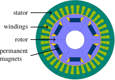
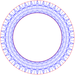
Figure 1: Typical structure of a 6-pole permanent magnet synchronous machine (left) and the coarsest mesh of the stator domain as used in our numerical tests (right).

Here $n=n_{2}$ is the unit normal vector at $\Gamma$ pointing from $\Omega_{2}$ to $\Omega_{1}$. Without further noting, we assume that $\Omega_{\ell}$ are bounded domains with smooth boundaries $\Sigma_{\ell}$ and $\Gamma$, having non-zero measure, and that $\nu$ is bounded from above and below by positive constants $\underline{\nu}$, $\overline{\nu}$, i.e., $\underline{\nu}\leq\nu(x)\leq\overline{\nu}$ for all $x\in\Omega_{1}\cup\Omega_{2}$.

The weak formulation of the interface problem (1)–(4) then reads as follows: Find $u\in V=\{v\in H^{1}(\Omega_{1}\cup\Omega_{2}):v|_{\Sigma_{\ell}}=0\}$ and $\lambda\in M=H^{-1/2}(\Gamma)$ such that

$$(\nu\nabla u,\nabla v)_{\Omega_{1}\cup\Omega_{2}}+\langle\lambda,[v]\rangle_{\Gamma} =\langle j,v\rangle_{\Omega_{1}\cup\Omega_{2}}\qquad \forall v\in V,$$ (5)

$$\langle[u],\mu\rangle_{\Gamma} =0\qquad \forall\mu\in M.$$ (6)

Here $(a,b)_{\Omega_{1}\cup\Omega_{2}}=\int_{\Omega_{1}}a\cdot b\,dx+\int_{\Omega_{2}}a\cdot b\,dx$ is the usual scalar product of functions $a,b\in L^{2}(\Omega_{1}\cup\Omega_{2})$, while $\langle a,b\rangle_{\Omega_{1}\cup\Omega_{2}}$ and $\langle a,b\rangle_{\Gamma}$ are the duality products on $V\times V^{\prime}$ and $M\times M^{\prime}$, respectively, with $V^{\prime}$, $M^{\prime}$ denoting the dual spaces of $V$ and $M$. Furthermore, $H^{1}(\Omega_{1}\cup\Omega_{2})$ denotes the space of piecewise smooth functions $v$ with restrictions $v_{\ell}=v|_{\Omega_{\ell}}\in H^{1}(\Omega_{\ell})$ for $\ell=1,2$ and $[v]=v_{1}-v_{2}$ denotes the jump of such functions across the interface $\Gamma$. Under the above assumptions, we have

Lemma 1

For any $j_{s}\in L^{2}(\Omega)$ and $m\in L^{2}(\Omega)^{2}$, the variational problem (5)–(6) with $j=j_{s}+\operatorname{div}m^{\perp}$ has a unique solution $(u,\lambda)\in V\times M$ and there holds

$$\|u\|_{H^{1}(\Omega_{1}\cup\Omega_{2})}+\|\lambda\|_{H^{-1/2}(\Gamma)}\leq C\big{(}\|j_{s}\|_{L^{2}(\Omega_{1}\cup\Omega_{2})}+\|m\|_{L^{2}(\Omega_{1}\cup\Omega_{2})}).$$

Moreover, $u$ is the unique weak solution of (1)–(4) and $\lambda=n\cdot(\nu\nabla u_{\ell})$ the associated tangential component of the magnetic field strength $h$ at the interface.

Remark 1

The result is well-known and a similar assertion can already be found in the work of Babuska Babuska73 . Using Brezzi’s theory for saddlepoint problems Brezzi74 , the essential ingredient turns out to be the inf-sup stability condition

$$\sup_{v\in V}\frac{\langle\mu,[v]\rangle_{\Gamma}}{\|v\|_{H^{1}(\Omega_{1}\cup\Omega_{2})}}\geq\beta\|\mu\|_{H^{-1/2}(\Gamma)}$$ (7)

which has to hold for all $\mu\in M$ with a uniform constant $\beta>0$. Following Raviart77 , condition (7) can be proven as follows: Let $z_{1}\in H^{1}(\Omega_{1})$ be the weak solution of the mixed boundary value problem

$$-\Delta z_{1}=0\quad\text{in }\Omega_{1}\quad\text{with}\quad z_{1}=0\quad\text{on }\Sigma_{1}\quad\text{and}\quad\partial_{n}z_{1}=\mu\quad\text{on }\Gamma.$$ (8)

Then by standard arguments for elliptic problems Babuska73 ; BenBelgacem99 , one can show that

$$\|z_{1}\|_{H^{1}(\Omega_{1})}\leq c_{2}\|\mu\|_{H^{-1/2}(\Gamma)}\quad\text{and}\quad\langle\mu,z_{1}\rangle_{\Gamma}\geq c_{1}\|\mu\|_{H^{-1/2}(\Gamma)}^{2},$$

with positive constants $c_{1}$, $c_{2}$ only depending on $\Omega_{1}$, $\Sigma_{1}$, and $\Gamma$.
Now define $z\in H^{1}(\Omega_{1}\cup\Omega_{2})$ by $z=z_{1}$ on $\Omega_{1}$ and $z=0$ on $\Omega_{2}$. Then

$$\langle\mu,[z]\rangle_{\Gamma}=\langle\mu,z_{1}\rangle_{\Gamma}\geq c_{1}\|\mu\|^{2}_{H^{-1/2}(\Gamma)}\geq\frac{c_{1}}{c_{2}}\|\mu\|_{H^{-1/2}(\Gamma)}\|z_{1}\|_{H^{1}(\Omega_{1})}.$$

The result now follows with $\beta=\frac{c_{1}}{c_{2}}$ by noting that $\|z\|_{H^{1}(\Omega_{1}\cup\Omega_{2})}=\|z_{1}\|_{H^{1}(\Omega_{1})}$. ∎

Discretization. As a next step, we now consider Galerkin approximations of the weak formulation (5)–(6): Find $u_{h}\in V_{h}\subset V$ and $\lambda_{N}\in M_{N}\subset M$ such that

$$(\nu\nabla u_{h},\nabla v_{h})_{\Omega_{1}\cup\Omega_{2}}+\langle\lambda_{N},[v_{h}]\rangle_{\Gamma} =\langle j,v_{h}\rangle_{\Omega_{1}\cup\Omega_{2}}\qquad \forall v_{h}\in V_{h},$$ (9)

$$\langle[u_{h}],\mu_{N}\rangle_{\Gamma} =0\qquad \forall\mu_{N}\in M_{N}.$$ (10)

The subspaces $V_{h}$, $M_{N}$ are always assumed to be finite dimensional in the following.

Lemma 2

Let the conditions of Lemma 1 be valid and assume that

$$\sup_{v_{h}\in V_{h}}\frac{\langle\mu_{N},[v_{h}]\rangle_{\Gamma}}{\|v_{h}\|_{H^{1}(\Omega_{1}\cup\Omega_{2})}}\geq\beta^{\prime}\|\mu_{N}\|_{H^{-1/2}(\Gamma)}$$ (11)

for all $\mu_{N}\in M_{N}$ with some constant $\beta^{\prime}>0$. Then the variational problem (9)–(10) has a unique solution $u_{h}\in V_{h}$, $\lambda_{N}\in M_{N}$. Furthermore

$$\|u-u_{h} \|_{H^{1}(\Omega_{1}\cup\Omega_{2})}+\|\lambda-\lambda_{N}\|_{H^{-1/2}(\Gamma)}$$ (12)

$$\leq C\,\big{(}\inf_{v_{h}\in V_{h}}\|u-v_{h}\|_{H^{1}(\Omega_{1}\cup\Omega_{2})}+\inf_{\mu_{N}\in M_{N}}\|\lambda-\mu_{N}\|_{H^{-1/2(\Gamma)}}\big{)}$$

with $C$ depending only on $\beta^{\prime}$ in condition (11), the bounds for $\nu$ and the geometry.

Remark 2

The conditions required for the proof of the corresponding result on the continuous level, except the inf-sup stability condition, are inherited by the Galerkin approximation. The existence of a unique solution can thus again be deduced from Brezzi’s saddlepoint theory Brezzi74 . The error estimate (12) follows from Galerkin orthogonality and standard arguments; we refer to Braess99 ; Brezzi74 for details. Hence any choice of approximation spaces $V_{h}$, $M_{N}$ that allows to prove the discrete inf-sup stability condition (11) will lead to a stable discretization with quasi-optimal error estimates.

3 Harmonic stator-rotor coupling

We now consider a particular class of Galerkin approximations (9)–(10) in which $V_{h}$ is constructed by piecewise polynomials, while the Lagrange multiplier space $M_{N}$ is defined by trigonometric polynomials. Our analysis in particular also covers the harmonic-coupling of the methods considered in Bontinck18 ; DeGersem04 .

Using polar coordinates, the computational domain $\Omega=\Omega_{1}\cup\Omega_{2}$ can be represented as the image of a rectangle $\widehat{\Omega}$ under a mapping $F:\widehat{\Omega}\to\Omega$; see Figure 2.

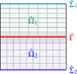
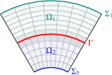
Figure 2: Sketch of a subset of the rectangular reference domain $\hat{\Omega}$ and its mesh (left) and the physical domain $\Omega=F(\hat{\Omega})$ and mesh obtained after mapping. The boundaries on the left and right are only introduced for the illustration but not present in our application.

Now let $\widehat{T}_{h}$ denote a shape-regular partition of $\widehat{\Omega}_{1}\cup\widehat{\Omega}_{2}$ into triangles and/or rectangles of size $h$. The meshes of the two sub-domains are assumed to be geometrically conforming, but they may be non-matching across the interface. We denote by $P_{k}(\widehat{T}_{h})$ the space of piecewise polynomials over $\widehat{T}_{h}$ of degree $\leq k$ and by $\widehat{M}_{N}=\operatorname{span}\{\sin(n\pi\xi),\cos(n\pi\xi):0\leq n\leq N\}$ the spaces of trigonometric polynomials of degree $\leq N$. We then choose the approximation spaces $V_{h}$, $M_{N}$ s.t.

$$M_{N}=F(\widehat{M}_{N})\qquad\text{and}\qquad V_{h}=V_{h}|_{\Omega_{1}}\cup V_{h}|_{\Omega_{2}}\subset F(P^{k}(T_{h}))\cap V.$$ (13)

By the condition $V_{h}=V_{h}|_{\Omega_{1}}\cup V_{h}|_{\Omega_{2}}$ we mean that discrete functions, when restricted to one of the sub-domains and extended by zero to the other still belong to the approximation space $V_{h}$. The basic assumption for the discrete inf-sup stability condition (7) of the corresponding Galerkin approximation (9)–(10) is the following.

Theorem 3.1

Assume that there exists a linear operator $\Pi_{h}:V|_{\Omega_{1}}\to V_{h}|_{\Omega_{1}}$ such that

$$\|\Pi_{h}v_{1}\|_{H^{1}(\Omega_{1})} \leq c_{3}\|v_{1}\|_{H^{1}(\Omega_{1})},$$ (14)

$$\Pi_{h}v_{1} =\pi_{h}v_{1}\quad\text{on }\Gamma,$$ (15)

$$\|v-\pi_{h}v\|_{H^{-1/2}(\Gamma)} \leq c_{4}\tfrac{h}{k}\|v\|_{H^{1/2}(\Gamma)},$$ (16)

where $\pi_{h}:L^{2}(\Gamma)\to V_{h}|_{\Omega_{1}\cap\Gamma}$ denotes the $L^{2}$-projection on $\Gamma$. Then there exists a constant $0<\epsilon<1$, depending only on $c_{3}$, $c_{4}$ in (14)–(16), such that the discrete inf-sup condition (11) holds with $\beta^{\prime}=\beta^{\prime}(\epsilon)$ whenever $N$ and $h$ are chosen such that

$$Nh/k\leq 1-\epsilon.$$ (17)

Proof

As an immediate consequence of the continuous inf-sup condition (7), we can find for $\mu=\pi_{h}\lambda_{N}$ a function $z\in V$ with $z=0$ on $\Omega_{2}$, such that

$$\langle\pi_{h}\lambda_{N},[z]\rangle_{\Gamma}\geq\beta\|z\|_{H^{1}(\Omega_{1}\cup\Omega_{2})}\|\pi_{h}\lambda_{N}\|_{H^{-1/2}(\Gamma)}.$$

We then define $z_{h}=\Pi_{h}z_{1}$ on $\Omega_{1}$ and $z_{h}=0$ on $\Omega_{2}$, and observe that

$$\langle\pi_{h}\lambda_{N},[z_{h}]\rangle_{\Gamma} =\langle\pi_{h}\lambda_{N},[\Pi_{h}z]\rangle_{\Gamma}=\langle\pi_{h}\lambda_{N},\pi_{h}[z]\rangle_{\Gamma}=\langle\pi_{h}\lambda_{N},[z]\rangle_{\Gamma},$$

where we used property (15) and the orthogonality of the $L^{2}$-projection $\pi_{h}$. Together with the previous estimate and employing condition (14), we thus obtain

$$\langle\pi_{h}\lambda_{N},[z_{h}]\rangle_{\Gamma} \geq\beta\|z\|_{H^{1}(\Omega_{1}\cup\Omega_{2})}\|\pi_{h}\lambda_{N}\|_{H^{-1/2}(\Gamma)}\geq\frac{\beta}{c_{3}}\|z_{h}\|_{H^{1}(\Omega_{1}\cup\Omega_{2})}\|\pi_{h}\lambda_{N}\|_{H^{-1/2}(\Gamma)}.$$

Using the triangle inequality, we can further estimate

$$\|\pi_{h}\lambda_{N}\|_{H^{-1/2}(\Gamma)}\geq\|\lambda_{N}\|_{H^{-1/2}(\Gamma)}-\|\lambda_{N}-\pi_{h}\lambda_{N}\|_{H^{-1/2}(\Gamma)},$$

and the last term can be bounded with the approximation error estimate (16) by

$$\|\lambda_{N}-\pi_{h}\lambda_{N}\|_{H^{-1/2}(\Gamma)}\leq c_{4}\tfrac{h}{k}\|\lambda_{N}\|_{H^{1/2}(\Gamma)}\leq C^{\prime}\tfrac{h}{k}N\|\lambda_{N}\|_{H^{-1/2}(\Gamma)}.$$

In the second estimate, we here used an inverse inequality for the finite dimensional Lagrange multiplier space $M_{N}$. In summary, we thus obtain

$$\langle\pi_{h}\lambda_{N},[z_{h}]\rangle_{\Gamma}\geq\beta(1-C^{\prime}Nh/k)\|z_{h}\|_{H^{1}(\Omega_{1}\cup\Omega_{2})}\|\lambda_{N}\|_{H^{-1/2}(\Gamma)},$$

from which the assertion of the theorem follows immediately.

Remark 3

The conditions of the theorem hold for a variety of discretization methods, e.g. FEM or IGA. The projection operator $\Pi_{h}$ can here be constructed following the ideas of Clement75 ; Scott90 or Buffa16 and the approximation property (16) for $\pi_{h}$ is well-known; details will be given in a forthcoming publication. The resulting harmonic-coupling mortar methods are thus stable, if the number of degrees of freedom $n\sim k/h$ located at the interface exceeds the number of coupling modes $N$ to some extent, cf. (17). Our main arguments may be applied to other problems and discretization strategies.

4 Numerical results

We now illustrate the theoretical results of Theorem 3.1 by some numerical tests using an IGA discretization Hughes_2005aa as implemented in GeoPDEs Falco_2011aa . The geometry used in our computations is depicted in Figure 1. Following the arguments given in Remark 1 and underlying the proof of Theorem 3.1, we have

$$\sup_{v\in V}\frac{\langle\mu,v\rangle_{\Gamma}}{\|v\|_{H^{1}(\Omega_{1}\cup\Omega_{2})}}\geq\sup_{z_{1}\in V_{1}}\frac{\langle\mu,z_{1}\rangle_{\Gamma}}{\|z_{1}\|_{H^{1}(\Omega_{1})}}\geq\beta\|\mu\|_{H^{-1/2}(\Gamma)},$$ (18)

where $V=\{v\in H^{1}(\Omega_{1}\cup\Omega_{2}:v|_{\Sigma_{1}\cup\Sigma_{2}}=0\}$ and $V_{1}=\{v\in V:v|_{\Omega_{2}}=0\}\subset V$. Due to the Dirichlet boundary conditions on $\Sigma_{1}$, we can choose $\|v_{1}\|_{H^{1}(\Omega_{1})}=\|\nabla v_{1}\|_{L^{2}(\Omega_{1})}$ as the norm on $V_{1}$. One can then show that the second supremum in (18) is attained by the solution $z_{1}$ of the mixed boundary value problem (8). For our model problem, $\Omega_{1}=\{x\in\mathbb{R}^{2}:R_{1}<|x|<R_{2}\}$ is a simple annulus with radii $R_{1}=0.0447$ and $R_{2}=0.0675$, and the solution of the above problem can be computed analytically in the form of a Fourier series, and we define $S_{1}\mu:=v_{1}|_{\Gamma}$. The largest possible constant $\beta$ such that the second estimate of (18) remains true for all $\mu\in H^{-1/2}(\Gamma)$ can then be characterized by the minimal eigenvalue of

$$\langle\mu,S_{1}\widetilde{\mu}\rangle_{H^{-1/2}(\Gamma)\times H^{1/2}(\Gamma)}=\beta^{2}(\mu,\tilde{\mu})_{H^{-1/2}(\Gamma)}^{2}\qquad\forall\tilde{\mu}\in H^{-1/2}(\Gamma).$$

For the problem under consideration, the solution can be computed explicitly which gives $\beta=\sqrt{R_{1}\ln(R_{2}/R_{1})}\approx 0.13573$. The discrete inf-sup constant is evaluated by numerically solving the corresponding discretized eigenvalue problem.

In the first series of tests, we utilize the lowest order approximation and consider a sequence of uniformly refined meshes. The discrete inf-sup constant is computed as outlined above. The results of these computations are depicted in Table 1.

Table 1: Discrete inf-sup constants obtained for $n$ gridpoints at the interface $\Gamma$ and harmonic order $N=cn$ of the Lagrange-multipliers for different refinement levels $\ell$ and scaling parameters $c$.

$c$ $\setminus$ $\ell$	1	2	3	4
1/4	0.135237	0.135556	0.135676	0.135693
1/3	0.135237	0.135556	0.135661	0.135684
3/8	0.135237	0.135536	0.135611	0.135684
1/2	3.526e-08	2.532e-08	2.401e-08	2.401e-08

The coarsest mesh has $n=144$ vertices at the interface $\Gamma$ and which is doubled in every refinement step; see Figure 1. For $c=1/2$, we have $\dim(M_{N})=2N+1=n+1>n$, and the discrete inf-sup stability condition is violated. The results of Table 1 thus perfectly agree with the theoretical predictions of Theorem 3.1. In a second sequence of tests, we study the dependence of the inf-sup constant on the polynomial degree $k$ of the spline approximation on the mesh with refinement level $2$. The corresponding results are summarized in Table 2.

Table 2: Discrete inf-sup constants for $n$ spline degrees of freedom on the interface $\Gamma$ and harmonic order $N=cn$ of the Lagrange-multipliers for polynomial degree $k$ and scaling parameter $c$.

$c$ $\setminus$ $k$	2	3	4	5
1/4	0.135721	0.135723	0.135723	0.135723
1/3	0.135721	0.135722	0.135723	0.135723
3/8	0.135720	0.135723	0.135723	0.135723
1/2	3.652e-08	0	8.082e-08	1.825e-08

For the choice $c=1/2$, the number of Lagrange-multipliers $2N+1=n+1>n$ again exceeds the number of the spline degrees at the interface $\Gamma$ and the discrete inf-sup stability fails. The computational results are again in perfect agreement with the theoretical predictions.

References

• (1)
• (2) I. Babuška. The finite element method with Lagrangian multipliers. Numer. Math., 20:179–192, 1973.
• (3) F. Ben Belgacem. The mortar finite element method with Lagrange multipliers. Numer. Math., 84:173–197, 1999.
• (4) C. Bernardi, Y. Maday, and A. T. Patera. A new nonconforming approach to domain decomposition: the mortar element method. In Nonlinear partial differential equations and their applications, volume 299 of Pitman Res. Notes Math. Ser., pages 13–51. 1994.
• (5) Z. Bontinck, J. Corno, S. Schöps, and H. De Gersem. Isogeometric analysis and harmonic stator-rotor coupling for simulating electric machines. Comput. Meth. Appl. Mech. Engrg., 334:40–55, 2018.
• (6) D. Braess, W. Dahmen, and C. Wieners. A multigrid algorithm for the mortar finite element method. SIAM J. Numer. Anal., 37:48–69, 1999.
• (7) F. Brezzi. On the existence, uniqueness and approximation of saddle-point problems arising from Lagrangian multipliers. RAIRO Anal. Numer., 8:129–151, 1974.
• (8) E. Brivadis, A. Buffa, B. Wohlmuth, and L. Wunderlich. Isogeometric mortar methods. Comput. Methods Appl. Mech. Engrg., 284:292–319, 2015.
• (9) A. Buffa, E. M. Garau, C. Giannelli, and G. Sangalli. On quasi-interpolation operators in spline spaces. volume 114 of Lect. Notes Comput. Sci. Eng., pages 73–91. Springer, 2016.
• (10) A. Buffa, Y. Maday, and F. Rapetti. A sliding mesh-mortar method for a two dimensional currents model of electric engines. ESAIM Math. Model. Numer. Anal., 35:191–228, 2001.
• (11) P. Clément. Approximation by finite element functions using local regularization. RAIRO Anal. Numer., 9:77–84, 1975.
• (12) H. De Gersem and T. Weiland. Harmonic weighting functions at the sliding interface of a finite-element machine model incorporating angular displacement. IEEE Trans. Magn., 40:545–548, 2004.
• (13) C. de Falco, A. Reali and R. Vázquez. GeoPDEs: A research tool for Isogeometric Analysis of PDEs. Advances in Engineering Software, 42:1020–-1034, 2011.
• (14) G. Gyselinck, L. Vandevelde, P. Dular, and C. Geuzaine. A general method for the frequency domain FE modeling of rotating electromagnetic devices. IEEE Trans. Magn., 39:1147–1150, 2003.
• (15) P. Hansbo, C. Lovadina, I. Perugia, and G. Sangalli. A Lagrange multiplier method for the finite element solution of elliptic interface problems using non-matching meshes. Numer. Math., 100:91–115, 2005.
• (16) T.J.R. Hughes J.A. Cottrell and T. Bazilevs. Isogeometric analysis: CAD, finite elements, NURBS, exact geometry and mesh refinement Comput. Meth. Appl. Mech. Eng., 194:4135–4195, 2005.
• (17) E. Lange, F. Henrotte, and K. Hameyer. A variational formulation for nonconforming sliding interfaces in finite element analysis of electric machines. IEEE Trans. Magn., 46:2755–2758, 2010.
• (18) P. A. Raviart and J. M. Thomas. Primal hybrid finite element methods of 2nd order elliptic equations. Math. Comp., 31:391–413, 1977.
• (19) L. R. Scott and S. Zhang. Finite element interpolation of nonsmooth functions satisfying boundary conditions. Math. Comp., 54:483–493, 1990.
• (20) B. I. Wohlmuth. A mortar finite element method using dual spaces for the Lagrange multiplier. SIAM J. Numer. Anal., 38:989–1012, 2000.