Estimating spatially varying health effects in app-based citizen science research

Abstract

Wildland fire smoke exposures present an increasingly severe threat to public health, and thus there is a growing need for studying the effects of protective behaviors on improving health. Emerging smartphone applications provide unprecedented opportunities to study this important problem, but also pose novel challenges. Smoke Sense, a citizen science project, provides an interactive platform for participants to engage with a smartphone app that records air quality, health symptoms, and behaviors taken to reduce smoke exposures. We propose a new, doubly robust estimator of the structural nested mean model that accounts for spatially- and time-varying effects via a local estimating equation approach with geographical kernel weighting. Moreover, our analytical framework is flexible enough to handle informative missingness by inverse probability weighting of estimating functions. We evaluate the new method using extensive simulation studies and apply it to Smoke Sense survey data collected from smartphones for a better understanding of the relationship between smoke preventive measures and health effects. Our results estimate how the protective behaviors’ effects vary over space and time and find that protective behaviors have more significant effects on reducing health symptoms in the Southwest than the Northwest region of the USA.

Keywords: Balancing criterion; Causal inference; Non-response instrument; Treatment heterogeneity; Smoke Sense

1 Introduction

Wildland fire smoke is an emerging health issue as one of the largest sources of unhealthy air quality, attributing an estimated $340,000$ excess deaths each year globally (Johnston et al., 2012). Although there are a number of exposure-reducing actions recommended, there is a lack of evidence of the long-term reduction in the number of adverse health outcomes in the population. The Smoke Sense citizen science initiative (Rappold et al., 2019), introduced by the researchers at the Environment Protection Agency, aims to engage citizen scientists and develop a personal connection between changes in environmental conditions and changes in personal health to promote health-protective behavior during wildland fire smoke. The overarching objective of the Smoke Sense project is to develop and maintain an interactive platform for building knowledge about wildfire smoke, health, and protective actions to improve public health outcomes. The use of smartphone application (app) is designed as a risk reduction intervention based on the theory of planned behavior and health belief model. Through Smoke Sense, participants can report their perceptions of risk, adoptions of protective health behaviors, and health symptoms, which is uniquely placed to address this knowledge gap.

App-based platforms provide unprecedented opportunities to reach users and learn about the personal motivations to engage with the information delivered through the apps. However, the data also present analytical and methodological challenges as summarized below. (i) Adoption of health-protective behaviors (treatments) were left to the participants and may depend on the participant’s characteristics and perceptions of benefits and barriers of these actions. Self-selection can potentially result in confounding by indication (Pearl, 2009). Thus, statistical methods must adequately adjust for patient characteristics that confound the relationship between their behaviors and the outcome. This challenge is more pronounced in longitudinal Smoke Sense data because of the time-varying treatments and confounding. (ii) Although participants can be viewed as independent samples, the causal effect of treatment may vary over the study’s large and socially- and environmentally-diverse domain, and there is no causal method available for spatially varying causal effects. (iii) Participants were more likely to self-report when they experienced smoke or had health symptoms, leading to informative non-responses (Rubin, 1976); i.e., the missingness mechanism due to non-responses depends on the missing values themselves even adjusting for all observed variables. Failure to appropriately account for informative missingness may also lead to bias. These opportunities and challenges are identified for the Smoke Sense citizen science platform; however, a causal inference framework to study the relationship between interventions and health outcomes from mobile application data would have wider application in health and behavior research.

Confounding by indication poses a unique challenge to drawing valid causal inference of treatment effects from observational studies. For example, sicker patients are more likely to take the active treatment, whereas healthier patients are more likely to take the control treatment. Consequently, it is not meaningful to compare the outcome from the treatment group and the control group directly. Moreover, in longitudinal observational studies, confounding by indication is likely to be time-dependent (Robins and Hernán, 2009), in the sense that time-varying prognostic factors of the outcome affect the treatment assignment at each time, and thereby distort the association between treatment and outcome over time. In these cases, the traditional regression methods are biased even after adjusting for the time-varying confounders (Robins et al., 1992).

Parametric g-computation (Robins, 1986), Marginal Structural Models (Robins 2000), and Structural Nested Models (Robins et al., 1992) are three major approaches to overcoming the challenges with time-varying confounding in longitudinal observational studies. However, all existing causal models assume spatial homogeneity of the treatment effect; i.e., the treatment effect is a constant across locations. This assumption is questionable in studies with smartphone applications, including the Smoke Sense Initiative, where the smoke exposure, study participant’s motivations, and treatment vary across a large, socially, and environmentally diverse domain. It is likely that the treatment effect varies across spatial locations. Although spatially varying coefficient models exist (e. g., Gelfand et al., 2003), they restrict to study the associational relationship of treatment and outcome and thus lack causal interpretations.

We establish the first causal effect model that allows the causal effect to vary over space and/or time. Under the standard sequential randomization assumption, we show that the local causal parameter can be identified based on a class of estimating equations. To borrow information from nearby locations, we adopt the local estimating equation approach via local polynomials (Fan and Gijbels, 1996) and geographical kernel weighting (Fotheringham et al., 2003). Moreover, we also derive the asymptotic theory and propose an easy-to-implement inference procedure based on the wild bootstrap. Within the new framework, a challenge arises for selecting the bandwidth parameter determining the scale of spatial treatment effect heterogeneity. Existing methods rely on cross-validation on predictions, where a typical loss function is the mean squared prediction error, which is not applicable under the causal framework because the task is estimating causal effects rather than predicting outcomes. This is due to the fundamental problem in causal inference that not all ground-truth potential outcomes can be observed (Holland, 1986). We propose a loss function using a new balancing criterion for bandwidth selection. Finally, we propose to use an instrumental variable for the Smoke Sense application that adjusts for informative missingness.

Our analytic framework is appealing for multiple reasons. First, the framework is semiparametric and does not require modeling the full data distribution. Second, it is doubly robust in the sense that, with a correct treatment effect model, the proposed estimator is consistent if either the propensity score model or a nuisance outcome mean model is correctly specified. Third, it is flexible enough to handle informative missingness by inverse probability weighting of estimating functions. Fourth, it is a very general framework of spatially- and time-varying causal effect estimation which has much potential in many other mobile health applications such as diagnostic and treatment support, disease and epidemic outbreak tracking, etc (Adibi, 2014).

The rest of the paper is organized as follows. Section 2 introduces the data sources and notation. Section 3 describes existing global structural nested mean models (SNMMs). Section 4 develops new local SNMMs, local estimation, and the asymptotic properties. We extend the framework to handle informative non-responses with instrument variables in Section 5. We apply the method to the simulated data and real data collected from the Smoke Sense Initiative in Section 6 and Section 7, respectively. We conclude the article with a discussion in Section 8.

2 Smoke Sense citizen science study

The dataset from the Smoke Sense citizen science study combines the self-reported observations of smoke, health symptoms, and behavioral actions taken in response to smoke and the estimated exposure to wildfire smoke recorded by the National Oceanic and Atmospheric Administration’s Office of Satellite and Product Operations Hazard Mapping System’s Smoke Product (HMS).

2.1 Smoke Sense app

The Smoke Sense citizen science study is facilitated through the use of a smartphone application, a publicly available mobile application on the Google Play Store and the Apple App Store. The app invites users to record their smoke observations and health symptoms, as well as the actions they took to protect their health. In the app, participants can also explore current and forecasted daily air quality, learn where the current wildfires are burning (Figure 1), read about the progress of the wildfire suppression efforts, and observe satellite images of smoke plumes. Participants are also invited to play educational trivia games, explore what other users are reporting, learn strategies to minimize exposure, and learn about the health impacts of wildland fire smoke. Participants earn badges for the level of participation as users, observers, learners, and reporters.

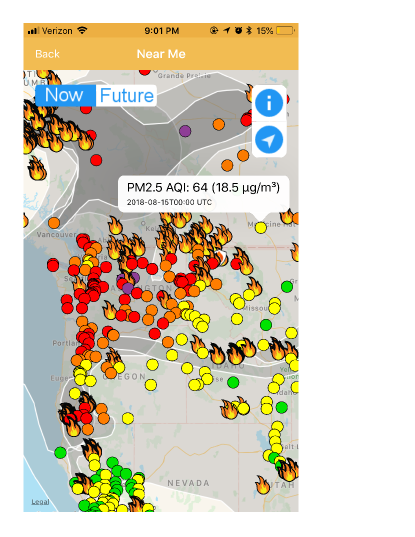
Figure 1: A screen shot of the Smoke Sense App alerting the user of local fires and air quality.

In this study, the outcome of interest is the number of user-reported adverse health symptoms during the 2019 smoke season, reported as weekly summaries. The weekly number of adverse events ranged from $1$ to $15$ with a mean (sd) of $5.1$ ($2.8$). The treatment is a binary indicator of whether the participant took strong protective behaviors – staying indoor with extra protective behaviors like using an air cleaner or a respirator mask. Other variables include the baseline information when registered in the app including age, gender, first 3-digits of the zip code, etc, and time-varying variables including self-reported smoke experience, days of visibility impacted, etc, which users are reminded of reporting every week. More details about the variables are provided in Supplementary Materials. In our analysis, we include $n=1076$ users who reported baseline and time-varying variables. Among these users, 205 reported more than once and the maximum number of reporting is $25$.

2.2 Wildfire smoke exposure

For each user-week, the exposure to smoke is determined based on HMS (http://satepsanone.nesdis.noaa.gov/pub/volcano/FIRE/HMS\_ARCHIVE/). The HMS data contains the spatial contours of satellite observed imagery of smoke together with the estimated density of fine particulate matter (${\rm PM}_{2.5}$) based on the air quality model. The smoke density is summarized by four levels: none, light (${\rm PM}_{2.5}$ range: $0-10$ $\mu g/m^{3}$, medium ($10.5-21.5$ $\mu g/m^{3}$), and dense ($\geq 22\mu g/m^{3}$), where each level is summarized by the midpoint of the corresponding range (0, 5, 16, and 27 $\mu g/m^{3}$, respectively). We map the highest daily exposure value to each zip code and aggregate the HMS data by taking the maximum value over the 3-digit zip code (zip3). We restrict our analysis to the time period from September 2018 to the end of 2019 and across zip3 where there were more than 10 smoke sense users. Figure 2 shows the map of the maximum weekly smoke density across zip3 geographic locations during the study period, where the west coast showed heavier wildland fire smoke occurrence.

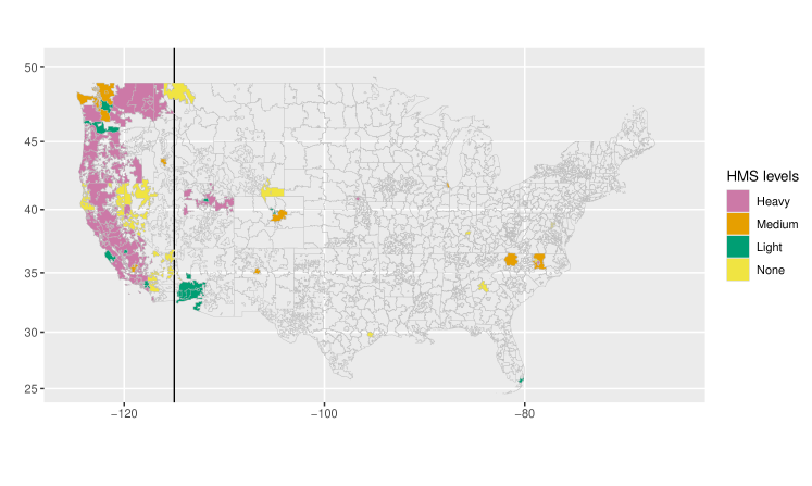
Figure 2: Maximum daily HMS smoke density level in each three-digit zip code over the study period. The smoke density has four levels: None, Light, Medium, and Heavy (corresponding to 0, 5, 16, and 27 $\mu g/m^{3}$, respectively). The vertical line is at longitude -115.

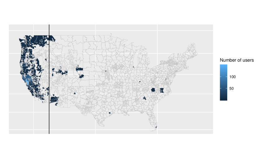
Figure 3: The number of users in each three-digit zip code over the study period. The vertical line is at longitude -115.

2.3 Notation

We follow the notation from the standard structural nested model literature (Robins, 1994). We assume $n$ subjects are monitored over time points $t_{0},\ldots,t_{K}$. For privacy concerns, the spatial location of the subjects are summarized by their 3-digit zip codes. To obtain the latitude and longitude of the spatial location, $\mathbf{s}=(s_{1},s_{2})$, we average the latitude and longitude coordinates over all the 5-digit zip codes which have the same 3-digit zip codes (the latitude and longitude coordinates corresponding to each 5-digit zip code are available at https://public.opendatasoft.com/explore/dataset/us-zip-code-latitude-and-longitude/export/). The subjects are assumed to be an independent sample, and for simplicity, we omit a subscript for subjects. Let $A_{k}$ be the binary treatment at $t_{k}$ ($A_{k}=1$ if the subject reported taking the strong protective behaviors, and $A_{k}=0$ if the subject did not take any behavior or took some mild protective behaviors). Let $X_{0}$ be a vector of baseline variables, including the subject’s demographic information (e.g., sex, age, race, education level), baseline health information (e.g., pre-existing conditions, physical activity level, time spent outdoors), and current beliefs about smoke and air pollution. Let $X_{k}\in\text{$\mathcal{X}_{k}$}$ be a vector of baseline covariates and time-varying variables at $t_{k}$ (e.g., the recent experience of smoke, feeling status, visibility). Let $Y_{k}$ be the outcome at $t_{k}$ (the total number of symptoms the subject had including e.g. anxiety, asthma attack, chest pain).

We use overbars to denote a variable’s history; e.g., $\bar{A}_{k}=\{A_{m}:m=0,\ldots,k\}$, and the complete history $\bar{A}_{K}$ abbreviates to $\bar{A}$. Let $Y_{k}^{(\bar{a})}$ be the outcome at $t_{k}$, possibly counterfactual, had the subject followed treatment regime $\bar{a}$ over the study period from $t_{0}$ to $t_{K}$. For simplicity, we use $Y_{k}^{(\bar{a}_{m})}$ $(m\leq k)$ to denote the potential outcome at $t_{k}$ had the subject followed treatment regime $\bar{a}_{m}$ until $t_{m}$ and no treatment onwards. We assume that the observed outcome $Y_{k}$ is equal to $Y_{k}^{(\bar{A})}$ for $k=0,\ldots,K$. Finally, $V=(\bar{A},\bar{X},\bar{Y})$ denotes the subject’s full records. Up to Section 5, we shall assume that all subjects’ full records are observed. We let $\mathbb{P}$ be the probability measure induced by $V$ and $\mathbb{P}_{n}$ be the empirical measure for $V_{1},...,V_{n}$; i.e., $\mathbb{P}_{n}f(V)=n^{-1}\sum_{i=1}^{n}f(V_{i})$ for any real-valued function $f(v)$.

3 Global structural nested mean models

The treatment effect is defined in terms of the expected value of potential outcomes under different treatment trajectories. Because both the treatment and outcome are longitudinal, and there may be a lag time between the treatment and its effect, we define the causal effect of the treatment at $t_{m}$ on the outcome at $t_{k}$ for $k\geq m$.

Definition 1 (Global SNMM)

For $0\leq m\leq k\leq K$, the treatment effect is characterized by

$$\text{E}\left\{Y_{k}^{(\bar{a}_{m-1},a_{m})}-Y_{k}^{(\bar{a}_{m-1},0)}\mid\bar{A}_{m-1}=\bar{a}_{m-1},\bar{X}_{m}=\bar{x}_{m}\right\}=\gamma_{m,k}(\psi^{*}),$$ (1)

where $\bar{a}_{-1}$ denotes a null set by convention, and $\gamma_{m,k}(\psi^{*})=\gamma_{m,k}(\bar{a}_{m},\bar{x}_{m};\psi^{*})$ is a known function of $(\bar{a}_{m},\bar{x}_{m})$ with a vector of unknown parameters $\psi^{*}\in\mathcal{R}^{p}$ with a fixed $p\geq 1$. That is, the causal effect is the expected difference in the response at $t_{k}$ between two counterfactual regimes with the same treatment before $t_{m}$, different treatment at $t_{m}$, and no treatments after $t_{m}$."

To help understand the model, consider the following example.

Example 1

Assume $\gamma_{m,k}(\psi^{*})=\psi^{*}a_{m}$, if $k=m$ and $0$ otherwise, where $\psi^{*}$ is a scalar.

This model entails that on average, the treatment $a_{m}$ at $t_{m}$ would increase the mean of the immediate outcome at $t_{m}$ by $\psi^{*}$ for subjects with $(\bar{A}_{m-1}=\bar{a}_{m-1},\bar{X}_{m}=\bar{x}_{m})$.

This framework can also include effect modifiers. For example, we can consider $\gamma_{m,k}(\psi^{*})=a_{m}(1,x_{m}^{\mathrm{\scriptscriptstyle T}})\psi^{*}$, where $x_{m}$ is a $(p-1)$-vector of the individual characteristics and $\psi^{*}=(\psi_{1}^{*},\ldots,\psi_{p}^{*})^{\mathrm{\scriptscriptstyle T}}$. Therefore, the class of SNMMs has important applications in precision medicine (Chakraborty and Moodie, 2013) for the discovery of optimal treatment regimes that are tailored to individuals’ characteristics and environments.

Parameter identification requires the typical sequential randomization assumption (Robins et al., 1992) that for $0\leq m\leq k\leq K$, $Y_{k}^{(\bar{a}_{m})}\mathbin{\mathchoice{\hbox to0.0pt{\hbox{$\displaystyle\perp$}\hss}\kern 3.46875pt{}\kern 3.46875pt\hbox{$\displaystyle\perp$}}{\hbox to0.0pt{\hbox{$\textstyle\perp$}\hss}\kern 3.46875pt{}\kern 3.46875pt\hbox{$\textstyle\perp$}}{\hbox to0.0pt{\hbox{$\scriptstyle\perp$}\hss}\kern 2.36812pt{}\kern 2.36812pt\hbox{$\scriptstyle\perp$}}{\hbox to0.0pt{\hbox{$\scriptscriptstyle\perp$}\hss}\kern 1.63437pt{}\kern 1.63437pt\hbox{$\scriptscriptstyle\perp$}}}A_{m}\mid\bar{L}_{m}$, where $\bar{L}_{m}$$=(\bar{A}_{m-1},\bar{X}_{m},\bar{Y}_{m-1})$. This assumption holds if $\bar{L}_{m}$ captures all confounders for the treatment at $t_{m}$ and ensuing outcomes. Define the propensity score as $e(\bar{L}_{m})=\mathrm{P}(A_{m}=1\mid\bar{L}_{m})$. Moreover, define $H_{k}^{(\bar{A}_{m-1})}(\psi^{*})=Y_{k}-\sum_{l=m}^{k}\gamma_{l,k}(\psi^{*})$ and $\mu_{m,k}(\bar{L}_{m})=\text{E}\{H_{k}^{(\bar{A}_{m-1})}(\psi)\mid\bar{L}_{m}\}$. Intuitively, $H_{k}^{(\bar{A}_{m-1})}(\psi^{*})$ removes the accumulated treatment effects from $t_{m}$ to $t_{k}$ from the observed outcome $Y_{k}$, so it mimics the potential outcome $Y_{k}^{(\bar{a}_{m-1})}$ had the subject followed $\bar{a}_{m-1}=\bar{A}_{m-1}$ but no treatment onwards. The sequential randomization assumption states that $Y_{k}^{(\bar{a}_{m-1})}$ and $A_{m}$ are independent given $\bar{L}_{m}$. Robins et al. (1992) showed that $H_{k}^{(\bar{A}_{m-1})}(\psi^{*})$ inherits this property in the sense that $\text{E}\{H_{k}^{(\bar{A}_{m-1})}(\psi)\mid A_{m},\bar{L}_{m}\}=\text{E}\{H_{k}^{(\bar{A}_{m-1})}(\psi)\mid\bar{L}_{m}\}$. As a result, with any measurable, bounded function $q_{k,m}:\bar{\mathcal{\mathcal{L}}}_{m}\rightarrow\mathcal{R}^{p}$,

$$G(V;\psi)=\sum_{m=1}^{K}\sum_{k=m}^{K}q_{k,m}(\bar{L}_{m})\left\{H_{k}^{(\bar{A}_{m-1})}(\psi)-\mu_{m,k}(\bar{L}_{m})\right\}\{A_{m}-e(\bar{L}_{m})\}$$ (2)

is unbiased at $\psi^{*}$. Then, under a regularity condition that $\text{E}\{\partial G(V;\psi)/\partial\psi\}$ is invertible, the solution to $\text{E}\{G(V;\psi)\}=0$ uniquely exists, and therefore $\psi^{*}$ is identifiable.

The estimating function $G(V;\psi)$ depends on $q_{k,m}(\bar{L}_{m})$. The choice of $q_{k,m}(\bar{L}_{m})$ does not affect the unbiasedness but estimation efficiency. We adopt an optimal form of $q_{k,m}(\bar{L}_{m})$ given in the Supplementary Material. With this choice, the solution to $\mathbb{P}_{n}G(V;\psi)=0$ has the smallest asymptotic variance compared to other choices (Robins, 1994).

4 Local structural nested means model

4.1 Spatially varying structural nested mean models

Global SNMMs in Section 3 allow time-varying treatment effects but not spatially varying treatment effects. We extend to a new class of models that allows modeling spatial treatment effect heterogeneity.

Definition 2 (Local SNMM)

For $0\leq m\leq k\leq K$, the treatment effect is characterized by

$$\text{E}\left\{Y_{k}^{(\bar{a}_{m-1},a_{m})}-Y_{k}^{(\bar{a}_{m-1},0)}\mid\bar{A}_{m-1}=\bar{a}_{m-1},\bar{X}_{m}=\bar{x}_{m}\right\}=\gamma_{m,k}\{\psi^{*}(\mathbf{s})\},$$ (3)

where $\bar{a}_{-1}$ denotes a null set by convention, and $\gamma_{m,k}\{\psi^{*}(\mathbf{s})\}=\gamma_{m,k}\{\bar{a}_{m},\bar{x}_{m};\psi^{*}(\mathbf{s})\}$ is a known function of $(\bar{a}_{m},\bar{x}_{m})$ with a vector of spatially varying parameters $\psi^{*}(\mathbf{s})\in\mathcal{R}^{p}$ with a fixed $p\geq 1$.

Consider the following example in parallel to Example 1.

Example 2

Assume $\gamma_{m,k}\{\psi^{*}(\mathbf{s})\}=\psi^{*}(\mathbf{s})a_{m},$ if $k=m$ and $0$ otherwise, where $\psi^{*}(\mathbf{s})=s_{1}+s_{2}$.

This model entails that on average, the treatment would increase the mean of the outcome for subjects at time $t_{m}$ and location $\mathbf{s}$ had the subject received the treatment at $t_{m}$ by $\psi^{*}(\mathbf{s})a_{m}$, and the treatment effect surface over the study region is a tilted plane.

Similar with the global SNMM, we define $H_{k}^{(\bar{A}_{m-1})}\{\psi^{*}(\mathbf{s})\}=Y_{k}-\sum_{l=m}^{k}\gamma_{l,k}\{\psi^{*}(\mathbf{s})\}$. Following Robins et al. (1992), $H_{k}^{(\bar{A}_{m-1})}\{\psi^{*}(\mathbf{s})\}$ inherits this property in the sense that

$$G\{V;\psi(\mathbf{s})\}=\sum_{m=1}^{K}\sum_{k=m}^{K}q_{k,m}(\bar{L}_{m})\left[H_{k}^{(\bar{A}_{m-1})}\{\psi(\mathbf{s})\}-\mu_{m,k}(\bar{L}_{m})\right]\{A_{m}-e(\bar{L}_{m})\}$$ (4)

is unbiased at $\psi^{*}(s)$ with any measurable, bounded function $q_{k,m}:\bar{\mathcal{\mathcal{L}}}_{m}\rightarrow\mathcal{R}^{p}$.

4.2 Geographically weighted local polynomial estimation

There are an infinite number of parameters because $\psi^{*}(\mathbf{s})$ varies over $\mathbf{s}$. Estimation of $\psi^{*}(\mathbf{s})$ at a given $\mathbf{s}$ may become unstable with only a few observations at $\mathbf{s}$, or even infeasible at locations without any observations. To make estimation feasible, one can make some global structural assumptions about $\psi^{*}(\mathbf{s})$ with a fixed number of unknown parameters. However, this approach is sensitive to model misspecification. To overcome this difficulty, we combine the ideas of local polynomial approximation and geographically weighted regression. That is, we leave the global structure of $\psi^{*}(\mathbf{s})$ unspecified but approximate $\psi^{*}(\mathbf{s})$ locally by polynomials of $\mathbf{s}$. Then, we use geographical weighting to estimate the local parameters by pooling nearby observations whose contributions diminish with geographical distance.

To be specific, we consider estimating $\psi^{*}(\mathbf{s}^{*})$ at a given $\mathbf{s}^{*}.$ We approximate $\psi^{*}(\mathbf{s})=\{\psi_{1}^{*}(\mathbf{s}),\ldots,\psi_{p}^{*}(\mathbf{s})\}^{\mathrm{\scriptscriptstyle T}}$ in the neighborhood of $\mathbf{s}^{*}$ by the first-order local polynomial,

$$\widetilde{\psi}_{\mathrm{lp}}(\mathbf{s};\phi)=\left(\begin{array}[]{c}\phi_{1}^{\mathrm{\scriptscriptstyle T}}d(\mathbf{s}^{*}-\mathbf{s})\\ \vdots\\ \phi_{p}^{\mathrm{\scriptscriptstyle T}}d(\mathbf{s}^{*}-\mathbf{s})\end{array}\right)_{p\times 1},\ \phi_{j}=\left(\begin{array}[]{c}\phi_{j,0}\\ \phi_{j,1}\\ \phi_{j,2}\end{array}\right)_{3\times 1},\ d(\mathbf{s}^{*}-\mathbf{s})=\left(\begin{array}[]{c}1\\ s_{1}^{*}-s_{1}\\ s_{2}^{*}-s_{2}\end{array}\right)_{3\times 1},$$

and $\phi=(\phi_{1,0},\ldots,\phi_{p,0},\phi_{1,1},\ldots,\phi_{p,1},\phi_{1,2},\ldots,\phi_{p,2})^{\mathrm{\scriptscriptstyle T}}$ is the vector of unknown coefficients. Although we use the first-order local polynomial approximation, extensions to higher-order approximations are straightforward with heavier notation. As established in Section 2, $\psi^{*}(\mathbf{s}^{*})$ is identified based on the estimating function (2), so we adopt the local estimating equation approach (Carroll et al., 1998) with geographical weighting. We propose a geographically weighted estimator $\widehat{\phi}_{\tau}(\mathbf{s}^{*})$ by solving

$$\mathbb{P}_{n}\left[\omega_{\tau}(||\mathbf{s}^{*}-\mathbf{s}||)d(\mathbf{s}^{*}-\mathbf{s})\otimes G\{V;\widetilde{\psi}_{\mathrm{lp}}(\mathbf{s};\phi)\}\right]=0,$$ (5)

for $\phi$, where $M_{1}\otimes M_{2}$ denotes the Kronecker product of $M_{1}$ and $M_{2}$, and $\omega_{\tau}(\cdot)$ is a spatial kernel function with a scale parameter $\tau$. The first $p$-vector $\widehat{\phi}_{\tau,0}(\mathbf{s}^{*})$ in $\widehat{\phi}_{\tau}(\mathbf{s}^{*})$ estimates $\psi^{*}(\mathbf{s}^{*})$. The estimating equation (5) assigns more weight to observations nearby than those far from the location $\mathbf{s}^{*}.$ The commonly-used weight function is $\omega_{\tau}(||\mathbf{s}^{*}-\mathbf{s}||)=\tau^{-1}K\{||\mathbf{s}^{*}-\mathbf{s}||/\tau\}$, where $K(\cdot)$ is the Gaussian kernel density function. The scale parameter $\tau$ is the bandwidth determining the scale of spatial treatment effect heterogeneity; $\psi^{*}(\mathbf{s})$ is smooth over $\mathbf{s}$ when $\tau$ is large, and vice versa.

We illustrate the geographically weighted estimator of $\psi^{*}(\mathbf{s}^{*})$ with a simple example, which allows an analytical form.

Example 3

For the spatially varying structural nested mean model in Example 2, the geographically weighted estimator of $\psi^{*}(\mathbf{s}^{*})$ is the first component $\widehat{\phi}_{\tau,0}(\mathbf{s}^{*})$ of

$$\widehat{\phi}_{\tau}(\mathbf{s}^{*}) = \Gamma^{-1}\mathbb{P}_{n}\left[\omega_{\tau}(||\mathbf{s}^{*}-\mathbf{s}||)d(\mathbf{s}^{*}-\mathbf{s})\sum_{m=1}^{K}q_{m,m}(\bar{L}_{m})\left\{Y_{m}-\widehat{\mu}_{m,m}(\bar{L}_{m})\right\}\{A_{m}-e(\bar{L}_{m})\}\right],$$

$$\Gamma = \mathbb{P}_{n}\left[\omega_{\tau}(||\mathbf{s}^{*}-\mathbf{s}||)d(\mathbf{s}^{*}-\mathbf{s})^{\otimes 2}\vphantom{\sum_{1}^{K}}\sum_{m=1}^{K}q_{m,m}(\bar{L}_{m})A_{m}\{A_{m}-e(\bar{L}_{m})\}\right],$$

where $q_{m,m}(\bar{X}_{m})=\{1-e(\bar{L}_{m})\}\mathrm{var}[H_{m}^{(\bar{A}_{m-1})}\{\psi(\mathbf{s})\}\mid\bar{L}_{m}]^{-1}$ , and $M^{\otimes 2}$ denotes $MM^{\mathrm{\scriptscriptstyle T}}.$

The solution $\widehat{\phi}_{\tau}(\mathbf{s}^{*})$ to (5) is not feasible to calculate because it depends on the unknown distribution through $\mu_{m,k}(\bar{L}_{m})$ and $e(\bar{L}_{m})$. Therefore, we require positing models for and estimating the two nuisance functions.

The proposed estimation procedure proceeds as follows.

Step  3.1.

Fit a propensity score model, denoted by $\widehat{e}(\bar{L}_{m})$.

Step  3.2.

For each observed location $\mathbf{s}^{*}$, obtain a preliminary estimator $\widehat{\phi}_{\tau}^{[0]}(\mathbf{s}^{*})$ by solving

$$\mathbb{P}_{n}\left[\omega_{\tau}(||\mathbf{s}^{*}-\mathbf{s}||)d(\mathbf{s}^{*}-\mathbf{s})\otimes G^{[0]}\{V;\widetilde{\psi}_{\mathrm{lp}}(\mathbf{s};\phi)\}\right]=0,$$ (6)

for $\phi$, where $G^{[0]}\{V;\psi(\mathbf{s})\}=\sum_{m=1}^{K}\sum_{k=m}^{K}H_{k}^{(\bar{A}_{m-1})}\{\psi(\mathbf{s})\}\{A_{m}-\widehat{e}(\bar{L}_{m})\}$. Then, $\widehat{\phi}_{\tau,0}^{[0]}(\mathbf{s}^{*})$, the first $p$-vector in $\widehat{\phi}_{\tau}^{[0]}(\mathbf{s}^{*})$, is a preliminary estimator of $\psi^{*}(\mathbf{s}^{*})$. Using the pseudo outcome $H_{k}^{(\bar{A}_{m-1})}\left\{\widehat{\phi}_{\tau,0}^{[0]}(\mathbf{s}^{*})\right\}$ and $\bar{L}_{m}$, fit an outcome mean model, denoted by $\widehat{\mu}_{m,k}(\bar{L}_{m})$.

Step  3.3.

Obtain $\widehat{\phi}_{\tau}(\mathbf{s}^{*})$ by solving (5) with $e(\bar{L}_{m})$ and $\mu_{m,k}(\bar{L}_{m})$ replaced by their estimates in Steps 3.1 and 3.2. The proposed estimator of $\psi^{*}(\mathbf{s}^{*})$ is the first $p$-vector $\widehat{\phi}_{\tau,0}(\mathbf{s}^{*})$ of $\widehat{\phi}_{\tau}(\mathbf{s}^{*})$.

Remark 1

It is worth discussing an alternative way to approximate $\mu_{m,k}(\bar{L}_{m})$ by noticing that $\mu_{m,k}(\bar{L}_{m})=\text{E}\{Y_{k}^{(\bar{A}_{m-1})}\mid\bar{L}_{m}\}$. It amounts to identifying subjects who followed a treatment regime $(\bar{A}_{m-1},\bar{0})$ and fitting the outcome mean model based on $Y_{k}$ and $\bar{L}_{m}$ among these subjects.

4.3 Asymptotic properties

We show that the proposed estimator has an appealing double robustness property in the sense that the consistency property requires that one of the nuisance function models is correctly specified, not necessarily both. This property adds protection against possible misspecification of the nuisance models. Below, we establish the asymptotic properties of $\widehat{\phi}_{\tau,0}(\mathbf{s}^{*})$, including robustness, asymptotic bias and variance. Assume the observed locations are continuously distributed over a compact study region. Let $f_{\mathbf{s}}(\mathbf{s})$ be the marginal density of the observed locations $\mathbf{s}$, which is bounded away from zero. Also, assume that $\psi(\mathbf{s})$ is twice differentiable with bounded derivatives. The kernel function $K(\cdot)$ is bounded and symmetric with $\int\mathbf{s}^{2}K(\mathbf{s})\mathrm{d}\mathbf{s}=\int\mathbf{s}^{2}K(\mathbf{s})\mathrm{d}\mathbf{s}=1$, and the bandwidth satisfies $\tau\rightarrow 0$ and $n\tau^{2}\rightarrow\infty$ as $n\rightarrow\infty$.

Theorem 1

Suppose Assumption 1, the sequential randomization assumption and the regularity conditions presented in the Supplementary Material hold. Let $\widehat{\phi}_{\tau}(\mathbf{s}^{*})$ be the solution to (5) with $\mu_{m,k}(\bar{L}_{m})$ and $e(\bar{L}_{m})$ replaced by their estimates $\widehat{\mu}_{m,k}(\bar{L}_{m})$ and $\widehat{e}(\bar{L}_{m})$. Let $\widehat{\phi}_{\tau,0}(\mathbf{s}^{*})=e_{1}^{\mathrm{\scriptscriptstyle T}}\widehat{\phi}_{\tau}(\mathbf{s}^{*}),$ where $e_{1}=(I_{p\times p},0_{p\times p},0_{p\times p})^{\mathrm{\scriptscriptstyle T}}$. If either $\mu_{m,k}(\bar{L}_{m})$ or $e(\bar{L}_{m})$ is correctly specified, $\widehat{\phi}_{\tau,0}(\mathbf{s}^{*})$ is consistent for $\psi^{*}(\mathbf{s}^{*})$, and

$$\left\{n\tau^{2}f_{\mathbf{s}}(\mathbf{s}^{*})\right\}^{-1/2}\left\{\widehat{\phi}_{\tau,0}(\mathbf{s}^{*})-\psi^{*}(\mathbf{s}^{*})-\tau^{2}\mathcal{G}_{b}(\mathbf{s}^{*})\right\}\rightarrow\mathcal{N}\{0_{p\times 1},\mathcal{G}_{v}(\mathbf{s}^{*})\},$$

where $\mathcal{G}_{b}\{\mathbf{s}^{*},K,\psi(\mathbf{s}^{*})\}$ and $\mathcal{G}_{v}\{\mathbf{s}^{*},K,\psi(\mathbf{s}^{*})\}$ do not depend on $\tau$.

The proof and the expressions of $\mathcal{G}_{b}\{\mathbf{s}^{*},K,\psi(\mathbf{s}^{*})\}$ and $\mathcal{G}_{v}\{\mathbf{s}^{*},K,\psi(\mathbf{s}^{*})\}$ are presented in the Supplementary Material.

4.4 Bandwidth selection using a balancing criterion

We use the K-fold cross-validation to select the bandwidth $\tau$. An important question arises about the loss function. We propose a new objective function using a balancing criterion. The key insight is that with a good choice of $\tau,$ the mimicking potential outcome $H_{k}^{(\bar{A}_{m-1})}\{\widehat{\phi}_{\tau,0}(\mathbf{s}^{*})\}$ is approximately uncorrelated to $A_{m}$ given $\bar{L}_{m}$; therefore, the distribution of $H_{k}^{(\bar{A}_{m-1})}\{\widehat{\phi}_{\tau,0}(\mathbf{s}^{*})\}$ is balanced between $A_{m}=1$ and $A_{m}=0$ among the group with the same $\bar{L}_{m}$. If $\bar{L}_{m}$ contains continuous variables, the balance measure is difficult to formulate because it involves forming subgroups by collapsing observations with similar values of $\bar{L}_{m}$. To avoid this issue, inspired by the estimating functions, we formulate the loss function as

$$G_{\mathrm{loss}}\{V;\psi(\mathbf{s}^{*})\}=\left|\mathbb{P}_{n}\omega_{\tau}(||\mathbf{s}^{*}-\mathbf{s}||)\vphantom{\sum_{k}^{K}}\right.\\ \left.\times\sum_{m=1}^{K}\sum_{k=m}^{K}\left[H_{k}^{(\bar{A}_{m-1})}\{\widehat{\phi}_{\tau,0}(\mathbf{s}^{*})\}\right.\left.\vphantom{H_{k}^{(\bar{A})}}-\widehat{\mu}_{m,k}(\bar{L}_{m})\right]\{A_{m}-\widehat{e}(\bar{L}_{m})\}\right|.$$ (7)

If $\tau$ is too small, $\widehat{\phi}_{\tau,0}(\mathbf{s}^{*})$ has a large variance and also $\omega_{\tau}(||\mathbf{s}^{*}-\mathbf{s}||)$ is only nontrivial for few locations in the $\tau$-neighborhood of $\mathbf{s}^{*}$, which leads to a large value of $G_{\mathrm{loss}}\{V;\psi(\mathbf{s}^{*})\}$; while if $\tau$ is too large, $\widehat{\phi}_{\tau,0}(\mathbf{s}^{*})$ has a large bias, which translates to a large loss too. Therefore, a good choice of $\tau$ balances the trade-off between variance and bias.

4.5 Bias correction

Theorem 1 provides the asymptotic bias formula, which however involves derivatives of $\psi^{*}(\mathbf{s}^{*})$ and is difficult to approximate. Following Ruppert (1997), we extend the empirical bias bandwidth selection method to the geographically weighted framework. For a fixed location $\mathbf{s}^{*},$ we calculate $\widehat{\phi}_{\tau,0}(\mathbf{s}^{*})$ at a series of $\tau$ over a pre-specified range $\mathcal{T}=\{\tau_{1},\ldots,\tau_{L}\},$ where $L$ is at least $3$. Based on Theorem 1, the bias function of $\widehat{\phi}_{\tau,0}(\mathbf{s}^{*})$, with respect to $\tau,$ is of order $\tau^{2}$. This motivates a bias function of a form $b(\tau;\nu)=\nu_{1}\tau^{2}+\cdots+\nu_{1+q}\tau^{1+q}$, where $q$ is an integer greater than $2$ and $\nu=(v_{1},\ldots,\nu_{1+q})^{\mathrm{\scriptscriptstyle T}}$ is a vector of unknown coefficients. Based on the pseudo data $\{\tau,\widehat{\phi}_{\tau,0}(\mathbf{s}^{*}):\tau\in\mathcal{T}\}$, fit a function $\text{E}\{\widehat{\phi}_{\tau,0}(\mathbf{s}^{*})\}=\nu_{0}+b(\tau;\nu)$ to obtain $\widehat{\nu}$. Then, we estimate the bias of $\widehat{\phi}_{\tau,0}(\mathbf{s}^{*})$ by $b(\tau;\widehat{\nu}).$ The debiasing estimator is $\widehat{\phi}_{\tau,0}^{\mathrm{bc}}(\mathbf{s}^{*})=\widehat{\phi}_{\tau,0}(\mathbf{s}^{*})-b(\tau;\widehat{\nu})$.

4.6 Wild bootstrap inference

For variance estimation, Carroll et al. (1998) proposed using the sandwich formula in line with the Z-estimation literature. The sandwich formula is justified based on asymptotics. To improve the finite-sample performance, Galindo et al. (2001) proposed a bootstrap inference procedure for local estimating equations. However, this procedure involves constructing complicated residuals and a heuristic modification factor. Thus, we suggest an easy-to-implement wild bootstrap method for variance estimation of $\widehat{\phi}_{\tau,0}^{\mathrm{bc}}(\mathbf{s}^{*})$.

For each bootstrap replicate, we generate exchangeable random weights $\xi_{i}$ ($i=1,\ldots,n$ ) independent and identically distributed from a distribution that has mean one, variance one and is independent of the data; e.g., Exp$(1)$. Repeat the cross-validation for choosing $\tau$, calculation of $\widehat{\phi}_{\tau,0}(\mathbf{s}^{*})$, and bias-correction steps but all steps are carried out using weighted analysis with $\xi_{i}$ for subject $i$. Importantly, we do not need to re-estimate the nuisance functions for each bootstrap replication, because they converge faster than the geographically weighted estimator. This feature can largely reduce the computational burden in practice. The variance estimate $\widehat{V}(\mathbf{s}^{*})$ of $\widehat{\phi}_{\tau,0}^{\mathrm{bc}}(\mathbf{s}^{*})$ is the empirical variance of a large number of bootstrap replicates. With the variance estimate, we can construct the Wald-type confidence interval as $\widehat{\phi}_{\tau,0}^{\mathrm{bc}}(\mathbf{s}^{*})\pm z_{1-\alpha/2}\left\{\widehat{V}(\mathbf{s}^{*})\right\}^{1/2}$.

5 Extension to the settings with non-responses

In large longitudinal observational studies, non-responses are ubiquitous. To accommodate non-responses, let $\bar{R}=(R_{0},\ldots,R_{K})$ be the vector of response indicators; i.e., $R_{m}=1$ if the subject responded at $t_{m}$ and $0$ otherwise. With a slight abuse of notation, let $V=(\bar{A},\bar{X},\bar{Y},\bar{R})$ be the full data. Let $\pi_{m}(V)=P(R_{m}=1\mid V)$ be the response probability at $t_{m}$. If the response probabilities are known, an inverse probability weighted estimating function

$$G_{\mathrm{ipw}}\{V;\psi(\mathbf{s})\}=\sum_{m=1}^{K}\left\{\sum_{k=m}^{K}\omega_{m:k}(\bar{R})q_{k,m}(\bar{L}_{m})\left[H_{k}^{(\bar{A}_{m-1})}\{\psi(\mathbf{s})\}-\mu_{m,k}(\bar{L}_{m})\right]\right\}\\ \times\{A_{m}-e(\bar{L}_{m})\},$$ (8)

is unbiased at $\psi^{*}(\mathbf{s})$, where $\omega_{m:k}(\bar{R})=\prod_{l=m}^{k}\{R_{l}{\pi_{l}(V)}^{-1}\}$ is the inverse probability weights of responding from $t_{m}$ to $t_{k}$. The geographically weighted local polynomial framework applies by using (8) for estimating $\psi^{*}(\mathbf{s}^{*})$.

In practice, $\pi_{m}(V)$ is unknown. We require further assumptions for identification and estimation of $\pi_{m}(V)$. The most common approach makes a missingness at random assumption (Rubin, 1976) that $\pi_{m}(V)$ depends only on the observed data but not the missing values. In smartphone applications with subject-initiated reporting, whether subjects reported or not is likely to depend on their current status. Then, the response mechanism depends on the possibly missing values themselves, leading to an informative non-response mechanism. In these settings, one can utilize a non-response instrument to help identification and estimation of $\pi_{m}(V)$ (Wang et al., 2014, Li et al., 2020). For illustration, we assume a simple informative response mechanism that $\pi_{m}(V)=\pi(V_{m})$, where $V_{m}=(A_{m},X_{m},Y_{m},\bar{R}_{m-1})$; i.e., $\pi_{m}(V)$ depends only on the current (possibly missing) status $(A_{m},X_{m},Y_{m})$ and the number of historical responses. Extension to more complicated mechanisms is possible at the expense of heavier notation. We then posit a parametric response model, denoted by $\pi_{m}(V_{m};\eta^{*})$ with an unknown parameter $\eta^{*}\in\mathcal{R}^{d}$. For informative non-responses, the parameter $\eta^{*}$ is not identifiable even with a parametric model (Wang et al., 2014). We assume that there exists an auxiliary variable $Z_{m}$ called a non-response instrument that can be excluded from the non-response probability, but are associated with the current status even when other covariates are conditioned (see Condition C1 in Theorem 1 of Wang et al., 2014 for the formal definition). Existence of such non-response instruments depends on the study context and available data. For example, in the Smoke Sense initiative, a valid non-response instrument is the smoke plume data HMS measured at monitors, which is related to the subject’s variables but is unrelated to whether the subject reporting or not after controlling for subject’s own perceptions about risk.

With a valid instrument, $\eta^{*}$ is identifiable. Following Robins and Rotnitzky (1997), $\widehat{\eta}$ can be obtained by solving

$$\mathbb{P}_{n}\sum_{m=0}^{K}\left\{\frac{R_{m}}{\pi_{m}(V_{m};\eta)}-1\right\}h(Z_{m},\bar{R}_{m-1})=0,$$ (9)

where $h(Z_{m},\bar{R}_{m-1})\in\mathbb{\mathcal{R}}^{d}$ is a function of $(Z_{m},\bar{R}_{m-1})$. An additional complication involves estimating the nuisance functions $\mu_{m,k}(\bar{L}_{m})$ and $e(\bar{L}_{m})$ in the presence of non-response, which now requires weighting similar to that in (8). We present the technical details in the Supplementary Material.

6 Simulation

We evaluate the finite-sample performance of the proposed estimator on simulated datasets to evaluate the double robustness property. We first consider the simpler case without non-responses in Section 6.1 and then consider the case with non-responses in Section 6.2 to mimic the Smoke Sense data.

6.1 Complete data without non-responses

In this section, we simulate $500$ datasets without non-response. In each dataset, we generate $n=400$ locations uniformly over a unit square. For each location, the subject’s covariate process over $K=25$ weeks, $\bar{X}$, follows a Gaussian process with mean $0$, variance $0.5$ and a first-order autocorrelation structure with lag-1 correlation $0.5$. We generate the potential outcome process as $Y_{k}^{(\bar{0})}=X_{k}+\epsilon_{k}$, for $k=1,\ldots,K$, where $\bar{\epsilon}$ follows a Gaussian process with mean $0$, variance $0.25$, and a first-order autocorrelation structure with lag-1 correlation $0.25$. We generate the treatment process as $\bar{A}$, where $A_{k}\sim$ Binomial{$e(\bar{L}_{k})$} with logit$\{e(\bar{L}_{k})\}=-1+0.5X_{k}+0.25$cum$(\bar{A}_{k-1})$ and cum$(\bar{A}_{k-1})=\sum_{m=0}^{k-1}A_{m}$. The observed outcome process is $Y_{k}=Y_{k}^{(\bar{0})}+\sum_{m=0}^{k-1}\gamma_{m,k}\{\psi^{*}(\mathbf{s})\}$, where $\gamma_{m,k}\{\psi^{*}(\mathbf{s})\}=\psi^{*}(\mathbf{s})A_{m},$ if $k=m+1$ and zero otherwise. We consider three treatment effect specifications for location $\mathbf{s}=(s_{1},s_{2})$:

1. $\psi^{*}(\mathbf{s})=s_{1}+s_{2}$;

2. $\psi^{*}(\mathbf{s})=\exp(s_{1}+s_{2})$;

3. $\psi^{*}(\mathbf{s})=\sin\{2(s_{1}+2s_{2}-1)\}$.

We then consider estimating $\psi^{*}(\mathbf{s}^{*})$ at four locations with $\mathbf{s}^{*}=(s_{1}^{*},s_{2}^{*})$ and $s_{j}^{*}\in\{0.25,0.75\}$ ($j=1,2$).

To investigate the double robustness in Theorem 1, we consider two models for $\mu_{m,k}(\bar{L}_{m})$: (a) a correctly specified linear regression model and (b) a misspecified model by setting $\widehat{\mu}_{m,k}(\bar{L}_{m})=0$. We also consider two models for $e(\bar{L}_{m})$: (a) a correctly specified logistic regression model with predictors $X_{m}$ and cum$(\bar{A}_{m-1})$ and (b) a misspecified logistic regression model with predictors $X_{m}^{2}$ and cum$(\bar{A}_{m-1})^{2}$. For all estimators, we consider a grid of geometrically spaced values for $\tau$ from $\{\exp(0.005),\exp(0.05)\}$ and use 5-fold cross validation in Section 4.4 to choose $\tau.$ We use the wild bootstrap procedure for variance estimation with the bootstrap size $50$.

Table 1 reports the simulation results for Scenarios (S1)–(S3), respectively. When either the model for the propensity score or the model for the outcome mean is correctly specified, the proposed estimator has small bias for all treatment effects at all locations across three scenarios. These results confirm the double robustness in Theorem 1. Moreover, under these cases, the wild bootstrap provides variance estimates that are close to the true variances and good coverage rates that are close to the nominal level.

Table 1: Simulation results for complete data. The Monte Carlo average ($\times 10^{2},$ Est) and variance ($\times 10^{3}$, Var) of the estimators, variance estimators ($\times 10^{3}$, Ve), and coverage rate ($\%$, Cr) of $95\%$ confidence intervals. The three scenarios (S1)-(S3) are different values of the true spatially varying effect, and the results are reported separately for four fixed locations ($\mathbf{s}_{1}^{*}$-$\mathbf{s}_{4}^{*}$). The methods vary by whether they have the correct model for the outcome mean $\mu_{m,k}(\bar{L}_{m})$ and the propensity score $e({\bar{L}}_{m})$.

		Scenario (S1)					Scenario (S2)					Scenario (S3)
		$\mathbf{s}_{1}^{*}$	$\mathbf{s}_{2}^{*}$	$\mathbf{s}_{3}^{*}$	$\mathbf{s}_{4}^{*}$		$\mathbf{s}_{1}^{*}$	$\mathbf{s}_{2}^{*}$	$\mathbf{s}_{3}^{*}$	$\mathbf{s}_{4}^{*}$		$\mathbf{s}_{1}^{*}$	$\mathbf{s}_{2}^{*}$	$\mathbf{s}_{3}^{*}$	$\mathbf{s}_{4}$
	True	50.0	100.0	100.0	150.0		164.9	271.8	271.8	448.2		-47.9	47.9	99.7	59.80
Propensity score model $(\checked)$
	Est	50.1	99.2	99.6	149.7		165.8	270.0	270.4	449.6		-47.4	49.0	100.8	57.2
Mean	Var	18.5	14.2	17.5	16.5		18.9	14.6	17.7	18.0		17.0	13.7	16.9	18.1
model $(\checked)$	Ve	16.7	16.7	16.8	17.2		16.9	16.5	16.8	18.5		17.1	17.0	18.0	19.4
	Cr	93.0	96.0	94.6	95.0		93.2	96.2	94.6	94.8		93.4	95.8	95.0	93.8
	Est	51.4	99.9	99.8	152.0		167.4	270.7	270.6	451.8		-45.8	49.9	100.6	59.3
Mean	Var	37.5	31.8	39.2	34.6		36.3	33.8	39.0	35.2		36.9	33.0	37.5	37.6
model $(\times)$	Ve	38.0	36.2	36.7	35.5		37.9	36.0	37.0	36.3		37.9	36.4	37.4	38.1
	Cr	93.6	96.6	94.0	95.0		93.6	96.2	95.0	94.4		94.2	95.4	94.8	95.40
Propensity score model $(\times)$
	Est	50.1	99.3	99.5	150.0		166.0	269.9	270.3	449.9		-47.1	49.0	100.3	57.4
Mean	Var	19.6	15.8	17.3	18.6		19.6	16.3	17.2	19.7		20.8	16.7	16.9	21.10
model $(\checked)$	Ve	18.6	17.8	18.8	18.8		18.8	17.8	19.0	20.1		18.9	18.1	19.7	20.80
	Cr	93.4	96.0	94.8	95.6		93.6	95.8	94.6	93.8		92.4	95.2	95.6	94.8
	Est	97.7	147.0	146.6	198.4		213.5	317.9	317.4	498.1		0.1	96.9	147.7	106.0
Mean	Var	37.3	34.8	49.6	32.1		38.0	36.3	48.9	33.6		33.9	35.7	48.7	36.0
model $(\times)$	Ve	37.4	38.6	37.0	37.0		37.6	36.3	36.8	37.9		38.0	38.9	38.3	40.3
	Cr	22.4	23.0	22.4	23.8		22.0	25.0	23.6	24.6		22.6	19.4	22.4	29.0

$\checked$ (is correctly specified), $\times$ (is misspecified)

6.2 Informative non-responses

In this section, we generate data with informative non-responses. The data generating processes are the same as in Section 6.1, except that we further generate the vector of response indicators $\bar{R},$ where $R_{k}\sim$ Binomial{$\pi_{k}(Y_{k},\bar{R}_{k-1})$} with logit$\{\pi_{k}(Y_{k},\bar{R}_{k-1})\}=-1+0.5Y_{k}+0.25$cum$(\bar{R}_{k-1})$. If $R_{k}=1$, $(A_{k},X_{k},Y_{k})$ is observed, otherwise only $X_{k}$ is observed. Thus, $X_{k}$ is a non-response instrument. We compare the following estimators.

GWLPc1:

the geographically weighted local polynomial estimator with the non-response weights setting to a constant $1$, which corresponds to the proposed estimator with a misspecified model for the non-response probability;

GWLPipw:

the proposed geographically weighted local polynomial estimator with inverse probability of non-response weighting adjustment.

For both estimators, we consider correctly specified models for the outcome mean and propensity score. We use the same cross-validation and wild bootstrap procedures as in Section 6.

Table 2 reports the simulation results with informative non-responses for Scenarios (S1)–(S3). The GWLPc1 estimator without the inverse probability of non-response weighting adjustment is biased, and its coverage rate is off the nominal level, suggesting that informative missingness would lead to biased conclusions. The GWLPipw estimator with proper weighting adjustment has small bias for all locations across all scenarios.

Table 2: Simulation results for data with informative non-responses. The Monte Carlo average ($\times 10^{2},$ Est) and variance ($\times 10^{3}$, Var) of the estimators, variance estimators ($\times 10^{3}$, Ve), and coverage rate ($\%$, Cr) of $95\%$ confidence intervals. The three scenarios (S1)-(S3) are different values of the true spatially varying effect, and the results are reported separately for four fixed locations ($\mathbf{s}_{1}^{*}$-$\mathbf{s}_{4}^{*}$). The methods vary by whether they have the correct (GWLPipw) or incorrect (GWLPc1) model for the missing data mechanism ($\pi_{m})$.

		Scenario (S1)					Scenario (S2)					Scenario (S3)
		$\mathbf{s}_{1}^{*}$	$\mathbf{s}_{2}^{*}$	$\mathbf{s}_{3}^{*}$	$\mathbf{s}_{4}^{*}$		$\mathbf{s}_{1}^{*}$	$\mathbf{s}_{2}^{*}$	$\mathbf{s}_{3}^{*}$	$\mathbf{s}_{4}^{*}$		$\mathbf{s}_{1}^{*}$	$\mathbf{s}_{2}^{*}$	$\mathbf{s}_{3}^{*}$	$\mathbf{s}_{4}^{*}$
	True	50.00	100.00	100.0	150.0		164.9	271.8	271.8	448.2		-47.9	47.9	99.7	59.8
	Est	50.6	102.2	101.0	149.3		163.8	271.0	270.4	450.0		-42.9	52.0	101.3	59.0
Missing data	Var	101.8	102.8	80.5	79.8		63.7	43.2	40.4	44.0		148.3	112.4	71.2	91.1
model $(\checked)$	Ve	135.4	101.6	114.5	70.7		60.5	46.1	46.0	40.5		210.3	123.0	115.5	100.3
	Cr	92.2	94.4	94.8	91.6		93.4	95.4	94.6	92.8		92.2	93.6	94.2	91.8
	Est	42.8	86.4	86.6	132.1		158.2	260.2	260.2	434.0		-45.4	41.1	87.1	48.1
Missing data	Var	45.4	32.4	25.0	25.8		44.5	27.9	33.8	29.3		57.8	26.6	24.4	31.9
model $(\times)$	Ve	38.2	30.1	32.6	24.2		57.6	29.6	29.7	26.2		70.8	31.5	28.3	44.4
	Cr	93.4	83.8	82.4	74.6		91.4	88.4	86.8	83.0		93.6	93.0	78.0	85.6

$\checked$ (is correctly specified), $\times$ (is misspecified)

7 Smoke Sense data application

We now apply the new methodology to the Smoke Sense data to estimate heterogeneous effects of protective measures to mitigate the impact of wildland fire smoke. We follow the basic setup in Section 2, where the data are recorded monthly ( $t_{k}=k$ is the $k$th month after registration).

To model the treatment effect, a complication raises because taking protective behaviors might not have immediate effects on health outcomes and also the effect on the future outcomes eventually reduces to zero for large time lags. Taking these features into account, we consider the treatment effect model of a squared exponential function of the time lag $(t_{k}-t_{m})$ as

$$\gamma_{m,k}(\psi^{*})=\psi\exp\left\{-\frac{(t_{k}-t_{m}-\mu)^{2}}{2\sigma^{2}}\right\}a_{m},$$ (10)

where $\psi^{*}=(\psi,\mu,\sigma^{2})$ is the vector of parameters. Model (10) captures the key features of the treatment effect curve (see Figure 4): the effect of treatment $a_{m}$ on future health outcomes increases smoothly over time, reaches to a peak after $\mu$ units of time, and decreases to zero as time further increases. Moreover, a negative sign of $\psi$ indicates that the treatment is beneficial in reducing the number of adverse health outcomes, a larger magnitude of $\psi$ means a larger maximum treatment effect, vice versa, and $\sigma$ determines the duration of the effect across time lags. We consider fitting a global model (10) in Section 7.1 and a local model with spatially varying $\psi^{*}(\mathbf{s})$ in Section 7.2.

For the missing values of the covariates, we impute the missing time-varying variables by carrying forward the last observations, and the missing time-independent variables by mean imputation, i.e., the average and max frequency values to impute the continuous/ordinal variables and categorical variables, respectively. We adopt the non-response instrument variable approach in Section 5 to adjust for informative non-responses. We assume the response probability $\pi_{m}(V_{m})$ follows a logistic regression with a linear predictor $\eta^{\mathrm{\scriptscriptstyle T}}\{\begin{array}[]{cccc}1&A_{m}&Y_{m}&{\rm cum}(\bar{R}_{m-1})\end{array}\}$. To identify and estimate $\eta$, we use the non-response instrument ${\rm HMS}_{m}$, the true smoke status, which affects the subject’s health status but is unrelated to whether the subject reporting or not after controlling for the subject’s own perceptions about risk. The estimator of $\eta$ is obtained by solving the estimating equation (9) with $h(Z_{m},\bar{R}_{m-1})=\{\begin{array}[]{cccc}1&{\rm cum}(\bar{R}_{m-1})&\text{HMS}_{m}&\text{HMS}_{m}^{2}\end{array}\}^{\mathrm{\scriptscriptstyle T}}$. The solution is $\hat{\eta}=(0.03,0.02,0.11,0.14)^{\mathrm{\scriptscriptstyle T}}$, indicating that more active participants with worse health outcomes are more likely to report.

7.1 Global estimation

We first consider fitting a global model and estimate the spatially stationary parameters $\psi,\sigma^{2}$ and $\mu$ by solving the estimating equation (4), which yields estimates $(\hat{\psi},\hat{\mu},\hat{\sigma}^{2})=(-1.4,7.1,2.9)$. Figure 4 shows the estimated global treatment effect curve with peak height ($\hat{\psi}=-1.4$ symptoms), peak location ($\hat{\mu}=7.1$ month), and duration ($\approx 1$ year). The results suggest a long-lasting effect of taking protective measures in reducing adverse health outcomes. The estimated lag between taking protective measures and the maximum reduction in symptoms is $7.1$ months, and the estimated reduction in symptoms at this lag is $1.4$ symptoms. With the wild bootstrap, the $95\%$ confidence intervals for $\psi,\mu$ and $\sigma^{2}$ are $(-1.0,-1.8)$, $(7.5,6.7)$, and $(3.2,2.7)$, respectively, and thus the treatment effect is statistically significant.

Figure 4: Global treatment effect curve by time lag. The lag ($k-m$) is the time between treatment (at the $m$th month) and outcome (at the $k$th month). The solid line is the treatment effect $\gamma_{m,k}(\hat{\psi}^{*})$ evaluated at the estimated values $\hat{\psi}^{*}=(\hat{\psi},\hat{\mu},\hat{\sigma}^{2})=(-1.4,7.1,2.9)$. The dashed lines are the $95\%$ confidence bands constructed from 200 bootstrapped samples.

7.2 Local estimation

The global model assumes the treatment effect curve is the same at all locations. Figure 3 shows that the participants of the Smoke Sense Initiative spread all over the west coast of the US. It is likely that the treatment effect can have spatial heterogeneity due to the large and diverse socially- and environmentally-diverse study domain. In order to investigate the spatially varying treatment effect, we fit a local model using geographical weighting (5). To reduce the computation burden, we use local constant approximation instead of local linear approximation. We choose spatial locations for evaluation as follows. We first set a grid of $56$ locations over the west coast of the US; the locations are combinations of 7 equally-spaced values for the latitude coordinate from $33$ to $47$ and $8$ equally-spaced values for the longitude coordinates from $-123$ to $-115$. Among these locations, we select $27$ locations that have samples within the one-$distance$ neighborhood and have more than $0.5\%$ samples within the two-$distance$ neighborhood, where $distance=\mid\mid\mathbf{s}-\mathbf{s}^{*}\mid\mid$. Table S1 in the Supplementary Material reports the estimates $\hat{\psi},\hat{\mu}$ and $\hat{\sigma}^{2}$ and their confidence intervals at the 27 locations, and Figure 5 shows the color map of $\hat{\psi}$. The results show that the treatment effect varies substantially across space, with generally negative and significant effects in the Southwest and positive but insignificant results in the Northwest.

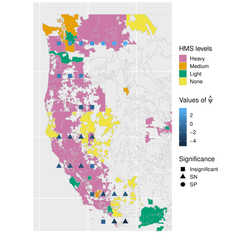
Figure 5: Estimated treatment effect $\hat{\psi}$ for the 27 locations in the Western US. The shapes of symbols denote whether $\hat{\psi}$ is insignificant, significantly negative (SN) or significantly positive (SN). The background color is the maximum daily HMS smoke density in each three-digit zip code. The units of effect is the number of symptoms.

To understand the spatial variation in the estimated treatment effect, we compare two populations for which the treatment effects are significant positive (SP, i.e., the lower bounds of the confidence intervals of $\psi$ are positive) versus significant negative (SN, i.e., the upper bounds of the confidence intervals of $\psi$ are negative). For easy comparison, we coarsen all baseline characteristics and two time-varying environmental variables (“Air quality yesterday” and “HMS”) as binary variables. For example, {Strongly disagree, Somewhat disagree, Neither agree nor disagree, Somewhat agree, Strongly agree} is converted into {Not strongly agree, Strongly agree}, represented by {0, 1} respectively. Then we fit logistic regression of each binary covariate on the indicator of belonging to the SP group $G_{{\rm SP}}$: logit$\{P(\text{covariate}=1)\}=\beta_{0}+\beta_{1}G_{{\rm SP}}$. Table 3 reports the covariates that have significant $\beta_{1}$ (p-values $<0.05$). Compared with the SN group, the users in the SP group experienced better air quality, less smoke, had more symptoms in the past, and had a stronger belief of the possibility to reduce the smoke exposure by themselves. Moreover, the SP population has a larger percentage of older, non-white, and higher educated people.

Table 3: Logistic regression results for the covariates which give the significant log odds ratio $\beta_{1}$.

Covariate	$\hat{\beta}_{1}$	P-value
Air quality yesterday ($1$ for $>$ Somewhat poor and $0$ otherwise)	1.3	0.00
HMS ($1$ for Heavy smoke density: $27\mu g/m^{3}$)	-1.0	0.00
Age ($1$ for $>$ 50 years old)	0.8	0.00
Race ($1$ for white)	-0.7	0.02
Education ($1$ for $>$ high school eduction)	0.9	0.04
Symptom 1 ($1$ for having health symptoms of class 1 in the past)	0.9	0.00
Strong agreement of the possibility to reduce smoke exposure	-0.5	0.03

7.3 Analysis for cities and national parks

We fit the local model to several cities including Spokane, Portland, Seattle, San Diego (SD), San Francisco (SF), Los Angeles (LA), Reno and Las Vegas (LV), as well as prominent national parks including Okanogan-Wenatchee National Forest (OW), Boise, Yosemite National Park (Yosemite), Death Valley National Park (DV), Joshua Tree National Park (Joshua), Lassen National Forest (Lassen). Figure 6 shows a forest plot of the point estimates and confidence intervals for $\psi$. The results are consistent with our findings in Section 7.2 that the users in the southwest locations have significant beneficial treatment effect while the users in the northwest do not. As shown in the right panel of Figure 6, the disjoint confidence intervals confirm there is a spatially varying treatment effect.

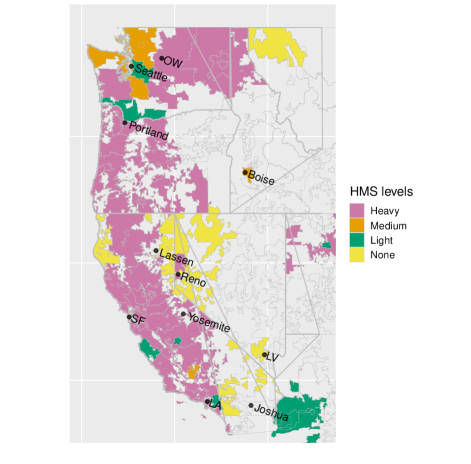
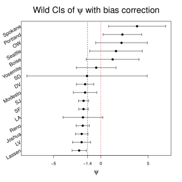
Figure 6: Location (left) and 95% confidence intervals of treatment effects (right) for the selected cities and national parks. The vertical black dash line is the global treatment effect estimate.

8 Discussion

It has become increasingly feasible to evaluate treatment and intervention strategies on public health as more health and activity data are collected via mobile phones, wearable devices, and smartphone applications. We establish a new framework of spatially and time-varying causal effect models. This provides a theoretical foundation to utilize emerging smartphone application data to draw causal inference of intervention on health outcomes. Our approach does not require specifying the full distribution of the covariate, treatment, and outcome processes. Moreover, our method achieves a double robustness property requiring the correct specification of either the model for the outcome mean or the model for the treatment process. The key underpinning assumption is sequential treatment randomization, which holds if all variables are measured that are related to both treatment and outcome. Although essential, it is not verifiable based on the observed data but rely on subject matter experts to assess its plausibility.

The goal of the Smoke Sense citizen science study is to engage the participants on the issue of wildfire smoke as a health risk and facilitate the adaptation of health-protective measures. Our new analysis framework reveals that there is a spatially varying health benefit and that the global model underestimates the treatment effect in areas with the highest exposure to wildland fire smoke. The exploratory analysis also suggests a beneficial treatment effect for people with a strong belief of health risks from smoke exposure. Thus, it is critically important to enhance the public awareness of the risks of smoke and the benefits of actions to reduce its exposure. This new knowledge obtained from the spatial analysis may also help Smoke Sense scientists and developers improve the app by targeting different people with different messaging.

There are several directions for future work. First, this work is limited to structural nested “mean” models for continuous or approximately continuous outcomes. It is important to continue the development of local causal models to accommodate different types of outcomes. For example, we can consider the structural nested failure time models for a time to event outcome (Yang, 2018). Second, the current framework relies on the sequential treatment randomization assumption. Yang and Lok (2017) assumed a bias function that quantifies the impact of unmeasured confounding and developed a modified estimator for the class of global SNMMs. Additional work is necessary to assess the impact of possible uncontrolled confounding for the new class of local SNMMs. Finally, with the app is continuously collecting more data from the users, one of the interesting future directions would be incorporating the covariates into the treatment effect model and estimate the optimal personalized behavior recommendations.

Disclaimer and conflicts of interest

The research described in this article has been reviewed by the Center for Public Health and Environmental Assessment, U.S. Environmental Protection Agency and approved for publication. Approval does not signify that the contents necessarily reflect the views and the policies of the Agency, nor does mention of trade names of commercial products constitute endorsement or recommendation for use. The authors declare that they have no conflict of interest.

Supplementary Material

Supplementary material online includes proofs, technical details and additional details for real data application.

References

- (1)
- Adibi (2014) Adibi, S. (2014). mHealth multidisciplinary verticals, CRC Press.
- Carroll et al. (1998) Carroll, R. J., Ruppert, D. and Welsh, A. H. (1998). Local estimating equations, J Am Stat Assoc 93: 214–227.
- Chakraborty and Moodie (2013) Chakraborty, B. and Moodie, E. E. (2013). Statistical Methods for Dynamic Treatment Regimes, Springer, New York.
- Fan and Gijbels (1996) Fan, J. and Gijbels, I. (1996). Local Polynomial Modelling and Its Applications, CRC Press, Chapman & Hall, London.
- Fotheringham et al. (2003) Fotheringham, A. S., Brunsdon, C. and Charlton, M. (2003). Geographically weighted regression: the analysis of spatially varying relationships, John Wiley & Sons.
- Galindo et al. (2001) Galindo, C. D., Liang, H., Kauermann, G. and Carrol, R. J. (2001). Bootstrap confidence intervals for local likelihood, local estimating equations and varying coefficient models, Statistica Sinica 11: 121–134.
- Gelfand et al. (2003) Gelfand, A. E., Kim, H.-J., Sirmans, C. and Banerjee, S. (2003). Spatial modeling with spatially varying coefficient processes, J Am Stat Assoc 98: 387–396.
- Holland (1986) Holland, P. W. (1986). Statistics and causal inference, J Am Stat Assoc 81: 945–960.
- Johnston et al. (2012) Johnston, F. H., Henderson, S. B., Chen, Y., Randerson, J. T., Marlier, M., DeFries, R. S., Kinney, P., Bowman, D. M. and Brauer, M. (2012). Estimated global mortality attributable to smoke from landscape fires, Environmental health perspectives 120(5): 695–701.
- Li et al. (2020) Li, W., Yang, S. and Han, P. (2020). Robust estimation for moment condition models with data missing not at random, Journal of Statistical Planning and Inference 207: 246–254.
- Pearl (2009) Pearl, J. (2009). Causality, 2 edn, Cambridge: Cambridge University Press.
- Rappold et al. (2019) Rappold, A., Hano, M., Prince, S., Wei, L., Huang, S., Baghdikian, C., Stearns, B., Gao, X., Hoshiko, S., Cascio, W. et al. (2019). Smoke sense initiative leverages citizen science to address the growing wildfire-related public health problem, GeoHealth 3: 443–457.
- Robins (1986) Robins, J. (1986). A new approach to causal inference in mortality studies with a sustained exposure period–application to control of the healthy worker survivor effect, Mathematical Modelling 7: 1393–1512.
- Robins (1994) Robins, J. M. (1994). Correcting for non-compliance in randomized trials using structural nested mean models, Comm. Statist. Theory Methods 23: 2379–2412.
- Robins (2000) Robins, J. M. (2000). Marginal structural models versus structural nested models as tools for causal inference, Statistical Models in Epidemiology, the Environment, and Clinical Trials, Vol. 11, Springer, New York, pp. 95–133.
- Robins et al. (1992) Robins, J. M., Blevins, D., Ritter, G. and Wulfsohn, M. (1992). G-estimation of the effect of prophylaxis therapy for pneumocystis carinii pneumonia on the survival of AIDS patients, Epidemiology 3: 319–336.
- Robins and Hernán (2009) Robins, J. M. and Hernán, M. A. (2009). Estimation of the causal effects of time-varying exposures, CRC Press, New York, pp. 553–599.
- Robins and Rotnitzky (1997) Robins, J. and Rotnitzky, A. (1997). Analysis of semi-parametric regression models with non-ignorable non-response, Stat Med 16: 81–102.
- Rubin (1976) Rubin, D. B. (1976). Inference and missing data, Biometrika 63: 581–592.
- Ruppert (1997) Ruppert, D. (1997). Empirical-bias bandwidths for local polynomial nonparametric regression and density estimation, J Am Stat Assoc 92: 1049–1062.
- Wang et al. (2014) Wang, S., Shao, J. and Kim, J. K. (2014). An instrumental variable approach for identification and estimation with nonignorable nonresponse, Statistica Sinica 24: 1097–1116.
- Yang (2018) Yang, S. (2018). Semiparametric efficient estimation of structural nested mean models with irregularly spaced observations, arXiv preprint arXiv:1810.00042 107: 123–136.
- Yang and Lok (2017) Yang, S. and Lok, J. J. (2017). Sensitivity analysis for unmeasured confounding in coarse structural nested mean models, Statistica Sinica 28: 1703–1723.