Classical capacities of memoryless but not identical quantum channels

Abstract

We study quantum channels that vary on time in a deterministic way, that is, they change in an independent but not identical way from one to another use. We derive coding theorems for the classical entanglement assisted and unassisted capacities. We then specialize the theory to lossy bosonic quantum channels and show the existence of contrasting examples where capacities can or cannot be drawn from the limiting behavior of the lossy parameter.

1 Introduction

Any physical process involves a state change and hence can be regarded as a quantum channel, i.e. a stochastic map on the set of density operators [1]. As such, it results quite naturally to characterize physical processes in terms of their ability to transmit information. Hence, much attention has been devoted to quantum channel capacities. They were, however, mostly confined to the assumption of channels acting in independent and identically distributed way over inputs. Only recently it has been started to go beyond this assumption [2].

A paradigm in this direction is provided by compound quantum channels where the map, though being the same over the uses, is initially randomly selected from a given set (with possibly infinite many elements)[3]. A more general situation is represented by arbitrarily varying quantum channels, where the sender and receiver must deal with further uncertainty. In fact, in this case, the map is randomly chosen (from a given set) at each use. Concerning this latter, wider class of quantum channels, the classical capacity was derived in [4] under the assumption of classical-quantum channels and then extended to the fully quantum channels in [5]. Instead, the entanglement-assisted classical capacity has been derived in [6]. In particular, in Ref.[4] it was proved that the average error classical capacity of a classical-quantum arbitrarily varying channel equals zero or else the random code capacity. Conditions for the latter case were found by using the elimination (or de-randomization) technique. Then, Ref.[5] showed how the random code capacity of a finite-dimensional quantum arbitrarily varying channel can be reduced to the capacity of a naturally associated compound channel by using permutation symmetry and de Finetti reduction. The technique used in Ref.[6] to prove a coding theorem for the entanglement-assisted classical capacity relies on the arguments used in Ref.[7] for finite-dimensional arbitrarily varying quantum channels. That is, capacity-achieving codes for general compound quantum channels were used. Next a variation of the so-called robustification and elimination techniques was borrowed from [8] as a method to extend the coding theorem to arbitrarily varying quantum channels.

Here we want to consider channels that are varying from one use to another, not in an arbitrary (random) way, but rather in a deterministic way. As such they cannot however be obtained as a particular case of arbitrarily varying quantum channels, because even if we concentrate the probability measure used therein to one item of the channels’ set, we recover the independent and identical distributed model. Instead, we would deal with independent but not identical channels and more specifically with classical information transmission through them. We shall derive the classical assisted and unassisted capacities formulae in a different way with respect to Refs.[4, 5, 6]. Namely, we shall employ position-based encoding [9, 10] and sequential decoding [11], which rely on quantum hypothesis testing and Berry-Esseen theorem [tools discussed in [12, 13, 14, 15] for finite-dimensional Hilbert spaces and in [16] for infinite-dimensional ones]. As a by-product, we obtain the validity of formulae also in the case of infinite-dimensional spaces. We then specialize the theory in this context by considering lossy bosonic quantum channels. The study of deterministic time-varying quantum channels is motivated by the fact that a determinist description is often taken for linear time-varying channels in wireless communication (see e.g. [17]), which is almost unexplored at the quantum level. Additionally, there are practical situations, of increasing interest for quantum communication, showing deterministically time-varying channels. One of these is provided by data transmission from a low-orbit satellite to a geostationary satellite or ground station. In such scenarios, the received signal power increases as the transmitting low-orbit satellite comes into view, and then decreases as it then departs, resulting in a communication link whose time variation is known to the sender and receiver (see e.g. [18]).

The paper is organized as follows. Preliminary notions, starting from smooth quantum relative entropy, are introduced in Section 2. In the core part of the paper, we will derive coding theorems for the classical entanglement assisted and unassisted capacities (Sections 3 and 4 respectively). We then specialize the theory to lossy bosonic quantum channels (Section 5) and show the existence of contrasting examples where capacities can or cannot be drawn from the limiting behavior of the lossy parameter (Section 6). Section 7 is for conclusions and Appendix A contains details on the deviation of smooth relative entropy from standard relative entropy.

2 Preliminaries

Let $\mathcal{H}$ be a separable Hilbert space, and let $\mathcal{T}(\mathcal{H})$ be a set of trace class linear operators acting on $\mathcal{H}$. A quantum channel $\mathcal{N}_{A\rightarrow B}$ is a completely positive trace preserving (CPTP) linear map from $\mathcal{T}(\mathcal{H}_{A})$ to $\mathcal{T}(\mathcal{H}_{B})$.

Suppose that we have an infinite sequence $\mathfrak{N}=\{{\cal N}_{k}^{A\to B}\}_{k}$ of quantum channels, known to both the sender and receiver before communication begins, whence referred to as deterministic. Here we want to address the issue of what are the classical capacities (entangled assisted and unassisted) of such a sequence of channels. To this end we cannot resort to the standard asymptotic theory that is valid for independent and identical channels. Rather, what we will do is to consider the one-shot capacity (see e.g. [12, 19, 10, 20, 21]) for the first $n$-items of the channels sequence and then let $n$ goes to infinity. In other words, $n$ items of the sequence are viewed as a single (larger) channel which will be used only once and the number of bits that can be transmitted through it with a given average error probability will be found. In doing so we need to introduce tools like smooth quantum relative entropy[12, 19].

A density operator on $\mathcal{H}$ is a positive linear operator with trace equal to one. Let us consider two density operators $\rho$ and $\sigma$ and assume that their spectral decompositions are given by

$$\rho=\sum_{x\in\mathcal{X}}\lambda_{x}P_{x}\quad\text{and}\quad\sigma=\sum_{y\in\mathcal{Y}}\mu_{y}Q_{y}\,,$$ (2.1)

where $\mathcal{X}$ and $\mathcal{Y}$ are countable index sets, $\{\lambda_{x}\}_{x\in\mathcal{X}}$ and $\{\mu_{y}\}_{y\in\mathcal{Y}}$ are probability distributions with $\sum_{x\in\mathcal{X}}\lambda_{x}=\sum_{y\in\mathcal{Y}}\mu_{y}=1$, and $P_{x},Q_{y}$ are projections such that $\sum_{x\in\mathcal{X}}P_{x}=\sum_{y\in\mathcal{Y}}Q_{y}=I$.

Given a Positive Operator Valued Measure (POVM) with two elements, $\Pi$ and $I-\Pi$, aimed at distinguishing $\rho$ from $\sigma$, we consider a smoothed version of quantum relative entropy defined as the negative logarithm of the minimum probability that the ‘test’ $\Pi$ will fail on state $\sigma$, under the constraint that its failure probability on state $\rho$ is not larger than $\varepsilon\in(0,1)$, that is [12, 19]

$$D_{H}^{\varepsilon}(\rho\|\sigma)\equiv\sup_{0\leq\Pi\leq I,\,\operatorname{Tr}(\Pi\rho)\geq 1-\varepsilon}\left[-\log\operatorname{Tr}(\Pi\sigma)\right]\,.$$ (2.2)

Throughout this paper $\log$ stands for $\log_{2}$.

The quantum relative entropy [22], its variance [15, 14, 13] and the $T$ quantity are respectively defined as [15, 14, 13]:

$$D(\rho\|\sigma)\equiv\sum_{x\in\mathcal{X},y\in\mathcal{Y}}\lambda_{x}\operatorname{Tr}(P_{x}Q_{y})\log\left(\frac{\lambda_{x}}{\mu_{y}}\right)\,,$$ (2.3)

$$V(\rho\|\sigma)\equiv\sum_{x\in\mathcal{X},y\in\mathcal{Y}}\lambda_{x}\operatorname{Tr}(P_{x}Q_{y})\left(\log\left(\frac{\lambda_{x}}{\mu_{y}}\right)-D(\rho\|\sigma)\right)^{2}\,,$$ (2.4)

$$T(\rho\|\sigma)\equiv\sum_{x\in\mathcal{X},y\in\mathcal{Y}}\lambda_{x}\operatorname{Tr}(P_{x}Q_{y})\left|\log\left(\frac{\lambda_{x}}{\mu_{y}}\right)-D(\rho\|\sigma)\right|^{3}\,.$$ (2.5)

For given density operators $\rho$ and $\sigma$ satisfying

$$D(\rho\|\sigma),V(\rho|\sigma)\,\,\text{and}\,\,T(\rho\|\sigma)<\infty\,,$$ (2.6)

we have the following expansion

$$D_{H}^{\varepsilon}\left(\rho^{\otimes n}\|\sigma^{\otimes n}\right)=nD(\rho\|\sigma)+\sqrt{nV(\rho\|\sigma)}\Phi^{-1}(\varepsilon)+O(\log n)\,,$$ (2.7)

where

$$\Phi(a)\equiv\frac{1}{\sqrt{2\pi}}\int_{-\infty}^{a}\operatorname{exp}\left(-\frac{x^{2}}{2}\right)dx,\qquad\Phi^{-1}(\varepsilon)=\sup\{a\in\mathds{R}|\Phi(a)<\varepsilon\}\,.$$ (2.8)

Relation  (2.7) was proven for finite dimensional Hilbert spaces in  [15, 14]. For infinite-dimensional separable Hilbert spaces, the inequality $\leq$ was proven in [23, 13], while the inequality $\geq$ was shown in [16]. In Appendix A, we generalize it as follows

$$D_{H}^{\varepsilon}\left(\bigotimes_{i=1}^{n}\rho_{i}\Bigg{\|}\bigotimes_{i=1}^{n}\sigma_{i}\right)=\sum_{i=1}^{n}D(\rho_{i}\|\sigma_{i})+\sqrt{\sum_{i=1}^{n}V(\rho_{i}\|\sigma_{i})}\,\Phi^{-1}\!\left(\varepsilon\right)+O(\log n)\,,$$ (2.9)

where $\rho_{i}$’s and $\sigma_{i}$’s are density operators acting on $\mathcal{H}$ with the additional condition

$$\lim_{n\to\infty}\frac{6\sum_{i=1}^{n}\left(T(\rho_{i}\|\sigma_{i})\right)}{\sqrt{\left(\sum_{i=1}^{n}V\left(\rho_{i}\|\sigma_{i}\right)\right)^{3}}}=0\,.$$ (2.10)

3 Entanglement assisted classical capacity

In this Section we present the coding theorem for the entanglement assisted classical capacity of a deterministic sequence of independent channels $\mathfrak{N}=\{{\cal N}_{k}^{A\to B}\}_{k}$.

Suppose that channels $\mathfrak{N}$ connect a sender Alice to a receiver Bob and they can share an arbitrary quantum state $\rho_{R^{n}A^{n}}$ before using the first $n$ items of $\mathfrak{N}$. Here the system $R$ (resp. $A$) is considered as accessible to Bob (resp.) Alice. For positive integers $n$ and $M$, and $\varepsilon\in\left[0,1\right]$, an $(n,M,\varepsilon)$ code for entanglement-assisted classical communication consists of the resource state $\rho_{R^{n}A^{n}}$ and a set $\{\mathcal{E}_{A^{n}\rightarrow A^{n}}^{m}\}_{m\in\mathcal{M}}$ of encoding channels, where $\left|\mathcal{M}\right|=M$. It also consists of a decoding POVM $\left\{\Lambda_{R^{n}B^{n}}^{m}\right\}_{m\in\mathcal{M}}$ satisfying the following condition:

$$\frac{1}{M}\sum_{m\in\mathcal{M}}\operatorname{Tr}\{\left(I_{R^{n}B^{n}}-\Lambda_{R^{n}B^{n}}^{m}\right)\otimes_{k=1}^{n}\mathcal{N}_{k}^{A\to B}(\mathcal{E}_{A^{n}\rightarrow A^{n}}^{m}(\rho_{R^{n}A^{n}}))\}\leq\varepsilon\,,$$ (3.1)

which we interpret as saying that the average error probability is no larger than $\varepsilon$, when using the entanglement-assisted code described above.

The entanglement-assisted classical capacity of the first $n$ items of $\mathfrak{N}$, denoted by $C_{{E}}(\mathfrak{N},n,\varepsilon)$, is equal to the largest value of $\frac{1}{n}\log M$ (bits per channel use) for which there exists an $\left(n,M,\varepsilon\right)$ entanglement-assisted code as described above. The entanglement assisted classical capacity for $\mathfrak{N}$ is defined by

$$C_{{E}}(\mathfrak{N})\equiv\lim_{\varepsilon\to 0}\lim_{n\to\infty}C_{{E}}(\mathfrak{N},n,\varepsilon)\,.$$ (3.2)

Theorem 1

Given a deterministic sequence of independent channels $\mathfrak{N}=\{{\cal N}_{k}^{A\to B}\}_{k}$, the entanglement assisted classical capacity results

$${C_{E}}(\mathfrak{N})=\lim_{n\to\infty}\frac{1}{n}\left[\max_{\rho_{RA}}\sum_{k=1}^{n}D\left({\cal N}_{k}^{A\to B}(\rho_{RA})\Big{\|}\rho_{R}\otimes{\cal N}_{k}^{A\to B}(\rho_{A})\right)\right],$$ (3.3)

where $\rho_{RA}$ is a resource entangled state shared by Alice and Bob.

To prove the Theorem, we will resort to position-based encoding and sequential decoding strategy. In other words, Alice and Bob are supposed to share $M$ resource entangled states $\rho_{R_{i}A_{i}}$, $i=1,\cdots,M$ where Bob has $R$ systems and Alice has $A$ systems. If Alice wants to transmit the message $m$ through the channel $\mathcal{N}^{A\to B}$, simply selects the $m$’s state in her systems and sends it through the channel so that the marginal state of Bob systems is as follows

$$\rho_{R_{1}}\otimes\cdots\otimes\rho_{R_{m-1}}\otimes\mathcal{N}^{A_{m}\rightarrow B}(\rho_{R_{m}A_{m}})\otimes\rho_{R_{m+1}}\otimes\cdots\otimes\rho_{R_{M}}\,.$$ (3.4)

Bob then to determine which message Alice transmitted, introduces $M$ auxiliary probe systems in the state $|0\rangle\langle 0|$, so that his overall state is

$$\omega_{R^{M}BP^{M}}^{m}\equiv\rho_{R_{1}}\otimes\cdots\otimes\rho_{R_{m-1}}\otimes\mathcal{N}^{A_{m}\rightarrow B}(\rho_{R_{m}A_{m}})\otimes\rho_{R_{m+1}}\otimes\cdots\otimes\rho_{R_{M}}\otimes|0\rangle\langle 0|_{P_{1}}\otimes\cdots\otimes|0\rangle\langle 0|_{P_{M}}\,.$$ (3.5)

He next performs the binary measurements $\{\Pi_{R_{i}B_{m}P_{i}},\hat{\Pi}_{R_{i}B_{m}P_{i}}\equiv I_{R_{i}B_{m}P_{i}}-\Pi_{R_{i}B_{m}P_{i}}\}$, sequentially, in the order $i=1$, $i=2$, etc. With this strategy, the probability that he decodes the $m$th message correctly is given by

$$\operatorname{Tr}\{\Pi_{R_{m}BP_{m}}\hat{\Pi}_{R_{m-1}BP_{m-1}}\cdots\hat{\Pi}_{R_{1}BP_{1}}\omega_{R^{M}BP^{M}}^{m}\hat{\Pi}_{R_{1}BP_{1}}\cdots\hat{\Pi}_{R_{m-1}BP_{m-1}}\}\,.$$ (3.6)

Applying the “quantum union bound" [16], we can bound the complementary probability (error probability)

$$p_{\text{e}}(m) \equiv 1-\operatorname{Tr}\{\Pi_{R_{m}BP_{m}}\hat{\Pi}_{R_{m-1}BP_{m-1}}\cdots\hat{\Pi}_{R_{1}BP_{1}}\omega_{R^{M}BP^{M}}^{m}\hat{\Pi}_{R_{1}BP_{1}}\cdots\hat{\Pi}_{R_{m-1}BP_{m-1}}\}\,.$$ (3.7)

More specifically, by [16, Theorem 5.1] $p_{\text{e}}(m)\leq\varepsilon$ holds for all $m$, when

$$\log M=D_{H}^{\varepsilon-\eta}\left(\mathcal{N}(\rho_{RB})\|\rho_{R}\otimes\mathcal{N}(\rho_{A})\right)-\log(4\varepsilon/\eta^{2}),$$ (3.8)

where $\eta\in(0,\varepsilon)$ and $\varepsilon\in(0,1)$. Now, we are going to use this relation to provide a lower bound on the position-based encoding and sequential decoding for the entangled assisted classical capacity of the channel sequence $\{\mathcal{N}_{k}^{A\to B}\}_{k}$.

Lemma 2

A message $m\in{\cal M}$ can be sent through the channels $\bigotimes_{k=1}^{n}\mathcal{N}_{k}$ with $p_{\text{e}}(m)\leq\varepsilon$ by choosing

$$\log M =\sum_{k=1}^{n}D\left({\cal N}^{A\to B}_{k}(\rho_{RA})\Big{\|}\rho_{R}\otimes{\cal N}^{A\to B}_{k}(\rho_{A})\right)$$

$$+\sqrt{\sum_{k=1}^{n}V\left({\cal N}^{A\to B}_{k}(\rho_{RA})\big{\|}\rho_{R}\otimes{\cal N}^{A\to B}_{k}(\rho_{A})\right)}\Phi^{-1}\left(\varepsilon-\frac{1}{\sqrt{n}}\right)+O(\log n)\,.$$ (3.9)

Proof. By replacing $\mathcal{N}^{A\to B}$ with $\bigotimes_{k=1}^{n}\mathcal{N}_{k}^{A\to B}$ and letting $\Lambda_{R_{i}^{n}B^{n}}^{n}$ be a measurement operator such that

$$\Lambda_{R_{i}^{n}B^{n}}^{n}=\operatorname{argmax}_{\Lambda}\left(D_{H}^{\varepsilon}\left(\bigotimes_{k=1}^{n}\mathcal{N}^{A_{i}\rightarrow B}_{k}(\rho_{R_{i}A_{i}})\Big{\|}\bigotimes_{k=1}^{n}\rho_{R_{i}}\otimes\mathcal{N}^{A_{i}\rightarrow B}_{k}(\rho_{A_{i}})\right)\right)\,,$$ (3.10)

we can get from (3.8)

$$\log{M}={D_{H}^{\varepsilon-\eta}\left(\bigotimes_{k=1}^{n}\mathcal{N}^{A\rightarrow B}_{k}(\rho_{RA})\Big{\|}\bigotimes_{k=1}^{n}\rho_{R}\otimes\mathcal{N}^{A\rightarrow B}_{k}(\rho_{A})\right)}-\log\left(\frac{4\varepsilon}{\eta^{2}}\right)\,.$$ (3.11)

Next, setting $\eta=1/\sqrt{n}$, with the second order asymptotic relation (2.9) we arrive at

$$\log M =\sum_{k=1}^{n}D\left({\cal N}^{A\to B}_{k}(\rho_{RA})\big{\|}\rho_{R}\otimes{\cal N}^{A\to B}_{k}(\rho_{A})\right)+$$

$$+\sqrt{\sum_{k=1}^{n}V\left({\cal N}^{A\to B}_{k}(\rho_{RA})\|\rho_{R}\otimes{\cal N}^{A\to B}_{k}(\rho_{A})\right)}\Phi^{-1}\left(\varepsilon-\frac{1}{\sqrt{n}}\right)+O(\log n)\,,$$ (3.12)

with the condition

$$\lim_{n\to\infty}\frac{6\sum_{k=1}^{n}\left[T\left({\cal N}^{A\to B}_{k}(\rho_{RA})\|\rho_{R}\otimes{\cal N}^{A\to B}_{k}(\rho_{A})\right)\right]}{\sqrt{\left[\sum_{k=1}^{n}V\left(\mathcal{N}^{A\rightarrow B}_{k}(\rho_{RA})\|\rho_{R}\otimes\mathcal{N}^{A\rightarrow B}_{k}(\rho_{A})\right)\right]^{3}}}=0\,.$$ (3.13)

 

Proof. Theorem 1. The direct part is based on the result of Lemma 2 which provides a lower bound for the capacity, namely

$${n\,C_{E}}(\mathfrak{N},n,\varepsilon) \geq\max_{\rho_{RA}}\sum_{k=1}^{n}D\left({\cal N}^{A\to B}_{k}(\rho_{RA})\big{\|}\rho_{R}\otimes{\cal N}^{A\to B}_{k}(\rho_{A})\right)$$

$$+\sqrt{\sum_{k=1}^{n}V\left({\cal N}^{A\to B}_{k}(\rho_{RA})\|\rho_{R}\otimes{\cal N}^{A\to B}_{k}(\rho_{A})\right)}\Phi^{-1}\left(\varepsilon-\frac{1}{\sqrt{n}}\right)+O(\log n)\,.$$ (3.14)

For the converse part, since the channels are independent, though not identical, it is like to have them used in parallel, hence

$${n\,C_{E}}(\mathfrak{N},n,\varepsilon)\leq\max_{\rho_{RA}}\sum_{k=1}^{n}D\left({\cal N}_{k}^{A\to B}(\rho_{RA})\big{\|}\rho_{R}\otimes{\cal N}_{k}^{A\to B}(\rho_{A})\right).$$ (3.15)

 

Remark 3

From Eqs.(3) and (3.15) it is evident that, by taking the limit $n\to\infty$, the dependence on $\epsilon$ disappears. Hence the subsequent limit $\epsilon\to 0$ results superfluous.

Remark 4

For arbitrarily varying quantum channel, Ref. [6], the encoding depends on the dimension of input Hilbert space and so the capacity formula cannot work in the infinite dimensional case, while here we do not have such a restriction.

4 Unassisted classical capacity

This Section is devoted to the coding theorem for the unassisted classical capacity of a deterministic sequence of independent channel $\mathfrak{N}=\{{\cal N}_{k}^{A\to B}\}_{k}$.

Suppose that channels $\mathfrak{N}$ connect a sender Alice to a receiver Bob. For positive integers $n$ and $M$, and $\varepsilon\in\left[0,1\right]$, an $(n,M,\varepsilon)$ code for classical communication consists of a set $\{\rho_{A^{n}}^{m}\}$ of separable quantum states across systems $A_{k}$, which are called quantum codewords, and where $\left|\mathcal{M}\right|=M$. It also consists of a decoding POVM $\left\{\Lambda_{B^{n}}^{m}\right\}_{m\in\mathcal{M}}$ satisfying the following condition:

$$\frac{1}{M}\sum_{m\in\mathcal{M}}\operatorname{Tr}\{\left(I_{B^{n}}-\Lambda_{B^{n}}^{m}\right)\otimes_{k=1}^{n}\mathcal{N}_{k}^{A\to B}(\rho_{A^{n}}^{m})\}\leq\varepsilon\,,$$ (4.1)

which we interpret as saying that the average error probability is no larger than $\varepsilon$, when using the quantum codewords and decoding POVM described above.

The unassisted classical capacity with separable inputs of the first $n$ items of $\mathfrak{N}$, denoted by $C(\mathfrak{N},n,\varepsilon)$, is equal to the largest value of $\frac{1}{n}\log M$ (bits per channel use) for which there exists an $\left(n,M,\varepsilon\right)$ code as described above. The unassisted classical capacity for $\mathfrak{N}$ is defined by

$$C(\mathfrak{N})\equiv\lim_{\varepsilon\to 0}\lim_{n\to\infty}C(\mathfrak{N},n,\varepsilon)\,.$$ (4.2)

Theorem 5

Given a deterministic sequence of independent channel $\mathfrak{N}=\{{\cal N}_{k}^{A\to B}\}_{k}$, the unassisted classical capacity with separable inputs results

$$C(\mathfrak{N})=\lim_{n\to\infty}\frac{1}{n}\left[\max_{\rho_{X^{n}A^{n}}}\sum_{k=1}^{n}D\left({\cal N}_{k}^{A\to B}(\rho_{XA_{k}})\Big{\|}\rho_{X}\otimes{\cal N}_{k}^{A\to B}(\rho_{A_{k}})\right)\right]\,,$$ (4.3)

where

$$\rho_{X^{n}A^{n}}=\sum_{x^{n}\in{\cal X}^{n}}p(x^{n})\,|x^{n}\rangle\langle x^{n}|\otimes\rho_{A^{n}}^{x^{n}}$$ (4.4)

is a classical-quantum state, with $|x^{n}\rangle\in{\cal H}_{X}^{\otimes n}$ orthonormal states (being ${\cal H}_{X}$ a separable Hilbert space) and $\rho_{A^{n}}^{x^{n}}=\left(\rho_{A_{1}}^{x_{1}}\otimes\ldots\otimes\rho^{x_{n}}_{A_{n}}\right)$.

Given a classical-quantum channel $x\rightarrow\rho_{B}^{x}$, we know from [24] that there exists an encoding and position-based decoding for choosing

$$\log M=D_{H}^{\varepsilon-\eta}\left(\rho_{XB}\|(\rho_{X}\otimes\rho_{B})\right)-\log(4\varepsilon/\eta^{2}),$$ (4.5)

where $\eta\in(0,\varepsilon)$, $\varepsilon\in(0,1)$ and

$$\rho_{XB}=\sum_{x}p(x)|x\rangle\langle x|\otimes\rho_{B}^{x}\,,$$ (4.6)

with $\rho_{B}^{x}\equiv{\cal N}(\rho_{A}^{x})$. In other words, there exist an encoding $m\rightarrow\rho_{A}^{x_{m}}$ and position-based POVM $\{\Lambda_{B}^{x_{m}}\}_{m=1}^{M}$ as decoder such that, according to (4.1), and together with [16, Theorem 5.1], $p_{\text{e}}(m)\leq\varepsilon$ holds for all $m\in{\cal M}$.

Lemma 6

A message $m\in{\cal M}$ can be sent through the channels $\bigotimes_{k=1}^{n}\mathcal{N}_{k}$ with $p_{\text{e}}(m)\leq\varepsilon$ by choosing

$$\log M =\sum_{k=1}^{n}D\left({\cal N}^{A\to B}_{k}(\rho_{RA})\big{\|}\rho_{R}\otimes{\cal N}^{A\to B}_{k}(\rho_{A})\right)$$

$$+\sqrt{\sum_{k=1}^{n}V\left({\cal N}^{A\to B}_{k}(\rho_{RA})\|\rho_{R}\otimes{\cal N}^{A\to B}_{k}(\rho_{A})\right)}\Phi^{-1}\left(\varepsilon-\frac{1}{\sqrt{n}}\right)+O(\log n)\,.$$ (4.7)

Proof. If we replace $\rho_{XB}$ with $\bigotimes_{i=1}^{n}\rho_{XB_{i}}$ in Eq.(4.5), then we have

$$\log M{=}D_{H}^{\varepsilon-\eta}\left(\bigotimes_{k=1}^{n}\rho_{XB_{k}}\Big{\|}\bigotimes_{k=1}^{n}(\rho_{X}\otimes\rho_{B_{k}})\right)-\log(4\varepsilon/\eta^{2})\,.$$ (4.8)

As a consequence, following the arguments of Lemma 2, we can get

$$\log M(\varepsilon){=}\sum_{k=1}^{n}D\left(\rho_{XB_{k}}\|\rho_{X}\otimes\rho_{B_{k}}\right)+\sqrt{\sum_{k=1}^{n}V\left(\rho_{XB_{k}}\|\rho_{R}\otimes\rho_{B_{k}}\right)}\Phi^{-1}\left(\varepsilon-\frac{1}{\sqrt{n}}\right)+O(\log n)\,,$$ (4.9)

with the condition

$$\lim_{n\to\infty}\frac{6\sum_{k=1}^{n}\left(T\left(\rho_{XB_{k}}\|\rho_{X}\otimes\rho_{B_{k}}\right)\right)}{\sqrt{\left(\sum_{k=1}^{n}V\left(\rho_{XB_{k}}\|\rho_{X}\otimes\rho_{B_{k}}\right)\right)^{3}}}=0\,.$$ (4.10)

 

Proof. Theorem 5. The direct part is based on the result of Lemma 6 which provides a lower bound for the capacity, namely

$$n\,C(\mathfrak{N},n,\varepsilon)\geq\max_{\rho_{XA^{n}}}\left[\sum_{k=1}^{n}D\left(\rho_{XB_{k}}\|\rho_{X}\otimes\rho_{B_{k}}\right)+\sqrt{\sum_{k=1}^{n}V\left(\rho_{XB_{k}}\|\rho_{R}\otimes\rho_{B_{k}}\right)}\Phi^{-1}\left(\varepsilon-\frac{1}{\sqrt{n}}\right)+O(\log n)\right]\,.$$ (4.11)

For the converse part, since the channels are independent, though not identical, it is like to have them used in parallel, hence from the Holevo bound we have

$$n\,C(\mathfrak{N},n,\varepsilon)\leq\max_{\rho_{XA^{n}}}\sum_{k=1}^{n}D\left(\rho_{XB_{k}}\|\rho_{X}\otimes\rho_{B_{k}}\right).$$ (4.12)

 

Remark 7

From Eqs.(4.11) and (4.12) it is evident that, by taking the limit $n\to\infty$, the dependence on $\epsilon$ disappears. Hence the subsequent limit $\epsilon\to 0$ results superfluous.

Remark 8

We have employed the hypothesis testing based on the Berry-Esseen theorem to get the formula (4.9) as average of relative entropies of single channels. In contrast for arbitrarily varying quantum channels, Ref.[4], it was used the sum of $n$ entropies greater than $n$ times the smallest of them. Furthermore, in case we consider a finite dimensional Hilbert space, and parallel the error bound (4.9) with that obtained for arbitrarily varying quantum channels [4], we note that the former only depends on the number of channel uses, while the latter also on the size of channels’ set.

5 Memoryless but not identical Gaussian lossy channels

Since the coding Theorems 1 and 5 were derived without any restriction on the dimensionality of Hilbert spaces, they can be straightforwardly applied to continuous variable (bosonic) quantum channels.

We shall focus on a sequence of Gaussian lossy channels (each acting on a single bosonic mode) $\{{\cal N}_{\eta_{k}}\}_{k=1}^{\infty}$, where $\eta_{k}\in(0,1)$ is the trasmissivity characterizing the $k$th channel. As customary we shall also consider an average energy $N$ per channel use, so to have the constraint

$$\sum_{k=1}^{n}N_{k}=nN\,,$$ (5.1)

on the effective energy $N_{k}$ employed at $k$th use.

5.1 Entangled assisted classical capacity

We consider Alice and Bob sharing $M$ two-mode squeezed state each with photon mean number $N_{k}$. We want to see how the capacity resulting from Theorem 1 is approached over channel uses.

In Ref.[25] it has been shown that

$$D\left({\cal N}_{A\to B}^{k}(\rho_{RA})\|\rho_{R}\otimes{\cal N}_{A\rightarrow B}^{k}(\rho_{A})\right)=g(N_{k})+g(\eta_{k}N_{k})-g((1-\eta_{k})N_{k})\,,$$ (5.2)

where $g(x)\equiv(x+1)\log(x+1)-x\log x$. In addition, the quantum relative entropy variance is computed in [13] as

$$V\left({\cal N}_{A\to B}^{k}(\rho_{RA})\|\rho_{R}\otimes{\cal N}_{A\to B}^{k}(\rho_{A})\right) =(1-\eta_{k})N_{k}\left((1-\eta_{k})N_{k}+1\right)\left[\log\left(1+\frac{1}{(1-\eta_{k})N_{k}}\right)\right]^{2}$$

$$-2(1-\eta_{k})N_{k}(N_{k}+1)\log\left(1+\frac{1}{(1-\eta_{k})N_{k}}\right)\log\left(1+\frac{1}{N_{k}}\right)$$

$$+N_{k}(N_{k}+1)\left[\log\left(1+\frac{1}{N_{k}}\right)\right]^{2}\,.$$ (5.3)

According to Theorem 1 and (5.2) we now need to maximize the quantity

$$\sum_{k=1}^{n}\left[g\left(N_{k}\right)+g\left(\eta_{k}N_{k}\right)-g\left((1-\eta_{k})N_{k}\right)\right],$$ (5.4)

with respect to $N_{k}$. This amounts to set

$$\delta\left\{\text{Eq.\eqref{sumgV}}\right\}=\sum_{k=1}^{n}\Bigg{[} g^{\prime}\left(N_{k}\right)+\eta_{k}g^{\prime}\left(\eta_{k}N_{k}\right)-(1-\eta_{k})g^{\prime}\left(({1-}\-\eta_{k})N_{k}\right)\Bigg{]}\delta N_{k}=0,$$ (5.5)

where $g^{\prime}$ stands for the derivative of $g$ with respect to its argument. From the energy constraint (5.1) we further have

$$\delta\left\{\sum_{k=1}^{n}N_{k}\right\}=\sum_{k=1}^{n}\delta N_{k}=0.$$ (5.6)

Using a Lagrange multiplier $\beta$ we get

$$\sum_{k=1}^{n}\Bigg{[}g^{\prime}\left(N_{k}\right)+\eta_{k}g^{\prime}\left(\eta_{k}N_{k}\right)-(1-\eta_{k})g^{\prime}\left(({1-}\-\eta_{k})N_{k}\right)-\beta\Bigg{]}\delta N_{k}=0.$$ (5.7)

Solving the set of $n+1$ equations

$$\left\{\begin{array}[]{cl}g^{\prime}\left(N_{k}\right)+\eta_{k}g^{\prime}\left(\eta_{k}N_{k}\right)-(1-\eta_{k})g^{\prime}\left(({1-}\-\eta_{k})N_{k}\right)-\beta&=0\\ \\ \sum_{k=1}^{n}N_{k}&=nN\end{array}\right.,$$ (5.8)

allows us to find the $N_{k}$ and $\beta$ giving

$$n\,\overline{C_{E}}(\{{\cal N}_{\eta_{k}}\},n)\equiv\max_{N_{k}}\sum_{k=1}^{n}\left[g\left(N_{k}\right)+g\left(\eta_{k}N_{k}\right)-g\left((1-\eta_{k})N_{k}\right)\right].$$ (5.9)

where $\overline{C_{E}}(\{{\cal N}_{\eta_{k}}\},n)$ denotes the upper bound on $C_{E}(\{{\cal N}_{\eta_{k}}\},n,\epsilon)$. Clearly $\lim_{n\to\infty}C_{E}(\{{\cal N}_{\eta_{k}}\},n,\epsilon)=C_{E}(\{{\cal N}_{\eta_{k}}\})$.

The variance of the quantum relative entropy $\overline{C_{E}}(\{{\cal N}_{\eta_{k}}\},n)$ can be obtained by means of (5.1) as

$$\frac{1}{n^{2}}\sum_{k=1}^{n}V\left({\cal N}_{A\to B}^{k}(\rho_{RA})\|\rho_{R}\otimes{\cal N}_{A\to B}^{k}(\rho_{A})\right).$$ (5.10)

5.2 Unassisted classical capacity

Here we want to see how the capacity resulting from Theorem 5 is approached over channel uses.

From Ref. [26], we know that

$$D(\rho_{XB_{k}}\|\rho_{X}\otimes\rho_{B_{k}})=g(\eta_{k}N_{k})\,,$$ (5.11)

and

$$V(\rho_{XB_{k}}\|\rho_{X}\otimes\rho_{B_{k}})=\eta_{k}N_{k}(\eta_{k}N_{k}+1)\left[\log\left(\eta_{k}N_{k}+1\right)-\log\left(\eta_{k}N_{k}\right)\right]^{2}\,.$$ (5.12)

Then, according to Theorem 1 and (5.2) we now need to maximize the quantity

$$\sum_{k=1}^{n}g(\eta_{k}N_{k}),$$ (5.13)

with respect to $N_{k}$.

Proceeding like in the previous section, using a Lagrange multiplier $\beta$ and imposing (5.1), we get

$$\left\{\begin{array}[]{cl}g^{\prime}\left(N_{k}\right)-\beta&=0\\ \\ \sum_{k=1}^{n}N_{k}&=nN\end{array}\right..$$ (5.14)

Solving this set of $n+1$ equations allows us to find the $N_{k}$ and $\beta$ giving

$$n\,\overline{C}(\{{\cal N}_{\eta_{k}}\},n)\equiv\max_{N_{k}}\sum_{k=1}^{n}\left[g\left(N_{k}\right)\right].$$ (5.15)

where $\overline{C}(\{{\cal N}_{\eta_{k}}\},n)$ denotes the upper bound on $C(\{{\cal N}_{\eta_{k}}\},n,\epsilon)$. Clearly $\lim_{n\to\infty}\overline{C}(\{{\cal N}_{\eta_{k}}\},n)=C(\{{\cal N}_{\eta_{k}}\})$.

The variance of the quantum relative entropy $\overline{C}(\{{\cal N}_{\eta_{k}}\},n)$ can be obtained by means of (5.12) as

$$\frac{1}{n^{2}}\sum_{k=1}^{n}V(\rho_{XB_{k}}\|\rho_{X}\otimes\rho_{B_{k}}).$$ (5.16)

6 Examples

We now apply the results of Sec.5 to some specific cases study, i.e. specific sequences of lossy channels.

6.1 Example 1

Consider

$$\eta_{k}=\underline{\eta}+\overline{\eta}e^{-(k-1)^{2}/\Delta},\qquad 0<\underline{\eta},\overline{\eta}<\frac{1}{2}\,.$$ (6.1)

After a transient (whose extension is determined by $\Delta$) the channel reaches a transmissivity $\underline{\eta}$ (see Fig.1). The distribution of input energy shows a similar behavior to transmissivity (see Fig.1). Note however that the sequence of input energies $\{N_{k}^{(n)}\}_{k}$ depends on the number $n$ of channel uses.

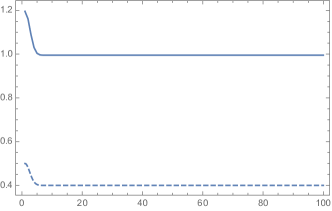
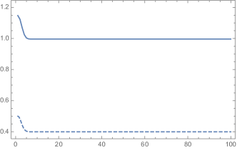
Figure 1: Q

uantities $\eta_{k}$ (dashed line) and $N_{k}^{(n)}$ (solid line) vs $k$ for $n=100$. On the left (resp. right) is the case for entanglement assisted (resp. unassisted) classical communication. It is $\Delta=5$. The values of other parameters are $\underline{\eta}=0.4,\overline{\eta}=0.1,N=1$.

For this example the capacity $C_{E}(\{{\cal N}_{\eta_{k}}\})$ can be guessed by simply computing $\overline{C_{E}}(\{{\cal N}_{\lim_{k\to\infty}\eta_{k}}\},n=1)$ (see Fig.2 left). Analogous argument holds true for $C(\{{\cal N}_{\eta_{k}}\})$, i.e. it can be guessed by simply computing $\overline{C}(\{{\cal N}_{\lim_{k\to\infty}\eta_{k}}\},n=1)$ (see Fig.2 right).

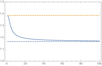
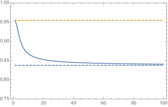
Figure 2: (Left) $\overline{C_{E}}(\{{\cal N}_{\eta_{k}}\},n)$ vs $n$ for $\Delta=5$ (solid line). The bottom (resp. top) dashed line represents the capacity $g(N)+g(\underline{\eta}N)-g((1-\underline{\eta})N)$ (resp. $g(N)+g((\underline{\eta}+\overline{\eta})N)-g((1-(\underline{\eta}+\overline{\eta}))N)$). (Right) $\overline{C}(\{{\cal N}_{\eta_{k}}\},n)$ vs $n$ for $\Delta=5$ (solid line). The bottom (resp. top) dashed line represents the capacity $g(\underline{\eta}N)$ (resp. $g((\underline{\eta}+\overline{\eta})N)$). The values of other parameters are $\underline{\eta}=0.4,\overline{\eta}=0.1,N=1$.

In Fig.3 we report the variances (5.10) and (5.16) as functions of $n$. As one can see the variance of $\overline{C_{E}}(\{{\cal N}_{\eta_{k}}\},n)$ converges faster than that of $\overline{C}(\{{\cal N}_{\eta_{k}}\},n)$.

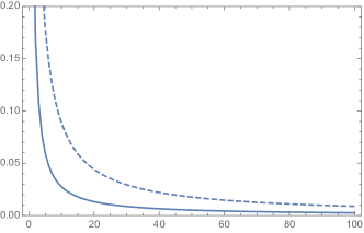
Figure 3: Variance of $\overline{C_{E}}(\{{\cal N}_{\eta_{k}}\},n)$ (solid line) and of $\overline{C}(\{{\cal N}_{\eta_{k}}\},n)$ (dashed line) vs $n$ for $\Delta=5,\underline{\eta}=0.4,\overline{\eta}=0.1,N=1$.

6.2 Example 2

Consider

$$\eta_{k}=\underline{\eta}+\overline{\eta}\left|\sin\left(\frac{k-1}{\Delta}+\frac{\pi}{2}\right)\right|,\qquad 0<\underline{\eta},\overline{\eta}<\frac{1}{2}.$$ (6.2)

In this case we have an oscillatory behavior of $\eta_{k}$ (whose frequency is determined by $\Delta$), as can be seen in Fig.4. The distribution of input energy still follows the behavior of transmissivity.

Figure 4: Quantities $\eta_{k}$ (dashed line) and $N_{k}^{(n)}$ (solid line) vs $k$ for $n=100$. On the left (resp. right) is the case for entanglement assisted (resp. unassisted) classical communication. It is $\Delta=5$. The values of other parameters are $\underline{\eta}=0.4,\overline{\eta}=0.1,N=1$.

In this case the capacities cannot be guessed by the $\lim_{k\to\infty}\eta_{k}$, because this latter does not exist, however the bound $\overline{C_{E}}(\{{\cal N}_{\eta_{k}}\},n)$, after transient oscillations depending on $\Delta$, converges to a well definite value for $n\to\infty$ (see Fig.5 left). The same happens for the bound $\overline{C}(\{{\cal N}_{\eta_{k}}\},n)$ (see Fig.5 right).

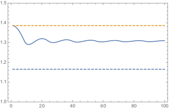
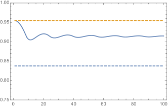
Figure 5: (Left) $C_{E}(\{{\cal N}_{\eta_{k}}\},n,\epsilon)$ vs $n$ for $\Delta=5$ (solid line). The bottom (resp. top) dashed line represents the capacity $g(N)+g(\underline{\eta}N)-g((1-\underline{\eta})N)$ (resp. $g(N)+g((\underline{\eta}+\overline{\eta})N)-g((1-(\underline{\eta}+\overline{\eta}))N)$). (Right) $C_{E}(\{{\cal N}_{\eta_{k}}\},n,\epsilon)$ vs $n$ for $\Delta=5$ (solid line). The bottom (resp. top) dashed line represents the capacity $g(\underline{\eta}N)$ (resp. $g((\underline{\eta}+\overline{\eta})N)$). The values of other parameters are $\underline{\eta}=0.4,\overline{\eta}=0.1,N=1$.

As for what concerns the variance of $\overline{C_{E}}(\{{\cal N}_{\eta_{k}}\},n)$ and of $\overline{C}(\{{\cal N}_{\eta_{k}}\},n)$, the behavior is quite similar to that of Fig.3.

7 Conclusion

In conclusion, we studied quantum channels that vary from one to another use in a deterministic way. To analyze their ability in transmitting classical information we resorted to a smoothed version of quantum relative entropy. As the first result, we derived a generalization of the relation between smooth and standard quantum relative entropies to the case of tensor product of non-identical density operators, which is valid also for separable Hilbert spaces (Eq.(2.9)). We then proved coding theorems for the classical entanglement assisted and unassisted capacities (Theorems 1 and 5 respectively). For that, we used position-based coding and quantum union bound applied to sequential decoding. The results were then adapted, with the help of input energy constraints, to continuous variable quantum channels, specifically lossy bosonic. Finally, enlightening examples were put forward in this context. They show that only when the sequence of channels parameter has a well defined limit, the capacities can be easily evaluated. The approach taken allowed us to evaluate the maximum transmission rate for any number of channel uses and estimate the error.

The natural extension of this work would be the study of time-varying channels in a non-deterministic way. Quite generally channels that are selected over the uses according to a probability distribution that is itself varying from one to another use, thus generalizing the arbitrarily varying channel model. We are confident that the mathematical tools developed here will be useful to this end. In another direction, one can pursue the quantum capacity of the introduced sequences of channels, which however needs slightly different tools.

Appendix A Second-order asymptotic

In this Appendix we derive Eq.(2.9), which represents a generalization of the relation between smooth and standard quantum relative entropies to the case of tensor product of non identical density operators, which is valid also for separable Hilbert spaces. The proof of inequality $\geq$ in Eq.(2.9) is based on [23, 14, 16].

Let us assume $\rho_{i},\sigma_{i}$, for $i=1,2,\ldots$ be full rank density operators on Hilbert space $\mathcal{H}$. Let us consider their spectral decompositions as follows

$$\rho_{i}=\sum_{x_{i}}\lambda_{x_{i}}P_{x_{i}}\,,$$ (A.1)

and

$$\sigma_{i}=\sum_{y_{i}}\mu_{y_{i}}Q_{y_{i}}\,.$$ (A.2)

We also define two distributions for any two density operators $\rho=\sum_{x}\lambda_{x}P_{x}$ and $\sigma=\sum_{x}\mu_{x}Q_{y}$ as follows

$$P_{\rho,\sigma}=\lambda_{x}\operatorname{Tr}(P_{x}Q_{y})\,,$$ (A.3)

and

$$Q_{\rho,\sigma}=\mu_{y}\operatorname{Tr}(P_{x}Q_{y})\,.$$ (A.4)

We then introduce

$$P_{\rho,\sigma}^{n}(x_{1},\ldots,x_{n})=\prod_{i}P_{\rho,\sigma}(x_{i})\,,$$ (A.5)

and

$$Q_{\rho,\sigma}^{n}(x_{1},\ldots,x_{n})=\prod_{i}Q_{\rho,\sigma}(y_{i})\,.$$ (A.6)

Lemma 9

Let $\rho$ and $\sigma$ be two density operators acting on a separable Hilbert space $\mathcal{H}$. For a given number $L$, there exists a measurement operator $T_{L}$ ($0\leq T_{L}\leq I$ ) such that

$$\operatorname{Tr}(T_{L}\rho)\geq\operatorname{Pr}(Z\geq\log{L}),\quad\operatorname{Tr}(T_{L}\sigma)\leq\frac{1}{L}\,,$$ (A.7)

where $Z$ is a random variable defined by $Z\equiv\log P_{\rho,\sigma}(X)-\log Q_{\rho,\sigma}(X)$.

Let $\bar{Z}=\frac{1}{n}\sum_{i}Z_{i}$ be the average over $n$ independent but not identical random variables $Z_{i}=\log P_{\rho,\sigma}(X_{i})-\log Q_{\rho,\sigma}(X_{i})$. For each $i$, set

$$\mu_{i}\equiv D(P_{\rho_{i},\sigma_{i}}\|Q_{\rho_{i},\sigma_{i}})=D(\rho_{i}\|\sigma_{i}),\quad s_{i}^{2}\equiv V(P_{\rho_{i},\sigma_{i}}\|Q_{\rho_{i},\sigma_{i}})=V(\rho_{i}\|\sigma_{i}),$$ (A.8)

and

$$t_{n}\equiv\mathbb{E}\left((Z_{n}-\mu_{i})^{3}\right)=\mathbb{E}\left(|\log P_{i}(X_{i})-\log Q_{i}(X_{i})-D(P\|Q)|^{3}\right)\,.$$ (A.9)

Now, we use the following Theorem which is a generalization of the central limit Theorem for independent but not identical random variables.

Theorem 10

[27]. Let the $\{X_{n}\}$ be random variables such that

$$\mathbb{E}(X_{n})=0,\qquad\mathbb{E}(X_{n}^{2})=s_{n}^{2},\qquad\mathbb{E}(|X_{n}|^{3})=t_{n}\,,$$ (A.10)

Put

$$\tilde{s}_{n}^{2}=s_{1}^{2}+\cdots+s_{n}^{2},\qquad\tilde{t}_{n}=t_{1}+\cdots+t_{n}\,,$$ (A.11)

and denoted by $P^{n}$ the distribution of the normalized sum $(X_{1}+\cdots+X_{n})/\tilde{s}_{n}$, then under the following condition

$$\lim_{n\to\infty}\frac{6\tilde{t}_{n}}{\tilde{s}_{n}^{3}}=0\,,$$ (A.12)

for all $x$ and $n$, we have

$$\left|P^{n}\left(\frac{X_{1}+\cdots+X_{n}}{\tilde{s}_{n}}\leq x\right)-\Phi(x)\right|\leq\frac{6\tilde{t}_{n}}{\tilde{s}_{n}^{3}}\,,$$ (A.13)

where

$$\Phi(x)\equiv\int_{-\infty}^{x}\frac{1}{\sqrt{2\pi}}e^{-y^{2}/2}dy\,.$$ (A.14)

Proposition 11

Let $\rho_{1},\rho_{2},\cdots$ and $\sigma_{1},\sigma_{2},\cdots$ denote states acting on a separable Hilbert space $\mathcal{H}$. Suppose that $D(\rho_{i}\|\sigma_{i}),V(\rho_{i}\|\sigma_{i}),T(\rho_{i}\|\sigma_{i})<\infty$ and $V(\rho_{i}\|\sigma_{i})>0$, for each $i=1,2,3,\cdots$. Suppose $n$ is sufficiently large such that $\varepsilon-\frac{6\sum_{i=0}^{n}\left[T(\rho_{i}\|\sigma_{i})\right]}{\sqrt{\left[\sum_{i=0}^{n}V\left(\rho_{i}\|\sigma_{i})\right)\right]^{3}}}\geq 0$. Then

$$D_{H}^{\varepsilon}\left(\bigotimes_{i=1}^{n}\rho_{i}\Big{\|}\bigotimes_{i=1}^{n}\sigma_{i}\right) =\sum_{i=1}^{n}D(\rho_{i}\|\sigma_{i})+\sqrt{\sum_{i=1}^{n}V(\rho_{i}\|\sigma_{i})}\Phi^{-1}\!\left(\varepsilon-\frac{6\sum_{i=0}^{n}\left[T(\rho_{i}\|\sigma_{i})\right]}{\sqrt{\left[\sum_{i=0}^{n}V\left(\rho_{i}\|\sigma_{i})\right)\right]^{3}}}\right)$$ (A.15)

$$=\sum_{i=1}^{n}D(\rho_{i}\|\sigma_{i})+\sqrt{\sum_{i=1}^{n}V(\rho_{i}\|\sigma_{i})}\Phi^{-1}\!\left(\varepsilon\right)+O(\log n).$$ (A.16)

Proof. (Part $\geq$) Applying the Berry–Esseen theorem [27] to the random sequence $Z_{1}-D(\rho_{1}\|\sigma_{1})$, …, $Z_{n}-D(\rho_{n}\|\sigma_{n})$, we find that

$$\left|\Pr\left\{\frac{\overline{Z}^{n}}{\sqrt{\left[\sum_{i=0}^{n}V\left(\rho_{i}\|\sigma_{i})\right)\right]^{3}}}\leq x\right\}-\Phi(x)\right|\leq\alpha(n),$$ (A.17)

where $\overline{Z}^{n}\equiv\frac{1}{n}\sum_{i=1}^{n}\left[Z_{i}-D(\rho_{i}\|\sigma_{i})\right]$ and $\alpha(n)\equiv\frac{6\sum_{i=0}^{n}\left[T(\rho_{i}\|\sigma_{i})\right]}{\sqrt{\left[\sum_{i=0}^{n}V\left(\rho_{i}\|\sigma_{i})\right)\right]^{3}}}$, which implies that

$$\Pr\left\{\sum_{i=1}^{n}Z_{i}\leq\sum_{i=1}^{n}D(\rho_{i}\|\sigma_{i})+nx\sqrt{\left[\sum_{i=0}^{n}V\left(\rho_{i}\|\sigma_{i})\right)\right]^{3}}\right\}\leq\Phi(x)+\alpha(n).$$ (A.18)

Picking $x=\Phi^{-1}\!\left(\varepsilon-\frac{6\cdot\tilde{t}_{n}}{\tilde{s}_{n}^{3}}\right)$, this becomes

$$\Pr\left\{\sum_{i=1}^{n}Z_{i}\leq\sum_{i=1}^{n}D(\rho_{i}\|\sigma_{i})+\sqrt{\sum_{i=1}^{n}V(\rho_{i}\|\sigma_{i})}\Phi^{-1}\!\left(\varepsilon-\alpha(n)\right)\right\}\leq\varepsilon.$$ (A.19)

Choosing $L$ such that

$$\log L=\sum_{i=1}^{n}D(\rho_{i}\|\sigma_{i})+\sqrt{\sum_{i=1}^{n}V(\rho_{i}\|\sigma_{i})}\Phi^{-1}\!\left(\varepsilon-\alpha(n)\right),$$ (A.20)

and applying Lemma 9, we find that

$$\operatorname{Tr}\{T^{n}\bigotimes_{i=1}^{n}\rho_{i}\}\geq\Pr\left\{\sum_{i=1}^{n}Z_{i}\geq\log L\right\}=1-\Pr\left\{\sum_{i=1}^{n}Z_{i}\leq\log L\right\}\geq 1-\varepsilon,$$ (A.21)

while

$$\operatorname{Tr}\{T^{n}\bigotimes_{i=1}^{n}\sigma_{i}\}\leq\frac{1}{L}=\exp\left\{-\left[\sum_{i=1}^{n}D(\rho_{i}\|\sigma_{i})+\sqrt{\sum_{i=1}^{n}V(\rho_{i}\|\sigma_{i})}\Phi^{-1}\!\left(\varepsilon-\alpha(n)\right)\right]\right\}.$$ (A.22)

This implies that

$$-\log\operatorname{Tr}\left\{T^{n}\bigotimes_{i=1}^{n}\sigma_{i}\right\}\geq\sum_{i=1}^{n}D(\rho_{i}\|\sigma_{i})+\sqrt{\sum_{i=1}^{n}V(\rho_{i}\|\sigma_{i})}\Phi^{-1}\!\left(\varepsilon-\alpha(n)\right).$$ (A.23)

Since $D_{H}^{\varepsilon}(\bigotimes_{i=1}^{n}\rho_{i}\|\bigotimes_{i=1}^{n}\sigma_{i})$ involves an optimization over all possible measurement operators $T^{n}$ satisfying $\operatorname{Tr}\{T^{n}\bigotimes_{i=1}^{n}\rho_{i}\}\geq 1-\varepsilon$, we conclude that the bound $\geq$ in (A.15) holds true. The equality (A.16) follows from expanding $\Phi^{-1}$ at the point $\varepsilon$ using Lagrange’s mean value theorem.

(Part $\leq$) We use the following

Theorem 12

[8] Let $\rho$ and $\sigma$ be density operators acting on a separable Hilbert space $\mathcal{H}$, let $T$ be a measurement operator acting on $\mathcal{H}$ and such that $0\leq T\leq I$, and let $\nu,\theta\in\mathds{R}$. Then

$$e^{-\theta}\operatorname{Tr}\{(I-T)\rho+\operatorname{Tr}\{T\sigma\}\geq\frac{e^{-\eta}}{1+e^{\nu-\theta}}\operatorname{Pr}\{X\leq\nu\}\,,$$ (A.24)

where $X$ is a random variable taking values $\log(\lambda_{x}/\mu_{y})$ with probability $\lambda_{x}\operatorname{Tr}(P_{x}Q_{y})$.

Then, the proof closely follows the proof of Proposition $2$ in  [13], which is based on  [23]. Choosing

$$\nu_{n}=\sum_{i=1}^{n}D(\rho_{i}\|\sigma_{i})+\sqrt{\sum_{i=1}^{n}V(\rho_{i}\|\sigma_{i})}\Phi^{-1}\!\left(\varepsilon+\frac{2}{\sqrt{n}}+\alpha(n)\right)\,,$$ (A.25)

and $\theta_{n}=\nu_{n}+\frac{1}{2}\log n$, we get

$$\operatorname{Tr}\{T^{n}\otimes_{i=1}^{n}\sigma_{i}\}\geq\left\{e^{-\sum_{i=1}^{n}D(\rho_{i}\|\sigma_{i})-\sqrt{\sum_{i=1}^{n}V(\rho_{i}\|\sigma_{i})}\Phi^{-1}(\varepsilon+2n^{-1/2}+\alpha(n))-\frac{1}{2}\log{n}}\right\}\left(\frac{1}{1+n^{-1/2}}\right)\,,$$ (A.26)

where $\operatorname{Tr}\left\{(I^{\otimes n}-T^{n})\otimes_{i=1}^{n}\rho_{i}\right\}\leq\varepsilon$. In this way we find

$$-\log{\operatorname{Tr}\{T^{n}\otimes_{i=1}^{n}\sigma_{i}\}}\leq\sum_{i=1}^{n}D(\rho_{i}\|\sigma_{i})+\sqrt{\sum_{i=1}^{n}V(\rho_{i}\|\sigma_{i})}\Phi^{-1}(\varepsilon+2n^{-1/2}+\alpha(n))+\frac{1}{2}\log{n}-\log{\frac{1}{1+n^{-1/2}}}\,.$$ (A.27)

References

- [1] M. M. Wilde. Quantum Information Theory. Cambridge University Press, Cambridge (2013).
- [2] F. Caruso, V. Giovannetti, C. Lupo, and S. Mancini. Quantum channels and memory effects. Reviews of Modern Physics. 86(4), 1203–1259, (2014).
- [3] I. Bjelakovic, H. Boche, and J. Nötzel. Quantum capacity of a class of compound channels. Physical Review A 78(4), 042331 (2008).
- [4] R. Ahlswede and V. Blinovsky. Classical capacity of classical quantum arbitrarily varying channels. IEEE Transactions on Information Theory, 53(2), 526-533, (2007).
- [5] H. Boche, C. Deppe, J. Nötzel, and A. Winter. Fully Quantum Arbitrarily Varying Channels: Random Coding Capacity and Capacity Dichotomy. IEEE International Symposium on Information Theory (ISIT), Vail, CO, 2018, pp. 2012-2016, (2018).
- [6] H. Boche, G. Jansen, and S. Kaltenstadler. Entanglement-assisted classical capacities of compound and arbitrarily varying quantum channels. Quantum Information Processing, 16, 88 (2017).
- [7] R. Ahlswede, I. Bjelakovic, H. Boche, J. Nötzel . Quantum capacity under adversarial noise: arbitrarily varying quantum channels. Communications in Mathematical Physics, 317, 103-156 (2013).
- [8] V. Jaksic, Y. Ogata, C.A. Pillet, and R. Seiringer. Quantum hypothesis testing and non-equilibrium statistical mechanics. Review of Mathematical Physics, 24(06), 1230002 (2012).
- [9] H. Qi, Q. Wang, and M. M. Wilde. Applications of position-based coding to classical communication over quantum channels. Journal of Physics A, 51(44), 444002, (2018).
- [10] A. Anshu, R. Jain, and N. A. Warsi. One shot entanglement assisted classical and quantum communication over noisy quantum channels: A hypothesis testing and convex split approach. arXiv:1702.01940.
- [11] M. M. Wilde. Sequential decoding of a general classical-quantum channel. Proceedings of the Royal Society of London A: Mathematical, Physical and Engineering Sciences, 469, 2157, (2013).
- [12] F. Buscemi and N. Datta. The Quantum Capacity of Channels With Arbitrarily Correlated Noise. IEEE Transactions on Information Theory 56(3), 1447-1460 (2010).
- [13] E. Kaur, and M. M. Wilde. Upper bounds on secret-key agreement over lossy thermal bosonic channels. Physical Review A, 96(6), 062318 (2017).
- [14] K. Li. Second-order asymptotics for quantum hypothesis testing. Annals of Statistics, 42(1), 171–189, (2014).
- [15] M. Tomamichel and M. Hayashi. A Hierarchy of Information Quantities for Finite Block Length Analysis of Quantum Tasks. IEEE Transactions on Information Theory, 59(11), 7693-7710, (2013).
- [16] S. Khabbazi-Oskouei, S. Mancini, and M. M. Wilde. Union bound for quantum information processing. Proceedings of the Royal Society A: Mathematical, Physical and Engineering Sciences, 475(2221), 20180612 (2019).
- [17] G. Matz, and F. Hlawatsch. Fundamentals of Time-Varying Communication Channels. Wireless Communications Over Rapidly Time-Varying Channels, Editors F. Hlawatsch and G. Matz. Academic Press, Oxford, 1-63 (2011).
- [18] W. E. Ryan and Li Han. Modulation and coding for short-duration deterministically time-varying channels. Proceedings IEEE International Conference on Communications ICC 1995, Volume 3, 1790-1794 (1995).
- [19] L. Wang, and R. Renner. One-Shot Classical-Quantum Capacity and Hypothesis Testing. Physical Review Letters, 108(20), 200501 (2012).
- [20] N. Datta, and M. Hsieh. One-shot entanglement-assisted quantum and classical communication. IEEE Transactions on Information Theory, 59(3), 1929-1939 (2013).
- [21] W. Matthews and S. Wehner. Finite block length converse bounds for quantum channels. IEEE Transactions on Information Theory, 60(11), 7317-7329 (2014).
- [22] G. Lindblad. Entropy, information and quantum measurements. Communication in Mathematical Physics, 33(24), 305-322, (1973).
- [23] N. Datta, Y. Pautrat, and C. Rouzè. Second-order asymptotics for quantum hypothesis testing in settings beyond i.i.d. quantum lattice systems and more. Journal of Mathematical Physics, 57(6), 062207 (2016).
- [24] M. M. Wilde. Position-based coding and convex splitting for private communication over quantum channels. Quantum Information Processing, 16(10) 264 (2017).
- [25] A. S. Holevo, M. Sohma, and O. Hirota. Capacity of quantum Gaussian channels. Physical Review A, 59(3), 1820–1828 (1999).
- [26] M. M. Wilde, J. M. Renes, and S. Guha. Second-order coding rates for pure-loss bosonic channels. Quantum Information Processing, 15, 1289–1308, (2016).
- [27] W. Feller. An Introduction to Probability Theory and Its Applications. John Wiley and Sons (1991).