Holographic Schwinger effect in the confining background with D-instanton

Abstract

Using the gauge-gravity duality, we study the holographic Schwinger effect by performing the potential analysis on the confining D3- and D4-brane background with D-instantons then evaluate the pair production/decay rate by taking account into a fundamental string and a single flavor brane respectively. The two confining backgrounds with D-instantons are obtained from the black D(-1)-D3 and D0-D4 solution with a double Wick rotation. The total potential and pair production/decay rate in the Schwinger effect are calculated numerically by examining the NG action of a fundamental string and the DBI action of a single flavor brane all in the presence of an electric field. In both backgrounds our numerical calculation agrees with the critical electric field evaluated from the DBI action and shows the potential barrier is increased by the presence of the D-instantons, thus the production/decay rate is suppressed by the D-instantons. Our interpretation is that particles in the dual field theory could acquire an effective mass through the Chern-Simons interaction or the theta term due to the presence of D-instantons so that the pair production/decay rate in Schwinger effect is suppressed since it behaves as $e^{-m^{2}}$. Our conclusion is in agreement with the previous results obtained in the deconfined D(-1)-D3 background at zero temperature limit and from the approach of the flavor brane in the D0-D4 background. In this sense, this work may be also remarkable to study the phase transition in Maxwell-Chern-Simons theory and observable effects by the theta angle in QCD.

1 Introduction

People have achieved many advances in the researches about the phenomena with strong electromagnetic field in the heavy-ion collision. The Schwinger effect as one of the most famous phenomenon attracts great interests since it is significantly related to the particle creation rate. Specifically the charged particles in the collisions at high speed can generate an extremely strong electromagnetic field so that the virtual pairs of particles in the vacuum can become real particles [1, 2]. Thus the Schwinger effect may be very helpful to study particle creation and thermalization in the heavy-ion collision. On the other hand, the P or CP violation in QCD (Quantum Chromodynamics) is also an important topic [3]. Usually a theta term can be added to the gauge theory to include the P or CP violation in the action,

$$S=-\frac{1}{2g_{YM}^{2}}\mathrm{Tr}\int F\wedge^{*}F+i\frac{\theta}{8\pi^{2}}\mathrm{Tr}\int F\wedge F,$$ (1.1)

where $g_{YM}$ refers to the Yang-Mills coupling constant. Although the experimental value of the theta angle is very small $\left(\left|\theta\right|\leq 10^{-10}\right)$, the theta-dependence in Yang-Mills theory or QCD is very interesting both in the theoretical and phenomenological researches, e.g. study of the phase transition of confinement/deconfinement [4, 5], the large $N$ behavior [6], the glueball spectrum [7] all in the presence of a theta angle. Particularly whether a theta vacua can be created in heavy-ion collision is still an open question which therefore attracts many investigations [8, 9, 10, 11] and moreover there have been some observable effects proposed in order to confirm the theta-dependence in the heavy-ion collision e.g. the chiral magnet effect [12, 13].

Accordingly the motivation of this work is to explore the Schwinger effect with the theta angle in the QCD-like or confining theory since the Schwinger effect would be affected by the theta angle and it might be remarkable to confirm the existence of the theta vacuum. However, using QFT (quantum field theory) frame work to analyze the Schwinger effect in a QCD-like or confining theory would be very challenging since the original Schwinger’s work shows that this effect must be non-perturbative. Fortunately, the gauge-gravity duality could provide an alternative way [14, 15] to analyze the Schwinger effect by evaluating the total potential in holography [16]. In order to study the QCD-like theory, the confining background geometry is also necessary. Taking account into the frame work of string theory, the most famous confining (soliton) background geometry is obtained by a double Wick rotation on the black D3- or D4-brane solution [17, 18], so the holographic total potential of Schwinger effect can be calculated by performing the potential analysis [19] in these backgrounds as in [20, 21]. To involve the theta angle or the topological charge in the dual field theory, we additionally need to introduce D-instantons into the D3- and D4-brane solution. This can be achieved by considering the black D(-1)-D3 [22, 23, 24, 25] and D0-D4 brane solution [26, 27] with a double Wick rotation, following the discussion in [17, 18]. Afterwards the D(-1) and D0-branes play the role of the D-instantons and holographically correspond to the coupling constant of the Chern-Simons term or the theta anglein the dual theory [27, 28, 29, 30, 31].

In this project, we will perform the potential analysis [19] for the holographic Schwinger effect in the soliton D3- and D4-brane background with D-instantons respectively, then evaluate the production/decay rate by involving a fundamental string and a single flavor brane. Our analysis shows the Schwinger effect occurs above a certain critical electric field. The presence of the D-instantons increases the critical electric field and the potential barrier of the Schwinger effect, thus suppresses the production/decay rate both in the D(-1)-D3 and D0-D4 background. The numerical calculation of the fundamental string and the flavor brane consistently supports our analysis which might imply the universal features of the Schwinger effect with instantons.

The outline of this paper is as follows. In Section 2, we give a brief construction for the confining D3- and D4-brane background with D-instantons. In Section 3, we perform potential analysis for the holographic Schwinger effect then calculate the total potential numerically. In Section 4, the pair production rate is evaluated with D-instantons. As a supplement to this work, we analyze parallelly the Schwinger effect by taking account into a single flavor in Section 5 and in Section 6, we give our summary and discussion of this work. Basically our work is an extension to [20, 21], also a different approach to check the results obtained in the deconfined D(-1)-D3 background at zero temperature limit [32] and the flavor brane setup for holographic Schwinger effect in [33].

2 The confining geometry with D-instanton

2.1 The confining D(-1)-D3 solution

The D(-1)-D3 brane system was proposed in [22] which is represented by a deformed D3-brane solution with a Ramond-Ramond (RR) nontrivial scalar field. And the Ramond-Ramond (RR) scalar charge is balanced by the dilaton in order to preserve 1/2 of supersymmetry. This system is recognized as a marginal “bound state” of D3-branes with smeared D(-1)-branes , i.e. the D-instantons and its low-energy dynamics is described by the type IIB supergravity action. The non-extremal solution for the black D3-branes with D(-1)-branes as D-instantons can be found in [23]. However, in this section we will focus on the confinement construction of this solution.

The most simple way to obtain a confinement theory is to follow the discussion in [17, 18]. Specifically the first step is to take one of the three spatial dimensions $x^{i}$ to be compactified on a circle with period $x^{i}\sim x^{i}+\delta x^{i}$. So the dual theory ($\mathcal{N}=4$ Super Yang-Mills theory) becomes effectively 3-dimensional (3d) below the Kaluza-Klein energy scale $M_{KK}=1/\delta x^{i}$. Then the second step is to get rid of all massless particles other than the gauge fields. The most convenient way to achieve this is to require the fermion fields to be anti-periodic on the circle while the bosons are given periodic boundary conditions. Hence the supersymmetric fermions acquire mass of order $M_{KK}$ and the scalars of the SYM theory also get masses of order $M_{KK}$ induced by radiative corrections. Therefore the supersymmetry and conformal symmetry are broken down and the resultant theory would be three-dimensional YM theory below the energy scale $M_{KK}$. Next we have to identify the bulk supergravity geometry as its holographic correspondence. A trick for obtaining the answer is to perform a double Wick rotation on the D(-1)-D3 brane background i.e. $t\rightarrow-ix^{i},x^{i}\rightarrow-it$. Without loss of generality, let us denote $x^{i}=x^{3}$, then the confining solution for D3-branes with smeared D-instantons reads,

$$ds^{2} =e^{\phi/2}\left\{\frac{r^{2}}{R^{2}}\left[-dt^{2}+\left(dx^{1}\right)^{2}+\left(dx^{2}\right)^{2}+f\left(r\right)\left(dx^{3}\right)^{2}\right]+\frac{1}{f\left(r\right)}\frac{R^{2}}{r^{2}}dr^{2}+R^{2}d\Omega_{5}^{2}\right\},$$

$$e^{\phi} =1+\frac{Q}{r_{KK}^{4}}\log\frac{1}{f\left(r\right)},\ C=-e^{-\phi}+C_{0},\ f\left(r\right)=1-\frac{r_{KK}^{4}}{r^{4}},\ F_{5}=\mathcal{Q}_{3}\epsilon_{5}$$ (2.1)

where $C$ is the RR 0-form with $F_{1}=dC$, $R^{4}=4\pi g_{s}l_{s}^{4}$ and $Q,\mathcal{Q}_{3}$ relates to the charge of the D-instantons and D3-branes. $\epsilon_{5}$ represents the volume form of a unit $S^{5}$. The above solution is defined for $r>r_{KK}$ only thus it does not have a horizon. This means $r=r_{KK}$ is the end of the spacetime. Since the warp factor $e^{\phi/2}\frac{r^{2}}{R^{2}}$ never goes to zero, the asymptotics of the Wilson loop in this geometry would lead to an area law which implies the holographically dual field theory exhibits confinement below $M_{KK}$.  In order to avoid conical singularities in the dual field theory, the following constraint has to be additionally required,

$$M_{KK}=\frac{2r_{KK}}{R^{2}}.$$ (2.2)

We note that if $Q\rightarrow 0$ (i.e. no D-instantons) the supergravity solution (2.1) consistently returns to the confining D3-brane solution which is used in [18, 20, 21]. The dual field theory can be examined by considering a probe D3-brane located at $r\rightarrow\infty$ whose action is

$$S_{\mathrm{D}3} =\left[-T_{\mathrm{D}3}\int d^{4}xe^{-\frac{\phi}{2}}\mathrm{Str}\sqrt{-\det\left(g+\mathcal{F}\right)}+T_{\mathrm{D}3}\int C_{4}+\frac{1}{2}T_{\mathrm{D}3}\mathrm{Tr}\int C_{0}\mathcal{F}\land\mathcal{F}\right]\bigg{|}_{r\rightarrow\infty}$$

$$\simeq-\frac{1}{4g_{4,YM}^{2}}\int d^{4}xF_{\mu\nu}F^{\mu\nu}+\frac{\kappa}{2}\mathrm{Tr}\int F\wedge F+\mathcal{O}\left(F^{3}\right)$$

$$=-\frac{1}{4g_{3,YM}^{2}}\int d^{3}xF_{ab}F^{ab}+\frac{\kappa}{2}\mathrm{Tr}\int\omega_{3}.$$ (2.3)

Here$\mathcal{F}=2\pi\alpha^{\prime}F$ denotes the gauge field strength and $T_{\mathrm{D3}}$ denotes the tension of D3-brane. $g_{4,3,YM}$ refers to the 4d and 3d Yang-Mills coupling constant respectively and $\omega_{3}$ is the Chern-Simons (CS) 3-form. $\kappa$ corresponds to the boundary value of $C$. Accordingly, we can conclude the dual field theory to the background (2.1) is 3d confined YM plus CS theory below $M_{KK}$ in holography.

2.2 The confining D0-D4 solution

Basically the confining D0-D4 solution where the D0-brane plays the role of D-instanton can be achieved by following the same discussion in the last section. Its confining solution reads [27, 28],

$$ds^{2} =\left(\frac{r}{R}\right)^{3/2}\left[H_{0}^{1/2}\eta_{\mu\nu}dx^{\mu}dx^{\nu}+H_{0}^{-1/2}f\left(r\right)\left(dx^{4}\right)^{2}\right]+H_{0}^{1/2}\left(\frac{R}{r}\right)^{3/2}\left[\frac{1}{f\left(r\right)}dr^{2}+r^{2}d\Omega_{4}^{2}\right],$$

$$e^{\phi} =\left(\frac{r}{R}\right)^{3/4}H_{0}^{3/4},\ f\left(r\right)=1-\frac{r_{KK}^{3}}{r^{3}},\ H_{0}=1+\frac{Q}{r^{3}},$$

$$F_{2} =dC_{1}=\frac{\mathcal{Q}_{0}}{r^{4}}\frac{1}{H_{0}^{2}}dr\wedge dx^{4},\ F_{4}=dC_{3}=\mathcal{Q}_{4}\epsilon_{4},$$ (2.4)

where $Q,\mathcal{Q}_{0}$ are two constants related to the number density of D0-branes and $\mathcal{Q}_{4}$ is the charge of D4-branes. We note that the D0-brane is the D-instanton in this system which extends along the direction $x^{4}$ and $x^{4}$ is periodic $x^{4}\sim x^{4}+\delta x^{4}$. To avoid conical singularities in the dual field theory, it leads to the constraint

$$M_{KK}=\frac{3}{2}\frac{r_{KK}^{1/2}}{R^{3/2}}\frac{1}{\sqrt{1+Q/r_{KK}^{3}}}.$$ (2.5)

Below $M_{KK}$ the dual field theory is confined theory which can be investigated by introducing a probe D4-brane in the background (2.4) at $r\rightarrow\infty$. Then its low-energy action is

$$S_{\mathrm{D}4} =\left[-T_{\mathrm{D}4}\int d^{5}xe^{-\phi}\mathrm{Str}\sqrt{-\det\left(g+\mathcal{F}\right)}+T_{4}\int C_{5}+\frac{1}{2}T_{\mathrm{D}4}\mathrm{Tr}\int C_{1}\land\mathcal{F}\land\mathcal{F}\right]\bigg{|}_{r\rightarrow\infty}$$

$$\simeq-\frac{1}{4g_{4,YM}^{2}}\int d^{4}xF_{\mu\nu}F^{\mu\nu}+\frac{\theta}{16\pi^{2}}\mathrm{Tr}\int F\wedge F+\mathcal{O}\left(F^{3}\right).$$ (2.6)

We note that the theta angle corresponds to $\theta\sim\int_{S_{x^{4}}}C_{1}$. Therefore the dual theory in the D0-D4 system is theta-dependent confined Yang-Mills theory [27, 29, 30].

3 Potential analysis

In this section, let us perform the analysis by following [19, 20, 21] for the confining background with D-instantons to evaluate the effective potential in Schwinger effect.

3.1 The D(-1)-D3 background

In order to study the Schwinger effect, we need to evaluate the effective potential and find the critical value of the electric field first. So let us start with a probe D3-brane located at $r=r_{0}$ on which an external electric field $F_{01}=E$ is switched. The DBI (Dirac-Born-Infeld) action of the probe brane is given as,

$$S =-T_{\mathrm{D}3}\int d^{4}xe^{-\frac{\phi}{2}}\sqrt{-\det\left(g+\mathcal{F}\right)}$$

$$=-T_{\mathrm{D}3}V_{4}\frac{r_{0}^{4}}{R^{4}}e^{\frac{\phi\left(r_{0}\right)}{2}}f\left(r_{0}\right)^{1/2}\sqrt{1-\frac{\left(2\pi\alpha^{\prime}\right)^{2}R^{4}}{e^{\phi\left(r_{0}\right)}r_{0}^{4}}E^{2}}.$$ (3.1)

It is easy to understand that the classical solution would not exist if $E>E_{c}$ where $E_{c}$ is a critical value of the electric field. Thus the critical electric field can be obtained as,

$$E_{c}=\frac{1}{2\pi\alpha^{\prime}}\frac{r_{0}^{2}}{R^{2}}e^{\frac{\phi\left(r_{0}\right)}{2}}.$$ (3.2)

Then we need to calculate the total energy of a pair of the fundamental particles which can be computed by evaluating the expectation of its rectangular Wilson loop. In holography it corresponds to the world-sheet area or equivalently the on-shell Nambu-Goto (NG) action of a fundamental string [34]. Accordingly we consider a Fermion-anti Fermion pair placed at fixed positions on the probe brane with separation $x$ in direction $x^{1}$. Choosing the static gauge, the induced metric on the world sheet with $\tau=t,x^{1}=\sigma,r=r\left(\sigma\right)$ is,

$$ds^{2}=g_{\alpha\beta}dx^{\alpha}dx^{\beta}=\frac{r^{2}}{R^{2}}e^{\phi/2}\left\{d\tau^{2}+\left[1+\frac{1}{f\left(r\right)}\frac{R^{4}}{r^{4}}\left(\frac{dr}{d\sigma}\right)^{2}\right]\left(d\sigma\right)^{2}\right\},\ \ \ \ \alpha,\beta=0,1$$ (3.3)

where we have worked in the Euclidean signature. Therefore the NG action is calculated as,

$$S_{NG} =T_{f}\int d\tau d\sigma\sqrt{\det\left(g_{\alpha\beta}\right)}$$

$$=T_{f}\int d\tau d\sigma\sqrt{e^{\phi\left(r\right)}\left[\frac{1}{f\left(r\right)}\left(\frac{dr}{d\sigma}\right)^{2}+\frac{r^{4}}{R^{4}}\right]}.$$ (3.4)

Since the Lagrangian in (3.4) does not depend on $\sigma$ explicitly, its associated Hamiltonian is conserved i.e. a constant,

$$\mathcal{H}=\left(\partial_{\sigma}r\right)\frac{\partial\mathcal{L}}{\partial_{\sigma}r}-\mathcal{L}=const,$$ (3.5)

which means

$$\frac{e^{\frac{\phi\left(r\right)}{2}}r^{4}/R^{4}}{\sqrt{\frac{r^{4}}{R^{4}}+\frac{1}{f\left(r\right)}\left(\frac{dr}{d\sigma}\right)^{2}}}=const.=e^{\frac{\phi\left(r_{c}\right)}{2}}\frac{r_{c}^{2}}{R^{2}},$$ (3.6)

if the boundary condition

$$\frac{dr}{d\sigma}\bigg{|}_{r=r_{c}}=0,\ \sigma=\sigma_{0}$$ (3.7)

is imposed where $r_{c}$ refers to the top point of the string in the bulk as illustrated in Figure 1.

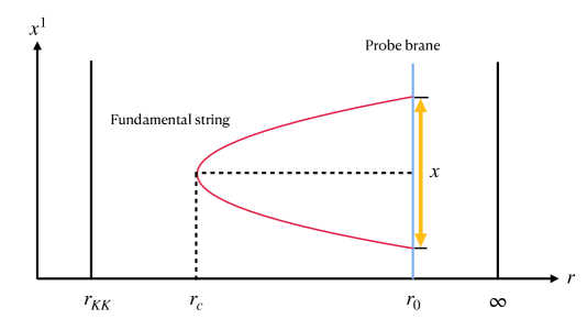
Figure 1: Configuration of the string and probe brane.

So (3.6) leads to

$$\frac{dr}{d\sigma}=\frac{1}{R^{2}}\sqrt{\left[e^{\phi\left(r\right)-\phi\left(r_{c}\right)}\frac{r^{4}}{r_{c}^{4}}-1\right]\left(r^{4}-r_{KK}^{4}\right)},$$ (3.8)

and the separation $x$ is therefore obtained as

$$x=\frac{2R^{2}}{r_{0}a}e^{\phi\left(1\right)/2}\int_{1}^{1/a}\frac{dy}{\sqrt{\left(y^{4}-b^{4}/a^{4}\right)\left[e^{\phi\left(y\right)-\phi\left(1\right)}y^{4}-1\right]}},$$ (3.9)

where we have used the dimensionless quantities defined as,

$$y=\frac{r}{r_{c}},\ a=\frac{r_{c}}{r_{0}},\ b=\frac{r_{KK}}{r_{0}},\ \frac{Q}{r_{0}^{4}}=q.$$ (3.10)

Afterwards the potential energy (PE) including static energy (SE) is computed as

$$V_{\mathrm{PE+SE}}=2T_{f}\int_{0}^{x/2}d\sigma\mathcal{L}=2T_{f}r_{0}a\int_{1}^{1/a}\frac{e^{\phi\left(y\right)}y^{4}}{\sqrt{\left(y^{4}-b^{4}/a^{4}\right)\left[e^{\phi\left(y\right)-\phi\left(1\right)}y^{4}-1\right]}}.$$ (3.11)

However we have to add the contribution from the interaction of the Fermion-anti Fermion pair with an external electric field $E$ to this energy. So the total potential is,

$$V_{\mathrm{tot}}\left(x\right) =V_{\mathrm{PE+SE}}-Ex$$

$$=2T_{f}r_{0}a\int_{1}^{1/a}\frac{e^{\phi\left(y\right)}y^{4}}{\sqrt{\left(y^{4}-b^{4}/a^{4}\right)\left[e^{\phi\left(y\right)-\phi\left(1\right)}y^{4}-1\right]}}$$

$$-\frac{2T_{f}r_{0}\alpha}{a}e^{\phi\left(1\right)}\int_{1}^{1/a}\frac{dy}{\sqrt{\left(y^{4}-b^{4}/a^{4}\right)\left[e^{\phi\left(y\right)-\phi\left(1\right)}y^{4}-1\right]}},$$ (3.12)

where

$$\alpha=\frac{E}{E_{c}\left(q\right)},\ E_{c}\left(q\right)=T_{f}\frac{r_{0}^{2}}{R^{2}}e^{\phi\left(1\right)/2},$$ (3.13)

and $E_{c}$ is the critical electric field given in (3.2). The relation of $V_{tot}$ and $x$ can be evaluated numerically which has been illustrated as in Figure 2 with various $q,\alpha$.

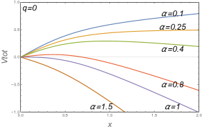
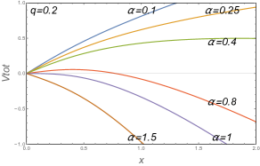
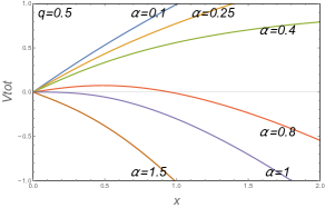
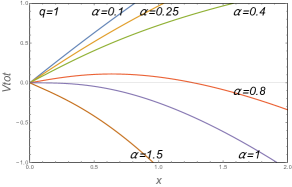
Figure 2: The dependence on $x$ of the total potential $V_{tot}\left(x\right)$ with various instanton densities and electric fields (determined by $\alpha$) in the confining D(-1)-D3 background. In all graphs we have set $b=0.5$ and $2L^{2}/r_{0}=2T_{f}r_{0}=1$.

In Figure 2 we have set $b=0.5$ (fixing energy scale $M_{KK}$) , $\alpha=0.4,0.6,0.8,1,1.2$ and the instanton density has been chosen as $q=0,0.2,0.5,1$ respectively in the four panels for comparison. These graphs imply that the potential barrier vanishes for $\alpha>1$, so the critical electric field obtained from the potential analysis agrees with (3.2) which is evaluated by using the DBI action as expected in [20, 35]. Besides we notice that the presence of instantons increases the potential barrier and thus suppresses the pair creation. This conclusion would be further confirmed by analyzing the formula (3.4) of the NG action and the expectation of a circular Wilson loop in the following sections. Nonetheless, to see this quickly, let us introduce another dimensionless parameter $\tilde{\alpha}=\frac{E}{E_{c}\left(q=0\right)}$ so that $E=E_{c}\left(q=0\right)$ corresponds to $\tilde{\alpha}=1$, then the numerical result of $V_{tot}\left(x\right)$ and $q$ is shown in Figure 3.

Figure 3: The relation of $V_{tot}\left(x\right)$ and $q$ in the D(-1)-D3 background with $b=0.5,\tilde{\alpha}=1$.

We find there is not any limitation to pair creation at zero instanton density since there is no potential barrier in the presence of electric field for $q=0$. As we can see the presence of the instantons develops a potential barrier, so the Schwinger effect occurs through a tunneling process only if $q>0$ and the instanton density increases the potential barrier whereas suppresses the pair creation. It therefore implies that the critical electric field is also increased by the instanton density which is in agreement with (3.2). And all these conclusions agree with the results evaluated in the deconfined D(-1)-D3 background at zero temperature limit in [32].

3.2 The D0-D4 background

In this section, let us turn to the D0-D4 case. The discussion would be basically parallel to those in Section 3.2. First we consider the DBI action of a probe D4-brane in the D0-D4 background with an electric field located at $r=r_{0}$. The action takes the form,

$$S =-T_{\mathrm{D4}}\int d^{5}xe^{-\phi}\sqrt{-\det\left(g+\mathcal{F}\right)}$$

$$=-T_{\mathrm{D4}}V_{5}\frac{r^{3}}{R^{3}}f\left(r_{0}\right)^{1/2}\sqrt{1-\frac{\left(2\pi\alpha^{\prime}\right)^{2}R^{3}}{H_{0}\left(r_{0}\right)r_{0}^{3}}E^{2}}.$$ (3.14)

Hence the critical electric field is evaluated as,

$$E_{c}=\frac{1}{2\pi\alpha^{\prime}}\frac{r_{0}^{3/2}}{R^{3/2}}H_{0}^{1/2}\left(r_{0}\right).$$ (3.15)

Then the Euclidean induced metric on the world sheet of a fundamental string with the choice of static gauge $\tau=t,x^{1}=\sigma,r=r\left(\sigma\right)$ is given as,

$$ds^{2}=\left(\frac{r}{R}\right)^{3/2}H_{0}^{1/2}\left\{d\tau^{2}+\left[1+\frac{1}{f\left(r\right)}\left(\frac{R}{r}\right)^{3}\left(\frac{dr}{d\sigma}\right)^{2}\right]d\sigma^{2}\right\}.$$ (3.16)

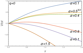
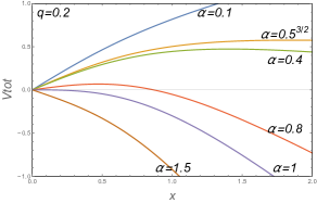
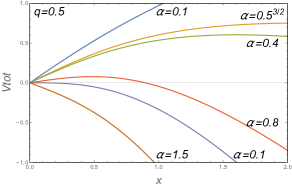
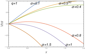
Figure 4: The dependence on $x$ of the total potential $V_{tot}\left(x\right)$ with various instanton densities and electric fields (determined by $\alpha$) in the confining D0-D4 background. In all graphs we have set $b=0.5$ and $2L^{3/2}/r_{0}^{1/2}=2T_{f}r_{0}=1$.

Therefore the NG action can be computed as,

$$S_{NG}=T_{f}\int d\tau d\sigma H_{0}^{1/2}\left(r\right)\sqrt{\frac{r^{3}}{R^{3}}+\frac{1}{f\left(r\right)}\left(\frac{dr}{d\sigma}\right)^{2}.}$$ (3.17)

The conserved Hamiltonian is

$$\frac{H_{0}^{1/2}\left(r\right)r^{3}/R^{3}}{\sqrt{\frac{r^{3}}{R^{3}}+\frac{1}{f\left(r\right)}\left(\frac{dr}{d\sigma}\right)^{2}}}=const.=\frac{r_{c}^{3/2}}{R^{3/2}}H_{0}^{1/2}\left(r_{c}\right),$$ (3.18)

where we have used the boundary condition

$$\frac{dr}{d\sigma}\bigg{|}_{r=r_{c}}=0,\ \sigma=\sigma_{0}.$$ (3.19)

So we have,

$$\frac{dr}{d\sigma}=\frac{1}{R^{3/2}H_{0}^{1/2}\left(r_{c}\right)}\sqrt{\left(r^{3}-r_{KK}^{3}\right)\left(\frac{r^{3}}{r_{c}^{3}}-1\right)},$$ (3.20)

which leads to the formula of the separation $x$ as,

$$x=2\int_{r_{c}}^{r_{0}}dr=\frac{2R^{3/2}}{r_{0}^{1/2}a^{1/2}}H_{0}^{1/2}\left(1\right)\int_{1}^{1/a}\frac{dy}{\sqrt{\left(y^{3}-1\right)\left(y^{3}-b^{3}/a^{3}\right)}},$$ (3.21)

with the dimensionless quantities introduced as,

$$y=\frac{r}{r_{c}},\ a=\frac{r_{c}}{r_{0}},\ b=\frac{r_{KK}}{r_{0}},\ \frac{Q}{r_{0}^{3}}=q.$$ (3.22)

Afterwards the potential energy (PE) including static energy (SE) in D0-D4 background is computed as,

$$V_{\mathrm{PE+SE}}=2T_{f}\int_{0}^{x/2}d\sigma\mathcal{L}=2T_{f}r_{0}a\int_{1}^{1/a}dy\frac{y^{3}H_{0}\left(y\right)}{\sqrt{\left(y^{3}-1\right)\left(y^{3}-b^{3}/a^{3}\right)}}.$$ (3.23)

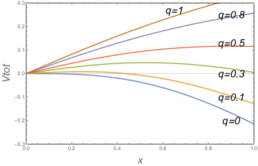
Figure 5: The relation of $V_{tot}\left(x\right)$ and $q$ in the D(-1)-D3 background with $b=0.5^{3/2},\tilde{\alpha}=1$.

By taking into account the contribution of the electric field, the total potential can be obtained as,

$$V_{\mathrm{tot}} =V_{\mathrm{PE+SE}}-Ex$$

$$=2T_{f}r_{0}a\int_{1}^{1/a}dy\frac{y^{3}H_{0}\left(y\right)}{\sqrt{\left(y^{3}-1\right)\left(y^{3}-b^{3}/a^{3}\right)}}-\frac{2T_{f}r_{0}\alpha}{a^{1/2}}H_{0}\left(1\right)\int_{1}^{1/a}\frac{dy}{\sqrt{\left(y^{3}-1\right)\left(y^{3}-b^{3}/a^{3}\right)}},$$ (3.24)

where

$$\alpha=\frac{E}{E_{c}},\ E_{c}=\frac{1}{2\pi\alpha^{\prime}}\frac{r_{0}^{3/2}}{R^{3/2}}H_{0}^{1/2}\left(r_{0}\right).$$ (3.25)

The relation of $V_{tot}$ and $x$ in the D4-D0 background can be evaluated numerically and the results are illustrated as in Figure 4. These graphs also show that the potential barrier vanishes for $\alpha>1$ which agrees with our (3.15) and again the potential analysis as expected in [20, 35]. By introducing $\tilde{\alpha}=\frac{E}{E_{c}\left(q=0\right)}$, we find the presence of the instantons develops a potential barrier and increases it as illustrated in Figure 5. So the Schwinger effect can occur without any any limitation at $q=0$ while it happens only through a tunneling process for $q>0$. Since the instantons increase the potential barrier, it suppresses the pair creation. And this conclusion is in agreement with the analysis from the flavor brane approach for the Schwinger effect in the D0-D4 background in [33].

4 Pair production rate

To exactly analyze the Schwinger effect, we are going to compute the pair production rate in this section. As mentioned before, this quantity can be obtained by evaluating the expectation of a circular Wilson loop living in the $t-x$ plane in the presence of an external electric field. Following the discussion in [21], the expectation of the Wilson loop corresponds to the Euclidean version of the string onshenll action in holography. So let us work in the Euclidean signature and choose the polar coordinates in the $t-x$ plane as,

$$t=\rho\cos\eta,\sigma=\rho\sin\eta,$$ (4.1)

with all constant other coordinates. Since the D(-1)-D3 and D0-D4 background are the concerns, we will analyze the string action respectively in the two backgrounds.

The D(-1)-D3 case

Using (3.4) and (4.1), the string action can be written as,

$$S=S_{NG}+S_{B_{2}},$$ (4.2)

where

$$S_{NG} =2\pi T_{f}R^{2}\int d\rho e^{\phi/2}\frac{\rho}{z^{2}}\sqrt{1+\frac{z^{\prime 2}}{f}},\ f=1-\frac{z^{4}}{z_{KK}^{4}},$$

$$S_{B_{2}} =-2\pi T_{f}B_{01}\int_{0}^{x}d\rho\rho=-\pi Ex^{2}.$$ (4.3)

Here we have defined the $z$ coordinate as $z\left(\rho\right)=R^{2}/r$ and the derivatives are with respect to $\rho$. Therefore the classical equation of motion can be obtained by varying action (4.3) which is,

$$z^{\prime}+\frac{2\rho f\left(z\right)}{z}+\rho z^{\prime\prime}-\frac{\rho z^{\prime 2}}{2f\left(z\right)}\frac{d}{dz}f\left(z\right)+\frac{2\rho z^{\prime 2}}{z}+\frac{z^{\prime 3}}{f\left(z\right)}-\frac{1}{2}\rho\left[f\left(z\right)+z^{\prime 2}\right]\frac{d}{dz}\phi\left(z\right)=0.$$ (4.4)

In order to obtain the onshell action, we need to solve the above differential equation numerically which would however be very difficult. Fortunately this step can be a little simplified by imposing an additional constraint as pointed out in [21] which in our setup is,

$$z^{\prime}\left(\rho\right)\big{|}_{\rho=x}=-\sqrt{f\left(z\right)\left(\frac{e^{\phi}}{\alpha^{2}}-1\right)}\bigg{|}_{z=z_{0}}.$$ (4.5)

Altogether, we solve (4.4) numerically with the boundary condition $z^{\prime}\left(0\right)=0,z\left(0\right)=z_{c}$ and the constraint (4.5). Then the numerical result for the onshell action $S$ as a function of $\alpha$ and $q$ is illustrated in Figure 6

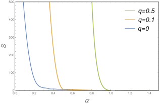
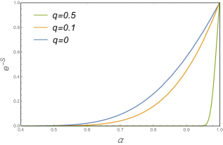
Figure 6: The classical string action and its exponential behavior versus $\alpha$ in the D(-1)-D3 background.

where its exponential behavior $e^{-S}$ is also plotted. The numerical calculation shows the pair production rate is indeed suppressed by the presence of the D-instantons which agrees with the potential analysis. And the the exponential behavior of the classical action approaches to zero $E_{c}$ obtained by the potential analysis.

The D0-D4 case

Let us evaluate the pair production rate in the D0-D4 background. Following the similar steps as the D(-1)-D3 case, the string action in the D0-D4 background reads,

$$S =S_{NG}+S_{B_{2}},$$

$$S_{NG} =16\pi T_{f}R^{3}\int d\rho\frac{H_{0}^{1/2}\left(z\right)\rho}{z^{3}}\sqrt{1+\frac{z^{\prime 2}}{f\left(z\right)}},\ f\left(z\right)=1-\frac{z^{6}}{z_{KK}^{6}},$$

$$S_{B_{2}} =-2\pi T_{f}B_{01}\int_{0}^{x}d\rho\rho=-\pi Ex^{2},$$ (4.6)

where we have imposed the following coordinate transformation,

$$z\left(\rho\right)=\frac{2R^{3/2}}{r^{1/2}}.$$ (4.7)

Varying action (4.6), the associated equation of motion is obtained as,

$$z^{\prime\prime}-\frac{f\left(z\right)+z^{\prime 2}}{2H_{0}\left(z\right)}\frac{d}{dz}H_{0}\left(z\right)+\frac{3f\left(z\right)+3z^{\prime 2}}{z}-\frac{z^{\prime 2}}{2f\left(z\right)}\frac{d}{dz}f\left(z\right)+\frac{z^{\prime 3}}{\rho f\left(z\right)}+\frac{z^{\prime}}{\rho}=0.$$ (4.8)

Again we solve the above differential equation with the boundary condition $z^{\prime}\left(0\right)=0,z\left(0\right)=z_{c}$ and an additional constraint,

$$z^{\prime}\left(\rho\right)\big{|}_{\rho=x}=-\sqrt{f\left(z\right)\left(\frac{H_{0}\left(z\right)}{\alpha^{2}}-1\right)}\bigg{|}_{z=z_{0}},$$ (4.9)

to obtain the onshell action. Afterwards the classical string action $S$ and its exponent are numerically evaluated in Figure 7

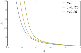
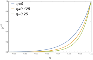
Figure 7: The classical string action and its exponential behavior versus $\alpha$ in the D0-D4 background.

. So we see again the pair production rate is suppressed by the presence of the D-instantons which is in agreement with the potential analysis in the D0-D4 background.

5 The electric instability with a single flavor

The analyse of the Schwinger effect in holography can also be extended by including flavor [33, 37, 38, 39], since it would also be significant to consider the vacuum instability and creation rate with the fundamental matters in the Schwinger effect, which can be introduced when the flavor brane is embedded into the background geometry. As a supplement to this project, in this section let us briefly take into account a single flavor brane and investigate the vacuum instability with an external electric field in the D(-1)-D3 and D0-D4 system respectively.

The D(-1)-D3 case

To involve the flavors in the dual theory, it is necessary to introduce the D7-branes as flavors as most approaches in the D3-brane system [40]. The configuration of various D-branes in the D(-1)-D3 system is given in Table 1.

	(-1)	0	1	2	3	4	5	6	7	8	9
D(-1)	-
D3-brane		-	-	-	-
D7-brane		-	-	-	-	-	-	-	-

Table 1: The configuration of the D-branes in the D(-1)-D3 system.

Without loss of generality, we can turn on the components $F_{01}=E,F_{0z},F_{1z}$ of the gauge field strength. Since the electric instability will be focused, we only need to consider a single D7-brane whose action is given as,

$$S_{\mathrm{D7}}=-T_{\mathrm{D7}}\int d^{8}xe^{-\phi}\sqrt{-\det\left(g_{\mathrm{D7}}+2\pi\alpha^{\prime}F\right)}-\mu_{7}\int C_{8}.$$ (5.1)

We note that the supersymmetry is broken down below the energy scale $M_{KK}$ in our setup. By imposing the background geometry (2.1) into (5.1), the action becomes,

$$S =-2\pi^{2}T_{\mathrm{D7}}V_{4}\int dze^{\phi}\frac{R^{8}}{z^{5}}\sqrt{\xi},$$

$$\xi =1-\left(2\pi\alpha^{\prime}\right)^{2}\frac{z^{4}}{R^{4}}e^{-\phi}\left[F_{01}^{2}+\left(F_{0z}^{2}-F_{1z}^{2}\right)f\left(z\right)\right],$$ (5.2)

which leads to the following equations of motion for the $U\left(1\right)$ gauge field strength,

$$\partial_{z}\left(\frac{f}{z\sqrt{\xi}}F_{0z}\right)=0, \partial_{0}\left(\frac{f}{z\sqrt{\xi}}F_{0z}\right)=0,$$

$$\partial_{0}\left(\frac{1}{z\sqrt{\xi}}F_{01}\right) +\partial_{z}\left[\frac{f}{z\sqrt{\xi}}F_{1z}\right]=0.$$ (5.3)

In particular, when the electric field is static i.e. time-independent, we can put $\partial_{0}=0$, the above equations of motion reduces to two constants $j,d$ as,

$$j\equiv 2\pi\alpha^{\prime}\frac{f}{z\sqrt{\xi}}F_{1z},d=2\pi\alpha^{\prime}\frac{f}{z\sqrt{\xi}}F_{0z},$$ (5.4)

which can be interpreted as the electric current and charge in holography [33, 37, 39]. Plugging (5.4) into (5.2), we can obtain the effective action as,

$$S =-2\pi^{2}T_{\mathrm{D7}}V_{4}\int dze^{\phi}\frac{R^{8}}{z^{5}}\sqrt{\xi},$$

$$\xi =\frac{1-\left(2\pi\alpha^{\prime}E\right)^{2}\frac{z^{4}}{R^{4}}e^{-\phi}}{1+e^{-\phi}\frac{z^{6}}{R^{4}f}\left(d^{2}-j^{2}\right)}.$$ (5.5)

Notice that $\xi$ must be positive since the action of stable D-brane should not admit an imaginary part. Therefore there must be a certain position $z_{p}$ which changes the sign of the denominator and the numerator concurrently in $\xi$, otherwise the value of $\xi$ would becomes negative i.e. the D-brane would be unstable. In this sense the stable current $j$ can be obtained by solving the following constraints,

$$1-\left(2\pi\alpha^{\prime}E\right)^{2}\frac{z_{p}^{4}}{R^{4}}e^{-\phi\left(z_{p}\right)}=0,1+e^{-\phi\left(z_{p}\right)}\frac{z_{p}^{6}}{R^{4}f\left(z_{p}\right)}\left(d^{2}-j^{2}\right)=0.$$ (5.6)

Keeping this in mind, it means in order to study the vacuum instability, we can consider the situation that the electric field is suddenly turned on, the vacuum given by $j=0$ would thus become unstable in the presence of an electric field. In this sense, the above constraints would not be satisfied as the effective action (5.5) will now admit an imaginary part. Since the flavor decay rate $\Gamma$ must be proportional to the imaginary part of the effective action, we can evaluate the vacuum instability by putting $j=0$ in the effective action which is,

$$\Gamma=\mathrm{Im}S=-2\pi^{2}T_{\mathrm{D7}}V_{4}\int_{z_{KK}}^{z_{*}}dze^{\phi}\frac{R^{8}}{z^{5}}\sqrt{\left(1+e^{-\phi}\frac{z^{6}}{R^{4}f}d^{2}\right)^{-1}\left[\frac{\left(2\pi\alpha^{\prime}\right)^{2}z^{4}}{R^{4}}E^{2}e^{-\phi}-1\right]},$$ (5.7)

where $z_{*}$ refers to the position that

$$\frac{\left(2\pi\alpha^{\prime}\right)^{2}z^{4}}{R^{4}}E^{2}e^{-\phi}-1=\begin{cases}>0,&z\in\left[z_{*},z_{KK}\right],\\ <0,&z\in\left(0,z_{*}\right].\end{cases}$$ (5.8)

Then the imaginary part of the effective action can be numerically evaluated and the result is illustrated in Figure.

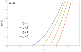
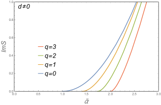
Figure 8: The imaginary part of the effective action as a function of $\tilde{\alpha}=E/E_{c}\left(0\right)$ in the D(-1)-D3 background. We have set $b=1$.

We can see that the decay rate becomes nonzero above the critical electric field $E_{c}$ and nearly independent on $q$ at sufficiently large electric field. We also note that the decay rate is suppressed in the presence of D-instantons which is in agreement with the analysis in the previous sections.

The D0-D4 case

In the D0-D4 background, the vacuum instability with an external electric field can be analyzed by following the discussion in the D(-1)-D3 background while the configuration of the D-branes is distinct as illustrated in Table 2.

	0	1	2	3	4	5$\left(z\right)$	6	7	8	9
D0-brane					-
D4-brane	-	-	-	-	-
D8-brane	-	-	-	-		-	-	-	-	-

Table 2: The configuration of the D-branes in the D0-D4 system.

The flavor brane is identified as a stack of D8- and anti D8-brane pair which is vertical to the D4-brane in the $x^{4}-z$ plane. In this configuration of the D-branes, the DBI action of a single pair of the flavor brane with nonzero components $F_{01}=E,F_{0z},F_{1z}$ of the gauge field strength can be written as,

$$S_{\mathrm{D8}} =-T_{\mathrm{D8}}\int d^{9}xe^{-\phi}\sqrt{-\det\left(g_{\mathrm{D8}}+2\pi\alpha^{\prime}F\right)}$$

$$=-\frac{2^{11}\pi^{2}}{3}T_{\mathrm{D}8}R^{12}V_{4}\int dz\frac{H_{0}^{3/2}}{z^{8}\sqrt{f}}\sqrt{\xi},$$ (5.9)

where

$$\xi=1-\frac{\left(2\pi\alpha^{\prime}\right)^{2}z^{6}}{64H_{0}R^{6}}\left[F_{01}^{2}+f\left(F_{0z}^{2}-F_{1z}^{2}\right)\right].$$ (5.10)

Then putting $\partial_{0}=0$ for the static electric field, we obtain the equations of motion as,

$$\partial_{z}\left(\frac{\sqrt{fH_{0}}}{z^{2}\sqrt{\xi}}F_{0z}\right) =0,\ \partial_{z}\left(\frac{\sqrt{fH_{0}}}{z^{2}\sqrt{\xi}}F_{1z}\right)=0,$$ (5.11)

which leads to two constants $j,d$ as current and charge, defined as,

$$j=2\pi\alpha^{\prime}\frac{\sqrt{fH_{0}}}{z^{2}\sqrt{\xi}}F_{1z},d=2\pi\alpha^{\prime}\frac{\sqrt{fH_{0}}}{z^{2}\sqrt{\xi}}F_{0z}.$$ (5.12)

Imposing (5.12) into (5.9), the effective action becomes,

$$S_{\mathrm{D8}}=-\frac{2^{11}\pi^{2}}{3}T_{\mathrm{D}8}R^{12}V_{4}\int dz\frac{H_{0}^{3/2}}{z^{8}\sqrt{f}}\sqrt{\left[1+\left(d^{2}-j^{2}\right)\frac{z^{10}}{64H_{0}^{2}R^{6}}\right]^{-1}\left[1-\frac{\left(2\pi\alpha^{\prime}E\right)^{2}z^{6}}{64H_{0}R^{6}}\right]},$$ (5.13)

and the stable current $j$ must be obtained by solving the constraints,

$$1+\left(d^{2}-j^{2}\right)\frac{z_{p}^{10}}{64H_{0}^{2}\left(z_{p}\right)R^{6}}=0,\ 1-\frac{\left(2\pi\alpha^{\prime}E\right)^{2}z_{p}^{6}}{64H_{0}\left(z_{p}\right)R^{6}}=0.$$ (5.14)

Afterwards we set $j=0$ to investigate the vacuum instability, the imaginary part of the effective action is therefore obtained as,

$$\mathrm{Im}S=-\frac{2^{11}\pi^{2}}{3}T_{\mathrm{D}8}R^{12}V_{4}\int_{z_{KK}}^{z_{*}}dz\frac{H_{0}^{3/2}}{z^{8}\sqrt{f}}\sqrt{\left(1+d^{2}\frac{z^{10}}{64H_{0}^{2}R^{6}}\right)^{-1}\left[\frac{\left(2\pi\alpha^{\prime}E\right)^{2}z^{6}}{64H_{0}R^{6}}-1\right]},$$ (5.15)

where $z_{*}$ is given as,

$$\frac{\left(2\pi\alpha^{\prime}E\right)^{2}z^{6}}{64H_{0}R^{6}}-1=\begin{cases}>0,&z\in\left[z_{*},z_{KK}\right],\\ <0,&z\in\left(0,z_{*}\right].\end{cases}$$ (5.16)

We numerically evaluate (5.15) as a function of $\tilde{\alpha}$ as illustrated in Figure 9.

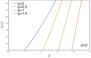
Figure 9: The imaginary part of the effective action as a function of $\tilde{\alpha}=E/E_{c}\left(0\right)$ in the D0-D4 background. The behavior of $\mathrm{Im}S$ is almost not affected by the value of $d$. We have set $b=1$.

While the exact behavior of the decay rate is a little different from the D(-1)-D3 case, our numerical calculation shows again that the decay rate is nonzero above the critical electric field $E_{c}$ and suppressed by the D-instantons. Obviously the behavior that the presence of D-instantons suppresses the decay rate is seemingly universal in the D-brane background with D-instantons.

6 Summary and discussion

In this work we have studied the Schwinger effect both in the confining D3- and D4-brane system with D-instantons. By using the DBI action of a probe brane, we find the critical electric field $E_{c}$ depends on the instanton density. Then we perform the potential analysis for the holographic Schwinger effect, calculate the total potential and the pair production rate for a pair of particle-antiparticle by taking into account an electric field. Afterwards we further investigate the electric instability with a single flavor and evaluate the associate flavor decay rate. According to our numerical calculation, we find the critical electric field is in agreement with the analysis of the DBI action. The presence of instantons increases the potential barrier and therefore suppresses the pair creation both in the D(-1)-D3 and D0-D4 approach. Our results agrees well with the evaluation obtained in the black D(-1)-D3 background at zero temperature limit [32] and the analysis for the flavor brane action in the D0-D4 background [33].

Finally let us give some physical interpretation of our results to close this work. The D(-1)-D3 case: Since the confining D(-1)-D3 system holographically corresponds to 3d Yang-Mills plus Chern-Simons theory below $M_{KK}$, in the dual field the particle may acquire effective topological mass through the Chern-Simons interaction due to the presence of the D(-1) branes (D-instantons) which means the particle mass is increased by the presence of the D-instantons. This would be more clear if we compute the propagator in the dual theory with a Chern-Simons term by using the method of quantum field theory, (2.3) which is,

$$\Delta_{\mu\nu}=\frac{p^{2}\eta_{\mu\nu}-p_{\mu}p_{\nu}-i\kappa g_{YM}^{2}\epsilon_{\mu\nu\rho}p^{\rho}}{p^{2}\left(p^{2}-\kappa^{2}g_{YM}^{4}\right)}+\mathrm{gauge\ term},$$ (6.1)

leading to a topological mass $\Delta m=\kappa g_{YM}^{2}$. Therefore the particle creation in Schwinger effect would be suppressed by the D-instantons since it is proportional to the factor $e^{-\frac{m^{2}}{E}}$. Or namely, the barrier of total potential for a pair of particle-antiparticle is increased by the presence of the D-instantons which is consistent with what we have obtained in this work. The Schwinger effect with D-instantons might be very helpful to investigate some phenomena in 3d Maxwell-Chern-Simons theory with electric field e.g. the phase transition from insulator to conductor in some material.

The D0-D4 case: According to the previous study in this system [27, 29, 30, 31, 36, 41, 42], the dual field theory is confining Yang-Mills theory with a theta term (D-instanton density) and the particle mass spectrum is increased by the presence of the D-instantons (D0-branes). Hence the particle creation in Schwinger effect should also be suppressed or namely the total potential barrier is increased by the instantons which is consistent with the holographic analysis in this work. The total potential with D-instantons in Schwinger effect would be also remarkable to study the P or CP violation in QCD, especially in the heavy-ion collision, since an extremely strong electromagnetic field would be generated. On the other hand, in the collision, there might be a metastable state with nonzero vacuum theta angle produced in the hot and dense condition when the deconfinement phase transition happens [8, 9]. Therefore the metastable state may be excited by the strong electric field through the Schwinger effect and the particle pair creation in the heavy-ion collision would be affected by the theta angle (D-instantons), reflecting the behaviors of the total potential. So Schwinger effect with D-instantons might be an observable phenomenon to confirm whether P or CP violation in QCD exists.

References

- [1] J. S. Schwinger, “On gauge invariance and vacuum polarization,” Phys. Rev. 82 (1951) 664.
- [2] I. K. Affleck, O. Alvarez and N. S. Manton, “Pair Production At Strong Coupling In Weak External Fields,” Nucl. Phys. B 197 (1982) 509.
- [3] Ettore Vicari, Haralambos Panagopoulos, “Theta dependence of SU(N) gauge theories in the presence of a topological term”, Phys. Rept. 470, 93 (2009) [arXiv:0803.1593 [hep-th]].
- [4] Massimo D’Elia, Francesco Negro, “Theta dependence of the deconfinement temperature in Yang-Mills theories”, PhysRevLett.109.07200, [arXiv:1205.0538].
- [5] Massimo D’Elia, Francesco Negro, “Phase diagram of Yang-Mills theories in the presence of a theta term”, Phys. Rev. D 88, 034503 (2013), [arXiv:1306.2919].
- [6] Edward Witten, “Theta Dependence In The Large N Limit Of Four-Dimensional Gauge Theories”, Phys.Rev.Lett.81:2862-2865,1998, [arXiv:hep-th/9807109].
- [7] Luigi Del Debbio, Gian Mario Manca, Haralambos Panagopoulos, Apostolos Skouroupathis, Ettore Vicari, “Theta-dependence of the spectrum of SU(N) gauge theories”, JHEP 0606:005,2006, [arXiv:hep-th/0603041].
- [8] Dmitri Kharzeev, R.D. Pisarski, Michel H.G. Tytgat, “Possibility of spontaneous parity violation in hot QCD”, Phys.Rev.Lett. 81 (1998) 512-515, [arXiv:hep-ph/9804221].
- [9] K. Buckley, T. Fugleberg, A. Zhitnitsky, “Can theta vacua be created in heavy ion collisions?”, Phys.Rev.Lett. 84 (2000) 4814-4817, [arXiv:hep-ph/9910229].
- [10] D. Kharzeev, “Parity violation in hot QCD: why it can happen, and how to look for it”, Physletb.2005.11.075, [arXiv:hep-ph/0406125].
- [11] Dmitri E. Kharzeev, Larry D. McLerran, Harmen J. Warringa, “The effects of topological charge change in heavy ion collisions: “Event by event P and CP violation”, Nucl.Phys.A803: 227-253, 2008, [arXiv: 0711.0950].
- [12] Kenji Fukushima, Dmitri E. Kharzeev, Harmen J. Warringa, “The Chiral Magnetic Effect”, PhysRevD.78.074033, [arXiv:0808.3382].
- [13] Dmitri E. Kharzeev, “The Chiral Magnetic Effect and Anomaly-Induced Transport”, j.ppnp.2014.01.002, [arXiv:1312.3348].
- [14] J. M. Maldacena, “The large N limit of superconformal field theories and supergravity,” Adv. Theor. Math. Phys. 2, 231 (1998) [Int. J. Theor. Phys. 38, 1113 (1999)] [arXiv:hep-th/9711200].
- [15] Edward Witten, “Anti De Sitter Space And Holography”, Adv.Theor.Math.Phys.2:253-291,1998, [arXiv:hep-th/9802150].
- [16] Gordon W. Semenoff, Konstantin Zarembo, “Holographic Schwinger Effect”, Phys.Rev.Lett. 107 (2011) 171601, [arXiv:1109.2920].
- [17] Edward Witten, “Anti-de Sitter space, thermal phase transition, and confinement in gauge theories”, Adv.Theor.Math.Phys. 2 (1998) 505-532, [arXiv:hep-th/9803131].
- [18] Katrin Becker, Melanie Becker, John H. Schwarz, “String theory and M-theory, A Modern Introduction”, Cambridge University Press, 2007.
- [19] Y. Sato and K. Yoshida, “Potential Analysis in Holographic Schwinger Effect”, JHEP 08 (2013) 002, arXiv:1304.7917 [hep-th].
- [20] Yoshiki Sato, Kentaroh Yoshida, “Holographic Schwinger effect in confining phase”, JHEP 09 (2013) 134, [arXiv:1306.5512].
- [21] Daisuke Kawai, Yoshiki Sato, Kentaroh Yoshida, “Schwinger pair production rate in confining theories via holography”, Phys.Rev.D 89 (2014) 10, 101901, [arXiv:1312.4341].
- [22] Hong Liu, Arkady A. Tseytlin, “D3-brane D instanton configuration and N=4 superYM theory in constant selfdual background”, Nucl.Phys.B 553 (1999) 231-249, [arXiv:hep-th/9903091].
- [23] Bogeun Gwak, Minkyoo Kim, Bum-Hoon Lee, Yunseok Seo, Sang-Jin Sin, “Holographic D Instanton Liquid and chiral transition”, Phys.Rev.D 86 (2012) 026010, [arXiv:1203.4883].
- [24] Si-wen Li, Shu Lin, “D-instantons in Real Time Dynamics”, Phys.Rev.D 98 (2018) 6, 066002, [arXiv:1711.06365].
- [25] Si-wen Li, Sen-kai Luo, Mu-zhi Tan, “Three-dimensional Yang-Mills Chern-Simons theory from D3-brane background with D-instantons”, [arXiv: 2106.04038].
- [26] Kenji Suzuki, “D0-D4 system and QCD(3+1)”, Phys.Rev.D 63 (2001) 084011, [arXiv:hep-th/0001057].
- [27] Chao Wu, Zhiguang Xiao, Da Zhou, “Sakai-Sugimoto model in D0-D4 background”, Phys.Rev.D 88 (2013) 2, 026016, [arXiv:1304.2111].
- [28] Shigenori Seki, Sang-Jin Sin, “A New Model of Holographic QCD and Chiral Condensate in Dense Matter”, JHEP 10 (2013) 223, [arXiv:1304.7097].
- [29] Lorenzo Bartolini, Francesco Bigazzi, Stefano Bolognesi, Aldo L. Cotrone, Andrea Manenti, “Theta dependence in Holographic QCD”, JHEP 02 (2017) 029, [arXiv:1611.00048].
- [30] Francesco Bigazzi, Aldo L. Cotrone, Roberto Sisca, “Notes on Theta Dependence in Holographic Yang-Mills”, JHEP 08 (2015) 090, [arXiv:1506.03826].
- [31] Si-Wen Li, “A holographic description of theta-dependent Yang-Mills theory at finite temperature”, Chin.Phys.C 44 (2020) 1, 013103, [arXiv:1907.10277].
- [32] Leila Shahkarami, Majid Dehghani, Parvin Dehghani, “Holographic Schwinger Effect in a D-Instanton Background”, Phys.Rev.D 97 (2018) 4, 046013, [arXiv:1511.07986].
- [33] Wenhe Cai, Kang-le Li, Si-wen Li, “Electromagnetic instability and Schwinger effect in the Witten–Sakai–Sugimoto model with D0–D4 background”, Eur.Phys.J.C 79 (2019) 11, 904, [arXiv:1612.07087].
- [34] Juan Maldacena, “Wilson loops in large N field theories”, Phys.Rev.Lett. 80 (1998) 4859-4862, [hep-th/9803002].
- [35] Yoshiki Sato, Kentaroh Yoshida, “Universal aspects of holographic Schwinger effect in general backgrounds”, JHEP 12 (2013) 051, [arXiv:1309.4629].
- [36] Si-wen Li, Tuo Jia, “Matrix model and Holographic Baryons in the D0-D4 background ”, Phys.Rev.D 92 (2015) 4, 046007, [arXiv:1506.00068].
- [37] Koji Hashimoto, Takashi Oka, Akihiko Sonoda, “Electromagnetic instability in holographic QCD”, JHEP 1506 (2015) 001, [arXiv:1412.4254].
- [38] Koji Hashimoto, Takashi Oka, Akihiko Sonoda, “Magnetic instability in AdS/CFT : Schwinger effect and Euler-Heisenberg Lagrangian of Supersymmetric QCD”, JHEP 1406 (2014) 085, [arXiv:1403.6336].
- [39] Koji Hashimoto, Takashi Oka, “Vacuum Instability in Electric Fields via AdS/CFT: Euler-Heisenberg Lagrangian and Planckian Thermalization”, JHEP 1310 (2013) 116, [arXiv:1307.7423].
- [40] A. Karch and E. Katz, “Adding flavor to AdS / CFT”, JHEP 0206 (2002) 043, arXiv: hep- th/0205236.
- [41] Si-wen Li, Tuo Jia, “Three-body force for baryons from the D0-D4/D8 brane matrix model”, Phys.Rev.D 93 (2016) 6, 065051, [arXiv:1602.02259].
- [42] Wenhe Cai, Chao Wu, Zhiguang Xiao, “Baryons in the Sakai-Sugimoto model in the D0-D4 background”, Phys.Rev.D 90 (2014) 10, 106001, [arXiv:1410.5549].