A stochastic differential equation approach to the analysis of the UK 2017 and 2019 general election polls

Abstract

Human dynamics and sociophysics build on statistical models that can shed light on and add to our understanding of social phenomena. We propose a generative model based on a stochastic differential equation that enables us to model the opinion polls leading up to the UK 2017 and 2019 general elections, and to make predictions relating to the actual result of the elections. After a brief analysis of the time series of the poll results, we provide empirical evidence that the gamma distribution, which is often used in financial modelling, fits the marginal distribution of this time series. We demonstrate that the proposed poll-based forecasting model may improve upon predictions based solely on polls. The method uses the Euler-Maruyama method to simulate the time series, measuring the prediction error with the mean absolute error and the root mean square error, and as such could be used as part of a toolkit for forecasting elections.

Keywords: election polls; forecasting elections; time series; stochastic differential equations; CIR process; gamma distribution; Euler-Maruyama method.

1 Introduction

We propose to model election polls as a time series [Chatfield and Xing, 2019], motivated by [Wlezien and Erikson, 2002], who considered modelling the sequence of polls as an autoregressive process. Poll-based election forecasting methods [Fisher, 2018], building on vote-intention polls, play an important role in the endeavour to predict the outcome of an election; see Section 2 for a brief review on the methods of forecasting elections. We demonstrate that the model we propose, based on stochastic differential equations (SDEs) [Mackevicius, 2011, Evans, 2013], has the potential to give better predictions of the actual election result than simply using the results of the polls themselves.

In particular, we present a companion paper to [Fenner et al., 2018] using the same methodology, which is based on SDEs applied to opinion polls leading up to an election rather than to a referendum. We deploy a novel stochastic process based on the Cox-Ingersoll-Ross (CIR) process [Cox et al., 1985, Chou and Lin, 2006], used to model the term structure of interest rates [Berk and DeMarzo, 2017]. CIR processes are ‘mean-reverting’ diffusion processes [Hirsa and Neftci, 2014], and have marginal distributions which are gamma distributed. Moreover, processes that are sums of such diffusions have autocorrelation functions (also known as serial correlation functions) that are sums of the exponentially decaying autocorrelation functions of the constituent diffusion processes [Bibby et al., 2005, Forman and Sørensen, 2008], allowing the approximation of heavy tailed distributions [Feldman and Whitt, 1998].

We refer the reader to [Fenner et al., 2018] for the background in human dynamics and sociophysics [Sen and Chakrabarti, 2014] (also known as social physics), noting that statistical physics [Castellano et al., 2009] has played a central role in its formulation; humans are viewed as “social atoms”, each exhibiting simple individual behaviour having limited complexity, but nevertheless collectively they yield complex social patterns [Levene et al., 2019]. In the context of human dynamics, the SDE model we propose is a generative model in the form of a stochastic process the evolution of which gives rise to distributions such as power law and Weibull distributions [Fenner et al., 2015]. Generative models also arise from agent-based models [Conte and Paolucci, 2014] and have played an important role in the sociophysics literature in the context of opinion dynamics [Castellano et al., 2009, Sîrbu et al., 2017]. In particular, the voter model and its extensions [Castellano et al., 2009, Sîrbu et al., 2017], whereby at each time step an agent decides whether to hold on to or change its opinion depending on the opinions of its neighbours, have applications in explaining and understanding voting behaviour during elections.

Opinion polls, which provide the data source for our SDE model, relay important information to the public in the lead-up to an election and provide an important ingredient of forecasting methods; see [Traugott and Lavrakas, 2016] for a high-level overview of election polls. In a given election cycle, polls can be naturally viewed as a time series, and thus be expected to follow a stochastic process, such as an autoregressive model of order 1 (or more succinctly an AR(1) model) [Chatfield and Xing, 2019]. In [Wlezien and Erikson, 2002] the authors had some reservations about using such a time series model, due to sampling error and lack of sufficient time series data, and thus proposed to analyse the data in terms of a time series cross-sectional model [Beck and Katz, 2011], treating data as cross sections for each time unit in the election cycle. Furthermore, in [Wlezien et al., 2017] it was mentioned that, given a sufficient number of poll results, these could be readily treated as a statistical time series. The availability of a sufficient number of polls, in our case leading up to the 2017 and 2019 UK general elections, and a more general stochastic model, such as the one we propose, allow for the resurrection of poll-based forecasting using time series.

In [Fenner et al., 2018] we took a fresh look at the time series approach, going beyond the model suggested in [Wlezien and Erikson, 2002], and made use of the availability of a large number of polls conducted at regular intervals. In particular, we proposed a novel model based on SDEs, which are widely used in physics and mathematical finance to model diffusion processes, that can be viewed as continuous approximations to discrete processes modelling how the polls vary over time. Therein we provided empirical evidence that the beta distribution, which is a natural choice when modelling proportions, fits the marginal distribution of the time series and we provided evidence of the predictive power of the model (cf. [Kononovicius, 2017, Mori et al., 2019]). One disadvantage of this model is that its autocorrelation function is decreases exponentially [Bibby et al., 2005], while in reality the tails of the autocorrelation function may be heavier. We address this problem in Section 4 by extending the model of [Fenner et al., 2018] to allow processes that are sums of diffusions [Bibby et al., 2005, Forman and Sørensen, 2008], in which case the autocorrelation function is a sum of exponentials.

In order to evaluate the predictive power of the model, we make use of the Euler-Maruyama (EM) method [Sauer, 2013], which is a computational method for approximating numerical solutions to SDEs. In particular, the EM method allows us to simulate the time series in order to predict the result of the election from the SDEs. We utilise the well-known mean absolute error (MAE) and root mean square error (RMSE) metrics [Chai and Draxler, 2014] to assess the accuracy of the EM method in predicting the actual election result, and we compare these to the predictions obtained by simply taking the results of the opinion polls; see [Jennings et al., 2020] for a discussion on the use MAE and RMSE for assessing the forecasting performance of polls.

The rest of the paper is organised as follows. In Section 2, we review related research on election forecasting. In Section 3, we provide a brief analysis of the UK election poll results for 2017 and 2019. In Section 4, we propose a generative model for analysing the polling data based on a sum of ‘mean-reverting’ stochastic differential equations. In Section 5, we apply the model to the polls leading up to the UK 2017 and 2019 general elections, utilising the EM method to evaluate the predictive power of the model. Finally, in Section 6, we give our concluding remarks.

2 A brief review of forecasting elections and previous research

Forecasting election results focuses the mind on what is important in influencing election outcomes [Fisher, 2018]. Its goal is clear, to predict which party will win the elections. Here will only consider two-party systems and, in particular, we examine the contest between the Conservative and Labour parties in the UK; however, the model we present is also relevant to other two-party systems such as in the USA, where the contest is between the Republicans and Democrats. Although in election forecasting, the task at hand is to predict the winner, it is also about understanding how elections work and how effective the proposed models really are.

We now briefly outline the prominent election forecasting methods. Structural models are based on fitting a regression model [Gelman et al., 2020] to historical election data and using the results for prediction, assuming a causal relationship exists between the past and present. The independent variables, or predictors, are referred to as fundamentals, and most often include economic indicators (i.e. how did the economy perform) and leadership evaluations (i.e. how did the leaders perform).

As opposed to structural models, poll-based forecasting is based on voter intention. Two main challenges of poll-based forecasting are: how to aggregate polls and what model to use for the actual forecasting [Pasek, 2015, Jackson, 2016]. Early approaches using time series to model polls for the purpose of building predictive models, were proposed by [Erikson and Wlezien, 1999] and [Green et al., 1999]. Both of these models were especially concerned with reducing the sampling error of polls, and thereby with methods for smoothing the time series data.

Our focus is on the forecasting model itself rather than in aggregation, and to this end modelling the polls as a time series like in those early approaches mentioned above. However, we view the time series of polls as a diffusion process, which is a continuous approximation to discrete processes modelling the changes to polls over time. In particular, we propose to use ‘mean-reverting’ diffusion processes arising from a particular class of SDEs [Bibby et al., 2005], which describe CIR processes [Cox et al., 1985]. Using the Euler-Maruyama method, mentioned in the introduction, the continuous SDEs of the CIR process are approximated by discrete processes analogous to the AR(1) process [Chatfield and Xing, 2019], as suggested in [Wlezien and Erikson, 2002]. The model we propose, is however ‘mean reverting’ and thus possesses a stationary solution. Moreover, the marginal distribution of the solution is a gamma distribution [Cobb, 1981, Bibby et al., 2005], an aspect which is further discussed in Section 4.

It is important to note that polls are not a panacea for forecasting election outcomes, and they may fail to provide accurate predictions, as in the 2015 UK elections where the polling samples were unrepresentative of the target population’s voting intentions [Sturgis et al., 2018]. We also mention that the model presented in [Ford et al., 2016], which includes the aggregation of polls from various sources, taking into account historical polling data used to calibrate the prediction, and also provides, through simulation, UK constituency-level forecasts. Furthermore, it was demonstrated in [Wlezien and Erikson, 2002, Wlezien et al., 2017] that, as one would expect, polls are generally more accurate the closer they are in the election cycle to the actual election. Synthetic models [Lewis-Beck et al., 2016], and, more generally hybrid models [Pasek, 2015] combine poll-based and structural models to obtain the advantages of both. One such example is the model of [Linzer, 2013], which proposes a synthetic dynamic Bayesian model that provides both national-level and state-level forecasts.

Prediction markets provide another data source for forecasters, with the argument that in this case, since people are betting on the result, they will take all available information into account. However, it is not clear whether prediction markets perform better than polls. In [Reade and Vaughan Williams, 2019] the authors concluded that opinion polls are favourable in terms of their bias (the mean error of all forecasts), while prediction markets are better in terms of their precision (the reciprocal of the variance of all forecasts).

Citizen forecasting is the process of aggregating forecasts made by individuals, which can be viewed as a form of ‘wisdom of crowds’. While polls are based on voters intentions, citizen forecasting is based on voter expectations. In [Murr et al., 2021], empirical evidence is provided that election forecasts based on voter expectation outperform those based on voter intention. In general, it would advisable to augment poll-based prediction with voter expectation surveys, should they become readily available. In principle, the techniques used for polls, as the one suggested herein, could be easily adapted to expectation surveys. Furthermore, combining any number of the forecasting methods discussed, and weighting them according to their perceived accuracy, may lead to more accurate forecasts [Graefe et al., 2014].

Another way to distinguish between forecasts, proposed by [Lewis-Beck and Tien, 2016] is to contrast the long view with the short view. Taking the long view, performance is examined over several election contests and forecasts are made well before election day, while in the short view performance is measured iteratively and depends increasingly on polls as election day gets closer. Here we take the short view based solely on polls, however we note that synthetic models, which combine both views, can mitigate against inaccurate polling.

Another method, which has become popular due to the availability of social media data is nowcasting [Ceron et al., 2017], a method whose aim is to predict the present or the very near present, rather than the future. So, suppose that social media data are available, such as textual content from Twitter. Then, using this data, sentiment analysis [Liu, 2015] of the text can be computed, and, if it indicates a positive intention to vote for a particular party, this information can, in principle, be used in lieu of polling information. Moreover, since past Twitter data are available, they may also be combined into a time series and employed for forecasting, using, for example, the model we propose.

3 Preliminary analysis of the time series of poll results

The analysis for the 2017 election was carried out using the results of 254 opinion polls, which were collected prior to the election that took place on 8th June 2017. The data set was obtained online from [Financial Times, 2017], the first poll being taken on 9th May 2015 and the last on the day before the election. Detailed results of the election can be obtained online from [BBC, 2017]. Similarly, the analysis for the 2019 election was carried out using the results of 568 opinion polls, which were collected prior to the election that took place on 12th December 2019. The data set was obtained online from [Financial Times, 2019], the first poll being taken on 4th January 2017 and the last on the day before the election. Detailed results of the election can be obtained online from [BBC, 2019]. For each party and for each election, the data set used was a time series of the proportion of respondents who said they would vote for that party. These are shown graphically in Figures 1 and 2; the minimum and maximum values of the intended vote share, for the Conservative and Labour parties, over all the 2017 and 2019 polls are shown in Tables 1 and 2, respectively.

2017 elections	Min	Max
Conservative	30%	50%
Labour	23%	40%

Table 1: Minimum and maximum percentages of the intended vote share from the 2017 polls.

2019 elections	Min	Max
Conservative	17%	50%
Labour	18%	46%

Table 2: Minimum and maximum percentages of the intended vote share from the 2019 polls.

When analysing the data, in order to detect any clear trends, it is interesting to inspect the moving averages [Chatfield and Xing, 2019] of the polls, which are shown in Figures 1 and 2. For the 2017 election, it is clear that, although there was a dip in the support for Labour as the election was approaching, as it got closer to the election date the gap between Conservative and Labour narrowed, until the last day before the election when the Conservative lead in the polls was only 1%. In the election itself, where the actual result was that the Conservatives received 42.4% of the vote and Labour 40.0%, the Conservative lead was slightly higher at 2.4%. In 2019, the election date of 12th December was decided in parliament on the 29th October, and the Conservative lead in the polls from that date until the election was on average 10.8%, with a standard deviation of 3.37%. The Conservative lead on the last day before the elections was 11% and in the election itself, in which the actual result was that the Conservatives received 43.6% of the vote and Labour 32.2%, the lead was even higher at 11.4%. This does not tell the whole story of this election as the UK “first-pass-the-post” electoral system resulted in the Conservatives ending up with a majority of 80 seats in parliament.

In our model and analysis given below we treat the two parties and two elections independently, with the realisation that in practice the time series for the Conservatives and Labour parties are not actually independent and that there may be dependencies between consecutive elections; we view our model and analysis as a first approximation to the poll-based forecasting problem. We note that although the two main parties in the UK receive most of the votes, there is at least a third party, the Liberal Democrats, which we have not considered in this analysis, but could be considered in future research. In this context, it is worth noting that there have been times when one of the two main parties receives more votes, possibly at the expense of the other (see Figure 1), and there are other times when both of the parties have received more votes, possibly at the expense of a third party (see Figure 2).

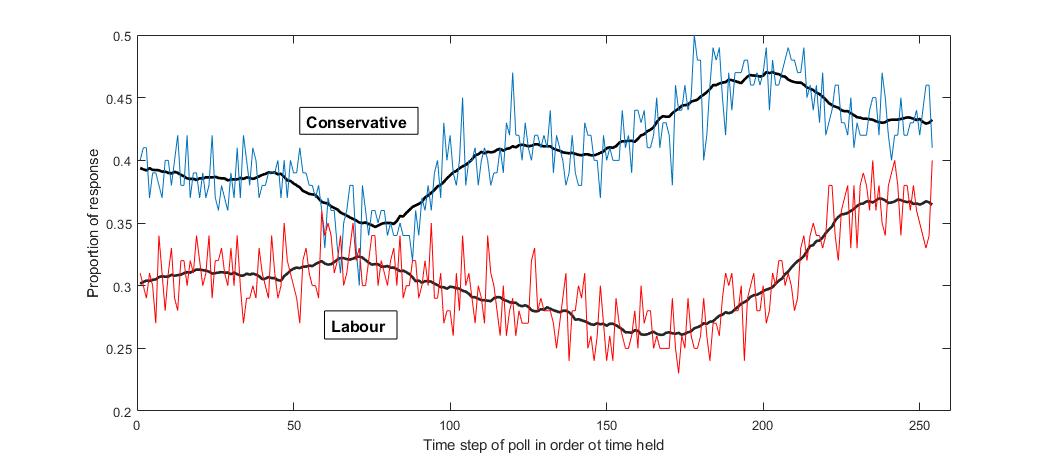
Figure 1: Raw time series and moving averages of the 2017 polls with a centred sliding window of 25 time steps for the Conservative and Labour parties.

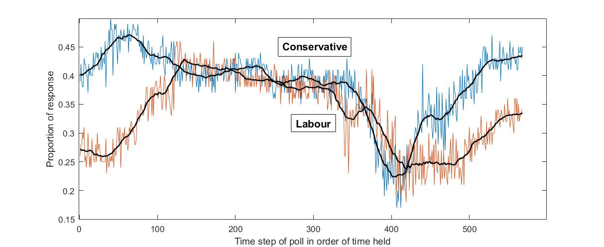
Figure 2: Raw time series and moving averages of the 2019 polls with a centred sliding window of 25 time steps for the Conservative and Labour parties.

4 A generative model for time series with application to polls

Stochastic differential equations can provide effective generative models for time series. In particular, when the SDEs are ‘mean-reverting’ [Hirsa and Neftci, 2014], as will be the case here, they often possess stationary solutions that fit a number of well-studied distributions [Cobb, 1981, Bibby et al., 2005]. In our application, analysing the poll results, the gamma distribution [Johnson et al., 1994, Dagpunar, 2019] appears to be a natural choice, since it is flexible and allows the construction of a sum of diffusion processes having an autocorrelation function that is a sum of exponentials [Bibby et al., 2005, Forman and Sørensen, 2008].

A typical stochastic differential equation (SDE) takes the form

$${\mathrm{d}}X_{t}=\mu(X_{t}){\mathrm{d}}t+\sigma(X_{t}){\mathrm{d}}W_{t},$$ (1)

where $X_{t}$ is a random variable with $t\geq 0$ a real number denoting time; $\mu$ and $\sigma$ are known as the drift and diffusion functions, respectively, and $W_{t}$ is a Wiener process (also known as Brownian motion). Moreover, when

$$\mu(x)=\theta\left(m-x\right),$$ (2)

where $\theta$, the rate parameter, is a positive constant and $m$ is a constant representing the mean of the underlying stochastic process, the SDE has a stationary solution [Cobb, 1981, Bibby et al., 2005]. In addition, its autocorrelation function is exponentially decreasing [Bibby et al., 2005] and takes the form

$$\exp(-\theta t).$$ (3)

Such a stochastic process is known as a ‘mean-reverting’ process. It was shown in [Cobb, 1981, Bibby et al., 2005] that, if

$$\sigma^{2}(x)=\frac{2\theta}{\lambda}x$$ (4)

and $\lambda$ is defined by

$$m=\frac{\alpha}{\lambda},$$ (5)

the marginal distribution of the stationary solution of the SDE is a gamma distribution [Johnson et al., 1994] with probability density function

$$\frac{\lambda^{\alpha}}{\Gamma(\alpha)}x^{\alpha-1}\exp(-\lambda x),$$ (6)

where $\Gamma$ is the gamma function [Abramowitz and Stegun, 1972, 6.1]; $\alpha>0$ is the shape of the distribution and $\lambda>0$ is a scale parameter. We note that several other forms for $m$ and $\sigma^{2}(X_{t})$ also lead to well-known distributions [Cobb, 1981, Bibby et al., 2005].

Under the above conditions, substituting (4) and (5) into (1) gives the SDE

$${\mathrm{d}}X_{t}=\theta\left(\frac{\alpha}{\lambda}-X_{t}\right){\mathrm{d}}t+\sqrt{\frac{2\theta}{\lambda}X_{t}}\ {\mathrm{d}}W_{t},$$ (7)

which describes a process called the Cox-Ingersoll-Ross process (CIR process) [Cox et al., 1985]. From the results in [Feller, 1951] (cf. [Cox et al., 1985]), we can conclude that the solution to (7) is positive when $\alpha\geq 1$.

The autocorrelation function of the CIR process is exponential as in (3), and therefore, in order to model a process having an autocorrelation function with a heavier tail (such as a power law), we introduce a diffusion process that is a sum of CIR processes [Bibby et al., 2005, Forman and Sørensen, 2008], for which the autocorrelation function is a sum of exponentials. This relies on the result that a power law can be approximated by a finite sum of exponentials, since it is a completely monotone function [Feldman and Whitt, 1998] (cf. [Fenner et al., 2016]).

We can obtain a process $X_{t}$ as the sum of $n$ processes by letting

$$X_{t}=X_{t}^{(1)}+X_{t}^{(2)}+\cdots+X_{t}^{(n)},$$ (8)

where the Wiener processes $W_{t}^{(i)}$ are independent, for $1\leq i\leq n$, and $X_{t}^{(i)}$ is defined by the SDE

$${\mathrm{d}}X_{t}^{(i)}=\theta_{i}\left(\frac{\phi_{i}\alpha}{\lambda}-X_{t}^{(i)}\right){\mathrm{d}}t+\sqrt{\frac{2\theta_{i}}{\lambda}X_{t}^{(i)}}\ {\mathrm{d}}W_{t}^{(i)}.$$ (9)

Then the mean, diffusion squared and autocorrelation function are given, respectively, by

$$m_{i}=\frac{\phi_{i}\alpha}{\lambda},\quad\sigma^{2}\left(X_{t}^{(i)}\right)=\frac{2\theta_{i}}{\lambda}X_{t}^{(i)}\ \ {\rm and}\quad\exp(-\theta_{i}t),$$ (10)

where

$$\phi_{1}+\phi_{2}+\cdots+\phi_{n}=1.$$ (11)

It follows that the marginal distribution of each $X_{t}^{(i)}$ is a gamma distribution with shape $\phi_{i}\alpha$ and scale parameter $\lambda$. The marginal distribution of the sum $X_{t}$ is a gamma distribution with shape $\alpha$ and the same scale parameter $\lambda$. Moreover, $X_{t}$ has autocorrelation function

$$\phi_{1}\exp(-\theta_{1}t)+\phi_{2}\exp(-\theta_{2}t)+\cdots+\phi_{n}\exp(-\theta_{n}t).$$ (12)

5 Analysis of the poll results for the general elections

The approach we have taken to validate the model is similar to that taken in [Taufer, 2007], building on the stationary diffusion-type models developed in [Bibby et al., 2005] for constructing diffusion processes with a given marginal distribution and autocorrelation function.

We can simulate the sum of the diffusion processes defined by (8) and (9) using the Euler-Maruyama (EM) method [Sauer, 2013] (cf. [Dereich et al., 2012]), which is a general computational method for obtaining approximate numerical solutions to SDEs. We also make use of the Jensen-Shannon divergence ($JSD$) [Endres and Schindelin, 2003] as a goodness-of-fit measure [Levene and Kononovicius, 2019]. All computations were carried out using the Matlab software package.

In Tables 3 and 4 we show the parameters of the gamma distributions fitted to the data sets using the maximum likelihood method, and the $JSD$ between the empirical marginal distribution of the time series of the poll results and the fitted gamma distribution; we note that its mean $\mu$ is given by $\mu=\alpha/\lambda$, and its standard deviation $\sigma$ by $\sigma^{2}=\alpha/\lambda^{2}$. The low $JSD$ values indicate good fits for both political parties. We note that the $JSD$ for the Conservative party in the 2019 elections is much higher than that for 2017, which could indicate that another distribution may better fit the data. In fact, we found that the Gumbel distribution [Johnson et al., 1995, Kotz and Nadarajah, 2000] (also known as a type I extreme value distribution) is a better fit for the Conservatives in 2019, with $JSD$ of $0.0595$, although a worse fit for Labour in 2019 with a $JSD$ of $0.0801$. We also note that, on inspection of Tables 1 and 2, it would seem that employing a truncated gamma distribution [Zaninetti, 2013] would lead to a more accurate, albeit more complex, model. We leave these lines of investigation for future work as, for the purpose of prediction, the gamma distribution seems to be sufficient.

2017 elections	$\alpha$	$\lambda$	$\mu$	$\sigma$	$JSD$
Conservative	105.8670	258.5847	0.4094	0.0398	0.0370
Labour	72.0295	236.1929	0.3050	0.0359	0.0478

Table 3: Maximum likelihood fitting of the gamma distribution to the 2017 election polls.

2019 elections	$\alpha$	$\lambda$	$\mu$	$\sigma$	$JSD$
Conservative	32.0520	83.0583	0.3859	0.0682	0.1117
Labour	25.2832	75.8911	0.3332	0.0663	0.0470

Table 4: Maximum likelihood fitting of the gamma distribution to the 2019 election polls.

We fit the autocorrelation function in (12), for $n=2$, using least squares nonlinear regression in order to obtain estimates $\phi_{i}$ and $\theta_{i}$, for $i=1,2$. The results for the 2017 and 2019 poll results are shown in Tables 5 and 6, respectively, where we first smoothed the autocorrelations using a moving average with a window of length two. For comparison purposes we also show in Tables 7 and 8, fits for a single exponential, i.e. when $n=1$, for 2017 and 2019, respectively, which are worse than the fits for a mixture of two exponentials, i.e. when $n=2$.

2017 elections	$\phi_{1}$	$\theta_{1}$	$\phi_{2}$	$\theta_{2}$	$JSD$
Conservative	0.8092	0.0146	0.1908	0.9896	0.0074
Labour	0.7509	0.0237	0.2491	1.1890	0.0179

Table 5: Parameters of the exponential sum autocorrelation for the 2017 election polls.

2019 elections	$\phi_{1}$	$\theta_{1}$	$\phi_{2}$	$\theta_{2}$	$JSD$
Conservative	0.9717	0.0089	0.0283	2.3243	0.0035
Labour	0.9439	0.0066	0.0561	1.1521	0.0025

Table 6: Parameters of the exponential sum autocorrelation for the 2019 election polls.

2017 elections	$\phi_{1}$	$\theta_{1}$	$JSD$
Conservative	0.8702	0.0202	0.0206
Labour	0.8298	0.0317	0.0324

Table 7: Parameters of the single exponential autocorrelation for the 2017 election polls.

2019 elections	$\phi_{1}$	$\theta_{1}$	$JSD$
Conservative	0.9775	0.0094	0.0043
Labour	0.9592	0.0078	0.0056

Table 8: Parameters of the single exponential autocorrelation for the 2019 election polls.

We now turn our attention to the widely used mean absolute error (MAE) and root mean square error (RMSE) evaluation metrics [Chai and Draxler, 2014], in order to directly estimate the prediction of the actual result using the EM method. The MAE is given by

$$MAE=\frac{\sum_{j=1}^{m}|p_{j}-f|}{m},$$ (13)

where $p_{j}$ is the proportion favouring a political party in the $j$th poll, $f$ is the corresponding proportion of votes in the actual election, and $m$ is the number of polls. The RMSE is given by

$$RMSE=\sqrt{\frac{\sum_{j=1}^{m}\left(p_{j}-f\right)^{2}}{m}},$$ (14)

noting that it is at least as large as the MAE.

We use the first third of the polls for computing the initial model parameter values, $\alpha$ and $\lambda$, of the gamma distribution, and also the $\phi_{i}$ and rate parameters $\theta_{i}$ in (12), with $n=2$. For each of the remaining two thirds of the polls, we adjust the parameters and use the EM method to predict the next step in the time series. We repeat this twenty times and take the average of the twenty predictions at each time step to get the average prediction, and also compute the prediction when we set ${\mathrm{d}}W_{t}^{(i)}$ to zero in (9), which is what we would expect the average to converge to when increasing the number of EM computations, effectively eliminating the random component of the SDE represented by the diffusion function. We then compare the average prediction to the actual result of the election. We evaluate the accuracy of the predictions over the complete range using the MAE and RMSE. For comparison purposes, we also computed the MAE and RMSE using the current poll (the most recent poll inspected by the prediction algorithm) as the predictor of the actual result; these are shown in Tables 9 and 10 in the columns labelled MAE-polls and RMSE-polls. The columns labelled MAE-EM and RMSE-EM show the error values of the predictions made using the EM method. It can be seen from these that for the two parties in both 2017 and 2019 the EM method was a better predictor than the polls themselves, and that the results in both tables are comparable; the margin of improvement is greatest for the Conservatives in 2019.

Party-Year/Metric	MAE-polls	RMSE-polls	MAE-EM	RMSE-EM
Con 2017	0.0278	0.0348	0.0245	0.0294
Lab 2017	0.0988	0.1072	0.0951	0.0981
Con 2019	0.0719	0.0949	0.0644	0.0853
Lab 2019	0.0532	0.0618	0.0491	0.0568

Table 9: MAE and RMSE prediction errors for the 2017 and 2019 UK election results when averaging the predictions over twenty runs of the EM method. (The smaller error values are italicised.)

Party-Year/Metric	MAE-polls	RMSE-polls	MAE-EM	RMSE-EM
Con 2017	0.0278	0.0348	0.0250	0.0296
Lab 2017	0.0988	0.1072	0.0951	0.0977
Con 2019	0.0719	0.0949	0.0641	0.0850
Lab 2019	0.0532	0.0618	0.0486	0.0563

Table 10: MAE and RMSE prediction errors for the 2017 and 2019 UK election results, when we set ${\mathrm{d}}W_{t}^{(i)}=0$. (The smaller error values are italicised.)

We also counted the number of times the prediction using EM method was closer to the actual election result than was the prediction based on the current poll, and vice versa (cf. average ranks method [Brazdil and Soares, 2000]); the numbers are shown in Tables 11 and 12 in the columns labelled Polls and EM. The column labelled Total shows the total number of polls used, recalling that a third of the polls were used for computing the initial model parameters, while the column labelled Improvement shows the improvement percentage of the EM method prediction over using the polls themselves as predictors of the final result. These show a similar pattern to the prediction errors in Tables 9 and 10, i.e. in all cases the EM method is more accurate than using the polls themselves. The improvement is most notable for the Conservatives in 2019, and that for Labour in 2017 also stands out. We note that, apart from the improvement for the Conservatives in 2017, the results in Table 11 are dominated by those in Table 12.

Party-Year	Polls	EM	Total	Improvement
Con 2017	79	90	169	6.51%
Lab 2017	72	97	169	14.79%
Con 2019	149	230	379	21.37%
Lab 2019	173	206	379	8.71%

Table 11: Comparison of the number of times the closer prediction was based on either the current poll or using the EM method, when averaging the EM method predictions over twenty runs.

Party-Year	Polls	EM	Total	Improvement
Con 2017	80	89	169	5.33%
Lab 2017	70	99	169	17.16%
Con 2019	143	236	379	24.54%
Lab 2019	165	214	379	12.93%

Table 12: Comparison of the number of times the closer prediction was based on either the current poll or using the EM method, when we set ${\mathrm{d}}W_{t}^{(i)}=0$.

6 Concluding remarks

We have proposed a generative SDE model to analyse the time series of opinion poll results leading up to an election. We have utilised a stochastic process that is the sum of CIR processes and has a stationary solution, where the marginal distribution of the time series is a gamma distribution. We provided empirical evidence that the model is a good fit to the polls leading up to the UK 2017 and 2019 elections. We also examined the predictive power of the model. We compared the errors in the predictions obtained using the EM method with those of the poll results themselves. We demonstrated that a model such as the one presented here may give better predictions of the actual election result than simply using the results of the polls.

One avenue for future work is to model the aggregation of distinct polls in terms of multiple time series models [Brandt and Williams, 2007], and another is to generalise the model to deal multi-party systems may have more than two competing parties [Walther, 2015]. It is also possible that the method we have presented using ‘mean-reverting’ SDEs could augment an existing structural forecasting method, or more generally be used as part of a toolkit for election prediction, resulting in a synthetic [Lewis-Beck et al., 2016] or hybrid [Pasek, 2015] model that takes into account demographic data (cf. [Hanretty et al., 2018]).

References

- [Abramowitz and Stegun, 1972] Abramowitz, M. and Stegun, I., editors (1972). Handbook of Mathematical Functions with Formulas, Graphs and Mathematical Tables. Dover, New York, NY.
- [BBC, 2017] BBC (2017). Results of the 2017 General Election - BBC News. See https://www.bbc.co.uk/news/election/2017/results.
- [BBC, 2019] BBC (2019). Results of the 2019 General Election - BBC News. See https://www.bbc.co.uk/news/election/2019/results.
- [Beck and Katz, 2011] Beck, N. and Katz, J. (2011). Modeling dynamics in time-series–cross-section political economy data. Annual Review of Political Science, 14:331–352.
- [Berk and DeMarzo, 2017] Berk, J. and DeMarzo, P. (2017). Corporate Finance. Pearson Education, Harlow, UK, fourth edition.
- [Bibby et al., 2005] Bibby, B., Skovgaard, I., and M.Sørensen (2005). Diffusion-type models with given marginal distribution and autocorrelation function. Bernoulli, 11:191–220.
- [Brandt and Williams, 2007] Brandt, P. and Williams, J. (2007). Multiple Time Series Models. Number 07-148 in Quantitative Applications in the Social Sciences. Sage Publications, Thousand Oaks, Ca.
- [Brazdil and Soares, 2000] Brazdil, P. and Soares, C. (2000). A comparison of ranking methods for classification algorithm selection. In Proceedings of 11th European Conference on Machine Learning (ECML), pages 63–75, Barcelona.
- [Castellano et al., 2009] Castellano, C., Fortunato, S., and Loreto, V. (2009). Statistical physics of social dynamics. Reviews of Modern Physics, 81:591–646.
- [Ceron et al., 2017] Ceron, A., L.Curini, and Iacus, S. (2017). Politics and Big Data: Nowcasting and Forecasting Elections with Social Media. Routledge, Abingdon, UK.
- [Chai and Draxler, 2014] Chai, T. and Draxler, R. (2014). Root mean square error (RMSE) or mean absolute error (MAE)? – Arguments against avoiding RMSE in the literature. Geoscientific Model Development, 7:1247–1250.
- [Chatfield and Xing, 2019] Chatfield, C. and Xing, H. (2019). The Analysis of Time Series: An Introduction with R. Text in Statistical Science. Chapman & Hall, London, 7th edition.
- [Chou and Lin, 2006] Chou, C. and Lin, H. (2006). Some properties of CIR processes. Stochastic Analysis and Applications, 24:901–912.
- [Cobb, 1981] Cobb, L. (1981). Stochastic differential equations for the social sciences. In Cobb, L. and Thral, R., editors, Mathematical Frontiers of the Social and Policy Sciences, chapter 2. Westview Press, Boulder, CO. 26 pages.
- [Conte and Paolucci, 2014] Conte, R. and Paolucci, M. (2014). On agent-based modeling and computational social science. Frontiers in Psychology, 5:Article 668, 9 pages.
- [Cox et al., 1985] Cox, J., Ingersoll Jr., J., and Ross, S. (1985). A theory of the term structure of interest rates. Econometrica, 53:385–407.
- [Dagpunar, 2019] Dagpunar, J. (2019). The gamma distribution. Significance, 16:10–11.
- [Dereich et al., 2012] Dereich, S., Neuenkirch, A., and Szpruch, L. (2012). An Euler-type method for the strong approximation of the Cox-Ingersoll-Ross process. Proceedings of the Royal Society of London, Series A, 468:1105–1115.
- [Endres and Schindelin, 2003] Endres, D. and Schindelin, J. (2003). A new metric for probability distributions. IEEE Transactions on Information Theory, 49:1858–1860.
- [Erikson and Wlezien, 1999] Erikson, R. and Wlezien, C. (1999). Presidential polls as a time series: The case of 1996. The Public Opinion Quarterly, 63:163–177.
- [Evans, 2013] Evans, L. (2013). An Introduction to Stochastic Differential Equations. American Mathematical Society, Providence, RI.
- [Feldman and Whitt, 1998] Feldman, A. and Whitt, W. (1998). Fitting mixtures of exponentials to long-tail distributions to analyze network performance models. Performance Evaluation, 31:245–279.
- [Feller, 1951] Feller, W. (1951). Two singular diffusion problems. The Annals of Mathemtics, Second Series, 54:173–182.
- [Fenner et al., 2015] Fenner, T., Levene, M., and Loizou, G. (2015). A stochastic evolutionary model for capturing human dynamics. Journal of Statistical Mechanics: Theory and Experiment, 2015:P08015.
- [Fenner et al., 2016] Fenner, T., Levene, M., and Loizou, G. (2016). A stochastic evolutionary model generating a mixture of exponential distributions. European Physical Journal B, 89:1–7.
- [Fenner et al., 2018] Fenner, T., Levene, M., and Loizou, G. (2018). A stochastic differential equation approach to the analysis of the UK 2016 EU referendum polls. Journal of Physics Communications, 2:055022–1–055022–9.
- [Financial Times, 2017] Financial Times (2017). UK general election 2017 poll tracker. See https://ig.ft.com/elections/uk/2017/polls.
- [Financial Times, 2019] Financial Times (2019). UK general election 2019 poll tracker. See https://on.ft.com/2BUtBEu.
- [Fisher, 2018] Fisher, S. (2018). Election forecasting. In Fisher, J., Fieldhouse, E., Franklin, M., Gibson, R., Cantijoch, M., and Wlezien, C., editors, The Routledge Handbook of Elections, Voting Behavior and Public Opinion, Routledge International Handbooks, chapter 39, pages 496–508. Routledge, Abingdon, UK.
- [Ford et al., 2016] Ford, R., Jennings, W., Pickup, M., and Wlezien, C. (2016). From polls to votes to seats: Forecasting the 2015 british general election. Election Studies, 41:244–249.
- [Forman and Sørensen, 2008] Forman, J. and Sørensen, M. (2008). The Pearson diffusions: A class of statistically tractable diffusion processes. Scandinavian Journal of Statistics, 35:438–465.
- [Gelman et al., 2020] Gelman, A., Hill, J., and Vehtari, A. (2020). Regression and Other Stories. Analytical Methods for Social Research. Cambridge University Press, Cambridge, UK.
- [Graefe et al., 2014] Graefe, A., Armstrong, J., Jones Jr., R., and Cuzán, A. (2014). Combining forecasts: An application to elections. International Journal of Forecasting, 30:43–54.
- [Green et al., 1999] Green, D., Gerber, A., and de Boef, S. (1999). Tracking opinion over time: A method for reducing sampling error. The Public Opinion Quarterly, 63:178–192.
- [Hanretty et al., 2018] Hanretty, C., Lauderdale, B., and N.Vivyan (2018). Comparing strategies for estimating constituency opinion from national survey samples. Political Science Research and Methods, 6:571–591.
- [Hirsa and Neftci, 2014] Hirsa, A. and Neftci, S. (2014). An Introduction to the Mathematics of Financial Derivatives. Academic Press, San Diego, CA, third edition.
- [Jackson, 2016] Jackson, N. (2016). The rise of poll aggregation and election forecasting. In Atkeson, L. and Alvarez, R., editors, The Oxford Handbook of Polling and Survey Methods, Oxford Handbooks Online, Scholarly Research Reviews: Political Science. Oxford University Press, Oxford. 26 pages, doi.org/10.1093/oxfordhb/9780190213299.013.28.
- [Jennings et al., 2020] Jennings, W., Lewis-Beck, M., and Wlezien, C. (2020). Election forecasting: Too far out? International Journal of Forecasting, 36:949–962.
- [Johnson et al., 1994] Johnson, N., Kotz, S., and Balkrishnan, N. (1994). Continuous Univariate Distributions, Volume 1, chapter 17 Gamma distributions, pages 337–414. Wiley Series in Probability and Mathematical Statistics. John Wiley & Sons, New York, NY, second edition.
- [Johnson et al., 1995] Johnson, N., Kotz, S., and Balkrishnan, N. (1995). Continuous Univariate Distributions, Volume 2, chapter 22 Extreme value distributions, pages 1–112. Wiley Series in Probability and Mathematical Statistics. John Wiley & Sons, New York, NY, second edition.
- [Kononovicius, 2017] Kononovicius, A. (2017). Empirical analysis and agent-based modeling of the Lithuanian parliamentary elections. Complexity, Article ID 7354642:15 pages.
- [Kotz and Nadarajah, 2000] Kotz, S. and Nadarajah, S. (2000). Extreme Value Distributions: Theory and Applications. Imperial College Press, London, UK.
- [Levene et al., 2019] Levene, M., Fenner, T., and Loizou, G. (2019). Human dynamics with limited complexity. International Journal of Parallel, Emergent and Distributed Systems, 34:356–363.
- [Levene and Kononovicius, 2019] Levene, M. and Kononovicius, A. (2019). Empirical survival Jensen-Shannon divergence as a goodness-of-fit measure for maximum likelihood estimation and curve fitting. Communications in Statistics - Simulation and Computation. doi.org/10.1080/03610918.2019.1630435.
- [Lewis-Beck et al., 2016] Lewis-Beck, M., Nadeau, R., and Bélanger, É. (2016). The British general election: Synthetic forecasts. Electoral Studies, 41:264–268.
- [Lewis-Beck and Tien, 2016] Lewis-Beck, M. and Tien, C. (2016). Election forecasting: The long view. In Oxford Handbooks Online, Scholarly Research Reviews: Political Science. Oxford University Press, Oxford. 16 pages, doi.org/10.1093/oxfordhb/9780199935307.013.92.
- [Linzer, 2013] Linzer, D. (2013). Dynamic bayesian forecasting of presidential elections in the states. Journal of the American Statistical Association, 108:124–134.
- [Liu, 2015] Liu, B. (2015). Sentiment Analysis: Mining Opinions, Sentiments, and Emotions. Cambridge University Press, Cambridge, UK.
- [Mackevicius, 2011] Mackevicius, V. (2011). Introduction to Stochastic Analysis: Integrals and Differential Equations. Applied Stochastic Methods Series. ISTE Ltd and John Wiley & Sons, London, UK and Hoboken NJ.
- [Mori et al., 2019] Mori, S., Hisakado, M., and Nakayama, K. (2019). Voter model on networks and the multivariate beta distribution. Physical Review E, 99:052307–1–052307–10.
- [Murr et al., 2021] Murr, A., Stegmaier, M., and Lewis-Beck, M. (2021). Vote expectations versus vote intentions: Rival forecasting strategies. British Journal of Political Science, 51:60–67.
- [Pasek, 2015] Pasek, J. (2015). Predicting elections: Considering tools to pool the polls. The Public Opinion Quarterly, 79:594–619.
- [Reade and Vaughan Williams, 2019] Reade, J. and Vaughan Williams, L. (2019). Polls to probabilities: Comparing prediction markets and opinion polls. International Journal of Forecasting, 35:336–350.
- [Sauer, 2013] Sauer, T. (2013). Computational solution of stochastic differential equations. Wiley Interdisciplinary Reviews: Computational Statistics, 5:362–371.
- [Sen and Chakrabarti, 2014] Sen, P. and Chakrabarti, B. (2014). Sociophysics: An Introduction. Oxford University Press, Oxford.
- [Sîrbu et al., 2017] Sîrbu, A., Loreto, V., Servedio, V., and Tria, F. (2017). Opinion dynamics: Models, extensions and external effects. In Loreto, V., Haklay, M., Hotho, A., Servedio, V., Stumme, G., Theunis, J., and Tria, F., editors, Participatory Sensing, Opinions and Collective Awareness, Understanding Complex Systems, chapter 17, pages 363–401. Springer International Publishing, Cham, Switzerland.
- [Sturgis et al., 2018] Sturgis, P., Kuha, J., Baker, N., Callegaro, M., Fisher, S., Green, J., Jennings, W., Lauderdale, B., and Smith, P. (2018). An assessment of the causes of the errors in the 2015 uk general election opinion polls. Journal of the Royal Statistical Society, Series A (Statistics in Society), 181:757–781.
- [Taufer, 2007] Taufer, E. (2007). Modelling stylized features in default rates. Applied Stochastic Models in Business and Industry, 23:73–82.
- [Traugott and Lavrakas, 2016] Traugott, M. and Lavrakas, P. (2016). The Voter’s Guide to Election Polls. Lulu Press, Morrisville, NC, fifth edition.
- [Walther, 2015] Walther, D. (2015). Picking the winner(s): Forecasting elections in multiparty systems. Electoral Studies, 40:1–13.
- [Wlezien and Erikson, 2002] Wlezien, C. and Erikson, R. (2002). The timeline of presidential election campaigns. The Journal of Politics, 64:969–993.
- [Wlezien et al., 2017] Wlezien, C., Jennings, W., and Erikson, R. (2017). The “timeline” method of studying electoral dynamics. Electoral Studies, 48:45–56.
- [Zaninetti, 2013] Zaninetti, L. (2013). A right and left truncated gamma distribution with application to the stars. Advanced Studies In Theoretical Physics, 7:1139–1147.