Approximation in shift-invariant spaces with deep ReLU neural networks

Abstract

We study the expressive power of deep ReLU neural networks for approximating functions in dilated shift-invariant spaces, which are widely used in signal processing, image processing, communications and so on. Approximation error bounds are estimated with respect to the width and depth of neural networks. The network construction is based on the bit extraction and data-fitting capacity of deep neural networks. As applications of our main results, the approximation rates of classical function spaces such as Sobolev spaces and Besov spaces are obtained. We also give lower bounds of the $L^{p}(1\leq p\leq\infty)$ approximation error for Sobolev spaces, which show that our construction of neural network is asymptotically optimal up to a logarithmic factor.

Keywords: deep neural networks, approximation complexity, shift-invariant spaces, Sobolev spaces, Besov spaces

1 Introduction

In the past few years, machine learning techniques based on deep neural networks have been remarkably successful in many applications such as computer vision, natural language processing, speech recognition and even art creating (LeCun et al., 2015; Gatys et al., 2016). Despite their state-of-the-art performance in practice, the fundamental theory behind deep learning remains largely unsolved, including function representation, optimization, generalization and so on. One cornerstone in the theory of neural networks is their expressive power, which has been studied by many pioneer researchers in many different aspects such as VC-dimension and Pseudo-dimension (Bartlett et al., 1999; Goldberg and Jerrum, 1995; Bartlett et al., 2019), number of linear sub-domains (Montufar et al., 2014; Raghu et al., 2017; Serra et al., 2018), data-fitting capacity (Yun et al., 2019; Vershynin, 2020) and data compression (Bölcskei et al., 2019; Elbrächter et al., 2021).

In this paper, we study the expressive power of deep ReLU neural networks in terms of their capability of approximating functions. It is well known that, under certain mild conditions on the activation function, two-layer neural networks are universal. They can approximate continuous functions arbitrarily well on compact set, if the width of network is allowed to grow arbitrarily large (Cybenko, 1989; Hornik, 1991; Pinkus, 1999). Recently, the universality of neural networks with fixed width have also been established in Hanin (2019); Hanin and Sellke (2017). A further question is about the order of approximation error, or equivalently, the required size of a neural network that is sufficient for approximating a given class of functions, determined by the application at hand, to a prescribed accuracy. The study of this question mainly focused on shallow neural networks in the 1990s. Recent breakthrough of deep learning in practical areas has attracted many researchers to work on estimating approximation error of deep neural networks on different types of function classes, such as continuous functions (Yarotsky, 2018), band-limited functions (Montanelli et al., 2019), smooth functions (Lu et al., 2020) and piecewise smooth functions (Petersen and Voigtlaender, 2018).

The purpose of this paper is to approximate functions in dilated shift-invariant spaces using neural networks. More specifically, we construct deep ReLU neural networks to approximate functions of the form

$$g({\bm{x}})=\sum_{{\bm{n}}\in\mathbb{Z}^{d}}c_{\bm{n}}\varphi(2^{j}{\bm{x}}-{\bm{n}}),$$

which are functions in the dilated shift-invariant spaces generated by a continuous function $\varphi$. Our main contribution is that we provide a systematical way to construct such neural networks and that we characterize their expressive power by rigorous estimation of the approximation error. Our work is closely related to signal processing, image processing, communication of information and so on, for in these areas, shift-invariant spaces are widely used (Gröchenig, 2001; Mallat, 1999). For example, digital signals transmitted in communication systems are expressed by functions in these spaces (Oppenheim and Schafer, 2009). Recently, many efforts are made to apply neural networks to solve problems in these areas (Purwins et al., 2019; Yu and Deng, 2010; Ker et al., 2017; Mousavi et al., 2015; Kiranyaz et al., 2019; Fan et al., 2020). Despite their success in practice, theoretical understanding of deep learning in such applications still remains open. We hope that our work provides a theoretical justification and explanation for the application of deep neural networks in such areas.

Our results on shift-invariant spaces can also be used to study the approximation on other function spaces. Shift-invariant spaces are closely related to wavelets (Daubechies, 1992; Mallat, 1999), which can be used to approximate classical function spaces such as Sobolev spaces, Besov spaces and so on (De Boor et al., 1994; Jia and Lei, 1993; Lei et al., 1997; Kyriazis, 1995; Jia, 2004, 2010). By combining our construction with these existing results, we can estimate approximation errors of Sobolev functions and Besov functions by deep neural networks, which generalize the results of Yarotsky (Yarotsky, 2017, 2018; Yarotsky and Zhevnerchuk, 2020) and Shen et al. (Shen et al., 2019, 2020; Lu et al., 2020). Besides, we also give lower bounds of the approximation error using the nonlinear $n$-width introduced by Ratsaby and Maiorov (1997); Maiorov and Ratsaby (1999). It is worth to point out that our lower bounds hold for $L^{p}$ error with $1\leq p\leq\infty$, while, as far as we know, it is only proved for $L^{\infty}$ error in the literature. These lower bounds indicate the asymptotic optimality of our error estimates on Sobolev spaces.

The rest of this paper is organized as follows. Notations and necessary terminology are summarized in section 2. A detailed discussion of our main results is presented in section 3. In section 4, we apply our main theorem to Sobolev spaces and Besov spaces, and show the optimality of the approximation result in Sobolev spaces. In section 5, we make a summary of our result and discuss the its relation with other studies. Finally, the detail of the network construction and the proofs of main theorems are contained in sections 6 and 7.

2 Preliminaries

2.1 Notations

Let us first introduce some notations. We denote the set of positive integers by $\mathbb{N}=\{1,2,\dots\}$. For each $j\in\mathbb{N}$, we denote $\mathbb{Z}^{d}_{j}:=[0,2^{j}-1]^{d}\cap\mathbb{Z}^{d}$. Hence, the cardinality of $\mathbb{Z}^{d}_{j}$ is $|\mathbb{Z}^{d}_{j}|=2^{jd}$. Assume ${\bm{n}}\in\mathbb{N}^{d}$, the asymptotic notation $f({\bm{n}})=\mathcal{O}(g({\bm{n}}))$ means that there exists $M,C>0$ independent of ${\bm{n}}$ such that $f({\bm{n}})\leq Cg({\bm{n}})$ for all $\|{\bm{n}}\|_{\ell^{\infty}}\geq M$. The notation $f({\bm{n}})\asymp g({\bm{n}})$ means that $f({\bm{n}})=\mathcal{O}(g({\bm{n}}))$ and $g({\bm{n}})=\mathcal{O}(f({\bm{n}}))$. For any $x\in[0,1)$, we denote the binary representation of $x$ by

$$\,{\rm Bin}\,0.x_{1}x_{2}\cdots=\sum_{i=1}^{\infty}2^{-i}x_{i}=x,$$

where each $x_{i}\in\{0,1\}$ and $\liminf_{i\to\infty}x_{i}\neq 1$. Notice that the binary representation defined in this way is unique for $x\in[0,1)$.

We will need the following notation to approximately partition $[0,1]^{d}$ into small cubes. For any $j,d\in\mathbb{N}$, let $0<\delta<2^{-j}$, we denote

$$Q(j,\delta,1):=[0,1)\setminus\cup_{k=1}^{2^{j}-1}(k2^{-j}-\delta,k2^{-j}),$$ (2.1)

and for $d\geq 2$,

$$Q(j,\delta,d):=\{{\bm{x}}=(x_{1},\dots,x_{d}):x_{i}\in Q(j,\delta,1),1\leq i\leq d\}.$$ (2.2)

Figure 2.1 shows an example of $Q(j,\delta,d)$.

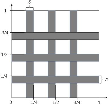
Figure 2.1: An example of $Q(j,\delta,d)$ with $j=2$ and $d=2$. It is the union of the white region in $[0,1]^{d}$.

Finally, for any function $f:\Omega\subseteq\mathbb{R}\to\mathbb{R}$, we will extend its definition to $\Omega^{d}$ by applying $f$ coordinate-wisely to ${\bm{x}}=(x_{1},\dots,x_{d})\in\Omega^{d}$, i.e. $f({\bm{x}}):=(f(x_{1}),\dots,f(x_{d}))$, without further notification.

In Table 2.1, we summarize a set of symbols that are used throughout this paper. Some of the notations will be introduced later.

Notation	Definition
$\mathbb{Z}^{d}_{j}$	$[0,2^{j}-1]^{d}\cap\mathbb{Z}^{d}$
$\,{\rm Bin}\,0.x_{1}x_{2}\cdots$	Binary representation of $x=\sum_{i=1}^{\infty}2^{-i}x_{i}$, $x_{i}\in\{0,1\}$
$Q(j,\delta,d)$	Approximately partition of $[0,1]^{d}$, Eq.(2.2)
$\mathcal{N}\mathcal{N}(N,L)$	Function class of neural networks with width $N$ and depth $L$
$\mathcal{S}_{j}(\varphi,M)$	Dilated shift-invariant space generated by $\varphi$, Eq.(2.4)
$\mathcal{E}(f,\mathcal{H};\mathcal{B})$	Approximation error of $f$ from $\mathcal{H}$ in the norm of $\mathcal{B}$, Eq.(2.5)
$m_{j}:[0,1)\to\mathbb{Z}_{j}$	$m_{j}(x)=\lfloor 2^{j}x\rfloor$, Lemma 3.1
$r_{j}:[0,1)\to[0,1)$	$r_{j}(x)=2^{j}x-m_{j}(x)$, Lemma 3.1
$\mathbb{Z}^{d}_{\varphi}$	$\{{\bm{n}}\in\mathbb{Z}^{d}:\exists{\bm{x}}\in[0,1)^{d}\ s.t.\ \varphi({\bm{x}}-{\bm{n}})\neq 0\}$, Lemma 3.1
$C_{\varphi}$	$|\mathbb{Z}^{d}_{\varphi}|$, the cardinality of $\mathbb{Z}^{d}_{\varphi}$

Table 2.1: A list of notations used in this paper.

2.2 Neural networks

In this paper, we only consider feed-forward neural networks with ReLU activation function $\sigma(x):=\max\{0,x\}$. Let $2\leq L\in\mathbb{N}$ and $N_{0},\dots,N_{L}\in\mathbb{N}$. We say $\eta=(A^{(\ell)},{\bm{a}}^{(\ell)})_{\ell=1}^{L}$ is a network architecture, if $A^{(\ell)}\in\mathbb{R}^{N_{\ell}\times N_{\ell}-1}$, ${\bm{a}}^{(\ell)}\in\mathbb{R}^{N_{\ell}}$ and each entry of $A^{(\ell)}$ and ${\bm{a}}^{(\ell)}$ is in $\{0,1\}$. We say a function $f:\mathbb{R}^{N_{0}}\to\mathbb{R}^{N_{L}}$ can be implemented (or represented) by a neural network with architecture $\eta$ if it can be written in the form

$$f({\bm{x}})=T_{L}(\sigma(T_{L-1}(\cdots\sigma(T_{1}({\bm{x}}))\cdots))),$$

where $T_{\ell}({\bm{x}}):=(A^{(\ell)}\odot B^{(\ell)}){\bm{x}}+{\bm{a}}^{(\ell)}\odot{\bm{b}}^{(\ell)}$ is an affine transformation with $B^{(\ell)}\in\mathbb{R}^{N_{\ell}\times N_{\ell-1}}$ and ${\bm{b}}^{(\ell)}\in\mathbb{R}^{N_{\ell}}$, and $\odot$ is entry-wise product. $L$ is called the depth of neural network. The width is referred to $N=\max\{N_{1},\dots,N_{L-1}\}$. The number of parameters of the architecture $\eta$ is $W=\sum_{\ell=1}^{L}\|A^{(\ell)}\|_{\ell^{0}}+\|{\bm{a}}^{(\ell)}\|_{\ell^{0}}$ and the number of (hidden) neurons is $U=\sum_{\ell=1}^{L-1}N_{\ell}$.

We will mainly focus on fully connected neural networks, which we refer to the case that all entries of $A^{(\ell)}$ and ${\bm{a}}^{(\ell)}$ are ones. Hence, we have no restriction on the coefficients of the affine maps $T_{\ell}({\bm{x}}):=B^{(\ell)}{\bm{x}}+{\bm{b}}^{(\ell)}$. When the input dimension $N_{0}$ and output dimension $N_{L}$ are clear from contexts, we denote by $\mathcal{N}\mathcal{N}(N,L)$ the set of functions that can be represented by neural networks with width at most $N$ and depth at most $L$. The expression “a neural network $\phi$ with width $N$ and depth $L$” means $\phi\in\mathcal{N}\mathcal{N}(N,L)$.

2.3 Shift-invariant spaces

Let $\varphi:\mathbb{R}^{d}\to\mathbb{R}$ be a continuous function with compact support. The shift-invariant space $\mathcal{S}(\varphi)$ generated by $\varphi$ is the set of all finite linear combinations of the shifts of $\varphi$, i.e. liner combination of $\varphi(\cdot-{\bm{n}})$ with ${\bm{n}}\in\mathbb{Z}^{d}$. For each $j\geq 0$, the dilated shift-invariant space $\mathcal{S}_{j}(\varphi)$ is defined to be the dilation of $\mathcal{S}(\varphi)$ by $2^{j}$. That is, every function $g\in S_{j}(\varphi)$ is of the form

$$g({\bm{x}})=\sum_{{\bm{n}}\in\mathbb{Z}^{d}}c_{\bm{n}}\varphi(2^{j}{\bm{x}}-{\bm{n}}),$$ (2.3)

where $(c_{\bm{n}})_{{\bm{n}}\in\mathbb{Z}^{d}}$ is zero except for finitely many ${\bm{n}}$. Note that the space $\mathcal{S}_{j}(\varphi)$ is invariant under the translations $T_{2^{-j}{\bm{m}}}g({\bm{x}}):=g({\bm{x}}-2^{-j}{\bm{m}})$ with ${\bm{m}}\in\mathbb{Z}^{d}$. For any $M>0$, we denote

$$\mathcal{S}_{j}(\varphi,M):=\left\{\sum_{{\bm{n}}\in\mathbb{Z}^{d}}c_{\bm{n}}\varphi(2^{j}{\bm{x}}-{\bm{n}})\in S_{j}(\varphi):|c_{\bm{n}}|<M\text{ for any }{\bm{n}}\in\mathbb{Z}^{d}\right\}.$$ (2.4)

2.4 Sobolev spaces and Besov spaces

For $1\leq p\leq\infty$, the $p$-norm of $L^{p}(\mathbb{R}^{d})$ is denoted by $\|\cdot\|_{p}$ for convenience. Let $k\in\mathbb{N}$, the Sobolev space $W^{k,p}(\mathbb{R}^{d})$ is the set of functions $f\in L^{p}(\mathbb{R}^{d})$ which have finite Sobolev norm

$$\|f\|_{W^{k,p}}:=\left(\sum_{\|\bm{\alpha}\|_{\ell^{1}}\leq k}\|D^{\bm{\alpha}}f\|^{p}_{p}\right)^{1/p},$$

where $D^{\bm{\alpha}}$ is the weak derivative of order $\bm{\alpha}$. There are several ways to generalize the definition of Sobolev norms to non-integer regularity. Here, we introduce the Besov spaces. Let us denote the difference operator by $\Delta_{\bm{y}}f({\bm{x}}):=f({\bm{x}}+{\bm{y}})-f({\bm{x}})$ for any ${\bm{x}},{\bm{y}}\in\mathbb{R}^{d}$. Then, for any positive integer $m$, the $m$-th modulus of smoothness of a function $f\in L^{p}(\mathbb{R}^{d})$ is defined by

$$\omega_{m}(f,h)_{p}:=\sup_{\|{\bm{y}}\|_{\ell^{2}}\leq h}\|\Delta_{\bm{y}}^{m}(f)\|_{p},\quad h\geq 0,$$

where

$$\Delta_{\bm{y}}^{m}(f)({\bm{x}}):=\sum_{j=0}^{m}\binom{m}{j}(-1)^{m-j}f({\bm{x}}+j{\bm{y}}).$$

For $\mu>0$ and $1\leq p,q\leq\infty$, the Besov space $B^{\mu}_{p,q}(\mathbb{R}^{d})$ is the collection of functions $f\in L^{p}(\mathbb{R}^{d})$ that have finite semi-norm $|f|_{B^{\mu}_{p,q}}<\infty$, where the semi-norm is defined as

$$|f|_{B^{\mu}_{p,q}}:=\left\{\begin{aligned} &\left(\int_{0}^{\infty}\left|\frac{\omega_{m}(f,t)_{p}}{t^{\mu}}\right|^{q}\frac{dt}{t}\right)^{1/q},\quad&&1\leq q<\infty,\\ &\sup_{t>0}\frac{\omega_{m}(f,t)_{p}}{t^{\mu}},\quad&&q=\infty,\end{aligned}\right.$$

where $m$ is an integer larger than $\mu$. The norm for $B^{\mu}_{p,q}$ is

$$\|f\|_{B^{\mu}_{p,q}}:=\|f\|_{p}+|f|_{B^{\mu}_{p,q}}.$$

Note that for $k\in\mathbb{N}$, we have the embedding $B^{k}_{p,1}\hookrightarrow W^{k,p}\hookrightarrow B^{k}_{p,\infty}$ and $B^{k}_{2,2}=W^{k,2}$. A general discussion of Sobolev spaces and Besov spaces can be found in DeVore and Lorentz (1993).

2.5 Approximation

Let $\mathcal{B}$ be a normed space and $f\in\mathcal{B}$, we denote the approximation error of $f$ from a set $\mathcal{H}\subseteq\mathcal{B}$ under the norm of $\mathcal{B}$ by

$$\mathcal{E}(f,\mathcal{H};\mathcal{B}):=\inf_{h\in\mathcal{H}}\|f-h\|_{\mathcal{B}}.$$ (2.5)

The approximation error of a set $\mathcal{F}\subseteq\mathcal{B}$ is the supremum approximation error of each function $f\in\mathcal{F}$, i.e.

$$\mathcal{E}(\mathcal{F},\mathcal{H};\mathcal{B}):=\sup_{f\in\mathcal{F}}\mathcal{E}(f,\mathcal{H};\mathcal{B})=\sup_{f\in\mathcal{F}}\inf_{h\in\mathcal{H}}\|f-h\|_{\mathcal{B}}.$$

Let $f\in\mathcal{B}$ and $\mathcal{G},\mathcal{H}\subseteq\mathcal{B}$, then for any $g\in\mathcal{G}$,

$$\mathcal{E}(f,\mathcal{H};\mathcal{B})=\inf_{h\in\mathcal{H}}\|f-h\|_{\mathcal{B}}\leq\|f-g\|_{\mathcal{B}}+\inf_{h\in\mathcal{H}}\|g-h\|_{\mathcal{B}}\leq\|f-g\|_{\mathcal{B}}+\mathcal{E}(\mathcal{G},\mathcal{H};\mathcal{B}).$$

By taking infimum over $g\in\mathcal{G}$, we get the “triangle inequality” for approximation error:

$$\mathcal{E}(f,\mathcal{H};\mathcal{B})\leq\mathcal{E}(f,\mathcal{G};\mathcal{B})+\mathcal{E}(\mathcal{G},\mathcal{H};\mathcal{B}).$$

Since we will mainly characterize the approximation error by width and depth of neural networks (or by number of neurons), we define the approximation order as follows.

Definition 2.1 (Order).

We say that the approximation order (by neural networks) of a function $\varphi:\mathbb{R}^{d}\to\mathbb{R}$ is at least $\alpha>0$ if

$$\mathcal{E}(\varphi,\mathcal{N}\mathcal{N}(N,L);L^{\infty}(\mathbb{R}^{d}))=\mathcal{O}((NL)^{-\alpha}).$$

More precisely, this definition means that there exist constants $C,M>0$ such that for any positive integers $N,L\geq M$, there exists a ReLU network $\phi$ with width $N$ and depth $L$ such that

$$\|\varphi-\phi\|_{\infty}\leq C(NL)^{-\alpha}.$$

3 Approximation in shift-invariant spaces

Let $\varphi:\mathbb{R}^{d}\to\mathbb{R}$ be a continuous function with compact support. We consider the question that how well deep neural networks can express functions in the shift-invariant space $\mathcal{S}_{j}(\varphi,M)$ generated by $\varphi$. More precisely, we want to estimate the size of network that is sufficient to approximate any function $g\in\mathcal{S}_{j}(\varphi,M)$ on $(0,1)^{d}$ with given accuracy.

Our estimation is based on a special representation of the function $g\in\mathcal{S}_{j}(\varphi,M)$.

Lemma 3.1.

For ${\bm{x}}\in[0,1)^{d}$, any $g\in\mathcal{S}_{j}(\varphi,M)$ can be written as

$$g({\bm{x}})=\sum_{{\bm{k}}\in\mathbb{Z}^{d}_{\varphi}}c_{m_{j}({\bm{x}})+{\bm{k}}}\varphi(r_{j}({\bm{x}})-{\bm{k}}),$$

where the coefficients $|c_{m_{j}({\bm{x}})+{\bm{k}}}|<M$, the functions $m_{j}:[0,1)\to\mathbb{Z}_{j}$ and $r_{j}:[0,1)\to[0,1)$ are defined by $m_{j}(x)=\lfloor 2^{j}x\rfloor$ and $r_{j}(x)=2^{j}x-m_{j}(x)$ and apply to ${\bm{x}}\in[0,1)^{d}$ coordinate-wisely, and

$$\mathbb{Z}^{d}_{\varphi}:=\{{\bm{n}}\in\mathbb{Z}^{d}:\exists{\bm{x}}\in[0,1)^{d}\ s.t.\ \varphi({\bm{x}}-{\bm{n}})\neq 0\}.$$

Proof.

Recall that we denote $\mathbb{Z}^{d}_{j}=[0,2^{j}-1]^{d}\cap\mathbb{Z}^{d}$ and notice that $\{[0,2^{-j})^{d}+2^{-j}{\bm{m}}\}_{{\bm{m}}\in\mathbb{Z}_{j}^{d}}$ is a partition of the cube $[0,1)^{d}$. If we denote the characteristic function of a set $A$ by $1_{A}$, i.e. $1_{A}({\bm{x}})=1$ if ${\bm{x}}\in A$ and $1_{A}({\bm{x}})=0$ otherwise, then for ${\bm{x}}\in[0,1)^{d}$,

$$\sum_{{\bm{m}}\in\mathbb{Z}_{j}^{d}}1_{[0,2^{-j})^{d}+2^{-j}{\bm{m}}}({\bm{x}})=1.$$

For any $g\in\mathcal{S}_{j}(\varphi,M)$ of the form (2.3), one has

$$g({\bm{x}}) =\sum_{{\bm{n}}\in\mathbb{Z}^{d}}c_{\bm{n}}\varphi(2^{j}{\bm{x}}-{\bm{n}})$$

$$=\sum_{{\bm{m}}\in\mathbb{Z}_{j}^{d}}\sum_{{\bm{n}}\in\mathbb{Z}^{d}}c_{{\bm{n}}}\varphi(2^{j}{\bm{x}}-{\bm{n}})\cdot 1_{[0,2^{-j})^{d}+2^{-j}{\bm{m}}}({\bm{x}})$$

$$=\sum_{{\bm{m}}\in\mathbb{Z}_{j}^{d}}\sum_{{\bm{k}}\in\mathbb{Z}^{d}_{\varphi}}c_{{\bm{m}}+{\bm{k}}}\varphi(2^{j}{\bm{x}}-{\bm{m}}-{\bm{k}})\cdot 1_{[0,2^{-j})^{d}+2^{-j}{\bm{m}}}({\bm{x}}).$$

To see the last equality, notice that for each ${\bm{m}}\in\mathbb{Z}^{d}_{j}$, ${\bm{x}}\in[0,2^{-j})^{d}+2^{-j}{\bm{m}}$ if and only if $2^{j}{\bm{x}}-{\bm{m}}\in[0,1)^{d}$. If we denote ${\bm{k}}:={\bm{n}}-{\bm{m}}$, then $\varphi(2^{j}{\bm{x}}-{\bm{n}})=\varphi(2^{j}{\bm{x}}-{\bm{m}}-{\bm{k}})$ is a nonzero function of ${\bm{x}}$ if and only if ${\bm{k}}\in\mathbb{Z}^{d}_{\varphi}$ by the definition of $\mathbb{Z}^{d}_{\varphi}$. Hence the last equality holds.

Observing that $1_{[0,2^{-j})^{d}+2^{-j}{\bm{m}}}({\bm{x}})\neq 0$ if and only if ${\bm{m}}=m_{j}({\bm{x}})$, we have

$$g({\bm{x}})=\sum_{{\bm{k}}\in\mathbb{Z}^{d}_{\varphi}}c_{m_{j}({\bm{x}})+{\bm{k}}}\varphi(2^{j}{\bm{x}}-m_{j}({\bm{x}})-{\bm{k}}).$$

Finally, using $r_{j}({\bm{x}})=2^{j}{\bm{x}}-m_{j}({\bm{x}})$, we get the desired representation. ∎

Notice that $m_{j}(x)$ and $r_{j}(x)$ are just the integer part and fractional part of $2^{j}x$. They can be represented in binary forms. Let the binary representation of $x\in[0,1)$ be

$$x=\sum_{l=1}^{\infty}2^{-l}x_{l}=\,{\rm Bin}\,0.x_{1}x_{2}\cdots,$$

with $x_{l}\in\{0,1\}$. Then, by straightforward calculation,

$$m_{j}(x) =2^{j-1}x_{1}+2^{j-2}x_{2}+\cdots+2^{0}x_{j},$$ (3.1)

$$r_{j}(x) =2^{j}x-m_{j}(x)=\,{\rm Bin}\,0.x_{j+1}x_{j+2}\cdots.$$

So $m_{j}(x)$ and $r_{j}(x)$ can be computed if we can extract the first $j$ bits of $x$, which can be done using the bit extraction technique (see section 6.1).

Now, suppose we can construct a network $\phi_{0}$ to approximate the generating function $\varphi$ with given accuracy: $\|\varphi-\phi_{0}\|_{\infty}\leq\epsilon$. According to Lemma 3.1, we can approximate $g\in\mathcal{S}_{j}(\varphi,M)$ by concatenating $C_{\varphi}:=|\mathbb{Z}^{d}_{\varphi}|$ sub-networks:

$$g({\bm{x}})\approx\sum_{{\bm{k}}\in\mathbb{Z}^{d}_{\varphi}}c_{m_{j}({\bm{x}})+{\bm{k}}}\phi_{0}(r_{j}({\bm{x}})-{\bm{k}}).$$

To approximate each term, we can first extract the location information ${\bm{x}}\mapsto(m_{j}({\bm{x}}),r_{j}({\bm{x}}))$ using bit extraction. Then, for fixed ${\bm{k}}$, the coefficient $c_{m_{j}({\bm{x}})+{\bm{k}}}=c_{\bm{k}}(m_{j}({\bm{x}}))$ can be regard as a function of $m_{j}({\bm{x}})\in\mathbb{Z}_{j}^{d}$. Therefore, approximating the coefficient function $c_{\bm{k}}(m_{j}({\bm{x}}))$ is equivalent to fit $\mathcal{O}(|\mathbb{Z}_{j}^{d}|)=\mathcal{O}(2^{jd})$ samples, which can be done using $\mathcal{O}(2^{jd/2})$ neurons by bit-extraction technique (see Lemma 6.7). Thus, we need $\mathcal{O}(C_{\varphi}2^{jd/2})$ neurons to approximate $g$ in general.

Alternative to use the representation in Lemma 3.1, one can approximate $g$ by computing each term in (2.3) directly. This straightforward approach is used in Shaham et al. (2018), which constructs a wavelet series using a network of depth 4. Similar ideas appear in Yarotsky (2017); Petersen and Voigtlaender (2018); Elbrächter et al. (2021); Bölcskei et al. (2019). However, the size of neural networks constructed in this approach is larger than ours. One can show that, for ${\bm{x}}\in[0,1)^{d}$, the non-zero terms in the summation (2.3) are those for ${\bm{n}}\in\mathbb{Z}^{d}_{\varphi}+\mathbb{Z}^{d}_{j}$. Since each term is approximated by one sub-network, it requires totally $\mathcal{O}(C_{\varphi}2^{jd})$ sub-networks to approximate $g$ in general, which needs $\mathcal{O}(C_{\varphi}2^{jd})$ neurons.

For our construction of ReLU neural networks, the main difficulty is that the function $m_{j}$ is discontinuous, hence it can not be implemented by ReLU neural networks exactly. To overcome this, we first consider the approximation on $Q(j,\delta,d)$ defined in (2.2), where we can compute $m_{j}({\bm{x}})$ and $r_{j}({\bm{x}})$ using the binary representation of ${\bm{x}}$ and the bit extraction technique. Combined with the data fitting results of deep neural networks, we can then approximate $g$ on $Q(j,\delta,d)$ to any prescribed accuracy. The approximation result is summarized in the following theorem. It also gives explicitly the required size of the network in our construction. The detailed proof is deferred to section 6.

Theorem 3.2 (Approximation on $Q(j,\delta,d)$).

Given any $j\in\mathbb{N}$, $0<\delta<2^{-j}$ and $0<\epsilon<1$. Assume that $\varphi:\mathbb{R}^{d}\to\mathbb{R}$ is a continuous function with compact support and there exists a ReLU network $\phi_{0}$ with width $N_{\varphi}(\epsilon)$ and depth $L_{\varphi}(\epsilon)$ such that

$$\|\varphi-\phi_{0}\|_{\infty}\leq\|\varphi\|_{\infty}\epsilon.$$

Then for any $g\in\mathcal{S}_{j}(\varphi,M)$ and any $r,s,\tilde{r},\tilde{s}\in\mathbb{N}$ with $2(s+r)\geq dj$ and $\tilde{r}\tilde{s}\geq\lceil\log_{2}(1/\epsilon)\rceil+1$, there exists a ReLU network $\phi$ with width $C_{\varphi}(\max\{7d\tilde{r}2^{r},N_{\varphi}(\epsilon)\}+4d)$ and depth $14\tilde{s}2^{s}+L_{\varphi}(\epsilon)$ such that for any ${\bm{x}}\in Q(j,\delta,d)$,

$$|g({\bm{x}})-\phi({\bm{x}})|\leq 3C_{\varphi}M\|\varphi\|_{\infty}\epsilon.$$

To estimate the uniform approximation error, we will use the “horizontal shift” method proposed in Lu et al. (2020). The key idea is to approximate the target function on several domain, which have similar structure as $Q(j,\delta,d)$, that cover $[0,1]^{d}$ and then use the middle function $\,{\rm mid}\,(\cdot,\cdot,\cdot)$ to compute the final approximation, where $\,{\rm mid}\,(\cdot,\cdot,\cdot)$ is a function that return the middle value of the three inputs. Specifically, for each ${\bm{x}}\in[0,1]^{d}$, we compute three approximation of $g({\bm{x}})$. If at least two of these approximation have the desired accuracy, then their middle value also has the same accuracy. Using this fact, we get the following uniform approximation result.

Theorem 3.3 (Uniform approximation).

Under the assumption of Theorem 3.2, for any $g\in\mathcal{S}_{j}(\varphi,M)$ and any $r,s,\tilde{r},\tilde{s}\in\mathbb{N}$ with $2(s+r)\geq dj$ and $\tilde{r}\tilde{s}\geq\lceil\log_{2}(1/\epsilon)\rceil+1$, there exists a ReLU network $\phi$ with width $3^{d}\cdot 2C_{\varphi}(\max\{7d\tilde{r}2^{r},N_{\varphi}(\epsilon)\}+4d)$ and depth $14\tilde{s}2^{s}+L_{\varphi}(\epsilon)+2d$ such that

$$\|g-\phi\|_{L^{\infty}([0,1]^{d})}\leq 6C_{\varphi}M\|\varphi\|_{\infty}\epsilon.$$

Before preceding, we would like to give a remark and a corollary on these theorems.

Remark 3.4.

Guaranteed by universality theorems (Pinkus, 1999), there always exist neural networks that approximate $\varphi$ arbitrarily well. But the required width $N_{\varphi}(\epsilon)$ and depth $L_{\varphi}(\epsilon)$ are generally unknown, except for certain types of $\varphi$, such as piecewise polynomials.

Corollary 3.5.

Suppose $1\leq p\leq\infty$ and $\varphi$ satisfies the assumption of Theorem 3.2. For any $g\in\mathcal{S}_{j}(\varphi,M)$, we have the following $L^{p}$ approximation result: for any $\epsilon>0$ and any $r,s\in\mathbb{N}$ with $2(s+r)\geq dj$, there exists a ReLU network with width $\mathcal{O}(2^{r}\log_{2}(1/\epsilon)+N_{\varphi}(\epsilon))$ and depth $\mathcal{O}(2^{s}\log_{2}(1/\epsilon)+L_{\varphi}(\epsilon))$ such that

$$\|g-\phi\|_{L^{p}([0,1]^{d})}\leq\epsilon.$$

Proof.

The $L^{p}$-estimations for $1\leq p<\infty$ can be obtained directly from the uniform approximation in Theorem 3.3 or by choosing sufficiently small $\delta$ in Theorem 3.2 so that the measure of $[0,1]^{d}\setminus Q(j,\delta,d)$ is small enough. We can choose $\tilde{r},\tilde{s}\asymp\log_{2}(1/\epsilon)$ in these theorems to get the desired approximation result. ∎

Besides the importance and interest in its own right, the dilated shift-invariant spaces are closely related to many other types of functions. These connections can be utilized to extend the above estimations of approximation error to other functions. Specifically, let $f$ be a function that is approximated by neural networks $\mathcal{N}\mathcal{N}(N,L)$ on the compact set $[0,1]^{d}$, we aim to estimate

$$\mathcal{E}(f,\mathcal{N}\mathcal{N}(N,L);L^{p}([0,1]^{d}))=\inf_{\phi\in\mathcal{N}\mathcal{N}(N,L)}\|f-\phi\|_{L^{p}([0,1]^{d})},$$

for some $1\leq p\leq\infty$. For an arbitrary $f$, it is in general difficult to directly construct a neural network with given size that achieves the minimal error rate. A more feasible way is to choose some function class $\mathcal{G}$ as a bridge, and estimate the approximation error by the triangle inequality

$$\mathcal{E}(f,\mathcal{N}\mathcal{N}(N,L);L^{p}([0,1]^{d}))\leq\mathcal{E}(f,\mathcal{G};L^{p}([0,1]^{d}))+\mathcal{E}(\mathcal{G},\mathcal{N}\mathcal{N}(N,L);L^{p}([0,1]^{d})).$$

Here, we choose $\mathcal{G}$ to be a dilated shift-invariant space $\mathcal{S}_{j}(\varphi,M)$. The success of this approach depends on how well we can estimate the two terms on the right hand side of the triangle inequality. The first term is well studied in the approximation theory of shift-invariant spaces, see (De Boor et al., 1994; Jia and Lei, 1993; Lei et al., 1997; Kyriazis, 1995; Jia, 2004, 2010). The second term $\mathcal{E}(\mathcal{S}_{j}(\varphi,M),\mathcal{N}\mathcal{N}(N,L);L^{p}([0,1]^{d}))$ can be estimated using our results, i.e. Theorems 3.2 and 3.3. Generally, we have the following.

Theorem 3.6.

Let $\varphi:\mathbb{R}^{d}\to\mathbb{R}$ be a continuous function with compact support and let its approximation order be at least $\alpha$. Then for any $f:\mathbb{R}^{d}\to\mathbb{R}$ satisfying

$$\mathcal{E}(f,\mathcal{S}_{j}(\varphi,M);L^{p}([0,1]^{d}))=\mathcal{O}(2^{-\beta j}),$$

for some $M>0$, $1\leq p\leq\infty$ and $\beta>0$, we have

$$\mathcal{E}(f,\mathcal{N}\mathcal{N}(N,L);L^{p}([0,1]^{d}))=\mathcal{O}\left(\max\left\{(NL)^{-\alpha},(NL/(\log_{2}N\log_{2}L))^{-2\beta/d}\right\}\right).$$

Proof.

Denote $\epsilon=2^{-\beta j}$. By assumption, there exists $g\in\mathcal{S}_{j}(\varphi,M)$ such that

$$\|f-g\|_{L^{p}([0,1]^{d})}=\mathcal{O}(2^{-\beta j})=\mathcal{O}(\epsilon).$$

Let $r,s$ be positive integers that satisfy $2(r+s)\geq dj$. Since the approximation order of $\varphi$ is $\alpha$, there exists a network $\phi_{0}$ with width $N_{\varphi}\asymp 2^{2\beta r/(d\alpha)}$ and depth $L_{\varphi}\asymp 2^{2\beta s/(d\alpha)}$ such that

$$\|\varphi-\phi_{0}\|_{\infty}=\mathcal{O}((N_{\varphi}L_{\varphi})^{-\alpha})=\mathcal{O}(2^{-2\beta(r+s)/d})=\mathcal{O}(2^{-\beta j})=\mathcal{O}(\epsilon).$$

Observe that $2rs=rs+rs\geq r+s\geq dj/2\asymp\log_{2}1/\epsilon$, we can choose $\tilde{r}\asymp r$ and $\tilde{s}\asymp s$ in Theorems 3.2 and 3.3. Thus, there exists a network $\phi$ with width $N=\mathcal{O}(r2^{r}+2^{2\beta r/(d\alpha)})$ and depth $L=\mathcal{O}(s2^{s}+2^{2\beta s/(d\alpha)})$ such that

$$\|g-\phi\|_{L^{p}([0,1]^{d})}=\mathcal{O}(\epsilon).$$

Now we consider two cases:

Case I: if $\alpha\geq 2\beta/d$, then we have $N=\mathcal{O}(r2^{r})$ and $L=\mathcal{O}(s2^{s})$. Hence, for any $\tilde{N}=2^{r}$ and $\tilde{L}=2^{s}$, there exists a network $\phi$ with width $N\asymp\tilde{N}\log_{2}\tilde{N}$ and depth $L\asymp\tilde{L}\log_{2}\tilde{L}$ such that

$$\|f-\phi\|_{L^{p}([0,1]^{d})}=\mathcal{O}(\epsilon)=\mathcal{O}(2^{-\beta j})=\mathcal{O}((\tilde{N}\tilde{L})^{-2\beta/d})=\mathcal{O}((NL/(\log_{2}N\log_{2}L))^{-2\beta/d}).$$

Case II: if $\alpha<2\beta/d$, then we have $L=\mathcal{O}(2^{2\beta s/(d\alpha)})$ and $N=\mathcal{O}(2^{2\beta r/(d\alpha)})$. Hence, there exists a network $\phi$ with width $N\asymp 2^{2\beta r/(d\alpha)}$ and depth $L\asymp 2^{2\beta s/(d\alpha)}$ such that

$$\|f-\phi\|_{L^{p}([0,1]^{d})}=\mathcal{O}(\epsilon)=\mathcal{O}(2^{-\beta j})=\mathcal{O}((NL)^{-\alpha}).$$

Combining these two cases, we finish the proof. ∎

Roughly speaking, Theorem 3.6 indicates that the approximation order of $f$ is at least $\min\{\alpha,2\beta/d\}$ (up to some log factors), where $\alpha$ is the approximation order of $\varphi$ by neural networks and $\beta$ is the order of the linear approximation by $S_{j}(\varphi,M)$. In practice, we need to choose the function $\varphi$ with large order $\alpha$, that is, the function that can be well approximated by deep neural networks. In particular, the approximation error $\mathcal{E}(f,\mathcal{S}_{j}(\varphi,M);L^{p}([0,1]^{d}))$ can be estimated for $f$ in many classical function spaces, such as Sobolev spaces and Besov spaces. It will be clear in the next section that deep neural networks can approximate piecewise polynomials with exponential convergence rate, which leads to an asymptotically optimal bound for Sobolev spaces.

4 Application to Sobolev spaces and Besov spaces

In this section, we apply our results to the approximation in Sobolev space $W^{\mu,p}$ and Besov space $B^{\mu}_{p,q}$. Similar approximation bounds can be obtained for the Triebel–Lizorkin spaces $F^{\mu}_{p,q}$ using the same method. The approximation rates of these spaces from shift-invariant spaces have been studied extensively in the literature (De Boor et al., 1994; Jia and Lei, 1993; Lei et al., 1997; Kyriazis, 1995; Jia, 2004, 2010). Roughly speaking, when $\varphi$ satisfies the Strang–Fix condition of order $k$, then the shift-invariant space $\mathcal{S}_{j}(\varphi)$ locally contains all polynomials of order $k-1$ and the approximation error of $f\in W^{\mu,p}$ or $f\in B^{\mu}_{p,q}$ is $\mathcal{O}(2^{-\mu j})$ if the regularity $\mu<k$.

4.1 Approximation of Sobolev functions and Besov functions

We follow the quasi-projection scheme in Jia (2004, 2010). Suppose $1\leq p\leq\infty$ and $1/p+1/\tilde{p}=1$. Let $\varphi\in L^{p}(\mathbb{R}^{d})$ and $\tilde{\varphi}\in L^{\tilde{p}}$ be compactly supported functions, and, for each ${\bm{n}}\in\mathbb{Z}^{d}$, $\varphi_{\bm{n}}=\varphi(\cdot-{\bm{n}})$ and $\tilde{\varphi}_{\bm{n}}=\tilde{\varphi}(\cdot-{\bm{n}})$. Then we can define the quasi-projection operator

$$\mathcal{Q}f:=\sum_{{\bm{n}}\in\mathbb{Z}^{d}}\langle f,\tilde{\varphi}_{\bm{n}}\rangle\varphi_{\bm{n}},\quad f\in L^{p}(\mathbb{R}^{d}).$$

For $h>0$, the dilated quasi-projection operator is defined as

$$\mathcal{Q}_{h}f({\bm{x}})=\sum_{{\bm{n}}\in\mathbb{Z}^{d}}\langle f,h^{-d/\tilde{p}}\tilde{\varphi}_{\bm{n}}(\cdot/h)\rangle h^{-d/p}\varphi_{\bm{n}}({\bm{x}}/h),\quad{\bm{x}}\in\mathbb{R}^{d}.$$

Notice that if $h=2^{-j}$, $\mathcal{Q}_{h}f$ is in the completion of the shift-invariant space $\mathcal{S}_{j}(\varphi)$.

If $\varphi$ satisfies the Strang-Fix condition of order $k$:

$$\hat{\varphi}(0)\neq 0,\ \mbox{and }D^{\bm{\alpha}}\hat{\varphi}(2{\bm{n}}\pi)=0,\quad{\bm{n}}\in\mathbb{Z}^{d}\setminus\{0\},|\bm{\alpha}|<k,$$

where $\hat{\varphi}(\bm{\omega})=\int\varphi({\bm{x}})e^{-i{\bm{x}}\cdot\bm{\omega}}d{\bm{x}}$ is the Fourier transform of $\varphi$, then we can choose $\tilde{\varphi}$ such that the quasi-projection operator $\mathcal{Q}$ has the polynomial reproduction property: $\mathcal{Q}g=g$ for all polynomials $g$ with order $k-1$. The approximation error $f-\mathcal{Q}f$ has been estimate in Jia (2004, 2010) when the quasi-projection operator has the polynomial reproduction property. The following lemma is a consequence of the results.

Lemma 4.1.

Let $k\in\mathbb{N}$, $0<\mu<k$, $1\leq p,q\leq\infty$ and $\mathcal{F}$ be either the Sobolev space $W^{\mu,p}$ or the Besov space $B^{\mu}_{p,q}$. If $\varphi$ satisfies the Strang-Fix condition of order $k$, then there exists $\tilde{\varphi}$ and a constant $C>0$ such that for any $f\in\mathcal{F}$,

$$\|f-\mathcal{Q}_{2^{-j}}f\|_{p}\leq C2^{-\mu j}\|f\|_{\mathcal{F}}.$$

A fundamental example that satisfies the Strang-Fix condition is the multivariate B-splines of order $k\geq 2$ defined by

$$\mathcal{N}_{k}^{d}({\bm{x}}):=\prod_{i=1}^{d}\mathcal{N}_{k}(x_{i}),\quad{\bm{x}}=(x_{1},\dots,x_{d})\in\mathbb{R}^{d},$$

where the univariate cardinal B-spline $\mathcal{N}_{k}$ of order $k$ is given by

$$\mathcal{N}_{k}(x):=\frac{1}{(k-1)!}\sum_{l=0}^{k}(-1)^{l}\binom{k}{l}\sigma(x-l)^{k-1},\quad x\in\mathbb{R}.$$

It is well known that $\|\mathcal{N}_{k}\|_{\infty}=1$ and the support of $\mathcal{N}_{k}$ is $[0,k]$. Alternatively, the B-spline $\mathcal{N}_{k}$ can be defined inductively by the convolution $\mathcal{N}_{k}=\mathcal{N}_{k-1}*\mathcal{N}_{1}$ where $\mathcal{N}_{1}(x)=1$ for $x\in[0,1]$ and $\mathcal{N}_{1}(x)=0$ otherwise. Hence, the Fourier transform of $\mathcal{N}_{k}$ is $\widehat{\mathcal{N}_{k}}(\omega)=\left(\frac{1-e^{-i\omega}}{i\omega}\right)^{k}$. The relation of B-splines approximation and Besov spaces is discussed in DeVore and Popov (1988).

The following lemma gives the approximation order of $\mathcal{N}_{k}$ by deep neural networks.

Lemma 4.2.

For any $N,L,k\in\mathbb{N}$ with $k\geq 3$, there exists a ReLU network $\phi$ with width $d(k+1)(9(N+1)+k)$ and depth $7(k^{2}+d^{2})L$ such that

$$\|\mathcal{N}_{k}^{d}-\phi\|_{\infty}\leq 9d\frac{(2k+2)^{k}}{(k-1)!}(N+1)^{-7(k-1)L}+9(d-1)(N+1)^{-7dL}.$$

Given any $k\geq 3$, this lemma implies that

$$\mathcal{E}(\mathcal{N}_{k}^{d},\mathcal{N}\mathcal{N}(N,L);L^{\infty}(\mathbb{R}^{d}))=\mathcal{O}(N^{-\mathcal{O}(L)}).$$

Hence, the approximation order of $\mathcal{N}_{k}^{d}$ can be chosen to be any $\alpha>0$. Theorem 3.6 and Lemma 4.1 imply that the approximation error of any $f\in W^{\mu,p}$ or $f\in B^{\mu}_{p,q}$ is

$$\mathcal{O}((NL/(\log_{2}N\log_{2}L))^{-2\mu/d}).$$

A more detailed analysis reveals that this bound is uniform for the unit ball of the spaces. We summarize the results in the following theorem.

Theorem 4.3.

Let $\mathcal{F}$ be either the unit ball of Sobolev space $W^{\mu,p}$ or the Besov space $B^{\mu}_{p,q}$. We have the following estimate of the approximation error

$$\mathcal{E}(\mathcal{F},\mathcal{N}\mathcal{N}(N,L);L^{p}([0,1]^{d}))=\mathcal{O}\left((NL/(\log_{2}N\log_{2}L))^{-2\mu/d}\right).$$

Proof.

Let $f\in\mathcal{F}$ and $k>\mu$, then by Lemma 4.1, $\|f-\mathcal{Q}_{2^{-j}}f\|_{p}\leq C2^{-\mu j}\|f\|_{\mathcal{F}}$, where $\mathcal{Q}_{2^{-j}}f=\sum_{{\bm{n}}\in\mathbb{Z}^{d}}c_{\bm{n}}(f)\mathcal{N}_{k}^{d}(2^{j}\cdot-{\bm{n}})$ is a B-spline series. It can be shown that the coefficients of a B-spline series is bounded by the $L^{p}$ norm of the series: $|c_{\bm{n}}(f)|\leq C2^{dj/p}\|\mathcal{Q}_{2^{-j}}(f)\|_{p}$ (See, for example, (DeVore and Lorentz, 1993, Chapter 5.4) and (DeVore and Popov, 1988, Lemma 4.1)). Hence, $|c_{\bm{n}}(f)|\leq C2^{dj/p}\|f\|_{\mathcal{F}}\leq C2^{dj/p}$, which implies $\mathcal{Q}_{2^{-j}}f\in\mathcal{S}_{j}(\mathcal{N}_{k}^{d},M)$ with $M\leq C2^{dj/p}$.

Let $r,s\in\mathbb{N}$ satisfy $2(r+s)\geq dj$, denote $\widetilde{N}=2^{r}$, $\widetilde{L}=2^{s}$ and choose $\epsilon=2^{-\mu j-dj/p}$. By Lemma 4.2, if $N,L$ are sufficiently large, $\mathcal{E}(\mathcal{N}_{k}^{d},\mathcal{N}\mathcal{N}(N,L),L^{\infty}(\mathbb{R}^{d}))\leq C_{k,d}N^{-7L}\leq C_{k,d}(NL)^{-\alpha}$, where we choose $\alpha=2+2\mu/d$. Thus, there exists a network $\phi_{0}$ with width $\mathcal{O}(\widetilde{N})$ and depth $\mathcal{O}(\widetilde{L})$ such that

$$\|\mathcal{N}_{k}^{d}-\phi_{0}\|_{\infty}\leq(\widetilde{N}\widetilde{L})^{-\alpha}\leq 2^{-dj\alpha/2}=2^{-\mu j-dj}\leq\epsilon.$$

Since $2rs=rs+rs\geq r+s\geq dj/2\asymp\log_{2}1/\epsilon$, we can choose $\tilde{r}\asymp r$ and $\tilde{s}\asymp s$ in Theorem 3.2 and Theorem 3.3. Therefore, since $\mathcal{Q}_{2^{-j}}f\in\mathcal{S}_{j}(\mathcal{N}_{k}^{d},M)$, there exists a network $\phi$ with width $\mathcal{O}(\widetilde{N}\log_{2}\widetilde{N})$ and depth $\mathcal{O}(\widetilde{L}\log_{2}\widetilde{L})$ such that

$$\|\mathcal{Q}_{2^{-j}}f-\phi\|_{L^{p}([0,1]^{d})}\leq CM\epsilon\leq C2^{-\mu j}.$$

The triangle inequality gives

$$\|f-\phi\|_{L^{p}([0,1]^{d})}\leq\mathcal{O}(2^{-\mu j})=\mathcal{O}((\widetilde{N}\widetilde{L})^{-2\mu/d}).$$

Finally, let $N=\tilde{N}\log_{2}\tilde{N}$ and $L=\tilde{L}\log_{2}\tilde{L}$, we have

$$\mathcal{E}(f,\mathcal{N}\mathcal{N}(N,L);L^{p}([0,1]^{d}))=\mathcal{O}((\widetilde{N}\widetilde{L})^{-2\mu/d})=\mathcal{O}\left((NL/(\log_{2}N\log_{2}L))^{-2\mu/d}\right).$$

Since the bound is uniform for all $f\in\mathcal{F}$, we finish the proof. ∎

So far, we characterize the approximation error by the number of neurons $NL$, we can also estimate the error by the number of weights. To see this, let the width $N$ be sufficiently large and fixed, then the number of weights $W\asymp N^{2}L\asymp L$ and we have

$$\mathcal{E}(\mathcal{F},\mathcal{N}\mathcal{N}(N,L);L^{p}([0,1]^{d}))=\mathcal{O}\left((W/\log_{2}W)^{-2\mu/d}\right).$$

Note that similar bounds have been obtained in Yarotsky and Zhevnerchuk (2020) and Lu et al. (2020) for Hölder spaces. The paper (Suzuki, 2019) also studies the approximation in Besov spaces, but they only get the bound $\mathcal{O}(W^{-\mu/d})$.

4.2 Optimality for Sobolev spaces

We consider the optimality of the upper bounds we have derived for the unit ball $\mathcal{F}$ of Sobolev spaces $W^{k,p}$. The main idea is to find the connection between the approximation accuracy and the Pseudo-dimension (or VC-dimension) of neural networks. Let us first introduce some results of Pseudo-dimension.

Definition 4.4 (Pseudo-dimension).

Let $\mathcal{H}$ be a class of real-valued functions defined on $\Omega$. The Pseudo-dimension of $\mathcal{H}$, denoted by $\,{\rm Pdim}\,(\mathcal{H})$, is the largest integer of $N$ for which there exist points $x_{1},\dots,x_{N}\in\Omega$ and constants $c_{1},\dots,c_{N}\in\mathbb{R}$ such that

$$|\{\,{\rm sgn}\,(h(x_{1})-c_{1}),\dots,\,{\rm sgn}\,(h(x_{N})-c_{N}):h\in\mathcal{H}\}|=2^{N}.$$

If no such finite value exists, $\,{\rm Pdim}\,(\mathcal{H})=\infty$.

There are some well-known upper bounds on Pseudo-dimension of deep ReLU networks in the literature (Anthony and Bartlett, 2009; Bartlett et al., 1999; Goldberg and Jerrum, 1995; Bartlett et al., 2019). We summarize two bounds in the following lemma.

Lemma 4.5.

Consider a network architecture $\eta$ with $W$ parameters, $U$ neurons and depth $L$. Let $\mathcal{H}_{\eta}$ be the set of functions that can be represented by such architecture with ReLU activation. Then there exists constants $C_{1},C_{2}>0$ such that

$$\,{\rm Pdim}\,(\mathcal{H}_{\eta})\leq C_{1}W^{2}\quad\mbox{and}\quad\,{\rm Pdim}\,(\mathcal{H}_{\eta})\leq C_{2}WL\log_{2}U.$$

Intuitively, if a function class $\mathcal{H}$ can approximate a function class $\mathcal{F}$ of high complexity with small precision, then $\mathcal{H}$ should also have high complexity. In other words, if we use a function class $\mathcal{H}$ with $\,{\rm Pdim}\,(\mathcal{H})\leq n$ to approximate a complex function class, we should be able to get a lower bound of the approximation error. Mathematically, we can define a nonlinear $n$-width using Pseudo-dimension: let $\mathcal{B}$ be a normed space and $\mathcal{F}\subseteq\mathcal{B}$, we define

$$\rho_{n}(\mathcal{F},\mathcal{B}):=\inf_{\mathcal{H}^{n}}\mathcal{E}(\mathcal{F},\mathcal{H}^{n};\mathcal{B})=\inf_{\mathcal{H}^{n}}\sup_{f\in\mathcal{F}}\inf_{h\in\mathcal{H}^{n}}\|f-h\|_{\mathcal{B}},$$

where $\mathcal{H}^{n}$ runs over all classes in $\mathcal{B}$ with $\,{\rm Pdim}\,(\mathcal{H}^{n})\leq n$.

We remark that the $n$-width $\rho_{n}$ is different from the famous continuous $n$-th width $\omega_{n}$ introduced by DeVore et al. (1989):

$$\omega_{n}(\mathcal{F},\mathcal{B}):=\inf_{{\bm{a}},M_{n}}\sup_{f\in\mathcal{F}}\|f-M_{n}({\bm{a}}(f))\|_{\mathcal{B}},$$

where ${\bm{a}}:\mathcal{F}\to\mathbb{R}^{n}$ is continuous and $M_{n}:\mathbb{R}^{n}\to\mathcal{F}$ is any mapping. In neural network approximation, ${\bm{a}}$ maps the target function $f\in\mathcal{F}$ to the parameters in neural network and $M_{n}$ is the realization mapping that associates the parameters to the function realized by neural network. Applying the results in DeVore et al. (1989), one can show that the approximation error of the unit ball of Sobolev space $W^{k,p}(\mathbb{R}^{d})$ is lower bounded by $cW^{-k/d}$, where $W$ is the number of parameters in the network, see (Yarotsky, 2017; Yarotsky and Zhevnerchuk, 2020). However, we have obtained an upper bound $\mathcal{O}((W/\log_{2}W)^{-2k/d})$ for these spaces. The inconsistency is because the parameters in our construction does not continuously depend on the target function and hence it does not satisfy the requirement in the $n$-width $\omega_{n}$. This implies that we can get better approximation order by taking advantage of the incontinuity.

The $n$-width $\rho_{n}$ was firstly introduced by Maiorov and Ratsaby (1999); Ratsaby and Maiorov (1997). They also gave upper and lower estimates of the $n$-width for Sobolev spaces. The following lemma is from Maiorov and Ratsaby (1999).

Lemma 4.6.

Let $\mathcal{F}$ be the unit ball of Sobolev space $W^{k,p}(\mathbb{R}^{d})$ and $1\leq p,q\leq\infty$, then

$$\rho_{n}(\mathcal{F},L^{q}([0,1]^{d}))\geq cn^{-k/d},$$

for some constant $c>0$ independent of $n$.

Combining Lemmas 4.5 and 4.6, we can give lower bound of the approximation error by ReLU neural networks. These lower bounds show that the upper bound in Theorem 4.3 is asymptotically optimal up to a logarithm factor.

Corollary 4.7.

Let $\mathcal{F}$ be the unit ball of Sobolev space $W^{k,p}(\mathbb{R}^{d})$ and $1\leq p,q\leq\infty$. For the function class $\mathcal{H}_{\eta}$ in Lemma 4.5, we have

$$\mathcal{E}(\mathcal{F},\mathcal{H}_{\eta};L^{q}([0,1]^{d}))\geq c_{1}W^{-2k/d}\quad\mbox{and}\quad\mathcal{E}(\mathcal{F},\mathcal{H}_{\eta};L^{q}([0,1]^{d}))\geq c_{2}(WL\log_{2}U)^{-k/d}.$$

for some constant $c_{1},c_{2}>0$. In particular, there exists $c>0$ such that

$$\mathcal{E}(\mathcal{F},\mathcal{N}\mathcal{N}(N,L);L^{q}([0,1]^{d}))\geq c(N^{2}L^{2}\log_{2}NL)^{-k/d}.$$

Proof.

We choose $n=\,{\rm Pdim}\,(\mathcal{H}_{\eta})$, then by the definition of the $n$-width $\rho_{n}(\mathcal{F},L^{q}([0,1]^{d}))$ and Lemma 4.6,

$$\mathcal{E}(\mathcal{F},\mathcal{H}_{\eta};L^{q}([0,1]^{d}))\geq\rho_{n}(\mathcal{F},L^{q}([0,1]^{d}))\geq c_{0}n^{-k/d}.$$

By lemma 4.5, we have $n=\,{\rm Pdim}\,(\mathcal{H}_{\eta})\leq C_{1}W^{2}$ and $n\leq C_{2}WL\log_{2}U$, which give the desired lower bounds for $\mathcal{E}(\mathcal{F},\mathcal{H}_{\eta};L^{q}([0,1]^{d}))$.

When $\mathcal{H}$ is the fully connected network $\mathcal{N}\mathcal{N}(N,L)$, we have $W=\mathcal{O}(N^{2}L)$ and $U=\mathcal{O}(NL)$. Hence,

$$\mathcal{E}(\mathcal{F},\mathcal{N}\mathcal{N}(N,L);L^{q}([0,1]^{d}))\geq c_{2}(WL\log_{2}U)^{-k/d}\geq c(N^{2}L^{2}\log_{2}NL)^{-k/d}.\qed$$

5 Discussion

In this paper, we study how well deep ReLU networks can approximate functions in dilated shift-invariant spaces. Our main theorems, Theorem 3.2 and 3.3, give upper bounds on the approximation error of these spaces. The results can be easily applied to wavelet, which is widely used in signal processing. As an illustration, we consider a multiresolution approximation $\{V_{j}\}_{j\in\mathbb{Z}}$ of $L^{2}(\mathbb{R})$, which satisfies $V_{j+1}\subseteq V_{j}$ for all $j\in\mathbb{Z}$. And let $\psi$ and $\varphi$ be the wavelet and the scaling function that generate an orthogonal basis (Mallat, 1999, Chapter 7). Denote $\varphi_{j,n}(x):=2^{-j/2}\varphi(2^{-j}x-n)$, then the orthogonal projection of $f\in L^{2}(\mathbb{R})$ over $V_{-j}$ is

$$P_{V_{-j}}f=\sum_{n=-\infty}^{+\infty}\langle f,\varphi_{-j,n}\rangle\varphi_{-j,n},$$

which has the same form of functions in the dilated shift-invariant space $\mathcal{S}_{j}(\varphi)$. Hence, Theorem 3.2 and 3.3 can be applied to derive approximation bound of the projection $P_{V_{-j}}f$. Alternatively, we can also approximate the wavelet decomposition

$$f=\sum_{j=-\infty}^{\infty}\sum_{n=-\infty}^{+\infty}\langle f,\psi_{j,n}\rangle\psi_{j,n},$$

using the approximation result for $\mathcal{S}_{j}(\psi)$.

The abstract approximation results for shift-invariant spaces can also be applied to study the approximation of classical smooth function spaces by deep neural networks, which has received much attention in recent years. When the approximation error is measured by the number parameters $W$, the seminal work of Yarotsky (2017) obtained approximation bound $\mathcal{O}(W^{-s/d})$ for the Sobolev spaces $W^{s,\infty}$, ignoring the logarithmic factors. The recent works (Yarotsky, 2018; Yarotsky and Zhevnerchuk, 2020) improved the upper bound to $\mathcal{O}(W^{-2s/d})$. In contrast, if the error is measured by the number of neurons $U\asymp NL$, Shen et al. (2020); Lu et al. (2020) showed the bound $\mathcal{O}\left(U^{-2s/d}\right)$ for smooth function class $C^{s}([0,1]^{d})$. All these results are derived through approximating local Taylor expansions by neural networks. In this paper, we take a multiresolution approximation point of view. By choosing the B-spline as the generating function $\varphi$ of the shift-invariant space $\mathcal{S}_{j}(\varphi)$, we can recover all the existing bounds and generalize them to the Besov spaces $B^{\mu}_{p,q}$. Our result improves the existing bounds for Besov spaces obtained by Suzuki (2019). We also prove lower bounds of the approximation error in $L^{p}$-norm ($1\leq p\leq\infty$), which show the optimality of the upper bounds. As far as we know, only $L^{\infty}$ lower bounds for neural network approximation are obtained in the literature.

Although the lower bounds in Corollary 4.7 are proved for ReLU networks, similar lower bounds can be derived for piecewise polynomial activation functions using the same argument and the upper bounds of Pseudo-dimension for such activation functions in Bartlett et al. (2019). However, for more complicated activation functions, this kind of lower bound may not exist. For example, Maiorov and Pinkus (1999) showed that there exists an analytic, strictly increasing, and sigmoidal activation function such that any continuous function on $[0,1]^{d}$ can be uniformly approximated to within any error by a neural network with width $6d+3$ and depth $3$. In other words, we can approximate any continuous function using a network of fixed finite size with this activation function. However, by Lemma 4.6, the function class generated by this network has infinite Pseudo-dimension, which is due to the high “complexity” of the activation function.

6 Proof of Theorem 3.2

Without loss of generality, we can assume that $M=1$ and $\|\varphi\|_{\infty}=1$. By Lemma 3.1, for ${\bm{x}}\in[0,1)^{d}$,

$$g({\bm{x}})=\sum_{{\bm{n}}\in\mathbb{Z}^{d}}c_{{\bm{n}}}\varphi(2^{j}{\bm{x}}-{\bm{n}})=\sum_{{\bm{k}}\in\mathbb{Z}^{d}_{\varphi}}c_{m_{j}({\bm{x}})+{\bm{k}}}\varphi(r_{j}({\bm{x}})-{\bm{k}}),$$

where $m_{j}$ and $r_{j}$ are applied coordinate-wisely to ${\bm{x}}=(x_{1},\dots,x_{d})\in[0,1)^{d}$ and

$$m_{j}(x_{i}) =2^{j-1}x_{i,1}+2^{j-2}x_{i,2}+\cdots+2^{0}x_{i,j},$$

$$r_{j}(x_{i}) =2^{j}x-m_{j}(x_{i})=\,{\rm Bin}\,0.x_{i,j+1}x_{i,j+2}\cdots,$$

if $x_{i}=\,{\rm Bin}\,0.x_{i,1}x_{i,2}\cdots$ is the binary representation of $x_{i}\in[0,1)$.

For any fixed ${\bm{k}}\in\mathbb{Z}^{d}$, we are going to construct a network that approximates the function

$${\bm{x}}\mapsto c_{m_{j}({\bm{x}})+{\bm{k}}}\varphi(r_{j}({\bm{x}})-{\bm{k}}),\quad{\bm{x}}\in Q(j,\delta,d).$$

We can summarize the result as follows.

Proposition 6.1.

For any fixed $j\in\mathbb{N}$ and ${\bm{k}}\in\mathbb{Z}^{d}$, there exists a network $\phi^{({\bm{k}})}$ with width $\max\{7d\tilde{r}2^{r},N_{\varphi}(\epsilon)\}+4d$ and depth $14\tilde{s}2^{s}+L_{\varphi}(\epsilon)$ such that for any ${\bm{x}}\in Q(j,\delta,d)$,

$$|c_{m_{j}({\bm{x}})+{\bm{k}}}\varphi(r_{j}({\bm{x}})-{\bm{k}})-\phi^{({\bm{k}})}({\bm{x}})|\leq 3\epsilon.$$

Assume that Proposition 6.1 is true. We can construct the desired function $\phi$ by

$$\phi({\bm{x}})=\sum_{{\bm{k}}\in\mathbb{Z}^{d}_{\varphi}}\phi^{({\bm{k}})}({\bm{x}}),$$

which can be computed by $C_{\varphi}$ parallel sub-networks $\phi^{({\bm{k}})}$. Since $\phi({\bm{x}})$ is a linear combination of $\phi^{({\bm{k}})}({\bm{x}})$, the required depth is $14\tilde{s}2^{s}+L_{\varphi}(\epsilon)$ and the required width is at most $C_{\varphi}(\max\{7d\tilde{r}2^{r},N_{\varphi}(\epsilon)\}+4d)$. The approximation error is

$$\left|\sum_{{\bm{n}}\in\mathbb{Z}^{d}}c_{{\bm{n}}}\varphi(2^{j}{\bm{x}}-{\bm{n}})-\phi({\bm{x}})\right|\leq\sum_{{\bm{k}}\in\mathbb{Z}^{d}_{\varphi}}|c_{m_{j}({\bm{x}})+{\bm{k}}}\varphi(r_{j}({\bm{x}})-{\bm{k}})-\phi^{({\bm{k}})}({\bm{x}})|\leq 3C_{\varphi}\epsilon.$$

It remains to prove Proposition 6.1. The key idea is as follows. Since $|c_{{\bm{m}}}|<1$, we let $b_{i}({\bm{m}})\in\{0,1\}$ be the $i$-bit of $c_{{\bm{m}}}/2+1/2\in[0,1)$. Thus, we have the binary representation

$$c_{{\bm{m}}}=\sum_{i=1}^{\infty}2^{1-i}b_{i}({\bm{m}})-1.$$ (6.1)

As a consequence, we have

$$c_{m_{j}({\bm{x}})+{\bm{k}}}\varphi(r_{j}({\bm{x}})-{\bm{k}})=\sum_{i=1}^{\infty}2^{1-i}b_{i}(m_{j}({\bm{x}})+{\bm{k}})\varphi(r_{j}({\bm{x}})-{\bm{k}})-\varphi(r_{j}({\bm{x}})-{\bm{k}}).$$

We will construct a neural network that approximates the truncation

$$\sum_{i=1}^{\lceil\log_{2}(1/\epsilon)\rceil+1}2^{1-i}b_{i}(m_{j}({\bm{x}})+{\bm{k}})\varphi(r_{j}({\bm{x}})-{\bm{k}})-\varphi(r_{j}({\bm{x}})-{\bm{k}}),\quad{\bm{x}}\in Q(j,\delta,d).$$

The construction can be divided into two parts:

1. For each $j\in\mathbb{N}$, construct a neural network to compute ${\bm{x}}\mapsto(m_{j}({\bm{x}}),r_{j}({\bm{x}}))$. This can be done by the bit extraction technique.

2. For each $i,j\in\mathbb{N}$, construct a neural network to compute ${\bm{m}}\in\mathbb{Z}_{j}^{d}\mapsto b_{i}({\bm{m}})$, which is equivalent to interpolate $2^{dj}$ samples $({\bm{m}},b_{i}({\bm{m}}))$.

We gather the necessary results in the following two subsections and give a proof of Proposition 6.1 in subsection 6.3.

6.1 Bit extraction

In order to compute $\,{\rm Bin}\,0.x_{1}x_{2}\cdots\mapsto(x_{1},\dots,x_{r})$, we need to use the bit extraction technique in Bartlett et al. (1999, 2019). Let us first introduce the basic lemma that extract $r$ bits using a shallow network.

Lemma 6.2.

Given $j\in\mathbb{N}$ and $0<\delta<2^{-j}$. For any positive integer $r\leq j$, there exists a network $\phi_{r}$ with width $2^{r+1}+1$ and depth $3$ such that

$$\phi_{r}(x)=(x_{1},\dots,x_{r},\,{\rm Bin}\,0.x_{r+1}x_{r+2}\cdots),\quad\forall x=\,{\rm Bin}\,0.x_{1}x_{2}\cdots\in Q(j,\delta,1).$$

Proof.

We follow the construction in Bartlett et al. (2019). For any $a\leq b$, observe that the function

$$f_{[a,b]}(x):=\sigma(1-\sigma(a/\delta-x/\delta))+\sigma(1-\sigma(x/\delta-b/\delta))-1$$

satisfies $f_{[a,b]}(x)=1$ for $x\in[a,b]$, and $f_{[a,b]}(x)=0$ for $x\notin(a-\delta,b+\delta)$, and $f_{[a,b]}(x)\in[0,1]$ for all $x$. So, we can use $f_{[a,b]}$ to approximate the indicator function of $[a,b]$, to precision $\delta$. Note that $f_{[a,b]}$ can be implemented by a ReLU network with width $2$ and depth $3$.

Since $x_{1},\dots,x_{r}$ can be computed by adding the corresponding indicator functions of $[k2^{-r},(k+1)2^{-r}]$, $0\leq k\leq 2^{r}-1$, we can compute $x_{1},\dots,x_{r}$ using $2^{r}$ parallel networks

$$f_{[1-2^{-r},1]},\quad f_{[k2^{-r},(k+1)2^{-r}-\delta]},\quad k=0,\dots,2^{r}-2.$$

Observe that

$$\,{\rm Bin}\,0.x_{r+1}x_{r+2}\cdots=2^{r}x-\sum_{i=1}^{r}2^{r-i}x_{i},$$

which is a linear combination of $x,x_{1},\dots,x_{r}$. There exists a network $\phi_{r}$ with width $2^{r+1}+1$ and depth $3$ such that $\phi_{r}(x)=(x_{1},\dots,x_{r},\,{\rm Bin}\,0.x_{r+1}x_{r+2}\cdots)$ for $x\in Q(j,\delta,1)$. (We can use one neuron in each hidden layer to ’remember’ the input $x$. Since $\phi_{r}(x)$ is a linear transform of $x$ and outputs of the parallel sub-networks, we do not need extra layer to compute summation.) ∎

Note that the function $\,{\rm Bin}\,0.x_{1}x_{2}\cdots\mapsto(x_{1},\dots,x_{r})$ is not continuous, while every ReLU network function is continuous. So, we cannot implement the bit extraction on the whole set $[0,1]$. This is why we restrict ourselves to $Q(j,\delta,1)$.

The next lemma is an extension of Lemma 6.2. It will be used to extract the location information $(m_{j}({\bm{x}}),r_{j}({\bm{x}}))$.

Lemma 6.3.

Given $r,j\in\mathbb{N}$ and $0<\delta<2^{-j}$. For any integer $k\leq j$, there exists a ReLU network $\phi$ with width $2^{r+1}+3$ and depth $2\lceil j/r\rceil+1$ such that

$$\phi(x)=\left(\sum_{i=1}^{k}2^{j-i}x_{i},\sum_{i=k+1}^{j}2^{j-i}x_{i},\,{\rm Bin}\,0.x_{j+1}x_{j+2}\cdots\right),\quad\forall x=\,{\rm Bin}\,0.x_{1}x_{2}\cdots\in Q(j,\delta,1).$$

Proof.

Without loss of generality, we can assume $r\leq j$. By Lemma 6.2, there exists a network $\phi_{r}$ with width $2^{r+1}+1$ and depth $3$ such that $\phi_{r}(x)=(x_{1},\dots,x_{r},\,{\rm Bin}\,0.x_{r+1}x_{r+2}\cdots)$. Observe that any summation $\sum_{i=1}^{k}2^{j-i}x_{i}$ and $\sum_{i=k+1}^{r}2^{j-i}x_{i}$ with $k\leq r$ are linear combinations of outputs of $\phi_{r}$. We can compute them by a network having the same size as $\phi_{r}$. If $k>r$, we compute $\sum_{i=1}^{r}2^{j-i}x_{i}$ as intermediate result. Then, by applying another $\phi_{r}$ to $\,{\rm Bin}\,0.x_{r+1}x_{r+2}\cdots$, we can extract the next $r$ bits $x_{r+1},\dots,x_{2r}$, and compute $\,{\rm Bin}\,0.x_{2r+1}x_{2r+2}\cdots$. Again, any summation $\sum_{i=1}^{k}2^{j-i}x_{i}$ and $\sum_{i=k+1}^{2r}2^{j-i}x_{i}$ with $k\leq 2r$ are linear combinations of the outputs. If $k>2r$, we compute $\sum_{i=1}^{2r}2^{j-i}x_{i}$ as intermediate result. Continuing this strategy, after we extract $\lfloor j/r\rfloor r$ bits, we can use $\phi_{j-\lfloor j/r\rfloor r}$ to extract the rest bits. Using this construction, we can compute the required function $\phi$ by a network with width at most $2^{r+1}+3$ and depth at most $2\lceil j/r\rceil+1$. (Two neurons in each hidden layer are used to ’remember’ the intermediate computation.) ∎

The following lemma shows how to extract a specific bit.

Lemma 6.4.

For any $r,K\in\mathbb{N}$ with $r\leq K$, there exists a ReLU network $\phi$ with width $2^{r+1}+3$ and depth $4\lceil K/r\rceil+1$ such that for any $x=\,{\rm Bin}\,0.x_{1}x_{2}\cdots x_{K}$ and positive integer $k\leq K$, we have $\phi(x,k)=x_{k}$.

Proof.

Let $\delta_{ki}=0$ if $k\neq i$ and $\delta_{ki}=1$ if $k=i$. Observe that

$$\delta_{ki}=\sigma(k-i+1)+\sigma(k-i-1)-2\sigma(k-i),$$

and $t_{1}t_{2}=\sigma(t_{1}+t_{2}-1)$ for any $t_{1},t_{2}\in\{0,1\}$. We have the expression

$$x_{k}=\sum_{i=1}^{K}\delta_{ki}x_{i}=\sum_{i=1}^{K}\sigma\left(\sigma(k-i+1)+\sigma(k-i-1)-2\sigma(k-i)+x_{i}-1\right).$$

By Lemma 6.2, there exists a ReLU network $\phi_{r}$ with width $2^{r+1}+1$ and depth $3$ such that $\phi_{r}(x)=(x_{1},\dots,x_{r},\,{\rm Bin}\,0.x_{r+1}x_{r+2}\cdots x_{K})$. Hence, the function

$$\tilde{\phi}_{r}(x,k)=\left(\,{\rm Bin}\,0.x_{r+1}x_{r+2}\cdots x_{K},k,\sum_{j=1}^{r}\delta_{kj}x_{j}\right)$$

is a network with width at most $\max\{2^{r+1},4r\}+3=2^{r+1}+3$ and depth $5$. Applying Lemma 6.2 to the first output $\,{\rm Bin}\,0.x_{r+1}x_{r+2}\cdots x_{K}$ and preserving the last output $(k,\sum_{j=1}^{r}\delta_{kj}x_{j})$, we can implement

$$\tilde{\phi}_{2r}(x,k)=\left(\,{\rm Bin}\,0.x_{2r+1}x_{2r+2}\cdots x_{K},k,\sum_{j=1}^{2r}\delta_{kj}x_{j}\right)$$

by a network with width $2^{r+1}+3$ and depth $9$. Using this construction iteratively, we can implement the required function $\phi(x,k)=x_{k}=\sum_{j=1}^{K}\delta_{kj}x_{j}$ by a network with width at most $2^{r+1}+3$ and depth $4\lceil K/r\rceil+1$. ∎

6.2 Interpolation

Given an arbitrary sample set $(x_{i},y_{i})$, $i=1,\dots,M$, we want to find a network $\phi$ with certain architecture to interpolate the data: $\phi(x_{i})=y_{i}$. This problem has been studied in many papers (Yun et al., 2019; Shen et al., 2019; Vershynin, 2020). Roughly speaking, the number of samples that a network can interpolate is in the order of the number of parameters.

The following lemma is a combination of Proposition 2.1 and 2,2 in Shen et al. (2019).

Lemma 6.5.

For any $N,L\in\mathbb{N}$, given $N^{2}L$ samples $(x_{i},y_{i})$, $i=1,\dots,N^{2}L$, with distinct $x_{i}\in\mathbb{R}^{d}$ and $y_{i}\geq 0$. There exists a ReLU network $\phi$ with width $4N+4$ and depth $L+2$ such that $\phi(x_{i})=y_{i}$ for $i=1,\dots,N^{2}L$.

We can also give an upper bound of the interpolation capacity of a given network architecture.

Proposition 6.6.

Let $\mathcal{H}=\{\phi_{\theta}:\mathbb{R}^{d_{in}}\to\mathbb{R}^{d_{out}}\}$ be the class of functions that can be represented by a ReLU network with architecture of $W$ parameters $\theta$. If for any $M$ samples $(x_{i},y_{i})$ with distinct $x_{i}\in\mathbb{R}^{d_{in}}$ and $y_{i}\in\mathbb{R}^{d_{out}}$, there exists $\theta$ such that $\phi_{\theta}(x_{i})=y_{i}$ for $i=1,\dots,M$, then $W\geq Md_{out}$.

Proof.

Choose any $M$ distinct points $\{x_{i}\}_{i=1}^{N}\subseteq\mathbb{R}^{d_{in}}$. We consider the function $F:\mathbb{R}^{W}\to\mathbb{R}^{Md_{out}}$ defined by

$$F(\theta)=(\phi_{\theta}(x_{1}),\dots,\phi_{\theta}(x_{M})).$$

By assumption, $F$ is surjective. Since $F$ is a continuous piecewise multivariate polynomial, it is Lipschitz on any closed ball. Therefore, the Hausdorff dimension of the image under $F$ of any closed ball is at most $W$ (Evans and Gariepy, 2015, Theorem 2.8). Since $\mathbb{R}^{Md_{out}}=F(\mathbb{R}^{W})$ is a countable union of images of closed balls, its Hausdorff dimension is at most $W$. Hence, $Md_{out}\leq W$. ∎

This proposition shows that a ReLU network with width $N$ and depth $L$ can interpolate at most $\mathcal{O}(N^{2}L)$ samples, which implies the construction in Lemma 6.5 is asymptotically optimal. However, if we only consider Boolean output, we can construct a network with width $\mathcal{O}(N)$ and depth $\mathcal{O}(L)$ to interpolate $N^{2}L^{2}$ well-spacing samples. The construction is based on the bit extraction Lemma 6.4.

Lemma 6.7.

Let $N,L\in\mathbb{N}$. Given any $N^{2}L^{2}$ samples $\{(x_{i},k,y_{i,k}):i=1,\dots,N^{2}L,\ k=1,\dots,L\}$, where $x_{i}\in\mathbb{R}^{d}$ are distinct and $y_{i,k}\in\{0,1\}$. There exists a ReLU network $\phi$ with width $4N+5$ and depth $5L+2$ such that $\phi(x_{i},k)=y_{i,k}$ for $i=1,\dots,N^{2}L$ and $k=1,\dots,L$.

Proof.

For any $i=1,\dots,N^{2}L$, denote $y_{i}=\,{\rm Bin}\,0.y_{i,1}y_{i,2}\cdots y_{i,L}\in[0,1]$. Considering the $N^{2}L$ samples $(x_{i},y_{i})$, by Lemma 6.5, there exists a network $\phi_{1}$ with width $4N+4$ and depth $L+2$ such that $\phi_{1}(x_{i})=y_{i}$ for $i=1,\dots,N^{2}L$.

By Lemma 6.4, there exists a network $\phi_{2}$ with width $7$ and depth $4L+1$ such that $\phi_{2}(y_{i},k)=y_{i,k}$ for any $i=1,\dots,N^{2}L$ and $k=1,\dots,L$. Hence, the function $\phi(x,k)=\phi_{2}(\phi_{1}(x),k)$ can be implemented by a network with width $4N+5$ and depth $5L+2$. ∎

The pseudo-dimension of a network with width $N$ and depth $L$ is $\mathcal{O}(N^{2}L^{2}\log_{2}(NL))$, which means $\mathcal{N}\mathcal{N}(N,L)$ can interpolates at most $\mathcal{O}(N^{2}L^{2}\log_{2}(NL))$ samples with Boolean outputs. Hence, the construction in Lemma 6.7 is optimal up to a logarithm factor. But we require that the samples are well-spacing in the lemma.

6.3 Proof of Proposition 6.1

Now, we are ready to prove Proposition 6.1. For simplicity, we only consider the case ${\bm{k}}=(0,\dots,0)$, the following construction can be easily applied to general ${\bm{k}}\in\mathbb{Z}^{d}$.

Recall that

$$c_{m_{j}({\bm{x}})}\varphi(r_{j}({\bm{x}}))=\sum_{i=1}^{\infty}2^{1-i}b_{i}(m_{j}({\bm{x}}))\varphi(r_{j}({\bm{x}}))-\varphi(r_{j}({\bm{x}})),$$

where $b_{i}({\bm{m}})\in\{0,1\}$ is the $i$-bit of $c_{{\bm{m}}}/2+1/2\in[0,1)$. For any fixed $i,j\in\mathbb{N}$, we first construct a network to approximate

$$2^{1-i}b_{i}(m_{j}({\bm{x}}))\varphi(r_{j}({\bm{x}})).$$

For any $r,s\in\mathbb{N}$ with $2(r+s)\geq jd$, by Lemma 6.3, there exist ReLU networks $h_{m}:\mathbb{R}\to\mathbb{R}^{3}$, $1\leq m\leq d$, with width $2^{r+1}+3$ and depth $2\lceil j/r\rceil+1$ such that for any $x_{m}=\,{\rm Bin}\,0.x_{m,1}x_{m,2}\cdots\in Q(j,\delta,1)$,

$$h_{m}(x_{m})=\left(\sum_{\ell=1}^{k_{m}}2^{j-\ell}x_{m,\ell},\sum_{\ell=k_{m}+1}^{j}2^{j-\ell}x_{m,\ell},\,{\rm Bin}\,0.x_{m,j+1}x_{m,j+2}\cdots\right),$$

where we choose $\{k_{m}\}_{m=1}^{d}\subseteq\mathbb{N}$ such that $\sum_{m=1}^{d}(j-k_{m})=s$. By stacking $h_{m}$ in parallel, there exists a network $\phi_{1}:\mathbb{R}^{d}\to\mathbb{R}^{3d}$ with width $d2^{r+1}+3d$ and depth $2\lceil j/r\rceil+1$ such that

$$\phi_{1}({\bm{x}})=(h_{1}(x_{1}),\dots,h_{d}(x_{d})),\quad\forall{\bm{x}}=(x_{1},\dots,x_{d})\in Q(j,\delta,d).$$

Note that the outputs of $\phi_{1}({\bm{x}})$ is one-to-one correspondence with $(m_{j}({\bm{x}}),r_{j}({\bm{x}}))$ by

$$m_{j}({\bm{x}}) =\left(\sum_{\ell=1}^{k_{1}}2^{j-\ell}x_{1,\ell}+\sum_{\ell=k_{1}+1}^{j}2^{j-\ell}x_{1,\ell},\dots,\sum_{\ell=1}^{k_{d}}2^{j-\ell}x_{d,\ell}+\sum_{\ell=k_{d}+1}^{j}2^{j-\ell}x_{d,\ell}\right),$$

$$r_{j}({\bm{x}}) =\left(\,{\rm Bin}\,0.x_{1,j+1}x_{1,j+2}\cdots,\dots,\,{\rm Bin}\,0.x_{d,j+1}x_{d,j+2}\cdots\right).$$

Using this correspondence, by Lemma 6.7, there exists a network $\phi_{2,i}:\mathbb{R}^{d+1}\to\mathbb{R}$ with width at most $4\cdot 2^{(jd-2s)/2}+5\leq 2^{r+2}+5$ and depth $5\cdot 2^{s}+2$ such that $\phi_{2,i}$ interpolate $2^{jd}$ samples:

$$\phi_{2,i}\left(\left(\sum_{\ell=1}^{k_{1}}2^{j-\ell}x_{1,\ell},\dots,\sum_{\ell=1}^{k_{d}}2^{j-\ell}x_{d,\ell}\right),q({\bm{x}})\right)=b_{i}(m_{j}({\bm{x}})),$$

where

$$q({\bm{x}})=1+\sum_{\ell=k_{1}+1}^{j}2^{j-\ell}x_{1,\ell}+\sum_{m=2}^{d}2^{\sum_{n=1}^{m-1}(j-k_{n})}\sum_{\ell=k_{m}+1}^{j}2^{j-\ell}x_{m,\ell}\in\{1,\dots,2^{s}\}.$$

Abusing of notation, we denote these facts by

$$\phi_{1}({\bm{x}}) =(\phi_{1,1}({\bm{x}}),\phi_{1,2}({\bm{x}})),$$

$$b_{i}(m_{j}({\bm{x}})) =\phi_{2,i}(\phi_{1,1}({\bm{x}})),$$

$$r_{j}({\bm{x}}) =\phi_{1,2}({\bm{x}}).$$

By assumption, there exists a network $\phi_{0}$ with width $N_{\varphi}(\epsilon)$ and depth $L_{\varphi}(\epsilon)$ such that $\|\varphi-\phi_{0}\|_{\infty}\leq\epsilon\|\varphi\|_{\infty}$. Thus, $|\phi_{0}(r_{j}({\bm{x}}))|\leq(1+\epsilon)\|\varphi\|_{\infty}\leq 2$. Since $b_{i}(m_{j}({\bm{x}}))\in\{0,1\}$, the product

$$2^{1-i}b_{i}(m_{j}({\bm{x}}))\varphi(r_{j}({\bm{x}}))\approx 2^{1-i}\phi_{2,i}(\phi_{1,1}({\bm{x}}))\phi_{0}(\phi_{1,2}({\bm{x}}))$$

can be computed using the observation that, for $a\in\{0,1\}$ and $b\in[-2,2]$,

$$4\sigma\left(\frac{b}{4}+a-\frac{1}{2}\right)-2a=\left\{\begin{aligned} &0\quad a=0\\ &b\quad a=1\end{aligned}\right.\quad=ab,$$ (6.2)

which is a network with width $2$ and depth $2$.

Finally, our network function $\phi({\bm{x}})$ is defined as

$$\phi({\bm{x}})=\sum_{i=1}^{\lceil\log_{2}(1/\epsilon)\rceil+1}2^{1-i}\phi_{2,i}(\phi_{1,1}({\bm{x}}))\phi_{0}(\phi_{1,2}({\bm{x}}))-\phi_{0}(\phi_{1,2}({\bm{x}})).$$ (6.3)

To implement the summation (6.3), we can first compute $(\phi_{1,1}({\bm{x}}),\phi_{1,2}({\bm{x}}))$ by the network $\phi_{1}$, and then compute $(\phi_{1,1}({\bm{x}}),\phi_{0}(\phi_{1,2}({\bm{x}})))$ by the network $\phi_{0}$, then by applying $\tilde{r}$ sub-network $\phi_{2,i}$ and using (6.2), we can compute

$$\left(\phi_{1,1}({\bm{x}}),\phi_{0}(\phi_{1,2}({\bm{x}})),\sum_{i=1}^{\tilde{r}}2^{1-i}\phi_{2,i}(\phi_{1,1}({\bm{x}}))\phi_{0}(\phi_{1,2}({\bm{x}}))\right).$$

Since $\lceil\log_{2}(1/\epsilon)\rceil+1\leq\tilde{r}\tilde{s}$, we need at most $\tilde{s}$ such blocks to compute the total summation. The network architecture can be visualized as follows:

$${\bm{x}}\longmapsto\begin{aligned} &\phi_{1,1}({\bm{x}})\\ &\phi_{1,2}({\bm{x}})\end{aligned}\longmapsto\begin{aligned} &\phi_{1,1}({\bm{x}})\\ &\phi_{0}(\phi_{1,2}({\bm{x}}))\end{aligned}\longmapsto\begin{aligned} &\phi_{1,1}({\bm{x}})\\ &\phi_{0}(\phi_{1,2}({\bm{x}}))\\ &\sum_{i=1}^{\tilde{r}}\Phi_{i}({\bm{x}})\end{aligned}\longmapsto\cdots\longmapsto\begin{aligned} &\phi_{1,1}({\bm{x}})\\ &\phi_{0}(\phi_{1,2}({\bm{x}}))\\ &\sum_{i=1}^{(\tilde{s}-1)\tilde{r}}\Phi_{i}({\bm{x}})\end{aligned}\longmapsto\phi({\bm{x}}),$$

where $\sum_{i=1}^{k}\Phi_{i}({\bm{x}})$ represents the summation $\sum_{i=1}^{k}2^{1-i}\phi_{2,i}(\phi_{1,1}({\bm{x}}))\phi_{0}(\phi_{1,2}({\bm{x}}))$. According to this construction, in order to compute $\phi$, the required width is at most

$$\max\{d2^{r+1}+3d,d+1+N_{\varphi}(\epsilon),\tilde{r}(2^{r+2}+5)+d+3\}\leq\max\{7d\tilde{r}2^{r},N_{\varphi}(\epsilon)\}+4d,$$

and the required depth is at most

$$2\lceil j/r\rceil+L_{\varphi}(\epsilon)+\tilde{s}(5\cdot 2^{s}+2)\leq 4+4\lceil s/d\rceil+6\tilde{s}2^{s}+L_{\varphi}(\epsilon)\leq 14\tilde{s}2^{s}+L_{\varphi}(\epsilon).$$

It remains to estimate the approximation error. For any ${\bm{x}}\in Q(j,\delta,d)$, by the definition of $b_{i}({\bm{m}})$ (see (6.1)), we have

$$\phi({\bm{x}})= \sum_{i=1}^{\lceil\log_{2}(1/\epsilon)\rceil+1}2^{1-i}\phi_{2,i}(\phi_{1,1}({\bm{x}}))\phi_{0}(\phi_{1,2}({\bm{x}}))-\phi_{0}(\phi_{1,2}({\bm{x}}))$$

$$= \sum_{i=1}^{\lceil\log_{2}(1/\epsilon)\rceil+1}2^{1-i}b_{i}(m_{j}({\bm{x}}))\phi_{0}(r_{j}({\bm{x}}))-\phi_{0}(r_{j}({\bm{x}}))$$

$$= \widetilde{c}_{m_{j}({\bm{x}})}\phi_{0}(r_{j}({\bm{x}})),$$

where $\widetilde{c}_{m_{j}({\bm{x}})}/2+1/2$ is equal to the first $\lceil\log_{2}(1/\epsilon)\rceil+1$-bits in the binary representation of $c_{m_{j}({\bm{x}})}/2+1/2\in[0,1)$. Since $|c_{m_{j}({\bm{x}})}-\widetilde{c}_{m_{j}({\bm{x}})}|\leq\epsilon$ and $\|\varphi-\phi_{0}\|_{\infty}\leq\epsilon\|\varphi\|_{\infty}$, we have

$$|c_{m_{j}({\bm{x}})}\varphi(r_{j}({\bm{x}}))-\phi({\bm{x}})|$$

$$= \left|c_{m_{j}({\bm{x}})}\varphi(r_{j}({\bm{x}}))-\widetilde{c}_{m_{j}({\bm{x}})}\phi_{0}(r_{j}({\bm{x}}))\right|$$

$$\leq \left|c_{m_{j}({\bm{x}})}\varphi(r_{j}({\bm{x}}))-c_{m_{j}({\bm{x}})}\phi_{0}(r_{j}({\bm{x}}))\right|+\epsilon\left|\phi_{0}(r_{j}({\bm{x}}))\right|$$

$$\leq \epsilon\|\varphi\|_{\infty}|c_{m_{j}({\bm{x}})}|+\epsilon(1+\epsilon)\|\varphi\|_{\infty}$$

$$\leq 3\epsilon,$$

where in the last inequality, we use the assumption $|c_{{\bm{m}}}|\leq 1$ and $\|\varphi\|_{\infty}=1$. So we finish the proof.

7 Proof of Theorem 3.3

Recall that the middle function $\,{\rm mid}\,(\cdot,\cdot,\cdot)$ is a function that returns the middle value of the three inputs. The following two lemma are from Lu et al. (2020).

Lemma 7.1.

For any $\epsilon>0$, if at least two of $\{x_{1},x_{2},x_{3}\}$ are in $[y-\epsilon,y+\epsilon]$, then $\,{\rm mid}\,(x_{1},x_{2},x_{3})\in[y-\epsilon,y+\epsilon]$.

Proof.

Without loss of generality, we assume $x_{1},x_{2}\in[y-\epsilon,y+\epsilon]$. If $\,{\rm mid}\,(x_{1},x_{2},x_{3})$ is $x_{1}$ or $x_{2}$, then the assertion is true. If $\,{\rm mid}\,(x_{1},x_{2},x_{3})=x_{3}$, then $x_{3}$ is between $x_{1}$ and $x_{2}$, hence $\,{\rm mid}\,(x_{1},x_{2},x_{3})=x_{3}\in[y-\epsilon,y+\epsilon]$. ∎

Lemma 7.2.

There exists a ReLU network $\phi$ with width $14$ and depth $3$ such that

$$\phi(x_{1},x_{2},x_{3})=\,{\rm mid}\,(x_{1},x_{2},x_{3}),\quad x_{1},x_{2},x_{3}\in\mathbb{R}.$$

Proof.

Observe that

$$\max(x_{1},x_{2})=\tfrac{1}{2}\sigma(x_{1}+x_{2})-\tfrac{1}{2}\sigma(-x_{1}-x_{2})+\tfrac{1}{2}\sigma(x_{1}-x_{2})+\tfrac{1}{2}\sigma(x_{2}-x_{1}).$$

The function $\max(x_{1},x_{2},x_{3})=\max(\max(x_{1},x_{2}),\sigma(x_{3})-\sigma(-x_{3}))$ can be implemented by a network $\phi_{1}$ with width $6$ and depth $3$. Similarly, the function $\min(x_{1},x_{2},x_{3})$ can be implemented by a network $\phi_{2}$ with width $6$ and depth $3$. Therefore,

$$\,{\rm mid}\,(x_{1},x_{2},x_{3})=\sigma(x_{1}+x_{2}+x_{3})-\sigma(-x_{1}-x_{2}-x_{3})-\max(x_{1},x_{2},x_{3})-\min(x_{1},x_{2},x_{3})$$

can be implemented by a network with width $14$ and depth $3$. ∎

Combining these two lemmas with the construction in Proposition 6.1, we are now ready to extend the approximation on $Q(j,\delta,d)$ to the uniform approximation on $[0,1]^{d}$.

Proof of Theorem 3.3.

Without loss of generality, we assume that $M=1$ and $\|\varphi\|_{\infty}=1$. To simplify the notation, we let $\{{\bm{e}}_{1},\dots,{\bm{e}}_{d}\}$ be the standard basis of $\mathbb{R}^{d}$ and denote that $L:=14\tilde{s}2^{s}+L_{\varphi}(\epsilon)$ and $N:=\max\{7d\tilde{r}2^{r},N_{\varphi}(\epsilon)\}+4d$, which are the required depth and width in Proposition 6.1, respectively.

For $k=0,1,\dots,d$, let

$$E_{k}:=\{{\bm{x}}=(x_{1},\dots,x_{d})\in[0,1]^{d}:x_{i}\in Q(j,\delta,1),i>k\}.$$

Notice that $E_{0}=Q(j,\delta,d)$ and $E_{d}=[0,1]^{d}$.

Fixing any $\delta<2^{-j}/3$, we will inductively construct networks $\Phi_{k}$, $k=0,1,\dots,d$, with width at most $3^{k}\cdot 2C_{\varphi}N$ and depth at most $L+2k$ such that

$$\|g-\Phi_{k}\|_{L^{\infty}(E_{k})}\leq 6C_{\varphi}\epsilon.$$

where $g$ is the target function

$$g({\bm{x}}):=\sum_{{\bm{n}}\in\mathbb{Z}^{d}}c_{{\bm{n}}}\varphi(2^{j}{\bm{x}}-{\bm{n}})=\sum_{{\bm{k}}\in\mathbb{Z}^{d}_{\varphi}}c_{m_{j}({\bm{x}})+{\bm{k}}}\varphi(2^{j}{\bm{x}}-m_{j}({\bm{x}})-{\bm{k}}).$$

For $k=0$, by Proposition 6.1, there exists a network $\Phi_{0}$ with width $C_{\varphi}N$ and depth $L$ satisfies the requirement.

To construct $\Phi_{1}$, we observe that for any ${\bm{x}}\in Q(j,\delta,d)\pm\delta{\bm{e}}_{1}$,

$$g({\bm{x}})=\sum_{{\bm{n}}\in\mathbb{Z}^{d}}c_{{\bm{n}}}\varphi(2^{j}{\bm{x}}-{\bm{n}})=\sum_{{\bm{n}}\in\mathbb{Z}^{d}}c_{{\bm{n}}}\varphi(2^{j}{\bm{y}}-{\bm{n}}\pm 2^{j}\delta{\bm{e}}_{1}),$$

where ${\bm{y}}={\bm{x}}\mp\delta{\bm{e}}_{1}\in Q(j,\delta,d)$. We consider the approximation of the functions

$$g_{\pm\delta{\bm{e}}_{1}}({\bm{y}}) :=g({\bm{y}}\pm\delta{\bm{e}}_{1})=g({\bm{x}})=\sum_{{\bm{n}}\in\mathbb{Z}^{d}}c_{{\bm{n}}}\varphi(2^{j}{\bm{y}}-{\bm{n}}\pm 2^{j}\delta{\bm{e}}_{1})$$

$$=\sum_{{\bm{m}}\in\mathbb{Z}_{j}^{d}}\sum_{{\bm{k}}\in\mathbb{Z}^{d}}c_{{\bm{m}}+{\bm{k}}}\varphi_{j,\pm\delta{\bm{e}}_{1}}(2^{j}{\bm{y}}-{\bm{m}}-{\bm{k}})\cdot 1_{\{{\bm{y}}\in[0,2^{-j})^{d}+2^{-j}{\bm{m}}\}}$$

$$=\sum_{{\bm{k}}\in\mathbb{Z}^{d}_{\varphi_{j,\pm\delta{\bm{e}}_{1}}}}c_{m_{j}({\bm{y}})+{\bm{k}}}\varphi_{j,\pm\delta{\bm{e}}_{1}}(2^{j}{\bm{y}}-m_{j}({\bm{y}})-{\bm{k}}),$$

where $\varphi_{j,\pm\delta{\bm{e}}_{1}}({\bm{x}}):=\varphi({\bm{x}}\pm 2^{j}\delta{\bm{e}}_{1})$ and we use the fact that $\varphi_{j,\pm\delta{\bm{e}}_{1}}(2^{j}{\bm{y}}-{\bm{m}}-{\bm{k}})$ is nonzero on $[0,2^{-j})^{d}+2^{-j}{\bm{m}}$ if and only if $\varphi_{j,\pm\delta{\bm{e}}_{1}}(2^{j}{\bm{y}}-{\bm{k}})$ is nonzero on $[0,2^{-j})^{d}$ if and only if ${\bm{k}}\in\mathbb{Z}^{d}_{\varphi_{j,\pm\delta{\bm{e}}_{1}}}$.

For any fixed $j$ and ${\bm{k}}\in\mathbb{Z}^{d}_{\varphi_{j,\pm\delta{\bm{e}}_{1}}}$, replacing $\phi_{0}(\cdot)$ by $\phi_{0}(\cdot-{\bm{k}}\pm 2^{j}\delta{\bm{e}}_{1})$ in the construction in section 6.3, we can construct a network $\phi^{(j,{\bm{k}})}$ (similar to the representation (6.3)) with width at most $N$ and depth at most $L$ such that it can approximate the function

$${\bm{y}}\mapsto c_{m_{j}({\bm{y}})+{\bm{k}}}\varphi_{j,\pm\delta{\bm{e}}_{1}}(2^{j}{\bm{y}}-m_{j}({\bm{x}})-{\bm{k}})$$

with error at most $3\epsilon$ on $Q(j,\delta,d)$.

Observe that $|\mathbb{Z}^{d}_{\varphi_{j,\pm\delta{\bm{e}}_{1}}}|\leq 2C_{\varphi}$, the function

$$\Phi_{0,\pm\delta{\bm{e}}_{1}}({\bm{y}}):=\sum_{{\bm{k}}\in\mathbb{Z}^{d}_{\varphi_{j,\pm\delta{\bm{e}}_{1}}}}\phi^{(j,{\bm{k}})}({\bm{y}})$$

can be computed by $2C_{\varphi}$ parallel sub-networks with width $N$ and depth $L$. For any ${\bm{y}}\in Q(j,\delta,d)$, the approximation error is

$$|g_{\pm\delta{\bm{e}}_{1}}({\bm{y}})-\Phi_{0,\pm\delta{\bm{e}}_{1}}({\bm{y}})|\leq|\mathbb{Z}^{d}_{\varphi_{j,\pm\delta{\bm{e}}_{1}}}|\cdot 3\epsilon\leq 6C_{\varphi}\epsilon.$$

We let

$$\Phi_{1}({\bm{x}})=\,{\rm mid}\,(\Phi_{0}({\bm{x}}),\Phi_{0,\delta{\bm{e}}_{1}}({\bm{x}}-\delta{\bm{e}}_{1}),\Phi_{0,-\delta{\bm{e}}_{1}}({\bm{x}}+\delta{\bm{e}}_{1})).$$

By Lemma 7.2 and the construction of $\Phi_{0}$ and $\Phi_{0,\pm\delta{\bm{e}}_{1}}$, the function $\Phi_{1}$ can be implemented by a network with width $3\cdot 2C_{\varphi}N$ and depth $L+2$. Notice that for any ${\bm{x}}\in E_{1}$, at least two of ${\bm{x}},{\bm{x}}-\delta{\bm{e}}_{1},{\bm{x}}+\delta{\bm{e}}_{1}$ are in $Q(j,\delta,d)$. Hence, at least two of the inequalities

$$|g({\bm{x}})-\Phi_{0}({\bm{x}})| \leq 6C_{\varphi}\epsilon,$$

$$|g({\bm{x}})-\Phi_{0,\delta{\bm{e}}_{1}}({\bm{x}}-\delta{\bm{e}}_{1})| =|g_{\delta{\bm{e}}_{1}}({\bm{x}}-\delta{\bm{e}}_{1})-\Phi_{0,\delta{\bm{e}}_{1}}({\bm{x}}-\delta{\bm{e}}_{1})|\leq 6C_{\varphi}\epsilon,$$

$$|g({\bm{x}})-\Phi_{0,-\delta{\bm{e}}_{1}}({\bm{x}}+\delta{\bm{e}}_{1})| =|g_{-\delta{\bm{e}}_{1}}({\bm{x}}+\delta{\bm{e}}_{1})-\Phi_{0,-\delta{\bm{e}}_{1}}({\bm{x}}+\delta{\bm{e}}_{1})|\leq 6C_{\varphi}\epsilon.$$

are satisfied. By Lemma 7.1, we have

$$|g({\bm{x}})-\Phi_{1}({\bm{x}})|\leq 6C_{\varphi}\epsilon,\quad{\bm{x}}\in E_{1}.$$

Suppose that, for some $k<d$, we have constructed a network $\Phi_{k}$ with width $3^{k}\cdot 2C_{\varphi}N$ and depth $L+2k$. By considering the function

$$g_{\pm\delta{\bm{e}}_{k+1}}({\bm{y}}) :=g({\bm{y}}\pm\delta{\bm{e}}_{k+1})=\sum_{{\bm{n}}\in\mathbb{Z}^{d}}c_{{\bm{n}}}\varphi(2^{j}{\bm{y}}-{\bm{n}}\pm 2^{j}\delta{\bm{e}}_{k+1})$$

$$=\sum_{{\bm{k}}\in\mathbb{Z}^{d}_{\varphi_{j,\pm\delta{\bm{e}}_{k+1}}}}c_{m_{j}({\bm{y}})+{\bm{k}}}\varphi_{j,\pm\delta{\bm{e}}_{k+1}}(2^{j}{\bm{y}}-m_{j}({\bm{y}})-{\bm{k}}),$$

which has the same structure as $g({\bm{x}})$ on $E_{k}$, we can construct networks $\Phi_{k,\pm\delta{\bm{e}}_{k+1}}$ of the same size as $\Phi_{k}$ such that

$$|g_{\pm\delta{\bm{e}}_{k+1}}({\bm{y}})-\Phi_{k,\pm\delta{\bm{e}}_{k+1}}({\bm{y}})|\leq 6C_{\varphi}\epsilon,\quad{\bm{y}}\in E_{k}.$$

And by Lemma 7.2, we can implement the function

$$\Phi_{k+1}({\bm{x}})=\,{\rm mid}\,(\Phi_{k}({\bm{x}}),\Phi_{k,\delta{\bm{e}}_{k+1}}({\bm{x}}-\delta{\bm{e}}_{k+1}),\Phi_{k,-\delta{\bm{e}}_{k+1}}({\bm{x}}+\delta{\bm{e}}_{k+1})).$$

by a network with width $3^{k+1}\cdot 2C_{\varphi}N$ and depth $L+2k+2$.

Since for any ${\bm{x}}\in E_{k+1}$, at least two of ${\bm{x}},{\bm{x}}-\delta{\bm{e}}_{k+1},{\bm{x}}+\delta{\bm{e}}_{k+1}$ are in $E_{k}$, by Lemma 7.1, we have

$$|g({\bm{x}})-\Phi_{k+1}({\bm{x}})|\leq 6C_{\varphi}\epsilon,\quad{\bm{x}}\in E_{k+1}.$$

In the case $k=d$, the function $\Phi_{d}$ is a network of depth $L+2d=14\tilde{s}2^{s}+L_{\varphi}(\epsilon)+2d$ and width $3^{d}\cdot 2C_{\varphi}N=3^{d}\cdot 2C_{\varphi}(\max\{7d\tilde{r}2^{r},N_{\varphi}(\epsilon)\}+4d)$. So we finish the proof. ∎

8 Proof of Lemma 4.2

The following lemma, which is from Lu et al. (2020, Lemma 5.3), gives approximation bound for the product function.

Lemma 8.1.

For any $N,L\in\mathbb{N}$, there exists a ReLU network $\Phi_{k}$ with width $9N+k+7$ and depth $7k(k-1)L$ such that

$$|\Phi_{k}({\bm{x}})-x_{1}x_{2}\cdots x_{k}|\leq 9(k-1)(N+1)^{-7kL},\quad\forall{\bm{x}}=(x_{1},x_{2},\dots,x_{k})\in[0,1]^{k},\ k\geq 2.$$

Further more, $\Phi_{k}({\bm{x}})=0$ if $x_{i}=0$ for some $1\leq i\leq k$.

Proof.

We only sketch the network construction, more details can be found in Lu et al. (2020); Yarotsky (2017). Firstly, we can use the teeth functions to approximate the square function $x^{2}$, where teeth functions $T_{i}:[0,1]\to[0,1]$ are defined inductively:

$$T_{1}(x)=\left\{\begin{aligned} &2x\quad&&x\leq\tfrac{1}{2},\\ &2(1-x)\quad&&x>\tfrac{1}{2},\end{aligned}\right.$$

and $T_{i+1}=T_{i}\circ T_{1}$ for $i=1,2,\cdots$. Yarotsky (2017) made the following insightful observation:

$$\left|x^{2}-x+\sum_{i=1}^{s}\tfrac{T_{i}(x)}{2^{2i}}\right|\leq 2^{-2s-2},\quad x\in[0,1].$$

By choosing suitable $s$, one can construct a network with width $3N$ and depth $L$ to approximate $x^{2}$ with error $N^{-L}$. Using the fact

$$xy=2\left(\left(\tfrac{x+y}{2}\right)^{2}-\left(\tfrac{x}{2}\right)^{2}-\left(\tfrac{y}{2}\right)^{2}\right),$$

we can easily construct a new network $\Phi_{2}(\cdot,\cdot)$ to approximate $(x,y)\mapsto xy$ on $[0,1]^{2}$. Finally, to approximate the product function $(x_{1},x_{2},\cdots,x_{k})\mapsto x_{1}x_{2}\cdots x_{k}$, we can construct the network $\Phi_{k}$ inductively: $\Phi_{k}(x_{1},\cdots,x_{k}):=\Phi_{2}(\Phi_{k-1}(x_{1},\cdots,x_{k-1}),x_{k})$. ∎

If the input domain is $[0,a]^{k}$ for some $a>0$, we can define $\Phi_{k,a}({\bm{x}}):=a^{k}\Phi_{k}({\bm{x}}/a)$, then

$$|\Phi_{k,a}({\bm{x}})-x_{1}x_{2}\cdots x_{k}|=a^{k}\left|\Phi_{k}\left(\tfrac{{\bm{x}}}{a}\right)-\tfrac{x_{1}}{a}\tfrac{x_{2}}{a}\cdots\tfrac{x_{k}}{a}\right|.$$

Hence, the approximation error is scaled by $a^{k}$. We can approximate the B-spline $\mathcal{N}_{k}^{d}$ using Lemma 8.1.

Proof of Lemma 4.2.

We firstly consider the approximation of $\mathcal{N}_{k}$. By Lemma 8.1, there exists a network $\widetilde{\phi_{1}}$ with width $(k+1)(9N+k+6)$ and depth $7(k-1)(k-2)L+1$ such that

$$\widetilde{\phi_{1}}(x)=\frac{1}{(k-1)!}\sum_{l=0}^{k}(-1)^{l}\binom{k}{l}\Phi_{k-1,k+1}(\sigma(x-l),\cdots,\sigma(x-l)).$$

And we have the estimate, for $x\in[0,k+1]$,

$$\left|\mathcal{N}_{k}(x)-\widetilde{\phi_{1}}(x)\right| \leq\frac{1}{(k-1)!}\sum_{l=0}^{k}\binom{k}{l}\left|\sigma(x-l)^{k-1}-\Phi_{k-1,k+1}(\sigma(x-l),\cdots,\sigma(x-l))\right|$$

$$\leq\frac{2^{k}}{(k-1)!}(k+1)^{k-1}9(k-2)(N+1)^{-7(k-1)L}$$

$$\leq 9\frac{(2k+2)^{k}}{(k-1)!}(N+1)^{-7(k-1)L}=:\epsilon.$$

Notice that, for $x<0$, $\widetilde{\phi_{1}}(x)=0=\mathcal{N}_{k}(x)$, the estimate is actually true for all $x\in(-\infty,k+1]$.

To make this approximation global, we observe that $\mathcal{N}_{k}(x)\in[0,1]$ with support $[0,k]$. Thus, we can approximate $\mathcal{N}_{k}$ by

$$\phi_{1}(x):=\min(\sigma(\widetilde{\phi_{1}}(x)),\chi(x)),$$

where $\chi$ is the indicator function

$$\chi(x):=\sigma(1-\sigma(-x))+\sigma(1-\sigma(x-k))-1.$$

Note that $\chi$ is a piece-wise linear function with $\chi(x)=1$ for $x\in[0,k]$ and $\chi(x)=0$ for $x\notin[-1,k+1]$. We conclude that $\phi_{1}(x)=0$ for $x\notin[0,k+1]$ and

$$\|\mathcal{N}_{k}-\phi_{1}\|_{\infty}=\sup_{x\in[0,k+1]}|\mathcal{N}_{k}(x)-\phi_{1}(x)|\leq\sup_{x\in[0,k+1]}|\mathcal{N}_{k}(x)-\widetilde{\phi_{1}}(x)|\leq\epsilon.$$

Since the minimum of two number $x,y\in\mathbb{R}$ can be computed by

$$\min(x,y)=\tfrac{1}{2}\left(\sigma(x+y)-\sigma(-x-y)+\sigma(x-y)+\sigma(y-x)\right),$$

$\phi_{1}$ can be implemented by a network with width $(k+1)(9N+k+6)+2\leq(k+1)(9(N+1)+k)$ and depth $7(k-1)(k-2)L+3\leq 7k^{2}L$.

Recall that

$$\mathcal{N}_{k}^{d}({\bm{x}}):=\prod_{i=1}^{d}\mathcal{N}_{k}(x_{i}),\quad{\bm{x}}=(x_{1},\dots,x_{d})\in\mathbb{R}^{d}.$$

Using Lemma 8.1, we can approximate $\mathcal{N}_{k}^{d}$ by

$$\phi_{d}({\bm{x}}):=\Phi_{d}(\phi_{1}(x_{1}),\cdots,\phi_{1}(x_{d})),$$

which is a network with width $d(k+1)(9(N+1)+k)$ and depth $\leq 7(k^{2}+d^{2})L$. Noticing that $\phi_{1}(x)\in[0,1]$, the approximation error is

$$|\mathcal{N}_{k}^{d}({\bm{x}})-\phi_{d}({\bm{x}})| \leq\left|\prod_{i=1}^{d}\mathcal{N}_{k}(x_{i})-\prod_{i=1}^{d}\phi_{1}(x_{i})\right|+\left|\prod_{i=1}^{d}\phi_{1}(x_{i})-\Phi_{d}(\phi_{1}(x_{1}),\cdots,\phi_{1}(x_{d}))\right|$$

$$\leq\left|\prod_{i=1}^{d}\mathcal{N}_{k}(x_{i})-\prod_{i=1}^{d}\phi_{1}(x_{i})\right|+9(d-1)(N+1)^{-7dL}.$$

By repeated applications of the triangle inequality, we have

$$\left|\prod_{i=1}^{d}\mathcal{N}_{k}(x_{i})-\prod_{i=1}^{d}\phi_{1}(x_{i})\right|\leq\sum_{j=1}^{d}\left|\prod_{i=1}^{j-1}\phi_{1}(x_{i})\prod_{i=j}^{d}\mathcal{N}_{k}(x_{i})-\prod_{i=1}^{j}\phi_{1}(x_{i})\prod_{i=j}^{d}\mathcal{N}_{k}(x_{i})\right|\leq d\epsilon,$$

where we have use the fact that $\mathcal{N}_{k}(x),\phi_{1}(x)\in[0,1]$ and $\|\mathcal{N}_{k}-\phi_{1}\|_{\infty}\leq\epsilon$. ∎

References

• Anthony and Bartlett [2009] Martin Anthony and Peter L Bartlett. Neural network learning: Theoretical foundations. cambridge university press, 2009.
• Bartlett et al. [1999] Peter L Bartlett, Vitaly Maiorov, and Ron Meir. Almost linear vc dimension bounds for piecewise polynomial networks. In Advances in neural information processing systems, pages 190–196, 1999.
• Bartlett et al. [2019] Peter L. Bartlett, Nick Harvey, Christopher Liaw, and Abbas Mehrabian. Nearly-tight vc-dimension and pseudodimension bounds for piecewise linear neural networks. Journal of Machine Learning Research, 20(63):1–17, 2019.
• Bölcskei et al. [2019] Helmut Bölcskei, Philipp Grohs, Gitta Kutyniok, and Philipp Petersen. Optimal approximation with sparsely connected deep neural networks. SIAM Journal on Mathematics of Data Science, 1(1):8–45, 2019.
• Cybenko [1989] George Cybenko. Approximation by superpositions of a sigmoidal function. Mathematics of control, signals and systems, 2(4):303–314, 1989.
• Daubechies [1992] Ingrid Daubechies. Ten lectures on wavelets, volume 61. Siam, 1992.
• De Boor et al. [1994] Carl De Boor, Ronald A DeVore, and Amos Ron. Approximation from shift-invariant subspaces of $\mathbf{L}_{2}(\mathbf{R}^{d})$. Transactions of the American Mathematical Society, 341(2):787–806, 1994.
• DeVore and Lorentz [1993] Ronald A DeVore and George G Lorentz. Constructive approximation, volume 303. Springer Science & Business Media, 1993.
• DeVore and Popov [1988] Ronald A DeVore and Vasil A Popov. Interpolation of besov spaces. Transactions of the American Mathematical Society, 305(1):397–414, 1988.
• DeVore et al. [1989] Ronald A DeVore, Ralph Howard, and Charles Micchelli. Optimal nonlinear approximation. Manuscripta mathematica, 63(4):469–478, 1989.
• Elbrächter et al. [2021] Dennis Elbrächter, Dmytro Perekrestenko, Philipp Grohs, and Helmut Bölcskei. Deep neural network approximation theory. IEEE Transactions on Information Theory, 67(5):2581–2623, 2021.
• Evans and Gariepy [2015] Lawrence Craig Evans and Ronald F Gariepy. Measure theory and fine properties of functions. Chapman and Hall/CRC, 2015.
• Fan et al. [2020] Qirui Fan, Gai Zhou, Tao Gui, Chao Lu, and Alan Pak Tao Lau. Advancing theoretical understanding and practical performance of signal processing for nonlinear optical communications through machine learning. Nature Communications, 11(1):1–11, 2020.
• Gatys et al. [2016] Leon A Gatys, Alexander S Ecker, and Matthias Bethge. Image style transfer using convolutional neural networks. In Proceedings of the IEEE conference on computer vision and pattern recognition, pages 2414–2423, 2016.
• Goldberg and Jerrum [1995] Paul W Goldberg and Mark R Jerrum. Bounding the vapnik-chervonenkis dimension of concept classes parameterized by real numbers. Machine Learning, 18(2-3):131–148, 1995.
• Gröchenig [2001] Karlheinz Gröchenig. Foundations of time-frequency analysis. Springer Science & Business Media, 2001.
• Hanin [2019] Boris Hanin. Universal function approximation by deep neural nets with bounded width and relu activations. Mathematics, 7(10):992, 2019.
• Hanin and Sellke [2017] Boris Hanin and Mark Sellke. Approximating continuous functions by relu nets of minimal width. arXiv preprint arXiv:1710.11278, 2017.
• Hornik [1991] Kurt Hornik. Approximation capabilities of multilayer feedforward networks. Neural networks, 4(2):251–257, 1991.
• Jia [2004] Rong-Qing Jia. Approximation with scaled shift-invariant spaces by means of quasi-projection operators. Journal of Approximation Theory, 131(1):30–46, 2004.
• Jia [2010] Rong-Qing Jia. Approximation by quasi-projection operators in besov spaces. Journal of Approximation Theory, 162(1):186–200, 2010.
• Jia and Lei [1993] Rong-Qing Jia and JJ Lei. Approximation by multiinteger translates of functions having global support. Journal of approximation theory, 72(1):2–23, 1993.
• Ker et al. [2017] Justin Ker, Lipo Wang, Jai Rao, and Tchoyoson Lim. Deep learning applications in medical image analysis. Ieee Access, 6:9375–9389, 2017.
• Kiranyaz et al. [2019] Serkan Kiranyaz, Turker Ince, Osama Abdeljaber, Onur Avci, and Moncef Gabbouj. 1-d convolutional neural networks for signal processing applications. In ICASSP 2019-2019 IEEE International Conference on Acoustics, Speech and Signal Processing (ICASSP), pages 8360–8364. IEEE, 2019.
• Kyriazis [1995] George C Kyriazis. Approximation of distribution spaces by means of kernel operators. Journal of Fourier Analysis and Applications, 2(3):261–286, 1995.
• LeCun et al. [2015] Yann LeCun, Yoshua Bengio, and Geoffrey Hinton. Deep learning. nature, 521(7553):436–444, 2015.
• Lei et al. [1997] Junjiang Lei, Rong-Qing Jia, and EW Cheney. Approximation from shift-invariant spaces by integral operators. SIAM Journal on Mathematical Analysis, 28(2):481–498, 1997.
• Lu et al. [2020] Jianfeng Lu, Zuowei Shen, Haizhao Yang, and Shijun Zhang. Deep network approximation for smooth functions. arXiv preprint arXiv:2001.03040, 2020.
• Maiorov and Ratsaby [1999] V Maiorov and J Ratsaby. On the degree of approximation by manifolds of finite pseudo-dimension. Constructive approximation, 15(2):291–300, 1999.
• Maiorov and Pinkus [1999] Vitaly Maiorov and Allan Pinkus. Lower bounds for approximation by mlp neural networks. Neurocomputing, 25(1-3):81–91, 1999.
• Mallat [1999] Stéphane Mallat. A wavelet tour of signal processing. Elsevier, 1999.
• Montanelli et al. [2019] Hadrien Montanelli, Haizhao Yang, and Qiang Du. Deep relu networks overcome the curse of dimensionality for bandlimited functions. arXiv preprint arXiv:1903.00735, 2019.
• Montufar et al. [2014] Guido F Montufar, Razvan Pascanu, Kyunghyun Cho, and Yoshua Bengio. On the number of linear regions of deep neural networks. In Advances in neural information processing systems, pages 2924–2932, 2014.
• Mousavi et al. [2015] Ali Mousavi, Ankit B Patel, and Richard G Baraniuk. A deep learning approach to structured signal recovery. In 2015 53rd annual allerton conference on communication, control, and computing (Allerton), pages 1336–1343. IEEE, 2015.
• Oppenheim and Schafer [2009] Alan V. Oppenheim and Ronald W. Schafer. Discrete-Time Signal Processing. Prentice Hall Press, USA, 3rd edition, 2009. ISBN 0131988425.
• Petersen and Voigtlaender [2018] Philipp Petersen and Felix Voigtlaender. Optimal approximation of piecewise smooth functions using deep relu neural networks. Neural Networks, 108:296–330, 2018.
• Pinkus [1999] Allan Pinkus. Approximation theory of the mlp model in neural networks. Acta numerica, 8:143–195, 1999.
• Purwins et al. [2019] Hendrik Purwins, Bo Li, Tuomas Virtanen, Jan Schlüter, Shuo-Yiin Chang, and Tara Sainath. Deep learning for audio signal processing. IEEE Journal of Selected Topics in Signal Processing, 13(2):206–219, 2019.
• Raghu et al. [2017] Maithra Raghu, Ben Poole, Jon Kleinberg, Surya Ganguli, and Jascha Sohl Dickstein. On the expressive power of deep neural networks. In Proceedings of the 34th International Conference on Machine Learning-Volume 70, pages 2847–2854. JMLR. org, 2017.
• Ratsaby and Maiorov [1997] Joel Ratsaby and Vitaly Maiorov. On the value of partial information for learning from examples. Journal of Complexity, 13(4):509–544, 1997.
• Serra et al. [2018] Thiago Serra, Christian Tjandraatmadja, and Srikumar Ramalingam. Bounding and counting linear regions of deep neural networks. In International Conference on Machine Learning, pages 4558–4566. PMLR, 2018.
• Shaham et al. [2018] Uri Shaham, Alexander Cloninger, and Ronald R Coifman. Provable approximation properties for deep neural networks. Applied and Computational Harmonic Analysis, 44(3):537–557, 2018.
• Shen et al. [2019] Zuowei Shen, Haizhao Yang, and Shijun Zhang. Nonlinear approximation via compositions. Neural Networks, 119:74–84, 2019.
• Shen et al. [2020] Zuowei Shen, Haizhao Yang, and Shijun Zhang. Deep network approximation characterized by number of neurons. Communications in Computational Physics, 28(5), 2020.
• Suzuki [2019] Taiji Suzuki. Adaptivity of deep relu network for learning in besov and mixed smooth besov spaces: optimal rate and curse of dimensionality. International Conference on Learning Representations, 2019.
• Vershynin [2020] Roman Vershynin. Memory capacity of neural networks with threshold and rectified linear unit activations. SIAM Journal on Mathematics of Data Science, 2(4):1004–1033, 2020.
• Yarotsky [2017] Dmitry Yarotsky. Error bounds for approximations with deep relu networks. Neural Networks, 94:103–114, 2017.
• Yarotsky [2018] Dmitry Yarotsky. Optimal approximation of continuous functions by very deep relu networks. In Conference on Learning Theory, pages 639–649. PMLR, 2018.
• Yarotsky and Zhevnerchuk [2020] Dmitry Yarotsky and Anton Zhevnerchuk. The phase diagram of approximation rates for deep neural networks. In Advances in Neural Information Processing Systems, volume 33, pages 13005–13015, 2020.
• Yu and Deng [2010] Dong Yu and Li Deng. Deep learning and its applications to signal and information processing. IEEE Signal Processing Magazine, 28(1):145–154, 2010.
• Yun et al. [2019] Chulhee Yun, Suvrit Sra, and Ali Jadbabaie. Small relu networks are powerful memorizers: a tight analysis of memorization capacity. In Advances in Neural Information Processing Systems, pages 15532–15543, 2019.