Tsunami propagation for singular topographies

Abstract.

We consider a tsunami wave equation with singular coefficients and prove that it has a very weak solution. Moreover, we show the uniqueness results and consistency theorem of the very weak solution with the classical one in some appropriate sense. Numerical experiments are done for the families of regularised problems in one- and two-dimensional cases. In particular, the appearance of a substantial second wave is observed, travelling in the opposite direction from the point/line of singularity. Its structure and strength are analysed numerically. In addition, for the two-dimensional tsunami wave equation, we develop GPU computing algorithms to reduce the computational cost.

1. Introduction

In this work we consider the Cauchy problem for the tsunami wave equation governed by the shallow water equations. Namely, for $T>0$, we study the Cauchy problem

(1.1) $$\left\{\begin{array}[]{l}u_{tt}(t,x)-\sum_{j=1}^{d}\partial_{x_{j}}\left(h_{j}(x)\partial_{x_{j}}u(t,x)\right)=0,\,\,\,(t,x)\in\left[0,T\right]\times\mathbb{R}^{d},\\ u(0,x)=u_{0}(x),\,\,\,u_{t}(0,x)=u_{1}(x),\,\,\,x\in\mathbb{R}^{d},\end{array}\right.$$

where $\boldsymbol{h}:\mathbb{R}^{d}\rightarrow\mathbb{R}^{d},$ $x\mapsto{\boldsymbol{h}}(x)=\left(h_{1}(x),...,h_{d}(x)\right)^{T}$ is a vector valued function. Our model is a general case of a well known physical model when $h=h_{j},\,\,j=1,\dots,d,$ is real valued. In this particular case, $h$ denotes the water depth and $u$ represents the free surface displacement. Let us start by the description of the physical motivation.

Tsunamis are a series of traveling waves in water induced by the displacement of the sea floor due to earthquakes or landslides. Three stages of tsunami development are usually distinguished: the generation phase, the propagation of the waves in the open ocean (or sea) and the propagation near the shoreline. Since the wavelengths of tsunamis are much greater than the water depth, they are often modelled using the shallow water equations. The most common model used to describe tsunamis (see, for instance [Kun07], [DD07], [Ren17], [RS08], [RS10], [DDORS14], [ADD19] and the references therein) is

(1.2) $$\left\{\begin{array}[]{l}u_{tt}(t,x)-\sum_{j=1}^{d}\partial_{x_{j}}\left(h(x)\partial_{x_{j}}u(t,x)\right)=f(t,x),\,\,\,(t,x)\in\left[0,T\right]\times\mathbb{R}^{d},\\ u(0,x)=0,\,\,\,u_{t}(0,x)=0,\,\,\,x\in\mathbb{R}^{d},\end{array}\right.$$

where $f(t,x)$ is a source term related to the formation of a localized disturbance in the first stage of the tsunami life. When analysing the system at the final stages, that is for $t\geq t_{0}>0$, the source term can be neglected and a homogeneous equation can be considered instead:

(1.3) $$u_{tt}(t,x)-\sum_{j=1}^{d}\partial_{x_{j}}\left(h(x)\partial_{x_{j}}u(t,x)\right)=0,\,\,\,(t,x)\in\left[t_{0},T\right]\times\mathbb{R}^{d},$$

where the initial free surface displacement and the initial velocity can be described by known functions of the spacial variable, i.e.

(1.4) $$u(t_{0},x)=u_{0}(x),\,\,\,u_{t}(t_{0},x)=u_{1}(x),\,\,\,x\in\mathbb{R}^{d}.$$

In the present paper, we are interested in the final stages of the tsunami development. So, we consider the latter model, and for the sake of simplicity we take $0$ as the initial time instead of $t_{0}$. That is, we consider

(1.5) $$\left\{\begin{array}[]{l}u_{tt}(t,x)-\sum_{j=1}^{d}\partial_{x_{j}}\left(h(x)\partial_{x_{j}}u(t,x)\right)=0,\,\,\,(t,x)\in\left[0,T\right]\times\mathbb{R}^{d},\\ u(0,x)=u_{0}(x),\,\,\,u_{t}(0,x)=u_{1}(x),\,\,\,x\in\mathbb{R}^{d},\end{array}\right.$$

where we allow the water depth coefficient $h$ to be discontinuous or even to have less regularity. The singularity of $h$ can be interpreted as sudden changes in the water depth caused by the interaction of the wave with complicated topographies of the sea floor such as bays and harbours.

While from a physical point of view this is a natural setting, mathematically we face a problem: If we are looking for distributional solutions, the term $h(x)\partial_{x_{i}}u(t,x)$ does not make sense in view of Schwartz famous impossibility result about multiplication of distributions [Sch54]. In this context the concept of very weak solutions was introduced in [GR15], for the analysis of second order hyperbolic equations with irregular coefficients and was further applied in a series of papers [ART19], [RT17a] and [RT17b] for different physical models, in order to show a wide applicability. In [MRT19, SW20] it was applied for a damped wave equation with irregular dissipation arising from acoustic problems and an interesting phenomenon of the reflection of the original propagating wave was numerically observed. In all these papers the theory of very weak solutions is dealt for time-dependent equations. In the recent works [Gar20, ARST20a, ARST20b, ARST20c], the authors start to study the concept of very weak solutions for partial differential equations with space-depending coefficients.

It is shown there, that this notion is very well adapted for numerical simulations when a rigorous mathematical formulation of the problem is difficult in the framework of the classical theory of distributions. Furthermore, by the theory of very weak solutions we can talk about uniqueness of numerical solutions to differential equations. So, here we consider the Cauchy problem (1.5) and prove that it has a very weak solution.

Moreover, since numerical solutions are useful for predicting and understanding tsunami propagation, many numerical models are developed in the literature, we cite fore instance [Behr10, LGB11, RHH11, BD15]. As a second task in the present paper we do some numerical computations, where we observe interesting behaviours of solutions.

2. Main results

For $T>0$, we consider the Cauchy problem

(2.1) $$\left\{\begin{array}[]{l}u_{tt}(t,x)-\sum_{j=1}^{d}\partial_{x_{j}}\left(h_{j}(x)\partial_{x_{j}}u(t,x)\right)=0,\,\,\,(t,x)\in\left[0,T\right]\times\mathbb{R}^{d},\\ u(0,x)=u_{0}(x),\,\,\,u_{t}(0,x)=u_{1}(x),\,\,\,x\in\mathbb{R}^{d},\end{array}\right.$$

where ${\boldsymbol{h}}:\mathbb{R}^{d}\rightarrow\mathbb{R}^{d}$; $x\mapsto{\boldsymbol{h}}(x)=\left(h_{1}(x),...,h_{d}(x)\right)^{T}$ is singular and positive in the sense that there exists $c_{0}>0$ such that for all $j=1,...,d$ we have $0<c_{0}\leq h_{j}$. The following lemma is a key of the proof of existence, uniqueness and consistency of a very weak solution to our model problem. It is stated in the case when ${\boldsymbol{h}}$ is a regular vector-function.

In what follows we will use the following notations. By writing $a\lesssim b$ for functions $a$ and $b$, we mean that there exists a positive constant $c$ such that $a\leq cb$. Also, we denote

$$\|u(t,\cdot)\|:=\|u(t,\cdot)\|_{H^{2}}=\|u(t,\cdot)\|_{L^{2}}+\|\sum_{j=1}^{d}\partial_{x_{j}}u(t,\cdot)\|_{L^{2}}+\|\Delta u(t,\cdot)\|_{L^{2}}.$$

In addition, we introduce the Sobolev space $W^{1,\infty}(\mathbb{R}^{d})$ by

$$W^{1,\infty}(\mathbb{R}^{d}):=\left\{f\text{\,is measurable:}\,\|f\|_{W^{1,\infty}}:=\|f\|_{L^{\infty}}+\|\nabla f\|_{L^{\infty}}<+\infty\right\}.$$

Theorem 2.1.

Let ${\boldsymbol{h}}\in\left[L^{\infty}\left(\mathbb{R}^{d}\right)\right]^{d}$ be positive. Assume that $u_{0}\in H^{1}(\mathbb{R}^{d})$ and $u_{1}\in L^{2}(\mathbb{R}^{d})$. Then, the unique solution $u\in C([0,T];H^{1}(\mathbb{R}^{d}))\cap C^{1}([0,T];L^{2}(\mathbb{R}^{d}))$ to the Cauchy problem (2.1), satisfies the estimates

(2.2) $$\|u(t,\cdot)\|_{L^{2}}+\|u_{t}(t,\cdot)\|_{L^{2}}+\sum_{j=1}^{d}\|\partial_{x_{j}}u(t,\cdot)\|_{L^{2}}\lesssim\left(1+\sum_{j=1}^{d}\|h_{j}\|_{L^{\infty}}^{\frac{1}{2}}\right)\left[\|u_{0}\|_{H^{1}}+\|u_{1}\|_{L^{2}}\right],$$

for all $t\in[0,T]$.

In addition, assume that $\boldsymbol{h}\in\left[W^{1,\infty}(\mathbb{R}^{d})\right]^{d}$, $u_{0}\in H^{2}(\mathbb{R}^{d})$ and $u_{1}\in H^{1}(\mathbb{R}^{d})$. Moreover, if $h_{j}(x)=h(x)$ for all $j=1,\dots,d$. Then, the solution $u\in C([0,T];H^{2}(\mathbb{R}^{d}))\cap C^{1}([0,T];H^{1}(\mathbb{R}^{d}))$ satisfies the estimate

(2.3) $$\|\Delta u\|_{L^{2}}\lesssim H\left(1+H\right)\left[\|u_{0}\|_{H^{2}}+\|u_{1}\|_{H^{1}}\right],$$

for all $t\in[0,T]$, where $H=\max\left\{\|h\|_{W^{1,\infty}}^{\frac{1}{2}},\,\|h\|_{W^{1,\infty}}\right\}$.

Proof.

We multiply the equation in (2.1) by $u_{t}$ and we integrate with respect to the variable $x$, to obtain

(2.4) $$Re\left(\langle u_{tt}(t,\cdot),u_{t}(t,\cdot)\rangle_{L^{2}}+\sum_{j=1}^{d}\langle i\partial_{x_{j}}(h_{j}i\partial_{x_{j}}u(t,\cdot)),u_{t}(t,\cdot)\rangle_{L^{2}}\right)=0,$$

where $\langle\cdot,\cdot\rangle_{L^{2}}$ denotes the inner product of the Hilbert space $L^{2}(\mathbb{R}^{d})$ and $i$ is the imaginary unit, such that $i^{2}=-1$. After short calculations, we easily show that

(2.5) $$Re\langle u_{tt}(t,\cdot),u_{t}(t,\cdot)\rangle_{L^{2}}=\frac{1}{2}\partial_{t}\|u_{t}\|_{L^{2}}^{2}$$

and

(2.6) $$Re\sum_{j=1}^{d}\langle i\partial_{x_{j}}(h_{j}i\partial_{x_{j}}u(t,\cdot)),u_{t}(t,\cdot)\rangle_{L^{2}}=\frac{1}{2}\sum_{j=1}^{d}\partial_{t}\|h_{j}^{\frac{1}{2}}\partial_{x_{j}}u(t,\cdot)\|_{L^{2}}^{2}.$$

Then, from (2.4), we get the energy conservation formula

(2.7) $$\partial_{t}\left(\|u_{t}\|_{L^{2}}^{2}+\sum_{j=1}^{d}\|h_{j}^{\frac{1}{2}}\partial_{x_{j}}u(t,\cdot)\|_{L^{2}}^{2}\right)=0.$$

By taking in consideration that $\|h_{j}^{\frac{1}{2}}\partial_{x_{j}}u_{0}\|_{L^{2}}^{2}$ can be estimated by

(2.8) $$\|h_{j}^{\frac{1}{2}}\partial_{x_{j}}u_{0}\|_{L^{2}}^{2}\leq\|h_{j}\|_{L^{\infty}}\|u_{0}\|_{H^{1}}^{2}$$

for all $j=1,...,d$, it follows that

(2.9) $$\|u_{t}\|_{L^{2}}^{2}\leq\|u_{1}\|_{L^{2}}^{2}+\sum_{j=1}^{d}\|h_{j}\|_{L^{\infty}}\|u_{0}\|_{H^{1}}^{2}$$

and

(2.10) $$\|h_{i}^{\frac{1}{2}}\partial_{x_{i}}u(t,\cdot)\|_{L^{2}}^{2}\leq\|u_{1}\|_{L^{2}}^{2}+\sum_{j=1}^{d}\|h_{j}\|_{L^{\infty}}\|u_{0}\|_{H^{1}}^{2},$$

for all $i=1,...,d$.

In the last inequality, using that the left hand side can be estimated by

(2.11) $$\|h_{i}^{\frac{1}{2}}\partial_{x_{i}}u(t,\cdot)\|_{L^{2}}^{2}\geq\inf\limits_{x\in\mathbb{R}^{d}}|h_{i}(x)|\,\|\partial_{x_{i}}u(t,\cdot)\|_{L^{2}}^{2},$$

and that $h$ is positive, we get for all $i=1,...,d$ the estimate

(2.12) $$\|\partial_{x_{i}}u(t,\cdot)\|_{L^{2}}^{2}\lesssim\|u_{1}\|_{L^{2}}^{2}+\sum_{j=1}^{d}\|h_{j}\|_{L^{\infty}}\|u_{0}\|_{H^{1}}^{2}.$$

Let us estimate $u$. By the fundamental theorem of calculus we have that

(2.13) $$u(t,x)=u_{0}(x)+\int_{0}^{t}u_{t}(s,x)ds.$$

Taking the $L^{2}$ norm in (2.13) and using (2.9) to estimate $u_{t}$, we arrive at

(2.14) $$\|u(t,\cdot)\|_{L^{2}}\lesssim\left(1+\sum_{j=1}^{d}\|h_{j}\|_{L^{\infty}}^{\frac{1}{2}}\right)\left[\|u_{0}\|_{H^{1}}+\|u_{1}\|_{L^{2}}\right].$$

Now, let us assume that $\boldsymbol{h}\in\left[W^{1,\infty}(\mathbb{R}^{d})\right]^{d}$, $u_{0}\in H^{2}(\mathbb{R}^{d})$ and $u_{1}\in H^{1}(\mathbb{R}^{d})$. We note that, if $u$ solves the Cauchy problem

(2.15) $$\left\{\begin{array}[]{l}\partial_{t}^{2}u(t,x)-\sum_{j=1}^{d}\partial_{x_{j}}\left(h_{j}(x)\partial_{x_{j}}u(t,x)\right)=0,\,\,\,(t,x)\in\left[0,T\right]\times\mathbb{R}^{d},\\ u(0,x)=u_{0}(x),\,\,\,u_{t}(0,x)=u_{1}(x),\,\,\,x\in\mathbb{R}^{d},\end{array}\right.$$

then $u_{t}$ solves

(2.16) $$\left\{\begin{array}[]{l}\partial_{t}^{2}u_{t}(t,x)-\sum_{j=1}^{d}\partial_{x_{j}}\left(h_{j}(x)\partial_{x_{j}}u_{t}(t,x)\right)=0,\,\,\,(t,x)\in\left[0,T\right]\times\mathbb{R}^{d},\\ u_{t}(0,x)=u_{1}(x),\,\,\,\partial_{t}u_{t}(0,x)=\sum_{j=1}^{d}\partial_{x_{j}}\left(h_{j}(x)\partial_{x_{j}}u_{0}(x)\right),\,\,\,x\in\mathbb{R}^{d}.\end{array}\right.$$

Then, using the estimates (2.9) and (2.10), we get

(2.17) $$\|u_{tt}(t,\cdot)\|_{L^{2}}\lesssim\sum_{j=1}^{d}\|h_{j}\|_{W^{1,\infty}}\|u_{0}\|_{H^{2}}+\sum_{j=1}^{d}\|h_{j}\|_{W^{1,\infty}}^{\frac{1}{2}}\|u_{1}\|_{H^{1}},$$

(2.18) $$\|h_{i}^{\frac{1}{2}}\partial_{x_{i}}u_{t}(t,\cdot)\|_{L^{2}}\lesssim\sum_{j=1}^{d}\|h_{j}\|_{W^{1,\infty}}\|u_{0}\|_{H^{2}}+\sum_{j=1}^{d}\|h_{j}\|_{W^{1,\infty}}^{\frac{1}{2}}\|u_{1}\|_{H^{1}},$$

where for all $i=1,...,d$, we estimated $\|\partial_{x_{i}}\left(h_{i}(\cdot)\partial_{x_{i}}u_{0}(\cdot)\right)\|_{L^{2}}$ by

(2.19) $$\|\partial_{x_{i}}\left(h_{i}(\cdot)\partial_{x_{i}}u_{0}(\cdot)\right)\|_{L^{2}}\lesssim\|h_{i}\|_{W^{1,\infty}}\|u_{0}\|_{H^{2}}.$$

To get the estimate (2.3), we need the following result.

Lemma 2.2.

Assume that $h_{j}(x)=h(x)$ for all $j=1,\dots,d.$ Under the conditions and arguments of Theorem 2.1, we obtain

$$\|\Delta u(t,\cdot)\|_{L^{2}}^{2}\lesssim\|h(\cdot)\sum_{j=1}^{d}\partial_{x_{j}}^{2}u(t,\cdot)\|_{L^{2}}^{2}=\|\sum_{j=1}^{d}h_{j}(\cdot)\partial_{x_{j}}^{2}u(t,\cdot)\|_{L^{2}}^{2},$$

for all $t\in[0,T]$.

Proof.

Using the assumption that $h_{i}$ are bounded from below, that is,

$$\min\limits_{0\leq i\leq d}\{\inf\limits_{x\in\mathbb{R}^{d}}h_{i}(x)\}=c_{0}>0,$$

for all $i=1,...,d$, we get

$$\|\Delta u(t,x)\|_{L^{2}}^{2}\lesssim c_{0}^{2}\,\|\sum_{j=1}^{d}\partial_{x_{j}}^{2}u(t,x)\|_{L^{2}}^{2}\leq\|h(x)\sum_{j=1}^{d}\partial_{x_{j}}^{2}u(t,x)\|_{L^{2}}^{2}.$$

It proves the lemma. ∎

The equation in (2.1) implies

(2.20) $$\sum_{j=1}^{d}h_{j}(x)\partial_{x_{j}}^{2}u(t,x)=u_{tt}(t,x)-\sum_{j=1}^{d}\partial_{x_{j}}h_{j}(x)\partial_{x_{j}}u(t,x).$$

Taking the $L^{2}$-norm on both sides in (2.20) and using Lemma 2.2, we obtain

$$\|\Delta u(t,x)\|_{L^{2}} \lesssim\|u_{tt}(t,\cdot)\|_{L^{2}}+\sum_{j=1}^{d}\|\partial_{x_{j}}h_{j}(\cdot)\partial_{x_{j}}u(t,\cdot)\|_{L^{2}}$$

(2.21) $$\lesssim\|u_{tt}(t,\cdot)\|_{L^{2}}+\sum_{j=1}^{d}\|h_{j}(\cdot)\|_{W^{1,\infty}}\|\partial_{x_{j}}u(t,\cdot)\|_{L^{2}}.$$

Using so far proved estimates (2.12) and (2.17), we get our estimate for $\Delta u$. This ends the proof of the theorem. ∎

2.1. Existence of a very weak solution

In what follows, we consider the Cauchy problem

(2.22) $$\left\{\begin{array}[]{l}u_{tt}(t,x)-\sum_{j=1}^{d}\partial_{x_{j}}\left(h_{j}(x)\partial_{x_{j}}u(t,x)\right)=0,\,\,\,(t,x)\in\left[0,T\right]\times\mathbb{R}^{d},\\ u(0,x)=u_{0}(x),\,\,\,u_{t}(0,x)=u_{1}(x),\,\,\,x\in\mathbb{R}^{d},\end{array}\right.$$

with singular coefficients and initial data. Now we want to prove that it has a very weak solution. To start with, we regularise the coefficients $h_{i}$ and the Cauchy data $u_{0}$ and $u_{1}$ by convolution with a suitable mollifier $\psi$, generating families of smooth functions $(h_{i,\varepsilon})_{\varepsilon}$, $(u_{0,\varepsilon})_{\varepsilon}$ and $(u_{1,\varepsilon})_{\varepsilon}$, that is

(2.23) $$h_{i,\varepsilon}(x)=h_{i}\ast\psi_{\varepsilon}(x)\,\,\,\text{for}\,\,i=1,...,d$$

and

(2.24) $$u_{0,\varepsilon}(x)=u_{0}\ast\psi_{\varepsilon}(x),\,\,\,u_{1,\varepsilon}(x)=u_{1}\ast\psi_{\varepsilon}(x),$$

where

(2.25) $$\psi_{\varepsilon}(x)=\varepsilon^{-1}\psi(x/\varepsilon),\,\,\,\varepsilon\in\left(0,1\right].$$

The function $\psi$ is a Friedrichs-mollifier, i.e. $\psi\in C_{0}^{\infty}(\mathbb{R}^{d})$, $\psi\geq 0$ and $\int\psi=1$.

Assumption 2.3.

In order to prove the well posedness of the Cauchy problem (2.22) in the very weak sense, we ask for the regularisations of the coefficients $(h_{i,\varepsilon})_{\varepsilon}$ and the Cauchy data $(u_{0,\varepsilon})_{\varepsilon}$, $(u_{1,\varepsilon})_{\varepsilon}$ to satisfy the assumptions that there exist $N_{0},N_{1},N_{2}\in\mathbb{N}_{0}$ such that

(2.26) $$\|h_{i,\varepsilon}\|_{W^{1,\infty}}\lesssim\varepsilon^{-N_{0}}$$

for $i=1,...,d$ and

(2.27) $$\|u_{0,\varepsilon}\|_{H^{2}}\lesssim\varepsilon^{-N_{1}},\,\,\,\,\,\|u_{1,\varepsilon}\|_{H^{1}}\lesssim\varepsilon^{-N_{2}}.$$

Remark 2.1.

We note that making an assumption on the regularisation is more general than making it on the function itself. We also mention that such assumptions on distributional coefficients, are natural. Indeed, we know that for $T\in\mathcal{E}^{\prime}(\mathbb{R}^{d})$ we can find $n\in\mathbb{N}$ and functions $f_{\alpha}\in C(\mathbb{R}^{d})$ such that, $T=\sum_{|\alpha|\leq n}\partial^{\alpha}f_{\alpha}$. The convolution of $T$ with a mollifier gives

(2.28) $$T\ast\psi_{\varepsilon}=\sum_{|\alpha|\leq n}\partial^{\alpha}f_{\alpha}\ast\psi_{\varepsilon}=\sum_{|\alpha|\leq n}f_{\alpha}\ast\partial^{\alpha}\psi_{\varepsilon}=\sum_{|\alpha|\leq n}\varepsilon^{-|\alpha|}f_{\alpha}\ast\left(\varepsilon^{-1}\partial^{\alpha}\psi(x/\varepsilon)\right),$$

and we easily see that the regularisation of $T$ satisfy the above assumption. Fore more details, we refer to the structure theorems for distributions (see, e.g. [FJ98]).

Definition 1 (Moderateness).

• A net of functions $(f_{\varepsilon})_{\varepsilon}$, is said to be $H^{1}$-moderate, if there exist $N\in\mathbb{N}_{0}$ such that

  $$\|g_{\varepsilon}\|_{H^{1}}\lesssim\varepsilon^{-N}.$$

• A net of functions $(g_{\varepsilon})_{\varepsilon}$, is said to be $H^{2}$-moderate, if there exist $N\in\mathbb{N}_{0}$ such that

  $$\|g_{\varepsilon}\|_{H^{2}}\lesssim\varepsilon^{-N}.$$

• A net of functions $(h_{\varepsilon})_{\varepsilon}$, is said to be ${W^{1,\infty}}$-moderate, if there exist $N\in\mathbb{N}_{0}$ such that

  $$\|h_{\varepsilon}\|_{W^{1,\infty}}\lesssim\varepsilon^{-N}.$$

• A net of functions $(u_{\varepsilon})_{\varepsilon}$ from $C([0,T];H^{2}(\mathbb{R}^{d}))\cap C^{1}([0,T];H^{1}(\mathbb{R}^{d}))$ is said to be $C^{1}$-moderate, if there exist $N\in\mathbb{N}_{0}$ such that

  $$\|u_{\varepsilon}(t,\cdot)\|\lesssim\varepsilon^{-N}$$

  for all $t\in[0,T]$.

We note that if $h_{i}\in\mathcal{E}^{\prime}(\mathbb{R}^{d})$ for $i=1,...d$ and $u_{0},u_{1}\in\mathcal{E}^{\prime}(\mathbb{R}^{d})$, then the regularisations $(h_{i,\varepsilon})_{\varepsilon}$ for $i=1,...d$ of the coefficients and $(u_{0,\varepsilon})_{\varepsilon}$, $(u_{1,\varepsilon})_{\varepsilon}$ of the Cauchy data, are moderate in the sense of the last definition.

Definition 2 (Very weak solution).

The net $(u_{\varepsilon})_{\varepsilon}\in C([0,T];H^{1}(\mathbb{R}^{d}))\cap C^{1}([0,T];L^{2}(\mathbb{R}^{d}))$ is said to be a very weak solution to the Cauchy problem (2.22), if there exist

• ${W^{1,\infty}}$-moderate regularisations of the coefficients $h_{i}$, for $i=1,...d$,

• $H^{2}$-moderate regularisation of $u_{0}$,

• $H^{1}$-moderate regularisation of $u_{1}$,

such that $(u_{\varepsilon})_{\varepsilon}$ solves the regularised problem

(2.29) $$\left\{\begin{array}[]{l}\partial_{t}^{2}u_{\varepsilon}(t,x)-\sum_{j=1}^{d}\partial_{x_{j}}\left(h_{j,\varepsilon}(x)\partial_{x_{j}}u_{\varepsilon}(t,x)\right)=0,\,\,\,(t,x)\in\left[0,T\right]\times\mathbb{R}^{d},\\ u_{\varepsilon}(0,x)=u_{0,\varepsilon}(x),\,\,\,\partial_{t}u_{\varepsilon}(0,x)=u_{1,\varepsilon}(x),\,\,\,x\in\mathbb{R}^{d},\end{array}\right.$$

for all $\varepsilon\in\left(0,1\right]$, and is $C^{1}$-moderate.

Theorem 2.4 (Existence).

Let the coefficients $(h_{i})$ be positive in the sense that all regularisations $(h_{i})_{\varepsilon}$ are positive, for $i=1,...,d$, and assume that the regularisations of $h_{i}$, $u_{0}$, $u_{1}$ satisfy the assumptions (2.26) and (2.27). Then the Cauchy problem (2.22) has a very weak solution.

Proof.

The nets $(h_{i,\varepsilon})_{\varepsilon}$, for $i=1,...,d$ and $(u_{0,\varepsilon})_{\varepsilon}$, $(u_{1,\varepsilon})_{\varepsilon}$ are moderate by assumption. To prove the existence of a very weak solution, it remains to prove that the net $(u_{\varepsilon})_{\varepsilon}$, solution to the regularised Cauchy problem (2.29), is $C^{1}$-moderate. Using the estimates (2.2), (2.3) and the moderateness assumptions (2.26) and (2.27), we arrive at

$$\|u_{\varepsilon}(t,\cdot)\|\lesssim\varepsilon^{-2N_{0}-\max\{N_{1},N_{2}\}},$$

for all $t\in[0,T]$. This concludes the proof. ∎

In the next sections, we want to prove uniqueness of the very weak solution to the Cauchy problem (2.22) and its consistency with the classical solution when the latter exists.

2.2. Uniqueness

Let us assume that we are in the case when very weak solutions to the Cauchy problem (2.22) exist.

Definition 3 (Uniqueness).

We say that the Cauchy problem (2.22), has a unique very weak solution, if for all families of regularisations $(h_{i,\varepsilon})_{\varepsilon}$, $(\tilde{h}_{i\varepsilon})_{\varepsilon}$, $(u_{0,\varepsilon})_{\varepsilon}$, $(\tilde{u}_{0,\varepsilon})_{\varepsilon}$ and $(u_{1,\varepsilon})_{\varepsilon}$, $(\tilde{u}_{1,\varepsilon})_{\varepsilon}$ of the coefficients $h_{i}$, for $i=1,...d$ and the Cauchy data $u_{0}$, $u_{1}$, satisfying

$$\|h_{i,\varepsilon}-\tilde{h}_{i,\varepsilon}\|_{W^{1,\infty}}\leq C_{k}\varepsilon^{k}\text{\,\,for all\,\,}k>0,$$

$$\|u_{0,\varepsilon}-\tilde{u}_{0,\varepsilon}\|_{H^{1}}\leq C_{m}\varepsilon^{m}\text{\,\,for all\,\,}m>0$$

and

$$\|u_{1,\varepsilon}-\tilde{u}_{1,\varepsilon}\|_{L^{2}}\leq C_{n}\varepsilon^{n}\text{\,\,for all\,\,}n>0,$$

we have

$$\|u_{\varepsilon}(t,\cdot)-\tilde{u}_{\varepsilon}(t,\cdot)\|_{L^{2}}\leq C_{N}\varepsilon^{N}$$

for all $N>0$, where $(u_{\varepsilon})_{\varepsilon}$ and $(\tilde{u}_{\varepsilon})_{\varepsilon}$ are the families of solutions to the related regularised Cauchy problems.

Theorem 2.5 (Uniqueness).

Let $T>0$. Suppose that $h_{i}(x)=h(x)$ for all $i=1,\dots,d$. Assume that for $i=1,...d$, the regularisations of the coefficients $h_{i}$ and the regularisations of the Cauchy data $u_{0}$ and $u_{1}$ satisfy the assumptions (2.26) and (2.27). Then, the very weak solution to the Cauchy problem (2.22) is unique.

Proof.

Let $(h_{i,\varepsilon},u_{0,\varepsilon},u_{1,\varepsilon})_{\varepsilon}$, $(\tilde{h}_{i\varepsilon},\tilde{u}_{0,\varepsilon},\tilde{u}_{1,\varepsilon})_{\varepsilon}$ be regularisations of the coefficients $h_{i}$, for $i=1,...d$ and the Cauchy data $u_{0}$, $u_{1}$, and let assume that they satisfy

$$\|h_{i,\varepsilon}-\tilde{h}_{i,\varepsilon}\|_{W^{1,\infty}}\leq C_{k}\varepsilon^{k}\text{\,\,for all\,\,}k>0,$$

$$\|u_{0,\varepsilon}-\tilde{u}_{0,\varepsilon}\|_{H^{1}}\leq C_{m}\varepsilon^{m}\text{\,\,for all\,\,}m>0,$$

and

$$\|u_{1,\varepsilon}-\tilde{u}_{1,\varepsilon}\|_{L^{2}}\leq C_{n}\varepsilon^{n}\text{\,\,for all\,\,}n>0.$$

Let us denote by $U_{\varepsilon}(t,x):=u_{\varepsilon}(t,x)-\tilde{u}_{\varepsilon}(t,x)$, where $(u_{\varepsilon})_{\varepsilon}$ and $(\tilde{u}_{\varepsilon})_{\varepsilon}$ are the solutions to the families of regularised Cauchy problems, related to the families $(h_{i,\varepsilon},u_{0,\varepsilon},u_{1,\varepsilon})_{\varepsilon}$ and $(\tilde{h}_{i\varepsilon},\tilde{u}_{0,\varepsilon},\tilde{u}_{1,\varepsilon})_{\varepsilon}$. Easy calculations show that $U_{\varepsilon}$ solves the Cauchy problem

(2.30) $$\left\{\begin{array}[]{l}\partial_{t}^{2}U_{\varepsilon}(t,x)-\sum_{j=1}^{d}\partial_{x_{j}}\left(\tilde{h}_{j,\varepsilon}(x)\partial_{x_{j}}U_{\varepsilon}(t,x)\right)=f_{\varepsilon}(t,x),\,\,\,(t,x)\in\left[0,T\right]\times\mathbb{R}^{d},\\ U_{\varepsilon}(0,x)=(u_{0,\varepsilon}-\tilde{u}_{0,\varepsilon})(x),\,\,\,\partial_{t}U_{\varepsilon}(0,x)=(u_{1,\varepsilon}-\tilde{u}_{1,\varepsilon})(x),\,\,\,x\in\mathbb{R}^{d},\end{array}\right.$$

where

(2.31) $$f_{\varepsilon}(t,x)=\sum_{j=1}^{d}\partial_{x_{j}}\left[\left(h_{j,\varepsilon}(x)-\tilde{h}_{j,\varepsilon}(x)\right)\partial_{x_{j}}u_{\varepsilon}(t,x)\right].$$

By Duhamel’s principle (see, e.g. [ER18]), we obtain the following representation

(2.32) $$U_{\varepsilon}(t,x)=V_{\varepsilon}(t,x)+\int_{0}^{t}W_{\varepsilon}(x,t-s;s)ds,$$

for $U_{\varepsilon}$, where $V_{\varepsilon}(t,x)$ is the solution to the homogeneous problem

(2.33) $$\left\{\begin{array}[]{l}\partial_{t}^{2}V_{\varepsilon}(t,x)-\sum_{j=1}^{d}\partial_{x_{j}}\left(\tilde{h}_{j,\varepsilon}(x)\partial_{x_{j}}V_{\varepsilon}(t,x)\right)=0,\,\,\,(t,x)\in\left[0,T\right]\times\mathbb{R}^{d},\\ V_{\varepsilon}(0,x)=(u_{0,\varepsilon}-\tilde{u}_{0,\varepsilon})(x),\,\,\,\partial_{t}V_{\varepsilon}(0,x)=(u_{1,\varepsilon}-\tilde{u}_{1,\varepsilon})(x),\,\,\,x\in\mathbb{R}^{d},\end{array}\right.$$

and $W_{\varepsilon}(x,t;s)$ solves

(2.34) $$\left\{\begin{array}[]{l}\partial_{t}^{2}W_{\varepsilon}(x,t;s)-\sum_{j=1}^{d}\partial_{x_{j}}\left(\tilde{h}_{j,\varepsilon}(x)\partial_{x_{j}}W_{\varepsilon}(x,t;s)\right)=0,\,\,\,(t,x)\in\left[0,T\right]\times\mathbb{R}^{d},\\ W_{\varepsilon}(x,0;s)=0,\,\,\,\partial_{t}W_{\varepsilon}(x,0;s)=f_{\varepsilon}(s,x),\,\,\,x\in\mathbb{R}^{d}.\end{array}\right.$$

Taking the $L^{2}$ norm on both sides in (2.32) and using (2.2) to estimate $V_{\varepsilon}$ and $W_{\varepsilon}$, we obtain

$$\|U_{\varepsilon}(\cdot,t)\|_{L^{2}} \leq\|V_{\varepsilon}(\cdot,t)\|_{L^{2}}+\int_{0}^{T}\|W_{\varepsilon}(\cdot,t-s;s)\|_{L^{2}}ds$$

(2.35) $$\lesssim\left(1+\sum_{j=1}^{d}\|\tilde{h}_{j,\varepsilon}\|_{L^{\infty}}^{\frac{1}{2}}\right)\left[\|u_{0,\varepsilon}-\tilde{u}_{0,\varepsilon}\|_{H^{1}}+\|u_{1,\varepsilon}-\tilde{u}_{1,\varepsilon}\|_{L^{2}}+\int_{0}^{T}\|f_{\varepsilon}(s,\cdot)\|_{L^{2}}ds\right].$$

Let us estimate $\|f_{\varepsilon}(s,\cdot)\|_{L^{2}}$. We have

$$\|f_{\varepsilon}(s,\cdot)\|_{L^{2}} \leq\sum_{j=1}^{d}\|\partial_{x_{j}}\left[\left(h_{j,\varepsilon}(\cdot)-\tilde{h}_{j,\varepsilon}(\cdot)\right)\partial_{x_{j}}u_{\varepsilon}(s,\cdot)\right]\|_{L^{2}}$$

$$\leq\sum_{j=1}^{d}\left[\|\partial_{x_{j}}h_{j,\varepsilon}-\partial_{x_{j}}\tilde{h}_{j,\varepsilon}\|_{L^{\infty}}\|\partial_{x_{j}}u_{\varepsilon}\|_{L^{2}}+\|h_{j,\varepsilon}-\tilde{h}_{j,\varepsilon}\|_{L^{\infty}}\|\partial_{x_{j}}^{2}u_{\varepsilon}\|_{L^{2}}\right].$$

In the last inequality, we used the product rule for derivatives and the fact that $\|\partial_{x_{j}}\left(h_{j,\varepsilon}-\tilde{h}_{j,\varepsilon}\right)\partial_{x_{j}}u_{\varepsilon}\|_{L^{2}}$ and $\|\left(h_{j,\varepsilon}-\tilde{h}_{j,\varepsilon}\right)\partial_{x_{j}}^{2}u_{\varepsilon}\|_{L^{2}}$ can be estimated by $\|\partial_{x_{j}}h_{j,\varepsilon}-\partial_{x_{j}}\tilde{h}_{j,\varepsilon}\|_{L^{\infty}}\|\partial_{x_{j}}u_{\varepsilon}\|_{L^{2}}$ and $\|h_{j,\varepsilon}-\tilde{h}_{j,\varepsilon}\|_{L^{\infty}}\|\partial_{x_{j}}^{2}u_{\varepsilon}\|_{L^{2}}$, respectively. We have by assumption that for all $i=1,...,d$, the net $(\tilde{h}_{i,\varepsilon})_{\varepsilon}$ is moderate. The net $(u_{\varepsilon})_{\varepsilon}$ is also moderate as a very weak solution. Thus, there exists $N\in\mathbb{N}$ such that

(2.36) $$\sum_{j=1}^{d}\|\tilde{h}_{j,\varepsilon}\|_{L^{\infty}}^{\frac{1}{2}}\lesssim\varepsilon^{-N},$$

(2.37) $$\sum_{j=1}^{d}\|\partial_{x_{j}}u_{\varepsilon}\|_{L^{2}}\lesssim\varepsilon^{-N}\,\,\text{and}\,\,\|\Delta u_{\varepsilon}\|_{L^{2}}\lesssim\varepsilon^{-N}.$$

On the other hand, we have that

$$\text{For}\,i=1,...,d,\,\,\|h_{i,\varepsilon}-\tilde{h}_{i,\varepsilon}\|_{W^{1,\infty}}\leq C_{k}\varepsilon^{k}\text{\,\,for all\,\,}k>0,$$

$$\|u_{0,\varepsilon}-\tilde{u}_{0,\varepsilon}\|_{H^{1}}\leq C_{m}\varepsilon^{m}\text{\,\,for all\,\,}m>0,$$

and

$$\|u_{1,\varepsilon}-\tilde{u}_{1,\varepsilon}\|_{L^{2}}\leq C_{n}\varepsilon^{n}\text{\,\,for all\,\,}n>0.$$

It follows that

(2.38) $$\|U_{\varepsilon}(\cdot,t)\|_{L^{2}}\lesssim\varepsilon^{l},$$

for all $l\in\mathbb{N}$. ∎

Remark 2.2.

The assumption that $h_{i}(x)=h(x)$ for all $i=1,\dots,d$, in Theorem 2.5 can be removed if we know that the solution $u(t,x)$ of the problem (2.22) is from the class of distributions, that is, $u(t,\cdot)\in\mathcal{E}^{\prime}(\mathbb{R}^{d})$ for all $t\in[0,T]$.

2.3. Consistency

Now, we want to prove the consistency of the very weak solution with the classical one, when the latter exists, which means that, when the coefficients and the Cauchy data are regular enough, the very weak solution converges to the classical one in an appropriate norm.

Theorem 2.6 (Consistency).

Let ${\boldsymbol{h}}\in\left[W^{1,\infty}\left({\mathbb{R}^{d}}\right)\right]^{d}$ be positive. Assume that $u_{0}\in H^{2}(\mathbb{R}^{d})$ and $u_{1}\in H^{1}(\mathbb{R}^{d})$, and let us consider the Cauchy problem

(2.39) $$\left\{\begin{array}[]{l}u_{tt}(t,x)-\sum_{j=1}^{d}\partial_{x_{j}}\left(h_{j}(x)\partial_{x_{j}}u(t,x)\right)=0,\,\,\,(t,x)\in\left[0,T\right]\times\mathbb{R}^{d},\\ u(0,x)=u_{0}(x),\,\,\,u_{t}(0,x)=u_{1}(x),\,\,\,x\in\mathbb{R}^{d}.\end{array}\right.$$

Let $(u_{\varepsilon})_{\varepsilon}$ be a very weak solution of (2.39). Then, for any regularising families $h_{j,\varepsilon}=h_{j}\ast\psi_{1,\varepsilon}$ with $j=1,...d$, $u_{0,\varepsilon}=u_{0}\ast\psi_{2,\varepsilon}$ and $u_{1,\varepsilon}=u_{1}\ast\psi_{3,\varepsilon}$ for any $\psi_{k}\in C_{0}^{\infty}$, $\psi_{k}\geq 0$, $\int\psi_{k}=1$, $k=1,2,3,$ the net $(u_{\varepsilon})_{\varepsilon}$ converges to the classical solution of the Cauchy problem (2.39) in $L^{2}$ as $\varepsilon\rightarrow 0$.

Proof.

Let $u$ be the classical solution. It solves

$$\left\{\begin{array}[]{l}u_{tt}(t,x)-\sum_{j=1}^{d}\partial_{x_{j}}\left(h_{j}(x)\partial_{x_{j}}u(t,x)\right)=0,\,\,\,(t,x)\in\left[0,T\right]\times\mathbb{R}^{d},\\ u(0,x)=u_{0}(x),\,\,\,u_{t}(0,x)=u_{1}(x),\,\,\,x\in\mathbb{R}^{d},\end{array}\right.$$

and let $(u_{\varepsilon})_{\varepsilon}$ be the very weak solution. It solves

$$\left\{\begin{array}[]{l}\partial_{t}^{2}u_{\varepsilon}(t,x)-\sum_{j=1}^{d}\partial_{x_{j}}\left(h_{j,\varepsilon}(x)\partial_{x_{j}}u_{\varepsilon}(t,x)\right)=0,\,\,\,(t,x)\in\left[0,T\right]\times\mathbb{R}^{d},\\ u_{\varepsilon}(0,x)=u_{0,\varepsilon}(x),\,\,\,\partial_{t}u_{\varepsilon}(0,x)=u_{1,\varepsilon}(x),\,\,\,x\in\mathbb{R}^{d}.\end{array}\right.$$

Let us denote by $V_{\varepsilon}(t,x):=u_{\varepsilon}(t,x)-u(t,x)$. Then $V_{\varepsilon}$ solves the problem

$$\left\{\begin{array}[]{l}\partial_{t}^{2}V_{\varepsilon}(t,x)-\sum_{j=1}^{d}\partial_{x_{j}}\left(h_{j,\varepsilon}(x)\partial_{x_{j}}V_{\varepsilon}(t,x)\right)=\beta_{\varepsilon}(t,x),\,\,\,(t,x)\in\left[0,T\right]\times\mathbb{R}^{d},\\ V_{\varepsilon}(0,x)=(u_{0,\varepsilon}-u_{0})(x),\,\,\,\partial_{t}V_{\varepsilon}(0,x)=(u_{1,\varepsilon}-u_{1})(x),\,\,\,x\in\mathbb{R}^{d},\end{array}\right.$$

where

$$\beta_{\varepsilon}(t,x):=\sum_{j=1}^{d}\partial_{x_{j}}\left[\left(h_{j,\varepsilon}(x)-h_{j}(x)\right)\partial_{x_{j}}u(t,x)\right].$$

Once again, using Duhamel’s principle and similar arguments as in Theorem 2.6, we arrive at

(2.40) $$\|V_{\varepsilon}(\cdot,t)\|_{L^{2}}\lesssim\left(1+\sum_{j=1}^{d}\|h_{j,\varepsilon}\|_{L^{\infty}}^{\frac{1}{2}}\right)\left[\|u_{0,\varepsilon}-u_{0}\|_{H^{1}}+\|u_{1,\varepsilon}-u_{1}\|_{L^{2}}+\int_{0}^{T}\|\beta_{\varepsilon}(s,\cdot)\|_{L^{2}}ds\right],$$

where $\beta_{\varepsilon}$ is estimated by

(2.41) $$\|\beta_{\varepsilon}(s,\cdot)\|_{L^{2}}\leq\sum_{j=1}^{d}\left[\|\partial_{x_{j}}h_{j,\varepsilon}-\partial_{x_{j}}h_{j}\|_{L^{\infty}}\|\partial_{x_{j}}u\|_{L^{2}}+\|h_{j,\varepsilon}-h_{j}\|_{L^{\infty}}\|\partial_{x_{j}}^{2}u\|_{L^{2}}\right].$$

Since $\|h_{j,\varepsilon}-h_{j}\|_{W^{1,\infty}}\rightarrow 0$ as $\varepsilon\rightarrow 0$ and that $u$ is a classical solution, it follows that the right hand side in the last inequality tends to $0$ as $\varepsilon\rightarrow 0$. Thus

(2.42) $$\|\beta_{\varepsilon}(s,\cdot)\|_{L^{2}}\rightarrow 0\,\,\text{as}\,\varepsilon\rightarrow 0.$$

From the other hand, for all $j=1,...,d$ the coefficients $h_{j,\varepsilon}$ are bounded since $\boldsymbol{h}\in\left[W^{1,\infty}(\mathbb{R}^{d})\right]^{d}$ and we have that

(2.43) $$\|u_{0,\varepsilon}-u_{0}\|_{H^{1}}\rightarrow 0,$$

and

(2.44) $$\|u_{1,\varepsilon}-u_{1}\|_{L^{2}}\rightarrow 0,$$

as $\varepsilon$ tends to $0$. It follows that $(u_{\varepsilon})_{\varepsilon}$ converges to $u$ in $L^{2}$. ∎

3. Numerical Experiments

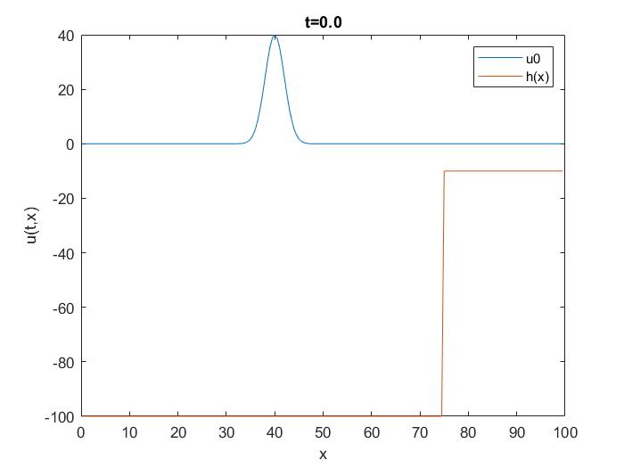
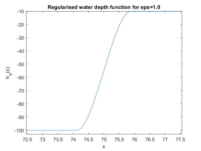
Figure 1. In the left plot, the graphics of the initial water level function $u_{0}(x)$ given by (3.6) and of the water depth $-h_{0}(x)$ are drawn (coloured by blue and orange, respectively). Here, the shore is a place between $75<x\leq 100$. In the right plot, for $\varepsilon=1.0$ the graphic of regularisation $h_{0,\varepsilon}(x)$ of the function $h_{0}(x)$ corresponding to Case 1 is given.

In this Section we carry out numerical experiments of the tsunami wave propagation in one- and two- dimensional cases. In particular, we analyse behaviours of the waves in singular topographies. Moreover, for 2D tsunami equation we develop a parallel computing algorithm to reduce the computational time. In particular, from the obtained simulations, we observe the appearance of a substantial reflected wave, travelling in the opposite direction from the point/line of singularity.

3.1. 1D case

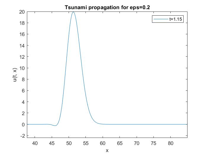
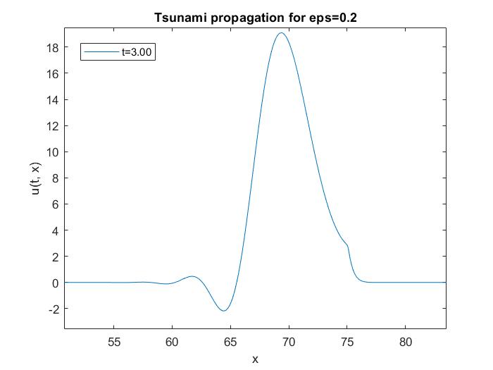
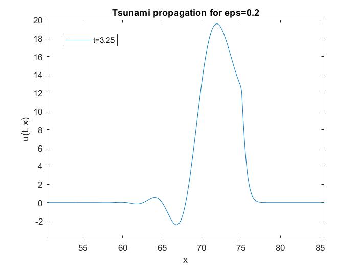
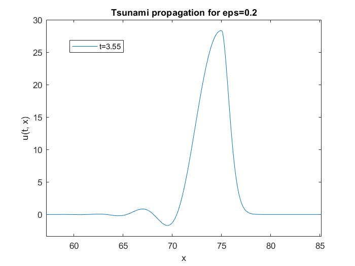
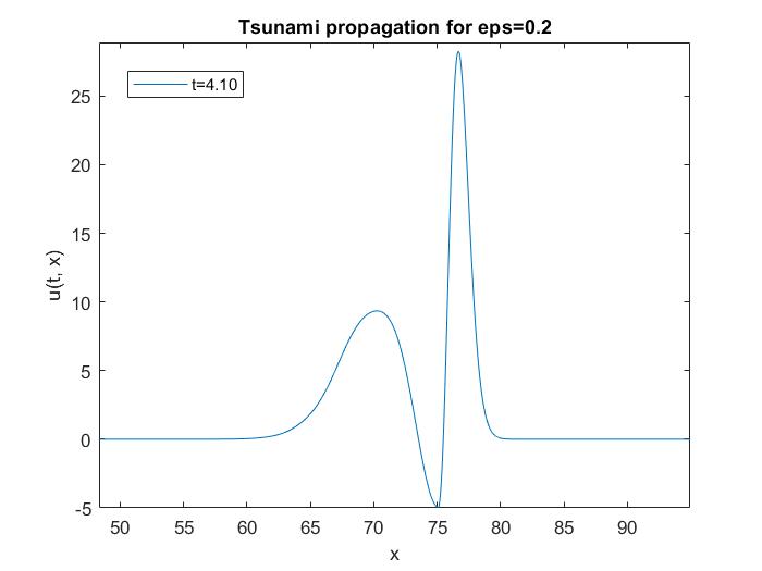
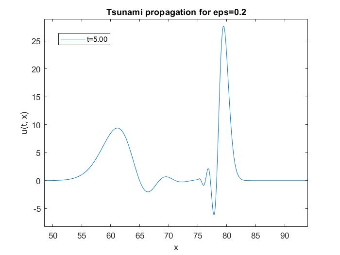
Figure 2. In these plots, an evolution of the solution of the regularised tsunami equation (3.5) is given in Case 1 for $\varepsilon=0.2$ at $t=1.15,3.00,3.25,3.55,4.10,5.00$.

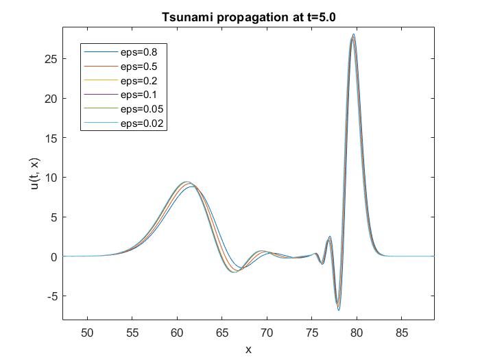
Figure 3. In this plot, the solution of the regularised tsunami equation (3.5) is given in Case 1 at time $t=5.00$ for different values of the parameter $\varepsilon$, namely, for $\varepsilon=0.02,0.05,0.1,0.2,0.5,0.8$.

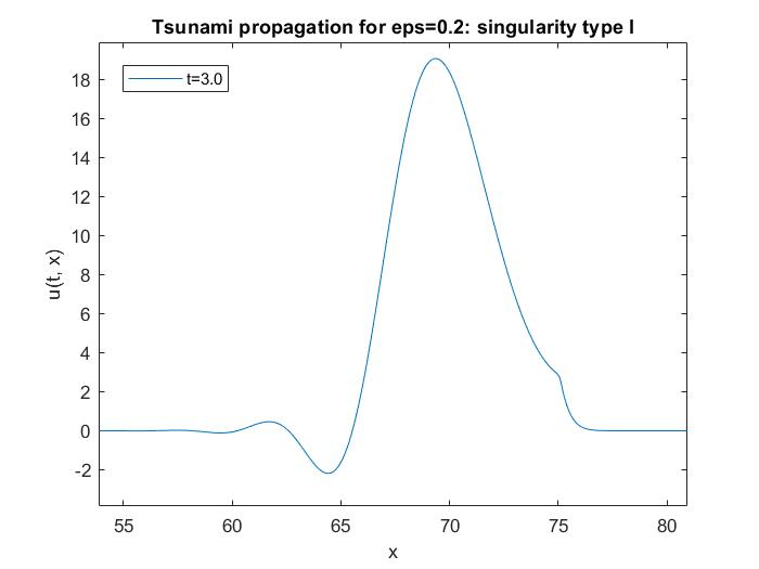
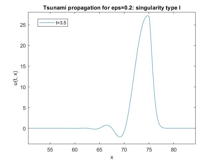
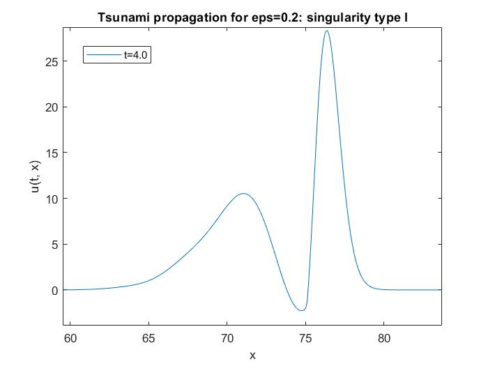
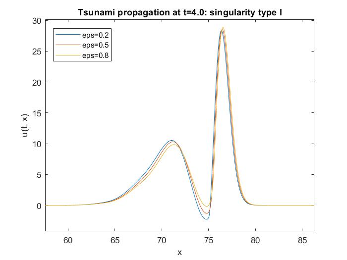
Figure 4. In these plots, the wave propagation corresponding to Case 2 is drawn at $t=3.0,3.5,4.0$. The right bottom plot shows that the solution of the regularised problem (3.5) with the water depth function $h(x):=h_{1}(x)$ is stable under the changing parameter $\varepsilon$.

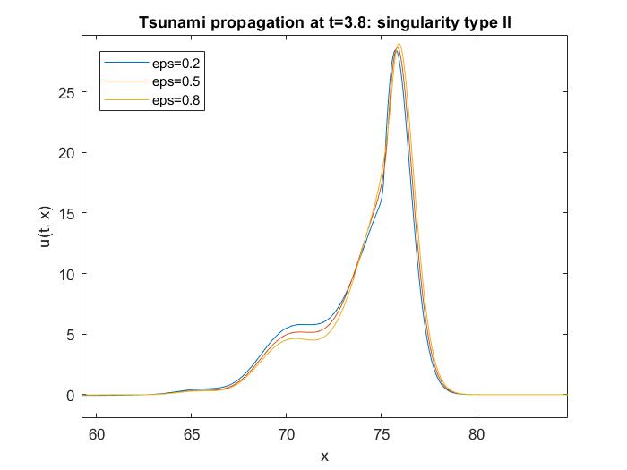
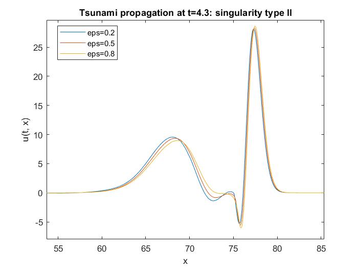
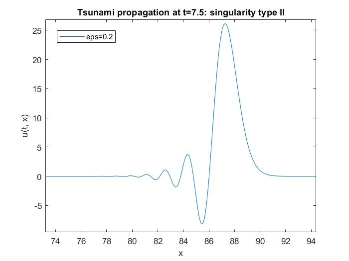
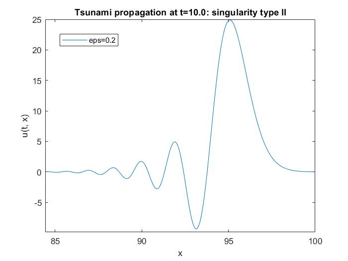
Figure 5. In these plots, the wave propagation corresponding to Case 3 is drawn at $t=3.8,4.3$ for $\varepsilon=0.2,0.5,0.8$ and at $t=7.5,10.0$ for $\varepsilon=0.2$. The plots show that the solution of the regularised problem (3.5) with the water depth function $h(x):=h_{2}(x)$ is stable under the changing parameter $\varepsilon$.

Here, we consider 1D tsunami wave propagation equation

(3.1) $$u_{tt}(t,x)-\partial_{x}\left(h(x)\partial_{x}u(t,x)\right)=0,\,\,\,(t,x)\in(0,T)\times\left(0,100\right),$$

with the initial conditions

$$u(0,x)=u_{0}(x),\,u_{t}(0,x)=u_{1}(x),$$

for all $x\in\left[0,100\right].$

In this work we are interested in the singular cases of the coefficient $h(x)$. Even, we can allow them to be distributional, in particular, to have $\delta$-like or $\delta^{2}$-like singularities. As it was theoretically outlined in [RT17a] and [RT17b], we start to analyse our problem by regularising a distributional valued function $h(x)$ by a parameter $\varepsilon$, that is, we set

(3.2) $$h_{\varepsilon}(x):=(h*\varphi_{\varepsilon})(x)$$

as the convolution with the mollifier

(3.3) $$\varphi_{\varepsilon}(x)=\frac{1}{\varepsilon}\varphi(x/\varepsilon),$$

where $\varphi(x)=c\exp{\left(\frac{1}{x^{2}-1}\right)}$ for $|x|<1,$ and $\varphi(x)=0$ otherwise. Here $c\simeq 2.2523$ to get $\int\limits_{-\infty}^{\infty}\varphi(x)dx=1.$

First, we study the following model situation:

• Case 1, when the water depth function $h(x)$ is given by

  (3.4) $$h_{0}(x)=\left\{\begin{array}[]{l}100,\,\,\,0\leq x<75,\\ 10,\,\,\,75\leq x\leq 100.\end{array}\right.$$

As the second step, we study singular situations:

• Case 2, when the water depth function $h(x)$ has a singularity. That is,

  $$h_{1}(x):=h_{0}(x)+\delta(x-70),$$

  where $\delta$ is Dirac’s function. By regularisation process described in above, we get

  $$h_{1,\varepsilon}(x)=h_{0,\varepsilon}(x)+\varphi_{\varepsilon}(x-70).$$

• Case 3, when the water depth function $h(x)$ has even more higher order of singularity, namely,

  $$h_{2}(x)=h_{0}(x)+\delta^{2}(x-70),$$

  in the sense that

  $$h_{2,\varepsilon}(x):=h_{0,\varepsilon}(x)+\varphi_{\varepsilon}^{2}(x-70).$$

In what follows, we investigate all three cases.

As it was adjusted in the theoretical part, instead of (3.1) we study the following regularised problem

(3.5) $$\partial^{2}_{tt}u_{\varepsilon}(t,x)-\partial_{x}\left(h_{\varepsilon}(x)\partial_{x}u_{\varepsilon}(t,x)\right)=0,\,\,\,(t,x)\in\left(0,T\right)\times\left(0,100\right),$$

with the Cauchy data

$$u_{\varepsilon}(0,x)=u_{0}(x),\,\partial_{t}u_{\varepsilon}(0,x)=u_{1}(x),$$

for all $x\in\left[0,100\right].$

For our tests, we take $u_{1}(x)\equiv 0$ and

(3.6) $$u_{0}(x)=40\exp({-(x-40)^{2}/8}).$$

Now, let us analyse the results of the numerical simulations. Figure 1 shows the graphics of the initial water level function $u_{0}(x)$ and the depth function $h(x):=h_{0}(x)$. In particular, for $\varepsilon=1.0$ the graphic of regularisation $h_{0,\varepsilon}(x)$ of the function $h_{0}(x)$ corresponding to Case 1 is also given. The function $h_{0}(x)$ has discontinuity at point $75$.

In Figure 2 for Case 1 we study an evolution of the solution of the regularised tsunami equation (3.5) for $\varepsilon=0.2$ at $t=1.15,3.00,3.25,3.55,4.10,5.00$. From the pictures we observe that the height of the wave is starting to increase as reaching the discontinuity point. Also, a reflected wave appears.

In Figure 3 we compare the solution of the regularised tsunami equation (3.5) for $\varepsilon=0.02,0.05,$ $0.1,0.2,0.5,0.8$ at time $t=5.00$ in Case 1. From the plot we can see that the solution $u_{\varepsilon}(t,x)$ of the regularised problem (3.5) is stable as $\varepsilon\to 0$.

Figures 4 and 5 illustrate the wave propagation corresponding to singular Cases 2 and 3 at different times. The plots show that the solutions of the regularised problem (3.5) with the water depth functions $h(x):=h_{1}(x)$ and $h(x):=h_{2}(x)$ are stable under the changing parameter $\varepsilon$.

In 1D case, for numerical computations we use the Crank-Nicolson method. All simulations are made in Math Lab 2018b. For all simulations we take $\Delta t=0.05,\Delta x=0.005.$

3.2. Limiting behaviour as $\varepsilon\to 0$

As we see from the graphs, it appears that the regularised solutions may have a limit as $\varepsilon\to 0$.

3.2.1. Discontinuous case

For illustration of this limiting behaviour as $\varepsilon\to 0$ of the solution of the regularised problems, as an example, we investigate Case 1 in more details. First of all, let us fix moments of $\varepsilon$ at $\varepsilon_{1}$ and $\varepsilon_{2}$. So, we will study the difference of the solution of the equation (3.5) with the initial data as in (3.6) at these two moments of $\varepsilon$, namely, $\|u_{\varepsilon_{1}}(t,\cdot)-u_{\varepsilon_{2}}(t,\cdot)\|_{L^{2}}$, and its limit as $\varepsilon_{1},\varepsilon_{2}\to 0$. Indeed, we have

(3.7) $$U_{tt}(t,x)-\partial_{x}\left(h_{\varepsilon_{1}}(x)\partial_{x}U(t,x)\right)=\partial_{x}\left(H(x)\partial_{x}u_{\varepsilon_{2}}(t,x)\right),$$

with the Cauchy data

$$U(0,x)=0,\,U_{t}(0,x)=0,$$

where $U:=[u_{\varepsilon_{1}}-u_{\varepsilon_{2}}]$ and $H:=[h_{\varepsilon_{1}}-h_{\varepsilon_{2}}]$.

Since the solution $U$ linearly depends on $H$, we start by calculating it:

$$\begin{split}H(x)&=h_{\varepsilon_{1}}(x)-h_{\varepsilon_{2}}(x)=(h*\varphi_{\varepsilon_{1}})(x)-(h*\varphi_{\varepsilon_{2}})(x)\\ &=\int\limits_{-\infty}^{\infty}h(s)\frac{1}{\varepsilon_{1}}\varphi\left(\frac{x-s}{\varepsilon_{1}}\right)ds-\int\limits_{-\infty}^{\infty}h(s)\frac{1}{\varepsilon_{2}}\varphi\left(\frac{x-s}{\varepsilon_{2}}\right)ds.\end{split}$$

Taking into account that we are considering Case 1 and using an explicit form of $h(x)$, we get

$$\begin{split}H(x)=&100\left[\int\limits_{x-\varepsilon_{1}}^{75}\frac{1}{\varepsilon_{1}}\varphi\left(\frac{x-s}{\varepsilon_{1}}\right)ds-\int\limits_{x-\varepsilon_{2}}^{75}\frac{1}{\varepsilon_{2}}\varphi\left(\frac{x-s}{\varepsilon_{2}}\right)ds\right]\\ &+10\left[\int\limits_{75}^{x+\varepsilon_{1}}\frac{1}{\varepsilon_{1}}\varphi\left(\frac{x-s}{\varepsilon_{1}}\right)ds-\int\limits_{75}^{x+\varepsilon_{2}}\frac{1}{\varepsilon_{2}}\varphi\left(\frac{x-s}{\varepsilon_{2}}\right)ds\right]\\ =&100\int\limits^{\frac{x-75}{\varepsilon_{2}}}_{\frac{x-75}{\varepsilon_{1}}}\varphi(z)dz-10\int\limits^{\frac{x-75}{\varepsilon_{2}}}_{\frac{x-75}{\varepsilon_{1}}}\varphi(z)dz=90\int\limits^{\frac{x-75}{\varepsilon_{2}}}_{\frac{x-75}{\varepsilon_{1}}}\varphi(z)dz.\end{split}$$

Since $\varphi(x)$ is a compactly supported function, from the above calculations it is easy to see that for the sufficiently small parameters $\varepsilon_{1}$ and $\varepsilon_{2}$ the function $H(x)$ is identically zero.

Remark 3.1.

Note that if instead of $\varphi_{\varepsilon_{2}}$ we take another mollifier $\psi_{\varepsilon_{2}}$ with the same properties then we obtain

$$\begin{split}H(x)=&100\left[\int\limits_{x-\varepsilon_{1}}^{75}\frac{1}{\varepsilon_{1}}\varphi\left(\frac{x-s}{\varepsilon_{1}}\right)ds-\int\limits_{x-\varepsilon_{2}}^{75}\frac{1}{\varepsilon_{2}}\psi\left(\frac{x-s}{\varepsilon_{2}}\right)ds\right]\\ &+10\left[\int\limits_{75}^{x+\varepsilon_{1}}\frac{1}{\varepsilon_{1}}\varphi\left(\frac{x-s}{\varepsilon_{1}}\right)ds-\int\limits_{75}^{x+\varepsilon_{2}}\frac{1}{\varepsilon_{2}}\psi\left(\frac{x-s}{\varepsilon_{2}}\right)ds\right]\\ =&100\int\limits^{1}_{\frac{x-75}{\varepsilon_{1}}}\varphi(z)dz-100\int\limits^{1}_{\frac{x-75}{\varepsilon_{2}}}\psi(z)dz+10\int\limits^{\frac{x-75}{\varepsilon_{2}}}_{-1}\varphi(z)dz-10\int\limits^{\frac{x-75}{\varepsilon_{1}}}_{-1}\psi(z)dz\\ =&100\int\limits^{\frac{x-75}{\varepsilon_{2}}}_{\frac{x-75}{\varepsilon_{1}}}\varphi(z)dz+100\int\limits^{1}_{\frac{x-75}{\varepsilon_{2}}}(\varphi-\psi)(z)dz+10\int\limits^{\frac{x-75}{\varepsilon_{2}}}_{-1}(\varphi-\psi)(z)dz+10\int\limits^{\frac{x-75}{\varepsilon_{2}}}_{\frac{x-75}{\varepsilon_{1}}}\psi(z)dz\\ =&100\int\limits^{\frac{x-75}{\varepsilon_{2}}}_{\frac{x-75}{\varepsilon_{1}}}\varphi(z)dz+90\int\limits^{1}_{\frac{x-75}{\varepsilon_{2}}}(\varphi-\psi)(z)dz+10\int\limits^{\frac{x-75}{\varepsilon_{2}}}_{\frac{x-75}{\varepsilon_{1}}}\psi(z)dz.\end{split}$$

Interesting to note that the last expression is also tending to zero as $\varepsilon_{1},\varepsilon_{2}\to 0$.

Thus, we conclude for the sufficiently small parameters $\varepsilon_{1}$ and $\varepsilon_{2}$ the solution $U(t,x)$ of the problem (3.7) is identically zero. Finally, it shows that

$$\|u_{\varepsilon_{1}}(t,\cdot)-u_{\varepsilon_{2}}(t,\cdot)\|_{L^{2}}=0,$$

as $\varepsilon_{1},\varepsilon_{2}\to 0$.

Therefore, a surprising conclusion is that while, in general, the solution of the equation (3.1) may not exist in a ‘classical’ sense for singular $h$, the limit (as $\varepsilon\to 0$) of the very weak solution family $u_{\varepsilon}$ may exist. We can then talk about the limiting very weak solution of (3.1) as the limit of the family $u_{\varepsilon}$.

3.2.2. Irregular case

For illustration of this limiting behaviour as $\varepsilon\to 0$ of the solution of the regularised problems, as a second example, we investigate Case 2 in more details. First of all, let us fix moments of $\varepsilon$ at $\varepsilon_{1}$ and $\varepsilon_{2}$. So, we will study the difference of the solution of the equation (3.5) with the initial data as in (3.6) at these two moments of $\varepsilon$, namely, $\|u_{\varepsilon_{1}}(t,\cdot)-u_{\varepsilon_{2}}(t,\cdot)\|_{L^{2}}$, and its limit as $\varepsilon_{1},\varepsilon_{2}\to 0$. Indeed, we have

(3.8) $$U_{tt}(t,x)-\partial_{x}\left(h_{\varepsilon_{1}}(x)\partial_{x}U(t,x)\right)=\partial_{x}\left(H(x)\partial_{x}u_{\varepsilon_{2}}(t,x)\right),$$

with the Cauchy data

$$U(0,x)=0,\,U_{t}(0,x)=0,$$

where $U:=[u_{\varepsilon_{1}}-u_{\varepsilon_{2}}]$ and $H:=[h_{\varepsilon_{1}}-h_{\varepsilon_{2}}]$.

By changing

$$V(t,x):=\int\limits_{-\infty}^{x}U(t,s)ds,$$

instead of the equation (3.8) we get

(3.9) $$V_{tt}(t,x)-h_{\varepsilon_{1}}(x)\partial_{xx}V(t,x)=H(x)\partial_{x}u_{\varepsilon_{2}}(t,x),$$

with the Cauchy data

$$V(0,x)=0,\,V_{t}(0,x)=0.$$

Repeating the above procedure, let us calculate $H$:

$$\begin{split}H(x)&=h_{\varepsilon_{1}}(x)-h_{\varepsilon_{2}}(x)=(h*\varphi_{\varepsilon_{1}})(x)-(h*\varphi_{\varepsilon_{2}})(x)\\ &=\int\limits_{-\infty}^{\infty}h(s)\frac{1}{\varepsilon_{1}}\varphi\left(\frac{x-s}{\varepsilon_{1}}\right)ds-\int\limits_{-\infty}^{\infty}h(s)\frac{1}{\varepsilon_{2}}\varphi\left(\frac{x-s}{\varepsilon_{2}}\right)ds.\end{split}$$

Taking into account that we are considering Case 2 and using an explicit form of $h(x)$, we get

$$H(x)=A(x)+D(x),$$

where

$$A(x)=90\int\limits^{\frac{x-75}{\varepsilon_{2}}}_{\frac{x-75}{\varepsilon_{1}}}\varphi(z)dz\,\,\,\,\hbox{and}\,\,\,\,D(x)=\frac{1}{\varepsilon_{1}}\varphi\left(\frac{x-70}{\varepsilon_{1}}\right)-\frac{1}{\varepsilon_{2}}\varphi\left(\frac{x-70}{\varepsilon_{2}}\right).$$

Since $\varphi(x)$ is a compactly supported function, from the above calculations it is easy to see that for the sufficiently small parameters $\varepsilon_{1}$ and $\varepsilon_{2}$ the function $A(x)$ is identically zero. Also, we note that the function $D(x)$ has a compact support

$$\operatorname{supp}D\subset[70-\max(\varepsilon_{1},\varepsilon_{2}),70+\max(\varepsilon_{1},\varepsilon_{2})].$$

Without loss of generality, we assume that $\varepsilon_{1}\geq\varepsilon_{2}$. Then it is clear that

$$\operatorname{supp}D=\operatorname{supp}_{sing}h_{\varepsilon_{1}}\subset[70-\varepsilon_{1},70+\varepsilon_{1}]=:\Omega_{\varepsilon_{1}}.$$

Note that when $x\in\mathbb{R}\setminus\Omega_{\varepsilon_{1}}$ we have the Discontinuous case. Now we are interested in the case when $x\in\Omega_{\varepsilon_{1}}$. Thus, for small enough $\varepsilon_{1}$, we have

$$\varepsilon_{1}V_{tt}(t,x)-\left[\varepsilon_{1}h_{0,\varepsilon_{1}}(x)+\varphi\left(\frac{x-70}{\varepsilon_{1}}\right)\right]\partial_{xx}V(t,x)=\varepsilon_{1}H(x)\partial_{x}u_{\varepsilon_{2}}(t,x),$$

and by neglecting the small terms, we arrive at the elliptic type problem

(3.10) $$-\varphi\left(\frac{x-70}{\varepsilon_{1}}\right)\partial_{xx}V(t,x)=\left(\varphi\left(\frac{x-70}{\varepsilon_{1}}\right)-\frac{\varepsilon_{1}}{\varepsilon_{2}}\varphi\left(\frac{x-70}{\varepsilon_{2}}\right)\right)\partial_{x}u_{\varepsilon_{2}}(t,x).$$

Dividing both sides of (3.10) by $\varphi\left(\frac{x-70}{\varepsilon_{1}}\right)$, we obtain

(3.11) $$-\partial_{xx}V(t,x)=\left(1-\frac{\varepsilon_{1}}{\varepsilon_{2}}\hat{\varphi}(x,\varepsilon_{2})\right)\partial_{x}u_{\varepsilon_{2}}(t,x),$$

where $\operatorname{supp}{\hat{\varphi}}=\Omega_{\varepsilon_{2}}$ and $x\in\Omega_{\varepsilon_{1}}$. By integrating over $\int_{-\infty}^{x}$ and taking into account that $U(t,x)=\partial_{x}V(t,x)$, we arrive at

(3.12) $$U(t,x)=u_{\varepsilon_{2}}(t,70+\varepsilon_{1})-u_{\varepsilon_{2}}(t,70-\varepsilon_{1})+\frac{\varepsilon_{1}}{\varepsilon_{2}}\int\limits_{70-\varepsilon_{2}}^{\min(70+\varepsilon_{2},x)}\hat{\varphi}(s,\varepsilon_{2})\partial_{s}u_{\varepsilon_{2}}(t,s)ds,$$

for $x\in\Omega_{\varepsilon_{1}}$.

Now we need to estimate (3.12) in $L^{2}$-norm. For this, by adapting the energy conservation formula (2.7) to $u_{\varepsilon_{2}}$, we obtain

(3.13) $$\begin{split}\|\partial_{x}u_{\varepsilon_{2}}(t,\cdot)\|_{L^{2}}^{2}\leq\frac{1}{10}\|h_{\varepsilon_{2}}^{\frac{1}{2}}\partial_{x}u_{0}\|_{L^{2}}^{2}&=\frac{1}{10}\int\limits_{\mathbb{R}}h_{\varepsilon_{2}}(s)|\partial_{x}u_{0}(s)|^{2}ds\\ &=\frac{1}{10}\int\limits_{\mathbb{R}}\partial_{s}\hat{h}_{\varepsilon_{2}}(s)|\partial_{s}u_{0}(s)|^{2}ds,\end{split}$$

where $h_{\varepsilon_{2}}(s):=\partial_{s}\hat{h}_{\varepsilon_{2}}(s)$. Integrating by parts and taking into account the properties of $u_{0}$, from (3.13) we get

(3.14) $$\begin{split}\|\partial_{x}u_{\varepsilon_{2}}(t,\cdot)\|_{L^{2}}^{2}&\leq\frac{1}{10}\int\limits_{\mathbb{R}}\partial_{s}\hat{h}_{\varepsilon_{2}}(s)|\partial_{s}u_{0}(s)|^{2}ds\\ &=\frac{1}{5}\int\limits_{\mathbb{R}}\hat{h}_{\varepsilon_{2}}(s)|\partial_{s}^{2}u_{0}(s)\partial_{s}u_{0}(s)|ds\\ &=\frac{1}{5}\|\hat{h}_{\varepsilon_{2}}\|_{L^{\infty}}\|\partial_{s}^{2}u_{0}\|_{L^{2}}\|\partial_{s}u_{0}\|_{L^{2}}.\end{split}$$

The term $\|\partial_{x}u_{\varepsilon_{2}}(t,\cdot)\|_{L^{2}}$ does not blow up as $\varepsilon_{2}\to 0$ since $\hat{h}_{\varepsilon_{2}}\to\hat{h}\in L^{\infty}$ as $\varepsilon_{2}\to 0$. Repeating the process for $u_{\varepsilon_{2}}$, one obtains that $u_{\varepsilon_{2}}$ is also regular in $\Omega_{\varepsilon_{1}}$.

Since for $x\in\mathbb{R}\setminus\Omega_{\varepsilon_{1}}$ the function $U(t,x)$ equal the solution corresponding to Case 1, and due to the fact that the volume of the domain $\Omega_{\varepsilon_{1}}$ tends to zero as $\varepsilon_{1}\to 0$, we conclude that for the sufficiently small parameters $\varepsilon_{1}$ and $\varepsilon_{2}$ the solution $U(t,x)$ of the problem (3.8) tends to zero. Finally, it shows that

$$\|u_{\varepsilon_{1}}(t,\cdot)-u_{\varepsilon_{2}}(t,\cdot)\|_{L^{2}}\to 0,$$

as $\varepsilon_{1},\varepsilon_{2}\to 0$.

Therefore, a surprising conclusion is that while, in general, the solution of the equation (3.1) may not exist in a ‘classical’ sense for singular $h$, the limit (as $\varepsilon\to 0$) of the very weak solution family $u_{\varepsilon}$ may exist. We can then talk about the limiting very weak solution of (3.1) as the limit of the family $u_{\varepsilon}$.

3.2.3. Tests for singularities

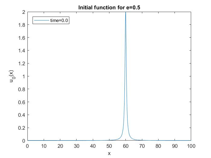
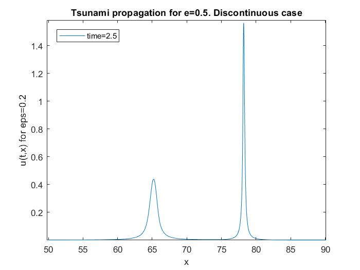
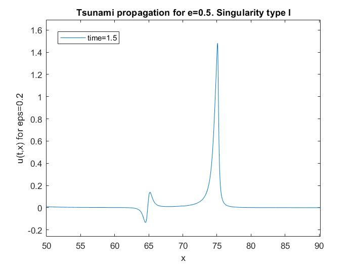
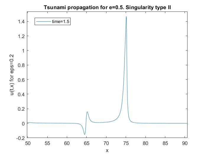
Figure 6. In these plots, the initial function $u_{0}$ given by (3.16) and the wave propagation corresponding to the discontinuous and singular type I and II cases are drawn for $e=0.5$, respectively. All simulations are done for $\varepsilon=0.2$.

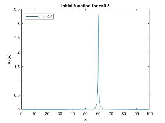
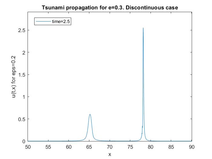
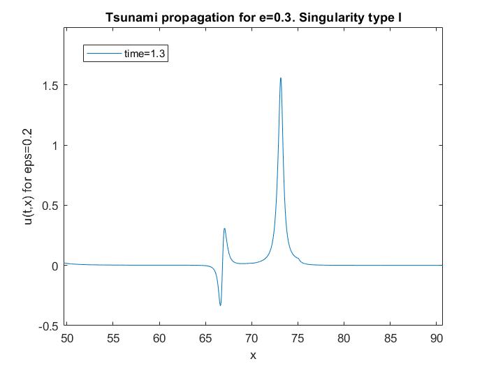
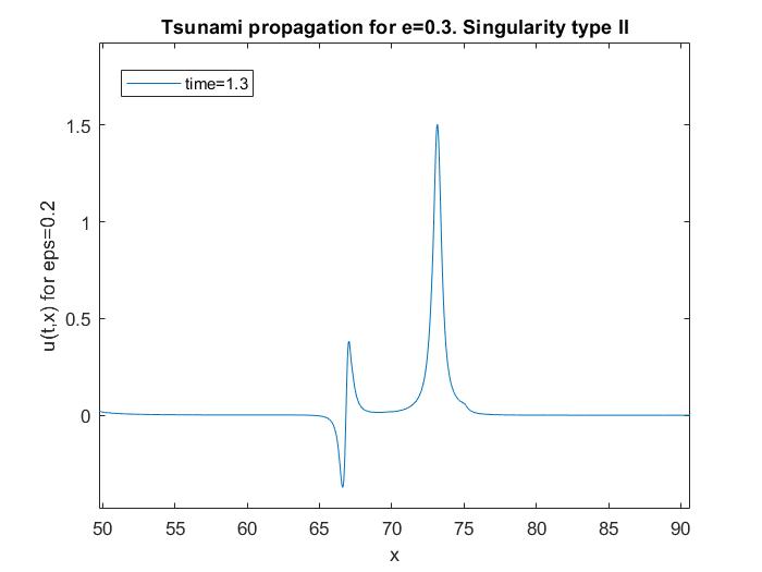
Figure 7. In these plots, the initial function $u_{0}$ given by (3.16) and the wave propagation corresponding to the discontinuous and singular type I and II cases are drawn for $e=0.3$, respectively. All simulations are done for $\varepsilon=0.2$.

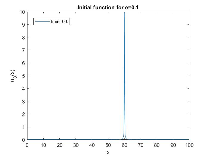
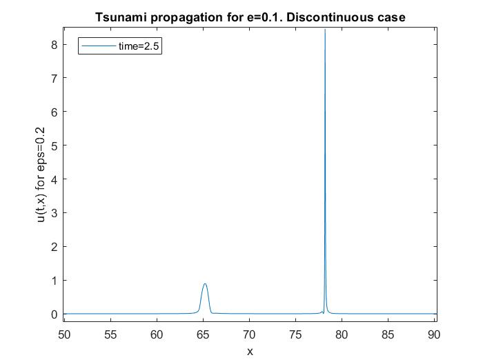
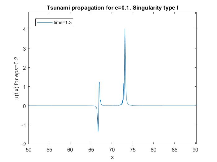
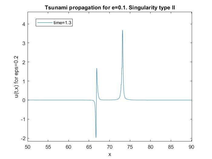
Figure 8. In these plots, the initial function $u_{0}$ given by (3.16) and the wave propagation corresponding to the discontinuous and singular type I and II cases are drawn for $e=0.1$, respectively. All simulations are done for $\varepsilon=0.2$.

To investigate singularities, we consider

• Discontinuous case, when the water depth function $h(x)$ is given by

  (3.15) $$h_{0}(x)=\left\{\begin{array}[]{l}100,\,\,\,0\leq x<75,\\ 10,\,\,\,75\leq x\leq 100.\end{array}\right.$$

• Singular type I case, when the water depth function $h(x)$ has a singularity. That is,

  $$h_{1}(x):=h_{0}(x)+100\delta(x-70),$$

  where $\delta$ is Dirac’s function. By regularisation process described in above, we get

  $$h_{1,\varepsilon}(x)=h_{0,\varepsilon}(x)+100\varphi_{\varepsilon}(x-70).$$

• Singular type II case, when the water depth function $h(x)$ has even more higher order of singularity, namely,

  $$h_{2}(x)=h_{0}(x)+100\delta^{2}(x-70),$$

  in the sense that

  $$h_{2,\varepsilon}(x):=h_{0,\varepsilon}(x)+100\varphi_{\varepsilon}^{2}(x-70).$$

Here, we simulate the cases of $h$ considering instead of $u_{0}$ given by (3.6) the function

(3.16) $$u_{0}(x)=\frac{e}{(x-60)^{2}+e^{2}},$$

for $e\in\mathbb{R}_{+}$.

In Figures 6-8 we test for $e=0.5,0.3,0.1.$ The reason for this investigation is to see the strength of the singularity in the reflected wave. We observe that the singularity of the reflected wave (the sharpness of the peak) is less than that of the main wave in the Case I, while the reflected singularity seems to be of the same strength in Cases II and III. In this respect, the behaviour in Case I resembles more that of the conical refraction corresponding to multiplicities (as in [KR07]), while Cases II and III appear to be more like acoustic echo-type effects for singular media (as in [MRT19]).

In all cases the second wave is smaller in size. The reflected wave has only one positive component in Case I, while it has both positive and negative parts in Cases II and III.

3.3. 2D case

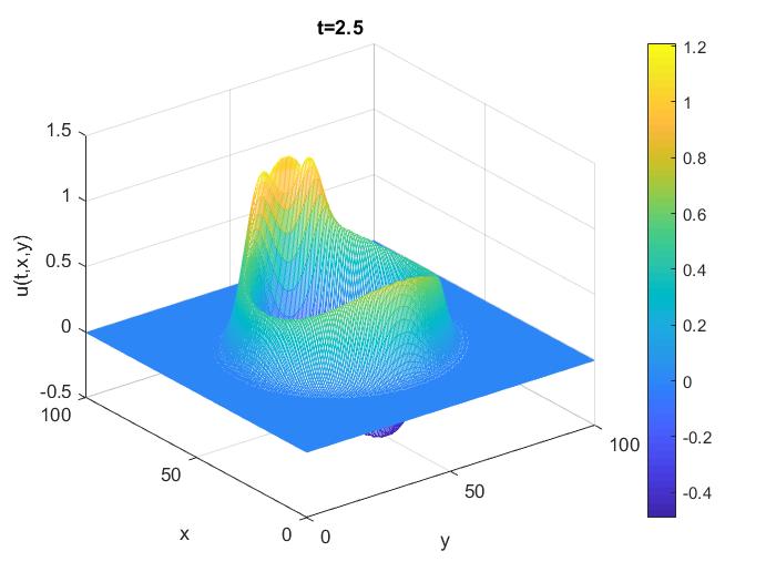
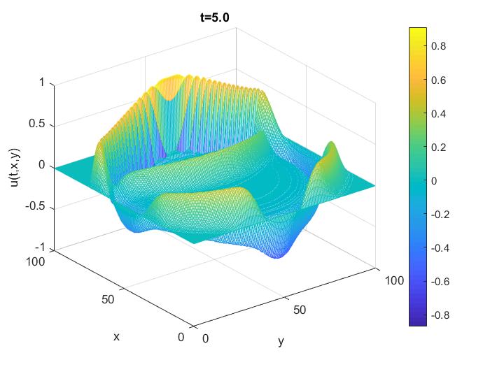
Figure 9. Displacement of the wave corresponding to the equation (3.18) for $\varepsilon=0.8$ at $t=2.5$ and $t=5.0$.

In the domain $\left[0,T\right]\times\left[0,100\right]\times\left[0,100\right]$, we simulate the following boundary value problem for the 2D tsunami equation

$$u_{tt}(t,x,y)-[\partial_{x}\left(H(x,y)\partial_{x}u(t,x,y)\right)+\partial_{y}\left(H(x,y)\partial_{y}u(t,x,y)\right)]=0,$$

with the initial data

$$u(0,x,y)=u_{0}(x,y),\,\,\,u_{t}(0,x,y)=u_{1}(x,y),\,\,\,x,y\in\left[0,100\right],$$

and boundary conditions

$$u(t,0,y)=0,\,u(t,100,y)=0,\,u(t,x,0)=0,\,u(t,x,100)=0,$$

for $x,y\in\left[0,100\right],$ for $t\in\left[0,T\right]$.

Now we introduce a space-time grid with steps $h_{x},h_{y},\tau$ in the variables $t,x,y$, respectively:

(3.17) $$\omega_{h_{x},h_{y}}^{\tau}={\{t_{k}=k\tau,\,\,k=\overline{0,M};x_{i}=ih_{x},y_{j}=jh_{y},\,\,i,j=\overline{0,N}}\},$$

where $\tau M=T,h_{x}N=h_{y}N=100$. For numerically solving this problem we use an implicit finite difference scheme [Sam77] and the cyclic reduction method [GS11].

In the two-dimensional model, we consider ’Case 1’ corresponding to 1D simulations. For the water depth function $H(x,y)$ we put

$$H(x,y):=h_{0}(x),$$

in $x$ variable and constant in $y$ variable. Here $h_{0}(x)$ is as in (3.15). Eventually, for the regularisation of $H(x,y)$ we get $H_{\varepsilon}(x,y)=h_{0,\varepsilon}(x).$ For the simulations we solve the following regularised equation

(3.18) $$u_{tt}(t,x,y)-[\partial_{x}\left(H_{\varepsilon}(x,y)\partial_{x}u(t,x,y)\right)+\partial_{y}\left(H_{\varepsilon}(x,y)\partial_{y}u(t,x,y)\right)]=0,$$

with the initial functions

$$u_{0}(x,y)=50\exp({-((x-40)^{2}+(y-50)^{2})/8})$$

and $u_{1}(x,y)=0$.

In 2D case, numerical computations and simulations are made in python by using the cyclic reduction method. For all simulations we take $\Delta t=0.5,\Delta x=0.05,\Delta y=0.05.$

4. GPU computing

Modeling a wider area and long-term modeling using a standard personal computer requires more time, and it is often very important to reduce the computation time. Modern graphical processing units provide a powerful instrument for parallel processing with massively data-parallel throughput-oriented multi-core processors capable of providing TFLOPS of computing performance and quite high memory bandwidth. So with the aim of reducing computation time in this work, we use GPU computing.

In this section we show the results obtained on a desktop computer with configuration 4352 cores GeForce RTX 2080 TI, NVIDIA GPU together with a CPU Intel Core(TM) i7-9800X, 3.80 GHz, RAM 64Gb. Simulation parameters are configured as follows. Mesh size is uniform in both directions with $\Delta x=\Delta y$ and numerical time step $\Delta t$ is 0.05, and simulation time is $T=5.0$, therefore the total number of time steps is 100. To present more realistic data, we tested five cases with computational domain sizes of $256\times 256,512\times 512,1024\times 1024,2048\times 2048$ and $4096\times 4096$.

The performance of a parallel algorithm is determined by calculating its speedup. The speedup is defined as the ratio of the execution time of the sequential algorithm for a particular problem to the execution time of the parallel algorithm.

$$\mathrm{Speedup}=\frac{\mathrm{CPUtime}}{\mathrm{GPUtime}}$$

In Table 1 we report the execution times in seconds for serial (CPU time) and CUDA (GPU time) implementation of cyclic reduction method to the problem (3.18) together with the values of the speedup.

Table 1. Execution timing and speedup with the Intel Core(TM) i7-9800X, 3.80 GHz, NVIDIA RTX 2080 TI

Domain sizes	CPU time	GPU time	Speedup
$256\times 256$	0.91	0.88	1.03
$512\times 512$	3.73	2.07	1.8
$1024\times 1024$	15.92	7.16	2.22
$2048\times 2048$	64.8	20.30	3.19
$4096\times 4096$	280.54	62.76	4.47

References

- [ADD19] A. A. Abdalazeez, I. Didenkulova, D. Dutykh. Nonlinear deformation and run-up of single tsunami waves of positive polarity: numerical simulations and analytical predictions. Nat. Hazards Earth Syst. Sci., 19, 2905–2913, 2019.
- [ART19] A. Altybay, M. Ruzhansky, N. Tokmagambetov. Wave equation with distributional propagation speed and mass term: Numerical simulations. Appl. Math. E-Notes, 19 (2019), 552–562.
- [ARST20a] A. Altybay, M. Ruzhansky, M. E. Sebih, N. Tokmagambetov. Fractional Klein-Gordon equation with strongly singular mass term. Preprint, arXiv:2004.10145 (2020).
- [ARST20b] A. Altybay, M. Ruzhansky, M. E. Sebih, N. Tokmagambetov. Fractional Schrödinger Equations with potentials of higher-order singularities. Preprint, arXiv:2004.10182 (2020).
- [ARST20c] A. Altybay, M. Ruzhansky, M. E. Sebih, N. Tokmagambetov. The heat equation with singular potentials. Preprint, arXiv:2004.11255 (2020).
- [Behr10] J. Behrens Numerical Methods in Support of Advanced Tsunami Early Warning. In: Freeden W., Nashed M.Z., Sonar T. (eds) Handbook of Geomathematics. Springer, (2010).
- [BD15] J. Behrens, F. Dias. New computational methods in tsunami science. Phil. Trans. R. Soc. A, 373: 20140382, 2015.
- [DD07] F. Dias, D. Dutykh. Dynamics of tsunami waves. Extreme Man-Made and Natural Hazards in Dynamics of Structures, (2007) 201–224.
- [DDORS14] F. Dias, D. Dutykh, L. O Brien, E. Renzi, T. Stefanakis. On the Modelling of Tsunami Generation and Tsunami Inundation. Procedia IUTAM, Vol. 10 (2014), 338–355.
- [ER18] M. R. Ebert, M. Reissig. Methods for Partial Differential Equations. Birkhäuser, 2018.
- [FJ98] F.G. Friedlander, M. Joshi. Introduction to the Theory of Distributions. Cambridge University Press, 1998.
- [GR15] C. Garetto, M. Ruzhansky. Hyperbolic second order equations with non-regular time dependent coefficients. Arch. Rational Mech. Anal., 217 (2015), no. 1, 113–154.
- [Gar20] C. Garetto. On the wave equation with multiplicities and space-dependent irregular coefficients. Preprint, arXiv:2004.09657 (2020).
- [GS11] D. Goddeke, R. Strzodka. Cyclic reduction tridiagonal solvers on GPUs applied to mixed-precision multigrid, Parallel and Distributed Systems, IEEE Transactions, 22:1, 22–32, 2011.
- [KR07] I. Kamotski, M. Ruzhansky. Regularity properties, representation of solutions and spectral asymptotics of systems with multiplicities, Comm. Partial Differential Equations, 32 (2007), 1–35.
- [Kun07] A. Kundu. Tsunami and Nonlinear Waves. Springer, 2007.
- [LGB11] R. J. LeVeque, D. L. George, M. J. Berger. Tsunami modelling with adaptively refined finite volume methods. Acta Numerica, pp. 211–289 (2011).
- [MRT19] J.C. Munoz, M. Ruzhansky and N. Tokmagambetov. Wave propagation with irregular dissipation and applications to acoustic problems and shallow water. Journal de Mathématiques Pures et Appliquées. Volume 123, March 2019, Pages 127–147.
- [Ren17] E. Renzi. Hydro-acoustic frequencies of the weakly compressible mild-slope equation. J. Fluid Mech., 812 (2017), 5–25.
- [RHH11] K. T. Ramadan H. S.Hassan, S. N. Hanna. Modeling of tsunami generation and propagation by a spreading curvilinear seismic faulting in linearized shallow-water wave theory. Applied Mathematical Modelling, 35 (2011) 61–79.
- [RS08] E. Renzi, P. Sammarco. Landslide tsunamis propagating along a plane beach. J. Fluid Mech., 598 (2008), 107–119.
- [RS10] E. Renzi, P. Sammarco. Landslide tsunamis propagating around a conical island. J. Fluid Mech., 650 (2010), 251–285.
- [RT17a] M. Ruzhansky, N. Tokmagambetov. Very weak solutions of wave equation for Landau Hamiltonian with irregular electromagnetic field. Lett. Math. Phys., 107 (2017) 591–618.
- [RT17b] M. Ruzhansky, N. Tokmagambetov. Wave equation for operators with discrete spectrum and irregular propagation speed. Arch. Rational Mech. Anal., 226 (3) (2017) 1161–1207.
- [Sam77] A. A. Samarskiy Teoriya raznostnykh skhem [theory of difference schemes]. Moscow. 1977. Pages 540–544.
- [Sch54] L. Schwartz. Sur l’impossibilite de la multiplication des distributions. C. R. Acad. Sci. Paris, 239 (1954) 847–848.
- [SW20] M.E. Sebih, J. Wirth. On a wave equation with singular dissipation. Preprint, Arxiv: 2002.00825 (2020).