Vertically Federated Graph Neural Network for Privacy-Preserving Node Classification

Abstract

Graph Neural Network (GNN) has achieved remarkable progresses in various real-world tasks on graph data. High-performance GNN models always depend on both rich features and complete edge information in graph. However, such information could possibly be isolated by different data holders in practice, which is the so-called data isolation problem. To solve this problem, in this paper, we propose Vertically Federated Graph Neural Network (VFGNN), a federated GNN learning paradigm for privacy-preserving node classification task under data vertically partitioned setting, which can be generalized to existing GNN models. Specifically, we split the computation graph into two parts. We leave the private data (i.e., features, edges, and labels) related computations on data holders, and delegate the rest of computations to a semi-honest server. We also propose to apply differential privacy to prevent potential information leakage from the server. We conduct experiments on three benchmarks and the results demonstrate the effectiveness of VFGNN.

1 Introduction

Graph Neural Network (GNN) has gained increasing attentions from both academy and industry due to its ability to model high-dimensional feature information and high-order adjacent information on both homogeneous and heterogeneous graphs Wu et al. (2019). An important ingredient for high-performance GNN models is high-quality graph data including rich node features and complete adjacent information. However, in practice, such information could possibly be isolated by different data holders, which is the so-called data isolation problem. Such a data isolation problem presents a serious challenge for the development of Artificial Intelligence, which becomes a hot research topic recently.

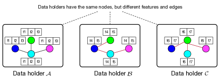
Figure 1: Problem description of vertically federated GNN.

Problem. Figure 1 shows a privacy-preserving node classification problem under vertically partitioned data setting. Here, we assume there are three data holders ($\mathcal{A}$, $\mathcal{B}$, and $\mathcal{C}$) and they have four same nodes. The node features are vertically split, i.e., $\mathcal{A}$ has $f1$, $f2$, and $f3$, $\mathcal{B}$ has $f4$ and $f5$, and $\mathcal{C}$ has $f6$ and $f7$. Meanwhile, $\mathcal{A}$, $\mathcal{B}$, and $\mathcal{C}$ may have their own edges. For example, $\mathcal{A}$ has social relation between nodes while $\mathcal{B}$ and $\mathcal{C}$ have payment relation between nodes. We also assume $\mathcal{A}$ is the party who has the node labels. The problem is to build federated GNN models using the graph data of $\mathcal{A}$, $\mathcal{B}$, and $\mathcal{C}$.

Related work. To date, many kinds of privacy-preserving machine learning models have been proposed, e.g., logistic regression Chen et al. (2021), decision tree Fang et al. (2021), and neural network Wagh et al. (2019). There are also several work on studying the privacy issues in GNN, e.g., graph publishing Sajadmanesh and Gatica-Perez (2020), GNN inference He et al. (2020), and federated GNN when data are horizontally partitioned Zheng et al. (2021); Wu et al. (2021). So far, few research has studied the problem of GNN when data are vertically partitioned, which popularly exists in practice. Unlike previous privacy-preserving machine learning models that assume only samples (nodes) are held by different parties and these samples have no relationship, our task is more challenging because GNN relies on the relationships between samples, which are also kept by different data holders.

Naive solution. A direct way to build privacy-preserving GNN is employing advanced cryptographic algorithms, such as homomorphic encryption (HE) and secure multi party computation (MPC) Mohassel and Zhang (2017). Such a pure cryptographic way can provide high security guarantees, however, it suffers high computation and communication costs, which limits their efficiency Osia et al. (2019).

Our solution. Instead, we propose VFGNN, a federated GNN learning paradigm for privacy-preserving node classification task under data vertically partitioned setting. Motivated by the existing work in split learning Vepakomma et al. (2018); Osia et al. (2019); Gu et al. (2018), we split the computation graph of GNN into two parts for privacy and efficiency concern, i.e., the private data related computations carried out by data holders and non-private data related computations conducted by a semi-honest server.

Specifically, data holders first apply MPC techniques to compute the initial layer of the GNN using private node feature information collaboratively, which acts as the feature extractor module, and then perform neighborhood aggregation using private edge information individually, similar as the existing GNNs Veličković et al. (2017), and finally get the local node embeddings. Next, we propose different combination strategies for a semi-honest server to combine local node embeddings from data holders and generate global node embeddings, based on which the server can conduct the successive non-private data related computations, e.g., the non-linear operations in deep network structures that are time-consuming for MPC techniques. Finally, the server returns the final hidden layer to the party who has labels to compute prediction and loss. Data holders and the server perform forward and back propagations to complete model training and prediction, during which the private data (i.e., features, edges, and labels) are always kept by data holders themselves. Here we assume data holders are honest-but-curious, and the server does not collude with data holders. We argue that this is a reasonable assumption since the server can be played by authorities such as governments or replaced by trusted execution environment Costan and Devadas (2016). Moreover, we adopt differential privacy, on the exchanged information between server and data holders (e.g., local node embeddings and gradient update), to further protect potential information leakage from the server.

Contributions. We summarize our main contributions as:

• We propose a novel VFGNN learning paradigm, which not only can be generalized to most existing GNNs, but also enjoys good accuracy and efficiency.

• We propose different combination strategies for the server to combine local node embeddings from data holders.

• We evaluate our proposals on three real-world datasets, and the results demonstrate the effectiveness of VFGNN.

2 Preliminaries

2.1 Security Model

In this paper, we assume the adversary is honest-but-curious (semi-honest). That is, data holders and the server strictly follow the protocol, but they also use all intermediate computation results to infer as much information as possible. We also assume that the server does not collude with any data holders. This security setting is similar as most existing work Mohassel and Zhang (2017); Hardy et al. (2017).

2.2 Additive Secret Sharing

Additive Secret Sharing has two main procedures. Shamir (1979). To additively share $\textbf{Shr}(\cdot)$ an $\ell$-bit value $a$ for party $i\in\mathcal{P}=\{1,...,I\}$, party $i$ generates {$a_{j}\in\mathds{Z}_{2^{\ell}},j\in\mathcal{P}$ and $j\neq i$} uniformly at random, sends $a_{j}$ to party $j$, and keeps $a_{i}=a-\sum_{j}a_{j}$ mod $2^{\ell}$. We use $\langle a\rangle_{i}=a_{i}$ to denote the share of party $i$. To reconstruct $\textbf{Rec}(\cdot,\cdot)$ a shared value $\langle a\rangle$, each party $i$ sends $\langle a\rangle_{i}$ to one who computes $\sum_{i}a_{i}$ mod $2^{\ell}$. For simplification, we denote additive sharing by $\langle\cdot\rangle$. Addition in secret sharing can be done by participants locally. Multiplication in secret sharing usually relies on Beaver’s triplet technique Beaver (1991).

2.3 Differential Privacy

Definition 1.

(Differential Privacy Dwork et al. (2014)). A randomized algorithm $\mathcal{M}$ that takes as input a dataset consisting of individuals is $(\epsilon,\delta)-$differentially private (DP) if for any pair of neighbouring data $x,y$ that differ in a single entry, and any event $E$,

$$\small P[\mathcal{M}(x)\in E]\leq\exp(\epsilon)P[\mathcal{M}(y)\in E]+\delta,$$ (1)

and if $\delta=0$, we say that $\mathcal{M}$ is $\epsilon-$differentially private.

In Dwork et al. (2014), the authors pointed out that the $\ell_{2}-$sensitivity of a function $f$ measures the magnitude by which a single individual’s data can change the function in the worst case.

Definition 2.

($\ell_{2}$-sensitivity  Dwork et al. (2014)). Suppose $x$ and $y$ are neighbouring inputs that differ in one entry. The $\ell_{2}$-sensitivity of a function $f:\mathcal{D}\rightarrow\mathbb{R}^{d}$ is:

$$\small\Delta_{2}f=\max_{x,y\in\mathcal{D},\|x-y\|=1}\|f(x)-f(y)\|_{2}.$$ (2)

Definition 3.

(The Gaussian Mechanism  Dwork et al. (2014)) Given a function $f:\mathcal{D}\rightarrow\mathbb{R}^{d}$ over a dataset $\mathcal{D}$, the Gaussian mechanism is defined as:

$$\small\mathcal{M}_{G}(x,f(\cdot),\epsilon)=f(x)+(Y_{1},\cdots,Y_{k}),$$ (3)

where $Y_{i}$ are $i.i.d.$ random variables drawn from $\mathcal{N}(0,\sigma^{2}\Delta_{2}f^{2})$ and $\sigma=\frac{\sqrt{2\ln(1.25/\delta)}}{\epsilon}$.

Theorem 1.

Dwork et al. (2014) The Gaussian mechanism defined in Definition 3 preserves $(\epsilon,\delta)-$DP for each publication step.

3 The Proposed Model

3.1 Overview of VFGNN

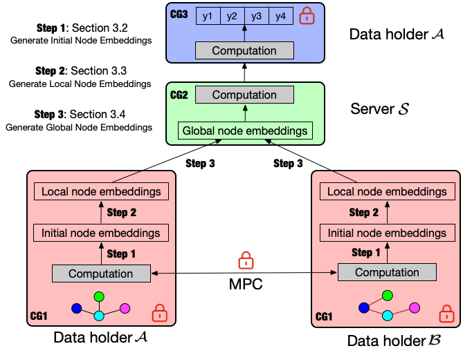
Figure 2: Overview of our proposed VFGNN.

As described in Section 1, for the sake of privacy and efficiency, we design a vertically federated GNN (VFGNN) learning paradigm by splitting the computational graph of GNN into two parts. That is, we keep the private data related computations to data holders for privacy concern, and delegate the non-private data related computations to a semi-honest server for efficiency concern. In the context of GNN, the private data refers to node features, labels, and edges (node relations). To be specific, we divide the computational graph into the following three sub-Computational Graphs (CG), as is shown in Figure 2.

CG1: private feature and edge related computations. The first step of GNN is generating initial node embeddings using node’s private features, e.g., user features in social networks. In vertically data split setting, each data holder has partial node features, as shown in Figure 1. We will present how data holders collaboratively learn initial node embeddings later. In the next step, data holders generate local node embeddings by aggregating multi-hop neighbors’ information using different aggregator functions.

CG2: non-private data related computations. We delegate non-private data related computations to a semi-honest server for efficiency concern. First, the server combines the local node embeddings from data holders with different COMBINE strategies, and obtains the global node embeddings. Next, the server can perform the successive computations using plaintext data. Note that this part has many non-linear computations such as max-pooling and activation functions, which are not cryptographically friendly. For example, existing works approximate the non-linear activations by using either piece-wise functions that need secure comparison protocols Mohassel and Zhang (2017) or high-order polynomials Hardy et al. (2017). Therefore, their accuracy and efficiency are limited. Delegating these plaintext computations to server will not only improve our model accuracy, but also significantly improve our model efficiency, as we will present in experiments. After this, the server gets a final hidden layer ($\textbf{z}_{L}$) and sends it back to the data holder who has label to calculate the prediction, where $L$ is the total number of layers of the deep neural network.

CG3: private label related computations. The data holder who has label can compute prediction using the final hidden layer it receives from the server. For node classification task, the Softmax activation function is used for the output layer Kipf and Welling (2016), which is defined as $\text{softmax}(z_{c})=\frac{1}{Z}\text{exp}(z_{c})$ with $c\in C$ be the node class and $Z=\sum_{c}\text{exp}(z_{c})$.

In the following subsections, we will describe three important components of VFGNN, i.e., initial node embeddings generation in CG1, local node embeddings generation in CG2, and global node embedding generation in CG3.

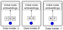
(a) Individually

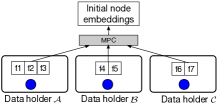
(b) Collaboratively

Figure 3: Methods of generating initial node embeddings.

3.2 Generate Initial Node Embeddings

Initial node embeddings are generated by using node features. Under vertically partitioned data setting, each data holder has partial node features. There are two methods for data holders to generate initial node embeddings, i.e., individually and collaboratively, as shown in Figure 3.

The ‘individually’ method means that data holders generate initial node embeddings using their own node features, individually. For data holder $i\in\mathcal{P}$, this can be done by $\textbf{h}_{0}^{i}={(\textbf{x}^{i})}^{T}\cdot\textbf{W}^{i}$, where $\textbf{x}^{i}$ and $\textbf{W}^{i}$ are node features and weight matrix of data holder $i$. As the example in Figure 3 (a), $\mathcal{A}$, $\mathcal{B}$, and $\mathcal{C}$ generate their initial node embeddings using their own features separately. Although this method is simple and data holders do not need to communicate with each other, it cannot capture the relationship between features of data holders and thus causes information loss.

To solve the shortcoming of ‘individually’ method, we propose a ‘collaboratively’ method. It indicates that data holders generate initial node embeddings using their node features, collaboratively, and meanwhile keep their private features secure. Technically, this can be done by using cryptographic methods such as secret sharing and homomorphic encryption Acar et al. (2018). In this paper, we choose additive secret sharing due to its high efficiency.

3.3 Generate Local Node Embeddings

We generate local node embeddings by using multi-hop neighborhood aggregation on graphs, based on initial node embeddings. Note that, neighborhood aggregation should be done by data holders separately, rather than cooperatively, to protect the private edge information. This is because one may infer the neighboorhoold information of $v$ given the neighborhood aggregation results of $k$-hop ($\textbf{h}^{k}_{v}(i)$) and $k+1$-hop ($\textbf{h}^{k+1}_{v}(i)$), if neighborhood aggregation is done by data holders jointly. For $\forall v\in\mathcal{V}$ at each data holder, neighborhood aggregation is the same as the traditional GNN. Take GraphSAGE Hamilton et al. (2017) for example, it introduces aggregator functions to update hidden embeddings by sampling and aggregating features from a node’s local neighborhood:

$$\small\begin{split}&\textbf{h}_{\mathcal{N}(v)}^{k}\leftarrow\text{AGG}_{k}(\{\textbf{h}_{u}^{k-1},\forall u\in\mathcal{N}(v)\}),\\ &\textbf{h}^{k}_{v}\leftarrow(\textbf{W}^{k}\cdot\text{CONCAT}(\textbf{h}^{k-1}_{v},\textbf{h}_{\mathcal{N}(v)}^{k})),\end{split}$$ (4)

where we follow the same notations as GraphSAGE, and the aggregator functions AGG are of three types, i.e., Mean, LSTM, and Pooling. After it, data holders send local node embeddings to a semi-honest server for combination and further non-private data related computations.

3.4 Generate Global Node Embeddings

The server combines the local node embeddings from data holders and gets global node embeddings. The combination strategy (COMBINE) should be trainable and maintaining high representational capacity, and we design three of them.

Concat. The concat operator can fully preserve local node embeddings learnt from different data holders. That is, Line 14 in Algorithm 2 becomes

$$\small\textbf{h}^{K}_{v}\leftarrow\text{CONCAT}(\textbf{h}^{K}_{v}(1),\textbf{h}^{K}_{v}(2),...,\textbf{h}^{K}_{v}(I)).$$ (5)

Mean. The mean operator takes the elementwise mean of the vectors in $(\{\textbf{h}^{K}_{v}(i),\forall i\in\mathcal{P}\})$, assuming data holders contribute equally to the global node embeddings, i.e.,

$$\small\textbf{h}^{K}_{v}\leftarrow\text{MEAN}(\textbf{h}^{K}_{v}(1)\cup\textbf{h}^{K}_{v}(2)\cup...\cup\textbf{h}^{K}_{v}(I)).$$ (6)

Regression. The above two strategies treat data holders equally. In reality, the local node embeddings from different data holder may contribute diversely to the global node embeddings. We propose a Regression strategy to handle this kind of situation. Let $\boldsymbol{\omega_{i}}$ be the weight vector of local node embeddings from data holder $i\in\mathcal{P}$, then

$$\small\begin{split}&\textbf{h}^{K}_{v}\leftarrow\boldsymbol{\omega_{1}}\odot\textbf{h}^{K}_{v}(1)+\boldsymbol{\omega_{2}}\odot\textbf{h}^{K}_{v}(2)...+\boldsymbol{\omega_{I}}\odot\textbf{h}^{K}_{v}(I),\end{split}$$ (7)

where $\odot$ is element-wise multiplication.

These different combination operators can utilize local node embeddings in diverse ways, and we will empirically study their effects on model performances in experiments.

Algorithm 1 Information publishing mechanisms of data holders to server using differential privacy

Input: Local information of data holders x, dimension of local information $d$, noise multiplier $\sigma$, clipping value $C$.
Output: Differentially private node embeddings.

1:  Scale local information $\mathbf{\bar{x}}=\min(1,{C}/\|\mathbf{x}\|)\mathbf{x};$

2:  Draw i.i.d. samples from $\mathcal{N}(0,\sigma^{2}C^{2})$, which forms a $d$-dimension noise vector $\mathbf{n}$;

3:  # Gaussian Mechanism

4:  Add noise $\mathbf{\tilde{x}}=\mathbf{x}^{K}+\mathbf{n};$

5:  # James-Stein Estimator

6:  Compute James-Stein Estimator $\mathbf{\tilde{x}_{JS}}=\left(1-\frac{(d-2)\sigma^{2}C^{2}}{\|\mathbf{\tilde{x}}\|^{2}}\right)\mathbf{\tilde{x}}$

7:  return $\mathbf{\tilde{x}}$ or $\mathbf{\tilde{x}_{JS}}$.

3.5 Enhancing Privacy by Adopting DP

Data holders directly send the local information, e.g., local node embeddings during forward propagation and gradient update during back propagation, to the server may cause potential information leakage Lyu et al. (2020), and we propose to apply differential privacy to further enhance privacy. In this section, we introduce two DP based data publishing mechanisms, to further enhance the privacy of our proposed VFGNN. Such that with a single entry modification in the local information of data holders, there is a large probability that the server cannot distinguish the difference before or after the modification. We present the two mechanisms, i.e., Gaussian Mechanism and James-Stein Estimator, in Algorithm 1. We have described Gaussian mechanism in Section 2.3, we present James-Stein Estimator as follows.

Theorem 2.

(James-Stein Estimator and its adaptivity Balle and Wang (2018)). Suppose $d$ is the dimension of local information $\mathbf{x}$. When $d\geq 3$, substituting $w$ in $\mathbf{\tilde{x}_{Bayes}}$ with its maximum likelihood estimate under $\mathbf{x}\sim\mathcal{N}(0,w^{2}I)$, $\mathbf{\tilde{x}}|\mathbf{x}\sim\mathcal{N}(\mathbf{x},\sigma^{2}C^{2}I)$, and $\mathbf{\tilde{x}_{Bayes}}=argmin_{\mathbf{\tilde{x}}}\|\mathbf{\tilde{x}}-\mathbf{x}\|^{2}$ produces James-Stein Estimator $\mathbf{\tilde{x}_{JS}}=\left(1-\frac{(d-2)\sigma^{2}C^{2}}{\|\mathbf{\tilde{x}}\|^{2}}\right)\mathbf{\tilde{x}}.$ Moreover, it has an Mean Squared Error (MSE) of

$$\small E[\|\mathbf{\tilde{x}_{JS}}-\mathbf{x}\|^{2}]=d\sigma^{2}\left(1-\frac{(d-2)^{2}}{d^{2}}\frac{\sigma^{2}C^{2}}{w^{2}+\sigma^{2}C^{2}}\right).$$ (8)

The MSE of Gaussian Mechanism $\mathbf{\tilde{x}}$ to exact $\mathbf{x}$ is $E\|\mathbf{\tilde{x}}-\mathbf{x}\|^{2}=d\sigma^{2}C^{2}$, while the MSE of James-Stein Estimator is reduced with a factor of $(1-\frac{(d-2)^{2}}{d^{2}}\frac{\sigma^{2}C^{2}}{w^{2}+\sigma^{2}C^{2}})$. Both methods preserve $(\epsilon,\delta)$-DP while James-Stein estimator shows reductions in MSE, thus improves utility. By the definition of Gaussian mechanism (Definition 3), we have the privacy loss for both information publishing mechanisms in Algorithm 1. By combining it with Moment Accountant (MA) Abadi et al. (2016), we present the overall privacy for $T$ iterations.

Theorem 3.

Suppose each iteration of Algorithm 1 is $(\epsilon,\delta)-$DP. There exist constants $c_{1}$ and $c_{2}$ so that given the sampling probability $q$ and the number of iterations $T$, and $\epsilon<c_{1}q\sqrt{T}$, Algorithm 1 over $T$ iteration is $(\epsilon^{\prime},\delta)-$DP, with $\epsilon^{\prime}=c_{2}q\sqrt{T}\epsilon$.

Proof.

By Definition 3 and Theorem 1, to ensure one iteration $(\epsilon,\delta)-$DP, we set $\sigma=\frac{\sqrt{2\ln(1.25/\delta)}}{\epsilon}$. By Theorem 1 in  Abadi et al. (2016), with $\sigma=\frac{\sqrt{2\ln(1.25/\delta)}}{\epsilon}$ and the appropriate choice of $\epsilon,q,T$, such that $\epsilon<c_{1}q\sqrt{T}$, the privacy loss over $T$ iterations is $\epsilon^{\prime}=\frac{c_{1}q\sqrt{T\log(1/\delta)}}{\sigma}=c_{2}q\sqrt{T}\epsilon.$ ∎

Algorithm 2 Privacy-preserving GraphSAGE for node label prediction (forward propagation)

Input: Data holder $\forall i\in\mathcal{P}$; Graph $\mathcal{G}(\mathcal{V},\mathcal{E}^{i})$ and node features {$\textbf{x}^{i}_{v},\forall v\in\mathcal{V}$}; depth $K$; aggregator functions AGG${}_{k},\forall k\in\{1,...,K\}$; weight matrices $\textbf{W}_{i}^{k},\forall k\in\{1,...,K\}$; max layer $L$; weight matrices $\textbf{W}_{l},\forall l\in\{0,...,L\}$; non-linearity $\sigma$; neighborhood functions $\mathcal{N}^{i}:v\rightarrow 2^{\mathcal{V}}$; node labels on data holder $p\in\mathcal{P}$ and $c\in C$
Output: Node label predictions {$\hat{y}_{vc},\forall v\in\mathcal{V},\forall c\in C$}

1:  # CG1: private feature and edge related computations

2:  Data holders: jointly calculate initial node embeddings $\textbf{h}_{v}^{0}(i)\leftarrow\textbf{x}^{i}_{v},\forall i\in\mathcal{P},\forall v\in\mathcal{V}$

3:  for $i\in\mathcal{P}$ in parallel do

4:     for $k=1$ to $K$ do

5:        for $v\in\mathcal{V}$ do

6:           Data holder: calculates $\textbf{h}_{\mathcal{N}(v)}^{k}(i)\leftarrow$ AGG${}_{k}(\{\textbf{h}_{u}^{k-1}(i),\forall u\in\mathcal{N}^{i}(v)\})$

7:        end for

8:        Data holder: calculates $\textbf{h}^{k}_{v}(i)\leftarrow\sigma(\textbf{W}_{i}^{k}\cdot$ CONCAT $(\textbf{h}^{k-1}_{v}(i),\textbf{h}_{\mathcal{N}(v)}^{k}(i))$

9:     end for

10:     Data holder: calculates local node embeddings $\textbf{h}^{K}_{v}(i)\leftarrow\textbf{h}^{K}_{v}(i)/||\textbf{h}^{K}_{v}(i)||_{2},\forall v\in\mathcal{V}$ and sends (publishes) it to server using differential privacy

11:  end for

12:  # CG2: non-private data related computations

13:  for $v\in\mathcal{V}$ do

14:     Server: combines the local node embeddings from data holders $\textbf{h}^{K}_{v}=$ COMBINE $(\{\textbf{h}^{K}_{v}(i),\forall i\in\mathcal{P}\})$

15:     Server: forward propagation based on the global node embeddings $\textbf{z}_{L}=\sigma(\textbf{W}_{L-1}\cdot\sigma(...\sigma(\textbf{W}_{0}\cdot\textbf{h}^{K}_{v})))$

16:     Server: sends $\textbf{z}_{L}$ to data holder $p$

17:  end for

18:  # CG3: private label related computations

19:  Data holder $p$: makes prediction by $\hat{y}_{vc}\leftarrow\text{softmax}(\textbf{W}_{L}\cdot\textbf{z}_{L}),\forall v\in\mathcal{V},\forall c\in C$

3.6 Putting Together

By combining CG1-CG3 and the key components described above, we complete the forward propagation of VFGNN. To describe the procedures in details, without loss of generality, we take GraphSAGE Hamilton et al. (2017) for example and present its forward propagation process in Algorithm 2. VFGNN can be learnt by gradient descent through minimizing the cross-entropy error over all labeled training examples.

Specifically, the model weights of VFGNN are in four parts. (1) The weights for the initial node embeddings, i.e., $\langle\textbf{W}\rangle_{i},\forall i\in\mathcal{P}$, that are secretly shared by data holders, (2) the weights for neighborhoold aggregation on graphs, i.e., $\textbf{W}_{i}^{k}$, that are also kept by data holders, (3) the weights for the hidden layers of deep neural networks, i.e., $\textbf{W}_{l},0\leq l<L$, that are hold by server, (4) and the weights for the output layer of deep neural networks, i.e., $\textbf{W}_{L}$, that are hold by the data holder who has label. As can be seen, in VFGNN, both private data and model are hold by data holders themselves, thus data privacy can be better guaranteed.

4 Experiments

We conduct experiments to answer the following questions. Q1: whether VFGNN outperforms the GNN models that are trained on the isolated data. Q2: how does VFGNN behave comparing with the traditional insecure model trained on the plaintext mixed data. Q3: how does VFGNN perform comparing with the naive solution in Section 1. Q4: are our proposed combination strategies effective to VFGNN. Q5: what is the effect of the number of data holders on VFGNN. Q6: what is the effect of differential privacy on VFGNN.

4.1 Experimental Setup

Datasets. We use four benchmark datasets, i.e., Cora, Pubmed, Citeseer Sen et al. (2008), and arXiv Hu et al. (2020). We use exactly the same dataset partition of training, validate, and test following the prior work Kipf and Welling (2016); Hu et al. (2020). Besides, in data isolated GNN setting, both node features and edges are hold by different parties. For all the experiments, we use five-fold cross validation and adopt average accuracy as the evaluation metric.

Dataset	#Node	#Edge	#Features	#Classes
Cora	2,708	5,429	1,433	7
Pubmed	19,717	44,338	500	3
Citeseer	3,327	4,732	3,703	6
arXiv	169,343	2,315,598	128	40

Table 1: Dataset statistics.

Comparison methods. We compare VFGNN with GraphSAGE models Hamilton et al. (2017) that are trained using isolated data and mixed plaintext data to answer Q1 and Q2. We also compare VFGNN with the naive solution described in Section 1 to answer Q3. To answer Q4, we vary the proportion of the data (features and edges) hold by $\mathcal{A}$ and $\mathcal{B}$, and change VFGNN with different combination strategies. We vary the number of data holders in VFGNN to answer Q5, and vary the parameters of differential privacy to answer Q6. For all these models, we choose Mean operator as the aggregator function.

Parameter settings. For all the models, we use TanH as the active function of neighbor propagation, and Sigmoid as the active function of hidden layers. For the deep neural network on server, we set the dropout rate to 0.5 and network structure as ($d$, $d$, $|C|$), where $d\in\{32,64,128\}$ is the dimension of node embeddings and $|C|$ the nubmer of classes. We vary $\epsilon\in\{1,2,4,8,16,32,64,\infty\}$, set $\delta=1e^{-4}$ and the clip value $C=1$ to study the effects of differential privacy on our model. Since we have many comparison and ablation models, and they achieve the best performance with different parameters, we cannot report all the best parameters. Instead, we report the range of the best parameters. We vary the propagation depth $K\in\{2,3,4,5\}$, L2 regularization in $\{10^{-2}-10^{-4}\}$, and learning rate in $\{10^{-2}-10^{-3}\}$. We tune parameters based on the validate dataset and evaluate model performance on the test dataset.

4.2 Comparison Results and Analysis

To answer Q1-Q3, we assume there are two data holders ($\mathcal{A}$ and $\mathcal{B}$) who have equal number of node features and edges, i.e., the proportion of data held by $\mathcal{A}$ and $\mathcal{B}$ is 5:5, and compare our models with GraphSAGEs that are trained on isolated data individually and on mixed plaintext data. We also set $\epsilon=\infty$ during comparison and will study its effects later. We summarize the results in Table 2, where VFGNN_C, VFGNN_M, and VFGNN_R denote VFGNN with Concat, Mean, and Regression combination strategies.

Result1: answer to Q1. We first compare VFGNNs with the GraphSAGEs that are trained on isolated feature and edge data, i.e., GraphSAGE_A and GraphSAGE_B. From Table 2, we find that, VFGNNs with different combination strategies significantly outperforms GraphSAGE_A and GraphSAGE_B on all the three datasets. Take Citeseer for example, our VFGNN_R improves GraphSAGE_A and GraphSAGE_B by as high as 28.10% and 51.64%, in terms of accuracy.

Analysis of Result1. The reason of result1 is straightforward. GraphSAGE_A and GraphSAGE_B can only use partial feature and edge information held by $\mathcal{A}$ and $\mathcal{B}$. In contrast, VFGNNs provide a solution for $\mathcal{A}$ and $\mathcal{B}$ to jointly train GNNs without compromising their own data. By doing this, VFGNNs can use the information from the data of both $\mathcal{A}$ and $\mathcal{B}$ simultaneously, and therefore achieve better performance.

Dataset	Cora	Pubmed	Citeseer	arXiv
GraphSAGEA	0.611	0.672	0.541	0.471
GraphSAGEB	0.606	0.703	0.457	0.482
VFGNN_C	0.790	0.774	0.685	0.513
VFGNN_M	0.809	0.781	0.695	0.522
VFGNN_R	0.802	0.782	0.693	0.518
GraphSAGEA+B	0.815	0.791	0.700	0.529

Table 2: Comparison results on three datasets (Q1 and Q2).

Result2: answer to Q2. We then compare VFGNNs with GraphSAGE that is trained on the mixed plaintext data, i.e., GraphSAGE_A+B. It can be seen from Table 2 that VFGNNs have comparable performance with GraphSAGE_A+B, e.g., 0.8090 vs. 0.8150 on Cora dataset and 0.6950 vs. 0.7001 on Citeseer dataset.

Analysis of Result2. It is easy to explain why our proposal has comparable performance with the model that are trained on the mixed plaintext data. First, we propose a secret sharing based protocol for $\mathcal{A}$ and $\mathcal{B}$ to generate the initial node embeddings from their node features, which are the same as those generated by using mixed plaintext features. Second, although $\mathcal{A}$ and $\mathcal{B}$ generate local node embeddings by using their own edge data to do neighbor aggregation separately (for security concern), we propose different combination strategies to combine their local node embeddings. Eventually, the edge information from both $\mathcal{A}$ and $\mathcal{B}$ is used for training the classification model. Therefore, VFGNN achieves comparable performance with GraphSAGE_A+B.

Result3: answer to Q3. In VFGNN, we delegate the non-private data related computations to server. One would be curious about what if these computations are also performed by data holders using existing secure neural network protocols, i.e., SecureML Mohassel and Zhang (2017). To answer this question, we compare VFGNN with the secure GNN model that is implemented using SecureML, which we call as SecureGNN, where we use 3-degree Taylor expansion to approximate TanH and Sigmoid. The accuracy and running time per epoch (in seconds) of VFGNN vs. SecureGNN on Pubmed are 0.8090 vs. 0.7970 and 18.65 vs. 166.81, respectively, where we use local area network.

Analysis of Result3. From the above comparison results, we find that our proposed VFGNN learning paradigm not only achieves better accuracy, but also has much better efficiency. This is because the non-private data related computations involve many non-linear functions that are not cryptographically friendly, which have to be approximately calculated using time-consuming MPC techniques in SecureML.

Model	VFGNN_C	VFGNN_M	VFGNN_R
Prop.=9:1	0.809	0.805	0.809
Prop.=8:2	0.802	0.796	0.807
Prop.=7:3	0.793	0.793	0.803

Table 3: Comparison of combination operators on Cora by varying the proportion of data hold by $\mathcal{A}$ and $\mathcal{B}$ (Q4).

No. of DH	VFGNN_C	VFGNN_M	VFGNN_R
2	0.790	0.809	0.802
3	0.749	0.774	0.760
4	0.712	0.733	0.722

Table 4: Comparison results on Cora by varying the number of data holders (Q5).

4.3 Ablation Study

We now study the effects of different combination operators and different number of data holders on VFGNN.

Result4: answer to Q4. Different combination operators can utilize local node embeddings in diverse ways and make our proposed VFGNN adaptable to different scenarios, we study this by varying the proportion (Prop.) of data (node features and edges) hold by $\mathcal{A}$ and $\mathcal{B}$ in $\{9\colon 1,8\colon 2,7\colon 3\}$. The results on Cora dataset are shown in Table 3.

Analysis of Result4. From Table 3, we find that with the proportion of data hold by $\mathcal{A}$ and $\mathcal{B}$ being even, i.e., from $\{9\colon 1\}$ to $\{7\colon 3\}$, the performances of most strategies tend to decrease. This is because the neighbor aggregation is done by data holders individually, and with a bigger proportion of data hold by a single holder, it is easier for this party to generate better local node embeddings. Moreover, we also find that Mean operator works well when data are evenly split, and Regression operator is good at handling the situations where data holders have different quatity of data, since it treats the local node embeddings from each data holder differently, and assigns weights to them intelligently.

Result5: answer to Q5. We vary the number of data holders in {2, 3, 4} and study the performance of VFGNN. We report the results in Table 4, where we use the Cora dataset and assume data holders have even feature and edge data.

Analysis of Result5. From Table 4, we find that, as the number of data holders increases, the accuracy of all the models decreases. This is because the neighborhood aggregation in VFGNN is done by each holder individually for privacy concern, and each data holder will have less edge data when there are more data holders, since they split the original edge information evenly. Therefore, when more participants are involved, more information will be lost during the neighborhood aggregation procedure.

$\epsilon$	4	8	16	32	64
Gaussian	0.502	0.702	0.772	0.789	0.794
James-Stein	0.510	0.706	0.781	0.799	0.804

Table 5: Effect of DP on VFGNN using Cora dataset (Q6).

Result6: answer to Q6. We present the privacy loss of each iteration in Table 5 and the over all privacy in Theorem 3. We vary $\epsilon$ and set $\delta=1e^{-4}$ to study the effects of DP on VFGNN. We report the results in Table 5, where we use Cora dataset, use MEAN as the combination operator, and assume data holders have even feature and edge data.

Analysis of Result6. From Table 5, we can see that the accuracy of VFGNN increases with $\epsilon$. In other words, there is a trade-off between accuracy and privacy. The smaller $\epsilon$, the more noise will be added into the local node embeddings, which causes stronger privacy guarantee but lower accuracy. We also find James-Stein estimator consistently works better than Gaussian mechanism, since it can reduce MSE, as we have analyzed in Section 3.5.

5 Conclusion

We propose VFGNN, a vertically federated GNN learning paradigm for privacy-preserving node classification task. We finish this by splitting the computation graph of GNN. We leave the private data related computations on data holders and delegate the rest computations to a server. Experiments on real world datasets demonstrate that our model significantly outperforms the GNNs by using the isolated data and has comparable performance with the traditional GNN by using the mixed plaintext data insecurely.

Appendix A Multiplication of Secret Sharing

Existing research on secret sharing multiplication protocol is mainly based on Beaver’s triplet technique Beaver [1991]. Specifically, to multiply two secretly shared values $\langle a\rangle$ and $\langle b\rangle$ between two parties $\mathcal{P}_{0}$ and $\mathcal{P}_{1}$, they first need to collaboratively choose a shared triple $\langle u\rangle$, $\langle w\rangle$, and $\langle z\rangle$, where $u,w$ are uniformly random values in $\mathds{Z}_{2^{\ell}}$ and $z=uw$ mod $2^{\ell}$. They then locally compute $\langle e\rangle_{i}=\langle a\rangle_{i}-\langle u\rangle_{i}$ and $\langle f\rangle_{i}=\langle b\rangle_{i}-\langle w\rangle_{i}$, where $i\in\{0,1\}$. Next, they run $\textbf{Rec}(\langle e\rangle_{0},\langle e\rangle_{1})$ and $\textbf{Rec}(\langle f\rangle_{0},\langle f\rangle_{1})$. Finally, $\mathcal{P}_{i}$ gets $\langle c\rangle_{i}=-i\cdot e\cdot f+f\cdot\langle a\rangle_{i}+e\cdot\langle b\rangle_{i}+\langle z\rangle_{i}$ as a share of the multiplication result, such that $\langle a\rangle\langle b\rangle=\langle c\rangle_{0}+\langle c\rangle_{1}$. It is easy to vectorize the addition and multiplication protocols under secret sharing setting. The above protocols work in finite field, and we adopt fixed-point representation to approximate decimal arithmetics efficiently Mohassel and Zhang [2017].

Appendix B Related Work in Details

We review three kinds of existing Privacy-Preserving Neural Network (PPNN) models, including GNN models.

PPNN based on cryptographic methods. These methods mainly use cryptographic techniques, e.g., secret sharing and homomorphic encryption, to build approximated neural networks models Mohassel and Zhang [2017]; Wagh et al. [2019], since the nonlinear active functions are not cryptographically computable. Cryptograph based neural network models are difficult to scale to deep networks and large datasets due to its high communication and computation complexities. In this paper, we use cryptographic techniques for data holders to calculate the initial node embeddings securely.

PPNN based on federated learning. The privacy issues in machine learning has boosted the development of federated learning. To date, federated neural networks have been extensively studied Konečnỳ et al. [2016]; Bonawitz et al. [2019] and applied into real-world scenarios Li et al. [2020]. There are also several work on federated GNN when data are horizontally partitioned Zheng et al. [2021]; Wu et al. [2021]. However, a mature solution for federated GNN models under vertically partitioned data is still missing. In this paper, we fill this gap by proposing VFGNN.

PPNN based on split computation graph. These methods split the computation graph of neural networks into two parts, and let data holders calculate the private data related computations individually and get a hidden layer, and then let a server makes the rest computations Vepakomma et al. [2018]; Chi et al. [2018]; Osia et al. [2019]; Gu et al. [2018]; Zheng et al. [2020]. Our model differs from them in mainly two aspects. First, we train a GNN rather than a neural network. Seconds, we use cryptographic techniques for data holders to calculate the initial node embeddings collaboratively rather than compute them based on their plaintext data individually.

Algorithm 3 Data holders $\mathcal{P}$ securely generate the initial node embeddings using secret sharing

Input: {$\textbf{x}^{i}_{v}\in\mathds{Z}_{2^{\ell}},\forall v\in\mathcal{V},\forall i\in\mathcal{P}$}, and $\textbf{x}^{i}$ for short
Output: The share of initial node embeddings for each data holder $i$ {$\textbf{h}_{v}^{0}(i),i\in\mathcal{P},\forall v\in\mathcal{V}$}

1:  for $\mathcal{P}_{i}\in\mathcal{P}$ in parallel do

2:     $\mathcal{P}_{i}$ randomly initializes $\langle\textbf{W}\rangle_{i}$

3:     $\mathcal{P}_{i}$ locally generates $\left\{\left\langle\textbf{x}^{i}\right\rangle_{j}\right\}_{j\in\mathcal{P}}$

4:     $\mathcal{P}_{i}$ distributes $\left\{\left\langle\textbf{x}^{i}\right\rangle_{j}\right\}_{j\neq i}$ to others

5:     $\mathcal{P}_{i}$ concats $\left\{\left\langle\textbf{x}^{k}\right\rangle_{j}\right\}_{j\in\mathcal{P}}$ and get $\left\langle\textbf{x}\right\rangle_{i}$

6:     $\mathcal{P}_{i}$ locally calculates $\left\langle\textbf{x}\right\rangle_{i}^{T}\cdot\langle\textbf{W}\rangle_{i}$ as $i$-share

7:  end for

8:  for $\mathcal{P}_{j}\in\mathcal{P}$ and $j\neq i$ do

9:     $\mathcal{P}_{i}$ and $\mathcal{P}_{j}$ calculate $i$-share $\left\langle\left\langle\textbf{x}\right\rangle_{i}^{T}\cdot\langle\textbf{W}\rangle_{j}\right\rangle_{i}$ and $j$-share $\left\langle\left\langle\textbf{x}\right\rangle_{i}^{T}\cdot\langle\textbf{W}\rangle_{j}\right\rangle_{j}$ using secret sharing

10:     $\mathcal{P}_{i}$ and $\mathcal{P}_{j}$ calculate $i$-share $\left\langle\left\langle\textbf{x}\right\rangle_{j}^{T}\cdot\langle\textbf{W}\rangle_{i}\right\rangle_{i}$ and $j$-share $\left\langle\left\langle\textbf{x}\right\rangle_{j}^{T}\cdot\langle\textbf{W}\rangle_{i}\right\rangle_{j}$ using secret sharing

11:  end for

12:  for $\mathcal{P}_{i}\in\mathcal{P}$ in parallel do

13:     $\mathcal{P}_{i}$ locally calculates the summation of all $i$-shares, denoted as $\left\langle\textbf{h}_{v}^{0}\right\rangle_{i}=\left\langle\textbf{x}^{T}\cdot\textbf{w}\right\rangle_{i}$

14:     $\mathcal{P}_{i}$ sends $\left\langle\textbf{h}_{v}^{0}\right\rangle_{i}$ to $\mathcal{P}_{j}$, $\forall j\in\mathcal{P},j\neq i$

15:     $\mathcal{P}_{i}$ reconstructs $\textbf{h}_{v}^{0}$, denote as $\textbf{h}_{v}^{0}(i)$

16:  end for

17:  return $\textbf{h}_{v}^{0}(i)$ for each data holder $i\in\mathcal{P}$

Appendix C Algorithm of Generating Initial Node Embeddings

We summarize the algorithm of generating initial node embeddings in Algorithm 1. Traditionally, the initial node embeddings can be generated by $\textbf{h}_{0}=\textbf{x}^{T}\cdot\textbf{W}$, where x is node features and W is weight matrix. When features are vertically partitioned, we calculate initial node embeddings as follows. First, we secretly share x among data holders (Lines 3-4). Then, data holders concat their received shares in order (Line 5). After it, we calculate $\textbf{x}^{T}\cdot\textbf{W}$ following distributive law (Lines 8-11). Take two data holders for example, $\textbf{x}^{T}\cdot\textbf{W}=(\left\langle\textbf{x}\right\rangle_{1}+\left\langle\textbf{x}\right\rangle_{2})\cdot(\left\langle\textbf{W}\right\rangle_{1}+\left\langle\textbf{W}\right\rangle_{2})=\left\langle\textbf{x}\right\rangle_{1}\cdot\left\langle\textbf{W}\right\rangle_{1}$ $+\left\langle\textbf{x}\right\rangle_{1}\cdot\left\langle\textbf{W}\right\rangle_{2}+\left\langle\textbf{x}\right\rangle_{2}\cdot\left\langle\textbf{W}\right\rangle_{1}+\left\langle\textbf{x}\right\rangle_{2}\cdot\left\langle\textbf{W}\right\rangle_{2}$. Finally, data holders reconstruct $\textbf{x}^{T}\cdot\textbf{W}$ by summing over all the shares (Lines 12-16).

References

- Abadi et al. [2016] Martin Abadi, Andy Chu, Ian Goodfellow, H Brendan McMahan, Ilya Mironov, Kunal Talwar, and Li Zhang. Deep learning with differential privacy. In CCS, pages 308–318. ACM, 2016.
- Acar et al. [2018] Abbas Acar, Hidayet Aksu, A Selcuk Uluagac, and Mauro Conti. A survey on homomorphic encryption schemes: Theory and implementation. ACM Computing Surveys (CSUR), 51(4):79, 2018.
- Balle and Wang [2018] Borja Balle and Yu-Xiang Wang. Improving the gaussian mechanism for differential privacy: Analytical calibration and optimal denoising. arXiv preprint arXiv:1805.06530, 2018.
- Beaver [1991] Donald Beaver. Efficient multiparty protocols using circuit randomization. In Annual International Cryptology Conference, pages 420–432. Springer, 1991.
- Bonawitz et al. [2019] Keith Bonawitz, Hubert Eichner, Wolfgang Grieskamp, Dzmitry Huba, Alex Ingerman, Vladimir Ivanov, Chloe Kiddon, Jakub Konečnỳ, Stefano Mazzocchi, H Brendan McMahan, et al. Towards federated learning at scale: System design. arXiv preprint arXiv:1902.01046, 2019.
- Chen et al. [2021] Chaochao Chen, Jun Zhou, Li Wang, Xibin Wu, Wenjing Fang, Jin Tan, Lei Wang, Alex X. Liu, Hao Wang, and Cheng Hong. When homomorphic encryption marries secret sharing: Secure large-scale sparse logistic regression and applications in risk control. In SIGKDD, pages 2652–2662. ACM, 2021.
- Chi et al. [2018] Jianfeng Chi, Emmanuel Owusu, Xuwang Yin, Tong Yu, William Chan, Patrick Tague, and Yuan Tian. Privacy partitioning: Protecting user data during the deep learning inference phase. arXiv preprint arXiv:1812.02863, 2018.
- Costan and Devadas [2016] Victor Costan and Srinivas Devadas. Intel sgx explained. IACR Cryptology ePrint Archive, 2016(086):1–118, 2016.
- Dwork et al. [2014] Cynthia Dwork, Aaron Roth, et al. The algorithmic foundations of differential privacy. Foundations and Trends in Theoretical Computer Science, 9(3-4):211–407, 2014.
- Fang et al. [2021] Wenjing Fang, Derun Zhao, Jin Tan, Chaochao Chen, Chaofan Yu, Li Wang, Lei Wang, Jun Zhou, and Benyu Zhang. Large-scale secure XGB for vertical federated learning. In CIKM, pages 443–452. ACM, 2021.
- Gu et al. [2018] Zhongshu Gu, Heqing Huang, Jialong Zhang, Dong Su, Ankita Lamba, Dimitrios Pendarakis, and Ian Molloy. Securing input data of deep learning inference systems via partitioned enclave execution. arXiv preprint arXiv:1807.00969, 2018.
- Hamilton et al. [2017] Will Hamilton, Zhitao Ying, and Jure Leskovec. Inductive representation learning on large graphs. In NeurIPS, pages 1024–1034, 2017.
- Hardy et al. [2017] Stephen Hardy, Wilko Henecka, Hamish Ivey-Law, Richard Nock, Giorgio Patrini, Guillaume Smith, and Brian Thorne. Private federated learning on vertically partitioned data via entity resolution and additively homomorphic encryption. arXiv preprint arXiv:1711.10677, 2017.
- He et al. [2020] Xinlei He, Jinyuan Jia, Michael Backes, Neil Zhenqiang Gong, and Yang Zhang. Stealing links from graph neural networks. arXiv preprint arXiv:2005.02131, 2020.
- Hu et al. [2020] Weihua Hu, Matthias Fey, Marinka Zitnik, Yuxiao Dong, Hongyu Ren, Bowen Liu, Michele Catasta, and Jure Leskovec. Open graph benchmark: Datasets for machine learning on graphs. arXiv preprint arXiv:2005.00687, 2020.
- Kipf and Welling [2016] Thomas N Kipf and Max Welling. Semi-supervised classification with graph convolutional networks. arXiv preprint arXiv:1609.02907, 2016.
- Konečnỳ et al. [2016] Jakub Konečnỳ, H Brendan McMahan, Felix X Yu, Peter Richtárik, Ananda Theertha Suresh, and Dave Bacon. Federated learning: Strategies for improving communication efficiency. arXiv preprint arXiv:1610.05492, 2016.
- Li et al. [2020] Li Li, Yuxi Fan, Mike Tse, and Kuo-Yi Lin. A review of applications in federated learning. Computers & Industrial Engineering, page 106854, 2020.
- Lyu et al. [2020] Lingjuan Lyu, Han Yu, Jun Zhao, and Qiang Yang. Threats to federated learning. In Federated Learning, pages 3–16. Springer, 2020.
- Mohassel and Zhang [2017] Payman Mohassel and Yupeng Zhang. Secureml: A system for scalable privacy-preserving machine learning. In S&P, pages 19–38, 2017.
- Osia et al. [2019] Seyed Ali Osia, Ali Shahin Shamsabadi, Ali Taheri, Kleomenis Katevas, Sina Sajadmanesh, Hamid R Rabiee, Nicholas D Lane, and Hamed Haddadi. A hybrid deep learning architecture for privacy-preserving mobile analytics. arXiv preprint arXiv:1703.02952, 2019.
- Sajadmanesh and Gatica-Perez [2020] Sina Sajadmanesh and Daniel Gatica-Perez. Locally private graph neural networks. CoRR abs/2006.05535, 12, 2020.
- Sen et al. [2008] Prithviraj Sen, Galileo Namata, Mustafa Bilgic, Lise Getoor, Brian Galligher, and Tina Eliassi-Rad. Collective classification in network data. AI magazine, 29(3):93–93, 2008.
- Shamir [1979] Adi Shamir. How to share a secret. Communications of the ACM, 22(11):612–613, 1979.
- Veličković et al. [2017] Petar Veličković, Guillem Cucurull, Arantxa Casanova, Adriana Romero, Pietro Lio, and Yoshua Bengio. Graph attention networks. arXiv preprint arXiv:1710.10903, 2017.
- Vepakomma et al. [2018] Praneeth Vepakomma, Otkrist Gupta, Tristan Swedish, and Ramesh Raskar. Split learning for health: Distributed deep learning without sharing raw patient data. arXiv preprint arXiv:1812.00564, 2018.
- Wagh et al. [2019] Sameer Wagh, Divya Gupta, and Nishanth Chandran. Securenn: 3-party secure computation for neural network training. PETs, 1:24, 2019.
- Wu et al. [2019] Zonghan Wu, Shirui Pan, Fengwen Chen, Guodong Long, Chengqi Zhang, and Philip S Yu. A comprehensive survey on graph neural networks. arXiv preprint arXiv:1901.00596, 2019.
- Wu et al. [2021] Chuhan Wu, Fangzhao Wu, Yang Cao, Yongfeng Huang, and Xing Xie. Fedgnn: Federated graph neural network for privacy-preserving recommendation. arXiv preprint arXiv:2102.04925, 2021.
- Zheng et al. [2020] Longfei Zheng, Chaochao Chen, Yingting Liu, Bingzhe Wu, Xibin Wu, Li Wang, Lei Wang, Jun Zhou, and Shuang Yang. Industrial scale privacy preserving deep neural network. arXiv preprint arXiv:2003.05198, 2020.
- Zheng et al. [2021] Longfei Zheng, Jun Zhou, Chaochao Chen, Bingzhe Wu, Li Wang, and Benyu Zhang. Asfgnn: Automated separated-federated graph neural network. PPNA, pages 1–13, 2021.