Interplay between degree and Boolean rules in the stability of Boolean networks

Abstract

Empirical evidence has revealed that biological regulatory systems are controlled by high-level coordination between topology and Boolean rules. In this study, we study the joint effects of degree and Boolean functions on the stability of Boolean networks. To elucidate these effects, we focus on i) the correlation between the sensitivity of Boolean variables and the degree, and ii) the coupling between canalizing inputs and degree. We find that negatively correlated sensitivity with respect to local degree enhances the stability of Boolean networks against external perturbations. We also demonstrate that the effects of canalizing inputs can be amplified when they coordinate with high in-degree nodes. Numerical simulations confirm the accuracy of our analytical predictions at both the node and network levels.

How to predict and assess the stability of the Boolean networks is an important problem of much interest. Recently, an exhaustive search of real-world biological circuits has revealed the high-level coordination between network topology and Boolean variables. However, the role of the correlations between structural and dynamic properties is still not fully understood. Here, we study the stability of random Boolean networks with intertwined the degree and Boolean functions. We demonstrate that analysis based on the naive mean-field approach may fail to predict dynamical consequences in Boolean networks with intertwined structural and functional properties, which are often observed in real-world biological systems.

I Introduction

The random Boolean network proposed by Kauffman in $1969$ kauffman1969 has been widely used in physics, biology, and computer science for modeling biological regulatory systems in an abstract manner karlebach2008 ; albert2008 ; li2004 ; thomas2001 ; shmulevich2002 . Many functions in living systems can be modeled by Boolean networks, including genetic regulation kauffman1969 ; li2004 ; thomas2001 , neural firing rosin2013 , and social activity sayama2013 . The dynamical patterns of Boolean networks fall into two phases, namely stable and unstable (chaotic) phases. In a stable phase, most nodes rapidly reach a steady state and remain unchanged. In contrast, in an unstable phase most nodes change their states in a chaotic manner. It has been suggested that many biological regulatory systems ranging from genetic systems to neural systems tend to hover near the borderline between these two phases, achieving both stability and evolvability kauffmanbook ; munoz2018 ; krotov2014 . Empirical evidence supports the hypothesis that biological networks remain near criticality kauffmanbook ; daniels2018 , especially for knockout experiments for single genes in Saccharomyces cerevisiae serra2004 and gene expression dynamics in macrophages nykter2008 .

Theoretical predictions regarding the dynamics of Boolean networks are based on stability against perturbations derrida1986 ; luque1997 . While damage caused by perturbations dies out quickly in a stable phase, it can spread through an entire system in an unstable phase. Pioneering research on the theoretical prediction of the stability of random Boolean networks has revealed that the mean degree $\langle k\rangle$ of a network and the mean bias $\langle p\rangle$ of Boolean functions typically determine the location of criticality derrida1986 ; luque1997 . Since then, many studies have attempted to assess the effects of structural and dynamical features, including scale-free structures aldana2002 ; lee2008 , noise peixoto2009 ; villegas2016 , multi-level interactions cozzo2012 , asynchronous updates klemm2005 , continuous dynamics ghanbarnejad2011 , veto functions ebadi2014 , bipartite interactions lee2012 , knockout boldhaus2010 ; wang2018 , adaptive dynamics goudarzi2012 , and canalizing functions moreira2005 .

Recently, an exhaustive search of real-world networks revealed that biological regulatory circuits achieve stable and adaptive functionality based on the interplay between logical variables and causal structures daniels2018 . To be specific, anti-correlated sensitivity to the local degree of nodes and abundant canalizing functions were observed in the real-world biological networks across diverse regulatory systems daniels2018 ; moreira2005 . Therefore, it is expected that real-world biological networks achieve near-critical behavior in a distinguished way than random Boolean networks without any correlation between Boolean rules and topology. There have been several attempts to study the role of the correlations between structural and dynamic properties in Boolean networks shmulevich2004 ; squires2014 ; pomerance2009 , but this role is still not fully understood, particularly for the correlations between node degree and Boolean functions.

In this study, we analyze the stability of a random Boolean network incorporating interplay between network topology and Boolean variables. Specifically, we aim to assess the effects of the correlation between local node degree and Boolean functions in terms of sensitivity shmulevich2004 ; squires2014 and canalizing inputs moreira2005 . In this paper, we elucidate the role of the coupling between local topology and Boolean rules in promoting the stability of Boolean networks. Specifically, we demonstrate that negatively correlated sensitivity to degree enhances the stability of Boolean networks. Additionally we find that coordination between high-degree nodes and canalizing inputs can enhance stability. Numerical simulations are conducted to verify our analytical predictions, revealing excellent agreement.

II Theory

II.1 Semi-annealed approximation

A Boolean network consists of a set of nodes whose states are binary (i.e., on or off). Directed links between nodes in a Boolean network represent the regulatory interactions. We denote in- and out-degrees of node $i$ as $k_{i}^{in}$ and $k_{i}^{out}$. We assign the bias $p_{i}$ for node $i$ which indicates the probability of a Boolean function to return on state. A Boolean function or truth table for every combination (total of $2^{k_{i}^{in}}$ combinations) of inputs is assigned according to the bias $p_{i}$. Here we consider a single fixed network and randomly reassigning Boolean inputs to all nodes at each time step, so called semi-annealed approximation.

Starting from an initial state selected at random, the state of each node is updated synchronously according to its Boolean function and input signals. After a transient period, the dynamics of the Boolean network eventually arrives at a set of restricted patterns among of total of $2^{N}$ possible states, where $N$ is the number of nodes. To simulate a perturbation, a small fraction of the nodes are randomly selected and flipped. To check the network responses to such perturbations, we define the stability of the network as its ability to eliminate damage. In a stable phase, nodes flipped by a perturbation quickly return to their initial states. However, in an unstable phase, the majority of the nodes in a system fall under the influence of perturbations and evolve to exhibit chaotic dynamics.

To quantify the stability of a Boolean network, we measure the (normalized) Hamming distance $H$ between the initial and final states following a perturbation. We define the state of the nodes as $\vec{s}=\{s_{1},s_{2},\cdots,s_{N}\}$, where $s_{i}\in\{0,1\}$. The average Hamming distance between an initial ($t_{o}$) and final ($t$) state is defined as

$$H=\frac{1}{N}\sum_{i}|s_{i}(t)-s_{i}(t_{o})|.$$ (1)

While $H$ remains at zero in a stable phase within the thermodynamic limit as $N\rightarrow\infty$, it takes on non-zero values in unstable phases. Therefore, $H$ represents the degree of network instability.

For a given bias $p_{i}$ of node $i$, the probability that node $i$ changes its state when one of its input changes, which is referred to as sensitivity, is defined as $q_{i}=2p_{i}(1-p_{i})$. We define $H_{i}$ as the probability that the state $s_{i}$ of node $i$ changes based on a change in one of its neighbors. For a locally tree-like network, we can derive the following self-consistency equations for a set of Hamming distances $H_{i}$ for each node $i$ pomerance2009 ; squires2012 :

$$H_{i}=q_{i}\left[1-\prod_{j\in\partial i}(1-H_{j})\right],$$ (2)

where $\partial i$ represents the set of neighbors of node $i$. When iterating Eq. 2 from an initial value of $H_{i}$, it converges to a fixed point. We can then obtain the average Hamming distance for an entire network as follows:

$$\langle H\rangle=\frac{1}{N}\sum_{i}H_{i}.$$ (3)

Note that Eq. 2 can be interpreted as a percolation process with an occupation probability of $q_{i}$ squires2012 ; bmin ; bmin2 .

We linearize Eq. 2 around the null vector for $H_{i}$, calling $\epsilon_{i}$ the value of $H_{i}$ in this linearization. By expanding $H_{i}$ near a small value of $\epsilon_{i}$, we get

$$\epsilon_{i}=q_{i}\sum_{j}\mathcal{A}_{ij}\epsilon_{j},$$ (4)

where $\mathcal{A}_{ij}$ are the elements of the adjacency matrix. It should be noted that we neglect second- and higher-order terms. Next, the critical point can be identified by calculating the inverse of the principal eigenvalue $\Lambda$ of the matrix $\mathcal{Q}$ as follows:

$$\mathcal{Q}_{ij}=q_{i}\mathcal{A}_{ij}.$$ (5)

By using Eqs. 2-5, we can calculate the stability and critical point for a fixed network structure.

II.2 Annealed approximation

We next introduce an annealed approximation for randomly reassigning Boolean inputs and network links at each time step, neglecting the fact that the Boolean functions and the network structure are quenched. Then we can treat the $H_{i}$ value for each node as the same value $H_{a}$. In this approximation, analysis at a single node level is no longer possible, but we can easily compute the stability of a Boolean network by solving a single equation for $H_{a}$ with given degree and sensitivity distributions. We obtain the following equation for a degree distribution $P(k^{in},k^{out})$, where $k^{in}$ and $k^{out}$ are the in and out degree, respectively:

$$H_{a}=1-\sum_{k^{in},k^{out}}\frac{k^{out}P(k^{in},k^{out})}{\langle k^{out}\rangle}q(k^{in})(1-H_{a})^{k^{in}},$$ (6)

where $q(k^{in})$ is the sensitivity distribution as a function of in-degree. Assuming that $k^{in}$ and $k^{out}$ are uncorrelated, we get

$$H_{a}=1-\sum_{k^{in}}P(k^{in})q(k^{in})(1-H_{a})^{k^{in}}.$$ (7)

We now define $f(H_{a})=1-\sum_{k^{in}}P(k^{in})q(k^{in})(1-H_{a})^{k^{in}}-H_{a}$. By applying the linear stability criterion, the critical point can be identified by the condition $f^{\prime}(0)=0$, which yields

$$\sum_{k^{in}}k^{in}P(k^{in})q(k^{in})=1.$$ (8)

Assuming that the sensitivity has no correlation with the degree, we can recover the well-known prediction of the critical point $\langle k^{in}\rangle=1/\langle 2p(1-p)\rangle$ derrida1986 ; luque1997 .

III Results

We analyze the effects of the correlation between node degree and sensitivity using the general framework described above. First, we constructed an Erdös-Rényi (ER) graph and assign the sensitivity $q_{i}=2p_{i}(1-p_{i})$, where $p_{i}$ is the bias. Here we used a directed version of ER graphs meaning that we assign directionality randomly at each link. In addition, we assume that the degree distribution $P(k^{in},k^{out})$ of ER graphs follows the Poisson distribution as the expected distribution for $N\rightarrow\infty$. We consider three representative cases of the coupling between sensitivity and node in-degree: uncorrelated (UC), positively correlated (PC), and negatively correlated (NC). For UC case, we assign the same $\langle p\rangle$ to each node to obtain uncorrelated coupling. For the PC case, we assign the linearly correlated bias $p_{i}$ of node $i$ to its in-degree $k_{i}^{in}$ as $p_{i}=C_{P}k_{i}^{in}$. Here, $C_{P}$ determines the average bias for a given mean in-degree as $\langle p\rangle=C_{P}\langle k^{in}\rangle$. In contrast, for the NC case, $p_{i}$ is assigned as $p_{i}=-C_{N}k_{i}^{in}+1/2$, where $C_{N}$ determines the average bias as $\langle p\rangle=-C_{N}\langle k^{in}\rangle+1/2$. The factor of $1/2$ ensures that the maximum value of bias is $1/2$. The exact linear relationships in the PC and NC cases do not sustain all possible ranges of $\langle p\rangle$ because $0\leq p_{i}\leq 1/2$. However, the range of linear dependency is still sufficiently broad to examine the impact of the correlation. By substituting all of these parameters into Eq. 7, we can derive the self-consistency equations for $H_{a}$ for the three coupling cases as follows:

UC: $$\ H_{a}=2p(1-p)(1-e^{-\langle k^{in}\rangle H_{a}}),$$ (9)

PC: $$\ H_{a}=2C_{P}\langle k^{in}\rangle\Big{\{}1-C_{P}(1+\langle k^{in}\rangle)$$

$$+(1-H_{a})e^{-\langle k^{in}\rangle H_{a}}\left[C_{p}+C_{p}\langle k^{in}\rangle(1-H_{a})-1\right]\Big{\}},$$

NC: $$\ H_{a}=\frac{1}{2}-2C_{N}^{2}\langle k^{in}\rangle(1+\langle k^{in}\rangle)-e^{-\langle k^{in}\rangle H_{a}}$$

$$\times\left[\frac{1}{2}-2C_{N}^{2}(1-H_{a})\langle k^{in}\rangle(1+\langle k^{in}\rangle-\langle k^{in}\rangle H_{a})\right].$$

By solving these self-consistency equations, we can obtain the average Hamming distances and identify the critical points.

Figure 1: Average Hamming distances of random Boolean networks with three types of correlated coupling (UC, PC, and NC). Analytical predictions (lines) and numerical results (symbols) are presented together. We use ER networks with $\langle k^{in}\rangle=\langle k^{out}\rangle=4$ and $N=10^{4}$, and generate $10^{3}$ different realizations. (inset) Phase diagram of the stable and chaotic phases for the three correlated Boolean models.

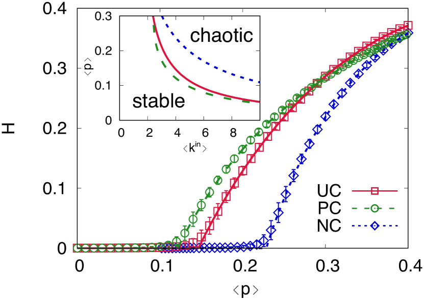
We implemented numerical simulations on ER networks with $\langle k^{in}\rangle=\langle k^{out}\rangle=4$ without any degree-degree correlation. We assigned the biases and corresponding Boolean variables according to the process described above. From initial states selected randomly, the state of each node are updated synchronously according to the Boolean variables. After a transient period, the trajectory will fall into a point or cycle attractor since the dynamics are deterministic. To simulate a perturbation, we flipped a fraction of $0.01$ of the nodes by force. When the system reached a point or cycle attractor again following the perturbation, we measured the Hamming distance over all nodes.

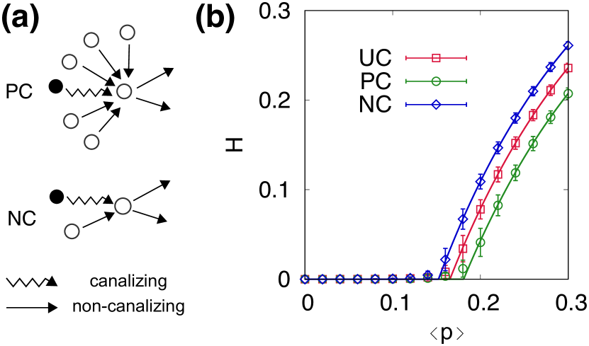
In Fig. 1, we compare the analytical predictions from Eq. 9 to the numerical simulations. The agreement between the theory and the simulations is excellent. We find that a negatively correlated sensitivity to degree enhances stability when comparing the UC and PC cases. For the NC case, the transition point of mean bias $\langle p\rangle_{c}$ is delayed and $H$ is lower than in the other cases. In contrast, the PC case exhibits an enlarged chaotic region compared to the other cases, making it more vulnerable to perturbations. These results demonstrate that the correlation between sensitivity and degree can significantly affect the stability in terms of the location of the critical point and the size of Hamming distance.

In order to examine the effect of the correlation in more realistic circuits, we consider two examples beyond ER networks: i) an empirical regulatory network conroy and ii) a network with a heavy-tailed out-degree distribution. First, we consider a real-world regulatory network of CD4⁺ T-cell with $N=188$ and $\langle k\rangle=3.73$ conroy . Each node and link in the network respectively represents proteins and protein-protein interactions. We assume every link in the network is bi-directional. We choose the CD4⁺ T-cell network as a representative example because the network is the second largest example in the all tested networks in the survey of empirical Boolean networks daniels2018 and also has a sufficient link density to examine the stability of the network. Second, we study networks with scale-free out-degrees and Poisson distributed in-degrees. The rationale behind these networks is that real transcriptional regulatory networks commonly possess a heavy-tailed out-degree distribution and a short-tailed in-degree distribution guelzim ; dobrin . We constructed $10^{3}$ different network realizations with size $N=10^{4}$ having scale-free out-degrees with the degree exponent $\gamma=2.5$ and Poisson distributed in-degrees with $\langle k_{in}\rangle=4.72\ldots$, according to the configuration model. We implemented numerical simulations on the two networks with three couplings as described above.

Figure 2: (a) Average Hamming distances $H$ of a real-world Boolean network for a CD4⁺ T-cell with $N=188$ and $\langle k\rangle=3.73$. (b) Average Hamming distances $H$ of Boolean networks with a scale-free out-degree distribution with the degree exponent $\gamma=2.5$ and a Poisson in-degree distribution with $\langle k_{in}\rangle\approx 4.72$. We generate $10^{3}$ different network realizations with $N=10^{4}$. We consider three types of correlated coupling (UC, PC, and NC). Analytical predictions (lines) and numerical results (symbols) are presented together.

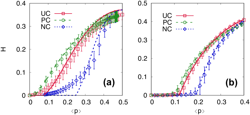
In Fig. 2, we show the analytical predictions and the numerical simulations (symbols) for the CD4⁺ T-cell network and scale-free out-degree distribution network. The theory (lines) based on Eqs. 2 and 3 shows well agreement with the simulations in a qualitative manner. Deviation from the theory in the CD4⁺ network shown in Fig. 2(a) is due to the short loops and small size of the real network. We find again a negatively correlated sensitivity to degree increases the stability of Boolean dynamics when comparing the UC and PC cases. We confirm the delayed transition $\langle p\rangle_{c}$ to chaotic phase and lower $H$ for the NC coupling than the other cases. On the other hand, the PC coupling shows less stable behaviors to perturbations. There is an inversion between $H$ for UC and PC cases for $\langle p\rangle\gtrsim 0.25$, far above $\langle p\rangle_{c}$ in Fig. 2(b). In this region, low degree nodes with low bias in PC coupling suppress $H$, so that $H$ for PC is above that for UC. The similar crossing behaviors are often observed when one considers degree correlations such as assortative mixing assortative and interlayer degree correlations interlayer .

Figure 3: (a) Average Hamming distances of random Boolean networks with three types of correlated coupling and a bimodal in-degree distribution with $P(k^{in})=(1/2)\delta_{k^{in},10}+(1/2)\delta_{k^{in},6}$ and $N=10^{4}$. The bias distribution is also bimodal and defined as $Q(p)=(1/2)\delta_{p,2\langle p\rangle-1/2}+(1/2)\delta_{p,0.1}$. Analytical predictions (lines) and numerical results (symbols) are presented together. (b) Phase diagram between stable and chaotic phases obtained theoretically as a function of the mean node in-degree $\langle k^{in}\rangle$ and $p$. We use $K_{1}=\langle k^{in}\rangle+2$ and $K_{2}=\langle k^{in}\rangle-2$.

Figure 4: Comparison of the stability of each node obtained theoretically $H_{i}^{th}$ and through numerical simulations $H_{i}^{sim}$ with different types of coupling: (a) PC, (b) UC, and (c) NC. We consider a network with $P(k^{in})=(1/2)\delta_{k^{in},10}+(1/2)\delta_{k^{in},6}$ and $N=10^{4}$, and a bimodal bias distribution defined as $Q(p)=(1/2)\delta_{p,2\langle p\rangle-1/2}+(1/2)\delta_{p,0.1}$. Note the changed axes for (c). The average Hamming distances for nodes with high in-degree ($k^{in}=10$) and low degree ($k^{in}=6$) are denoted by red and blue arrows, respectively. The average Hamming distance over all nodes is denoted by a filled circle.

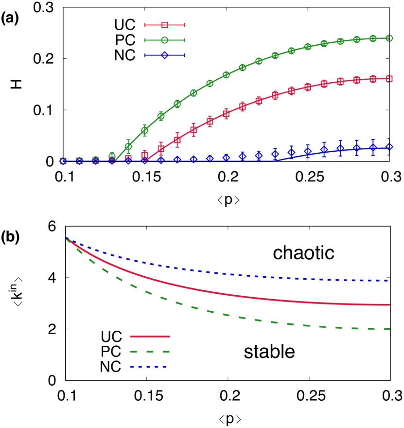
To evaluate the impact of the interplay between node degree and sensitivity more clearly, we consider a transparent example with a bimodal in-degree distribution $P(k^{in})=(1/2)\delta_{k^{in},K_{1}}+(1/2)\delta_{k^{in},K_{2}}$, where $\delta_{i,j}$ represents the Kronecker delta. We construct networks with the bimodal in-degree and Poisson distributed out-degree distribution according to the configuration model. We assign a bias drawn from a bimodal distribution $Q(p)=(1/2)\delta_{p,\phi_{1}}+(1/2)\delta_{p,\phi_{2}}$. Similar to the analysis above, we consider three types of correlated coupling: UC, PC, and NC. For the UC case, we assign a bias to each node at random, independent of the node degree. Positively (negatively) correlated coupling can be achieved by ensuring that higher (lower) degree nodes have greater bias values. In our examples, we use $K_{1}=10$, $K_{2}=6$, $\phi_{1}=2\langle p\rangle-1/2$, and $\phi_{2}=0.1$, where $0.1\leq\phi_{1}\leq 0.5$. Note that the range of $\langle p\rangle$ is $0.1\leq\langle p\rangle\leq 0.3$. By annealing the probability $H_{i}$, we can derive the self-consistency equation for $H_{a}$ as follows:

$$\text{UC:}\ H_{a} =\frac{1}{2}\left(q_{1}+q_{2}\right)\left[2-(1-H_{a})^{K_{1}}-(1-H_{a})^{K_{2}}\right],$$

$$\text{PC:}\ H_{a} =\frac{1}{2}q_{1}\left[1-(1-{H_{a}})^{K_{1}}\right]+\frac{1}{2}q_{2}\left[1-(1-{H_{a}})^{K_{2}}\right],$$

$$\text{NC:}\ H_{a} =\frac{1}{2}q_{2}\left[1-(1-{H_{a}})^{K_{1}}\right]+\frac{1}{2}q_{1}\left[1-(1-{H_{a}})^{K_{2}}\right],$$ (10)

where $q_{1}=2\phi_{1}(1-\phi_{1})$ and $q_{2}=2\phi_{2}(1-\phi_{2})$.

As shown in Fig. 3, negatively correlated coupling is more resilient to external perturbations compared to the other types of coupling. The average Hamming distance clearly highlights the effect of the correlation between sensitivity and local node in-degree. Specifically, negative correlation between sensitivity and node degree enhances the global stability of Boolean networks [Fig. 3(a)]. For the NC case, the majority of incoming links are connected to unbiased nodes ($p=1/2$), leading to more stable Boolean dynamics. In contrast, for the PC case, damage can easily spread through an entire network because an adequate fraction of high-degree nodes have high sensitivity. Fig. 3(b) presents a phase diagram as functions of the mean node degree $\langle k^{in}\rangle$ and $\langle p\rangle$, where $K_{1}=\langle k^{in}\rangle+2$ and $K_{2}=\langle k^{in}\rangle-2$. An increasing value of $p_{c}$ for the NC coupling can be observed consistently over a wide range of parameter sets.

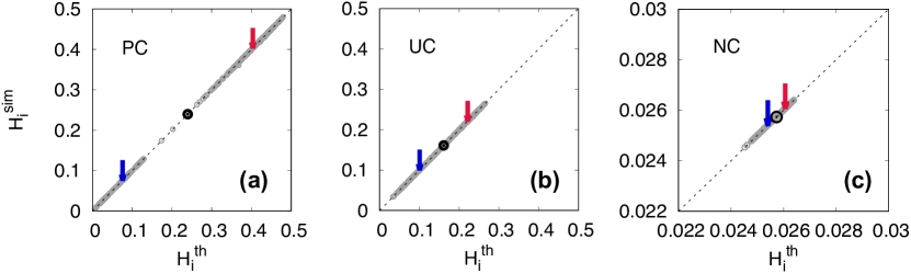
In addition to the global stability of Boolean networks, we can also assess the stability of each node in a given network topology using Eq. 2. Fig. 4 reveals perfect agreement between the numerical results $H_{i}^{sim}$ and theoretical predictions $H_{i}^{th}$ for the probability that a node $i$ changes its state when a perturbation occurs. We computed the average Hamming distances $\langle H(k^{in}=10)\rangle$ and $\langle H(k^{in}=6)\rangle$ for nodes with high in-degree ($k^{in}=10$) and low in-degree ($k^{in}=6$), respectively, as indicated by the red and blue arrows in Fig. 4, respectively. The average Hamming distance over all nodes is denoted by a filled circle. One can see two clearly separated groups of nodes with different stability values and Hamming distances $H_{i}$ for the PC coupling. We can confirm that in the PC coupling, damage can spread through high in-degree nodes with high sensitivity, which are prone to instability. However, for the NC coupling, these two groups merge and perturbations terminate quickly. From the perspective of a percolation problem, NC coupling corresponds to the case where high in-degree nodes have low occupation probabilities, leading to stable dynamics, which is analogous to degree-based removal in network percolation attack .

Finally, we consider the role of the interplay between local node in-degree and canalizing inputs moreira2005 ; daniels2018 . Canalizing functions have a single input that forces the corresponding output to a specific value, regardless of the values of other inputs. The Hamming distance $H_{i}$ for each node $i$ with a fraction $c_{i}$ of canalizing inputs is calculated as squires2012

$$H_{i}= c_{i}q_{i}H_{ic}+\frac{1}{2}c_{i}q_{i}(1-H_{ic})\left[1-\prod_{j\in\partial i/c}(1-H_{j})\right]$$

$$\quad+(1-c_{i})q_{i}\left[1-\prod_{j\in\partial i}(1-H_{j})\right],$$ (11)

where $H_{ic}$ is the Hamming distance of the neighbor of node $i$ connected by a canalizing input, $q_{j}=2p_{j}(1-p_{j})$, $\partial j/c$ define a set of inputs excluding a canalizing input squires2012 . By definition, canalizing functions lead to stable dynamics moreira2005 because they effectively reduce the sensitivity of non-canalizing inputs connected to nodes shared by canalizing inputs. However, the effects of canalizing inputs are not solely determined by the fraction of canalizing inputs. The topological locations of canalizing links also affect stability, which can be predicted using Eq. 11.

We consider three different correlations between node in-degree and the locations of canalizing inputs, which are again denoted as UC, PC, and NC. For the UC case, the canalizing inputs are distributed randomly. For the PC (NC) case nodes with high (low) in-degree tend to have a canalizing input. For the sake of simplicity, we consider a random network with a bimodal in-degree distribution defined as $P(k^{in})=(1/2)\delta_{k^{in},K_{1}}+(1/2)\delta_{k^{in},K_{2}}$, where $K_{1}=6$ and $K_{2}=2$. In this example, we assume that $1/4$ of the nodes have a canalizing input and each node can have at most one canalizing input. For the UC case, a quarter of nodes chosen at random have a canalizing input. For the PC case, the low in-degree nodes ($k^{in}=2$) do not have a canalizing input and a half of high in-degree nodes ($k^{in}=6$) have a canalizing input. On the other hand, for the NC case only low in-degree nodes have a canalizing input with the probability $1/2$ [see Fig. 5(a)].

As shown in Fig. 5(b), correlation between canalizing inputs and local node in-degree can increase global stability. Specifically, the PC coupling enhances the stability of Boolean networks. In contrast, the NC coupling decreases stability, leading to smaller $p_{c}$ and larger $H$ values. In this example, one can see that correlation between local node degree and canalizing inputs alters Boolean dynamics significantly. When a canalizing input becomes active, all other connections are ineffective. Therefore, for the PC case, a larger fraction of non-canalizing inputs lose their influence on Boolean dynamics to the canalizing inputs. In the NC case, the effects of canalizing inputs are minimized because they only affect low in-degree nodes.

Figure 5: (a) Diagram of coupling between node degree and canalizing inputs. For the PC and NC cases, nodes with high and low in-degree respectively tend to have a canalizing input. (b) Average Hamming distance with canalizing inputs as a function of $\langle p\rangle$ with the UC, PC, and NC cases.

IV Discussion

We analyzed the stability of random Boolean networks incorporating dynamic rules, as well as the topological properties of each node. We find that correlation between node degree and Boolean functions plays an important role in determining Hamming distances and critical point. Specifically, negatively correlated sensitivity to the in-degree of each node increases stability. We also find that a correlation between high-degree nodes and canalizing inputs can increase global stability. Our results reveal that analysis based on the naive mean-field approach may fail to predict dynamical consequences in Boolean networks with intertwined structural and functional properties, which are often observed in real-world biological systems. Further study is required to examine the effects of more complex features in Boolean networks, such as loops and feedback in network topologies kinoshita ; cho , and hierarchical dynamics.

Data Availability

The data that supports the findings of this study are available within the article.

References

- (1) S. A. Kauffman, J. Theoret. Biol. 22, 437 (1969).
- (2) G. Karlebach and R. Shamir, Nat. Rev. Mol. Cell Biol. 9, 770 (2008).
- (3) I. Albert, J. Thakar, S. Li, R. Zhang, and R. Albert, Source Code Biol. Med. 3, 16 (2008).
- (4) F. Li, T. Long, Y. Lu, Q. Ouyang, and C. Tang, Proc. Natl. Acad. Sci. 101, 4781 (2004).
- (5) R. Thomas and M. Kaufman, Chaos 11, 180-195 (2001).
- (6) I. Shmulevich, E. R. Dougherty, and W. Zhang, Bioinformatics 18, 1319 (2002).
- (7) D. P. Rosin, D. Rontani, D. J. Gauthier, and E. Schöll, Phys. Rev. Lett. 110, 104102 (2013).
- (8) H. Sayama, I. Pestov, J. Schmidt, B. J. Bush, C. Wong, J. Yamanoi, and T. Gross, Comput. Math. Appl. 65, 1645 (2013).
- (9) S. A. Kauffman, The origins of order: self-organization and selection in evolution, (Oxford University Press, New York, 1993).
- (10) M. A. Mũnoz, Rev. Mod. Phys. 90, 031001 (2018).
- (11) D. Krotov, J. O. Dubuis, T. gregor, and W. Bialek, Proc. Natl. Acad. Sci. 111, 3683 (2014).
- (12) B. C. Daniels, H. Kim, D. Moore, S. Zhou, H. B. Smith, B. Karas, S. A. Kauffman, and S. I. Walker, Phys. Rev. Lett. 121, 138102 (2018).
- (13) R. Serra, M. Villani, and A. Semeria, J. Theor. Biol. 227, 149 (2004).
- (14) M. Nykter, N. D. Price, M. Aldana, S. A. Ramsey, S. A. Kauffman, L. E. Hood, O. Yli-Harja, and I. Shmulevich, Proc. Natl. Acad. Sci. 105, 1897 (2008).
- (15) B. Derrida and Y. Pomeau, EPL (Europhys. Lett.) 1, 45 (1986).
- (16) B. Luque and R. V. Sole, Phys. Rev. E 55, 257 (1997).
- (17) M. Aldana and P. Cluzel, Proc. Natl. Acad. Sci. 100, 8710 (2003).
- (18) D.-S. Lee and H. Rieger, J. Phys. A: Math. Theor. 41, 415001 (2008).
- (19) T. P. Peixoto and B. Drossel, Phys. Rev. E 79, 036108 (2009).
- (20) P. Villegas, J. Ruiz-Franco, J. Hidalgo, and M. A. Muñoz, Sci. Rep. 6, 34743 (2016).
- (21) E. Cozzo, A. Arenas, and Y. Moreno, Phys. Rev. E 86, 036115 (2012).
- (22) K. Klemm and S. Bornholdt, Phys. Rev. E 72, 055101(R) (2005).
- (23) F. Ghanbarnejad and K. Klemm, Phys. Rev. Lett. 107, 188701 (2011).
- (24) H. Ebadi and K. Klemm, Phys. Rev. E 90, 022815 (2014).
- (25) D. Lee, K.-I. Goh, and B. Kahng, Phys. Rev. E 86, 027101 (2012).
- (26) G. Boldhaus, N. Bertschinger, J. Rauh, E. Olbrich, and K. Klemm, Phys. Rev. E 82, 021916 (2010).
- (27) J. Wang, S. Pei, W. Wei, X. Feng, and Z. Zheng, Phys. Rev. E 97, 032305 (2018).
- (28) A. Goudarzi, C. Teuscher, N. Gulbahce, and T. Rohlf, Phys. Rev. Lett. 108, 128702 (2012).
- (29) A. A. Moreira and L. A. N. Amaral, Phys. Rev. Lett. 94, 218702 (2005).
- (30) I. Shmulevich and S. A. Kauffman, Phys. Rev. Lett. 93(4), 048701 (2004).
- (31) S. Squires, A. Pomerance, M. Girvan, and E. Ott, Phys. Rev. E 90, 022814 (2014).
- (32) A. Pomerance, E. Ott, M. Girvan, and W. Losert, Proc. Natl. Acad. Sci. 106, 8209 (2009).
- (33) S. Squires, E. Ott, and M. Girvan, Phys. Rev. Lett. 108, 085701 (2012).
- (34) B. Min, Eur. Phys. J. B 91, 18 (2018).
- (35) B. Min and C. Castellano, Chaos 30, 023131 (2020).
- (36) B. D. Conroy, et. al., Front. Immunol. 5, 599 (2014).
- (37) N. Guelzim, S. Bottani, P. Bourgine, and F. Kepes, Nat. Genet. 31, 60 (2002).
- (38) R. Dobrin, Q. K. Beg, A.-L. Barabási, and Z. N. Oltvai, BMC Bioinformatics 5, 10 (2004).
- (39) M. E. J. Newman, Phys. Rev. Lett. 89, 208701 (2002).
- (40) B. Min, S. D. Yi, K.-M. Lee, and K.-I. Goh, Phys. Rev. E 89, 042811 (2014).
- (41) R. Albert, H. Jeong, and A.-L. Barabási, Nature 406, 378-382 (2000).
- (42) S. Kinoshita and H. S. Yamada, Open Journal of Biophysics 9, 10-20 (2019).
- (43) Y.-K. Kwon and K.-H. Cho, BMC Bioinformatics 8, 430 (2007).