Abstract

Estimation of the number of components (or order) of a finite mixture model is a long standing and challenging problem in statistics. We propose the Group-Sort-Fuse (GSF) procedure—a new penalized likelihood approach for simultaneous estimation of the order and mixing measure in multidimensional finite mixture models. Unlike methods which fit and compare mixtures with varying orders using criteria involving model complexity, our approach directly penalizes a continuous function of the model parameters. More specifically, given a conservative upper bound on the order, the GSF groups and sorts mixture component parameters to fuse those which are redundant. For a wide range of finite mixture models, we show that the GSF is consistent in estimating the true mixture order and achieves the $n^{-1/2}$ convergence rate for parameter estimation up to polylogarithmic factors. The GSF is implemented for several univariate and multivariate mixture models in the R package GroupSortFuse. Its finite sample performance is supported by a thorough simulation study, and its application is illustrated on two real data examples.

1 Introduction

Mixture models are a flexible tool for modelling data from a population consisting of multiple hidden homogeneous subpopulations. Applications in economics (Bosch-Domènech et al.,, 2010), machine learning (Goodfellow et al.,, 2016), genetics (Bechtel et al.,, 1993) and other life sciences (Thompson et al.,, 1998; Morris et al.,, 1996) frequently employ mixture distributions. A comprehensive review of statistical inference and applications of finite mixture models can be found in the book by McLachlan and Peel, (2000).

Given integers $N,d\geq 1$, let ${\cal F}=\{f(\mathbf{y};\bm{\theta}):\bm{\theta}=(\theta_{1},\ldots,\theta_{d})^{\top}\in\Theta\subseteq\mathbb{R}^{d},\ \mathbf{y}\in\mathcal{Y}\subseteq\mathbb{R}^{N}\}$ be a parametric family of density functions with respect to a $\sigma$-finite measure $\nu$, with a compact parameter space $\Theta$. The density function of a finite mixture model with respect to $\mathcal{F}$ is given by

$$p_{G}(\mathbf{y})=\int_{\Theta}f(\mathbf{y};\bm{\theta})\text{d}G(\bm{\theta})=\sum_{j=1}^{K}\pi_{j}f(\mathbf{y};\bm{\theta}_{j}),$$ (1.1)

where

$$G=\sum_{j=1}^{K}\pi_{j}\delta_{\bm{\theta}_{j}}$$ (1.2)

is the mixing measure with $\bm{\theta}_{j}=(\theta_{j1},\dots,\theta_{jd})^{\top}\in\Theta$, $j=1,\dots,K$, and the mixing probabilities $0\leq\pi_{j}\leq 1$ satisfy $\sum_{j=1}^{K}\pi_{j}=1$. Here, $\delta_{\bm{\theta}}$ denotes a Dirac measure placing mass at $\bm{\theta}\in\Theta$. The $\bm{\theta}_{j}$ are said to be atoms of $G$, and $K$ is called the order of the model.

Let $\mathbf{Y}_{1},\dots,\mathbf{Y}_{n}$ be a random sample from a finite mixture model (1.1) with true mixing measure $G_{0}=\sum_{j=1}^{K_{0}}\pi_{0j}\delta_{\bm{\theta}_{0j}}$. The true order $K_{0}$ is defined as the smallest number of atoms of $G_{0}$ for which the component densities $f(\cdot;\bm{\theta}_{0j})$ are different, and the mixing proportions $\pi_{0j}$ are non-zero. This paper is concerned with parametric estimation of $K_{0}$.

In practice, the order of a finite mixture model may not be known. An assessment of the order is important even if it is not the main object of study. Indeed, a mixture model whose order is less than the true number of underlying subpopulations provides a poor fit, while a model with too large of an order, which is said to be overfitted, may be overly complex and hence uninformative. From a theoretical standpoint, estimation of overfitted finite mixture models leads to a deterioration in rates of convergence of standard parametric estimators. Indeed, given a consistent estimator $G_{n}$ of $G_{0}$ with $K>K_{0}$ atoms, the parametric $n^{-1/2}$ convergence rate is generally not achievable. Under the so-called second-order strong identifiability condition, Chen, (1995) and Ho et al., 2016b showed that the optimal pointwise rate of convergence in estimating $G_{0}$ is bounded below by $n^{-1/4}$ with respect to an appropriate Wasserstein metric. In particular, this rate is achieved by the maximum likelihood estimator up to a polylogarithmic factor. Minimax rates of convergence have also been established by Heinrich and Kahn, (2018), under stronger regularity conditions on the parametric family $\mathcal{F}$. Remarkably, these rates deteriorate as the upper bound $K$ increases. This behaviour has also been noticed for pointwise estimation rates in mixtures which do not satisfy the second-order strong identifiability assumption—see for instance Chen and Chen, (2003) and Ho et al., 2016a . These results warn against fitting finite mixture models with an incorrectly specified order. In addition to poor convergence rates, the consistency of $G_{n}$ does not guarantee the consistent estimation of the mixing probabilities and atoms of the true mixing measure, though they are of greater interest in most applications.

The aforementioned challenges have resulted in the development of many methods for estimating the order of a finite mixture model. It is difficult to provide a comprehensive list of the research on this problem, and thus we give a selective overview. One class of methods involves hypothesis testing on the order using likelihood-based procedures (McLachlan,, 1987; Dacunha-Castelle et al.,, 1999; Liu and Shao,, 2003), and the EM-test (Chen and Li,, 2009; Li and Chen,, 2010). These tests typically assume knowledge of a candidate order; when such a candidate is unavailable, estimation methods can be employed. Minimum distance-based methods for estimating $K_{0}$ have been considered by Chen and Kalbfleisch, (1996), James et al., (2001), Woo and Sriram, (2006), Heinrich and Kahn, (2018), and Ho et al., (2017). The most common parametric methods involve the use of an information criterion, whereby a penalized likelihood function is evaluated for a sequence of candidate models. Examples include Akaike’s Information Criterion (AIC; Akaike, (1974)) and the Bayesian Information Criterion (BIC; Schwarz, (1978)). The latter is arguably the most frequently used method for mixture order estimation (Leroux,, 1992; Keribin,, 2000; McLachlan and Peel,, 2000), though it was not originally developed for non-regular models. This led to the development of information criteria such as the Integrated Completed Likelihood (ICL; Biernacki et al., (2000)), and the Singular BIC (sBIC; Drton and Plummer, (2017)). Bayesian approaches include the method of Mixtures of Finite Mixtures, whereby a prior is placed on the number of components (Nobile,, 1994; Richardson and Green,, 1997; Stephens,, 2000; Miller and Harrison,, 2018), and model selection procedures based on Dirichlet Process mixtures, such as those of Ishwaran et al., (2001) and the Merge-Truncate-Merge method of Guha et al., (2019). Motivated by regularization techniques in regression, Chen and Khalili, (2008) proposed a penalized likelihood method for order estimation in finite mixture models with a one-dimensional parameter space $\Theta$, where the regularization is applied to the difference between sorted atoms of the overfitted mixture model. Hung et al., (2013) adapted this method to estimation of the number of states in Gaussian Hidden Markov models, which was also limited to one-dimensional parameters for different states. Despite its model selection consistency and good finite sample performance, the extension of this method to multidimensional mixtures has not been addressed. In this paper, we take on this task and propose a far-reaching generalization called the Group-Sort-Fuse (GSF) procedure.

The GSF postulates an overfitted finite mixture model with a large tentative order $K>K_{0}$. The true order $K_{0}$ and the mixing measure $G_{0}$ are simultaneously estimated by merging redundant mixture components, by applying two penalties to the log-likelihood function of the model. The first of these penalties groups the estimated atoms, while the second penalty shrinks the distances between those which are in high proximity. The latter is achieved by applying a sparsity-inducing regularization function to consecutive distances between these atoms, sorted using a so-called cluster ordering (Definition 2). Unlike most existing methods, this form of regularization, which uses continuous functions of the model parameters as penalties, circumvents the fitting of mixture models of all orders $1,2,\dots,K$. In our simulations we noticed that using EM-type algorithms (Dempster et al.,, 1977), the GSF is less sensitive to the choice of starting values than methods which involve maximizing likelihoods of mixture models with different orders. By increasing the amount of regularization, the GSF produces a series of fitted mixture models with decreasing orders, as shown in Figure 1 for a simulated dataset. This qualitative representation, inspired by coefficient plots in penalized regression (Friedman et al.,, 2008), can also provide insight on the mixture order and parameter estimates for purposes of exploratory data analysis.

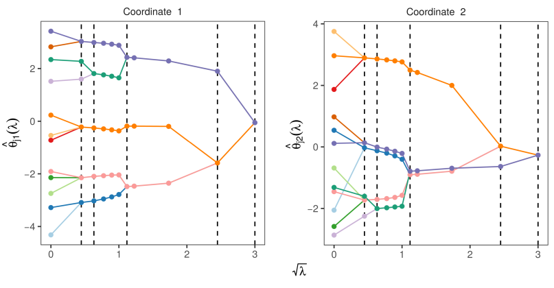
Figure 1: Regularization plots based on simulated data from a location-Gaussian mixture with $K_{0}=5,d=2$. The fitted atoms $\widehat{\bm{\theta}}_{j}(\lambda)=(\widehat{\theta}_{j1}(\lambda),\widehat{\theta}_{j2}(\lambda))^{\top}$, $j=1,\dots,K=12$, are plotted against a regularization parameter $\lambda$. Across coordinates, each estimated atom is identified by a unique color.

The main contributions of this paper are summarized as follows. For a wide range of second-order strongly identifiable parametric families, the GSF is shown to consistently estimate the true order $K_{0}$, and achieves the $n^{-1/2}$ rate of convergence in parameter estimation up to polylogarithmic factors. To achieve this result, the sparsity-inducing penalties used in the GSF must satisfy conditions which are nonstandard in the regularization literature. We also derived, for the first time, sufficient conditions for the strong identifiability of multinomial mixture models. Thorough simulation studies based on multivariate location-Gaussian and multinomial mixture models show that the GSF performs well in practice. The method is implemented for several univariate and multivariate mixture models in the R package GroupSortFuse.

The rest of this paper is organized as follows. We describe the GSF method, and compare it to a naive alternative in Section 2. Asymptotic properties of the method are studied in Section 3. Our simulation results and two real data examples are respectively presented in Sections 4 and 5, and Supplement E.6. We close with some discussions in Section 6. Proofs, numerical implementation, and additional simulation results are given in Supplements A–F.

Notation. Throughout the paper, $|A|$ denotes the cardinality of a set $A$, and for any integer $K\geq 1$, $A^{K}=A\times...\times A$ denotes the $K$-fold Cartesian product of $A$ with itself. $S_{K}$ denotes the set of permutations on $K$ elements $\{1,2,\ldots,K\}$. Given a vector $\mathbf{x}=(x_{1},\dots,x_{d})^{\top}\in\mathbb{R}^{d}$, we denote its $\ell_{p}$-norm by $\left\lVert\mathbf{x}\right\rVert_{p}=\left(\sum_{j=1}^{d}|x_{j}|^{p}\right)^{1/p}$, for all $1\leq p<\infty$. In the case of the Euclidean norm $\left\lVert\cdot\right\rVert_{2}$, we omit the subscript and write $\left\lVert\cdot\right\rVert$. The diameter of a set $A\subseteq\mathbb{R}^{d}$ is denoted $\text{diam}(A)=\sup\{\|x-y\|:x,y\in A\}$. Given two sequences of real numbers $\{a_{n}\}_{n=1}^{\infty}$ and $\{b_{n}\}_{n=1}^{\infty}$, we write $a_{n}\lesssim b_{n}$ to indicate that there exists a constant $C>0$ such that $a_{n}\leq Cb_{n}$ for all $n\geq 1$. We write $a_{n}\asymp b_{n}$ if $a_{n}\lesssim b_{n}\lesssim a_{n}$. For any $a,b\in\mathbb{R}$, we write $a\wedge b=\min\{a,b\}$, $a\vee b=\max\{a,b\}$, and $a_{+}=a\vee 0$. Finally, we let ${\cal G}_{K}=\{G:G=\sum_{j=1}^{K}\pi_{j}\delta_{\bm{\theta}_{j}},\leavevmode\nobreak\ \bm{\theta}_{j}\in\Theta,\pi_{j}\geq 0,\sum_{j=1}^{K}\pi_{j}=1\}$ be the class of mixing measures with at most $K$ components.

Figures. All the numerical and algorithmic details of the illustrative figures throughout this paper are given in Section 4 and Supplement D.

2 The Group-Sort-Fuse (GSF) Method

Let $\mathbf{Y}_{1},\dots,\mathbf{Y}_{n}$ be a random sample arising from $p_{G_{0}}$, where $G_{0}\in\mathcal{G}_{K_{0}}$ is the true mixing measure with unknown order $K_{0}$. Assume an upper bound $K$ on $K_{0}$ is known—further discussion on the choice of $K$ is given in Section 3.3. The log-likelihood function of a mixing measure $G$ with $K>K_{0}$ atoms is said to be overfitted, and is defined by

$$l_{n}(G)=\sum_{i=1}^{n}\log p_{G}(\mathbf{Y}_{i}).$$ (2.1)

The overfitted maximum likelihood estimator (MLE) of $G$ is given by

$$\bar{G}_{n}=\sum_{j=1}^{K}\bar{\pi}_{j}\delta_{\bar{\bm{\theta}}_{j}}=\operatorname*{argmax}_{G\in\mathcal{G}_{K}}l_{n}(G).$$ (2.2)

As discussed in the Introduction, though the overfitted MLE is consistent in estimating $G_{0}$ under suitable metrics, it suffers from slow rates of convergence, and there may exist atoms of $\bar{G}_{n}$ whose corresponding mixing probabilities vanish, and do not converge to any atoms of $G_{0}$. Furthermore, from a model selection standpoint, $\bar{G}_{n}$ typically has order greater than $K_{0}$. In practice, $\bar{G}_{n}$ therefore overfits the data in the following two ways which we will refer to below: (a) certain fitted mixing probabilities $\bar{\pi}_{j}$ may be near-zero, and (b) some of the estimated atoms $\bar{}\bm{\theta}_{j}$ may be in high proximity to each other. In this section, we propose a penalized maximum likelihood approach which circumvents both types of overfitting, thus leading to a consistent estimator of $K_{0}$.

Overfitting (a) can readily be addressed by imposing a lower bound on the mixing probabilities, as was considered by Hathaway, (1986). This lower bound, however, could be particularly challenging to specify in overfitted mixture models. An alternative approach is to penalize against near-zero mixing probabilities (Chen and Kalbfleisch,, 1996). Thus, we begin by considering the following preliminary penalized log-likelihood function

$$l_{n}(G)-\varphi(\pi_{1},\dots,\pi_{K}),\quad\ G\in\mathcal{G}_{K},$$ (2.3)

where $\varphi\equiv\varphi_{n}$ is a nonnegative penalty function such that $\inf_{n\geq 1}\varphi_{n}(\pi_{1},\dots,\pi_{K})\to\infty$ as $\min_{1\leq j\leq K}\pi_{j}$ $\to 0$. We further require that $\varphi$ is invariant to relabeling of its arguments, i.e. $\varphi(\pi_{1},\dots,\pi_{K})=\varphi(\pi_{\tau(1)},\dots,\pi_{\tau(K)})$, for any permutation $\tau\in S_{K}$. Examples of $\varphi$ are given at the end of this section. The presence of this penalty ensures that the maximizer of (2.3) has mixing probabilities which stay bounded away from zero. Consequently, as shown in Theorem 1 below, this preliminary estimator is consistent in estimating the atoms of $G_{0}$, unlike the overfitted MLE in (2.2). It does not, however, consistently estimate the order $K_{0}$ of $G_{0}$, as it does not address overfitting (b).

Our approach is to introduce a second penalty which has the effect of merging fitted atoms that are in high proximity. We achieve this by applying a sparsity-inducing penalty $r_{\lambda_{n}}$ to the distances between appropriately chosen pairs of atoms of the overfitted mixture model with order $K$. It is worth noting that one could naively apply $r_{\lambda_{n}}$ to all ${K\choose 2}$ pairwise atom distances. Our simulations, however, suggest that such an exhaustive form of penalization increases the sensitivity of the estimator to the upper bound $K$, as shown in Figure 3. Instead, given a carefully chosen sorting of the atoms in $\mathbb{R}^{d}$, our method merely penalizes their $K-1$ consecutive distances. This results in the double penalized log-likelihood $L_{n}(G)$ in (2.6), which we now describe using the following definitions.

Definition 1.

Let $\mathbf{t}_{1},\dots,\mathbf{t}_{K}\in\Theta\subseteq\mathbb{R}^{d}$, and let $\mathcal{P}=\{\mathcal{C}_{1},\dots,\mathcal{C}_{H}\}$ be a partition of $\{\mathbf{t}_{1},\dots,\mathbf{t}_{K}\}$, for some integer $1\leq H\leq K$. Suppose

$$\max_{\mathbf{t}_{i},\mathbf{t}_{j}\in\mathcal{C}_{h}}\left\lVert\mathbf{t}_{i}-\mathbf{t}_{j}\right\rVert<\min_{\begin{subarray}{c}\mathbf{t}_{i}\in\mathcal{C}_{h}\\ \mathbf{t}_{l}\not\in\mathcal{C}_{h}\end{subarray}}\left\lVert\mathbf{t}_{i}-\mathbf{t}_{l}\right\rVert,\quad h=1,\dots,H.$$ (2.4)

Then, each set $\mathcal{C}_{h}$ is said to be an atom cluster, and $\mathcal{P}$ is said to be a cluster partition.

According to Definition 1, a partition is said to be a cluster partition if the within-cluster distances between atoms are always smaller than the between-cluster distances. The penalization in (2.3) (asymptotically) induces a cluster partition $\{\mathcal{C}_{1},\dots,\mathcal{C}_{K_{0}}\}$ of the estimated atoms. Heuristically, the estimated atoms falling within each atom cluster $\mathcal{C}_{h}$ approximate some true atom $\bm{\theta}_{0j}$, and the goal of the GSF is to merge these estimates, as illustrated in Figure 2. To do so, the GSF hinges on the notion of cluster ordering—a generalization of the natural ordering on the real line, which we now define.

Definition 2.

Let $\mathbf{t}=(\mathbf{t}_{1},\dots,\mathbf{t}_{K})\in\Theta^{K}$. A cluster ordering is a permutation $\alpha_{\mathbf{t}}\in S_{K}$ such that the following two properties hold.

1. Symmetry. For any permutation $\tau\in S_{K}$, if $\mathbf{t}^{\prime}=(\mathbf{t}_{\tau(1)},\dots,\mathbf{t}_{\tau(K)})$, then $\alpha_{\mathbf{t}^{\prime}}=\alpha_{\mathbf{t}}$.

2. Atom Ordering. For any integer $1\leq H\leq K$ and for any cluster partition $\mathcal{P}=\{\mathcal{C}_{1},\dots,\mathcal{C}_{H}\}$ of $\{\mathbf{t}_{1},\dots,\mathbf{t}_{K}\}$, $\alpha_{\mathbf{t}}^{-1}(\{j:\mathbf{t}_{j}\in\mathcal{C}_{h}\})$ is a set of consecutive integers for all $h=1,\dots,H$.

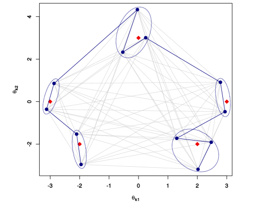
Figure 2: Illustration of a cluster partition $\mathcal{P}$ and a cluster ordering $\alpha_{\tilde{}\bm{\theta}}$ with $K=12$, based on the simulated sample used in Figure 1, with true atoms $\bm{\theta}_{01},\ldots,\bm{\theta}_{05}$ denoted by lozenges (◆), and atoms $\tilde{\bm{\theta}}=(\tilde{\bm{\theta}}_{1},\dots,\tilde{\bm{\theta}}_{12})$, obtained by maximizing the penalized log-likelihood (2.3), denoted by disks ($\bullet$). The ellipses ( …) represent a choice of $\mathcal{P}$ with $K_{0}=5$ atom clusters. The blue line (—) represents a cluster ordering $\alpha_{\tilde{\bm{\theta}}}$, in the sense that $\alpha_{\tilde{\bm{\theta}}}(1)$ is the index of the bottommost point, $\alpha_{\tilde{\bm{\theta}}}(2)$ is the index of the following point on the line, etc. The grey lines (—) represent all the pairwise distances penalized by the naive method defined in Figure 3.

If $t_{1},\dots,t_{K}\in\Theta\subseteq\mathbb{R}$ and $\mathbf{t}=(t_{1},\dots,t_{K})$, then the permutation $\alpha_{\mathbf{t}}\in S_{K}$ which induces the natural ordering $t_{\alpha_{\mathbf{t}}(1)}\leq\dots\leq t_{\alpha_{\mathbf{t}}(K)}$ is a cluster ordering. When $\Theta\subseteq\mathbb{R}^{d}$, property (ii) is satisfied for any permutation $\alpha_{\mathbf{t}}\in S_{K}$ such that

$$\alpha_{\mathbf{t}}(k)=\displaystyle\operatorname*{argmin}_{\begin{subarray}{c}1\leq j\leq K\\ j\not\in\{\alpha_{\mathbf{t}}(i):1\leq i\leq k-1\}\end{subarray}}\left\lVert\mathbf{t}_{j}-\mathbf{t}_{\alpha_{\mathbf{t}}(k-1)}\right\rVert,\quad k=2,\dots,K.$$ (2.5)

$\alpha_{\mathbf{t}}$ further satisfies property (i) provided $\alpha_{\mathbf{t}}(1)$ is invariant to relabeling of the components of $\mathbf{t}$. Any such choice of $\alpha_{\mathbf{t}}$ is therefore a cluster ordering in $\mathbb{R}^{d}$, and an example is shown in Figure 2 based on a simulated sample.

Given a mixing measure $G=\sum_{j=1}^{K}\pi_{j}\delta_{\bm{\theta}_{j}}$ with $\bm{\theta}=(\bm{\theta}_{1},\dots,\bm{\theta}_{K})$, let $\alpha_{\bm{\theta}}$ be a cluster ordering. For ease of notation, in what follows we write $\alpha\equiv\alpha_{\bm{\theta}}$. Let $\bm{\eta}_{j}=\bm{\theta}_{\alpha(j+1)}-\bm{\theta}_{\alpha(j)}$, for all $j=1,\dots,K-1$. We define the penalized log-likelihood function

$$L_{n}(G)=l_{n}(G)-\varphi(\pi_{1},\dots,\pi_{K})-n\sum_{j=1}^{K-1}r_{\lambda_{n}}(\left\lVert\bm{\eta}_{j}\right\rVert;\omega_{j}),$$ (2.6)

where the penalty $r_{\lambda_{n}}(\eta;\omega)$ is a non-smooth function at $\eta=0$ for all $\omega>0$, satisfying conditions (P1)–(P3) discussed in Section 3. In particular, $\lambda_{n}\geq 0$ is a regularization parameter, and $\omega_{j}\equiv\omega_{j}(G)>0$ are possibly random weights as defined in Section 3. Property (i) in Definition 2, and the invariance of $\varphi$ to relabelling of its arguments, guarantee that $L_{n}(G)$ is well-defined in the sense that it does not change upon relabelling the atoms of $G$. Finally, the Maximum Penalized Likelihood Estimator (MPLE) of $G$ is given by

$$\widehat{G}_{n}=\sum_{j=1}^{K}\widehat{\pi}_{j}\delta_{\widehat{\bm{\theta}}_{j}}=\operatorname*{argmax}_{G\in\mathcal{G}_{K}}L_{n}(G).$$ (2.7)

To summarize, the penalty $\varphi$ ensures the asymptotic existence of a cluster partition $\{\mathcal{C}_{1},\dots,\mathcal{C}_{K_{0}}\}$ of $\{\widehat{\bm{\theta}}_{1},\dots,\widehat{\bm{\theta}}_{K}\}$. Heuristically, the estimated atoms in each $\mathcal{C}_{h}$ approximate one of the atoms of $G_{0}$, and the goal of the GSF is to merge their values to be equal. To achieve this, Property (ii) of Definition 2 implies that any cluster ordering $\alpha$ is amongst the permutations in $S_{K}$ which maximize the number of indices $j$ such that $\bm{\theta}_{\alpha(j)},\bm{\theta}_{\alpha(j+1)}\in\mathcal{C}_{h}$, and minimize the number of indices $l$ such that $\bm{\theta}_{\alpha(l)}\in\mathcal{C}_{h}$ and $\bm{\theta}_{\alpha(l+1)}\not\in\mathcal{C}_{h}$, for all $h=1,\dots,K_{0}$. Thus our choice of $\alpha$ maximizes the number of penalty terms $r_{\lambda_{n}}(\left\lVert\bm{\eta}_{j}\right\rVert;\omega_{j})$ acting on distances between atoms of the same atom cluster $\mathcal{C}_{h}$. The non-differentiability of $r_{\lambda_{n}}$ at zero ensures that, asymptotically, $\widehat{\bm{\eta}}_{j}=\bm{0}$ or equivalently $\widehat{\bm{\theta}}_{\alpha(j)}=\widehat{\bm{\theta}}_{\alpha(j+1)}$ for certain indices $j$, and thus the effective order of $\widehat{G}_{n}$ becomes strictly less than the postulated upper bound $K$. This is how the GSF simultaneously estimates both the mixture order and the mixing measure. The choice of the tuning parameter $\lambda_{n}$ determines the size of the penalty $r_{\lambda_{n}}$ and thus the estimated mixture order. In Section 3, under certain regularity conditions, we prove the existence of a sequence $\lambda_{n}$ for which $\widehat{G}_{n}$ has order $K_{0}$ with probability tending to one, and in Section 4 we discuss data-driven choices of $\lambda_{n}$.

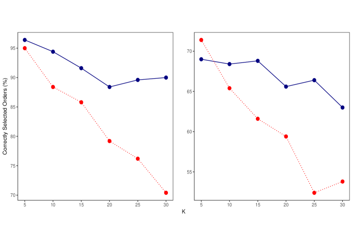
Figure 3: A comparison of the GSF (—), and the naive alternative ( …) given by $\operatorname*{argmax}_{G\in\mathcal{G}_{K}}\left\{l_{n}(G)-\varphi(\pi_{1},\dots,\pi_{K})-n\sum_{j\neq k}r_{\lambda_{n}}(\left\lVert\bm{\theta}_{j}-\bm{\theta}_{k}\right\rVert;\omega_{jk})\right\}$. The results are based on 500 simulated samples of size $n=200$ from the bivariate Gaussian mixture Models F.1 (left, $K_{0}=2$) and F.2 (right, $K_{0}=3$) given in Supplement F. Each point represents the percentage of times that a method with varying upper bounds $K$ correctly estimated $K_{0}$.

Examples of the penalties $\varphi$ and $r_{\lambda_{n}}$. We now discuss some examples of penalty functions $\varphi$ and $r_{\lambda_{n}}$. The functions $\varphi(\pi_{1},\dots,\pi_{K})\propto-\sum_{j=1}^{K}\log\pi_{j}$ and $\varphi(\pi_{1},\ldots,\pi_{K})\propto\sum_{j=1}^{K}\pi^{-\iota}_{j}$ (for some $\iota>0$) were used by Chen and Kalbfleisch, (1996) in the context of distance-based methods for mixture order estimation. As seen in Supplement D.1, the former is computationally convenient for EM-type algorithms, and we use it in all demonstrative examples throughout this paper. Li et al., (2009) also discuss the function $\varphi(\pi_{1},\ldots,\pi_{K})\propto-\min_{1\leq j\leq K}\log\pi_{j}$ in the context of hypothesis testing for the mixture order, which is more severe (up to a constant) than the former two penalties.

Regarding $r_{\lambda_{n}}$, satisfying conditions (P1)–(P3) in Section 3, we consider the following three penalties. For convenience, the first two penalties are written in terms of their first derivatives with respect to $\eta$.

1. The Smoothly Clipped Absolute Deviation (SCAD; Fan and Li, (2001)),

   $$r^{\prime}_{\lambda_{n}}(\eta;\omega)\equiv r^{\prime}_{\lambda_{n}}(\eta)=\lambda_{n}\leavevmode\nobreak\ I\{|\eta|\leq\lambda_{n}\}+\frac{(a\lambda_{n}-|\eta|)_{+}}{a-1}\leavevmode\nobreak\ I\{|\eta|>\lambda_{n}\},\qquad a>2.$$

2. The Minimax Concave Penalty (MCP; Zhang et al., 2010a ),

   $$r^{\prime}_{\lambda_{n}}(\eta;\omega)\equiv r^{\prime}_{\lambda_{n}}(\eta)=\left(\lambda_{n}-\frac{|\eta|}{a}\right)_{+},\qquad a>1.$$

3. The Adaptive Lasso (ALasso; Zou, (2006)),

   $$r_{\lambda_{n}}(\eta;\omega)=\lambda_{n}w|\eta|.$$

The Lasso penalty $r_{\lambda_{n}}(\eta;\omega)=\lambda_{n}|\eta|$ does not satisfy all the conditions (P1)–(P3), and is further discussed in Section 3.

3 Asymptotic Study

In this section, we study asymptotic properties of the GSF, beginning with preliminaries. We also introduce more notation in the sequence that it will be needed. Throughout this section, except where otherwise stated, we fix $K\geq K_{0}$.

3.1 Preliminaries

Inspired by Nguyen, (2013), we analyze the convergence of mixing measures in $\mathcal{G}_{K}$ using the Wasserstein distance. Recall that the Wasserstein distance of order $r\geq 1$ between two mixing measures $G=\sum_{j=1}^{K}\pi_{j}\delta_{\bm{\theta}_{j}}$ and $G^{\prime}=\sum_{k=1}^{K^{\prime}}\pi^{\prime}_{k}\delta_{\bm{\theta}_{k}^{\prime}}$ is given by

$$W_{r}(G,G^{\prime})=\left(\inf_{\mathbf{q}\in\mathcal{Q}(\bm{\pi},\bm{\pi}^{\prime})}\sum_{j=1}^{K}\sum_{k=1}^{K^{\prime}}q_{jk}\left\lVert\bm{\theta}_{j}-\bm{\theta}_{k}^{\prime}\right\rVert^{r}\right)^{\frac{1}{r}},$$ (3.1)

where $\mathcal{Q}(\bm{\pi},\bm{\pi}^{\prime})$ denotes the set of joint probability distributions $\mathbf{q}=\{q_{jk}:1\leq j\leq K,\ 1\leq k\leq K^{\prime}\}$ supported on $\{1,\dots,K\}\times\{1,\dots,K^{\prime}\}$, such that $\sum_{j=1}^{K}q_{jk}=\pi_{k}^{\prime}$ and $\sum_{k=1}^{K^{\prime}}q_{jk}=\pi_{j}$. We note that the $\ell_{2}$-norm of the underlying parameter space $\Theta$ is embedded into the definition of $W_{r}$. The distance between two mixing measures is thus largely controlled by that of their atoms. The definition of $W_{r}$ also bypasses the non-identifiability issues arising from mixture label switching. These considerations make the Wasserstein distance a natural metric for the space $\mathcal{G}_{K}$.

A condition which arises in likelihood-based asymptotic theory of finite mixture models with unknown order, called strong identifiability (in the second-order), is defined as follows.

Definition 3 (Strong Identifiability; Chen, (1995); Ho et al., 2016b ).

The family $\mathcal{F}$ is said to be strongly identifiable (in the second-order) if $f(\mathbf{y};\bm{\theta})$ is twice differentiable with respect to $\bm{\theta}$ for all $\mathbf{y}\in\mathcal{Y}$, and the following assumption holds for all integers $K\geq 1$.

1. Given distinct $\bm{\theta}_{1},\dots,\bm{\theta}_{K}\in\Theta$, if we have $\zeta_{j}\in\mathbb{R}$, $\bm{\beta}_{j},\bm{\gamma}_{j}\in\mathbb{R}^{d}$, $j=1,\ldots,K$, such that

   $$\operatorname*{ess\,sup}_{\mathbf{y}\in\mathcal{Y}}\left|\sum_{j=1}^{K}\left\{\zeta_{j}f(\mathbf{y};\bm{\theta}_{j})+\bm{\beta}_{j}^{\top}\frac{\partial f(\mathbf{y};\bm{\theta}_{j})}{\partial\bm{\theta}}+\bm{\gamma}_{j}^{\top}\frac{\partial^{2}f(\mathbf{y};\bm{\theta}_{j})}{\partial\bm{\theta}\partial\bm{\theta}^{\top}}\bm{\gamma}_{j}\right\}\right| =0$$

   then $\zeta_{j}=0$, $\bm{\beta}_{j}=\bm{\gamma}_{j}=\bm{0}\in\mathbb{R}^{d}$, for all $j=1,\dots,K$.

For strongly identifiable mixture models, the likelihood ratio statistic with respect to the overfitted MLE $\bar{G}_{n}$ is stochastically bounded (Dacunha-Castelle et al.,, 1999). In addition, under condition (SI), upper bounds relating the Wasserstein distance between a mixing measure $G$ and $G_{0}$ to the Hellinger distance between the corresponding densities $p_{G}$ and $p_{G_{0}}$ have been established by Ho et al., 2016b . In particular, there exist $\delta_{0},c_{0}>0$ depending on the true mixing measure $G_{0}$ such that for any $G\in\mathcal{G}_{K}$ satisfying $W_{2}(G,G_{0})<\delta_{0}$,

$$h(p_{G},p_{G_{0}})\geq c_{0}W_{2}^{2}(G,G_{0}),$$ (3.2)

where $h$ denotes the Hellinger distance,

$$h(p_{G},p_{G_{0}})=\left(\frac{1}{2}\int\big{(}\sqrt{p_{G}}-\sqrt{p_{G_{0}}}\big{)}^{2}d\nu\right)^{\frac{1}{2}}.$$

Specific statements and discussion of these results are given in Supplement B, and are used throughout the proofs of our Theorems 1-3. Further discussion of condition (SI) is given in Section 3.3. We also require regularity conditions (A1)–(A4) on the family $\mathcal{F}$, condition (C) on the cluster ordering $\alpha_{\mathbf{t}}$, and condition (F) on the penalty $\varphi$, which we state below.

Define the family of mixture densities

$$\mathcal{P}_{K}=\left\{p_{G}(\mathbf{y})=\int_{\bm{\Theta}}f(\mathbf{y};\bm{\theta})dG(\bm{\theta}):G\in\mathcal{G}_{K}\right\}.$$ (3.3)

Let $p_{0}=p_{G_{0}}$ be the density of the true finite mixture model with its corresponding probability distribution $P_{0}$. Furthermore, define the empirical process

$$\nu_{n}(G)=\sqrt{n}\int_{\{p_{0}>0\}}\frac{1}{2}\log\bigg{\{}\frac{p_{G}+p_{0}}{2p_{0}}\bigg{\}}d(P_{n}-P_{0}),\quad G\in\mathcal{G}_{K},$$ (3.4)

where $P_{n}=\frac{1}{n}\sum_{i=1}^{n}\delta_{\mathbf{Y}_{i}}$ denotes the empirical measure.

For any $\bm{\theta}=(\theta_{1},\dots,\theta_{d})^{\top}\in\Theta$, $\mathbf{y}\in\mathcal{Y}$, and $G\in\mathcal{G}_{K}$, let

$$U(\mathbf{y};\bm{\theta},G) = \frac{1}{p_{G}(\mathbf{y})}f(\mathbf{y};\bm{\theta})$$ (3.5)

$$U_{\kappa_{1}\ldots\kappa_{M}}(\mathbf{y};\bm{\theta},G) = \frac{1}{p_{G}(\mathbf{y})}\frac{\partial^{M}f(\mathbf{y};\bm{\theta})}{\partial\theta_{\kappa_{1}}\dots\partial\theta_{\kappa_{M}}}$$ (3.6)

for all $\kappa_{1},\ldots,\kappa_{M}=1,\dots,d$, and any integer $M\geq 1$.

The regularity conditions are given as follows.

1. Uniform Law of Large Numbers.  We have,

   $$\sup_{G\in\mathcal{G}_{K}}\frac{1}{\sqrt{n}}\left|\nu_{n}(G)\right|\overset{a.s.}{\longrightarrow}0,\quad\text{as }n\to\infty.$$

2. Uniform Lipchitz Condition.  The kernel density $f$ is uniformly Lipchitz up to the second order (Ho et al., 2016b, ). That is, there exists $\delta>0$ such that for any $\bm{\gamma}\in\mathbb{R}^{d}$ and $\bm{\theta}_{1},\bm{\theta}_{2}\in\Theta$, there exists $C>0$ such that for all $\mathbf{y}\in\mathcal{Y}$

   $$\left|\bm{\gamma}^{\top}\left(\frac{\partial^{2}f(\mathbf{y};\bm{\theta}_{1})}{\partial\bm{\theta}\partial\bm{\theta}^{\top}}-\frac{\partial^{2}f(\mathbf{y};\bm{\theta}_{2})}{\partial\bm{\theta}\partial\bm{\theta}^{\top}}\right)\bm{\gamma}\right|\leq C\left\lVert\bm{\theta}_{1}-\bm{\theta}_{2}\right\rVert_{1}^{\delta}\left\lVert\bm{\gamma}\right\rVert_{2}^{2}.$$

3. Smoothness. There exists $h_{1}\in L^{1}(\nu)$ such that $|\log f(\mathbf{y};\bm{\theta})|\leq h_{1}(\mathbf{y})$ $\nu$-almost everywhere. Moreover, the kernel density $f(\mathbf{y};\bm{\theta})$ possesses partial derivatives up to order 5 with respect to $\bm{\theta}$. For all $M\leq 5$, and all $\kappa_{1},\dots,\kappa_{M}$,

   $$U_{\kappa_{1}\ldots\kappa_{M}}(\cdot;\bm{\theta},G_{0})\in L^{3}(P_{0}).$$

   There also exists $h_{2}\in L^{3}(P_{0})$ and $\epsilon>0$ such that for all $\mathbf{y}\in\mathcal{Y}$,

   $$\sup_{\left\lVert\bm{\theta}-\bm{\theta}_{0}\right\rVert\leq\epsilon}\left|U_{\kappa_{1}\ldots\kappa_{5}}(\mathbf{y};\bm{\theta},G_{0})\right|\leq h_{2}(\mathbf{y}).$$

4. Uniform Boundedness. There exist $\epsilon_{1},\epsilon_{2}>0$, and $q_{1},q_{2}\in L^{2}(P_{0})$ such that for all $\mathbf{y}\in\mathcal{Y}$, $|U(\mathbf{y};\bm{\theta},G)|\leq q_{1}(\mathbf{y})$, and for every $\kappa_{1}=1,\dots,d$, $|U_{\kappa_{1}}(\mathbf{y};\bm{\theta},G)|\leq q_{2}(\mathbf{y})$, uniformly for all $G$ such that $W_{2}(G,G_{0})<\epsilon_{1}$, and for all $\bm{\theta}\in\Theta$ such that $\left\lVert\bm{\theta}-\bm{\theta}_{0k}\right\rVert<\epsilon_{2}$, for some $k\in\{1,\dots,K_{0}\}$.

(A1) is a standard condition required to establish consistency of nonparametric maximum likelihood estimators. A sufficient condition for (A1) to hold is that the kernel density $f(\mathbf{y};\bm{\theta})$ is continuous with respect to $\bm{\theta}$ for $\nu$-almost every $\mathbf{y}$ (see Example 4.2.4 of van de Geer, (2000)). Under condition (A2) and the Strong Identifiability condition (SI) in Definition 3, local upper bounds relating the Wasserstein distance over $\mathcal{G}_{K}$ to the Hellinger distance over $\mathcal{P}_{K}$ in (3.3) have been established by Ho et al., 2016b —see Theorem B.2 of Supplement B. Under conditions (A3) and (SI), Dacunha-Castelle et al., (1999) showed that the likelihood ratio statistic for overfitted mixtures is stochastically bounded—see Theorem B.1 of Supplement B. Condition (A4) is used to perform an order assessment for a score-type quantity in the proof of the order selection consistency of the GSF (Theorem 3).

We further assume that the cluster ordering $\alpha_{\mathbf{t}}$ satisfies the following continuity-type condition.

• Let $\bm{\theta}_{0}=(\bm{\theta}_{01},\dots,\bm{\theta}_{0K_{0}})$, and $\bm{\theta}=(\bm{\theta}_{1},\dots,\bm{\theta}_{K})\in\Theta^{K}$. Suppose there exists a cluster partition $\mathcal{P}=\{\mathcal{C}_{1},\dots,\mathcal{C}_{K_{0}}\}$ of $\bm{\theta}$ of size $K_{0}$. Let $\tau\in S_{K_{0}}$ be the permutation such that $(\bm{\theta}_{\alpha_{\bm{\theta}}(1)},\dots,\bm{\theta}_{\alpha_{\bm{\theta}}(K)})=(\mathcal{C}_{\tau(1)},\dots,\mathcal{C}_{\tau(K_{0})})$, as implied by the definition of cluster ordering. Then, there exists $\delta>0$ such that, if for all $k=1,\dots,K_{0}$ and $\bm{\theta}_{j}\in\mathcal{C}_{k}$, we have $\left\lVert\bm{\theta}_{j}-\bm{\theta}_{0k}\right\rVert<\delta$, then $\tau=\alpha_{\bm{\theta}_{0}}$.

An illustration of condition (C) is provided in Figure 4. It is easy to verify that the example of cluster ordering in (2.5) satisfies (C) whenever the minimizers therein are unique. Finally, we assume that the penalty $\varphi\equiv\varphi_{n}$ satisfies the following condition.

1. $\varphi_{n}=a_{n}\phi$, where $0<a_{n}=o(n)$, $a_{n}\not\to 0$, and $\phi:\cup_{j=1}^{K}(0,1]^{j}\to\mathbb{R}_{+}$ is Lipschitz on any compact subset of $(0,1]^{j},1\leq j\leq K$. Also, for all $\pi_{1},\dots,\pi_{K}\in(0,1]$ and $\rho_{k}\geq\pi_{k},1\leq k\leq K_{0}\leq K$, $\phi(\pi_{1},\dots,\pi_{K})\geq\phi(\rho_{1},\dots,\rho_{K_{0}})$, and $\phi(\pi_{1},\dots,\pi_{K})\to\infty$ as $\min_{j}\pi_{j}\to 0$.

Condition (F) holds for all examples of functions $\varphi$ stated in Section 2. When $r_{\lambda_{n}}(\eta;\omega)$ is constant with respect to $\eta$ away from zero, as is the case for the SCAD and MCP, condition (P2) below implies that $a_{n}$ is constant with respect to $n$. For technical purposes, we require $a_{n}$ to diverge when $r_{\lambda_{n}}$ is the ALasso penalty, ensuring that $\varphi_{n}$ and $nr_{\lambda_{n}}$ are of comparable order. In practice, however, we notice that the GSF is hardly sensitive to the choice of $a_{n}$.

Given $G=\sum_{j=1}^{K}\pi_{j}\delta_{\bm{\theta}_{j}}\in\mathcal{G}_{K}$, we now define a choice of the weights $\omega_{j}\equiv\omega_{j}(G)$ for the penalty function $r_{\lambda_{n}}$ in (2.6), which are random and depend on $G$. It should be noted that the choice of these weights is relevant for the ALasso penalty but not for the SCAD and MCP. Define the estimator

$$\widetilde{G}_{n}=\sum_{j=1}^{K}\tilde{\pi}_{j}\delta_{\tilde{\bm{\theta}}_{j}}=\operatorname*{argmax}_{G\in\mathcal{G}_{K}}\left\{l_{n}(G)-\phi(\pi_{1},\ldots,\pi_{K})\right\},$$ (3.7)

and let $\tilde{\bm{\theta}}=(\tilde{\bm{\theta}}_{1},\dots,\tilde{\bm{\theta}}_{K})$. Define $\tilde{\bm{\eta}}_{j}=\tilde{\bm{\theta}}_{\tilde{\alpha}(j+1)}-\tilde{\bm{\theta}}_{\tilde{\alpha}(j)}$, for all $j=1,\dots,K-1$, where $\tilde{\alpha}\equiv\alpha_{\tilde{\bm{\theta}}}$, and recall that $\bm{\eta}_{j}=\bm{\theta}_{\alpha(j+1)}-\bm{\theta}_{\alpha(j)}$, where $\alpha\equiv\alpha_{\bm{\theta}}$. Let $u,v\in S_{K-1}$ be the permutations such that

$$\left\lVert\bm{\eta}_{u(1)}\right\rVert\geq\dots\geq\left\lVert\bm{\eta}_{u(K-1)}\right\rVert,\quad\left\lVert\tilde{\bm{\eta}}_{v(1)}\right\rVert\geq\dots\geq\left\lVert\tilde{\bm{\eta}}_{v(K-1)}\right\rVert,$$

and set $\psi=v\circ u^{-1}$. Inspired by Zou, (2006), for some $\beta>1$, we then define

$$\omega_{j}=\left\lVert\tilde{\bm{\eta}}_{\psi(j)}\right\rVert^{-\beta},\quad j=1,\dots,K-1.$$ (3.8)

Finally, we define the Voronoi diagram of the atoms $\{\widehat{\bm{\theta}}_{1},\dots,\widehat{\bm{\theta}}_{K}\}$ of $\widehat{G}_{n}$ in (2.7) by $\{\widehat{\mathcal{V}}_{k}:1\leq k\leq K_{0}\}$, where for all $k=1,\dots,K_{0}$,

$$\widehat{\mathcal{V}}_{k}=\left\{\widehat{\bm{\theta}}_{j}:\big{\lVert}\widehat{\bm{\theta}}_{j}-\bm{\theta}_{0k}\big{\rVert}<\big{\lVert}\widehat{\bm{\theta}}_{j}-\bm{\theta}_{0l}\big{\rVert}\ ,\forall l\neq k,\ 1\leq j\leq K\right\},$$ (3.9)

are called Voronoi cells with corresponding index sets $\widehat{\mathcal{I}}_{k}=\{1\leq j\leq K:\widehat{\bm{\theta}}_{j}\in\widehat{\mathcal{V}}_{k}\}$.

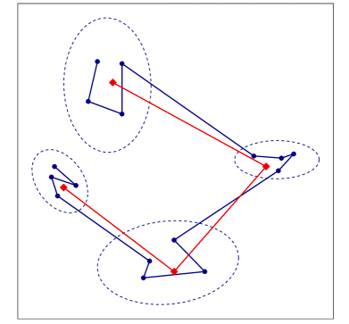
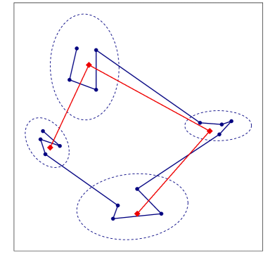
Figure 4: Illustration of condition (C). The points of $\bm{\theta}$ are depicted in blue ( $\bullet$) and the points of $\bm{\theta}_{0}$ are depicted in red ( ◆). The blue solid lines (—) denote the permutation $\alpha_{\bm{\theta}}$, while the red solid lines (—) denote the permutation $\alpha_{\bm{\theta}_{0}}$. The ellipses ( - - -) represent a choice of cluster partition of $\bm{\theta}$. The choice of cluster ordering in the left plot satisfies condition (C), while that of the right plot does not.

3.2 Main Results

We are now ready to state our main results. Theorem 1 below shows that $\{\widehat{\mathcal{V}}_{k}:1\leq k\leq K_{0}\}$ asymptotically forms a cluster partition of $\{\widehat{\bm{\theta}}_{1},\dots,\widehat{\bm{\theta}}_{K}\}$. This result, together with the rate of convergence established in Theorem 2, leads to the consistency of the GSF in estimating $K_{0}$, as stated in Theorem 3.

Theorem 1.

Assume conditions (SI), (A1)–(A2) and (F) hold, and let the penalty function $r_{\lambda_{n}}$ satisfy the following condition,

1. $r_{\lambda_{n}}(\eta;\omega)\geq 0$ is a nondecreasing function of $\eta\in\mathbb{R}_{+}$ which satisfies $r_{\lambda_{n}}(0;\omega)=0$ and $\lim_{n\to\infty}r_{\lambda_{n}}(\eta;\omega)=0$, for all $\eta,\omega\in\mathbb{R}_{+}$. Furthermore, for any fixed compact sets $I_{1},I_{2}\subseteq(0,\infty)$, $r_{\lambda_{n}}(\cdot;\omega)$ is convex over $I_{1}$ for large $n$, and $\mathrm{diam}(nr_{\lambda_{n}}(I_{1};I_{2}))=O(a_{n})$.

Then, as $n\to\infty$,

1. $W_{r}(\widehat{G}_{n},G_{0})\to 0$, almost surely, for all $r\geq 1$.

Assume further that condition (A3) holds. Then,

1. $\phi(\widehat{\pi}_{1},\dots,\widehat{\pi}_{K})=O_{p}(1)$. In particular, for every $k=1,\dots,K_{0}$, $\sum_{j\in\widehat{\mathcal{I}}_{k}}\widehat{\pi}_{j}=\pi_{0k}+o_{p}(1)$.

2. For every $1\leq l\leq K$, there exists a unique $1\leq k\leq K_{0}$, such that $\big{\lVert}\widehat{\bm{\theta}}_{l}-\bm{\theta}_{0k}\big{\rVert}=o_{p}(1),$ thus $\{\widehat{\mathcal{V}}_{k}:1\leq k\leq K_{0}\}$ is a cluster partition of $\{\widehat{\bm{\theta}}_{1},\dots,\widehat{\bm{\theta}}_{K}\}$, with probability tending to one.

Theorem 1.(i) establishes the consistency of $\widehat{G}_{n}$ under the Wasserstein distance—a property shared by the overfitted MLE $\bar{G}_{n}$ (Ho et al., 2016b, ). This is due to the fact that, by conditions (F) and (P1), the log-likelihood function is the dominant term in $L_{n}$, in (2.6). Theorem 1.(ii) implies that the estimated mixing proportions $\widehat{\pi}_{j}$ are stochastically bounded away from 0, which then results in Theorem 1.(iii) showing that every atom of $\widehat{G}_{n}$ is consistent in estimating an atom of $G_{0}$. A straightforward investigation of the proof shows that this property also holds for $\widetilde{G}_{n}$ in (3.7), but not for the overfitted MLE $\bar{G}_{n}$, which may have a subset of atoms whose limit points are not amongst those of $G_{0}$.

When $K>K_{0}$, the result of Theorem 1 does not imply the consistency of $\widehat{G}_{n}$ in estimating $K_{0}$. The latter is achieved if the number of distinct elements of each Voronoi cell $\widehat{\mathcal{V}}_{k}$ is equal to one with probability tending to one, which is shown in Theorem 3 below. To establish this result, we require an upper bound on the rate of convergence of $\widehat{G}_{n}$ under the Wasserstein distance. We obtain this bound by studying the rate of convergence of the density $p_{\widehat{G}_{n}}$ to $p_{0}$, with respect to the Hellinger distance, and appeal to inequality (3.2). van de Geer, (2000) (see also Wong et al., (1995)) established convergence rates for nonparametric maximum likelihood estimators under the Hellinger distance in terms of the bracket entropy integral

$$\mathcal{J}_{B}\left(\gamma,\bar{\mathcal{P}}_{K}^{\frac{1}{2}}(\gamma),\nu\right)=\int_{0}^{\gamma}\sqrt{H_{B}\left(u,\bar{\mathcal{P}}^{\frac{1}{2}}_{K}(u),\nu\right)}du,\quad\gamma>0,$$

where $H_{B}\big{(}u,\bar{\mathcal{P}}_{K}^{\frac{1}{2}}(u),\nu\big{)}$ denotes the $u$-bracket entropy with respect to the $L^{2}(\nu)$ metric of the density family

$$\bar{\mathcal{P}}_{K}^{\frac{1}{2}}(u)=\left\{\sqrt{\frac{p_{G}+p_{0}}{2}}:G\in\mathcal{G}_{K},\ h\left(\frac{p_{G}+p_{0}}{2},p_{0}\right)\leq u\right\},\quad u>0.$$

In our work, however, the main difficulty in bounding $h(p_{\widehat{G}_{n}},p_{0})$ is the presence of the penalty $r_{\lambda_{n}}$. The following Theorem shows that, as $n\to\infty$, if the growth rate of $r_{\lambda_{n}}$ away from zero, as a function of $\eta$, is carefully controlled, then $p_{\widehat{G}_{n}}$ achieves the same rate of convergence as the MLE $p_{\bar{G}_{n}}$.

Theorem 2.

Assume the same conditions as Theorem 1, and that the cluster ordering $\alpha_{\mathbf{t}}$ satisfies condition (C). For a universal constant $J>0$, assume there exists a sequence of real numbers $\gamma_{n}\gtrsim(\log n/n)^{1/2}$ such that for all $\gamma\geq\gamma_{n}$,

$$\mathcal{J}_{B}\left(\gamma,\bar{\mathcal{P}}_{K}^{\frac{1}{2}}(\gamma),\nu\right)\leq J\sqrt{n}\gamma^{2}.$$ (3.10)

Furthermore, assume $r_{\lambda_{n}}$ satisfies the following condition,

1. The restriction of $r_{\lambda_{n}}$ to any compact subset of $\{(\eta,\omega)\subseteq\mathbb{R}^{2}:\eta,\omega>0\}$ is Lipschitz continuous in both $\eta$ and $\omega$, with Lipschitz constant $\ell_{n}=O(\gamma_{n}^{3/2}/\log n)$, and $a_{n}\asymp n\ell_{n}\vee 1$.

Then, $h(p_{\widehat{G}_{n}},p_{0})=O_{p}(\gamma_{n}).$

Gaussian mixture models are known to satisfy condition (3.10) for $\gamma_{n}\asymp(\log n/n)^{\frac{1}{2}}$, under certain boundedness assumptions on $\Theta$ (Ghosal and van der Vaart,, 2001; Genovese et al.,, 2000). Lemma 3.2.1 of Ho, (2017) shows that (3.10) also holds for this choice of $\gamma_{n}$ for many of the strongly identifiable density families which we discuss below. For these density families, $p_{\widehat{G}_{n}}$ achieves the parametric rate of convergence up to polylogarithmic factors.

Let $\widehat{K}_{n}$ be the order of $\widehat{G}_{n}$, namely the number of distinct components $\widehat{\bm{\theta}}_{j}$ of $\widehat{G}_{n}$ with non-zero mixing proportions. We now prove the consistency of $\widehat{K}_{n}$ in estimating $K_{0}$.

Theorem 3.

Assume the same conditions as Theorem 2, and assume that the family $\mathcal{F}$ satisfies condition (A4). Suppose further that the penalty $r_{\lambda_{n}}$ satisfies the following condition,

1. $r_{\lambda_{n}}(\cdot;\omega)$ is differentiable for all $\omega>0$, and

   $$\lim_{n\to\infty}\inf\left\{\gamma_{n}^{-1}\ \frac{\partial r_{\lambda_{n}}(\eta;\omega)}{\partial\eta}:0<\eta\leq\gamma_{n}^{\frac{1}{2}}\log n,\ \omega\geq\left(\gamma_{n}^{\frac{\beta}{2}}\log n\right)^{-1}\right\}=\infty,$$

   where $\gamma_{n}$ is the sequence defined in Theorem 2, and $\beta>1$ is the constant in (3.8).

Then, as $n\to\infty$,

1. $\mathbb{P}(\widehat{K}_{n}=K_{0})\to 1.$ In particular, $\mathbb{P}\left(\bigcap_{k=1}^{K_{0}}\{|\widehat{\mathcal{V}}_{k}|=1\}\right)\to 1.$

2. $W_{1}(\widehat{G}_{n},G_{0})=O_{p}(\gamma_{n}).$

Condition (P3) ensures that as $n\to\infty$, $r_{\lambda_{n}}$ grows sufficiently fast in a vanishing neighborhood of $\eta=0$ to prevent any mixing measure of order greater than $K_{0}$ from maximizing $L_{n}$. In addition to being model selection consistent, Theorem 3 shows that for most strongly identifiable parametric families $\mathcal{F}$, $\widehat{G}_{n}$ is a $(\log n/n)^{1/2}$-consistent estimator of $G_{0}$. Thus, $\widehat{G}_{n}$ improves on the $(\log n/n)^{1/4}$ rate of convergence of the overfitted MLE $\bar{G}_{n}$. This fact combined with Theorem 1.(iii) implies that the fitted atoms $\widehat{\bm{\theta}}_{j}$ are also $(\log n/n)^{1/2}$-consistent in estimating the true atoms $\bm{\theta}_{0k}$, up to relabeling.

3.3 Remarks

We now discuss several aspects of the GSF in regards to the (SI) condition, penalty $r_{\lambda}$, upper bound $K$, and its relation to existing approaches in Bayesian mixture modeling.

(I) The Strong Identifiability (SI) Condition. A wide range of univariate parametric families are known to be strongly identifiable, including most exponential families (Chen,, 1995; Chen et al.,, 2004), and circular distributions (Holzmann et al.,, 2004). Strongly identifiable families with multidimensional parameter space include multivariate Gaussian distributions in location or scale, certain classes of Student-$t$ distributions, as well as von Mises, Weibull, logistic and Generalized Gumbel distributions (Ho et al., 2016b, ). In this paper, we also consider finite mixture of multinomial distributions. To establish conditions under which this family satisfies condition (SI), we begin with the following result.

Proposition 1.

Consider the binomial family with known number of trials $M\geq 1$,

$$\mathcal{F}=\left\{f(y;\theta)={{M}\choose y}\theta^{y}(1-\theta)^{M-y}:\theta\in(0,1),\ y\in\{0,\dots,M\}\right\}.$$ (3.11)

Given any integer $r\geq 1$, the condition $(r+1)K-1\leq M$ is necessary and sufficient for $\mathcal{F}$ to be strongly identifiable in the $r$-th order (Heinrich and Kahn,, 2018). That is, for any $K$ distinct points $\theta_{1},\dots,\theta_{K}\in(0,1)$, and $\beta_{jl}\in\mathbb{R}$, $j=1,\dots,K$, $l=0,\dots,r$, if

$$\sup_{y\in\{0,\dots,M\}}\left|\sum_{j=1}^{K}\sum_{l=0}^{r}\beta_{jl}\frac{\partial^{l}f(y;\theta_{j})}{\partial\theta^{l}}\right|=0,$$

then $\beta_{jl}=0$ for every $j=1,\dots,K$ and $l=0,\dots,r$.

The inequality $(r+1)K-1\leq M$ is comparable to the classical identifiability result of Teicher, (1963), which states that binomial mixture models are identifiable with respect to their mixing measure if and only if $2K-1\leq M$. Using Proposition 1, we can readily establish the following result.

Corollary 1.

A sufficient condition for the multinomial family

$$\textstyle\mathcal{F}=\left\{{{M}\choose{y_{1},\dots,y_{d}}}\prod_{j=1}^{d}\theta_{j}^{y_{j}}:\theta_{j}\in(0,1),\ 0\leq y_{j}\leq M,\ \sum_{j}^{d}\theta_{j}=1,\ \sum_{j}^{d}y_{j}=M\right\}$$ (3.12)

with known number of trials $M\geq 1$, to satisfy condition (SI) is $3K-1\leq M$.

(II) The Penalty Function $r_{\lambda_{n}}$. Condition (P1) is standard and is satisfied by most well-known regularization functions, including the Lasso, ALasso, SCAD and MCP, as long as $\lambda_{n}\to 0$, for large enough $a_{n}$, as $n\to\infty$. Conditions (P2) and (P3) are satisfied by SCAD and MCP when $\lambda_{n}\asymp\gamma_{n}^{\frac{1}{2}}\log n$. When $\gamma_{n}\asymp(\log n/n)^{1/2}$, it follows that $\lambda_{n}$ decays slower than the $n^{-1/4}$ rate, contrasting the typical rate $\lambda_{n}\asymp n^{-1/2}$ encountered in variable selection problems for parametric regression (see for instance Fan and Li, (2001)).

We now consider the ALasso with the weights $\omega_{j}$ in (3.8), which are similar to those proposed by Zou, (2006) in the context of variable selection in regression. Condition (P2) implies $\lambda_{n}\gamma_{n}^{-\frac{3}{2}}\log n\to 0$, while condition (P3) implies $\lambda_{n}\gamma^{-\frac{\beta+2}{2}}_{n}\to\infty$, where $\beta$ is the parameter in the weights. Thus, both conditions (P2) and (P3) are satisfied by the ALasso with the weights in (3.8) only when $\beta>1$ and by choosing $\lambda_{n}\asymp\gamma_{n}^{3/2}/\log n$. In particular, the value $\beta=1$ is invalid. When $\gamma_{n}\asymp(\log n/n)^{1/2}$, it follows that $\lambda_{n}\asymp n^{-3/4}(\log n)^{-1/4}$ which decays much faster than the sequence $\lambda_{n}$ required for the SCAD and MCP discussed above. This discrepancy can be anticipated from the fact the weights $\omega_{j}$ corresponding to nearby atoms of $\widetilde{G}_{n}$ diverge. It is worth noting that the typical tuning parameter for the ALasso in parametric regression is required to satisfy $\sqrt{n}\lambda_{n}\to 0$ and $n^{\frac{1+\beta}{2}}\lambda_{n}\to\infty$, for any $\beta>0$.

Finally, we note that the Lasso penalty $r_{\lambda_{n}}(\eta;\omega)=\lambda_{n}|\eta|$ cannot simultaneously satisfy conditions (P2) and (P3), since they would require opposing choices of $\lambda_{n}$. Furthermore, for this penalty, when $\Theta\subseteq\mathbb{R}$ and $\alpha$ is the natural ordering on the real line, that is $\theta_{\alpha(1)}\leq\dots\leq\theta_{\alpha(K)}$, we obtain the telescoping sum

$$\lambda_{n}\sum_{j=1}^{K-1}|\eta_{j}|=\lambda_{n}\sum_{j=1}^{K-1}(\theta_{\alpha(j+1)}-\theta_{\alpha(j)})=\lambda_{n}(\theta_{\alpha(K)}-\theta_{\alpha(1)})$$

which fails to penalize the vast majority of the overfitted components.

(III) Choice of the Upper Bound $K$. By Theorem 3, as long as the upper bound on the mixture order satisfies $K\geq K_{0}$, the GSF provides a consistent estimator of $K_{0}$. The following result shows the behaviour of the GSF for a misspecified bound $K<K_{0}$.

Proposition 2.

Assume that the family $\mathcal{F}$ satisfies condition (A3), and that the mixture family $\{p_{G}:G\in\mathcal{G}_{K}\}$ is identifiable, Then, for any $K<K_{0}$, as $n\to\infty$, the GSF order estimator $\widehat{K}_{n}$ satisfies: $\mathbb{P}(\widehat{K}_{n}=K)\to 1.$

Guided by the above result, if the GSF chooses the prespecified upper bound $K$ as the estimated order, the bound is likely misspecified and larger values should also be examined. This provides a natural heuristic for choosing an upper bound $K$ for the GSF in practice, which we further elaborate upon in Section 4.2 of the simulation study.

(IV) Connections between the GSF and Existing Bayesian Approaches. When $\varphi(\pi_{1},\dots,\pi_{K})=(1-\gamma)\sum_{j=1}^{K}\log\pi_{j}$, for some $\gamma>1$, the estimator $\widetilde{G}_{n}$ in (3.7) can be viewed as the posterior mode of the overfitted Bayesian mixture model

$$\bm{\theta}_{1},\dots,\bm{\theta}_{K}\leavevmode\nobreak\ \overset{\text{iid}}{\sim}\leavevmode\nobreak\ H,$$ (3.13)

$$(\pi_{1},\dots,\pi_{K})\leavevmode\nobreak\ \sim\leavevmode\nobreak\ \text{Dirichlet}\left(\gamma,\dots,\gamma\right),\leavevmode\nobreak\ \mathbf{Y}_{i}|G=\sum_{j=1}^{K}\pi_{j}\delta_{\bm{\theta}_{j}}\leavevmode\nobreak\ \leavevmode\nobreak\ \overset{\text{iid}}{\sim}\leavevmode\nobreak\ p_{G},\leavevmode\nobreak\ i=1,\dots,n,$$ (3.14)

where $H$ is a uniform prior on the (compact) set $\Theta\subseteq\mathbb{R}^{d}$. Under this setting, Rousseau and Mengersen, (2011) showed that when $\gamma<d/2$, the posterior distribution has the effect of asymptotically emptying out redundant components of the overfitted mixture model, such that the posterior expectation of the mixing probabilities of the $(K-K_{0}+1)$ extra components decay at the rate $n^{-1/2}$, up to polylogarithmic factors. On the other hand, if $\gamma>d/2$, two or more of the posterior atoms with non-negligible mixing probabilities will have the tendency to approach each other. The authors discuss that the former case results in more stable behaviour of the posterior distribution. In contrast, under our setting with the choice $\gamma>1$, Theorem 1.(i) implies that all the mixing probabilities of $\widetilde{G}_{n}$ are bounded away from zero with probability tending to one. This behaviour matches their above setting $\gamma>d/2$, though with a generally different cut-off for $\gamma$. We argue that the GSF does not suffer from the instability described by Rousseau and Mengersen, (2011) in this setting, as it proposes a simple procedure for merging nearby atoms using the second penalty $r_{\lambda}$ in (2.6), hinging upon the notion of cluster ordering. From a Bayesian standpoint, this penalty can be viewed as replacing the iid prior $H$ in (3.13) by the following exchangeable and non-iid prior

$$(\bm{\theta}_{1},\dots,\bm{\theta}_{K})\sim p_{\bm{\theta}}(\bm{\theta}_{1},\dots,\bm{\theta}_{K})\propto\prod_{j=1}^{K-1}\exp\Big{\{}-r_{\lambda}\big{(}\left\lVert\bm{\theta}_{\alpha_{\bm{\theta}}(j+1)}-\bm{\theta}_{\alpha_{\bm{\theta}}(j)}\right\rVert;\omega_{j}\big{)}\Big{\}}$$ (3.15)

up to rescaling of $r_{\lambda}$, which places high-probability mass on nearly-overlapping atoms. On the other hand, Petralia et al., (2012), Xie and Xu, (2020) replace $H$ by so-called repulsive priors, which favour diverse atoms, and are typically used with $\gamma<d/2$. For example, Petralia et al., (2012) study the prior

$$(\bm{\theta}_{1},\dots,\bm{\theta}_{K})\sim p_{\bm{\theta}}(\bm{\theta}_{1},\dots,\bm{\theta}_{K})\propto\prod_{j<k}^{K}\exp\left\{-\tau\left\lVert\bm{\theta}_{j}-\bm{\theta}_{k}\right\rVert^{-1}\right\},\quad\tau>0.$$ (3.16)

In contrast to the GSF, the choice $\gamma<d/2$ ensures vanishing posterior mixing probabilities corresponding to redundant components, which is further encouraged by the repulsive prior (3.16). Without a post-processing step which thresholds these mixing probabilities, however, this methods do not yield consistent order selection. It turns out that by further placing a prior on $K$, order consistency can be obtained (Nobile,, 1994; Miller and Harrison,, 2018).

A distinct line of work in nonparametric Bayesian mixture modeling places a prior, such as a Dirichlet process, directly on the mixing measure $G$. Though the resulting posterior typically has infinitely-many atoms, consistent estimators of $K_{0}<\infty$ can be obtained using post-processing techniques, such as the Merge-Truncate-Merge (MTM) method of Guha et al., (2019). Both the GSF and MTM aim at reducing the overfitted mixture order by merging nearby atoms. Unlike the GSF, however, the Dirichlet process mixture’s posterior may have vanishing mixing probabilities, hence a single merging stage of its atoms is insufficient to obtain an asymptotically correct order. The MTM thus also truncates such redundant components, and performs a second merging of their mixing probabilities to recover a proper mixing measure. Both the truncation and merging stages use hard-thresholding rules. We compare the two methods in our simulation study, Section 4.3.

4 Simulation Study

We conduct a simulation study to assess the finite-sample performance of the GSF. We develop a modification of the EM algorithm to obtain an approximate solution to the optimization problem in (2.7). The main ingredients are the Local Linear Approximation algorithm of Zou and Li, (2008) for nonconcave penalized likelihood models, and the proximal gradient method (Nesterov,, 2004). Details of our numerical solution are given in Supplement D.1. The algorithm is implemented in our R package GroupSortFuse.

In the GSF, the tuning parameter $\lambda$ regulates the order of the fitted model. Figure 1 (see also Figure 13 in Supplement E.7) shows the evolution of the parameter estimates $\widehat{\bm{\theta}}_{j}(\lambda)$ for a simulated dataset, over a grid of $\lambda$-values. These qualitative representations can provide insight about the order of the mixture model, for purposes of exploratory data analysis. For instance, as seen in the figures, when small values of $\lambda$ lead to a significant reduction in the postulated order $K$, a tighter bound on $K_{0}$ can often be obtained. In applications where a specific choice of $\lambda$ is required, common techniques include $v$-fold Cross Validation and the BIC, applied directly to the MPLE for varying values of $\lambda$ (Zhang et al., 2010b, ). In our simulation, we use the BIC due to its low computational burden.

Default Choices of Penalties, Tuning Parameters, and Cluster Ordering. Throughout all simulations and real data analyses in this paper, including those contained in Figures 1-3, the following choices were used by default unless otherwise specified. We used the penalty $\varphi(\pi_{1},\dots,\pi_{K})=(1-\gamma)\sum_{j=1}^{K}\log\pi_{j}$, with the constant $1-\gamma\approx-\log 20$ following the suggestion of Chen and Kalbfleisch, (1996). The penalty $r_{\lambda}$ is taken to be the SCAD by default, though we also consider simulations below which employ the MCP and ALasso penalties. For the ALasso, the weights $\omega_{j}$ are specified as in (3.8). The tuning parameter $\lambda$ is selected using the BIC as described above. The cluster ordering $\alpha_{\bm{\theta}}$ is chosen as in (2.5). We recall that this choice does not constrain $\alpha_{\bm{\theta}}(1)$—in our simulations, we chose this value using a heuristic which ensures that $\alpha_{\bm{\theta}}$ reduces to the natural ordering on $\mathbb{R}$ in the case $d=1$. Further numerical details are given in Supplement D.2.

4.1 Parameter Settings and Order Selection Results

Our simulations are based on multinomial and multivariate location-Gaussian mixture models. We compare the GSF under the SCAD (GSF-SCAD), MCP (GSF-MCP) and ALasso (GSF-ALasso) penalties to the AIC, BIC, and ICL (Biernacki et al.,, 2000), as implemented in the R packages mixtools (Benaglia et al.,, 2009) and mclust (Fraley and Raftery,, 1999). ICL performed similarly to the BIC in our multinomial simulations, but generally underperformed in our Gaussian simulations. Therefore, below we only discuss the performance of AIC and BIC.

We report the proportion of times that each method selected the correct order $K_{0}$, out of 500 replications, based on the models described below. For each simulation, we also report detailed tables in Supplement E with the number of times each method incorrectly selected orders other than $K_{0}$. We fix the upper bound $K=12$ throughout this section. For this choice, the effective number of parameters of the mixture models hereafter is less than the smallest sample sizes considered.

Multinomial Mixture Models. The density function of multinomial mixture model of order $K$ is given by

$$p_{G}(\mathbf{y})=\sum_{j=1}^{K}\pi_{j}{{M}\choose{y_{1},\dots,y_{d}}}\prod_{l=1}^{d}\theta_{jl}^{y_{l}}$$ (4.1)

with $\bm{\theta}_{j}=(\theta_{j1},\dots,\theta_{jd})^{\top}\in(0,1)^{d}$, $\mathbf{y}=(y_{1},\dots,y_{d})^{\top}\in\{1,\dots,M\}^{d}$, where $\sum_{l=1}^{d}\theta_{jl}=1$, $\sum_{l}^{d}y_{l}=M$. We consider 7 models with true orders $K_{0}=2,3,...,8$, dimensions $d=3,4,5$, and $M=35,50$ to satisfy the strong identifiability condition $3K-1\leq M$ described in Corollary 1. The parameter settings are given in Table 1. The results for $M=50$ are reported in Figure 4.1 below. Those for $M=35$ are similar, and are relegated to Supplement E.1. The simulation results are based on the sample sizes $n=100,200,400$.

Model	1	2	3
$\pi_{1},\bm{\theta}_{1}$	$.2,(.2,.2,.2,.2,.2)$	$\frac{1}{3},(.2,.2,.2,.2,.2)$	$.25,(.2,.2,.6)$
$\pi_{2},\bm{\theta}_{2}$	$.8,(.1,.3,.2,.1,.3)$	$\frac{1}{3},(.1,.3,.2,.1,.3)$	$.25,(.2,.6,.2)$
$\pi_{3},\bm{\theta}_{3}$		$\frac{1}{3},(.3,.1,.2,.3,.1)$	$.25,(.6,.2,.2)$
$\pi_{4},\bm{\theta}_{4}$			$.25,(.45,.1,.45)$

Model	4	5	6	7
$\pi_{1},\bm{\theta}_{1}$	$.2,(.2,.2,.6)$	$\frac{1}{6},(.2,.2,.6)$	$\frac{1}{7},(.2,.2,.6)$	$.125,(.2,.2,.2,.4)$
$\pi_{2},\bm{\theta}_{2}$	$.2,(.6,.2,.2)$	$\frac{1}{6},(.2,.6,.2)$	$\frac{1}{7},(.2,.6,,2)$	$.125,(.2,.2,.4,.2)$
$\pi_{3},\bm{\theta}_{3}$	$.2,(.45,.1,.45)$	$\frac{1}{6},(.6,.2,.2)$	$\frac{1}{7},(.6,.2,.2)$	$.125,(.2,.4,.2,.2)$
$\pi_{4},\bm{\theta}_{4}$	$.2,(.2,.7,.1)$	$\frac{1}{6},(.45,.1,.45)$	$\frac{1}{7},(.45,.1,.45)$	$.125,(.4,.2,.2,.2)$
$\pi_{5},\bm{\theta}_{5}$	$.2,(.1,.7,.2)$	$\frac{1}{6},(.2,.7,.1)$	$\frac{1}{7},(.1,.7,.2)$	$.125,(.1,.3,.1,.5)$
$\pi_{6},\bm{\theta}_{6}$		$\frac{1}{6},(.1,.7,.2)$	$\frac{1}{7},(.7,.2,.1)$	$.125,(.1,.3,.5,.1)$
$\pi_{7},\bm{\theta}_{7}$			$\frac{1}{7},(.1,.2,.7)$	$.125,(.1,.5,.3,.1)$
$\pi_{8},\bm{\theta}_{8}$				$.125,(.5,.1,.3,.1)$

Table 1: Parameter settings for the multinomial mixture Models 1–7.

Under Model 1, all five methods selected the correct order most often, and exhibited similar performance across all the sample sizes—the results are reported in Table 4 of Supplement E.1. The results for Models 2-7 with orders $K_{0}=2,3,4,5$, are plotted by percentage of correctly selected orders in Figure 4.1. Under Model 2, the correct order is selected most frequently by the BIC and GSF-ALasso, for all the sample sizes. Under Models 3 and 4, the GSF with all three penalties, in particular the GSF-ALasso, outperforms AIC and BIC. Under Models 5-7, all methods selected the correct order for $n=100$ fewer than 55% of the time. For $n=200$, the GSF-SCAD and GSF-MCP select the correct number of components more than 55% of the time, unlike AIC and BIC. All three GSF penalties continue to outperform the other methods when $n=400$.

figure Percentage of correctly selected orders for the multinomial mixture models.

Multivariate Location-Gaussian Mixtures with Unknown Covariance Matrix. The density function of a multivariate Gaussian mixture model in mean, of order $K$, is given by

Model	$\sigma_{ij}$	$\pi_{1},\bm{\mu}_{1}$	$\pi_{2},\bm{\mu}_{2}$	$\pi_{3},\bm{\mu}_{3}$	$\pi_{4},\bm{\mu}_{4}$	$\pi_{5},\bm{\mu}_{5}$
1.a	$I(i=j)$	$.5,(0,0)^{\top}$	.5, $(2,2)^{\top}$
1.b	$(0.5)^{|i-j|}$	$.5,(0,0)^{\top}$	.5, $(2,2)^{\top}$
2.a	$I(i=j)$	$.25,(0,0)^{\top}$	$.25,(2,2)^{\top}$	$.25,(4,4)^{\top}$	$.25,(6,6)^{\top}$
2.b	$(0.5)^{|i-j|}$	$.25,(0,0)^{\top}$	$.25,(2,2)^{\top}$	$.25,(4,4)^{\top}$	$.25,(6,6)^{\top}$
$\begin{matrix}\text{3.a}\\ \text{3.b}\end{matrix}$	$\begin{matrix}I(i=j)\\ (0.5)^{|i-j|}\end{matrix}$	$\frac{1}{3},\begin{pmatrix}0\\ 0\\ 0\\ 0\end{pmatrix}$	$\frac{1}{3},\begin{pmatrix}2.5\\ 1.5\\ 2\\ 1.5\end{pmatrix}$	$\frac{1}{3},\begin{pmatrix}1.5\\ 3\\ 2.75\\ 2\end{pmatrix}$
$\begin{matrix}\text{4.a}\\ \text{4.b}\end{matrix}$	$\begin{matrix}I(i=j)\\ (0.5)^{|i-j|}\end{matrix}$	$\frac{1}{5},\begin{pmatrix}0\\ 0\\ 0\\ 0\\ 0\\ 0\end{pmatrix}$	$\frac{1}{5},\begin{pmatrix}-1.5\\ 2.25\\ -1\\ 0\\ .5\\ .75\end{pmatrix}$	$\frac{1}{5},\begin{pmatrix}.25\\ 1.5\\ .75\\ .25\\ -.5\\ -1\end{pmatrix}$	$\frac{1}{5},\begin{pmatrix}-.25\\ .5\\ -2.5\\ 1.25\\ .75\\ 1.5\end{pmatrix}$	$\frac{1}{5},\begin{pmatrix}-1\\ -1.5\\ -.25\\ 1.75\\ -.5\\ 2\end{pmatrix}$
$\begin{matrix}\text{5.a}\\ \text{5.b}\end{matrix}$	$\begin{matrix}I(i=j)\\ (0.5)^{|i-j|}\end{matrix}$	$\frac{1}{5},\begin{pmatrix}0\\ 0\\ 0\\ 0\\ 0\\ 0\\ 0\\ 0\end{pmatrix}$	$\frac{1}{5},\begin{pmatrix}1\\ 1.5\\ 0.75\\ 2\\ 1.5\\ 1.75\\ 0.5\\ 2.5\end{pmatrix}$	$\frac{1}{5},\begin{pmatrix}2\\ 0.75\\ 1.5\\ 1\\ 1.75\\ 0.5\\ 2.5\\ 1.5\end{pmatrix}$	$\frac{1}{5},\begin{pmatrix}1.5\\ 2\\ 1\\ 0.75\\ 2.5\\ 1.5\\ 1.75\\ 0.5\end{pmatrix}$	$\frac{1}{5},\begin{pmatrix}0.75\\ 1\\ 2\\ 1.5\\ 0.5\\ 2.5\\ 1.5\\ 1.75\end{pmatrix}$

Table 2: Parameter settings for the multivariate Gaussian mixture models.

$$p_{G}(\mathbf{y})=\sum_{j=1}^{K}\pi_{j}\frac{1}{\sqrt{(2\pi)^{d}|\bm{\Sigma}}|}\exp\left\{-\frac{1}{2}(\mathbf{y}-\bm{\mu}_{j})^{\top}\bm{\Sigma}^{-1}(\mathbf{y}-\bm{\mu}_{j})\right\},$$

where $\bm{\mu}_{j}\in\mathbb{R}^{d},j=1,\dots,K$, and $\bm{\Sigma}=\{\sigma_{ij}:i,j=1,\ldots,d\}$ is a positive definite $d\times d$ covariance matrix. We consider the 10 mixture models in Table 2 with true orders $K_{0}=2,3,4,5$, and with dimension $d=2,4,6,8$. For each model, we consider both an identity and non-identity covariance matrix $\bm{\Sigma}$, which is estimated as an unknown parameter. The simulation results are based on the sample sizes $n=200,400,600,800$.

The results for Models 1.a, 1.b, 3.a, 3.b, 4.a, 4.b are plotted by percentage of correctly selected orders in Figure 5 below. Detailed results for the more challenging Models 2.a, 2.b, 5.a and 5.b are reported by percentage of selected orders between $1,\dots,K(=12)$ in Tables 18 and 21 of Supplement E.2.

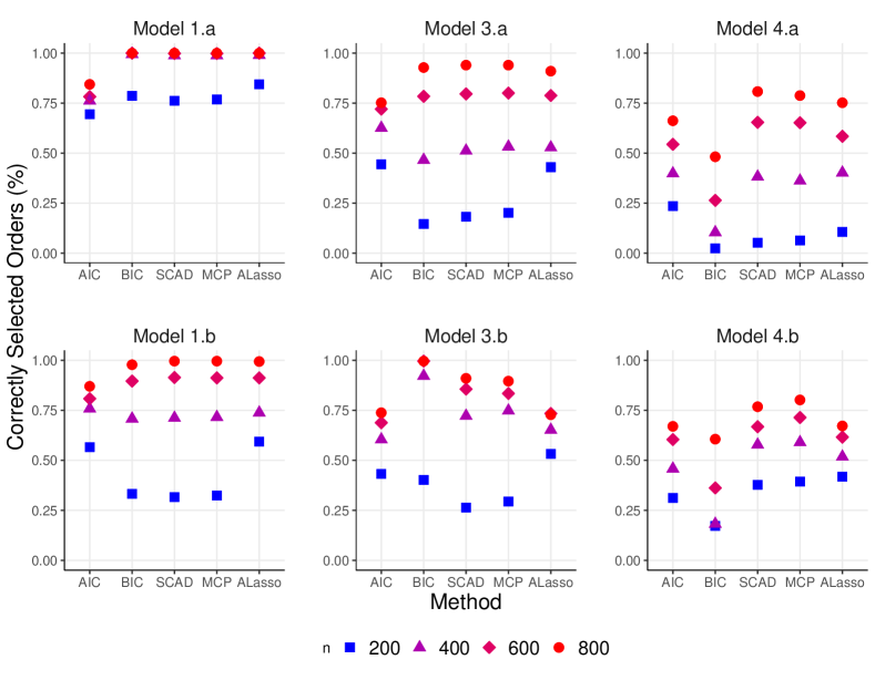
Figure 5: Percentage of correctly selected orders for the multivariate Gaussian mixture models.

In Figure 5, under Models 1.a and 1.b with $d=2$, all the methods selected the correct number of components most frequently for $n=400,600,800$; however, the performance of all methods deteriorates in Model 1.b with non-identity covariance matrix when $n=200$. Under Model 3.a with $d=4$, all methods perform similarly for $n=400,600,800$, but the GSF-ALasso and the AIC outperformed the other methods for $n=200$. Under Model 3.b, the BIC outperformed the other methods for $n=400,600,800$, but the GSF-ALasso again performed the best for $n=200$. In Models 4.a and 4.b with $d=6$, the GSF with the three penalties outperformed AIC and BIC across all sample sizes.

From Table 18, under Model 2.a with $d=2$ and identity covariance matrix, the BIC and the GSF with the three penalties underestimate and the AIC overestimates the true order, for sample sizes $n=200,400$. The three GSF penalties significantly outperform the AIC and BIC, when $n=600,800$. For the more difficult Model 2.b with non-identity covariance matrix, all methods underestimate across all sample sizes considered, but the AIC selects the correct order most frequently. From Table 21, under Model 5.a, all methods apart from AIC underestimated $K_{0}$ for $n=200,400,600$, and the three GSF penalties outperformed the other methods when $n=800$. Interestingly, the performance of all methods improves for Model 5.b with non-identity covariance matrix. Though all methods performed well for $n=400,600,800$, the BIC did so the best, while the GSF-ALasso exhibited the best performance when $n=200$.

In summary, depending on the models and sample sizes considered here, in some cases AIC or BIC exhibit the best performance, while in others the GSF based on at least one of the penalties (ALasso, SCAD, or MCP) outperforms. The universality of information criteria in almost any model selection problem is in part due to their ease of use on the investigator’s part, while many other methods require specification of multiple tuning parameters. Though we defined the GSF in its most general form, our empirical investigation suggests that, other than $\lambda$ and $K$, its tuning parameters ($\alpha_{\mathbf{t}},\varphi,\omega_{j}$, and choices therein) may not need to be tuned beyond their default choices used here. We have shown that off-the-shelf data-driven methods for selecting $\lambda$ yield reasonable performance. We next discuss the choice of the bound $K$.

4.2 Sensitivity Analysis for the Upper Bound $K$

In this section, we assess the sensitivity of the GSF with respect to the choice of upper bound $K$ via simulation. Specifically, we show the behaviour of the GSF for a range of $K$-values which are both misspecified ($K<K_{0}$) and well-specified ($K\geq K_{0}$). In the former case, by Proposition 2, the GSF is expected to select the order $K$, whereas in the latter case, by Theorem 3, the GSF selects the correct $K_{0}$ with high probability.

We consider the multinomial Models 3 ($K_{0}=4$) and 5 ($K_{0}=6$) with sample size $n=400$, and the Gaussian Models 3.a ($K_{0}=3$) and 4.a ($K_{0}=5$) with sample size $n=600$. The results are based on $80$ simulated samples from each model. For each sample, we apply the GSF-SCAD with $K=2,\ldots,25$, and then report the most frequently estimated order $\widehat{K}$, as well as the average estimated order over the $80$ samples. The results are given in Figure 6. Detailed results are reported by percentage of selected orders with respect to the bounds $K=2,\dots,25$, in Tables 22-25 of Supplement E.3.

For all four models, it can be seen that the GSF estimates the order $K$ most frequently when $K<K_{0}$. In fact, it does so on every replication for $K=1,2$ (resp. $K=1,2,3$) under multinomial Model 3 (resp. Model 5). When $K\geq K_{0}$, the GSF correctly estimates the order $K_{0}$ most frequently for all four models. Although the average selected order is seen to slightly deviate from $K_{0}$ as $K$ increases (as was already noted in Figure 3), the overall behaviour of the GSF is remarkably stable with respect to the choice of $K$. The resulting elbow shape of the solid red lines in Figure 6 is anticipated by Theorem 3 and Proposition 2.

Guided by the above results, in applications where finite mixture models ($K_{0}<\infty$) have meaningful interpretations in capturing population heterogeneity, we suggest to examine the GSF over a range of small to large values of $K$. This range may be chosen with consideration of the resulting number of mixture parameters, with respect to the sample size $n$. An elbow-shaped scatter plot of $(K,\widehat{K})$ can shed light on a safe choice of the bound $K$ and the selected order $\widehat{K}$. We illustrate such a strategy through the real data analysis in Section 5.

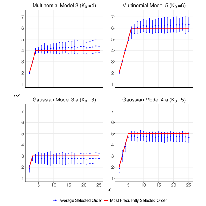
Figure 6: Sensitivity analysis of the GSF with respect to the upper bound $K$. Error bars represent one standard deviation of the fitted order.

4.3 Comparison of Merging-Based Methods

We now compare the GSF to alternate order selection methods which are also based on merging the components of an overfitted mixture. Our simulations are based on location-Gaussian mixture models, though unlike Section 4.1, we now treat the common covariance $\bm{\Sigma}$ as known. In addition to the GSF, and to the AIC/BIC which are included as benchmarks, we consider the following two methods.

1. The Merge-Truncate-Merge (MTM) procedure (Guha et al.,, 2019) described in Section 3.3(IV), applied to posterior samples from a Dirichlet Process mixture (DPM).

2. A hard-thresholding analogue of the GSF, denote by GSF-Hard, which is obtained by first computing the estimator $\widetilde{G}_{n}$ in (2.3), and then merging the atoms of $\widetilde{G}_{n}$ which fall within a sufficiently small distance $\lambda>0$ of each other (see Algorithm 2 in Supplement D.2 for a precise description). The GSF-Hard thus replaces the penalty $r_{\lambda}$ in the GSF with a post-hoc merging rule. By a straightforward simplification of our asymptotic theory, the GSF-Hard estimator satisfies the same properties as $\widehat{G}_{n}$ in Theorems 1–3.

We fit the MTM procedure using the same algorithm and parameter settings as described in Section 5 of Guha et al., (2019). The truncation and (second) merging stages of the MTM require a tuning parameter $c>0$, which plays a similar role as $\lambda$ in the GSF-Hard. The authors recommend considering various choices of $c$ in practice, though we are not aware of a method for tuning $c$. We therefore follow them by reporting the performance of the MTM for a range of $c$-values. For the GSF-Hard, we tune $\lambda$ using the BIC. Further implementation details are provided in Supplement D.2.

We report the proportion of times that each method selected the correct order under Gaussian Models 1.b and 2.a in Figure 7, based on $n=50,100,200,400$. More detailed results can be found in Supplement E.4, including those for $n=600,800$. For each sample size, we perform 80 replications due to the computational burden associated with fitting Dirichlet Process mixture models. The MTM results are based on the posterior mode.

The AIC, BIC, and GSF under all three penalties exhibit improved performance under the current setting with fixed $\bm{\Sigma}$, compared to that of Section 4.1. The GSF-Hard performs reasonably under Model 1.b but markedly underperforms in Model 2.a. Regarding the MTM, we report the results under four consecutive $c$-values which were most favourable from a range of 16 candidate values. Under Model 1.b, the MTM under all four $c$-values estimates $K_{0}$ most of the time, under most sample sizes, but underperforms compared to the remaining methods. In contrast, under Model 2.a, there exists a value of $c$ for which the MTM remarkably estimates $K_{0}$ on nearly all replications. However, the sensitivity to $c$ is also seen to increase, which can be problematic in the absence of a data-driven tuning procedure. Finally, we recall that the MTM is based on a nonparametric Bayes procedure, while the other methods are parametric and might generally require smaller sample sizes to achieve reasonable accuracy.

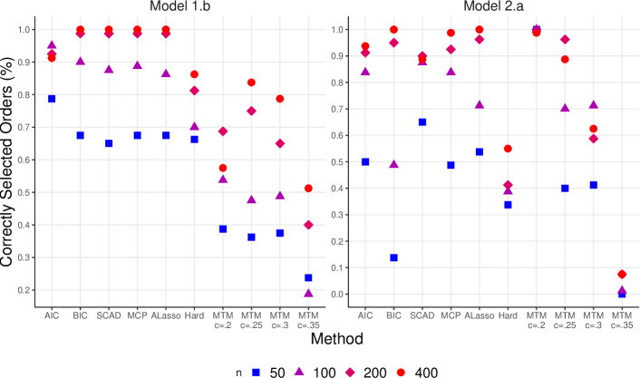
Figure 7: Percentage of correctly selected orders for the multivariate Gaussian models with common and known covariance matrix.

We emphasize that MTM and GSF-Hard are both post-hoc procedures for reducing the order of an overfitted mixing measure $G_{n}$, which is respectively equal to a sample from the DPM posterior, or to the estimator $\widetilde{G}_{n}$. This contrasts the GSF, which uses continuous penalties of the parameters to simultaneously perform order selection and mixing measure estimation, and does not vary discretely with the tuning parameter $\lambda$. On the other hand, these two post-hoc procedures have the practical advantage of being computationally inexpensive wrappers on top of the well-studied estimators $G_{n}$, for which standard implementations are available. To illustrate this point, in Table 3 we report the computational time associated with the results from Figure 7, including also the sample sizes $n=600,800$. It can be seen that GSF-Hard is typically computable with an order of magnitude fewer seconds than the GSF under any of the three penalties. The computational times for the MTM are largely dominated by the time required to sample the DPM posterior with the implementation we used—the post-processing procedure itself accounts for a negligible fraction of this time.

	Model 1.b						Model 2.a
$n$	AIC/ BIC	GSF-SCAD	GSF-MCP	GSF-ALasso	GSF-Hard	MTM	AIC/ BIC	GSF-SCAD	GSF-MCP	GSF-ALasso	GSF-Hard	MTM
50	23.6	1.30	1.2	5.3	3.8	2830.0	21.1	2.6	1.8	5.3	3.9	2502.6
100	29.8	2.7	2.0	9.9	5.2	7148.2	25.6	6.3	3.8	9.9	5.4	5607.2
200	38.7	6.7	4.5	19.6	6.8	25428.3	34.9	17.2	8.6	19.6	7.0	21008.0
400	47.6	12.4	8.5	35.8	7.6	34911.9	45.8	43.5	16.4	35.8	9.0	20151.2
600	54.4	24.2	15.3	49.3	8.8	51131.0	51.3	57.8	21.8	49.3	10.0	37535.7
800	60.0	32.2	22.8	67.1	9.9	74185.0	56.7	103.6	39.9	67.1	10.3	57469.7

Table 3: Average computational time (in seconds) per replication for the multivariate Gaussian models with common and known covariance matrix.

5 Real Data Example

We consider the data analyzed by Mosimann, (1962), arising from the study of the Bellas Artes pollen core from the Valley of Mexico, in view of reconstructing surrounding vegetation changes from the past. The data consists of $M=100$ counts on the frequency of occurrence of $d=4$ kinds of fossil pollen grains, at $n=73$ different levels of a pollen core. A simple multinomial model provides a poor fit to this data, due to over-dispersion caused by clumped sampling. Mosimann, (1962) modelled this extra variation using a Dirichlet-multinomial distribution, and Morel and Nagaraj, (1993) fitted a 3-component multinomial mixture model.

We applied the GSF-SCAD with upper bounds $K=2,\ldots,25$. For each $K$, we fitted the GSF based on five different initial values for the modified EM algorithm, and selected the model with optimal tuning parameter value. For $K=2$, the estimated order was $2$ and for $K\geq 3$, the most frequently selected order was $\widehat{K}=3$. Given the similarity of the sample size and dimension with those considered in the simulations, below we report the fitted model corresponding to the upper bound $K=12$.

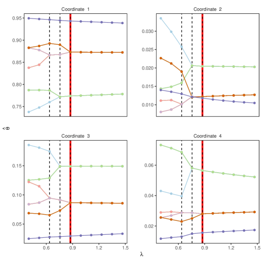
Figure 8: Coefficient plots for the GSF-SCAD on the pollen data. The vertical red lines indicate the selected tuning parameter.

The models obtained by the GSF with the three penalties are similar—for instance, the fitted model obtained by the GSF-SCAD is

$$.15\leavevmode\nobreak\ \text{Mult}(\widehat{\bm{\theta}}_{1})+.25\leavevmode\nobreak\ \text{Mult}(\widehat{\bm{\theta}}_{2})+.60\leavevmode\nobreak\ \text{Mult}(\widehat{\bm{\theta}}_{3}).$$

where $\text{Mult}(\bm{\theta})$ denotes the multinomial distribution with 100 trials and probabilities $\bm{\theta}$, $\widehat{\bm{\theta}}_{1}=(.94,.01,.03,.02)^{\top}$, $\widehat{\bm{\theta}}_{2}=(.77,.02,.15,.06)^{\top}$ and $\widehat{\bm{\theta}}_{3}=(.87,.01,.09,.03)^{\top}$. The log-likelihood value for this estimate is -499.87. The coefficient plots produced by the tuning parameter selector for GSF-SCAD are shown in Figure 8. Interestingly, the fitted order equals 3, for all $\lambda>0.9$ in the range considered, coinciding with the final selected order, and with the aforementioned sensitivity analysis on $K$.

We also ran the AIC, BIC and ICL on this data. The AIC selected six components, while the BIC and ICL selected three components. The fitted model under the latter two methods is given by

$$.17\leavevmode\nobreak\ \text{Mult}(\widehat{\bm{\theta}}_{1})+.22\leavevmode\nobreak\ \text{Mult}(\widehat{\bm{\theta}}_{2})+.61\leavevmode\nobreak\ \text{Mult}(\widehat{\bm{\theta}}_{3}).$$

where $\widehat{\bm{\theta}}_{1}=(.95,.02,.03,.01)^{\top}$, $\widehat{\bm{\theta}}_{2}=(.77,.02,.15,.07)^{\top}$ and $\widehat{\bm{\theta}}_{3}=(.87,.01,.09,.03)^{\top}$, with entries rounded to the nearest hundredths. The log-likelihood value for this estimate is -496.39.

6 Conclusion and Discussion

In this paper, we developed the Group-Sort-Fuse (GSF) method for estimating the order of finite mixture models with a multidimensional parameter space. By starting with a conservative upper bound $K$ on the mixture order, the GSF estimates the true order by applying two penalties to the overfitted log-likelihood, which group and fuse redundant mixture components. Under certain regularity conditions, the GSF is consistent in estimating the true order and it further provides a $\sqrt{n}$-consistent estimator for the true mixing measure (up to polylogarithmic factors). We examined its finite sample performance via thorough simulations, and illustrated its application to two real datasets, one of which is relegated to Supplement E.6.

We suggested the use of off-the-shelf methods, such as $v$-fold cross validation or the BIC, for selecting the tuning parameter $\lambda_{n}$ involved in the penalty $r_{\lambda_{n}}$. Properties of such choices with respect to our theoretical guidelines, or alternative methods specialized to the GSF, require further investigation.

The methodology developed in this paper may be applicable to mixtures which satisfy weaker notions of strong identifiability (Ho et al., 2016a, ). Extending our proof techniques to such models is, however, nontrivial. In particular, bounding the log-likelihood ratio statistic for the overfitted MLE $\bar{G}_{n}$ (Dacunha-Castelle et al.,, 1999), and the penalized log-likelihood ratio for the MPLE $\widehat{G}_{n}$, would require new insights in the absence of (second-order) strong identifiability. Empirically, we illustrated in Section 4.1 the promising finite sample performance of the GSF under location-Gaussian mixtures with an unknown but common covariance matrix, which themselves violate condition (SI).

We have shown that the GSF achieves a near-parametric rate of convergence under the Wasserstein distance, but this rate only holds pointwise in the true mixing measure $G_{0}$. Our work leaves open the behaviour of the GSF when the true mixing measure is permitted to vary with the sample size $n$—indeed, the minimax risk is known to scale at a rate markedly slower than parametric (Heinrich and Kahn,, 2018; Wu et al.,, 2020).

We established in Proposition 2 the asymptotic behaviour of the GSF when the upper bound $K$ is underspecified. However, our work provides no guarantees when other aspects of the mixture model $\mathcal{P}_{K}=\{p_{G}:G\in\mathcal{G}_{K}\}$ are misspecified, such as the kernel density family $\mathcal{F}$. We note that the recent work of Guha et al., (2019) establishes the asymptotic behaviour of various Bayesian procedures under such misspecification, in terms of a suitable Kullback-Leibler projection of the true mixture distribution. While we expect the GSF to obey similar asymptotics, we are not aware of a general theory for maximum likelihood estimation under misspecification in non-convex models such as $\mathcal{P}_{K}$. We leave a careful investigation of such properties to future work.

We believe that the framework developed in this paper paves the way to a new class of methods for order selection problems in other latent-variable models, such as mixture of regressions and Markov-switching autoregressive models (Frühwirth-Schnatter,, 2006). Results of the type developed by Dacunha-Castelle et al., (1999) in understanding large sample behaviour of likelihood ratio statistics for these models, and the recent work of Ho et al., (2019) in characterizing rates of convergence for parameter estimation in over-specified Gaussian mixtures of experts, may provide first steps toward such extensions. We also mention applications of the GSF procedure to non-model-based clustering methods, such as the $K$-means algorithm. While the notion of order, or true number of clusters, is generally elusive in the absence of a model, extensions of the GSF may provide a natural heuristic for choosing the number of clusters in such methods.

Acknowledgements. We would like to thank the editor, an associate editor, and two referees for their insightful comments and suggestions which significantly improved the quality of this paper. We thank Jiahua Chen for discussions related to the proof of Proposition 1, Russell Steele for bringing to our attention the multinomial dataset analyzed in Section 5, and Aritra Guha for sharing an implementation of the Merge-Truncate-Merge procedure. We also thank Sivaraman Balakrishnan and Larry Wasserman for useful discussions. Tudor Manole was supported by the Natural Sciences and Engineering Research Council of Canada and also by the Fonds de recherche du Québec–Nature et technologies. Abbas Khalili was supported by the Natural Sciences and Engineering Research Council of Canada through Discovery Grant (nserc rgpin-2015-03805 and nserc rgpin-2020-05011).

Supplementary Material

This Supplementary Material contains six sections. Supplement A contains notation which will be used throughout the sequel. Supplement B states several results from other papers which are needed for our subsequent proofs. Supplement C contains all proofs of the results stated in the paper, and includes the statements and proofs of several auxiliary results. Supplement D outlines our numerical solution, and Supplement E reports several figures and tables cited in the paper. Finally, Supplement F reports the implementation and complete numerical results of the simulation in Figure 3 of the paper.

Supplement A: Notation

Recall that $\mathcal{F}=\{f(\mathbf{y};\bm{\theta}):\bm{\theta}=(\theta_{1},\theta_{2},\ldots,\theta_{d})^{\top}\in\Theta\subseteq\mathbb{R}^{d},\ \mathbf{y}\in\mathcal{Y}\subseteq\mathbb{R}^{N}\}$ is a parametric density family with respect to a $\sigma$-finite measure $\nu$. Let

$$\mathcal{P}_{K}=\left\{p_{G}(\mathbf{y})=\int_{\Theta}f(\mathbf{y};\bm{\theta})dG(\bm{\theta}):G\in\mathcal{G}_{K}\right\},$$ (S.1)

where, recall, that $\mathcal{G}_{K}$ is the set of finite mixing measures with order at most $K\geq K_{0}$. Let $p_{0}=p_{G_{0}}$ be the density of the true finite mixture model with its corresponding probability distribution $P_{0}$. Let $\widehat{p}_{n}=p_{\widehat{G}_{n}}$ be the estimated mixture density based on the MPLE $\widehat{G}_{n}$, and define the empirical measure $P_{n}=\frac{1}{n}\sum_{i=1}^{n}\delta_{\mathbf{Y}_{i}}$.

For any $p_{G}\in\mathcal{P}_{K}$, let $\bar{p}_{G}=\frac{p_{G}+p_{0}}{2}$, and $\bar{\mathcal{P}}_{K}^{\frac{1}{2}}=\left\{\bar{p}_{G}^{\frac{1}{2}}:p_{G}\in\mathcal{P}_{K}\right\}$. For any $\delta>0$, recall that

$$\bar{\mathcal{P}}_{K}^{\frac{1}{2}}(\delta)=\left\{\bar{p}_{G}^{\frac{1}{2}}\in\bar{\mathcal{P}}_{K}^{\frac{1}{2}}:h(\bar{p}_{G},p_{0})\leq\delta\right\}.$$

Furthermore, define the empirical process

$$\nu_{n}(G)=\sqrt{n}\int_{\{p_{0}>0\}}\frac{1}{2}\log\bigg{\{}\frac{p_{G}+p_{0}}{2p_{0}}\bigg{\}}d(P_{n}-P_{0}),\quad G\in\mathcal{G}_{K}.$$ (S.2)

We also define the following two collections of mixing measures, for some $0<b_{0}<1$,

$$\mathcal{G}_{K}(b_{0}) =\left\{G\in\mathcal{G}_{K}\setminus\mathcal{G}_{K_{0}-1}:G=\sum_{j=1}^{K}\pi_{j}\delta_{\bm{\theta}_{j}},\ \pi_{j}\geq b_{0}\right\},$$ (S.3)

$$\mathcal{G}_{K}(b_{0};\gamma) =\left\{G\in\mathcal{G}_{K}(b_{0}):h(p_{G},p_{G_{0}})\leq\gamma\right\},\quad\forall\gamma>0.$$ (S.4)

Also, let

$$\text{KL}(p,q)=\int\log\left(\frac{p}{q}\right)\leavevmode\nobreak\ p\leavevmode\nobreak\ d\nu$$ (S.5)

denote the Kullback-Leibler divergence between any two densities $p$ and $q$ dominated by the measure $\nu$.

In the proofs of our main results, we will frequently work with differences of the form $L_{n}(G)-L_{n}(G_{0})$, for $G\in\mathcal{G}_{K}$. We therefore introduce the following constructions. Given a generic mixing measure $G=\sum_{j=1}^{K}\pi_{j}\delta_{\bm{\theta}_{j}}\in\mathcal{G}_{K}$ and the true mixing measure $G_{0}=\sum_{k=1}^{K_{0}}\pi_{0k}\delta_{\bm{\theta}_{0k}}$, define $\bm{\theta}=(\bm{\theta}_{1},\dots,\bm{\theta}_{K})$ and $\bm{\theta}_{0}=(\bm{\theta}_{01},\dots,\bm{\theta}_{0K_{0}})$, and let $\bm{\pi}=(\pi_{1},\dots,\pi_{K})^{\top}$ and $\bm{\pi}_{0}=(\pi_{01},\dots,\pi_{0K_{0}})^{\top}$. For simplicity in notation, in what follows we write $\varphi(\pi_{1},\ldots,\pi_{K})=\varphi(\bm{\pi})$.

Define the following difference between the first penalty functions

$$\zeta_{n}(G)=\frac{1}{n}\left\{\varphi(\bm{\pi}_{0})-\varphi(\bm{\pi})\right\},\quad\forall G\in\mathcal{G}_{K}.$$ (S.6)

Furthermore, recall that $\alpha_{\mathbf{t}}$ is a cluster ordering, and let $\alpha=\alpha_{\bm{\theta}}$ and $\alpha_{0}=\alpha_{\bm{\theta}_{0}}$. Recall that $\bm{\eta}_{j}=\bm{\theta}_{\alpha(j+1)}-\bm{\theta}_{\alpha(j)}$, $j=1,\dots,K-1$, and let $\bm{\eta}_{0k}=\bm{\theta}_{0\alpha_{0}(k+1)}-\bm{\theta}_{0\alpha_{0}(k)}$, $k=1,\dots,K_{0}-1$. Likewise, given a mixing measure $\widetilde{G}=\sum_{j=1}^{K}\tilde{\pi}_{j}\delta_{\tilde{\bm{\theta}}_{j}}\in\mathcal{G}_{K}$, let $\tilde{\bm{\theta}}=(\tilde{\bm{\theta}}_{1},\dots,\tilde{\bm{\theta}}_{K})$. Define $\tilde{\bm{\eta}}_{j}=\tilde{\bm{\theta}}_{\tilde{\alpha}(j+1)}-\tilde{\bm{\theta}}_{\tilde{\alpha}(j)}$ for all $j=1,\dots,K-1$, where $\tilde{\alpha}=\alpha_{\tilde{\bm{\theta}}}$. Let $u,v\in S_{K-1}$ be the permutations such that

$$\left\lVert\bm{\eta}_{u(1)}\right\rVert\geq\dots\geq\left\lVert\bm{\eta}_{u(K-1)}\right\rVert,\quad\left\lVert\tilde{\bm{\eta}}_{v(1)}\right\rVert\geq\dots\geq\left\lVert\tilde{\bm{\eta}}_{v(K-1)}\right\rVert,$$

and similarly, let $u_{0}\in S_{K_{0}-1}$ be such that

$$\left\lVert\bm{\eta}_{0u_{0}(1)}\right\rVert\geq\dots\geq\left\lVert\bm{\eta}_{0u_{0}(K_{0}-1)}\right\rVert.$$ (S.7)

Let $\psi=v\circ u^{-1}$ and $\psi_{0}=v\circ u_{0}^{-1}$. Then, as in Section 3 of the paper, we define the weights

$$\omega_{j}\equiv\omega_{j}(\bm{\theta},\tilde{\bm{\theta}})=\left\lVert\tilde{\bm{\eta}}_{\psi(j)}\right\rVert^{-\beta},\quad\omega_{0k}\equiv\omega_{0k}(\bm{\theta}_{0},\tilde{\bm{\theta}})=\left\lVert\tilde{\bm{\eta}}_{\psi_{0}(k)}\right\rVert^{-\beta},$$ (S.8)

for some $\beta>1$, and for all $j=1,\dots,K-1,\ k=1,\dots,K_{0}-1$. We then set

$$\xi_{n}(G;\widetilde{G})=\sum_{k=1}^{K_{0}-1}r_{\lambda_{n}}(\left\lVert\bm{\eta}_{0k}\right\rVert;\omega_{0k})-\sum_{j=1}^{K-1}r_{\lambda_{n}}(\left\lVert\bm{\eta}_{j}\right\rVert;\omega_{j}).$$ (S.9)

It is worth noting that $\xi_{n}(G;\widetilde{G})$ is well-defined due to Property (i) in Definition 2 of cluster orderings. Finally, throughout the sequel, we let

$$\widetilde{G}_{n}=\operatorname*{argmax}_{G\in\mathcal{G}_{K}}\left\{l_{n}(G)-\phi(\bm{\pi})\right\}.$$ (S.10)

With this notation, the penalized log-likelihood difference $L_{n}(G)-L_{n}(G_{0})$ may be written as follows for the choice of weights described in Section 3 of the paper,

$$L_{n}(G)-L_{n}(G_{0})=\left\{l_{n}(G)-l_{n}(G_{0})\right\}+n\zeta_{n}(G)+n\xi_{n}(G;\widetilde{G}_{n}),$$

for any $G\in\mathcal{G}_{K}$.

Finally, for any matrix $\mathbf{M}=(m_{ij})_{1\leq i\leq d_{1},1\leq j\leq d_{2}}$, we write the Frobenius norm as $\left\lVert\mathbf{M}\right\rVert_{\text{F}}=\left(\sum_{i=1}^{d_{1}}\sum_{j=1}^{d_{2}}m_{ij}^{2}\right)^{\frac{1}{2}}$. For any real symmetric matrix $\mathbf{M}$, $\varrho_{\text{min}}(\mathbf{M})$ and $\varrho_{\text{max}}(\mathbf{M})$ denote its respective minimum and maximum eigenvalues.

Supplement B: Results from Other Papers

In this section, we state several existing results which are needed to prove our main Theorems 1-3. We begin with a simplified statement of Theorem 3.2 of Dacunha-Castelle et al., (1999)), which describes the behaviour of the likelihood ratio statistic of strongly identifiable mixture models.

Theorem B.1 (Dacunha-Castelle et al., (1999)).

Under conditions (SI) and (A3), the log-likelihood ratio statistic over the class $\mathcal{G}_{K}$ satisfies

$$\sup_{G\in\mathcal{G}_{K}}l_{n}(G)-l_{n}(G_{0})=O_{p}(1).$$

Next, we summarize two results of Ho et al., 2016b , relating the Wasserstein distance between two mixing measures to the Hellinger distance between their corresponding mixture densities. We note that these results were originally proven in the special case where the dominating measure $\nu$ of the parametric family $\mathcal{F}$ is the Lebesgue measure. A careful verification of Ho and Nguyen’s proof technique readily shows that $\nu$ can be any $\sigma$-finite measure. The assumptions made in our statement below are stronger than necessary for part (i), but kept for convenience.

Theorem B.2 (Ho et al., 2016b ).

Suppose that $\mathcal{F}$ satisfies conditions (SI) and (A2) Then, there exist $\delta_{0},c_{0}>0$ depending only on $G_{0},\Theta$ and $\mathcal{F}$ such that the following two statements hold.

1. For all mixing measures $G$ with exactly $K_{0}$ atoms satisfying $W_{1}(G,G_{0})<\delta_{0}$, we have $h(p_{G},p_{0})\geq c_{0}W_{1}(G,G_{0})$.

2. For all mixing measures $G\in\mathcal{G}_{K}$ satisfying $W_{2}(G,G_{0})<\delta_{0}$, we have $h(p_{G},p_{0})\geq c_{0}W_{2}^{2}(G,G_{0})$.

The following result (Ho and Nguyen,, 2016, Lemma 3.1) relates the convergence of a mixing measure in Wasserstein distance to the convergence of its atoms and mixing proportions.

Lemma B.3 (Ho and Nguyen, (2016)).

For any mixing measure $G=\sum_{j=1}^{K}\pi_{k}\delta_{\bm{\theta}_{j}}\in\mathcal{G}_{K}(b_{0})$, for some $b_{0}>0$, let $\mathcal{I}_{k}=\left\{j:\left\lVert\bm{\theta}_{j}-\bm{\theta}_{0k}\right\rVert\leq\left\lVert\bm{\theta}_{j}-\bm{\theta}_{0l}\right\rVert,\ \forall l\neq k\right\}$, for all $k=1,\dots,K_{0}$. Then, for any $r\geq 1$,

$$W_{r}^{r}(G,G_{0})\asymp\sum_{k=1}^{K_{0}}\sum_{j\in\mathcal{I}_{k}}\pi_{j}\left\lVert\bm{\theta}_{j}-\bm{\theta}_{0k}\right\rVert^{r}+\sum_{k=1}^{K_{0}}\Bigg{|}\pi_{0k}-\sum_{j\in\mathcal{I}_{k}}\pi_{j}\Bigg{|},$$

as $W_{r}(G,G_{0})\downarrow 0$.

The following theorem from empirical process theory is a special case of Theorem 5.11 from van de Geer, (2000), and will be invoked in the proof of Theorem 2.

Theorem B.4 (van de Geer, (2000)).

Let $R>0$ be given and let

$$N(R)=\left\{G\in\mathcal{G}_{K}:h(\bar{p}_{G},p_{0})\leq R\right\},$$ (S.11)

where $\bar{p}_{G}=\frac{p_{G}+p_{0}}{2}$. Given a universal constant $C>0$, let $a,C_{1}>0$ be chosen such that

$$a\leq C_{1}\sqrt{n}R^{2}\wedge 8\sqrt{n}R,$$ (S.12)

and,

$$a\geq\sqrt{C^{2}(C_{1}+1)}\left(\int_{0}^{R}\sqrt{H_{B}\left(\frac{u}{\sqrt{2}},\left\{p_{G}:G\in N(R)\right\},\nu\right)}du\vee R\right),$$ (S.13)

Then,

$$\mathbb{P}\left\{\sup_{G\in N(R)}|\nu_{n}(G)|\geq a\right\}\leq C\exp\left(-\frac{a^{2}}{C^{2}(C_{1}+1)R^{2}}\right),$$

where $\nu_{n}(G)$ is defined in equation (S.2).

The following result shows the behavior of the likelihood ratio statistic for underfitted finite mixture models, and is used in the proof of Proposition 2 .

Theorem B.5.

Let $K<K_{0}$. Suppose that $\mathcal{F}$ satisfies condition (A3), and that $\mathcal{P}_{K}$ is identifiable.

1. (Leroux,, 1992) For all $1\leq k\leq K$, there exists a mixing measure $G^{*}_{k}\in\mathcal{G}_{k}$ for which $\text{KL}(p_{G^{*}_{k}},p_{G_{0}})=\inf_{G\in\mathcal{G}_{k}}\text{KL}(p_{G},p_{G_{0}})$, where KL is the Kullback-Leibler divergence in (S.5). Furthermore,

   $$\text{KL}(p_{G^{*}_{k}},p_{G_{0}})>\text{KL}(p_{G^{*}_{k+1}},p_{G_{0}}).$$ (S.14)

2. (Keribin,, 2000) Consider the MLE $\bar{G}_{n}^{(k)}=\operatorname*{argmax}_{G\in\mathcal{G}_{k}}l_{n}(G).$ For all $k=1,\dots,K$, as $n\leavevmode\nobreak\ \to\leavevmode\nobreak\ \infty$,

   $$\frac{1}{n}\Big{\{}l_{n}(\bar{G}_{n}^{(k)})-l_{n}(G_{0})\Big{\}}\overset{a.s.}{\longrightarrow}-\text{KL}(p_{G^{*}_{k}},p_{G_{0}})<0.$$ (S.15)

Supplement C: Proofs

C.1. Proof of Theorem 1

We begin with the following Lemma, which generalizes Lemma 4.1 of van de Geer, (2000).

Lemma 1.

The MPLE $\widehat{G}_{n}$ satisfies

$$h^{2}\left(\frac{\widehat{p}_{n}+p_{0}}{2},p_{0}\right)-\frac{1}{4}\left[\zeta_{n}(\widehat{G}_{n})+\xi_{n}(\widehat{G}_{n};\widetilde{G}_{n})\right]\leq\frac{1}{\sqrt{n}}\nu_{n}(\widehat{G}_{n}),$$ (S.16)

for all $n\geq 1$, where $\widetilde{G}_{n}$ is given in (S.10).

Proof.

By concavity of the log function, we have

$$\log\frac{\widehat{p}_{n}+p_{0}}{2p_{0}}I\left\{p_{0}>0\right\}\geq\frac{1}{2}\log\frac{\widehat{p}_{n}}{p_{0}}I\{p_{0}>0\}.$$ (S.17)

Now, note that

$$0\leq\frac{1}{n}\left\{L_{n}(\widehat{G}_{n})-L_{n}(G_{0})\right\} =\int\log\frac{\widehat{p}_{n}}{p_{0}}dP_{n}+\zeta_{n}(\widehat{G}_{n})+\xi_{n}(\widehat{G}_{n};\widetilde{G}_{n}).$$

Thus, by (S.17),

$$-\frac{1}{4} \left[\xi_{n}(\widehat{G}_{n};\widetilde{G}_{n})+\zeta_{n}(\widehat{G}_{n})\right]$$

$$\leq\int_{\{p_{0}>0\}}\frac{1}{4}\log\frac{\widehat{p}_{n}}{p_{0}}dP_{n}$$

$$\leq\int_{\{p_{0}>0\}}\frac{1}{2}\log\frac{\widehat{p}_{n}+p_{0}}{2p_{0}}d(P_{n}-P_{0})+\int_{\{p_{0}>0\}}\frac{1}{2}\log\frac{\widehat{p}_{n}+p_{0}}{2p_{0}}dP_{0}$$

$$=\int_{\{p_{0}>0\}}\frac{1}{2}\log\frac{\widehat{p}_{n}+p_{0}}{2p_{0}}d(P_{n}-P_{0})-\frac{1}{2}\text{KL}\left(\frac{\widehat{p}_{n}+p_{0}}{2},p_{0}\right)$$

$$\leq\frac{1}{\sqrt{n}}\nu_{n}(\widehat{G}_{n})-h^{2}\left(\frac{\widehat{p}_{n}+p_{0}}{2},p_{0}\right),$$

where we have used the well-known inequality $h^{2}(q,q^{\prime})\leq\frac{1}{2}\text{KL}(q,q^{\prime})$, for any densities $q$ and $q^{\prime}$ with respect to the measure $\nu$. The claim follows. ∎

As noted in van de Geer, (2000), for all $G\in\mathcal{G}_{K}$ we have

$$h^{2}(\bar{p}_{G},p_{0})\leq\frac{1}{2}h^{2}(p_{G},p_{0}),\quad h^{2}(p_{G},p_{0})\leq 16h^{2}(\bar{p}_{G},p_{0}).$$ (S.18)

Combining the second of these inequalities with Lemma 1 immediately yields an upper bound on $h(\widehat{p}_{n},p_{0})$. This fact combined with the local relationship $W_{2}^{2}\lesssim h$ in Theorem B.2 leads to the proof of Theorem 1.

Proof (Of Theorem 1).

We begin with Part (i). A combination of (S.18) and Lemma 1 yields

$$h^{2}(\widehat{p}_{n},p_{0}) \lesssim h^{2}\left(\frac{\widehat{p}_{n}+p_{0}}{2},p_{0}\right)$$

$$\leq\frac{1}{4}\left[\zeta_{n}(\widehat{G}_{n})+\xi_{n}(\widehat{G}_{n};\widetilde{G}_{n})\right]+\frac{1}{\sqrt{n}}\nu_{n}(\widehat{G}_{n})$$

$$\leq\frac{\varphi(\bm{\pi}_{0})}{4n}+\frac{1}{4}\sum_{k=1}^{K_{0}-1}r_{\lambda_{n}}(\left\lVert\bm{\eta}_{0k}\right\rVert;\omega_{0k})+\sup_{G\in\mathcal{G}_{K}}\frac{1}{\sqrt{n}}|\nu_{n}(G)|.$$

Since the elements of $\bm{\pi}_{0}$ are bounded away from zero, $\frac{\varphi(\bm{\pi}_{0})}{4n}=o(1)$ by condition (F). Furthermore, under assumption (P1) on $r_{\lambda_{n}}$, and using the fact that $\widetilde{G}_{n}$ is consistent under $W_{2}$, and hence has at least $K_{0}$ atoms as $n\to\infty$ almost surely, we have $r_{\lambda_{n}}(\left\lVert\bm{\eta}_{0k}\right\rVert;\omega_{0k})\overset{a.s.}{\longrightarrow}0$ for all $k=1,\dots,K_{0}-1$. Finally, assumption (A1) implies that $\sup_{G\in\mathcal{G}_{K}}\frac{1}{\sqrt{n}}|\nu_{n}(G)|\overset{a.s.}{\longrightarrow}0.$ We deduce that $h(\widehat{p}_{n},p_{0})\overset{a.s.}{\longrightarrow}0.$

Furthermore, for any $r\geq 1$, using the interpolation equations (7.3) and (7.4) of Villani, (2003), and Part (ii) of Theorem B.2 above, we have

$$W_{r}^{r}(\widehat{G}_{n},G_{0})\leq\Big{(}\text{diam}^{r-2}(\Theta)\vee 1\Big{)}W_{2}^{2}(\widehat{G}_{n},G_{0})\lesssim h(\widehat{p}_{n},p_{0})\overset{a.s.}{\longrightarrow}0,$$

due to the compactness assumption on $\Theta$. The result follows.

We now turn to Part (ii). As a result of Part (i), the MPLE $\widehat{G}_{n}$ has at least as many atoms as $G_{0}$ with probability tending to one. This implies that for every $k=1,2,\dots,K_{0}$, there exists an index $1\leq j\leq K$ such that $\big{\lVert}\widehat{}\bm{\theta}_{j}-\bm{\theta}_{0k}\big{\rVert}\overset{p}{\longrightarrow}0$, as $n\to\infty$. Therefore, since $\alpha$ is a bijection, there exists a set $S\subseteq\{1,\dots,K\}$ with cardinality at least $K_{0}-1$ such that for all $j\in S$, $\left\lVert\widehat{\bm{\eta}}_{j}\right\rVert\geq\delta_{0}=(1/2)\min_{1\leq j<k\leq K_{0}}\left\lVert\bm{\theta}_{0j}-\bm{\theta}_{0k}\right\rVert$, with probability tending to one. By compactness of $\Theta$, there must therefore exist $D>0$ such that $\left\lVert\widehat{\bm{\eta}}_{k}\right\rVert\in[\delta_{0},D]$ for all $k\in S$ in probability. Furthermore, notice that part (i) of this result also holds for the mixing measure $\widetilde{G}_{n}$, thus it is also the case that for at least $K_{0}-1$ indices $k\in\{1,\dots,K\}$, $\left\lVert\tilde{}\bm{\eta}_{k}\right\rVert\geq\delta_{0}$ with probability tending to one. Due the definition of $\psi$ in the construction of weights $\omega_{j}$, we deduce that $\omega_{k}\in[D^{-1},\delta_{0}^{-1}]$ for all $k\in S$, for large $n$ in probability. Thus, by condition (P1), since $r_{\lambda_{n}}\geq 0$, and $\bar{G}_{n}$ is the MLE of $G$ over $\mathcal{G}_{K}$, we have with probability tending to one,

$$0 \leq L_{n}(\widehat{G}_{n})-L_{n}(G_{0})$$

$$=\left\{l_{n}(\widehat{G}_{n})-l_{n}(G_{0})\right\}-\left\{\varphi(\widehat{}\bm{\pi})-\varphi(\bm{\pi}_{0})\right\}+n\left\{\sum_{k=1}^{K_{0}-1}r_{\lambda_{n}}(\left\lVert\bm{\eta}_{0k}\right\rVert;\omega_{0k})-\sum_{j=1}^{K-1}r_{\lambda_{n}}(\left\lVert\widehat{\bm{\eta}}_{j}\right\rVert;\omega_{j})\right\}$$

$$\leq\left\{l_{n}(\widehat{G}_{n})-l_{n}(G_{0})\right\}-\left\{\varphi(\widehat{}\bm{\pi})-\varphi(\bm{\pi}_{0})\right\}+n\left\{\sum_{k=1}^{K_{0}-1}r_{\lambda_{n}}(\left\lVert\bm{\eta}_{0k}\right\rVert;\omega_{0k})-\sum_{j\in S}r_{\lambda_{n}}(\left\lVert\widehat{\bm{\eta}}_{j}\right\rVert;\omega_{j})\right\}$$

$$\leq\left\{l_{n}(\widehat{G}_{n})-l_{n}(G_{0})\right\}-\left\{\varphi(\widehat{}\bm{\pi})-\varphi(\bm{\pi}_{0})\right\}+n(K_{0}-1)\text{diam}\big{(}r_{\lambda_{n}}([\delta_{0},D];[D^{-1},\delta_{0}^{-1}])\big{)}$$

$$\leq\left\{l_{n}(\bar{G}_{n})-l_{n}(G_{0})\right\}-a_{n}\phi(\widehat{}\bm{\pi})+O(a_{n}).$$

Under condition (SI) and regularity condition (A3) it now follows from Theorem B.1 that

$$0\leq\phi(\widehat{}\bm{\pi})\leq\frac{1}{a_{n}}\left\{l_{n}(\bar{G}_{n})-l_{n}(G_{0})\right\}+O(1)=O_{p}(a_{n}^{-1})+O(1)=O_{p}(1),$$

where we used condition (F) to ensure that $a_{n}\not\to 0$. By definition of $\phi$, the estimated mixing proportions $\widehat{\pi}_{j}$ are thus strictly positive in probability, as $n\to\infty$. It must then follow from Lemma B.3 that, for all $k=1,2,\ldots,K_{0}$, $\sum_{j\in\mathcal{I}_{k}}\widehat{\pi}_{j}=\pi_{0k}+o_{p}(1)$ up to relabelling, and for every $l=1,\dots,K$, there exists $k=1,\ldots,K_{0}$ such that $\big{\lVert}\widehat{\bm{\theta}}_{l}-\bm{\theta}_{0k}\big{\rVert}\overset{p}{\longrightarrow}0$, or equivalently $\max_{j\in\mathcal{I}_{k}}\big{\lVert}\widehat{\bm{\theta}}_{j}-\bm{\theta}_{0k}\big{\rVert}\overset{p}{\longrightarrow}0$ , as $n\to\infty$. ∎

C.2. Proof of Theorem 2

Inspired by van de Geer, (2000), our starting point for proving Theorem 2 is the Basic Inequality in Lemma 1. To make use of this inequality, we must control the penalty differences $\zeta_{n}(G)$ and $\xi_{n}(G;\widetilde{G})$ for all $(G;\widetilde{G})$ in an appropriate neighborhood of $G_{0}$. We do so by first establishing a rate of convergence of the estimator $\widetilde{G}_{n}$. In what follows, we write $\tilde{p}_{n}=p_{\widetilde{G}_{n}}$.

Lemma 2.

For a universal constant $J>0$, assume there exists a sequence of real numbers $\gamma_{n}\gtrsim(\log n/n)^{1/2}$ such that for all $\gamma\geq\gamma_{n}$,

$$\mathcal{J}_{B}\left(\gamma,\bar{\mathcal{P}}_{K}^{\frac{1}{2}}(\gamma),\nu\right)\leq J\sqrt{n}\gamma^{2}.$$

Then $h(\tilde{p}_{n},p_{0})=O_{p}(\gamma_{n}).$ In particular, it follows that $W_{2}(\widetilde{G}_{n},G_{0})=O_{p}(\gamma_{n}^{\frac{1}{2}}).$

Proof.

The proof follows by the same argument as that of Theorem 7.4 in van de Geer, (2000). In view of Lemma 1 with $\lambda_{n}=0$, we have

$$\mathbb{P}\left\{h(\tilde{p}_{n},p_{0})>\gamma_{n}\right\} \leq\mathbb{P}\left\{\sup_{\begin{subarray}{c}G\in\mathcal{G}_{K}\\ h(\bar{p}_{G},p_{0})>\gamma_{n}/4\end{subarray}}n^{-\frac{1}{2}}\nu_{n}(G)+\frac{1}{4n}[\phi(\bm{\pi}_{0})-\phi(\bm{\pi})]-h^{2}(\bar{p}_{G},p_{0})\geq 0\right\}$$

$$\leq\mathbb{P}\left\{\sup_{\begin{subarray}{c}G\in\mathcal{G}_{K}\\ h(\bar{p}_{G},p_{0})>\gamma_{n}/4\end{subarray}}n^{-\frac{1}{2}}\nu_{n}(G)+\frac{H}{n}-h^{2}(\bar{p}_{G},p_{0})\geq 0\right\},$$

where $H:=\phi(\bm{\pi}_{0})/4$. Let ${\mathcal{S}}=\min\{s:2^{s+1}\gamma_{n}/4>1\}$. We have

$$\mathbb{P} \left\{\sup_{\begin{subarray}{c}G\in\mathcal{G}_{K}\\ h(\bar{p}_{G},p_{0})>\gamma_{n}/4\end{subarray}}n^{-\frac{1}{2}}\nu_{n}(G)+\frac{H}{n}-h^{2}(\bar{p}_{G},p_{0})\geq 0\right\}$$

$$\leq\sum_{s=0}^{{\mathcal{S}}}\mathbb{P}\left\{\sup_{\begin{subarray}{c}G\in\mathcal{G}_{K}\\ h(\bar{p}_{G},p_{0})\leq(2^{s+1})\gamma_{n}/4\end{subarray}}\nu_{n}(G)\geq\sqrt{n}2^{2s}\left(\frac{\gamma_{n}}{4}\right)^{2}-\frac{H}{\sqrt{n}}\right\}.$$

We may now invoke Theorem B.4. Let $R=2^{s+1}\gamma_{n}$, $C_{1}=15$, and

$$a=\sqrt{n}2^{2s}\left(\frac{\gamma_{n}}{4}\right)^{2}-\frac{H}{\sqrt{n}}.$$

To show that condition (S.13) holds, note that

$$4C \left(\int_{0}^{2^{s+1}\gamma_{n}}\sqrt{H_{B}\left(\frac{u}{\sqrt{2}},\bar{\mathcal{P}}_{K}^{\frac{1}{2}}\left(2^{s+1}\frac{\gamma_{n}}{4}\right),\nu\right)}du\vee 2^{s+1}\gamma_{n}\right)$$

$$\leq 4C\left(\sqrt{2}\int_{0}^{2^{s+\frac{1}{2}}\gamma_{n}}\sqrt{H_{B}\left(u,\bar{\mathcal{P}}_{K}^{\frac{1}{2}}\left(2^{s+\frac{1}{2}}\gamma_{n}\right),\nu\right)}du\vee 2^{s+1}\gamma_{n}\right)$$

$$\leq 4C\left(J\sqrt{2}\sqrt{n}2^{2s+\frac{1}{2}}\gamma_{n}^{2}\vee 2^{s+1}\gamma_{n}\right)$$

$$=4C\left(J\sqrt{n}2^{2s+1}\gamma_{n}^{2}\vee 2^{s+1}\gamma_{n}\right).$$

There exists $N>0$ depending on $H$ (and hence on $G_{0}$) such that the above quantity is bounded above by $a$ for all $n\geq N$, for a universal constant $J>0$. Invoking Theorem 1, we therefore have

$$\sum_{s=0}^{{\mathcal{S}}}\mathbb{P} \left\{\sup_{\begin{subarray}{c}G\in\mathcal{G}_{K}\\ h(\bar{p}_{G},p_{0})\leq(2^{s+1})\gamma_{n}/4\end{subarray}}\nu_{n}(G)+\frac{H}{\sqrt{n}}\geq\sqrt{n}2^{2s}\left(\frac{\gamma_{n}}{4}\right)^{2}\right\}$$

$$\leq C\sum_{s=0}^{\infty}\exp\left\{-\frac{1}{16C^{2}2^{2s+2}\gamma_{n}^{2}}\left[\sqrt{n}2^{2s}\left(\frac{\gamma_{n}}{4}\right)^{2}-\frac{H}{\sqrt{n}}\right]^{2}\right\}$$

$$\leq C\sum_{s=0}^{\infty}\exp\left\{-\frac{1}{16C^{2}2^{2s+2}\gamma_{n}^{2}}\left[\frac{n2^{4s}\gamma_{n}^{4}}{(16)^{2}}-\frac{2^{2s+1}\gamma_{n}^{2}H}{16}\right]\right\}$$

$$=C\exp\left\{\frac{H}{2^{9}C^{2}}\right\}\sum_{s=0}^{\infty}\exp\left\{-\frac{n2^{2s-2}\gamma_{n}^{2}}{(16)^{3}C^{2}}\right\}$$

$$=o(1).$$

The claim of the first part follows. The second part follows by Theorem B.2. ∎

In view of Theorem 1 and Lemma 2, for every $\epsilon\in(0,1)$, there exists $b_{0}>0$ such that $\widetilde{G}_{n}\in\mathcal{G}_{K}(b_{0};\gamma_{n})$ for large enough $n$, with probability at least $1-\epsilon$. This fact, combined with the following key proposition, will lead to the proof of Theorem 2.

Proposition C.1.

Let $\kappa_{n}\geq\gamma_{n}\gtrsim(\log n/n)^{1/2}$. Let $0<b_{0}<\min_{1\leq k\leq K_{0}}\pi_{0k}$. Under penalty conditions (P1) and (P2), there exists constants $c,M>0$ depending on $G_{0}$ such that, if $\kappa_{n}\leq M$, then

$$\sup \bigg{\{}\xi_{n}(G;\widetilde{G}):G\in\mathcal{G}_{K}(b_{0};\kappa_{n}),\ \widetilde{G}\in\mathcal{G}_{K}(b_{0};\gamma_{n})\bigg{\}}\leq c\gamma_{n}^{\frac{3}{2}}\left(\kappa_{n}^{\frac{1}{2}}+\gamma_{n}^{\frac{1}{2}}\right)/\log n,$$

and,    $\displaystyle\sup\bigg{\{}\zeta_{n}(G):G\in\mathcal{G}_{K}(b_{0};\kappa_{n})\bigg{\}}\leq\frac{c\gamma_{n}^{\frac{3}{2}}\kappa_{n}}{\log n}.$

Proof.

We prove the first claim in six steps.

Step 0: Setup. Let $G\in\mathcal{G}_{K}(b_{0};\kappa_{n})$ and $\widetilde{G}\in\mathcal{G}_{K}(b_{0};\gamma_{n})$. The dependence of $G$ and $\widetilde{G}$ on $n$ is omitted from the notation for simplicity. It will suffice to prove that there exist $c,M>0$ which do not depend on $G$ and $\widetilde{G}$, such that if $\kappa_{n},\gamma_{n}\leq M$, then

$$\xi_{n}(G;\widetilde{G})\leq c\gamma_{n}^{\frac{3}{2}}\left(\gamma_{n}^{\frac{1}{2}}+\kappa_{n}^{\frac{1}{2}}\right)/\log n.$$

Writing $G=\sum_{j=1}^{K}\pi_{j}\delta_{\bm{\theta}_{j}}$, define the Voronoi diagram

$$\mathcal{V}_{k}=\left\{\bm{\theta}_{j}:\left\lVert\bm{\theta}_{j}-\bm{\theta}_{0k}\right\rVert\leq\left\lVert\bm{\theta}_{j}-\bm{\theta}_{0l}\right\rVert,\ \forall l\neq k\right\},\quad k=1,\dots,K_{0},$$

with corresponding index sets $\mathcal{I}_{k}=\{1\leq j\leq K:\bm{\theta}_{j}\in\mathcal{V}_{k}\}$. It follows from Lemma B.3 that there exists a small enough choice of constants $M_{1},c_{1}>0$ (depending on $G_{0}$ but not on $G$) such that if $\kappa_{n}\leq M_{1}$, then

$$W_{2}^{2}(G,G_{0})>c_{1}\left\{\sum_{k=1}^{K_{0}}\sum_{j\in\mathcal{I}_{k}}\pi_{j}\left\lVert\bm{\theta}_{j}-\bm{\theta}_{0k}\right\rVert^{2}+\sum_{k=1}^{K_{0}}\left|\pi_{0k}-\sum_{j\in\mathcal{I}_{k}}\pi_{j}\right|\right\}.$$ (S.19)

Thus, using the fact that $\pi_{j}\geq b_{0}$ for all $j$, we have,

$$\left\lVert\bm{\theta}_{j}-\bm{\theta}_{0k}\right\rVert<\frac{W_{2}(G,G_{0})}{\sqrt{c_{1}b_{0}}}\leq\frac{\kappa_{n}^{\frac{1}{2}}}{c_{0}\sqrt{c_{1}b_{0}}},\quad\forall j\in\mathcal{I}_{k},\ k=1,\dots,K_{0},$$ (S.20)

where $c_{0}$ is the constant in Theorem B.2. Let $c_{2}=\frac{1}{c_{0}\sqrt{c_{1}b_{0}}}$, and $\epsilon_{0}=\inf\{\left\lVert\bm{\theta}_{0j}-\bm{\theta}_{0k}\right\rVert:1\leq j<k\leq K_{0}\}$. Choose $M_{2}=\left(\frac{\epsilon_{0}\wedge\delta_{0}}{4c_{2}}\right)^{2}\wedge\delta^{2}$, where $\delta$ is the constant in condition (C) on the cluster ordering $\alpha_{\mathbf{t}}$. Fix $M=M_{1}\wedge M_{2}$ for the rest of the proof, and assume $\kappa_{n}\leq M$. In particular, we then obtain $\left\lVert\bm{\theta}_{j}-\bm{\theta}_{0k}\right\rVert<\epsilon_{0}/4$ for all $j\in\mathcal{I}_{k}$, $k=1,\dots,K_{0}$. It follows that for all $j,l\in\mathcal{I}_{k}$, $k=1,\dots,K_{0}$,

$$\left\lVert\bm{\theta}_{j}-\bm{\theta}_{l}\right\rVert\leq\left\lVert\bm{\theta}_{j}-\bm{\theta}_{0k}\right\rVert+\left\lVert\bm{\theta}_{0k}-\bm{\theta}_{l}\right\rVert<\frac{\epsilon_{0}}{2},$$

and for all $k,k^{\prime}=1,\dots,K_{0}$, $k\neq k^{\prime}$, if $j\in\mathcal{I}_{k}$ and $i\in\mathcal{I}_{k^{\prime}}$,

$$\epsilon_{0}\leq\left\lVert\bm{\theta}_{0k}-\bm{\theta}_{0k^{\prime}}\right\rVert\leq\left\lVert\bm{\theta}_{0k}-\bm{\theta}_{j}\right\rVert+\left\lVert\bm{\theta}_{j}-\bm{\theta}_{i}\right\rVert+\left\lVert\bm{\theta}_{i}-\bm{\theta}_{0k^{\prime}}\right\rVert<\frac{\epsilon_{0}}{2}+\left\lVert\bm{\theta}_{j}-\bm{\theta}_{i}\right\rVert.$$

Therefore,

$$\max_{j,l\in\mathcal{I}_{k}}\left\lVert\bm{\theta}_{j}-\bm{\theta}_{l}\right\rVert<\min_{\begin{subarray}{c}j\in\mathcal{I}_{k}\\ i\in\mathcal{I}_{k^{\prime}}\end{subarray}}\left\lVert\bm{\theta}_{j}-\bm{\theta}_{i}\right\rVert,$$

for all $k\neq k^{\prime}$, which implies that $\{\mathcal{V}_{1},\dots,\mathcal{V}_{K_{0}}\}$ is a cluster partition, and condition $(C)$ can be invoked on any cluster ordering over this partition.

As outlined at the beginning of Supplement C, recall that $\bm{\theta}=(\bm{\theta}_{1},\dots,\bm{\theta}_{K})$, $\bm{\theta}_{0}=(\bm{\theta}_{01},\dots,\bm{\theta}_{0K_{0}})$, $\alpha=\alpha_{\bm{\theta}}$, and $\alpha_{0}=\alpha_{\bm{\theta}_{0}}$. For every $j=1,\dots,K$, let $k_{j}\in\{1,\dots,K_{0}\}$ be the unique integer such that $j\in\mathcal{I}_{k_{j}}$. Let

$$S_{k}=\{j:k_{\alpha(j)}=k,\leavevmode\nobreak\ k_{\alpha(j+1)}\neq k\}=\{j:\alpha(j)\in\mathcal{I}_{k},\ \alpha(j+1)\not\in\mathcal{I}_{k}\},$$

for all $k=1,\dots,K_{0},$ and let $S=\bigcup_{k=1}^{K_{0}}S_{k}$, which colloquially denotes the set of indices for which the permutation $\alpha$ moves between Voronoi cells. We complete the proof in the following 5 steps.

Step 1: The Cardinality of $S$. We claim that $|S|=K_{0}-1$. Since $\alpha$ is a permutation, we must have $S_{k_{\alpha(K)}}=\emptyset$ and $S_{k}\neq\emptyset$ for all $k\neq\alpha(K)$, $k=1,\dots,K_{0}$. It follows that $|S|\geq K_{0}-1$.

By way of a contradiction, suppose that $|S|>K_{0}-1$. Then, by the Pigeonhole Principle, there exists some $1\leq k\leq K_{0}$ such that for distinct $j,l\in\{1,2,\dots,K-1\}$,

$$\alpha(j),\alpha(l)\in\mathcal{I}_{k},\quad\alpha(j+1),\alpha(l+1)\not\in\mathcal{I}_{k},$$

which implies that $\alpha^{-1}(\mathcal{I}_{k})$ is not a consecutive set of integers, and contradicts the fact that $\alpha$ is a cluster ordering. Thus, $|S|=K_{0}-1$ as claimed.

Step 2: Bounding the distance between the atom differences of $G$ and $G_{0}$. Using the previous step, we may write $S=\{j_{1},j_{2},\dots,j_{K_{0}-1}\}$, where $1\leq j_{1}<\dots<j_{K_{0}-1}\leq K$. Recall that $\{\mathcal{V}_{1},\dots,\mathcal{V}_{K_{0}}\}$ is a cluster partition of $\bm{\theta}$. Thus, it follows from the definition of cluster ordering that there exists $\tau\in S_{K_{0}}$ such that

$$(\bm{\theta}_{\alpha(1)},\dots,\bm{\theta}_{\alpha(K)})=(\mathcal{V}_{\tau(1)},\dots,\mathcal{V}_{\tau(K_{0})}),$$

where the right-hand side of the above display uses block matrix notation. Since condition (C) applies, we have $\tau=\alpha_{0}$. Colloquially, this means that the path taken by $\alpha_{0}$ between the Voronoi cells is the same as that of $\alpha$. Combining this fact with (S.20), we have $\left\lVert\bm{\theta}_{\alpha(j_{k})}-\bm{\theta}_{0\alpha_{0}(k)}\right\rVert\leq c_{2}\kappa_{n}^{\frac{1}{2}}$ for all $k=1,\dots,K_{0},$ and so, for all $k=1,\dots,K_{0}-1$,

$$\left\lVert\bm{\eta}_{j_{k}}-\bm{\eta}_{0k}\right\rVert\leq\left\lVert\bm{\theta}_{\alpha(j_{k})}-\bm{\theta}_{0\alpha_{0}(k)}\right\rVert+\left\lVert\bm{\theta}_{\alpha(j_{k}+1)}-\bm{\theta}_{0\alpha_{0}(k+1)}\right\rVert\leq 2c_{2}\kappa_{n}^{\frac{1}{2}}.$$ (S.21)

Step 3: Bounding the distance between the atom differences of $\widetilde{G}$ and $G_{0}$. Let $\tilde{\bm{\theta}}=(\tilde{\bm{\theta}}_{1},\dots,\tilde{\bm{\theta}}_{K})$ and recall that $\tilde{\alpha}=\alpha_{\tilde{\bm{\theta}}}$, and $\tilde{}\bm{\eta}_{j}=\tilde{\bm{\theta}}_{\tilde{\alpha}(j+1)}-\tilde{\bm{\theta}}_{\tilde{\alpha}(j)}$, for all $j=1,\dots,K-1$. Similarly as before, let

$$\tilde{\mathcal{V}}_{k}=\left\{\tilde{\bm{\theta}}_{j}:\big{\lVert}\tilde{\bm{\theta}}_{j}-\bm{\theta}_{0k}\big{\rVert}\leq\big{\lVert}\tilde{\bm{\theta}}_{j}-\bm{\theta}_{0l}\big{\rVert},\ \forall l\neq k\right\},\quad k=1,\dots,K_{0},$$

with corresponding index sets $\tilde{\mathcal{I}}_{k}=\{1\leq j\leq K:\tilde{\bm{\theta}}_{j}\in\mathcal{V}_{k}\}$. Using the same argument as in Step 0, and using the fact that $\kappa_{n}\geq\gamma_{n}$, it can be shown that $\{\tilde{\mathcal{V}}_{1},\dots,\tilde{\mathcal{V}}_{K_{0}}\}$ is a cluster partition. Furthermore,

$$\big{\lVert}\tilde{\bm{\theta}}_{j}-\bm{\theta}_{0k}\big{\rVert}\leq c_{2}\gamma_{n}^{\frac{1}{2}},\quad\forall j\in\tilde{\mathcal{I}}_{k},\ k=1,\dots,K_{0}.$$

Now, define $\tilde{S}=\bigcup_{k=1}^{K_{0}}\{j:\tilde{\alpha}(j)\in\tilde{\mathcal{I}}_{k},\ \tilde{\alpha}(j+1)\not\in\tilde{\mathcal{I}}_{k}\}.$ Using the same argument as in Step 1, we have $|\tilde{S}|=K_{0}-1$, and we may write $\tilde{S}=\{l_{1},\dots,l_{K_{0}-1}\}$, where $l_{1}<l_{2}<\dots<l_{K_{0}-1}$. Using condition (C) on the cluster ordering $\alpha$, we then have as before

$$\left\lVert\tilde{}\bm{\eta}_{l_{k}}-\bm{\eta}_{0k}\right\rVert\leq\big{\|}\tilde{}\bm{\theta}_{\tilde{\alpha}(l_{k})}-\bm{\theta}_{0\alpha_{0}(k)}\big{\|}+\left\lVert\bm{\theta}_{\tilde{\alpha}(l_{k}+1)}-\bm{\theta}_{0\alpha_{0}(k+1)}\right\rVert\leq 2c_{2}\gamma_{n}^{\frac{1}{2}}.$$ (S.22)

On the other hand, recall that we defined $\omega_{j}=\left\lVert\tilde{\bm{\eta}}_{\psi(j)}\right\rVert^{-\beta}$, where $\psi=v\circ u^{-1}$, and $u,v\in S_{K-1}$ are such that

$$\left\lVert\bm{\eta}_{u(1)}\right\rVert\geq\left\lVert\bm{\eta}_{u(2)}\right\rVert\geq\dots\geq\left\lVert\bm{\eta}_{u(K-1)}\right\rVert,\quad\text{and }\left\lVert\tilde{\bm{\eta}}_{v(1)}\right\rVert\geq\dots\geq\left\lVert\tilde{\bm{\eta}}_{v(K-1)}\right\rVert.$$

Since $\{\mathcal{V}_{1},\dots,\mathcal{V}_{K_{0}}\}$ and $\{\tilde{\mathcal{V}}_{1},\dots,\tilde{\mathcal{V}}_{K_{0}}\}$ are cluster partitions, and $|S|=|\tilde{S}|=K_{0}-1$, it is now a simple observation that $\left\lVert\bm{\eta}_{u(1)}\right\rVert,\dots,\left\lVert\bm{\eta}_{u(K_{0}-1)}\right\rVert$ and $\left\lVert\tilde{\bm{\eta}}_{v(1)}\right\rVert,\dots,\left\lVert\tilde{\bm{\eta}}_{v(K_{0}-1)}\right\rVert$ are the norms of the atom differences between Voronoi cells, which are bounded away from zero, and are resepectively in a $\kappa_{n}^{\frac{1}{2}}$- and $\gamma_{n}^{\frac{1}{2}}$- neighborhood of $\left\lVert\bm{\eta}_{01}\right\rVert,\dots,\left\lVert\bm{\eta}_{0(K_{0}-1)}\right\rVert$ up to reordering (also, the remaining $\left\lVert\bm{\eta}_{u(K_{0})}\right\rVert,\dots,\left\lVert\bm{\eta}_{u(K-1)}\right\rVert$ and $\left\lVert\tilde{\bm{\eta}}_{v(K_{0})}\right\rVert,\dots,\left\lVert\tilde{\bm{\eta}}_{v(K-1)}\right\rVert$ are precisely the norms of the atom differences within Voronoi cells, and are therefore respectively in a $\kappa_{n}^{\frac{1}{2}}$- and $\gamma_{n}^{\frac{1}{2}}$-neighborhood of zero). We therefore have, $u^{-1}(j_{k})=v^{-1}(l_{k})$ for all $k=1,\dots,K_{0}-1$, and,

$$\psi(j_{k})=(v\circ u^{-1})(j_{k})=(v\circ v^{-1})(l_{k})=l_{k},\quad k=1,\dots,K_{0}-1.$$

Comparing this fact with (S.22), we arrive at,

$$\left\lVert\tilde{\bm{\eta}}_{\psi(j_{k})}-\bm{\eta}_{0k}\right\rVert\leq 2c_{2}\gamma_{n}^{\frac{1}{2}}.$$ (S.23)

Step 4: Bounding the Weight Differences. The arguments of Step 3 can be repeated to obtain

$$\left\lVert\tilde{\bm{\eta}}_{\psi_{0}(k)}-\bm{\eta}_{0k}\right\rVert\leq 2c_{2}\gamma_{n}^{\frac{1}{2}},\quad k=1,\dots,K_{0}.$$

In particular, by (S.23),

$$\big{|}\left\lVert\tilde{\bm{\eta}}_{\psi(j_{k})}\right\rVert-\left\lVert\tilde{\bm{\eta}}_{\psi_{0}(k)}\right\rVert\big{|}\leq 4c_{2}\gamma_{n}^{\frac{1}{2}},\quad k=1,\dots,K_{0}.$$ (S.24)

This is the key property which motivates our definition of $\omega_{k}$. Now, since $\gamma_{n}\leq M\leq\left(\frac{\epsilon_{0}}{4c_{2}}\right)^{2},$ we have

$$\left\lVert\tilde{}\bm{\eta}_{\psi(j_{k})}\right\rVert\geq\left\lVert\bm{\eta}_{0k}\right\rVert-\left\lVert\tilde{}\bm{\eta}_{\psi(j_{k})}-\bm{\eta}_{0k}\right\rVert\geq\left\lVert\bm{\eta}_{0k}\right\rVert-2c_{2}\gamma_{n}^{\frac{1}{2}}\geq\frac{\epsilon_{0}}{2}>0,$$ (S.25)

implying together with (S.24) that

$$|\omega_{j_{k}}-\omega_{0k}|\lesssim\gamma_{n}^{\frac{1}{2}},\quad k=1,\dots,K_{0}-1.$$ (S.26)

Step 5: Upper Bounding $\xi_{n}(G;\widetilde{G})$. We now use (S.21), (S.25), and (S.26) to bound $\xi_{n}(G;\widetilde{G})$. Since $r_{\lambda_{n}}\geq 0$ by condition (P1), we have

$$\xi_{n}(G;\widetilde{G}) =\sum_{k=1}^{K_{0}-1}r_{\lambda_{n}}(\left\lVert\bm{\eta}_{0k}\right\rVert;\omega_{0k})-\sum_{j\in S}r_{\lambda_{n}}(\left\lVert\bm{\eta}_{j}\right\rVert;\omega_{j})-\sum_{j\not\in S}r_{\lambda_{n}}(\left\lVert\bm{\eta}_{j}\right\rVert;\omega_{j})$$

$$\leq\sum_{k=1}^{K_{0}-1}r_{\lambda_{n}}(\left\lVert\bm{\eta}_{0k}\right\rVert;\omega_{0k})-\sum_{j\in S}r_{\lambda_{n}}(\left\lVert\bm{\eta}_{j}\right\rVert;\omega_{j})$$ (S.27)

$$=\sum_{k=1}^{K_{0}-1}\left\{r_{\lambda_{n}}(\left\lVert\bm{\eta}_{0k}\right\rVert;\omega_{0k})-r_{\lambda_{n}}(\left\lVert\bm{\eta}_{j_{k}}\right\rVert;\omega_{j_{k}})\right\}$$

$$=\sum_{k=1}^{K_{0}-1}\left\{r_{\lambda_{n}}(\left\lVert\bm{\eta}_{0k}\right\rVert;\omega_{0k})-r_{\lambda_{n}}(\left\lVert\bm{\eta}_{0k}\right\rVert;\omega_{j_{k}})\right\}$$

$$\qquad+\sum_{k=1}^{K_{0}-1}\left\{r_{\lambda_{n}}(\left\lVert\bm{\eta}_{0k}\right\rVert;\omega_{j_{k}})-r_{\lambda_{n}}(\left\lVert\bm{\eta}_{j_{k}}\right\rVert;\omega_{j_{k}})\right\}.$$

Now, by similar calculations as in equation (S.25), it follows that $\left\lVert\bm{\eta}_{0k}\right\rVert$, $\left\lVert\bm{\eta}_{j_{k}}\right\rVert$, $\omega_{0k}$, and $\omega_{j_{k}}$ lie in a compact set away from zero which is constant with respect to $n$. Therefore, by penalty condition (P2),

$$\xi_{n}(G;\widetilde{G})\lesssim\left(\gamma_{n}^{\frac{3}{2}}/\log n\right)\sum_{k=1}^{K_{0}-1}\left\{\left\lVert\bm{\eta}_{j_{k}}-\bm{\eta}_{0k}\right\rVert+|w_{j_{k}}-w_{0k}|\right\}.$$

Finally, invoking (S.21) and (S.26), there exists $c>0$ depending only on $G_{0}$ such that,

$$\xi_{n}(G;\widetilde{G})\leq c\gamma_{n}^{\frac{3}{2}}\left(\kappa_{n}^{\frac{1}{2}}+\gamma_{n}^{\frac{1}{2}}\right)/\log n.$$ (S.28)

Since $c$ does not depend on $(G;\widetilde{G})$, it is clear that this entire calculation holds uniformly in the $(G;\widetilde{G})$ under consideration, which leads to the first claim.

To prove the second claim, let $\rho_{k}=\sum_{j\in\mathcal{I}_{k}}\pi_{j}$ for all $k=1,\dots,K_{0}$. For all $G\in\mathcal{G}_{K}(b_{0};\kappa_{n})$, we have $|\pi_{0k}-\rho_{k}|\lesssim\kappa_{n}$ by equation (S.19), hence by conditions (F) and (P2),

$$\zeta_{n}(G) =\frac{1}{n}[\varphi(\bm{\pi}_{0})-\varphi(\bm{\pi})]\leq\frac{1}{n}[\varphi(\bm{\pi}_{0})-\varphi(\rho_{1},\dots,\rho_{K_{0}})]\leq\ell_{n}\sum_{k=1}^{K_{0}}|\pi_{k}-\rho_{k}|\lesssim\gamma_{n}^{\frac{3}{2}}\kappa_{n}/\log n.$$

The claim follows. ∎

We are now in a position to prove Theorem 2.

Proof (Of Theorem 2).

Let $\epsilon>0$. By Theorem 1 and Lemma 2, there exists $b_{0}>0$ and an integer $N_{1}>0$ such that for every $n\geq N_{1}$,

$$\mathbb{P}\big{(}\widehat{G}_{n}\in\mathcal{G}_{K}(b_{0})\big{)}>1-\frac{\epsilon}{2},\quad\mathbb{P}\big{(}\widetilde{G}_{n}\in\mathcal{G}_{K}(b_{0};\gamma_{n})\big{)}>1-\frac{\epsilon}{2}.$$

Let $M>0$ be the constant in the statement of Proposition C.1, and let $N_{2}>0$ be a sufficiently large integer such that $\gamma_{n}\leq M$ for all $n\geq N_{2}$. For the remainder of the proof, let $n\geq N_{1}\vee N_{2}$. The consistency of $\widehat{p}_{n}$ with respect to the Hellinger distance was already established in Theorem 1, so it suffices to prove that $\mathbb{P}(\gamma_{n}<h(\widehat{p}_{n},p_{0})<M)\to 0$ as $n\to\infty$. We have

$$\mathbb{P} \left(\gamma_{n}<h(\widehat{p}_{n},p_{0})<M\right)$$

$$=\mathbb{P}\left(\gamma_{n}<h(\widehat{p}_{n},p_{0})<M,\{\widehat{G}_{n}\not\in\mathcal{G}_{K}(b_{0})\}\cup\{\widetilde{G}_{n}\not\in\mathcal{G}_{K}(b_{0};\gamma_{n})\}\right)$$

$$\qquad+\mathbb{P}\left(\gamma_{n}<h(\widehat{p}_{n},p_{0})<M,\widehat{G}_{n}\in\mathcal{G}_{K}(b_{0}),\widetilde{G}_{n}\in\mathcal{G}_{K}(b_{0};\gamma_{n})\right)$$

$$\leq\mathbb{P}\left(\widehat{G}_{n}\not\in\mathcal{G}_{K}(b_{0})\right)+\mathbb{P}\left(\widetilde{G}_{n}\not\in\mathcal{G}_{K}(b_{0};\gamma_{n})\right)$$

$$\qquad+\mathbb{P}\left(\gamma_{n}<h(\widehat{p}_{n},p_{0})<M,\widehat{G}_{n}\in\mathcal{G}_{K}(b_{0}),\widetilde{G}_{n}\in\mathcal{G}_{K}(b_{0};\gamma_{n})\right)$$

$$\leq\frac{\epsilon}{2}+\frac{\epsilon}{2}+\mathbb{P}\left(\gamma_{n}<h(\widehat{p}_{n},p_{0})<M,\widehat{G}_{n}\in\mathcal{G}_{K}(b_{0}),\widetilde{G}_{n}\in\mathcal{G}_{K}(b_{0};\gamma_{n})\right)$$

$$\leq\epsilon+\mathbb{P}\left(\gamma_{n}/4<h\left(\frac{\widehat{p}_{n}+p_{0}}{2},p_{0}\right)<M/\sqrt{2},\widehat{G}_{n}\in\mathcal{G}_{K}(b_{0}),\widetilde{G}_{n}\in\mathcal{G}_{K}(b_{0};\gamma_{n})\right)$$ (S.29)

$$\leq\epsilon+\mathbb{P}\left\{\sup_{\begin{subarray}{c}G\in\mathcal{G}_{K}(b_{0})\\ \gamma_{n}/4<h(\bar{p}_{G},p_{0})<M/\sqrt{2}\\ \widetilde{G}\in\mathcal{G}_{K}(b_{0};\gamma_{n})\end{subarray}}n^{-\frac{1}{2}}\nu_{n}(G)+\frac{1}{4}[\zeta_{n}(G)+\xi_{n}(G;\widetilde{G})]-h^{2}(\bar{p}_{G},p_{0})\geq 0\ \right\},$$ (S.30)

where in (S.29) we used the inequalities in (S.18), and in (S.30) we used Lemma 1. It therefore suffices to prove that the right-hand side term of (S.30) tends to zero. To this end, let ${\mathcal{S}}_{n}=\min\{s:2^{s+1}\gamma_{n}>M/\sqrt{2}\}$. Then,

$$\mathbb{P} \left\{\sup_{\begin{subarray}{c}G\in\mathcal{G}_{K}(b_{0})\\ \gamma_{n}/4<h(\bar{p}_{G},p_{0})<M/\sqrt{2}\\ \widetilde{G}\in\mathcal{G}_{K}(b_{0};\gamma_{n})\end{subarray}}n^{-\frac{1}{2}}\nu_{n}(G)+\frac{1}{4}[\zeta_{n}(G)+\xi_{n}(G;\widetilde{G})]-h^{2}(\bar{p}_{G},p_{0})\geq 0\ \right\}$$

$$\leq\sum_{s=0}^{{\mathcal{S}}_{n}}\mathbb{P}\left\{\sup_{\begin{subarray}{c}G\in\mathcal{G}_{K}(b_{0};(2^{s+1})\gamma_{n}/4)\\ \widetilde{G}\in\mathcal{G}_{K}(b_{0};\gamma_{n})\end{subarray}}\nu_{n}(G)+\frac{\sqrt{n}}{4}[\zeta_{n}(G)+\xi_{n}(G;\widetilde{G})]\geq\sqrt{n}2^{2s}\left(\frac{\gamma_{n}}{4}\right)^{2}\right\}.$$ (S.31)

Thus, using Proposition C.1 we have

$$\eqref{thm2_step}\leq\sum_{s=0}^{{\mathcal{S}}_{n}}\mathbb{P}\left\{\sup_{G\in\mathcal{G}_{K}(b_{0};(2^{s+1})\gamma_{n}/4)}\nu_{n}(G)\geq\sqrt{n}2^{2s}\left(\frac{\gamma_{n}}{4}\right)^{2}-\frac{c\sqrt{n}\gamma_{n}^{2}}{4\log n}\left(1+2^{\frac{s-1}{2}}+\gamma_{n}^{\frac{1}{2}}2^{s-1}\right)\right\}.$$ (S.32)

We may now invoke Theorem B.4. Let

$$a=\sqrt{n}2^{2s}\left(\frac{\gamma_{n}}{4}\right)^{2}-\frac{c\sqrt{n}\gamma_{n}^{2}}{4\log n}\left(1+2^{\frac{s-1}{2}}+\gamma_{n}^{\frac{1}{2}}2^{s-1}\right).$$

We may set $R=2^{s+1}\gamma_{n}$ and $C_{1}=15$. It is easy to see that (S.12) is then satisfied. To show that condition (S.13) holds, note that

$$4C \left(\int_{0}^{2^{s+1}\gamma_{n}}\sqrt{H_{B}\left(\frac{u}{\sqrt{2}},\bar{\mathcal{P}}_{K}^{\frac{1}{2}}\left(2^{s+1}\frac{\gamma_{n}}{4}\right),\nu\right)}du\vee 2^{s+1}\gamma_{n}\right)$$

$$\leq 4C\left(\sqrt{2}\int_{0}^{2^{s+\frac{1}{2}}\gamma_{n}}\sqrt{H_{B}\left(u,\bar{\mathcal{P}}_{K}^{\frac{1}{2}}\left(2^{s+\frac{1}{2}}\gamma_{n}\right),\nu\right)}du\vee 2^{s+1}\gamma_{n}\right)$$

$$\leq 4C\left(J\sqrt{2}\sqrt{n}2^{2s+\frac{1}{2}}\gamma_{n}^{2}\vee 2^{s+1}\gamma_{n}\right)$$

$$=4C\left(J\sqrt{n}2^{2s+1}\gamma_{n}^{2}\vee 2^{s+1}\gamma_{n}\right).$$

It is clear that $a\geq 2^{s+1}\gamma_{n}$ for sufficiently large $n$, and

$$4C J\sqrt{n}2^{2s+1}\gamma_{n}^{2}$$

$$=a-\sqrt{n}2^{2s}\left(\frac{\gamma_{n}}{4}\right)^{2}+4CJ\sqrt{n}2^{2s+1}\gamma_{n}^{2}+\frac{c\sqrt{n}\gamma_{n}^{2}}{4\log n}\left(1+2^{\frac{s-1}{2}}+\gamma_{n}^{\frac{1}{2}}2^{s-1}\right)$$

$$=a+\sqrt{n}2^{s}\gamma_{n}^{2}\left\{\left(8CJ-\frac{1}{16}\right)2^{s}+\frac{c}{4\log n}\left(2^{-s}+2^{-\frac{s+1}{2}}+\gamma_{n}^{\frac{1}{2}}/2\right)\right\}.$$

Now, choose $J$ such that $8CJ<\frac{1}{16}$. Then, for large enough $n$, since $\gamma_{n}\gtrsim(\log n/n)^{1/2}$, it is clear that the right-hand term of the above quantity is negative, so condition (S.12) is satisfied. Invoking Theorem B.4, we have

$$\eqref{thm2_step3}\leq C\sum_{s=0}^{{\mathcal{S}}_{n}}\exp\left\{-\frac{a^{2}}{16C^{2}R^{2}}\right\}.$$

Now, a simple order assesment shows that $a$ is dominated by its first term. Therefore, there exists $c_{1}>0$ such that $a^{2}\geq c_{1}n2^{4s}\gamma_{n}^{4}$ for large enough $n$. Let $c_{n}=\frac{c_{1}}{64C^{2}}n\gamma_{n}^{2}$. Then,

$$\eqref{thm2_step3} \lesssim\sum_{s=0}^{\infty}\exp(-c_{n}2^{2s})\leq\exp(-c_{n})-1+\sum_{s=0}^{\infty}\exp(-c_{n}s)$$

$$=\exp(-c_{n})-1+\frac{1}{1-\exp(-c_{n})}\to 0,$$

as $n\to\infty$, where we have used the fact that $c_{n}\to\infty$ because $\gamma_{n}\gtrsim(\log n/n)^{1/2}$. The claim follows. ∎

C.3. Proof of Theorem 3

We now provide the proof of Theorem 3.

Proof (Of Theorem 3).

We begin with Part (i). According to Theorem 1, the MPLE $\widehat{G}_{n}$ of $G_{0}$ obtained by maximizing the penalized log-likelihood function $L_{n}$ is a consistent estimator of $G_{0}$ with respect to $W_{r}$, and therefore has at least $K_{0}$ components with probability tending to one. It will thus suffice to prove that $\mathbb{P}(\widehat{K}_{n}>K_{0})=o(1)$. Furthermore, given $\epsilon>0$, it follows from Theorems 1 and 2 that there exist $b_{0},N>0$ such that

$$\mathbb{P}(\widehat{G}_{n}\in\mathcal{G}_{K}(b_{0};\gamma_{n}))\geq 1-\epsilon,\quad\forall n\geq N.$$

These facts imply

$$\mathbb{P}(\widehat{K}_{n}>K_{0}) =\mathbb{P}\left\{\widehat{K}_{n}>K_{0},\widehat{G}_{n}\not\in\mathcal{G}_{K}(b_{0};\gamma_{n})\right\}+\mathbb{P}\left\{\widehat{K}_{n}>K_{0},\widehat{G}_{n}\in\mathcal{G}_{K}(b_{0};\gamma_{n})\right\}$$

$$\leq\epsilon+\mathbb{P}\left\{\sup_{G\in\mathcal{G}_{K}(b_{0};\gamma_{n})\setminus\mathcal{G}_{K_{0}}}L_{n}(G)\geq\sup_{G\in\mathcal{G}_{K_{0}}}L_{n}(G)\right\}.$$

It will thus suffice to prove that the right-hand term in the above display tends to zero. To this end, let $G=\sum_{j=1}^{K}\pi_{j}\delta_{\bm{\theta}_{j}}\in\mathcal{G}_{K}(b_{0};\gamma_{n})\setminus\mathcal{G}_{K_{0}}$. Specifically, $G$ is any mixing measure with order $K>K_{0}$, such that $\pi_{j}\geq b_{0}$ for all $j=1,\dots,K$ and, by Theorem B.2,

$$W_{2}(G,G_{0})=O(\gamma_{n}^{\frac{1}{2}}).$$ (S.33)

The dependence of $G$ on $n$ is omitted from its notation for simplicity. Define the following Voronoi diagram with respect to the atoms of $G$,

$$\mathcal{V}_{k}=\{\bm{\theta}_{j}:\left\lVert\bm{\theta}_{j}-\bm{\theta}_{0k}\right\rVert<\left\lVert\bm{\theta}_{j}-\bm{\theta}_{0l}\right\rVert,\forall l\not=k,1\leq j\leq K\}\leavevmode\nobreak\ \leavevmode\nobreak\ ,\leavevmode\nobreak\ \leavevmode\nobreak\ k=1,2,\dots,K_{0},$$

and the corresponding index sets $\mathcal{I}_{k}=\{1\leq j\leq K:\bm{\theta}_{j}\in\mathcal{V}_{k}\}$, for all $k=1,2,\dots,K_{0}.$ Also, let $\rho_{k}=\sum_{j\in\mathcal{I}_{k}}\pi_{j}$. Since the mixing proportions of $G$ are bounded below, it follows from (S.33) and Lemma B.3 that

$$\left\lVert\bm{\theta}_{j}-\bm{\theta}_{0k}\right\rVert=O(\gamma_{n}^{\frac{1}{2}}),\quad\forall j\in\mathcal{I}_{k},\ k=1,\dots,K_{0},$$ (S.34)

and

$$|\rho_{k}-\pi_{0k}|=O(\gamma_{n}^{\frac{1}{2}}),\quad k=1,\dots,K_{0}.$$ (S.35)

Let $H_{k}$ be the following discrete measure, whose atoms are the elements of $\mathcal{V}_{k}$,

$$H_{k}=\frac{1}{\rho_{k}}\sum_{j\in\mathcal{I}_{k}}\pi_{j}\delta_{\bm{\theta}_{j}},\qquad k=1,2,\dots,K_{0}.$$ (S.36)

Note that $H_{k}$ is a mixing measure in its own right, and we may rewrite the mixing measure $G$ as

$$G\ =\sum_{k=1}^{K_{0}}\rho_{k}H_{k}.$$ (S.37)

Furthermore, let $\alpha=\alpha_{\bm{\theta}}$ where $\bm{\theta}=(\bm{\theta}_{1},\dots,\bm{\theta}_{K})$, and recall that $\bm{\eta}_{k}=\bm{\theta}_{\alpha(k+1)}-\bm{\theta}_{\alpha(k)}$, for $k=1,2,\dots,K-1$.

On the other hand, let $\check{G}_{n}=\sum_{k=1}^{K_{0}}\rho_{k}\delta_{\check{\bm{\theta}}_{k}}$ be the maximizer of $L_{n}(G)$ over the set of mixing measures in $\mathcal{G}_{K_{0}}$ with mixing proportions fixed at $\rho_{1},\dots,\rho_{K_{0}}$. Under condition (A3), the same proof technique as Theorem 2, together with Theorem B.2, implies that the same rate holds under the Wasserstein distance,

$$W_{2}(\check{G}_{n},G_{0})=O_{p}(\gamma_{n}^{\frac{1}{2}}).$$

Since $\check{G}_{n}$ has $K_{0}$ components, it follows that every atom of $\check{G}_{n}$ is in a $O_{p}(\gamma_{n}^{\frac{1}{2}})$-neighborhood of an atom of $G_{0}$. Without loss of generality, we assume the atoms of $\check{G}_{n}$ are ordered such that $\left\lVert\check{\bm{\theta}}_{k}-\bm{\theta}_{0k}\right\rVert=O_{p}(\gamma_{n}^{\frac{1}{2}})$. Letting $\check{\alpha}=\alpha_{\check{\bm{\theta}}}$, where $\check{\bm{\theta}}=(\check{\bm{\theta}}_{1},\dots,\check{\bm{\theta}}_{K})$, we define the differences $\check{\bm{\eta}}_{k}=\check{\bm{\theta}}_{\check{\alpha}(k+1)}-\check{\bm{\theta}}_{\check{\alpha}(k)}$, for $k=1,2,\dots,K_{0}-1$.

Note that

$$\mathbb{P} \left\{\sup_{G\in\mathcal{G}_{K}(b_{0};\gamma_{n})\setminus\mathcal{G}_{K_{0}}}L_{n}(G)\geq\sup_{G\in\mathcal{G}_{K_{0}}}L_{n}(G)\right\}\leq\mathbb{P}\left\{\sup_{G\in\mathcal{G}_{K}(b_{0};\gamma_{n})\setminus\mathcal{G}_{K_{0}}}L_{n}(G)-L_{n}(\check{G}_{n})\geq 0\right\}.$$

It will therefore suffice to prove that with probability tending to one, $L_{n}(G)<L_{n}(\check{G}_{n})$, as $n\to\infty$. This implies that with probability tending to one, as $n\to\infty$, the MPLE cannot have more than $K_{0}$ atoms. We proceed as follows.

Let $\bm{\pi}=(\pi_{1},\dots,\pi_{K})^{\top}$ and $\bm{\rho}=(\rho_{1},\dots,\rho_{K_{0}})^{\top}$. Consider the difference.

$$L_{n} (G)-L_{n}(\check{G}_{n})$$

$$=\left\{l_{n}(G)-l_{n}(\check{G}_{n})\right\}-\left\{\varphi(\bm{\pi})-\varphi(\bm{\rho})\right\}-n\left\{\sum_{k=1}^{K-1}r_{\lambda_{n}}(\left\lVert\bm{\eta}_{k}\right\rVert;\omega_{k})-\sum_{k=1}^{K_{0}-1}r_{\lambda_{n}}(\left\lVert\check{\bm{\eta}}_{k}\right\rVert;\check{\omega}_{k})\right\}$$

$$\leq\left\{l_{n}(G)-l_{n}(\check{G}_{n})\right\}-n\left\{\sum_{k=1}^{K-1}r_{\lambda_{n}}(\left\lVert\bm{\eta}_{k}\right\rVert;\omega_{k})-\sum_{k=1}^{K_{0}-1}r_{\lambda_{n}}(\left\lVert\check{\bm{\eta}}_{k}\right\rVert;\check{\omega}_{k})\right\},$$ (S.38)

where the weights $\check{\omega}_{k}$ are constructed in analogy to Section 3 of the paper, and where the final inequality is due to condition (F) on $\varphi$. We show this quantity is negative in three steps.

Step 1: Bounding the Second Penalty Difference. We use the same decomposition as in Proposition C.1. Write

$$n\sum_{j=1}^{K-1}r_{\lambda_{n}}(\left\lVert\bm{\eta}_{j}\right\rVert;\omega_{j})=n\sum_{k=1}^{K_{0}}\sum_{j:\alpha(j),\alpha(j+1)\in\mathcal{I}_{k}}r_{\lambda_{n}}(\left\lVert\bm{\eta}_{j}\right\rVert;\omega_{j})+n\sum_{j\in S}r_{\lambda_{n}}(\left\lVert\bm{\eta}_{j}\right\rVert;\omega_{j}),$$ (S.39)

where,

$$S=\bigcup_{k=1}^{K_{0}}\Big{\{}1\leq j\leq K-1:\alpha(j)\in\mathcal{I}_{k},\ \alpha(j+1)\not\in\mathcal{I}_{k}\Big{\}}=\{l_{1},\dots,l_{K_{0}-1}\},$$ (S.40)

such that $\left\lVert\bm{\eta}_{l_{k}}-\bm{\eta}_{0k}\right\rVert=O_{p}(\gamma_{n}^{\frac{1}{2}})$, under condition (C). Therefore,

$$n \left\{\sum_{k=1}^{K-1}r_{\lambda_{n}}(\left\lVert\bm{\eta}_{k}\right\rVert;\omega_{k})-\sum_{K=1}^{K_{0}-1}r_{\lambda_{n}}(\left\lVert\check{\bm{\eta}}_{k}\right\rVert;\check{\omega}_{k})\right\}$$

$$=n\sum_{k=1}^{K_{0}}\sum_{j:\alpha(j),\alpha(j+1)\in\mathcal{I}_{k}}r_{\lambda_{n}}(\left\lVert\bm{\eta}_{j}\right\rVert;\omega_{j})+n\sum_{k=1}^{K_{0}-1}\Big{\{}r_{\lambda_{n}}(\left\lVert\bm{\eta}_{l_{k}}\right\rVert;\omega_{l_{k}})-r_{\lambda_{n}}(\left\lVert\check{\bm{\eta}}_{k}\right\rVert;\check{\omega}_{k})\Big{\}}.$$ (S.41)

Step 2: Bounding the Log-likelihood Difference. We now assess the order of $l_{n}(G)-l_{n}(\check{G}_{n})$. We have,

$$l_{n}(G)-l_{n}(\check{G}_{n})=\sum_{i=1}^{n}\log\Big{\{}1+\Delta_{i}(G,\check{G}_{n})\Big{\}},$$

where,

$$\Delta_{i}(G,\check{G}_{n})\equiv\Delta_{i}=\frac{p_{G}(\mathbf{Y}_{i})-p_{\check{G}_{n}}(\mathbf{Y}_{i})}{p_{\check{G}_{n}}(\mathbf{Y}_{i})}.$$

Using (S.37), we have

$$\Delta_{i}=\sum_{k=1}^{K_{0}}\rho_{k}\leavevmode\nobreak\ \frac{p_{H_{k}}(\mathbf{Y}_{i})-f(\mathbf{Y}_{i};\check{\bm{\theta}}_{k})}{p_{\check{G}_{n}}(\mathbf{Y}_{i})}=\sum_{k=1}^{K_{0}}\rho_{k}\int\frac{f(\mathbf{Y}_{i};\bm{\theta})-f(\mathbf{Y}_{i};\check{\bm{\theta}}_{k})}{p_{\check{G}_{n}}(\mathbf{Y}_{i})}dH_{k}(\bm{\theta}).$$ (S.42)

By the inequality $\log(1+x)\leq x-x^{2}/2+x^{3}/3$, for all $x\geq-1$, it then follows that,

$$l_{n}(G)-l_{n}(\check{G}_{n})\leq\sum_{i=1}^{n}\Delta_{i}-\frac{1}{2}\sum_{i=1}^{n}\Delta_{i}^{2}+\frac{1}{3}\sum_{i=1}^{n}\Delta_{i}^{3}.$$ (S.43)

We now perform an order assessment of the three terms on the right hand side of the above inequality.

Step 2.1. Bounding $\sum_{i=1}^{n}\Delta_{i}.$ We have,

$$\sum_{i=1}^{n}\Delta_{i}=\sum_{k=1}^{K_{0}}\rho_{k}\leavevmode\nobreak\ \sum_{i=1}^{n}\frac{p_{H_{k}}(\mathbf{Y}_{i})-f(\mathbf{Y}_{i};\check{\bm{\theta}}_{k})}{p_{\check{G}_{n}}(\mathbf{Y}_{i})},$$

where the mixing measures $H_{k}$ are given in equation (S.36). By a Taylor expansion, for any $\bm{\theta}=(\theta_{1},\dots,\theta_{d})$ close enough to each $\check{\bm{\theta}}_{k}=(\check{\theta}_{k1},\dots,\check{\theta}_{kd}),k=1,2,\ldots,K$, there exists some $\bm{\xi}_{k}$ on the segment between $\bm{\theta}$ and $\check{\bm{\theta}}_{k}$ such that, for all $i=1,\dots,n$, the integrand in (S.42) can be written as,

$$\frac{f(\mathbf{Y}_{i};\bm{\theta})-f(\mathbf{Y}_{i};\check{\bm{\theta}}_{k})}{p_{\check{G}_{n}}(\mathbf{Y}_{i})}= \sum_{r=1}^{d}(\theta_{r}-\check{\theta}_{kr})U_{i,r}(\check{\bm{\theta}}_{k};\check{G}_{n})$$

$$+ \frac{1}{2}\sum_{r=1}^{d}\sum_{l=1}^{d}(\theta_{r}-\check{\theta}_{kr})(\theta_{l}-\check{\theta}_{kl})U_{i,rl}(\check{\bm{\theta}}_{k};\check{G}_{n})$$

$$+ \frac{1}{6}\sum_{r=1}^{d}\sum_{l=1}^{d}\sum_{h=1}^{d}(\theta_{r}-\check{\theta}_{kr})(\theta_{l}-\check{\theta}_{kl})(\theta_{h}-\check{\theta}_{kh})U_{i,rlh}(\bm{\xi}_{k};\check{G}_{n}),$$ (S.44)

where $U_{i,\cdot}(\bm{\theta};G)\equiv U_{\cdot}(\mathbf{Y}_{i};\bm{\theta},G)$ are given in (3.6) of the paper. It then follows that

$$\sum_{i=1}^{n} \frac{p_{H_{k}}(\mathbf{Y}_{i})-f(\mathbf{Y}_{i};\check{\bm{\theta}}_{k})}{p_{\check{G}_{n}}(\mathbf{Y}_{i})}$$

$$=\sum_{r=1}^{d}m_{k,r}\sum_{i=1}^{n}U_{i,r}(\check{\bm{\theta}}_{k};\check{G}_{n})+\frac{1}{2}\sum_{r=1}^{d}\sum_{l=1}^{d}m_{k,rl}\sum_{i=1}^{n}U_{i,rl}(\check{\bm{\theta}}_{k};\check{G}_{n})$$

$$+\frac{1}{6}\sum_{r=1}^{d}\sum_{l=1}^{d}\sum_{h=1}^{d}\int(\theta_{r}-\check{\theta}_{kr})(\theta_{l}-\check{\theta}_{kl})(\theta_{h}-\check{\theta}_{kh})\sum_{i=1}^{n}U_{i,rlh}(\bm{\xi}_{k};\check{G}_{n})dH_{k}(\bm{\theta}),$$ (S.45)

where

$$m_{k,r}=\int(\theta_{r}-\check{\theta}_{kr})dH_{k}(\bm{\theta})\quad\text{and}\quad m_{k,rl}=\int(\theta_{r}-\check{\theta}_{kr})(\theta_{l}-\check{\theta}_{kl})dH_{k}(\bm{\theta})$$

for all $r,l=1,2,\dots,d$. Now, by construction we know that $\check{G}_{n}$ is a stationary point of $L_{n}(G)$. Therefore, its atoms satisfy the following equations, for all $r=1,\dots,d$,

$$\rho_{\check{\alpha}(1)}\sum_{i=1}^{n}U_{i,r}(\check{\bm{\theta}}_{\check{\alpha}(1)};\check{G}_{n})+n\ \frac{\check{\eta}_{1r}}{\left\lVert\check{\bm{\eta}}_{1}\right\rVert}\frac{\partial r_{\lambda_{n}}(\left\lVert\check{\bm{\eta}}_{1}\right\rVert;\check{\omega}_{1})}{\partial\eta}=0$$ ,

$$\rho_{\check{\alpha}(k)}\sum_{i=1}^{n}U_{i,r}(\check{\bm{\theta}}_{\check{\alpha}(k)};\check{G}_{n})+n\ \frac{\check{\eta}_{kr}}{\left\lVert\check{\bm{\eta}}_{k}\right\rVert}\frac{\partial r_{\lambda_{n}}(\left\lVert\check{\bm{\eta}}_{k}\right\rVert;\check{\omega}_{k})}{\partial\eta}-n\ \frac{\check{\eta}_{(k-1)r}}{\left\lVert\check{\bm{\eta}}_{k-1}\right\rVert}\frac{\partial r_{\lambda_{n}}(\left\lVert\check{\bm{\eta}}_{k-1}\right\rVert;\check{\omega}_{k-1})}{\partial\eta}=0$$ ,

$$\hfill k=2,\dots,K_{0}-1,$$

$$\rho_{\check{\alpha}(K_{0})}\sum_{i=1}^{n}U_{i,r}(\check{\bm{\theta}}_{\check{\alpha}(K_{0})};\check{G}_{n})-n\ \frac{\check{\eta}_{(K_{0}-1)r}}{\left\lVert\check{\bm{\eta}}_{K_{0}-1}\right\rVert}\frac{\partial r_{\lambda_{n}}(\left\lVert\check{\bm{\eta}}_{K_{0}-1}\right\rVert;\check{\omega}_{K_{0}-1})}{\partial\eta}=0$$ , (S.46)

where $\check{\bm{\eta}}_{k}=(\check{\eta}_{k1},\dots,\check{\eta}_{kd})$, for all $k=1,\dots,K_{0}-1$. Letting $u_{kr}=\check{\eta}_{kr}/\left\lVert\check{\bm{\eta}}_{k}\right\rVert$, it follows that

$$\sum_{k=1}^{K_{0}}\rho_{\check{\alpha}(k)} \sum_{r=1}^{d}m_{\check{\alpha}(k),r}\sum_{i=1}^{n}U_{i,r}(\check{\bm{\theta}}_{\check{\alpha}(k)};\check{G}_{n})$$

$$=n\sum_{k=1}^{K_{0}-1}\sum_{r=1}^{d}\Big{\{}m_{\check{\alpha}(k+1),r}-m_{\check{\alpha}(k),r}\Big{\}}u_{kr}\frac{\partial r_{\lambda_{n}}(\left\lVert\check{\bm{\eta}}_{k}\right\rVert;\check{\omega}_{k})}{\partial\eta}$$

$$=n\sum_{k=1}^{K_{0}-1}\sum_{r=1}^{d}\left(\int\theta_{r}dH_{\check{\alpha}(k+1)}(\bm{\theta})-\int\theta_{r}dH_{\check{\alpha}(k)}(\bm{\theta})-\check{\eta}_{kr}\right)u_{kr}\frac{\partial r_{\lambda_{n}}(\left\lVert\check{\bm{\eta}}_{k}\right\rVert;\check{\omega}_{k})}{\partial\eta}.$$

Now, recall the set $S$ in (S.40) which has cardinality $K_{0}-1$, and was chosen such that such that $\bm{\theta}_{l_{k}}$ is an atom of $H_{\check{\alpha}(k)}$ and $\bm{\theta}_{l_{k}+1}$ is an atom of $H_{\check{\alpha}(k+1)}$, under condition (C). Thus

$$\int \theta_{r}dH_{\check{\alpha}(k+1)}(\bm{\theta})-\int\theta_{r}dH_{\check{\alpha}(k)}(\bm{\theta})$$

$$=\eta_{l_{k}r}+\int(\theta_{r}-\theta_{(l_{k}+1)r})dH_{\check{\alpha}(k+1)}(\bm{\theta})-\int(\theta_{r}-\theta_{l_{k}r})dH_{\check{\alpha}(k)}(\bm{\theta})$$

$$\leq\eta_{l_{k}r}+2\sum_{k=1}^{K_{0}}\sum_{h,j\in\mathcal{I}_{k}}\left\lVert\bm{\theta}_{h}-\bm{\theta}_{j}\right\rVert.$$

We thus obtain from condition (P2) that for some constant $c>0$,

$$\sum_{k=1}^{K_{0}}\rho_{\check{\alpha}(k)} \sum_{r=1}^{d}m_{\check{\alpha}(k),r}\sum_{i=1}^{n}U_{i,r}(\check{\bm{\theta}}_{\check{\alpha}(k)};\check{G}_{n})$$

$$\leq\frac{cn\gamma_{n}^{\frac{3}{2}}}{\log n}\sum_{k=1}^{K_{0}}\sum_{h,j\in\mathcal{I}_{k}}\left\lVert\bm{\theta}_{h}-\bm{\theta}_{j}\right\rVert+n\sum_{k=1}^{K_{0}}\sum_{r=1}^{d}(\eta_{l_{k}r}-\check{\eta}_{kr})u_{kr}\frac{\partial r_{\lambda_{n}}(\left\lVert\check{\bm{\eta}}_{k}\right\rVert;\check{\omega}_{k})}{\partial\eta}$$

$$=\frac{cn\gamma_{n}^{\frac{3}{2}}}{\log n}\sum_{k=1}^{K_{0}}\sum_{h,j\in\mathcal{I}_{k}}\left\lVert\bm{\theta}_{h}-\bm{\theta}_{j}\right\rVert+n\sum_{k=1}^{K_{0}}(\bm{\eta}_{l_{k}}-\check{\bm{\eta}}_{k})^{\top}\frac{\partial r_{\lambda_{n}}(\left\lVert\check{\bm{\eta}}_{k}\right\rVert;\check{\omega}_{k})}{\partial\bm{\eta}}=:\Gamma_{n}.$$ (S.47)

We now consider the second term in (Proof (Of Theorem 3).). Under condition (A3), $\mathbb{E}\{U_{i,rl}(\bm{\theta},G_{0})\}=0$, by the Dominated Convergence Theorem, for all $\bm{\theta}\in\Theta$ and $r,l=1,2,\dots,d$, so that

$$\sum_{i=1}^{n}U_{i,rl}(\bm{\theta},G_{0})=O_{p}(n^{\frac{1}{2}}).$$ (S.48)

Now, for all $k=1,\dots,K_{0}$, we write,

$$\sum_{i=1}^{n}U_{i,rl}(\check{\bm{\theta}}_{k};\check{G}_{n})=\sum_{i=1}^{n}U_{i,rl}(\check{\bm{\theta}}_{k};G_{0})+\sum_{i=1}^{n}\left\{U_{i,rl}(\check{\bm{\theta}}_{k};\check{G}_{n})-U_{i,rl}(\check{\bm{\theta}}_{k};G_{0})\right\}$$ (S.49)

The first term can be bounded as follows using (S.48), for some vectors $\tilde{}\bm{\theta}_{0ik}$ on the segment between $\bm{\theta}_{0k}$ and $\check{\bm{\theta}}_{k}$,

$$\sum_{i=1}^{n}U_{i,rl}(\check{\bm{\theta}}_{k};G_{0}) =\sum_{i=1}^{n}U_{i,rl}(\bm{\theta}_{0k};G_{0})+\sum_{i=1}^{n}\Big{[}U_{i,rl}(\check{\bm{\theta}}_{k};G_{0})-U_{i,rl}(\bm{\theta}_{0k};G_{0})\Big{]}$$

$$=O_{p}(n^{1/2})+\sum_{i=1}^{n}\sum_{s=1}^{d}U_{i,rls}(\tilde{}\bm{\theta}_{0ik};G_{0})(\check{\theta}_{ks}-\theta_{0ks})=O_{p}(n\gamma_{n}^{\frac{1}{2}}),$$

where we invoked condition (A3) on the last line of the above display. By the Cauchy-Schwarz inequality, we may bound the second term in (S.49) as follows,

$$\sum_{i=1}^{n} \left|U_{i,rl}(\check{\bm{\theta}}_{k};\check{G}_{n})-U_{i,rl}(\check{\bm{\theta}}_{k};G_{0})\right|$$

$$=\sum_{i=1}^{n}|U_{i,rl}(\check{\bm{\theta}}_{k};G_{0})|\frac{1}{p_{\check{G}_{n}}(\mathbf{Y}_{i})}\left|p_{G_{0}}(\mathbf{Y}_{i})-p_{\check{G}_{n}}(\mathbf{Y}_{i})\right|$$

$$\leq\sum_{i=1}^{n}|U_{i,rl}(\check{\bm{\theta}}_{k};G_{0})|\times$$

$$\qquad\left\{\frac{1}{p_{\check{G}_{n}}(\mathbf{Y}_{i})}\sum_{k=1}^{K_{0}}\pi_{0k}\big{|}f(\mathbf{Y}_{i};\check{\bm{\theta}}_{k})-f(\mathbf{Y}_{i};\bm{\theta}_{0k})\big{|}+\frac{1}{p_{\check{G}_{n}}(\mathbf{Y}_{i})}\sum_{k=1}^{K_{0}}|\rho_{k}-\pi_{0k}|f(\mathbf{Y}_{i};\check{\bm{\theta}}_{k})\right\}.$$

Now, for some $\bm{\varsigma}_{k}$ on the segment joining $\bm{\theta}_{0k}$ to $\check{\bm{\theta}}_{k}$, the above display is bounded above by

$$\leq\sum_{i=1}^{n}|U_{i,rl}(\check{\bm{\theta}}_{k};G_{0})|\times$$

$$\qquad\left\{\frac{1}{p_{\check{G}_{n}}(\mathbf{Y}_{i})}\sum_{k=1}^{K_{0}}\pi_{0k}\sum_{h=1}^{d}\left|\frac{\partial f(\mathbf{Y}_{i};\bm{\varsigma}_{k})}{\partial\theta_{h}}\right||\check{\theta}_{kh}-\theta_{0kh}|+\sum_{k=1}^{K_{0}}|\rho_{k}-\pi_{0k}|\frac{f(\mathbf{Y}_{i};\check{\bm{\theta}}_{k})}{p_{\check{G}_{n}}(\mathbf{Y}_{i})}\right\}$$

$$\asymp\sum_{i=1}^{n}|U_{i,rl}(\check{\bm{\theta}}_{k};G_{0})|\left\{\sum_{k=1}^{K_{0}}\sum_{h=1}^{d}\left|U_{i,h}(\bm{\varsigma}_{k};\check{G}_{n})\right||\check{\theta}_{kh}-\theta_{0kh}|+\sum_{k=1}^{K_{0}}|\rho_{k}-\pi_{0k}|U_{i}(\check{\bm{\theta}}_{k};\check{G}_{n})\right\}$$

$$\leq\left\{\sum_{i=1}^{n}|U_{i,rl}(\check{\bm{\theta}}_{k};G_{0})|^{2}\right\}^{\frac{1}{2}}\times$$

$$\qquad\left\{\sum_{i=1}^{n}\left[\sum_{k=1}^{K_{0}}\sum_{h=1}^{d}\left|U_{i,h}(\bm{\varsigma}_{k};\check{G}_{n})\right||\check{\theta}_{kh}-\theta_{0kh}|+\sum_{k=1}^{K_{0}}|\rho_{k}-\pi_{0k}|U_{i}(\check{\bm{\theta}}_{k};\check{G}_{n})\right]^{2}\right\}^{\frac{1}{2}}$$

$$\lesssim\left\{\sum_{i=1}^{n}|U_{i,rl}(\check{\bm{\theta}}_{k};G_{0})|^{2}\right\}^{\frac{1}{2}}\times$$

$$\qquad\left\{\sum_{k=1}^{K_{0}}\sum_{h=1}^{d}\left[|\check{\theta}_{kh}-\theta_{0kh}|^{2}\sum_{i=1}^{n}\left|U_{i,h}(\bm{\varsigma}_{k};\check{G}_{n})\right|^{2}+|\rho_{k}-\pi_{0k}|^{2}\sum_{i=1}^{n}|U_{i}(\check{\bm{\theta}}_{k};\check{G}_{n})|^{2}\right]\right\}^{\frac{1}{2}},$$

where $U_{i}(\cdot)\equiv U(\mathbf{Y}_{i};\cdot)$ are given in (3.5) of the paper, and we have used the Cauchy-Schwarz inequality in the second-to-last line. In view of condition (A3), there exists $g\in L^{3}(P_{0})$ such that

$$\frac{1}{n}\sum_{i=1}^{n}|U_{i,rl}(\check{\bm{\theta}}_{k};G_{0})|^{2}\leq\frac{1}{n}\sum_{i=1}^{n}g^{2}(\mathbf{Y}_{i})\overset{a.s.}{\longrightarrow}\mathbb{E}\left\{g^{2}(\mathbf{Y})\right\},\leavevmode\nobreak\ \text{so, }\sum_{i=1}^{n}|U_{i,rl}(\check{\bm{\theta}}_{k};G_{0})|^{2}=O_{p}(n),$$

by Kolmogorov’s Strong Law of Large Numbers. Similarly, by condition (A4),

$$\sum_{i=1}^{n}\left|U_{i,h}(\bm{\varsigma}_{k};\check{G}_{n})\right|^{2}=O_{p}(n),\quad\sum_{i=1}^{n}U_{i}^{2}(\check{\bm{\theta}}_{k};\check{G}_{n})=O_{p}(n).$$

It follows that

$$\sum_{i=1}^{n}\big{|} U_{i,rl}(\check{\bm{\theta}}_{k};\check{G}_{n})-U_{i,rl}(\check{\bm{\theta}}_{k};G_{0})\big{|}$$

$$=O_{p}(n)\left\{\sum_{k=1}^{K_{0}}\sum_{h=1}^{d}\left[|\check{\theta}_{kh}-\theta_{0kh}|^{2}+|\rho_{k}-\pi_{0k}|^{2}\right]\right\}^{\frac{1}{2}}=O_{p}(n\gamma_{n}^{\frac{1}{2}}).$$ (S.50)

Combining (S.48), (S.49) and (Proof (Of Theorem 3).), we have

$$\sum_{i=1}^{n}U_{i,rl}(\check{\bm{\theta}}_{k},\check{G}_{n})=\sum_{i=1}^{n}U_{i,rl}(\check{\bm{\theta}}_{k},G_{0})+O_{p}(n\gamma_{n}^{\frac{1}{2}})=O_{p}(n\gamma_{n}^{\frac{1}{2}}).$$ (S.51)

Regarding the third term in (Proof (Of Theorem 3).), for all $r,l,d=1,2,\dots,d$, under (A4), we again have

$$\frac{1}{n}\sum_{i=1}^{n}U_{i,rld}(\bm{\xi}_{k},\check{G}_{n})=O_{p}(1).$$ (S.52)

Thus, since all the atoms of the mixing measures $H_{k}$ in (S.37) are in a $\gamma_{n}^{\frac{1}{2}}$-neighborhood of the true atoms of $G_{0}$,

$$\frac{1}{6} \sum_{r=1}^{d}\sum_{l=1}^{d}\sum_{h=1}^{d}\int(\theta_{r}-\check{\theta}_{kr})(\theta_{l}-\check{\theta}_{kl})(\theta_{d}-\check{\theta}_{kh})\sum_{i=1}^{n}U_{i,rld}(\bm{\xi}_{k};\check{G}_{n})dH_{k}(\bm{\theta})$$

$$=O_{p}(n)\sum_{r=1}^{d}\sum_{l=1}^{d}\sum_{h=1}^{d}\int|\theta_{r}-\check{\theta}_{kr}||\theta_{l}-\check{\theta}_{kl}||\theta_{d}-\check{\theta}_{kh}|dH_{k}(\bm{\theta})$$

$$=|m_{2k}|O_{p}(n\gamma_{n}^{\frac{1}{2}})$$ (S.53)

where $m_{2k}=\sum_{r=1}^{d}\sum_{l=1}^{d}\int|\theta_{r}-\check{\theta}_{kr}||\theta_{l}-\check{\theta}_{kl}|dH_{k}(\bm{\theta})$.

Combining (S.47), (S.51) and (Proof (Of Theorem 3).), we obtain

$$\sum_{i=1}^{n}\Delta_{i} =\Gamma_{n}+\sum_{k=1}^{K_{0}}\rho_{k}\left\{\frac{1}{2}\sum_{r=1}^{d}\sum_{l=1}^{d}|m_{k,rl}|O_{p}(n\gamma_{n}^{\frac{1}{2}})+\frac{1}{6}|m_{2k}|O_{p}(n\gamma_{n}^{\frac{1}{2}})\right\}$$

$$\leq\Gamma_{n}+C_{0}n\gamma_{n}^{\frac{1}{2}}\sum_{k=1}^{K_{0}}|m_{2k}|,$$ (S.54)

in probability, for some large enough constant $C_{0}>0$.

Step 2.2. Bounding $\sum_{i=1}^{n}\Delta_{i}^{2}$. By the Taylor expansion in (S.44),

$$\sum_{i=1}^{n}\Delta_{i}^{2}= \sum_{i=1}^{n}\Bigg{\{}\sum_{k=1}^{K_{0}}\rho_{k}\Bigg{[}\sum_{r=1}^{d}m_{k,r}U_{i,r}(\check{\bm{\theta}}_{k},\check{G}_{n})+\frac{1}{2}\sum_{r=1}^{d}\sum_{l=1}^{d}m_{k,rl}U_{i,rl}(\check{\bm{\theta}}_{k};\check{G}_{n})$$

$$+ \frac{1}{6}\sum_{r=1}^{d}\sum_{l=1}^{d}\sum_{h=1}^{d}\int(\theta_{r}-\check{\theta}_{kr})(\theta_{l}-\check{\theta}_{kl})(\theta_{h}-\check{\theta}_{kh})U_{i,rlh}(\bm{\xi}_{k};\check{G}_{n})dH_{k}(\bm{\theta})\Bigg{]}\Bigg{\}}^{2}$$

$$= (I)+(II)+(III)$$

where,

$$(I) =\sum_{i=1}^{n}\left\{\sum_{k=1}^{K_{0}}\rho_{k}\left[\sum_{r=1}^{d}m_{k,r}U_{i,r}(\check{\bm{\theta}}_{k},\check{G}_{n})+\frac{1}{2}\sum_{r=1}^{d}\sum_{l=1}^{d}m_{k,rl}U_{i,rl}(\check{\bm{\theta}}_{k};\check{G}_{n})\right]\right\}^{2}$$

$$(II) =\frac{1}{36}\sum_{i=1}^{n}\left\{\sum_{k=1}^{K_{0}}\rho_{k}\left[\sum_{r=1}^{d}\sum_{l=1}^{d}\sum_{h=1}^{d}\int(\theta_{r}-\check{\theta}_{kr})(\theta_{l}-\check{\theta}_{kl})(\theta_{h}-\check{\theta}_{kh})U_{i,rlh}(\bm{\xi}_{k};\check{G}_{n})dH_{k}(\bm{\theta})\right]\right\}^{2}$$

$$(III) =\frac{1}{3}\sum_{i=1}^{n}\left\{\sum_{k=1}^{K_{0}}\rho_{k}\left[\sum_{r=1}^{d}m_{k,r}U_{i,l}(\check{\bm{\theta}}_{k},\check{G}_{n})+\frac{1}{2}\sum_{r=1}^{d}\sum_{l=1}^{d}m_{k,rl}U_{i,rl}(\check{\bm{\theta}}_{k};\check{G}_{n})\right]\right\}\times$$

$$\ \ \ \ \left\{\sum_{k=1}^{K_{0}}\rho_{k}\sum_{r=1}^{d}\sum_{l=1}^{d}\sum_{h=1}^{d}\int(\theta_{r}-\check{\theta}_{kr})(\theta_{l}-\check{\theta}_{kl})(\theta_{h}-\check{\theta}_{kh})U_{i,rlh}(\bm{\xi}_{k};\check{G}_{n})dH_{k}(\bm{\theta})\right\}.$$

Define $\mathbf{M}_{k1}=(m_{k,1},\dots,m_{k,d})^{\top}$, $\mathbf{M}_{k2}=(m_{k,11},\dots,m_{k,dd})^{\top}$, $\mathbf{U}_{i,1}(\check{\bm{\theta}}_{k};\check{G}_{n})=(U_{i,1}(\check{\bm{\theta}}_{k};\check{G}_{n})$, $\dots,U_{i,d}(\check{\bm{\theta}}_{k};\check{G}_{n}))^{\top}$, $\mathbf{U}_{i,2}(\check{\bm{\theta}}_{k};\check{G}_{n})=(U_{i,11}(\check{\bm{\theta}}_{k};\check{G}_{n}),\dots,U_{i,dd}(\check{\bm{\theta}}_{k};\check{G}_{n}))^{\top}$. Also, for $l=1,2$, let $\mathbf{M}_{l}=(\mathbf{M}_{1l},\dots,\mathbf{M}_{K_{0}l})^{\top}$, $\mathbf{M}=(\mathbf{M}_{1},\mathbf{M}_{2})^{\top}$,

$$\mathbf{V}_{il}(\check{\bm{\theta}};\check{G}_{n})=\Big{(}\mathbf{U}_{i,l}(\check{\bm{\theta}}_{1};\check{G}_{n}),\dots,\mathbf{U}_{i,l}(\check{\bm{\theta}}_{K_{0}};\check{G}_{n})\Big{)}^{\top}$$

for $l=1,2$, and

$$\mathbf{V}_{i}(\check{\bm{\theta}};\check{G}_{n})=\Big{(}\mathbf{V}_{i1}(\check{\bm{\theta}};\check{G}_{n}),\mathbf{V}_{i2}(\check{\bm{\theta}};\check{G}_{n})\Big{)}^{\top}$$

where $\check{\bm{\theta}}=(\check{\bm{\theta}}_{1},\dots,\check{\bm{\theta}}_{K_{0}})$. Then, since the $\rho_{k}$ are bounded away from zero in probability, we have,

$$(I) =\sum_{i=1}^{n}\left\{\sum_{k=1}^{K_{0}}\rho_{k}\left[\mathbf{M}_{k1}^{\top}\mathbf{U}_{i1}(\check{\bm{\theta}}_{k};\check{G}_{n})+\mathbf{M}_{k2}^{\top}\mathbf{U}_{i2}(\check{\bm{\theta}}_{k};\check{G}_{n})\right]\right\}^{2}$$

$$\asymp\sum_{i=1}^{n}\left\{\mathbf{M}_{1}^{\top}\mathbf{V}_{i1}(\check{\bm{\theta}};\check{G}_{n})+\mathbf{M}_{2}^{\top}\mathbf{V}_{i2}(\check{\bm{\theta}}_{k};\check{G}_{n})\right\}^{2}=\sum_{i=1}^{n}\left\{\begin{pmatrix}\mathbf{M}_{1}&\mathbf{M}_{2}\end{pmatrix}\begin{pmatrix}\mathbf{V}_{i1}(\check{\bm{\theta}}_{k};\check{G}_{n})\\ \mathbf{V}_{i2}(\check{\bm{\theta}}_{k};\check{G}_{n})\end{pmatrix}\right\}^{2}$$

$$=\sum_{i=1}^{n}\mathbf{M}^{\top}\mathbf{V}_{i}(\check{\bm{\theta}}_{k};\check{G}_{n})\mathbf{V}_{i}^{\top}(\check{\bm{\theta}}_{k};\check{G}_{n})\mathbf{M}=\mathbf{M}^{\top}\left(\sum_{i=1}^{n}\mathbf{V}_{i}(\check{\bm{\theta}}_{k};\check{G}_{n})\mathbf{V}_{i}^{\top}(\check{\bm{\theta}}_{k};\check{G}_{n})\right)\mathbf{M},$$

in probability. By Serfling, (2002) (Lemma A, p. 253), as $n\to\infty$,

$$\frac{1}{n}\sum_{i=1}^{n}\mathbf{V}_{i}(\check{\bm{\theta}}_{k};\check{G}_{n})\mathbf{V}_{i}^{\top}(\check{\bm{\theta}}_{k};\check{G}_{n})\overset{p}{\longrightarrow}\bm{\Sigma}:=\mathbb{E}\left\{\mathbf{V}_{1}(\bm{\theta}_{0};G_{0})\mathbf{V}_{1}^{\top}(\bm{\theta}_{0};G_{0})\right\}.$$

It follows that for large $n$, the following holds in probability

$$\varrho_{\text{min}}(\bm{\Sigma})\left\lVert\mathbf{M}\right\rVert^{2}\lesssim\frac{1}{n}(I)\lesssim\varrho_{\text{max}}(\bm{\Sigma})\left\lVert\mathbf{M}\right\rVert^{2}.$$

By the Strong Identifiability Condition, $\mathbf{V}_{1}(\bm{\theta}_{0};G_{0})$ is non-degenerate, so $\bm{\Sigma}$ is positive definite and $\varrho_{\text{min}}(\bm{\Sigma})>0$. Therefore,

$$(I)\asymp n\left\lVert\mathbf{M}\right\rVert^{2},$$ (S.55)

in probability, where $\left\lVert\mathbf{M}\right\rVert$ denotes the Frobenius norm of $\mathbf{M}$.

Using the same argument, and noting that $\big{\lVert}\bm{\theta}-\check{\bm{\theta}}_{k}\big{\rVert}=o_{p}(1)$, for all $\bm{\theta}\in\Theta$ in a $\gamma_{n}^{\frac{1}{2}}$-neighborhood of an atom of $G_{0}$, we have,

$$(II)=o_{p}(n)\left\lVert\mathbf{M}_{2}\right\rVert^{2}=o_{p}(n)\left\lVert\mathbf{M}\right\rVert^{2}.$$

By the Cauchy-Schwarz inequality, we also have,

$$|(III)|\leq\sqrt{(I)(II)}=o_{p}(n)\left\lVert\mathbf{M}\right\rVert^{2}.$$

Combining the above inequalities, we deduce that for some constant $C^{\prime}>0$,

$$\sum_{i=1}^{n}\Delta_{i}^{2}\geq nC^{\prime}\left\lVert\mathbf{M}\right\rVert^{2}=nC^{\prime}\sum_{k=1}^{K_{0}}\left\{\sum_{r=1}^{d}m_{k,r}^{2}+\sum_{r=1}^{d}\sum_{l=1}^{d}m_{k,rl}^{2}\right\},$$ (S.56)

in probability.

Step 2.3. Bounding $\sum_{i=1}^{n}\Delta_{i}^{3}$. By a Taylor expansion, there exist vectors $\bm{\xi}_{ik}$ on the segment joining $\bm{\theta}$ and $\check{\bm{\theta}}_{k}$ such that

$$\sum_{i=1}^{n}\Delta_{i}^{3} =\sum_{i=1}^{n}\Bigg{\{}\sum_{k=1}^{K_{0}}\rho_{k}\sum_{r=1}^{d}m_{k,r}U_{i,r}(\check{\bm{\theta}}_{k},\check{G}_{n})$$ (S.57)

$$\qquad+\frac{1}{2}\sum_{k=1}^{K_{0}}\rho_{k}\sum_{r=1}^{d}\sum_{l=1}^{d}\int(\theta_{r}-\check{\theta}_{kr})(\theta_{l}-\check{\theta}_{kl})dH_{k}(\bm{\theta})U_{i,rl}(\bm{\xi}_{ik},\check{G}_{n})\Bigg{\}}^{3}$$

$$=O_{p}(1)\sum_{k=1}^{K_{0}}\Bigg{\{}\sum_{j=1}^{d}|m_{k,r}|^{3}\sum_{i=1}^{n}|U_{i,r}(\check{\bm{\theta}}_{k},\check{G}_{n})|^{3}$$

$$\qquad+\sum_{r=1}^{d}\sum_{l=1}^{d}\int|\theta_{r}-\check{\theta}_{kr}|^{3}|\theta_{l}-\check{\theta}_{kl}|^{3}dH_{k}(\bm{\theta})\sum_{i=1}^{n}U_{i,rl}^{3}(\bm{\xi}_{ik},\check{G}_{n})\Bigg{\}}$$

$$=O_{p}(n)\sum_{k=1}^{K_{0}}\left\{\sum_{r=1}^{d}|m_{k,r}|^{3}+\sum_{r=1}^{d}\sum_{l=1}^{d}\int|\theta_{r}-\check{\theta}_{kr}|^{3}|\theta_{l}-\check{\theta}_{kl}|^{3}dH_{k}(\bm{\theta})\right\}$$

$$=o_{p}(n)\left\lVert\mathbf{M}\right\rVert^{2},$$ (S.58)

where we have used Holder’s inequality. Thus, (S.56) and (S.57) imply that $\sum_{i=1}^{n}\Delta_{i}^{2}$ dominates $\sum_{i=1}^{n}\Delta_{i}^{3}$, for large $n$. Hence, for large $n$, we can re-write (S.43) as

$$l_{n}(G)-l_{n}(\check{G}_{n})\leq\sum_{i=1}^{n}\Delta_{i}-\left(\frac{1}{2}\sum_{i=1}^{n}\Delta_{i}^{2}\right)(1+o_{p}(1)).$$ (S.59)

Now, combining (Proof (Of Theorem 3).) and (S.56), we have that for large $n$,

$$\sum_{i=1}^{n} \Delta_{i}-\left(\frac{1}{2}\sum_{i=1}^{n}\Delta_{i}^{2}\right)$$

$$\leq\Gamma_{n}+C_{0}n\gamma_{n}^{\frac{1}{2}}\sum_{k=1}^{K_{0}}|m_{2k}|-nC^{\prime}\sum_{k=1}^{K_{0}}\left(\sum_{r=1}^{d}m_{k,r}^{2}+\sum_{r=1}^{d}\sum_{l=1}^{d}m_{k,rl}^{2}\right)$$

$$\leq\Gamma_{n}+C_{d}n\gamma_{n}^{\frac{1}{2}}\sum_{k=1}^{K_{0}}\sum_{r=1}^{d}|m_{k,rr}|-nC^{\prime}\sum_{k=1}^{K_{0}}\sum_{r=1}^{d}m_{k,r}^{2},\quad C_{d}=d^{2}C_{0}$$

$$=\Gamma_{n}+C_{d}n\gamma_{n}^{\frac{1}{2}}\sum_{k=1}^{K_{0}}\sum_{r=1}^{d}\left\{|m_{k,rr}|-m_{k,r}^{2}\right\}-nC^{\prime}\sum_{k=1}^{K_{0}}\left(\sum_{r=1}^{d}m_{k,r}^{2}-\frac{C_{d}\gamma_{n}^{\frac{1}{2}}}{C^{\prime}}\sum_{r=1}^{d}m_{k,r}^{2}\right).$$

Notice that the final term of the above display is negative as $n\to\infty$, thus for large $n$,

$$\sum_{i=1}^{n}\Delta_{i}-\left(\frac{1}{2}\sum_{i=1}^{n}\Delta_{i}^{2}\right) \leq\Gamma_{n}+C_{d}n\gamma_{n}^{\frac{1}{2}}\sum_{k=1}^{K_{0}}\sum_{r=1}^{d}\left\{|m_{k,rr}|-m_{k,r}^{2}\right\}$$

$$=\Gamma_{n}+C_{d}n\gamma_{n}^{\frac{1}{2}}(1+o_{p}(1))\sum_{k=1}^{K_{0}}\sum_{r=1}^{d}\sum_{h,i\in\mathcal{I}_{k}}|\theta_{hr}-\theta_{ir}|^{2}$$

$$=\Gamma_{n}+O_{p}(n\gamma_{n})\sum_{k=1}^{K_{0}}\sum_{h,i\in\mathcal{I}_{k}}\|\bm{\theta}_{h}-\bm{\theta}_{i}\|.$$

Thus, returning to (S.59) and by using (S.47), we obtain for some constant $C_{0}>0$,

$$l_{n}(G)-l_{n}(\check{G}_{n}) \leq C_{0}n\gamma_{n}\sum_{k=1}^{K_{0}}\sum_{h,i\in\mathcal{I}_{k}}\|\bm{\theta}_{h}-\bm{\theta}_{i}\|+n\sum_{k=1}^{K_{0}}(\bm{\eta}_{l_{k}}-\check{\bm{\eta}}_{k})^{\top}\frac{\partial r_{\lambda_{n}}(\left\lVert\check{\bm{\eta}}_{k}\right\rVert;\check{\omega}_{k})}{\partial\bm{\eta}},$$ (S.60)

for large $n$, in probability. This concludes Step 2 of the proof.

Step 3: Order assessment of the penalized log-likelihood difference.

Combining (Proof (Of Theorem 3).), (Proof (Of Theorem 3).) and (S.60), we obtain for a possibly different $C_{0}>0$,

$$L_{n}(G) -L_{n}(\check{G}_{n})$$

$$\leq C_{0}n\gamma_{n}\sum_{k=1}^{K_{0}}\sum_{h,i\in\mathcal{I}_{k}}\|\bm{\theta}_{h}-\bm{\theta}_{i}\|-n\sum_{k=1}^{K_{0}}\sum_{j:\alpha(j),\alpha(j+1)\in\mathcal{I}_{k}}r_{\lambda_{n}}(\left\lVert\bm{\eta}_{j}\right\rVert;\omega_{j})$$

$$-n\sum_{k=1}^{K_{0}-1}\left\{r_{\lambda_{n}}(\left\lVert\bm{\eta}_{l_{k}}\right\rVert;\omega_{l_{k}})-r_{\lambda_{n}}(\left\lVert\check{\bm{\eta}}_{k}\right\rVert;\check{\omega}_{k})-(\bm{\eta}_{l_{k}}-\check{\bm{\eta}}_{k})^{\top}\frac{\partial r_{\lambda_{n}}(\left\lVert\check{\bm{\eta}}_{k}\right\rVert;\check{\omega}_{k})}{\partial\bm{\eta}}\right\},$$

for large $n$. Since $\omega_{l_{k}}=\check{\omega}_{k}$ for large $n$ under condition (C), and $r_{\lambda_{n}}$ is nondecreasing and convex away from zero by (P1), the final term of the above display is negative. Thus,

$$L_{n}(G)-L_{n}(\check{G}_{n})\leq C_{0}n\gamma_{n}\sum_{k=1}^{K_{0}}\sum_{h,i\in\mathcal{I}_{k}}\|\bm{\theta}_{h}-\bm{\theta}_{i}\|-n\sum_{k=1}^{K_{0}}\sum_{j:\alpha(j),\alpha(j+1)\in\mathcal{I}_{k}}r_{\lambda_{n}}(\left\lVert\bm{\eta}_{j}\right\rVert;\omega_{j}),$$

for large $n$. By (S.34) and condition (P3) on $r_{\lambda_{n}}$, the right-hand-side of the above inequality is negative as $n\to\infty$. Thus any mixing measure $G$ with more than $K_{0}$ atoms cannot be the MPLE. This proves that

$$\mathbb{P}(\widehat{K}_{n}=K_{0})\to 1.$$ (S.61)

Finally, we prove Part (ii), that is, we show that $\widehat{G}_{n}$ converges to $G_{0}$ at the $\gamma_{n}$ rate with respect to the $W_{1}$ distance. In view of (S.61) and Theorem B.2, we have

$$\mathbb{P} \left\{W_{1}(\widehat{G}_{n},G_{0})>\gamma_{n}/k_{0}\right\}$$

$$=\mathbb{P}\left\{W_{1}(\widehat{G}_{n},G_{0})>\gamma_{n}/k_{0},\widehat{K}_{n}=K_{0}\right\}+\mathbb{P}\left\{W_{1}(\widehat{G}_{n},G_{0})>\gamma_{n}/k_{0},\widehat{K}_{n}\neq K_{0}\right\}$$

$$\leq\mathbb{P}\left\{h(\widehat{p}_{n},p_{0})>\gamma_{n},\widehat{K}_{n}=K_{0}\right\}+o(1)$$

$$=o(1),$$

where the last line is due to Theorem 2. Thus, $W_{1}(\widehat{G}_{n},G_{0})=O_{p}(\gamma_{n})$. ∎

C.4. Proofs of Strong Identifiability Results

In this section, we provide the proofs of Proposition 1 and Corollary 1.

Proof (Of Proposition 1).

As in Teicher, (1963), write the probability generating function $(1-\theta+\theta z)^{M}$ of the family $\mathcal{F}$ as $\psi(w;\theta)=(1+\theta w)^{M}$, where $w=z-1$ for all $z\in\mathbb{R}$. For any fixed integer $K\geq 1$ and any distinct real numbers $\theta_{1},\dots,\theta_{K}\in(0,1)$, it is enough to show that if $\beta_{jl}\in\mathbb{R}$, $j=1,\dots,K$, $l=1,\dots,r$, satisfy

$$\sum_{j=1}^{K}\sum_{l=0}^{r}\beta_{jl}\frac{\partial^{l}\psi(w;\theta_{j})}{\partial\theta^{l}}\\ =0$$ (S.62)

uniformly in $w$, then $\beta_{jl}=0$ for all $j,l$. Assume (S.62) holds. Writing $(m)_{k}=m!/(m-k)!$ for all positive integers $m\geq k$, we have for all $w\in\mathbb{R}$,

$$0= \sum_{j=1}^{K}\sum_{l=0}^{r}\beta_{jl}\frac{\partial^{l}\psi(w;\theta_{j})}{\partial\theta^{l}}$$

$$= \sum_{j=1}^{K}\sum_{l=0}^{r}\beta_{jl}(M)_{l}w^{l}(1+w\theta_{j})^{M-l}$$

$$= \sum_{j=1}^{K}\sum_{l=0}^{r}\beta_{jl}(M)_{l}w^{l}\sum_{s=0}^{M-l}{M-l\choose s}(w\theta_{j})^{s}$$

$$= \sum_{l=0}^{r}\sum_{s=0}^{M-l}\sum_{j=1}^{K}{M-l\choose s}(M)_{l}\beta_{jl}w^{l+s}\theta_{j}^{s}$$

$$= \sum_{l=0}^{r}\sum_{s=l}^{M}\sum_{j=1}^{K}{M-l\choose s-l}(M)_{l}\beta_{jl}w^{s}\theta_{j}^{s-l}$$

$$= \sum_{s=0}^{r}\sum_{l=0}^{s}\sum_{j=1}^{K}{M-l\choose s-l}(M)_{l}\beta_{jl}w^{s}\theta_{j}^{s-l}+\sum_{s=r+1}^{M}\sum_{l=0}^{r}\sum_{j=1}^{K}{M-l\choose s-l}(M)_{l}\beta_{jl}w^{s}\theta_{j}^{s-l}.$$

This quantity is a uniformly vanishing polynomial in $w$. It follows that its coefficients must vanish. We deduce

$$\begin{cases}\displaystyle\sum_{l=0}^{s}\sum_{j=1}^{K}{M-l\choose s-l}(M)_{l}\beta_{jl}\theta_{j}^{s-l}=0,&s=0,\dots,r\\ \displaystyle\sum_{l=0}^{r}\sum_{j=1}^{K}{M-l\choose s-l}(M)_{l}\beta_{jl}\theta_{j}^{s-l}=0,&s=r+1,\dots,M.\end{cases}$$ (S.63)

This system of equations can be written as $\mathcal{M}_{1}\bm{\beta}=0$, where

$$\bm{\beta}=(\beta_{10},\dots,\beta_{K0},\beta_{11},\dots,\beta_{K1},\beta_{12},\dots,\beta_{Kr})^{\top}$$

is a vector of length $K(r+1)$, and

$$\mathcal{M}_{1}=\left(\begin{matrix}{{M}\choose 0}(M)_{0}\theta_{1}^{0}&\dots&{{M}\choose 0}(M)_{0}\theta_{K}^{0}&0&\dots&0&\dots\\ {{M}\choose 1}(M)_{0}\theta_{1}^{1}&\dots&{{M}\choose 1}(M)_{0}\theta_{K}^{1}&{{M-1}\choose 0}(M)_{1}\theta_{1}^{0}&\dots&{{M-1}\choose 0}(M)_{1}\theta_{K}^{0}&\dots\\ \vdots&&\vdots&\vdots&&\vdots&\\ {{M}\choose r}(M)_{0}\theta_{1}^{r}&\dots&{{M}\choose r}(M)_{0}\theta_{K}^{r}&{{M-1}\choose r-1}(M)_{1}\theta_{1}^{r-1}&\dots&{{M-1}\choose r-1}(M)_{1}\theta_{K}^{r-1}&\dots\\ {{M}\choose r+1}(M)_{0}\theta_{1}^{r+1}&\dots&{{M}\choose r+1}(M)_{0}\theta_{K}^{r+1}&{{M-1}\choose r}(M)_{1}\theta_{1}^{r}&\dots&{{M-1}\choose r}(M)_{1}\theta_{K}^{r}&\dots\\ \vdots&&\vdots&\vdots&&\vdots&\\ {{M}\choose M}(M)_{0}\theta_{1}^{M}&\dots&{{M}\choose M}(M)_{0}\theta_{K}^{M}&{{M-1}\choose M-1}(M)_{1}\theta_{1}^{M-1}&\dots&{{M-1}\choose M-1}(M)_{1}\theta_{K}^{M-1}&\dots\\ \end{matrix}\right.$$

$$\left.\begin{matrix}\dots&0&\dots&0\\ \dots&0&\dots&0\\ \dots&\vdots&&\vdots\\ \dots&{{M-r}\choose 0}(M)_{r}\theta_{1}^{0}&\dots&{{M-r}\choose 0}(M)_{r}\theta_{K}^{0}\\ \dots&{{M-r}\choose 1}(M)_{r}\theta_{1}^{1}&\dots&{{M-r}\choose 1}(M)_{r}\theta_{K}^{1}\\ \dots&\vdots&&\vdots\\ \dots&{{M-r}\choose M-r}(M)_{r}\theta_{1}^{M-r}&\dots&{{M-r}\choose M-r}(M)_{r}\theta_{K}^{M-r}\\ \end{matrix}\right)$$

is a matrix of dimension $(M+1)\times K(r+1)$.

Now, using the fact that for all $k=0,\dots,r$ and $0\leq m\leq M$,

$$(M)_{k}\frac{{{M-k}\choose m-k}}{{M\choose m}}=(m)_{k},$$

we have that $\mathcal{M}_{1}$ can be reduced by elementary operations to

$$\mathcal{M}_{2}=\begin{pmatrix}\theta_{1}^{0}&\dots&\theta_{K}^{0}&0&\dots&0&\dots&0&\dots&0\\ \theta_{1}^{1}&\dots&\theta_{K}^{1}&(1)_{1}\theta_{1}^{0}&\dots&(1)_{1}\theta_{K}^{0}&\dots&0&\dots&0\\ \vdots&&\vdots&\vdots&&\vdots&&\vdots&&\vdots\\ \theta_{1}^{r}&\dots&\theta_{K}^{r}&(r)_{1}\theta_{1}^{r-1}&\dots&(r)_{1}\theta_{K}^{r-1}&\dots&(r)_{r}\theta_{1}^{0}&\dots&(r)_{r}\theta_{K}^{0}\\ \theta_{1}^{r+1}&\dots&\theta_{K}^{r+1}&(r+1)_{1}\theta_{1}^{r}&\dots&(r+1)_{1}\theta_{K}^{r}&\dots&(r+1)_{r}\theta_{1}^{1}&\dots&(r+1)_{r}\theta_{K}^{1}\\ \vdots&&\vdots&\vdots&&\vdots&&\vdots&&\vdots\\ \theta_{1}^{M}&\dots&\theta_{K}^{M}&(M)_{1}\theta_{1}^{M-1}&\dots&(M)_{1}\theta_{1}^{M-1}&\dots&(M)_{r}\theta_{1}^{M-r}&\dots&(M)_{r}\theta_{K}^{M-r}\\ \end{pmatrix}.$$

If $M+1<(r+1)K$, namely if $\mathcal{M}_{2}$ has more columns than it has rows, the system (S.63) must have infinitely-many solutions, and so the family $\mathcal{F}$ is not strongly identifiable in the $r$-th order. On the other hand, if $M+1\geq(r+1)K$, let $\mathcal{M}_{3}$ denote the top $(r+1)K\times(r+1)K$ block of $\mathcal{M}_{2}$ (namely the square matrix consisting of the first $(r+1)K$ rows of $\mathcal{M}_{2}$). Then $\mathcal{M}_{3}$ is the generalized (or confluent) Vandermonde matrix (Kalman,, 1984) corresponding to the polynomial

$$g(x)=\prod_{i=1}^{K}(x-\theta_{i})^{r+1},$$

up to permutation of its columns. It follows that

$$|\det(\mathcal{M}_{3})|=\prod_{1\leq i<j\leq K}(\theta_{i}-\theta_{j})^{(r+1)^{2}}.$$

Since $\theta_{1},\dots,\theta_{K}$ are assumed to be distinct, we deduce that $\mathcal{M}_{3}$ is invertible, whence $\mathcal{M}_{2}$ is full rank and the system of equations (S.63) has a unique solution $\beta=0$. The claim follows. ∎

Proof (Of Corollary 1).

Assume $3K-1\leq M$. Suppose $\zeta_{j}\in\mathbb{R}$ and $\bm{\beta}_{j},\gamma_{j}\in\mathbb{R}^{d}$, $j=1,\dots,K$, are such that for any $\mathbf{y}$,

$$\sum_{j=1}^{K}\left\{\zeta_{j}f(\mathbf{y};\bm{\theta}_{j})+\bm{\beta}_{j}^{\top}\frac{\partial f(\mathbf{y};\bm{\theta}_{j})}{\partial\bm{\theta}}+\bm{\gamma}_{j}^{\top}\frac{\partial^{2}f(\mathbf{y};\bm{\theta}_{j})}{\partial\bm{\theta}\partial\bm{\theta}^{\top}}\bm{\gamma}_{j}\right\} =0.$$

Then, writing $\mathbf{y}=(y_{1},\dots,y_{d})^{\top}$, we have for all $s\in\{1,\dots,d\}$,

$$\sum_{y_{1},\dots,y_{s-1},y_{s+1},\dots,y_{d}=0}^{M}\sum_{j=1}^{K}\left\{\zeta_{j}f(\mathbf{y};\bm{\theta}_{j})+\bm{\beta}_{j}^{\top}\frac{\partial f(\mathbf{y};\bm{\theta}_{j})}{\partial\bm{\theta}}+\bm{\gamma}_{j}^{\top}\frac{\partial^{2}f(\mathbf{y};\bm{\theta}_{j})}{\partial\bm{\theta}\partial\bm{\theta}^{\top}}\bm{\gamma}_{j}\right\} =0.$$

Write $\bm{\beta}_{j}=(\beta_{j1},\dots,\beta_{jd})^{\top}$ and $\bm{\gamma}_{j}=(\gamma_{j1},\dots,\gamma_{jd})^{\top}$ for all $j=1,\dots,K$. Letting $b(y;\theta)={M\choose y}\theta^{y}(1-\theta)^{M-y}$ denote the binomial density, and using the fact that multinomial densities have binomial marginals, we have

$$\sum_{j=1}^{K}\left\{\zeta_{j}b(y_{s};\theta_{js})+\beta_{js}\frac{\partial b(y_{s};\theta_{js})}{\partial\theta}+\gamma_{js}^{2}\frac{\partial^{2}b(y_{s};\theta_{js})}{\partial\theta^{2}}\right\} =0.$$

Since $3K-1\leq M$, it follows by Proposition 1 that $\zeta_{j}=\beta_{js}=\gamma_{js}=0$ for all $j=1,\dots,K$. Since this holds for all $s=1,\dots,d$, the claim follows. ∎

C.5. Proof of Proposition 2

First, we introduce some notation. Recall Theorem B.5.(i), where for all $k\geq 1$, there is a mixing measure $G^{*}_{k}\in\mathcal{G}_{k}$ for which $\text{KL}(p_{G^{*}_{k}},p_{G_{0}})=\inf_{G\in\mathcal{G}_{k}}\text{KL}(p_{G},p_{G_{0}})$. Also, for all $k=1,\dots,K<K_{0}$, denote

$$\bar{G}_{n}^{(k)}=\operatorname*{argmax}_{G\in\mathcal{G}_{k}}l_{n}(G),\quad\widehat{G}_{n}^{(k)}=\operatorname*{argmax}_{G\in\mathcal{G}_{k}}L_{n}(G),$$

respectively as the MLE and MPLE with order $k$. In particular, $\widehat{G}_{n}^{(K)}=\widehat{G}_{n}$. We now turn to the proof.

Proof (Of Proposition 2).

Notice that

$$\mathbb{P}(\widehat{K}_{n}=K)\geq\mathbb{P}\Big{(}L_{n}(\widehat{G}_{n}^{(K)})>L_{n}(\widehat{G}_{n}^{(k)}),\ 1\leq k\leq K-1\Big{)}.$$

In what follows we show that the right-hand side tends to one, as $n\to\infty$.

For all $k=1,\dots,K-1$, by definition of the penalized likelihood $L_{n}$ in (2.6) of the paper, and using the fact that $\widehat{G}_{n}^{(K)}$ is the maximizer of $L_{n}$ over $\mathcal{G}_{K}$, we have

$$L_{n}(\widehat{G}_{n}^{(k)})-L_{n}(\widehat{G}_{n}^{(K)})\leq l_{n}(\widehat{G}_{n}^{(k)})-L_{n}(G^{*}_{K}).$$

The above inequality, combined with the fact that $\bar{G}_{n}^{(k)}$ maximizes $l_{n}$ over the space $\mathcal{G}_{k}$, for all $k=1,\dots,K-1$, leads to

$$L_{n}(\widehat{G}_{n}^{(k)}) -L_{n}(\widehat{G}_{n}^{(K)})$$

$$\leq l_{n}(\bar{G}_{n}^{(k)})-L_{n}(G^{*}_{K})$$

$$=l_{n}(\bar{G}_{n}^{(k)})-l_{n}(G^{*}_{K})+\varphi(\bm{\pi}^{*}_{K})+n\sum_{j=1}^{K-1}r_{\lambda_{n}}(\|\bm{\eta}^{*}_{j}\|;\omega_{j})$$

$$=\Big{[}l_{n}(\bar{G}_{n}^{(k)})-l_{n}(G_{0})\Big{]}-\Big{[}l_{n}(G^{*}_{K})-l_{n}(G_{0})\Big{]}$$

$$\qquad\qquad\qquad\qquad\quad\leavevmode\nobreak\ \leavevmode\nobreak\ +\varphi(\bm{\pi}^{*}_{K})+n\sum_{j=1}^{K-1}r_{\lambda_{n}}(\|\bm{\eta}^{*}_{j}\|;\omega_{j})$$

$$=-n(1+o_{p}(1))\Big{[}\text{KL}(p_{G^{*}_{k}},p_{G_{0}})-\text{KL}(p_{G^{*}_{K}},p_{G_{0}})\Big{]}+o(n),$$

for large $n$, where we invoked (S.15) for the first log-likelihood difference in $[\cdot]$, the strong law of large numbers for the second log-likelihood difference in $[\cdot]$, condition (P1) on the penalty $r_{\lambda_{n}}$, and that (S.14) guarantees $\pi_{j}^{*}>0$ for all $j=1,\dots,K$, whence $\varphi(\bm{\pi}^{*}_{K})=o(n)$ by condition (F). By (S.14), the difference of the two KL divergences is strictly positive and bounded. It must then follow that, for all $k=1,\dots,K-1$,

$$L_{n}(\widehat{G}_{n}^{(k)}) -L_{n}(\widehat{G}_{n}^{(K)})<0$$

with probability tending to one, as $n\to\infty$. The claim follows. ∎

Supplement D: Numerical Solution

In this section, we provide computational strategies for implementing the GSF method. In Section D.1, we describe a modified EM algorithm to obtain an approximate solution to the optimization problem in (2.7), and in Section D.2 we outline some implementation specifications. Regularized plots and the choice of tuning parameter $\lambda$ in the penalty $r_{\lambda}$ are discussed in Section 4 of the paper.

D.1 A Modified Expectation-Maximization Algorithm

In what follows, we describe a numerical solution to the optimization problem in (2.7) based on the Expectation-Maximization (EM) algorithm (Dempster et al.,, 1977) and the proximal gradient method (Nesterov,, 2004).

Given a fixed upper bound $K>K_{0}$, the penalized complete log-likelihood function is given by

$$L_{n}^{c}(\bm{\Psi})=\sum_{i=1}^{n}\sum_{j=1}^{K}Z_{ij}\left[\log\pi_{j}+\log f(\mathbf{y}_{i};\bm{\theta}_{j})\right]-\varphi(\pi_{1},\dots,\pi_{K})-n\sum_{j=1}^{K-1}r_{\lambda}(\left\lVert\bm{\eta}_{j}\right\rVert;\omega_{j})$$ (S.64)

where the $Z_{ij}$ are latent variables indicating the component to which the $i$th observation $\mathbf{y}_{i}$ belongs, for all $i=1,2,\dots,n$, $j=1,2,\dots,K$, and $\bm{\Psi}=(\bm{\theta}_{1},\dots,\bm{\theta}_{K},\pi_{1},\dots,\pi_{K-1})$ is the vector of all parameters. Since the $Z_{ij}$ are missing, our modified EM algorithm maximizes the conditional expected value (with respect to $Z_{ij}$) of the penalized complete log-likelihood (S.64), by iterating between the two steps which follow. We let $\bm{\Psi}^{(t)}=(\bm{\theta}_{1}^{(t)},\dots,\bm{\theta}_{K}^{(t)},\pi_{1}^{(t)},\dots,\pi_{K-1}^{(t)})$ denote the parameter estimates on the $t$-th iteration of the algorithm. Inspired by the local linear approximation (LLA) for folded concave penalties (Zou and Li,, 2008), at the $(t+1)$-th iteration, the modified EM algorithm proceeds as follows.

E-Step. Compute the conditional expectation of $L_{n}^{c}(\bm{\Psi})$ with respect to $Z_{ij}$, given observations $\mathbf{y}_{1},\mathbf{y}_{2},\dots,\mathbf{y}_{n}$ and the current estimate $\bm{\Psi}^{(t)}$, as

$$Q(\bm{\Psi};\bm{\Psi}^{(t)}) =\sum_{i=1}^{n}\sum_{j=1}^{K}w_{ij}^{(t)}[\log\pi_{j}+\log\{f(\mathbf{y}_{i};\bm{\theta}_{j})\}]$$

$$\qquad-\varphi(\pi_{1},\dots,\pi_{K})-n\sum_{j=1}^{K-1}r^{\prime}_{\lambda}(\|{\bm{\eta}^{(t)}_{j}}\|;\omega_{j})\left\lVert\bm{\eta}_{j}\right\rVert$$

where

$$w_{ij}^{(t)}=\frac{\pi_{j}^{(t)}\log\{f(\mathbf{y}_{i};\bm{\theta}_{j}^{(t)})\}}{\displaystyle\sum_{l=1}^{K}\pi_{l}^{(t)}\log\{f(\mathbf{y}_{i};\bm{\theta}_{l}^{(t)})\}},\qquad i=1,2,\dots,n;\ j=1,2,\dots,K.$$

M-Step. The updated estimate $\bm{\Psi}^{(t+1)}$ is obtained by minimizing $-Q(\bm{\Psi};\bm{\Psi}^{(t)})$ with respect to $\bm{\Psi}$. The mixing proportions are updated by

$$\left(\pi_{1}^{(t+1)},\dots,\pi_{K}^{(t+1)}\right)^{\top}=\bm{\pi}^{(t+1)}=\operatorname*{argmin}_{\bm{\pi}}\left\{\sum_{i=1}^{n}\sum_{j=1}^{K}w_{ij}^{(t)}\log\pi_{j}-\varphi(\bm{\pi})\right\}.$$

For instance, if $\varphi(\bm{\pi})=-C\sum_{j=1}^{K}\log\pi_{j}$, for some constant $C=\gamma-1$ with $\gamma>1$, we arrive at

$$\pi_{j}^{(t+1)}=\frac{\sum_{i=1}^{n}w_{ij}^{(t)}+C}{n+KC},\qquad j=1,2,\dots,K.$$

On the other hand, there generally does not exist a closed form update for $\bm{\theta}_{1},\dots,\bm{\theta}_{K}$. Inspired by the proximal gradient method, we propose to locally majorize the objective function $-Q(\bm{\Psi};\bm{\Psi}^{(t)})$, holding the mixing probabilities $\pi_{j}$ constant. Xu and Chen, (2015) considered a similar approach for one-dimensional exponential families ${\cal F}$.

Let $\bm{\eta}_{0}=\bm{\theta}_{\alpha(1)}$ and recall $\bm{\eta}_{j}=\bm{\theta}_{\alpha(j+1)}-\bm{\theta}_{\alpha(j)}$, for all $j=1,2,\dots,K-1$. Define the matrix $\bm{\eta}=(\bm{\eta}_{0},\dots,\bm{\eta}_{K-1})\in\mathbb{R}^{d\times K}$, and note that $\bm{\theta}_{\alpha(j)}=\sum_{l=0}^{j-1}\bm{\eta}_{l}$, for all $j=1,2,\dots,K$. We then rewrite the leading term of the function $-\frac{1}{n}Q(\bm{\Psi};\bm{\Psi}^{(t)})$ as

$$\mathcal{L}(\bm{\eta};\bm{\Psi}^{(t)})=-\frac{1}{n}\sum_{i=1}^{n}\sum_{j=1}^{K}w_{i\alpha(j)}^{(t)}\log f\left(\mathbf{y}_{i};\textstyle\sum_{l=0}^{j-1}\bm{\eta}_{l}\right).$$

Hence, the problem of of minimizing $-Q(\bm{\Psi};\bm{\Psi}^{(t)})$ with respect to the $\bm{\theta}_{j}$ is equivalent to minimizing

$$\mathcal{Q}(\bm{\eta};\bm{\eta}^{(t)})=\mathcal{L}(\bm{\eta};\bm{\Psi}^{(t)})+\sum_{j=1}^{K-1}r^{\prime}_{\lambda}(\|{\bm{\eta}^{(t)}_{j}}\|;\omega_{j})\left\lVert\bm{\eta}_{j}\right\rVert,$$

with respect to $\bm{\eta}\in\mathbb{R}^{d\times K}$. Given a tuning parameter $\rho>0$, we locally majorize $\mathcal{Q}(\bm{\eta};\bm{\eta}^{(t)})$ by the following isotropic quadratic function

$$\overline{\cal Q}(\bm{\eta};\bm{\eta}^{(t)})=\mathcal{L}(\bm{\eta}^{(t)};\bm{\Psi}^{(t)}) +\operatorname{tr}\left\{\left[\frac{\partial\mathcal{L}}{\partial\bm{\eta}}(\bm{\eta}^{(t)})\right]^{\top}\left(\bm{\eta}-\bm{\eta}^{(t)}\right)\right\}$$

$$\qquad+\frac{\rho}{2}\big{\lVert}\bm{\eta}-\bm{\eta}^{(t)}\big{\rVert}^{2}+\sum_{j=1}^{K-1}r^{\prime}_{\lambda}(\|{\bm{\eta}^{(t)}_{j}}\|)\left\lVert\bm{\eta}_{j}\right\rVert.$$ (S.65)

Note that $\overline{\mathcal{Q}}(\cdot;\bm{\eta}^{(t)})$ majorizes $\mathcal{Q}(\cdot;\bm{\eta}^{(t)})$ at $\bm{\eta}^{(t)}$ provided

$$\rho\geq\max\left\{\varrho_{\text{max}}\left(\frac{\partial^{2}\mathcal{L}(\bm{\eta}^{(t)};\bm{\Psi}^{(t)})}{\partial\bm{\eta}_{j}\partial\bm{\eta}_{k}}\right):j,k=0,1,\dots,K-1\right\},$$ (S.66)

where $\varrho_{\text{max}}(\mathbf{M})$ denotes the largest eigenvalue of any real and symmetric $d\times d$ matrix $\mathbf{M}$. The numerical choice of $\rho$ is discussed below. Then, setting $\bm{\eta}^{(t,0)}=\bm{\eta}^{(t)}$, the $(m+1)$-th update of $\bm{\eta}$ on the $(t+1)$-th iteration of the EM Algorithm is given by

$$\bm{\eta}^{(t+1,m+1)}=\operatorname*{argmin}_{\bm{\eta}\in\mathbb{R}^{d\times K}}\overline{\cal Q}(\bm{\eta};\bm{\eta}^{(t+1,m)}),$$ (S.67)

which has the following closed-form

$$\bm{\eta}^{(t+1,m+1)}_{0} = \bm{\eta}^{(t+1,m)}_{0}-\rho^{-1}\frac{\partial\mathcal{L}(\bm{\eta}^{(t+1,m)};\bm{\Psi}^{(t)})}{\partial\bm{\eta}_{0}}$$ (S.68)

$$\bm{\eta}^{(t+1,m+1)}_{j} = S\left(\mathbf{z}^{(t,m+1)}_{j};\rho^{-1}r^{\prime}_{\lambda}(\|{\bm{\eta}^{(t)}_{j}}\|;\omega_{j})\right),$$ (S.69)

for all $j=1,2,\ldots,K-1$, where $\mathbf{z}^{(m,t+1)}_{j}=\bm{\eta}^{(m,t+1)}_{j}-\rho^{-1}\frac{\partial\mathcal{L}(\bm{\eta}^{(m,t+1)};\bm{\Psi}^{(t)})}{\partial\bm{\eta}_{j}}$, and $S(\mathbf{z};\lambda)=\left(1-\frac{\lambda}{\left\lVert\mathbf{z}\right\rVert}\right)_{+}\mathbf{z}$ is the multivariate soft-thresholding operator (Breheny and Huang, 2015, Donoho and Johnstone, 1994).

Returning to (S.66), to avoid computing the second-order derivatives of $\mathcal{L}(\bm{\eta};\bm{\Psi}^{(t)})$, we determine the value of $\rho$ by performing a line search at each iteration of (S.67). Specifically, given a small constant $\rho_{0}$, at the iteration $m+1$ we set $\rho=\rho_{0}$ and increase it by a factor $\gamma>1$ until the local majorization property is satisfied:

$$\mathcal{Q}(\bm{\eta}^{(t+1,m+1)};\bm{\eta}^{(t+1,m)})\leq\overline{\mathcal{Q}}(\bm{\eta}^{(t+1,m+1)};\bm{\eta}^{(t+1,m)}).$$

Let $\rho^{(t+1,m+1)}$ denote the selected value of $\rho$. To speed up the selection of $\rho$, we initialize it on the $(m+1)$-th iteration by $\max\left\{\rho_{0},\gamma^{-1}\rho^{(t+1,m)}\right\}$, similarly to Fan et al., (2018).

The update (S.67) in the M-Step is iterated until an index $m$ satisfies $\big{\lVert}\bm{\eta}^{(t+1,m+1)}-\bm{\eta}^{(t+1,m)}\big{\rVert}<\epsilon$ for some small $\epsilon>0$. We then set the values of the $(t+1)$-th iteration of the EM algorithm as $\bm{\eta}^{(t+1)}:=\bm{\eta}^{(t+1,m_{0})}$ and $\bm{\theta}^{(t+1)}:=\bm{\eta}^{(t+1)}\Lambda$, where $\Lambda$ is the triangular $K\times K$ matrix with ones above and on the diagonal. The iteration between the E-Step and M-Step is continued until a convergence criterion is met, say $\big{\lVert}\bm{\Psi}^{(t+1)}-\bm{\Psi}^{(t)}\big{\rVert}<\delta$, for some $\delta>0$.

Input: $\bm{\theta}^{(t)},\bm{\pi}^{(t)},\mathbf{y}$

1

2E-Step  :

3     Compute $w_{ij}^{(t)}\leftarrow\frac{\pi_{j}^{(t)}\log\{f(\mathbf{y}_{i};\bm{\theta}_{j}^{(t)})\}}{\sum_{l=1}^{K}\pi_{l}^{(t)}\log\{f(\mathbf{y}_{i};\bm{\theta}_{l}^{(t)})\}},\qquad i=1,2,\dots,n;\ j=1,2,\dots,K.$

4     

5      M-Step  :

6           $\bm{\pi}^{(t+1)}=\operatorname*{argmin}_{\bm{\pi}}\left\{\sum_{i=1}^{n}\sum_{j=1}^{K}w_{ij}^{(t)}\log\pi_{j}-\varphi(\bm{\pi})\right\}$

7          $m\leftarrow 0$

8          $\rho^{(t+1,0)}\leftarrow\rho_{0}$

9          repeat

10                $\rho^{(t+1,m+1)}\leftarrow\max\left\{\gamma^{-1}\rho^{(t+1,m)},\rho_{0}\right\}$

11               repeat

12                     $\bm{\eta}^{(t+1,m+1)}\leftarrow\operatorname*{argmin}_{\bm{\eta}}\overline{\mathcal{Q}}(\bm{\eta};\bm{\eta}^{(t+1,m)})$

13                    if $\mathcal{Q}(\bm{\eta}^{(t+1,m+1)};\bm{\eta}^{(t+1,m)})>\overline{\mathcal{Q}}(\bm{\eta}^{(t+1,m)})$ then $\rho^{(t+1,m+1)}\leftarrow\gamma\rho^{(t+1,m+1)}$

14                     until $\mathcal{Q}(\bm{\eta}^{(t,m+1)};\bm{\eta}^{(t+1,m)})\leq\overline{\mathcal{Q}}(\bm{\eta}^{(t+1,m+1)};\bm{\eta}^{(t+1,m)})$;

15                    Set $m\leftarrow m+1$

16                     until $\left\lVert\bm{\eta}^{(t+1,m+1)}-\bm{\eta}^{(t+1,m)}\right\rVert\leq\epsilon$;

17                    

Algorithm 1 $(t+1)$-th Iteration of the Modified EM Algorithm.

D.2. Implementation Specifications

Our numerical solution is implemented in the C++ programming language, and is publicly available in the GroupSortFuse R package at https://github.com/tmanole/GroupSortFuse. Currently, this package implements the GSF method for multinomial mixtures, multivariate and univariate location-Gaussian mixtures, univariate Poisson mixtures, and mixtures of exponential distributions.

In what follows, we elaborate upon the implementation specifications for the simulation study in Section 4 of the paper. In Section 4.1, we analyzed the performance of the GSF under multinomial mixtures and multivariate location-Gaussian mixture models, with unknown common covariance matrix. The data for the former two models was generated using the mixtools R package (Benaglia et al.,, 2009). We used the penalty $\varphi(\pi_{1},\dots,\pi_{K})=-C\sum_{j=1}^{K}\log\pi_{j}$ throughout, with $C=3\approx\log 20$ following the suggestion of Chen and Kalbfleisch, (1996). We set the convergence criteria to $\epsilon=10^{-5}$ and $\delta=10^{-8}$, and halted the modified EM algorithm and the nested PGD algorithm if they did not converge after 2500 and 1000 iterations, respectively. We initialized the EM algorithm for multinomial mixture models using the MCMC algorithm described by Grenier, (2016) for 100 iterations. While 100 iterations may be insufficient for this algorithm to approach the vicinity of a global maximum of the penalized log-likelihood function, we found it yields reasonable performance in our simulations. For the Gaussian mixtures, we used a binning method which is analogous to that of the mixtools package (Benaglia et al.,, 2009).

The tuning parameter $\lambda$ for the penalty $r_{\lambda}$ was chosen by minimizing the BIC criterion over a grid of candidate values $[\lambda_{\text{min}},\lambda_{\text{max}}]$, as outlined in Section 4 of the paper. Based on our asymptotic results, we chose $\lambda_{\text{max}}=n^{-1/4}\log n$ for the SCAD and MCP penalties. For the ALasso penalty, we found that the rate $\frac{n^{-3/4}}{\log n}$ was too small in practice and we instead used $\lambda_{\text{max}}=n^{-\frac{1}{2}}\log n,n^{-0.35}$ for the Gaussian and multinomial simulations respectively, which fall within the range discussed in item (III), Section 3.3 of the paper. For the SCAD and MCP penalties, we chose $\lambda_{\text{min}}=0.1,0.4$ for the Gaussian and multinomial simulations respectively, matching the lower bounds used in the discrete and continuous mixture models of Chen and Khalili, (2008). For the ALasso penalty, we chose $\lambda_{\text{min}}=0.01$ across both models.

In Section 4.3 of the paper, we compared the GSF to the AIC, BIC, GSF-Hard, and MTM methods under location-Gaussian mixture models with a known scale parameter. Our implementation of the AIC, BIC and GSF-Hard in this section was based on our own implementation of the EM algorithm, written in the Python 3.6 programming language. The simulations were predominantly performed on Linux machines with Intel®  Xeon® CPU E5-2690 (2.90GHz) processors. We tuned the GSF-Hard using the BIC over the favourable range $\lambda_{\mathrm{min}}=1.25n^{-1/4}\log n$ and $\lambda_{\text{max}}=1.5n^{-1/4}\log n$. A precise description of the GSF-Hard method is given in Algorithm 2.

Throughout our simulations, we used the cluster ordering $\alpha_{\mathbf{t}}$ defined in equation (2.5). We chose $\alpha_{\mathbf{t}}(1)$ according to the following heuristic procedure, which ensures that $\alpha_{\mathbf{t}}$ reduces to the natural ordering on the real line when $d=1$. Define

$$(m_{1},m_{2})=\operatorname*{argmax}_{1\leq i<j\leq K}\left\lVert\mathbf{t}_{i}-\mathbf{t}_{j}\right\rVert.$$

Let $\alpha^{(1)}_{\mathbf{t}},\alpha_{\mathbf{t}}^{(2)}$ denote the cluster orderings given in equation (2.5), respectively satisfying $\alpha_{\mathbf{t}}^{(1)}(1)=m_{1}$ and $\alpha_{\mathbf{t}}^{(2)}(1)=m_{2}$. We then define,

$$\alpha_{\mathbf{t}}=\operatorname*{argmin}_{\phi\in\{\alpha_{\mathbf{t}}^{(1)},\alpha_{\mathbf{t}}^{(2)}\}}\sum_{j=1}^{K-1}\left\lVert\mathbf{t}_{\phi(j)}-\mathbf{t}_{\phi(j+1)}\right\rVert.$$

Input: $\widetilde{G}_{n}=\sum_{j=1}^{K}\tilde{\pi}_{j}\delta_{\tilde{}\bm{\theta}_{j}},\lambda_{n}$, $K$.

18

19Let $\bm{\phi}_{j}=\tilde{}\bm{\theta}_{\alpha_{\tilde{}\bm{\theta}}(j)}$, $p_{j}=\pi_{\alpha_{\tilde{}\bm{\theta}}(j)}$, $j=1,\dots,K$.

20Let $\mathcal{C}=\{1\}$, $j=1$, $\widehat{K}=1$.

21repeat

22      if $\left\lVert\bm{\phi}_{j}-\bm{\phi}_{j+1}\right\rVert\leq\lambda_{n}$ then

23      $\mathcal{C}\leftarrow\mathcal{C}\cup\{j+1\}$,

24     else

25      Let $\widehat{}\bm{\phi}_{j}=\frac{1}{|\mathcal{C}|}\sum_{i\in\mathcal{C}}\bm{\phi}_{i},\ \widehat{p}_{j}=\sum_{i\in\mathcal{C}}p_{i}$

26      $\mathcal{C}\leftarrow\{j+1\},\widehat{K}\leftarrow\widehat{K}+1$

27     end

28     $j\leftarrow j+1$

29      until $j=K-1$;

30     Return: $G_{n}=\sum_{k=1}^{\widehat{K}}\widehat{p}_{k}\delta_{\widehat{}\bm{\phi}_{k}}$

Algorithm 2 The GSF-Hard algorithm.

Supplement E: Additional Numerical Results

In this section, we report the complete results of the simulations presented in the form of plots in Section 4 of the paper. We also report a second real data analysis, for the Seeds data, based on a Gaussian mixture model.

E.1. Simulation Results for the Multinomial Mixture Models

In this section, we report the simulation results for all the multinomial mixture Models 1-7 with $M=50$ and $M=35$, respectively, in Tables 4-9 and Tables 10-16.

$n$	$\widehat{K}_{n}$	AIC	BIC	SCAD	MCP	AL
100	1	.000	.000	.000	.000	.002
	2	.876	.980	.922	.924	.968
	3	.116	.018	.078	.076	.030
	4	.008	.002	.000	.000	.000
200	1	.000	.000	.000	.000	.000
	2	.864	.988	.936	.944	1.00
	3	.116	.012	.064	.056	.000
	4	.012	.000	.000	.000	.000
	5	.006	.000	.000	.000	.000
	6	.002	.000	.000	.000	.000
400	1	.000	.000	.000	.000	.000
	2	.828	.994	.948	.952	1.00
	3	.136	.006	.052	.048	.000
	4	.036	.000	.000	.000	.000

Table 4: Order selection results for multinomial mixture Model 1 ($M=50$), with true order $K_{0}=2$ indicated in bold in the second column. For each method and sample size, the most frequently selected order is indicated in bold.

$n$	$\widehat{K}_{n}$	AIC	BIC	SCAD	MCP	AL
100	1	.000	.000	.000	.000	.000
	2	.000	.012	.000	.000	.000
	3	.808	.958	.642	.676	.898
	4	.152	.030	.338	.304	.096
	5	.034	.000	.020	.020	.006
	6	.006	.000	.000	.000	.000
200	1	.000	.000	.000	.000	.000
	2	.000	.000	.000	.000	.000
	3	.804	.984	.666	.698	.980
	4	.146	.016	.312	.288	.020
	5	.040	.000	.022	.014	.000
	6	.010	.000	.000	.000	.000
400	1	.000	.000	.000	.000	.000
	2	.000	.000	.000	.000	.000
	3	.836	.992	.698	.738	.996
	4	.116	.008	.284	.254	.004
	5	.040	.000	.018	.008	.000
	6	.008	.000	.000	.00	.000

Table 5: Order selection results for multinomial mixture Model 2 ($M=50$), with true order $K_{0}=3$ indicated in bold in the second column. For each method and sample size, the most frequently selected order is indicated in bold.

$n$	$\widehat{K}_{n}$	AIC	BIC	SCAD	MCP	AL
100	3	.000	.000	.000	.000	.002
	4	.686	.762	.788	.816	.962
	5	.260	.218	.194	.174	.034
	6	.046	.018	.018	.010	.002
	7	.008	.002	.000	.000	.000
200	3	.000	.000	.000	.000	.000
	4	.690	.788	.800	.820	.978
	5	.260	.200	.180	.162	.022
	6	.044	.012	.020	.018	.000
	7	.006	.000	.000	.000	.000
400	3	.000	.000	.000	.000	.002
	4	.702	.806	.824	.828	.986
	5	.260	.186	.158	.154	.010
	6	.030	.008	.018	.018	.002
	7	.006	.000	.000	.000	.000
	8	.002	.000	.000	.000	.000

Table 6: Order selection results for multinomial mixture Model 3 ($M=50$), with true order $K_{0}=4$ indicated in bold in the second column. For each method and sample size, the most frequently selected order is indicated in bold.

$n$	$\widehat{K}_{n}$	AIC	BIC	SCAD	MCP	AL
100	3	.000	.000	.000	.000	.002
	4	.026	.140	.082	.076	.148
	5	.494	.546	.618	.660	.806
	6	.312	.264	.262	.238	.042
	7	.138	.048	.034	.024	.002
	8	.030	.002	.002	.002	.000
	9	.000	.000	.002	.000	.000
200	3	.000	.000	.000	.000	.000
	4	.000	.012	.014	.012	.040
	5	.494	.556	.702	.724	.934
	6	.344	.340	.250	.240	.026
	7	.140	.084	.034	.024	.000
	8	.020	.006	.000	.000	.000
	9	.000	.000	.000	.000	.000
	10	.002	.002	.000	.000	.000
400	4	.000	.000	.000	.000	.034
	5	.468	.550	.764	.790	.960
	6	.356	.340	.200	.178	.006
	7	.150	.102	.034	.030	.000
	8	.022	.004	.002	.002	.000
	9	.002	.002	.000	.000	.000
	10	.002	.002	.000	.000	.000

Table 7: Order selection results for multinomial mixture Model 4 ($M=50$), with true order $K_{0}=5$ indicated in bold in the second column. For each method and sample size, the most frequently selected order is indicated in bold.

$n$	Model 5						Model 6
	$\widehat{K}_{n}$	AIC	BIC	SCAD	MCP	ALasso	$\widehat{K}_{n}$	AIC	BIC	SCAD	MCP	ALasso
100	4	.016	.212	.086	.088	.144	4	.052	.434	.072	.088	.332
	5	.328	.478	.486	.516	.544	5	.172	.352	.272	.282	.306
	6	.394	.264	.344	.320	.252	6	.296	.170	.336	.330	.216
	7	.200	.042	.074	.066	.054	7	.286	.040	.276	.270	.126
	8	.062	.004	.010	.010	.006	8	.194	.004	.044	.030	.020
200	4	.002	.028	.006	.006	.024	5	.028	.448	.088	.100	.316
	5	.126	.474	.286	.306	.408	6	.134	.320	.228	.260	.268
	6	.380	.390	.574	.572	.476	7	.326	.182	.544	.538	.368
	7	.300	.094	.120	.108	.072	8	.358	.050	.132	.100	.044
	8	.192	.014	.014	.008	.020	9 $\geq$	.154	.000	.008	.002	.004
400	4	.000	.002	.000	.000	.004	5 $\geq$	.000	.094	.010	.014	.042
	5	.016	.260	.052	.056	.156	6	.010	.254	.062	.064	.130
	6	.384	.480	.740	.740	.716	7	.342	.388	.694	.738	.738
	7	.336	.214	.190	.178	.110	8	.380	.232	.202	.158	.076
	8	.264	.044	.018	.026	.014	9 $\geq$	.268	.032	.032	.026	.014

Table 8: Order selection results for multinomial mixture Models 5 and 6 ($M=50$), with true orders $K_{0}=6$ and $7$ indicated in bold in their corresponding second columns. For each method and sample size, the most frequently selected order is indicated in bold.

$n$	$\widehat{K}_{n}$	AIC	BIC	SCAD	MCP	ALasso
100	5 $\geq$	.000	.106	.000	.002	.022
	6	.034	.412	.028	.036	.148
	7	.258	.334	.246	.246	.274
	8	.392	.144	.532	.554	.436
	9 $\leq$	.316	.004	.194	.162	.120
200	6 $\geq$	.000	.034	.000	.000	.006
	7	.014	.308	.016	.012	.046
	8	.496	.546	.626	.648	.674
	9	.340	.112	.304	.294	.222
	10 $\leq$	.150	.000	.054	.046	.052
400	6 $\geq$	.000	.000	.000	.000	.000
	7	.000	.022	.000	.000	.004
	8	.552	.638	.674	.698	.696
	9	.314	.312	.284	.264	.224
	10 $\leq$	.134	.028	.042	.038	.076

Table 9: Order selection results for multinomial mixture Model 7 ($M=50$), with true order $K_{0}=8$ indicated in bold in the second column. For each method and sample size, the most frequently selected order is indicated in bold.

$n$	$\widehat{K}_{n}$	AIC	BIC	SCAD	MCP	AL
100	1	.000	.000	.016	.016	.016
	2	.842	.982	.962	.960	.942
	3	.146	.018	.022	.024	.042
	4	.012	.000	.000	.000	.000
	6	.000	.000	.000	.000	.000
200	2	.822	.982	.990	.990	.992
	3	.156	.018	.010	.010	.008
	4	.018	.000	.000	.000	.000
	5	.004	.000	.000	.000	.000
	6	.000	.000	.000	.000	.000
400	2	.826	.994	1.00	1.00	.996
	3	.146	.006	.000	.000	.004
	4	.026	.000	.000	.000	.000
	5	.002	.000	.000	.000	.000
	6	.000	.000	.000	.000	.000

Table 10: Order selection results for multinomial mixture Model 1 ($M=35$), with true order $K_{0}=2$ indicated in bold in the second column. For each method and sample size, the most frequently selected order is indicated in bold.

$n$	$\widehat{K}_{n}$	AIC	BIC	SCAD	MCP	AL
100	2	.032	.322	.004	.016	.114
	3	.806	.672	.868	.888	.830
	4	.146	.006	.126	.096	.054
	5	.016	.000	.002	.000	.002
	6	.000	.000	.000	.000	.000
200	2	.000	.040	.000	.000	.014
	3	.794	.938	.850	.892	.956
	4	.172	.022	.150	.106	.030
	5	.026	.000	.000	.002	.000
	6	.008	.000	.000	.000	.000
400	3	.796	.988	.868	.894	.990
	4	.162	.012	.130	.106	.010
	5	.038	.000	.002	.000	.000
	6	.004	.000	.000	.000	.000
	7	.000	.000	.000	.000	.000

Table 11: Order selection results for multinomial mixture Model 2 ($M=35$), with true order $K_{0}=3$ indicated in bold in the second column. For each method and sample size, the most frequently selected order is indicated in bold.

$n$	$\widehat{K}_{n}$	AIC	BIC	SCAD	MCP	AL
100	2	.000	.000	.000	.000	.000
	3	.000	.008	.000	.000	.002
	4	.716	.796	.850	.876	.876
	5	.230	.182	.142	.116	.108
	6	.050	.014	.008	.008	.014
	7	.004	.000	.000	.000	.000
200	2	.000	.000	.000	.000	.000
	3	.000	.000	.000	.000	.000
	4	.698	.826	.870	.894	.892
	5	.262	.162	.120	.100	.094
	6	.038	.012	.010	.004	.014
	7	.002	.000	.000	.002	.000
400	3	.000	.000	.000	.000	.000
	4	.742	.860	.880	.888	.898
	5	.226	.136	.108	.102	.084
	6	.030	.004	.012	.010	.018
	7	.002	.000	.000	.000	.000

Table 12: Order selection results for multinomial mixture Model 3 ($M=35$), with true order $K_{0}=4$ indicated in bold in the second column. For each method and sample size, the most frequently selected order is indicated in bold.

$n$	$\widehat{K}_{n}$	AIC	BIC	SCAD	MCP	AL
100	2	.000	.000	.000	.000	.000
	3	.000	.010	.006	.004	.004
	4	.060	.306	.322	.330	.260
	5	.534	.536	.508	.522	.628
	6	.300	.144	.150	.130	.096
	7	.094	.004	.012	.012	.008
	8	.012	.000	.002	.002	.002
	9	.000	.000	.000	.000	.002
200	2	.000	.000	.000	.000	.000
	3	.000	.000	.000	.000	.000
	4	.004	.102	.102	.096	.058
	5	.532	.596	.662	.706	.788
	6	.352	.276	.224	.188	.134
	7	.100	.026	.012	.010	.020
	8	.012	.000	.000	.000	.000
400	3	.000	.000	.000	.000	.000
	4	.000	.016	.004	.004	.018
	5	.532	.622	.766	.790	.864
	6	.352	.308	.208	.194	.104
	7	.106	.050	.022	.012	.012
	8	.010	.004	.000	.000	.002

Table 13: Order selection results for multinomial mixture Model 4 ($M=35$), with true order $K_{0}=5$ indicated in bold in the second column. For each method and sample size, the most frequently selected order is indicated in bold.

$n$	$\widehat{K}_{n}$	AIC	BIC	SCAD	MCP	AL
100	2	.000	.000	.000	.000	.000
	3	.000	.044	.000	.002	.032
	4	.122	.398	.320	.352	.336
	5	.456	.430	.530	.524	.482
	6	.334	.126	.134	.106	.138
	7	.074	.002	.016	.016	.012
	8	.014	.000	.000	.000	.000
200	2	.000	.000	.000	.000	.000
	3	.000	.000	.000	.000	.002
	4	.014	.180	.110	.116	.170
	5	.344	.570	.546	.566	.550
	6	.440	.230	.298	.276	.234
	7	.168	.018	.042	.040	.042
	8	.030	.002	.004	.002	.002
	9	.004	.000	.000	.000	.000
400	3	.000	.000	.000	.000	.000
	4	.000	.046	.016	.022	.000
	5	.146	.520	.370	.372	.062
	6	.442	.374	.538	.532	.462
	7	.316	.058	.072	.072	.418
	8	.082	.002	.004	.002	.050
	9	.012	.000	.000	.000	.008
	10	.002	.000	.000	.000	.000

Table 14: Order selection results for multinomial mixture Model 5 ($M=35$), with true order $K_{0}=6$ indicated in bold in the second column. For each method and sample size, the most frequently selected order is indicated in bold.

$n$	$\widehat{K}_{n}$	AIC	BIC	SCAD	MCP	AL
100	2	.000	.000	.000	.000	.000
	3	.000	.000	.000	.000	.000
	4	.238	.640	.328	.362	.534
	5	.320	.298	.440	.420	.276
	6	.270	.056	.182	.180	.134
	7	.146	.004	.048	.038	.054
	8	.024	.002	.002	.000	.002
	9	.002	.000	.000	.000	.000
200	2	.000	.000	.000	.000	.000
	3	.000	.000	.000	.000	.000
	4	.014	.522	.110	.124	.404
	5	.344	.354	.406	.408	.306
	6	.440	.106	.302	.310	.160
	7	.168	.018	.170	.146	.104
	8	.030	.000	.012	.012	.022
	9	.004	.000	.000	.000	.004
400	3	.000	.000	.000	.000	.000
	4	.000	.218	.012	.012	.166
	5	.024	.378	.184	.192	.262
	6	.162	.262	.304	.324	.224
	7	.412	.134	.446	.428	.282
	8	.292	.008	.046	.044	.066
	9	.094	.000	.008	.000	.000
	10	.016	.000	.000	.000	.000

Table 15: Order selection results for multinomial mixture Model 6 ($M=35$), with true order $K_{0}=7$ indicated in bold in the second column. For each method and sample size, the most frequently selected order is indicated in bold.

$n$	$\widehat{K}_{n}$	AIC	BIC	SCAD	MCP	AL
100	3	.000	.086	.000	.000	.000
	4	.002	.590	.012	.006	.038
	5	.080	.290	.172	.180	.346
	6	.308	.030	.412	.412	.350
	7	.384	.004	.296	.284	.198
	8	.170	.000	.102	.114	.050
	9	.044	.000	.004	.004	.018
	10	.010	.000	.002	.000	.000
	11	.002	.000	.000	.000	.000
200	3	.000	.000	.000	.000	.000
	4	.000	.000	.000	.000	.000
	5	.000	.194	.014	.014	.060
	6	.038	.508	.114	.132	.262
	7	.290	.266	.338	.318	.274
	8	.408	.032	.450	.468	.354
	9	.208	.000	.082	.066	.050
	10	.052	.000	.002	.002	.000
	11	.004	.000	.000	.000	.000
400	3	.000	.000	.000	.000	.000
	4	.000	.000	.000	.000	.000
	5	.000	.002	.000	.000	.006
	6	.000	.108	.002	.004	.046
	7	.016	.400	.044	.048	.094
	8	.572	.470	.700	.696	.644
	9	.316	.020	.216	.216	.172
	10	.082	.000	.036	.034	.032
	11	.014	.000	.002	.002	.006

Table 16: Order selection results for multinomial mixture Model 7 ($M=35$), with true order $K_{0}=8$ indicated in bold in the second column. For each method and sample size, the most frequently selected order is indicated in bold.

E.2. Simulation Results for the Multivariate Location-Gaussian Mixture Models

In this section, we report the simulation results for all the multivariate Gaussian mixture Models (1.a, 1.b), (2.a, 2.b), (3.a, 3.b), (4.a, 4.b), (5.a, 5.b), in Tables 17-21.

$n$	Model 1.a						Model 1.b
	$\widehat{K}_{n}$	AIC	BIC	SCAD	MCP	ALasso	$\widehat{K}_{n}$	AIC	BIC	SCAD	MCP	ALasso
200	1	.006	.212	.236	.230	.118	1	.094	.662	.680	.672	.390
	2	.694	.786	.762	.768	.844	2	.566	.332	.316	.324	.594
	3	.088	.002	.002	.002	.036	3	.158	.006	.004	.004	.016
	4	.080	.000	.000	.000	.000	4	.064	.000	.000	.000	.000
	5	.040	.000	.000	.000	.002	5	.044	.000	.000	.000	.000
	6 $\leq$	.092	.000	.000	.000	.000	6 $\leq$	.074	.000	.000	.000	.000
400	1	.000	.006	.012	.012	.008	1	.004	.290	.288	.284	.262
	2	.762	.994	.988	.988	.990	2	.758	.708	.712	.716	.738
	3	.074	.000	.000	.000	.002	3	.122	.002	.000	.000	.000
	4	.072	.000	.000	.000	.000	4	.026	.000	.000	.000	.000
	5	.026	.000	.000	.000	.000	5	.036	.000	.000	.000	.000
	6 $\leq$	.066	.000	.000	.000	.000	6 $\leq$	.054	.000	.000	.000	.000
600	1	.000	.000	.002	.002	.000	1	.002	.098	.086	.088	.084
	2	.782	1.00	.998	.998	1.00	2	.808	.896	.914	.912	.912
	3	.084	.000	.000	.000	.000	3	.106	.006	.000	.000	.004
	4	.062	.000	.000	.000	.000	4	.030	.000	.000	.000	.000
	5	.028	.000	.000	.000	.000	5	.024	.000	.000	.000	.000
	6 $\leq$	.044	.000	.000	.000	.000	6 $\leq$	.030	.000	.000	.000	.000
800	1	.000	.000	.000	.000	.000	1	.000	.012	.004	.004	.006
	2	.844	1.00	1.00	1.00	1.00	2	.870	.978	.996	.996	.994
	3	.050	.000	.000	.000	.000	3	.066	.010	.000	.000	.000
	4	.062	.000	.000	.000	.000	4	.026	.000	.000	.000	.000
	5	.020	.000	.000	.000	.000	5	.016	.000	.000	.000	.000
	6 $\leq$	.024	.000	.000	.000	.000	6 $\leq$	.022	.000	.000	.000	.000

Table 17: Order selection results for multivariate Gaussian mixture Models 1.a and 1.b, with true order $K_{0}=2$ indicated in bold in the second column. For each method and sample size, the most frequently selected order is indicated in bold.

$n$	Model 2.a						Model 2.b
	$\widehat{K}_{n}$	AIC	BIC	SCAD	MCP	ALasso	$\widehat{K}_{n}$	AIC	BIC	SCAD	MCP	ALasso
200	1	.000	.028	.012	.016	.000	1	.002	.112	.012	.012	.008
	2	.080	.758	.728	.720	.368	2	.258	.808	.812	.800	.494
	3	.200	.180	.180	.192	.372	3	.344	.078	.172	.176	.394
	4	.270	.034	.078	.072	.240	4	.176	.002	.004	.012	.102
	5	.168	.000	.002	.000	.020	5	.082	.000	.000	.000	.002
	6	.100	.000	.000	.000	.000	6	.044	.000	.000	.000	.000
	7 $\leq$	.182	.000	.000	.000	.000	7 $\leq$	.094	.000	.000	.000	.000
400	2 $\geq$	.004	.416	.356	.376	.304	2 $\geq$	.080	.806	.628	.630	.590
	3	.096	.332	.294	.340	.258	3	.456	.190	.354	.354	.382
	4	.382	.242	.338	.280	.416	4	.250	.004	.018	.016	.028
	5	.212	.010	.012	.004	.022	5	.078	.000	.000	.000	.000
	6	.130	.000	.000	.000	.000	6	.044	.000	.000	.000	.000
	7 $\leq$	.176	.000	.000	.000	.000	7 $\leq$	.092	.000	.000	.000	.000
600	2 $\geq$	.000	.160	.136	.164	.150	2 $\geq$	.028	.662	.448	.456	.568
	3	.040	.384	.254	.332	.174	3	.454	.326	.526	.514	.396
	4	.472	.422	.604	.500	.646	4	.306	.012	.026	.030	.036
	5	.224	.034	.006	.004	.030	5	.108	.000	.000	.000	.000
	6	.122	.000	.000	.000	.000	6	.034	.000	.000	.000	.000
	7 $\leq$	.142	.000	.000	.000	.000	7 $\leq$	.070	.000	.000	.000	.000
800	2 $\geq$	.000	.078	.050	.054	.046	2 $\geq$	.012	.482	.300	.310	.488
	3	.008	.308	.178	.308	.136	3	.446	.502	.654	.662	.470
	4	.492	.518	.766	.636	.766	4	.322	.016	.044	.028	.042
	5	.234	.096	.006	.002	.052	5	.102	.000	.002	.000	.000
	6	.134	.000	.000	.000	.000	6	.044	.000	.000	.000	.000
	7 $\leq$	.132	.000	.000	.000	.000	7 $\leq$	.074	.000	.000	.000	.000

Table 18: Order selection results for multivariate Gaussian mixture Models 2.a and 2.b, with true order $K_{0}=4$ indicated in bold in the second column. For each method and sample size, the most frequently selected order is indicated in bold.

$n$	Model 3.a						Model 3.b
	$\widehat{K}_{n}$	AIC	BIC	SCAD	MCP	ALasso	$\widehat{K}_{n}$	AIC	BIC	SCAD	MCP	ALasso
200	1	.000	.000	.000	.000	.000	1	.000	.296	.184	.168	.004
	2	.080	.854	.818	.798	.552	2	.008	.300	.546	.534	.364
	3	.444	.146	.182	.202	.430	3	.432	.402	.264	.294	.532
	4	.112	.000	.000	.000	.018	4	.160	.002	.006	.004	.076
	5	.072	.000	.000	.000	.000	5	.086	.000	.000	.000	.016
	6 $\leq$	.292	.000	.000	.000	.000	6 $\leq$	.314	.000	.000	.000	.008
400	1	.000	.000	.000	.000	.000	1	.000	.004	.006	.012	.010
	2	.000	.534	.486	.466	.470	2	.000	.068	.264	.224	.250
	3	.626	.466	.512	.532	.528	3	.604	.922	.722	.748	.652
	4	.124	.000	.002	.002	.002	4	.130	.006	.004	.012	.048
	5	.040	.000	.000	.000	.000	5	.056	.006	.000	.004	.026
	6 $\leq$	.210	.000	.000	.000	.000	6 $\leq$	.210	.000	.004	.000	.014
600	1	.000	.000	.000	.000	.000	1	.000	.000	.000	.000	.000
	2	.000	.216	.202	.200	.212	2	.000	.002	.098	.110	.162
	3	.720	.784	.796	.800	.788	3	.688	.996	.856	.834	.734
	4	.084	.000	.002	.000	.000	4	.086	.002	.030	.038	.066
	5	.050	.000	.000	.000	.000	5	.066	.000	.010	.006	.012
	6 $\leq$	.146	.000	.000	.000	.000	6 $\leq$	.160	.000	.006	.012	.026
800	1	.000	.000	.000	.000	.000	1	.000	.000	.000	.000	.002
	2	.000	.072	.058	.058	.090	2	.000	.002	.028	.034	.128
	3	.752	.928	.940	.940	.910	3	.738	.996	.910	.896	.728
	4	.080	.000	.002	.002	.000	4	.088	.002	.048	.050	.068
	5	.022	.000	.000	.000	.000	5	.052	.000	.008	.016	.020
	6 $\leq$	.146	.000	.000	.000	.000	6 $\leq$	.122	.000	.006	.004	.054

Table 19: Order selection results for multivariate Gaussian mixture Models 3.a and 3.b, with true order $K_{0}=3$ indicated in bold in the second column. For each method and sample size, the most frequently selected order is indicated in bold.

$n$	Model 4.a						Model 4.b
	$\widehat{K}_{n}$	AIC	BIC	SCAD	MCP	ALasso	$\widehat{K}_{n}$	AIC	BIC	SCAD	MCP	ALasso
200	1	.000	.304	.102	.084	.000	1	.000	.000	.000	.000	.000
	2	.000	.070	.286	.250	.078	2	.000	.000	.002	.002	.000
	3	.000	.312	.304	.344	.406	3	.000	.030	.006	.002	.008
	4	.090	.290	.256	.256	.402	4	.112	.798	.530	.560	.510
	5	.236	.024	.052	.064	.106	5	.312	.172	.378	.394	.418
	6	.108	.000	.000	.002	.006	6	.154	.000	.078	.036	.050
	7 $\leq$	.566	.000	.000	.000	.002	7 $\leq$	.422	.000	.006	.006	.014
400	1	.000	.002	.000	.000	.002	1	.000	.000	.000	.000	.000
	2	.000	.008	.008	.014	.014	2	.000	.000	.000	.000	.000
	3	.000	.102	.124	.124	.138	3	.000	.000	.000	.000	.000
	4	.028	.784	.472	.490	.434	4	.028	.814	.326	.346	.398
	5	.398	.104	.382	.362	.402	5	.458	.182	.578	.590	.518
	6	.160	.000	.012	.010	.010	6	.172	.004	.080	.050	.070
	7 $\leq$	.414	.000	.002	.000	.000	7 $\leq$	.342	.000	.016	.014	.014
600	1	.000	.000	.000	.000	.000	1	.000	.000	.000	.000	.000
	2	.000	.000	.000	.000	.002	2	.000	.000	.000	.000	.000
	3	.000	.000	.008	.008	.026	3	.000	.000	.000	.000	.000
	4	.016	.736	.330	.324	.362	4	.004	.636	.230	.216	.302
	5	.544	.264	.654	.652	.584	5	.604	.362	.668	.714	.616
	6	.150	.000	.008	.016	.024	6	.152	.002	.076	.062	.068
	7 $\leq$	.290	.000	.000	.000	.002	7 $\leq$	.240	.000	.026	.008	.014
800	1	.000	.000	.000	.000	.000	1	.000	.000	.000	.000	.000
	2	.000	.000	.000	.000	.000	2	.000	.000	.000	.000	.000
	3	.000	.000	.002	.000	.012	3	.000	.000	.000	.000	.000
	4	.000	.518	.174	.190	.216	4	.000	.392	.136	.146	.272
	5	.662	.482	.808	.788	.752	5	.670	.606	.768	.802	.672
	6	.144	.000	.012	.018	.016	6	.162	.002	.070	.040	.046
	7 $\leq$	.194	.000	.004	.004	.004	7 $\leq$	.168	.000	.026	.012	.010

Table 20: Order selection results for multivariate Gaussian mixture Models 4.a and 4.b, with true order $K_{0}=5$ indicated in bold in the second column. For each method and sample size, the most frequently selected order is indicated in bold.

$n$	Model 5.a						Model 5.b
	$\widehat{K}_{n}$	AIC	BIC	SCAD	MCP	ALasso	$\widehat{K}_{n}$	AIC	BIC	SCAD	MCP	ALasso
200	1	.000	.006	.000	.000	.000	1	.000	.154	.052	.046	.000
	2	.000	.914	.704	.652	.100	2	.000	.006	.046	.028	.000
	3	.012	.078	.274	.312	.540	3	.000	.184	.370	.356	.034
	4	.090	.002	.020	.034	.290	4	.000	.244	.186	.166	.214
	5	.200	.000	.002	.002	.064	5	.280	.412	.324	.374	.642
	6	.140	.000	.000	.000	.004	6	.146	.000	.022	.030	.082
	7 $\leq$	.558	.000	.000	.000	.002	7 $\leq$	.574	.000	.000	.000	.028
400	1	.000	.000	.000	.000	.000	1	.000	.000	.000	.000	.000
	2	.000	.508	.382	.358	.310	2	.000	.000	.000	.000	.000
	3	.000	.358	.504	.510	.530	3	.000	.000	.030	.024	.004
	4	.010	.100	.074	.086	.108	4	.000	.068	.042	.038	.046
	5	.408	.034	.040	.046	.052	5	.458	.910	.814	.840	.776
	6	.138	.000	.000	.000	.000	6	.158	.022	.084	.084	.140
	7 $\leq$	.444	.000	.000	.000	.000	7 $\leq$	.384	.000	.030	.014	.034
600	2 $\geq$	.000	.090	.092	.086	.134	2 $\geq$	.000	.000	.000	.000	.000
	3	.000	.392	.496	.470	.468	3	.000	.000	.002	.000	.000
	4	.000	.278	.106	.096	.132	4	.000	.002	.010	.012	.028
	5	.550	.240	.306	.346	.262	5	.604	.964	.834	.874	.828
	6	.146	.000	.000	.002	.004	6	.120	.032	.114	.080	.086
	7 $\leq$	.304	.000	.000	.000	.000	7	.276	.002	.040	.034	.058
800	2 $\geq$	.000	.002	.006	.002	.012	2 $\geq$	.000	.000	.000	.000	.000
	3	.000	.122	.218	.188	.224	3	.000	.000	.000	.000	.000
	4	.000	.228	.084	.058	.082	4	.000	.000	.000	.000	.012
	5	.664	.648	.682	.744	.676	5	.718	.980	.830	.858	.824
	6	.116	.000	.010	.008	.006	6	.104	.020	.128	.088	.120
	7 $\leq$	.220	.000	.000	.000	.000	7 $\leq$	.178	.000	.042	.054	.044

Table 21: Order selection results for multivariate Gaussian mixture Models 5.a and 5.b, with true order $K_{0}=5$ indicated in bold in the second column. For each method and sample size, the most frequently selected order is indicated in bold.

E.3. Simulation Results for Section 4.2

In this section, we report detailed simulation results for the sensitivity analyses performed in Section 4.2 of the paper.

$\widehat{K}_{n}$	2	3	4	5	6	7	8	9	10	11	12	13
2	1.000	.0000	.0000	.0000	.0000	.0000	.0000	.0000	.0000	.0000	.0000	.0000
3	.0000	1.000	.0625	.0000	.0000	.0000	.0000	.0000	.0000	.0000	.0000	.0000
4	.0000	.0000	.9375	.9375	.9000	.8625	.9125	.8500	.8125	.8375	.8125	.7875
5	.0000	.0000	.0000	.0625	.0875	.1000	.0750	.1375	.1625	.1250	.1500	.1875
6	.0000	.0000	.0000	.0000	.0125	.0375	.0125	.0125	.0250	.0375	.0375	.0250
$\widehat{K}_{n}$	14	15	16	17	18	19	20	21	22	23	24	25
4	.7625	.7625	.8125	.7250	.7625	.7375	.7000	.8125	.7375	.7500	.6375	.7000
5	.2125	.2000	.1500	.2250	.1750	.1875	.2625	.1500	.2375	.1875	.3125	.2750
6	.0250	.0375	.0250	.0375	.0625	.0625	.0250	.0375	.0250	.0625	.0500	.0250
7	.0000	.0000	.0125	.0125	.0000	.0125	.0125	.0000	.0000	.0000	.0000	.0000

Table 22: Sensitivity Analysis for Multinomial Model 3 with true order $K_{0}=4$ indicated in bold in the first column, and with respect to the bounds $K=2,\dots,25$. For each bound, the most frequently selected order is indicated in bold.

$\widehat{K}_{n}$	2	3	4	5	6	7	8	9	10	11	12	13
2	1.000	.0000	.0000	.0000	.0000	.0000	.0000	.0000	.0000	.0000	.0000	.0000
3	.0000	1.000	.0000	.0000	.0000	.0000	.0000	.0000	.0000	.0000	.0000	.0000
4	.0000	.0000	1.000	.0750	.0250	.0000	.0000	.0000	.0000	.0000	.0000	.0000
5	.0000	.0000	.0000	.9250	.3750	.1125	.1000	.0750	.0250	.0625	.0625	.1125
6	.0000	.0000	.0000	.0000	.6000	.8250	.7250	.7500	.7500	.7250	.7000	.6750
7	.0000	.0000	.0000	.0000	.0000	.0625	.1750	.1750	.1875	.1875	.2000	.1875
8	.0000	.0000	.0000	.0000	.0000	.0000	.0000	.0000	.0375	.0250	.0250	.0250
9	.0000	.0000	.0000	.0000	.0000	.0000	.0000	.0000	.0000	.0000	.0125	.0000
$\widehat{K}_{n}$	14	15	16	17	18	19	20	21	22	23	24	25
5	.0750	.0500	.0750	.0875	.0625	.0750	.0500	.0625	.0500	.0125	.0625	.0250
6	.6625	.7125	.6500	.6375	.6500	.6375	.6500	.6500	.6500	.6375	.6750	. 6750
7	.2375	.1875	.2250	.2125	.2250	.2750	.2625	.2500	.2625	.3125	.2000	.2500
8	.0250	.0500	.0500	.0625	.0625	.0125	.0250	.0125	.0375	.0375	.0500	.0375
9	.0000	.0000	.0000	.0000	.0000	.0000	.0125	.0250	.0000	.0000	.0000	.0125
10	.0000	.0000	.0000	.0000	.0000	.0000	.0000	.0000	.0000	.0000	.0125	.0000

Table 23: Sensitivity Analysis for Multinomial Model 5 with true order $K_{0}=4$ indicated in bold in the first column, and with respect to the bounds $K=2,\dots,25$. For each bound, the most frequently selected order is indicated in bold.

$\widehat{K}_{n}$	2	3	4	5	6	7	8	9	10	11	12	13
1	.1500	.0375	.0000	.0000	.0000	.0000	.0000	.0000	.0000	.0000	.0000	.0000
2	.8500	.1875	.2125	.2250	.2375	.2500	.2500	.2750	.2625	.2375	.2375	.2500
3	.0000	.7750	.7875	.7625	.7500	.7375	.7500	.7125	.7375	.7625	.7625	.7375
4	.0000	.0000	.0000	.0125	.0125	.0125	.0000	.0125	.0000	.0000	.0000	.0125
$\widehat{K}_{n}$	14	15	16	17	18	19	20	21	22	23	24	25
1	.0000	.0000	.0000	.0000	.0000	.0000	.0000	.0000	.0000	.0000	.0000	.0000
2	.2625	.2500	.2375	.2500	.2250	.2500	.2500	.2750	.2375	.2375	.2500	.2625
3	.7375	.7375	.7500	.7375	.7625	.7375	.7375	.7250	.7625	.7375	.7500	.7125
4	.0000	.0125	.0125	.0125	.0125	.0125	.0125	.0000	.0000	.2500	.0000	.0250

Table 24: Sensitivity Analysis for Gaussian Model 3.a with true order $K_{0}=4$ indicated in bold in the first column, and with respect to the bounds $K=2,\dots,25$. For each bound, the most frequently selected order is indicated in bold.

$\widehat{K}_{n}$	2	3	4	5	6	7	8	9	10	11	12	13
1	.1125	.0000	.0000	.0000	.0000	.0000	.0000	.0000	.0000	.0000	.0000	.0000
2	.8875	.0250	.0000	.0000	.0000	.0000	.0000	.0000	.0000	.0000	.0000	.0000
3	.0000	.9750	.1750	.0250	.0000	.0000	.0125	.0000	.0000	.0000	.0000	.0000
4	.0000	.0000	.8250	.2625	.2500	.2500	.3375	.2625	.2500	.2875	.2875	.3250
5	.0000	.0000	.0000	.7125	.7125	.7125	.6375	.7000	.7375	.7125	.7000	.6500
6	.0000	.0000	.0000	.0000	.0375	.0375	.0000	.0125	.0125	.0000	.0125	.0125
7	.0000	.0000	.0000	.0000	.0000	.0000	.0125	.0125	.0000	.0000	.0000	.0125
8	.0000	.0000	.0000	.0000	.0000	.0000	.0000	.0125	.0000	.0000	.0000	.0000
$\widehat{K}_{n}$	14	15	16	17	18	19	20	21	22	23	24	25
3	.0125	.0000	.0125	.0125	.0000	.0000	.0125	.0000	.0000	.0125	.0250	.0000
4	.3000	.2875	.2875	.3250	.3250	.2500	.2750	.3000	.2875	.2500	.2750	.3625
5	.6750	.7000	.6875	.6625	.6625	.7375	.7125	.6875	.7125	.7375	.6750	.6375
6	.0125	.0125	.0125	.0000	.0125	.0125	.0000	.0125	.0000	.0000	.0250	.0000

Table 25: Sensitivity Analysis for Gaussian Model 4.a with true order $K_{0}=4$ indicated in bold in the first column, and with respect to the bounds $K=2,\dots,25$. For bound, the most frequently selected order is indicated in bold.

E.4. Simulation Results for Section 4.3

In this section, we report detailed results for the simulation study reported in Section 4.3.

$n$	$\widehat{K}_{n}$	AIC	BIC	GSF-SCAD	GSF-MCP	GSF-ALasso	GSF-Hard	MTM $c=.2$	MTM $c=.25$	MTM $c=.3$	MTM $c=.35$
50	1	.1625	.3250	.3375	.3250	.3250	.3250	.3750	.6000	.5875	.7500
	2	.7875	.6750	.6500	.6750	.6750	.6625	.3875	.3625	.3750	.2375
	3	.0500	.0000	.0125	.0000	.0000	.0125	.2250	.0375	.0375	.0125
	4	.0000	.0000	.0000	.0000	.0000	.0000	.0125	.0000	.0000	.0000
100	1	.0000	.1000	.1250	.1125	.1250	.2875	.3875	.5250	.5125	.8125
	2	.9500	.9000	.8750	.8875	.8625	.7000	.5375	.4750	.4875	.1875
	3	.0500	.0000	.0000	.0000	.0125	.0125	.0750	.0000	.0000	.0000
200	1	.0000	.0125	.0125	.0125	.0125	.1750	.1375	.1625	.3500	.6000
	2	.9250	.9875	.9875	.9875	.9875	.8125	.6875	.7500	.6500	.4000
	3	.0750	.0000	.0000	.0000	.0000	.0125	.1750	.0875	.0000	.0000
400	1	.0000	.0000	.0000	.0000	.0000	.1125	.0250	.0750	.2000	.4875
	2	.9125	1.000	1.000	1.000	1.000	.8625	.5750	.8375	.7875	.5125
	3	.0875	.0000	.0000	.0000	.0000	.0250	.4000	.0875	.0125	.0000
600	1	.0000	.0000	.0000	.0000	.0000	.0625	.0250	.0125	.1125	.3625
	2	.9125	1.000	1.000	1.000	1.000	.9125	.3625	.8250	.8875	.6375
	3	.0875	.0000	.0000	.0000	.0000	.0250	.5875	.1625	.0000	.0000
	4	.0000	.0000	.0000	.0000	.0000	.0000	.0250	.0000	.0000	.0000
800	1	.0000	.0000	.0000	.0000	.0000	.0500	.0000	.0250	.1125	.3000
	2	.9000	1.000	1.000	1.000	1.000	.9125	.5500	.9125	.8875	.7000
	3	.1000	.0000	.0000	.0000	.0000	.0375	.4500	.0625	.0000	.0000

Table 26: Order selection results for multivariate Gaussian mixture Models 1.b with known covariance matrix, and with true order $K_{0}=2$ indicated in bold in the second column. For each method and sample size, the most frequently selected order is indicated in bold.

$n$	$\widehat{K}_{n}$	AIC	BIC	GSF-SCAD	GSF-MCP	GSF-ALasso	GSF-Hard	MTM $c=.2$	MTM $c=.25$	MTM $c=.3$	MTM $c=.35$
50	1	.0000	.0000	.0000	.0000	.0000	.0125	.0000	.0000	.0000	.0000
	2	.0000	.0125	.0000	.0000	.0000	.0750	.0000	.0000	.0000	.0000
	3	.4500	.8500	.3000	.4875	.5375	.5625	.0000	.6000	.5875	1.000
	4	.5000	.1375	.6500	.4875	.4250	.3375	1.000	.4000	.4125	.0000
	5	.0500	.0000	.0500	.0250	.0375	.0125	.0000	.0000	.0000	.0000
100	1	.0000	.0000	.0000	.0000	.0000	.0125	.0000	.0000	.0000	.0000
	2	.0000	.0000	.0000	.0000	.0000	.0375	.0000	.0000	.0000	.0000
	3	.0625	.5125	.0250	.1125	.2750	.5500	.0000	.3000	.2875	.9875
	4	.8375	.4875	.8750	.8375	.7125	.3875	1.000	.7000	.7125	.0125
	5	.0875	.0000	.1000	.0500	.0125	.0125	.0000	.0000	.0000	.0000
	6	.0125	.0000	.0000	.0000	.0000	.0000	.0000	.0000	.0000	.0000
200	1	.0000	.0000	.0000	.0000	.0000	.0125	.0000	.0000	.0000	.0000
	2	.0000	.0000	.0000	.0000	.0000	.0250	.0000	.0000	.0000	.0000
	3	.0000	.0500	.0000	.0250	.0250	.5250	.0000	.0375	.4125	.9250
	4	.9125	.9500	.9000	.9250	.9625	.4125	1.000	.9625	.5875	.0750
	5	.0875	.0000	.0875	.0500	.0125	.0250	.0000	.0000	.0000	.0000
	6	.0000	.0000	.0125	.0000	.0000	.0000	.0000	.0000	.0000	.0000
400	1	.0000	.0000	.0000	.0000	.0000	.0125	.0000	.0000	.0000	.0000
	2	.0000	.0000	.0000	.0000	.0000	.0250	.0000	.0000	.0000	.0000
	3	.0000	.0000	.0000	.0000	.0000	.3875	.0000	.1125	.3750	.9250
	4	.9375	1.000	.8875	.9875	1.000	.5500	.9875	.8875	.6250	.0750
	5	.0500	.0000	.0875	.0125	.0000	.0250	.0125	.0000	.0000	.0000
	6	.0125	.0000	.0250	.0000	.0000	.0000	.0000	.0000	.0000	.0000
600	1	.0000	.0000	.0000	.0000	.0000	.0000	.0000	.0000	.0000	.0000
	2	.0000	.0000	.0000	.0000	.0000	.0250	.0000	.0000	.0000	.0000
	3	.0000	.0000	.0000	.0000	.0000	.3375	.0000	.0625	.3500	.9000
	4	.8375	1.000	.9625	.9750	1.000	.6000	1.000	.9375	.6500	.1000
	5	.1250	.0000	.0250	.0250	.0000	.0375	.0000	.0000	.0000	.0000
	6	.0375	.0000	.0125	.0000	.0000	.0000	.0000	.0000	.0000	.0000
800	1	.0000	.0000	.0000	.0000	.0000	.0000	.0000	.0000	.0000	.0000
	2	.0000	.0000	.0000	.0000	.0000	.0000	.0000	.0000	.0000	.0000
	3	.0000	.0000	.0000	.0000	.0000	.3500	.0125	.0250	.3000	.8500
	4	.8875	1.000	.8875	.9750	1.000	.5875	.9625	.9750	.7000	.1500
	5	.1125	.0000	.1000	.0250	.0000	.0625	.0250	.0000	.0000	.0000
	6	.0000	.0000	.0125	.0000	.0000	.0000	.0000	.0000	.0000	.0000

Table 27: Order selection results for multivariate Gaussian mixture Models 2.a with known covariance matrix, and with true order $K_{0}=4$ indicated in bold in the second column. For each method and sample size, the most frequently selected order is indicated in bold.

E.5. Simulation Results for the Bayesian Method of Mixtures of Finite Mixtures

In this section, we perform a simulation study comparing the GSF with the method of Mixtures of Finite Mixtures (MFM) (Miller and Harrison,, 2018), whereby in addition to the prior specification given in (3.14)-(3.13) of Section 3.3 of the paper, a prior is also placed on the mixture order.

We performed simulations for the MFM method using the publicly available implementation of Miller and Harrison, (2018), for which two models are available: location-scale Gaussian mixture models with a constrained diagonal covariance matrix (MFM-LSC) and location-scale Gaussian mixture models with a unconstrained diagonal covariance matrix (MFM-LSU). We compare both of these models to the GSF under location-Gaussian mixtures with a common but unknown covariance matrix. Due to the difference in the underlying model presumed by these methods, our MFM simulations are neither comparable to those in Section 4.1, nor Section 4.3, thus we report the results in this supplement, Tables 28-32 below.

The simulation results are based on 500 samples of sizes $n=200,400,600,800$. For the MFM, under each simulated sample, we consider the posterior mode as the estimated mixture order. For the MFM-LSC we ran the split-merge sampler described by Miller and Harrison, (2018), Section 7.1.2., for conjugate priors, for 100,000 iterations, including 10,000 burn-in iterations. For the MFM-LSU, we used the split-merge sampler described by Miller and Harrison, (2018), Section 7.3.1., again based on 100,000 iterations. We use 5,000 burn-in iterations and record the full state of the chain only once every 100 iterations to reduce its memory burden. The results in the tables below denote the relative frequency of estimated orders. We also included the results of the GSF-SCAD from Section 4.1 for comparison, fitted under (LU) models.

From Table 28, Model 1.a, we can see that for the sample size $n=200$, in estimating the true order $K_{0}=2$, MFM-LSC outperforms the GSF-SCAD and MFM-LSU; and for sample sizes $n=400,600,800$, the three methods perform similarly. From Tables 29–32, the MFM-LSU underestimates the true mixture order by one to three components across all the sample sizes $n=200,400,600,800$. On the other hand, the MFM-LSC that uses knowledge of the diagonal covariance matrix of the true underlying models, outperforms the GSF-SCAD in Models 2.a, 3.a, 5.a; and in Model 4a, GSF-SCAD outperforms MFM-LSC.

$n$	$\widehat{K}_{n}$	GSF-SCAD	MFM-LSC	MFM-LSU
200	1	.236	.000	.400
	2	.762	.976	.588
	3	.002	.024	.012
400	1	.012	.000	.018
	2	.988	.978	.966
	3	.000	.022	.016
600	1	.002	.000	.000
	2	.998	.986	.980
	3	.000	.014	.020
800	1	.000	.000	.000
	2	1.00	.986	.988
	3	.000	.014	.010
	4	.000	.000	.002

Table 28: Order selection results for Gaussian Model 1.a, with true order $K_{0}=2$ indicated in bold in the second column. For each method and sample size, the most frequently selected order is indicated in bold.

$n$	$\widehat{K}_{n}$	GSF-SCAD	MFM-LSC	MFM-LSU
200	1	.012	.000	.072
	2	.728	.002	.918
	3	.180	.998	.010
	4	.078	.000	.000
	5	.002	.000	.000
	6	.000	.000	.000
400	1	.000	.000	.000
	2	.356	.000	.940
	3	.294	.632	.060
	4	.338	.368	.000
	5	.012	.000	.000
	6	.000	.000	.000
600	1	.000	.000	.000
	2	.136	.000	.530
	3	.254	.046	.468
	4	.604	.954	.002
	5	.006	.000	.000
	6	.000	.000	.000
800	1	.000	.000	.000
	2	.050	.000	.180
	3	.178	.002	.818
	4	.766	.998	.002
	5	.006	.000	.000

Table 29: Order selection results for Gaussian Model 2.a, with true order $K_{0}=4$ indicated in bold in the second column. For each method and sample size, the most frequently selected order is indicated in bold.

$n$	$\widehat{K}_{n}$	GSF-SCAD	MFM-LSC	MFM-LSU
200	1	.000	.000	.002
	2	.818	.412	.990
	3	.182	.588	.008
400	1	.000	.000	.000
	2	.486	.024	.998
	3	.512	.974	.002
	4	.002	.002	.000
600	1	.000	.000	.000
	2	.202	.000	.998
	3	.796	.990	.002
	4	.002	.010	.000
800	1	.000	.000	.000
	2	.058	.000	1.00
	3	.940	.998	.000
	4	.002	.002	.000

Table 30: Order selection results for Gaussian Model 3.a, with true order $K_{0}=3$ indicated in bold in the second column. For each method and sample size, the most frequently selected order is indicated in bold.

$n$	$\widehat{K}_{n}$	GSF-SCAD	MFM-LSC	MFM-LSU
200	1	.102	.000	.214
	2	.286	.000	.786
	3	.304	.060	.000
	4	.256	.888	.000
	5	.052	.052	.000
400	1	.000	.000	.000
	2	.008	.000	.986
	3	.124	.000	.014
	4	.472	.754	.000
	5	.382	.244	.000
	6	.012	.002	.000
	7	.002	.000	.000
600	1	.000	.000	.000
	2	.000	.000	.764
	3	.008	.000	.236
	4	.330	.494	.000
	5	.654	.498	.000
	6	.008	.008	.000
800	1	.000	.000	.000
	2	.000	.000	.408
	3	.002	.000	.592
	4	.174	.242	.000
	5	.808	.750	.000
	6	.012	.008	.000
	7	.004	.000	.000
	8	.000	.000	.000

Table 31: Order selection results for Gaussian Model 4.a, with true order $K_{0}=5$ indicated in bold in the second column. For each method and sample size, the most frequently selected order is indicated in bold.

$n$	$\widehat{K}_{n}$	GSF-SCAD	MFM-LSC	MFM-LSU
200	1	.000	.000	.590
	2	.704	.010	.410
	3	.274	.396	.000
	4	.020	.478	.000
	5	.002	.116	.000
	6	.000	.000	.000
400	1	.000	.000	.000
	2	.382	.000	1.00
	3	.504	.014	.000
	4	.074	.230	.000
	5	.040	.756	.000
	6	.000	.000	.000
600	1	.000	.000	.000
	2	.092	.000	.996
	3	.496	.000	.004
	4	.106	.022	.000
	5	.306	.974	.000
	6	.000	.004	.000
800	1	.000	.000	.000
	2	.006	.000	.920
	3	.218	.000	.080
	4	.084	.000	.000
	5	.682	.994	.000
	6	.010	.006	.000

Table 32: Order selection results for Gaussian Model 5.a, with true order $K_{0}=5$ indicated in bold in the second column. For each method and sample size, the most frequently selected order is indicated in bold.

Finally, in Table 33 below we report average runtime (in seconds) per simulated sample (over 500 replications) by the GSF-SCAD, MFM-LSC and MFM-LSU.

			Average runtime (in seconds)
Model	$n$	GSF-SCAD	MFM-LSC	MFM-LSU
1.a	200	10.58	155.4	68.22
	400	19.83	303.9	140.3
	600	32.03	437.8	206.8
	800	44.73	539.6	265.5
2.a	200	14.69	150.7	67.41
	400	35.27	297.2	138.8
	600	62.13	442.0	194.2
	800	113.6	538.3	258.9
3.a	200	34.35	180.6	81.82
	400	85.57	365.3	178.3
	600	121.4	552.7	262.8
	800	184.4	585.6	321.7
4.a	200	95.56	228.9	70.03
	400	174.9	467.7	227.8
	600	262.0	683.2	300.3
	800	293.1	793.1	407.6
5.a	200	140.1	276.9	106.7
	400	264.5	541.8	284.4
	600	289.1	765.3	430.8
	800	476.1	960.8	744.8

Table 33: Average runtime in seconds per-simulated sample (over 500 replications) for Gaussian Models 1.a-5.a.

E.6. Analysis of the Seeds Data

We consider the seeds data of Charytanowicz et al., (2010), in which 7 geometric parameters were measured by X-Ray in 210 seeds. The seeds belong to three varieties: Kama, Rosa and Canadian. The number of seeds from each variety is 70, suggesting that the data may be modelled by a balanced mixture of three components. Zhao et al., (2015) fitted a Gaussian mixture model to a standardization of this data, since its seven coordinates do not have the same units of measurement. Charytanowicz et al., (2010) analyzed a projection of the data on its first two principal components using a gradient clustering algorithm, and Lee and McLachlan, (2013) fitted various mixtures of skewed distributions to two of the seven geometric parameters of the seeds, namely their asymmetry and perimeter. We used the GSF method to fit a bivariate Gaussian mixture model in mean, with common but unknown covariance matrix, based on both of the latter approaches. In both cases, all three penalties of the GSF resulted in $\widehat{K}=3$ components. In what follows, we report the details of our analysis based on the approach of Lee and McLachlan, (2013), namely by only fitting a mixture to the asymmetry and perimeter coordinates of the data. A plot of this dataset is shown in Figure 11.(a).

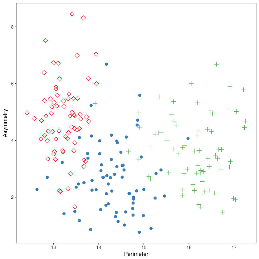
Figure 9: *

(a) True Clustering.

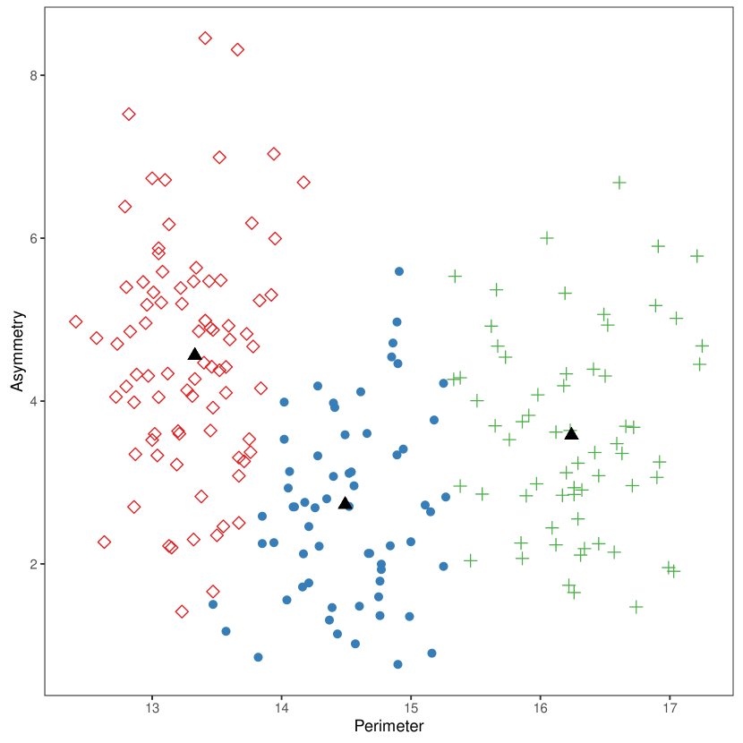
Figure 10: *

(b) Fitted Clustering.

Figure 11: Plots of the true (a) and fitted (b) clusterings of the Seeds dataset, using the GSF-MCP. The lozenges ($\diamond$) indicate the Kama, the blue points ($\bullet$) indicate the Rosa and the green positive symbols ( +) indicate the Canadian seeds. The black triangles ($\blacktriangle$) in the right-hand plot show the means of the fitted Gaussian mixture model by the GSF method using the MCP penalty.

The fitted model by the GSF-MCP, with an upper bound $K=12$, is

$$0.37\leavevmode\nobreak\ {\cal N}\left({{13.33}\choose{4.56}},\widehat{}\bm{\Sigma}\right)+0.31\leavevmode\nobreak\ {\cal N}\left({{14.50}\choose{2.73}},\widehat{}\bm{\Sigma}\right)+0.32\leavevmode\nobreak\ {\cal N}\left({{16.24}\choose{3.58}},\widehat{}\bm{\Sigma}\right)$$

with $\widehat{}\bm{\Sigma}=\begin{pmatrix}0.21&0.04\\ 0.04&1.66\end{pmatrix}$. The log-likelihood value at this estimate is -681.85, and the GSF-MCP correctly classified 88.1% of the data points. The corresponding coefficient plot is reported in Supplement E. We also ran the AIC, BIC and ICL, and they all selected the three-component model

$$0.40\leavevmode\nobreak\ {\cal N}\left({{13.31}\choose{4.52}},\widehat{}\bm{\Sigma}\right)+0.31\leavevmode\nobreak\ {\cal N}\left({{14.55}\choose{2.75}},\widehat{}\bm{\Sigma}\right)+0.29\leavevmode\nobreak\ {\cal N}\left({{16.29}\choose{3.58}},\widehat{}\bm{\Sigma}\right),$$

where $\bm{\Sigma}=\begin{pmatrix}0.20&0.04\\ 0.04&1.70\end{pmatrix}$. The log-likelihood value at this estimate is given by -655.83, and the corresponding classification rate is $87.1\%$.

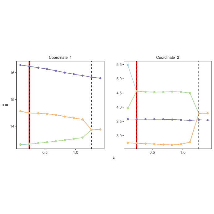
Figure 12: Coefficient plots for the GSF-MCP on the seeds data.

E.7. Regularization plot based on a simulated sample

Figure 13 shows an alternate regularization plot for the simulated sample used in Figures 1 and 2 of the paper.

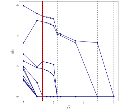
Figure 13: Regularization plot based on the same simulated data as in Figures 1 and 2 of the paper. The estimates $\left\lVert\widehat{\bm{\eta}}_{j}(\lambda)\right\rVert,j=1,\dots,K-1=11$, are plotted against $\lambda$. The red line shows the value $\lambda^{*}$ chosen by the BIC. Since there are four non-zero $\left\lVert\widehat{\bm{\eta}}_{j}(\lambda^{*})\right\rVert$, the fitted model has order $\widehat{K}=5$.

Supplement F: Comparison of the GSF and the Naive GSF

In this section we provide Models F.1 and F.2 cited in Figure 3 of the paper, and we elaborate on the simulation results summarized therein. For both models, $\mathcal{F}$ is chosen to be the family of two-dimensional location-Gaussian densities, with common but unknown covariance, that is

$$p_{G}(\mathbf{y})=\sum_{j=1}^{K}\pi_{j}\frac{1}{\sqrt{(2\pi)^{d}|\bm{\Sigma}}|}\exp\left\{-\frac{1}{2}(\mathbf{y}-\bm{\mu}_{j})^{\top}\bm{\Sigma}^{-1}(\mathbf{y}-\bm{\mu}_{j})\right\},$$

where $\bm{\mu}_{j}\in\mathbb{R}^{d}$, $\pi_{j}\geq 0$, $\sum_{j=1}^{K}\pi_{j}=1$, $j=1,\dots,K$, and we choose $\bm{\Sigma}=\mathbf{I}_{d}$. The true mixing measure $G_{0}=\sum_{j=1}^{K}\pi_{0j}\delta_{\mu_{0j}}$ under Models F.1 and F.2 is respectively given by

$$.5\delta_{(-2,0)}+.5\delta_{(0,1)},\quad\frac{1}{3}\delta_{(1,2)}+\frac{1}{3}\delta_{(1,0)}+\frac{1}{3}\delta_{(-1,-1)}.$$

We implement the Naive GSF for the SCAD penalty using a modification of the EM algorithm with a Local Quadratic Approximation (LQA) of the penalty, as described by Fan and Li, (2001). In this case, the M-Step of the EM algorithm admits a closed-form solution. For fairness of comparison, we also reimplement the GSF using this numerical solution. All other implementation details are analogous to those listed in Section D.2.

We run both the GSF and the Naive GSF on 500 samples of size $n=200$ from Models F.1 and F.2, for the upper bound $K$ ranging from $5$ to $30$ in increments of 5. The simulation results are reported in Table 34.

		GSF						Naive GSF
Model	$\widehat{K}$	5	10	15	20	25	30	5	10	15	20	25	30
F.1	1	.000	.000	.000	.000	.000	.000	.000	.000	.000	.002	.000	.000
	2	.964	.944	.916	.884	.896	.900	.950	.884	.858	.792	.762	.704
	3	.034	.054	.082	.104	.088	.094	.046	.106	.120	.162	.204	.236
	4	.002	.002	.002	.012	.016	.006	.004	.010	.020	.040	.030	.050
	5	.000	.000	.000	.000	.000	.000	.000	.000	.002	.004	.002	.010
	6	.000	.000	.000	.000	.000	.000	.000	.000	.000	.000	.002	.000
F.2	2	.274	.276	.264	.286	.274	.304	.242	.274	.288	.296	.318	.294
	3	.690	.684	.688	.656	.664	.630	.714	.656	.616	.594	.524	.538
	4	.036	.040	.048	.052	.060	.066	.044	.066	.092	.106	.144	.144
	5	.000	.000	.000	.006	.002	.000	.000	.004	.002	.000	.010	.020
	6	.000	.000	.000	.000	.000	.000	.000	.000	.002	.004	.004	.004

Table 34: Results of the simulation studies, for $K$ ranging from 5 to 30.

References

- Akaike, (1974) Akaike, H. (1974). A new look at the statistical model identification. IEEE Trans. Autom. Control, AC-19:716–723.
- Bechtel et al., (1993) Bechtel, Y. C., Bonaiti-Pellie, C., Poisson, N., Magnette, J., and Bechtel, P. R. (1993). A population and family study of n-acetyltransferase using caffeine urinary metabolites. Clin. Pharmacol. Ther., 54:134–141.
- Benaglia et al., (2009) Benaglia, T., Chauveau, D., Hunter, D., and Young, D. (2009). mixtools: An r package for analyzing finite mixture models. J. Stat. Softw., 32:1–29.
- Biernacki et al., (2000) Biernacki, C., Celeux, G., and Govaert, G. (2000). Assessing a mixture model for clustering with the integrated completed likelihood. IEEE Trans. Pattern. Anal. Mach. Intell., 22:719–725.
- Bosch-Domènech et al., (2010) Bosch-Domènech, A., Montalvo, J. G., Nagel, R., and Satorra, A. (2010). A finite mixture analysis of beauty-contest data using generalized beta distributions. Exp. Econm., 13:461–475.
- Breheny and Huang, (2015) Breheny, P. and Huang, J. (2015). Group descent algorithms for nonconvex penalized linear and logistic regression models with grouped predictors. Statist. Comput., 25:173–187.
- Charytanowicz et al., (2010) Charytanowicz, M., Niewczas, J., Kulczycki, P., Kowalski, P. A., Łukasik, S., and Zak, S. (2010). Complete gradient clustering algorithm for features analysis of x-ray images. Adv. Intell. Sof. Comput., 69:15–24.
- Chen and Chen, (2003) Chen, H. and Chen, J. (2003). Tests for homogeneity in normal mixtures in the presence of a structural parameter. Statist. Sinica, 13:351–365.
- Chen et al., (2004) Chen, H., Chen, J., and Kalbfleisch, J. (2004). Testing for a finite mixture model with two components. J. R. Stat. Soc. Ser. B. Stat. Methodol., 66:95–115.
- Chen, (1995) Chen, J. (1995). Optimal rate of convergence for finite mixture models. Ann. Statist., 23:221–233.
- Chen and Kalbfleisch, (1996) Chen, J. and Kalbfleisch, J. (1996). Penalized minimum-distance estimates in finite mixture models. Canad. J. Statist., 24:167–175.
- Chen and Khalili, (2008) Chen, J. and Khalili, A. (2008). Order selection in finite mixture models with a nonsmooth penalty. J. Amer. Statist. Assoc., 103:1674–1683.
- Chen and Li, (2009) Chen, J. and Li, P. (2009). Hypothesis test for normal mixture models: The em approach. Ann. Statist., 37:2523–2542.
- Dacunha-Castelle et al., (1999) Dacunha-Castelle, D., Gassiat, E., et al. (1999). Testing the order of a model using locally conic parametrization: population mixtures and stationary arma processes. Ann. Statist., 27:1178–1209.
- Dempster et al., (1977) Dempster, A. P., Laird, N. M., and Rubin, D. B. (1977). Maximum likelihood from incomplete data via the em algorithm. J. R. Stat. Soc. Ser. B. Stat. Methodol., 39:1–38.
- Donoho and Johnstone, (1994) Donoho, D. L. and Johnstone, J. M. (1994). Ideal spatial adaptation by wavelet shrinkage. Biometrika, 81:425–455.
- Drton and Plummer, (2017) Drton, M. and Plummer, M. (2017). A bayesian information criterion for singular models. J. R. Stat. Soc. Ser. B. Stat. Methodol., 79(2):323–380.
- Fan and Li, (2001) Fan, J. and Li, R. (2001). Variable selection via nonconcave penalized likelihood and its oracle properties. J. Amer. Statist. Assoc., 96:1348–1360.
- Fan et al., (2018) Fan, J., Liu, H., Sun, Q., Zhang, T., et al. (2018). I-lamm for sparse learning: Simultaneous control of algorithmic complexity and statistical error. Ann. Statist., 46:814–841.
- Fraley and Raftery, (1999) Fraley, C. and Raftery, A. E. (1999). Mclust: Software for model-based cluster analysis. J. Classification, 16:297–306.
- Friedman et al., (2008) Friedman, J., Hastie, T., and Tibshirani, R. (2008). The elements of statistical learning: data mining, inference, and prediction. Springer Series in Statistics New York, 2 edition.
- Frühwirth-Schnatter, (2006) Frühwirth-Schnatter, S. (2006). Finite mixture and Markov switching models. Springer, Berlin, 1st edition.
- Genovese et al., (2000) Genovese, C. R., Wasserman, L., et al. (2000). Rates of convergence for the gaussian mixture sieve. Ann. Statist., 28:1105–1127.
- Ghosal and van der Vaart, (2001) Ghosal, S. and van der Vaart, A. W. (2001). Entropies and rates of convergence for maximum likelihood and bayes estimation for mixtures of normal densities. Ann. Statist., 29:1233–1263.
- Goodfellow et al., (2016) Goodfellow, I., Bengio, Y., Courville, A., and Bengio, Y. (2016). Deep learning, volume 1. MIT press Cambridge.
- Grenier, (2016) Grenier, I. (2016). Bayesian model selection for deep exponential families. unpublished thesis.
- Guha et al., (2019) Guha, A., Ho, N., and Nguyen, X. (2019). On posterior contraction of parameters and interpretability in Bayesian mixture modeling. arXiv preprint arXiv:1901.05078.
- Hathaway, (1986) Hathaway, R. J. (1986). A constrained em algorithm for univariate normal mixtures. J. Stat. Comput. Simul., 23:211–230.
- Heinrich and Kahn, (2018) Heinrich, P. and Kahn, J. (2018). Strong identifiability and optimal minimax rates for finite mixture estimation. Ann. Statist., 46:2844–2870.
- Ho, (2017) Ho, N. (2017). Parameter estimation and multilevel clustering with mixture and hierarchical models. PhD thesis, University of Michigan, Ann Arbor.
- Ho and Nguyen, (2016) Ho, N. and Nguyen, X. (2016). Singularity structures and impacts on parameter estimation in finite mixtures of distributions. arXiv preprint arXiv:1609.02655.
- (32) Ho, N., Nguyen, X., et al. (2016a). Convergence rates of parameter estimation for some weakly identifiable finite mixtures. Ann. Statist., 44:2726–2755.
- (33) Ho, N., Nguyen, X., et al. (2016b). On strong identifiability and convergence rates of parameter estimation in finite mixtures. Electron. J. Stat., 10:271–307.
- Ho et al., (2017) Ho, N., Nguyen, X., and Ritov, Y. (2017). Robust estimation of mixing measures in finite mixture models. arXiv preprint arXiv:1709.08094.
- Ho et al., (2019) Ho, N., Yang, C.-Y., and Jordan, M. I. (2019). Convergence rates for gaussian mixtures of experts. arXiv preprint arXiv:1907.04377.
- Holzmann et al., (2004) Holzmann, H., Munk, A., and Stratmann, B. (2004). Identifiability of finite mixtures-with applications to circular distributions. Sankhya A, 69:440–449.
- Hung et al., (2013) Hung, Y., Wang, Y., Zarnitsyna, V., Zhu, C., and Wu, C. F. J. (2013). Hidden markov models with applications in cell adhesion experiments. J. Amer. Statist. Assoc., 108:1469–1479.
- Ishwaran et al., (2001) Ishwaran, H., James, L. F., and Sun, J. (2001). Bayesian model selection in finite mixtures by marginal density decompositions. J. Amer. Statist. Assoc., 96:1316–1332.
- James et al., (2001) James, L. F., Priebe, C. E., and Marchette, D. J. (2001). Consistent estimation of mixture complexity. Ann. Statist., 29:1281–1296.
- Kalman, (1984) Kalman, D. (1984). The generalized vandermonde matrix. Mathematics Magazine, 57(1):15–21.
- Keribin, (2000) Keribin, C. (2000). Consistent estimation of the order of mixture models. Sankhya A, 62:49–66.
- Lee and McLachlan, (2013) Lee, S. X. and McLachlan, G. J. (2013). Model-based clustering and classification with non-normal mixture distributions. Stat. Method Appl., 22:427–454.
- Leroux, (1992) Leroux, B. G. (1992). Consistent estimation of a mixing distribution. Ann. Statist., 20:1350–1360.
- Li and Chen, (2010) Li, P. and Chen, J. (2010). Testing the order of a finite mixture. J. Amer. Statist. Assoc., 105(491):1084–1092.
- Li et al., (2009) Li, P., Chen, J., and Marriott, P. (2009). Non-finite fisher information and homogeneity: an em approach. Biometrika, 96(2):411–426.
- Liu and Shao, (2003) Liu, X. and Shao, Y. (2003). Asymptotics for likelihood ratio tests under loss of identifiability. Ann. Statist., 31:807–832.
- McLachlan and Peel, (2000) McLachlan, G. and Peel, D. (2000). Finite mixture models. John Wiley & Sons.
- McLachlan, (1987) McLachlan, G. J. (1987). On bootstrapping the likelihood ratio test stastistic for the number of components in a normal mixture. J. R. Stat. Soc. Ser. C. Appl. Stat., 36:318–324.
- Miller and Harrison, (2018) Miller, J. W. and Harrison, M. T. (2018). Mixture models with a prior on the number of components. J. Amer. Statist. Assoc., 113(521):340–356.
- Morel and Nagaraj, (1993) Morel, J. G. and Nagaraj, N. K. (1993). A finite mixture distribution for modelling multinomial extra variation. Biometrika, 80(2):363–371.
- Morris et al., (1996) Morris, T. H., Richmond, D. R., and Grimshaw, S. D. (1996). Orientation of dinosaur bones in riverine environments: Insights into sedimentary dynamics and taphonomy. The Continental Jurassic: Museum of Northern Arizona, Flagstaff, pages 521–530.
- Mosimann, (1962) Mosimann, J. E. (1962). On the compound multinomial distribution, the multivariate -distribution, and correlations among proportions. Biometrika, 49(1/2):65–82.
- Nesterov, (2004) Nesterov, Y. (2004). Introductory Lectures on Convex Optimization. Kluwer Academic Publishers, New York.
- Nguyen, (2013) Nguyen, X. (2013). Convergence of latent mixing measures in finite and infinite mixture models. Ann. Statist., 41(1):370–400.
- Nobile, (1994) Nobile, A. (1994). Bayesian Analysis of Finite Mixture Distributions. PhD Thesis, PhD Thesis. Carnegie Mellon University, Pittsburgh.
- Petralia et al., (2012) Petralia, F., Rao, V., and Dunson, D. (2012). Repulsive mixtures. In Pereira, F., Burges, C. J. C., Bottou, L., and Weinberger, K. Q., editors, Advances in Neural Information Processing Systems, volume 25, pages 1889–1897. Curran Associates, Inc.
- Richardson and Green, (1997) Richardson, S. and Green, P. J. (1997). On bayesian analysis of mixtures with an unknown number of components (with discussion). J. R. Stat. Soc. Ser. B. Stat. Methodol., 59:731–792.
- Rousseau and Mengersen, (2011) Rousseau, J. and Mengersen, K. (2011). Asymptotic behaviour of the posterior distribution in overfitted mixture models. J. R. Stat. Soc. Ser. B. Stat. Methodol., 73:689–710.
- Schwarz, (1978) Schwarz, G. (1978). Estimating the dimension of a model. Ann. Statist., 6:461–464.
- Serfling, (2002) Serfling, R. J. (2002). Approximation theorems of mathematical statistics. John Wiley & Sons.
- Stephens, (2000) Stephens, M. (2000). Bayesian analysis of mixture models with an unknown number of components-an alternative to reversible jump methods. Ann. Statist., 28:40–74.
- Teicher, (1963) Teicher, H. (1963). Identifiability of finite mixtures. Ann. Math. Stat, 34:1265–1269.
- Thompson et al., (1998) Thompson, T. J., Smith, P. J., and Boyle, J. P. (1998). Finite mixture models with concomitant information: assessing diagnostic criteria for diabetes. J. R. Stat. Soc. Ser. C. Appl. Stat., 47:393–404.
- van de Geer, (2000) van de Geer, S. (2000). Empirical Processes in M-estimation. Cambridge university press.
- Villani, (2003) Villani, C. (2003). Topics in optimal transportation. Number 58. American Mathematical Soc.
- Wong et al., (1995) Wong, W. H., Shen, X., et al. (1995). Probability inequalities for likelihood ratios and convergence rates of sieve mles. Ann. Statist., 23:339–362.
- Woo and Sriram, (2006) Woo, M.-J. and Sriram, T. (2006). Robust estimation of mixture complexity. J. Amer. Statist. Assoc., 101:1475–1486.
- Wu et al., (2020) Wu, Y., Yang, P., et al. (2020). Optimal estimation of gaussian mixtures via denoised method of moments. Annals of Statistics, 48(4):1981–2007.
- Xie and Xu, (2020) Xie, F. and Xu, Y. (2020). Bayesian Repulsive Gaussian Mixture Model. Journal of the American Statistical Association, 115(529):187–203.
- Xu and Chen, (2015) Xu, C. and Chen, J. (2015). A thresholding algorithm for order selection in finite mixture models. Commun. Stat. - Simul. Comput, 44:433–453.
- (71) Zhang, C.-H. et al. (2010a). Nearly unbiased variable selection under minimax concave penalty. Ann. Statist., 38:894–942.
- (72) Zhang, Y., Li, R., and Tsai, C.-L. (2010b). Regularization parameter pelections via generalized information criterion. J. Amer. Statist. Assoc., 105:312–323.
- Zhao et al., (2015) Zhao, J., Jin, L., and Shi, L. (2015). Mixture model selection via hierarchical bic. Comput. Statist. Data Anal., 88:139–153.
- Zou, (2006) Zou, H. (2006). The adaptive lasso and its oracle properties. J. Amer. Statist. Assoc., 101:1418–1429.
- Zou and Li, (2008) Zou, H. and Li, R. (2008). One-step sparse estimates in nonconcave penalized likelihood models. Ann. Statist., 36:1509—1533.