Supplemental Material: Self-organization and chiral self-sorting of active semiflexible filaments with intrinsic curvature

I Simulation model

We model our filaments as discretized wormlike chains kratky49 with inextensible segments of length $a$. We have adopted the algorithm by Montesi et. al montesi05 for the constrained Brownian dynamics of bead-rod wormlike chains with anisotropic friction. The implementation of the algorithm in our simulations has been covered in previous work moore20 ; moore20a . What follows here is an overview of the algorithm, as well as the details on our implementation of intrinsic curvature and activity.

Filaments are represented by $N$ sites and $N-1$ segments, with fixed segment length $a$, contour length $L=(N-1)a$, and anisotropic friction, $\zeta_{\bot}=2\zeta_{\parallel}$. The position of each site $\mathbf{r}_{i}$ is updated using a midstep algorithm

$$\mathbf{r}_{i}^{(1/2)} =\mathbf{r}_{i}^{(0)}+\frac{\Delta t}{2}\mathbf{v}_{i}^{(0)},$$ (1)

$$\mathbf{r}_{i}^{(1)} =\mathbf{r}_{i}^{(0)}+\Delta t\ \mathbf{v}_{i}^{(1/2)},$$

where $\Delta t$ is the time step, $\mathbf{v}_{i}^{(0)}$ is the initial velocity of site $i$ at the initial position $\mathbf{r}_{i}^{(0)}$, and $\mathbf{v}_{i}^{(1/2)}$ is the velocity of site $i$ recalculated at the midstep position $\mathbf{r}_{i}^{(1/2)}$ with the stochastic forces that were calculated at $\mathbf{r}_{i}^{(0)}$. The position $\mathbf{r}_{i}^{(1)}$ is referred to as the fullstep position.

Each site $i$ is assigned an orientation, corresponding to the orientation of the segment attaching it to site $i+1$,

$$\mathbf{u}_{i}=\frac{\mathbf{r}_{i+1}-\mathbf{r}_{i}}{|\mathbf{r}_{i+1}-\mathbf{r}_{i}|}=\frac{1}{a}(\mathbf{r}_{i+1}-\mathbf{r}_{i}).$$ (2)

The orientation of the last site of the filament is set equal to that of its only neighboring segment, so that $\mathbf{u}_{N}=\mathbf{u}_{N-1}$.

The velocity of each site is

$$\mathbf{v}_{i}=\bm{\zeta}^{-1}_{i}\cdot\mathbf{F}^{\text{tot}}_{i},$$ (3)

where $\bm{\zeta}^{-1}_{i}$ is an anisotropic friction tensor,

$$\bm{\zeta}^{-1}_{i} =\frac{1}{\zeta_{\parallel}^{i}}\tilde{\mathbf{u}}_{i}\otimes\tilde{\mathbf{u}}_{i}+\frac{1}{\zeta_{\bot}^{i}}\big{(}\mathbf{I}-\tilde{\mathbf{u}}_{i}\otimes\tilde{\mathbf{u}}_{i}\big{)}.$$ (4)

and $\tilde{\mathbf{u}}_{i}$ is the vector tangent to site $i$, which is the average of the orientations $\mathbf{u}_{i}$ of its neighboring segments,

$$\tilde{\mathbf{u}}_{i}=\frac{(\mathbf{u}_{i}+\mathbf{u}_{i-1})}{|\mathbf{u}_{i}+\mathbf{u}_{i-1}|}$$ (5)

for $2\leq i\leq N$, and $\tilde{\mathbf{u}}_{1}=\mathbf{u}_{1}$, $\tilde{\mathbf{u}}_{N}=\mathbf{u}_{N-1}$ at the chain ends.

In the absence of filament interactions and driving, the total force on site $i$ is the sum

$$\mathbf{F}^{\text{tot}}_{i}=\mathbf{F}_{i}^{\text{bend}}+\mathbf{F}_{i}^{\text{tension}}+\mathbf{F}_{i}^{\text{rand}},$$ (6)

which include bending forces, tension forces, and random forces. The random forces are due to thermal contact with a heat bath at temperature $T$, with the properties $\langle F_{\text{rand}}\rangle=0$ and $\langle F^{2}_{\text{rand}}\rangle=2\zeta k_{B}T$ to obey the fluctuation dissipation theorem. The random forces are projected onto the chain such that the forces do not conflict with the constraints due to the fixed segment length, and are described in detail by Montesi et al. montesi05 .

The diffusivity of a rigid filament is $D=k_{B}T/\zeta=k_{B}T/N\zeta_{i}$, where $\zeta_{i}$ is the local friction acting on site $i$. The friction depends on the filament aspect ratio $L/\sigma$, where $\sigma$ is the diameter of the chain. In the regime of rigid, infinitely thin rods, the coefficient of friction is given by doi88 ,

$$\lim_{L/\sigma\to\infty}\zeta_{\bot}=4\pi\eta_{s}L\epsilon.$$ (7)

where $\eta_{s}$ is the fluid viscosity. Each site experiences a local friction given by

$$\zeta_{\bot}^{\text{i}}=4\pi\eta_{s}a\epsilon f(\epsilon).$$ (8)

where $\epsilon=1/\ln{(L/\sigma)}$ and

$$f(\epsilon)=\frac{1+0.64\epsilon}{1-1.15\epsilon}+1.659\epsilon^{2}.$$ (9)

is the geometric correction factor for finite aspect ratio filaments.

The bending energy of a discrete wormlike chain for $N\gg 1$ is approximated by

$$U_{\text{bend}}=-\frac{\kappa}{a}\sum_{k=2}^{N-1}\mathbf{u}_{k}\cdot\mathbf{u}_{k-1},$$ (10)

where $\kappa$ is the bending rigidity, which is related to the persistence length $L_{p}$ of the wormlike chain as $\kappa=L_{p}k_{B}T$. Note that we are adopting the convention that the previous equation is true in all dimensions $d$ of wormlike chains, unlike the convention adopted by Landau and Lifshitz where $\kappa/k_{B}T=(d-1)L_{p}/2$ landau86 . Our convention results in a Kuhn length that depends on dimensionality, $b=(d-1)L_{p}$.

The bending force is $\mathbf{F}^{\text{bend}}_{i}=-\partial U_{\text{bend}}/\partial\mathbf{r}_{i}$. The implementation of the bending forces coincides with metric forces, which come from a metric pseudo-potential that is necessary for the filament conformation to have the expected statistical behavior in the flexible limit, $L_{p}\ll L$.

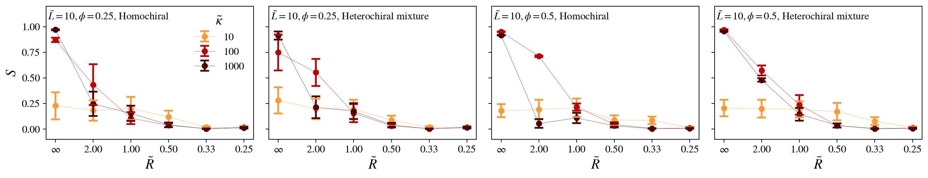
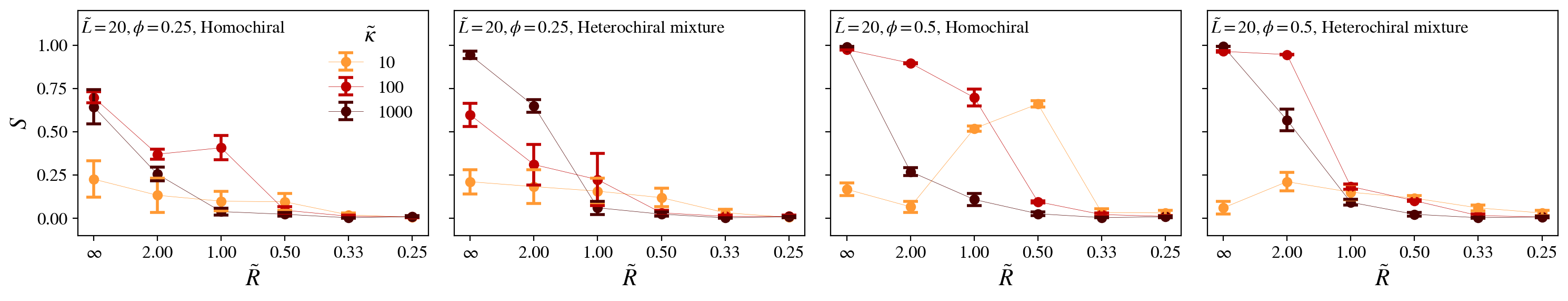
Figure 1: Values of the global nematic order $S$ plotted as a function of $\tilde{R}$ for all simulation parameters. Top row plots are for filaments with aspect ratio $\tilde{L}=10$ and the bottom row $\tilde{L}=20$.

The bending forces are calculated to include metric forces resulting from a geometric pseudo-potential fixman78 ; montesi05 . The metric pseudo-potential is necessary to observe the proper equilibrium behavior of discrete wormlike chains with low persistence lengths. In the work of Pasquali et. al pasquali02 , it was shown that the bending and metric forces together are

$$\mathbf{F}_{i}^{\text{bend}}+\mathbf{F}_{i}^{\text{metric}}=\frac{1}{a}\sum_{k=2}^{N-1}\kappa_{k}^{\text{eff}}\frac{\partial(\mathbf{u}_{k}\cdot\mathbf{u}_{k-1})}{\partial\mathbf{r}_{i}},$$ (11)

where $\kappa^{\text{eff}}$ is an effective bending rigidity with a conformational dependence,

$$\kappa_{i}^{\text{eff}}=\kappa+k_{B}Ta\hat{G}^{-1}_{i-1,i},$$ (12)

where $\hat{G}$ is the metric tensor pasquali02 ; montesi05 . The derivative in Eqn. 11 can be expanded so that the equation as implemented in our simulation is

$$\mathbf{F}_{i}^{\text{bend}}+\mathbf{F}_{i}^{\text{metric}}=\frac{1}{a^{2}}\sum_{k=2}^{N-1}\kappa_{k}^{\text{eff}}\Big{(}(\delta_{i,k+1}-\delta_{i,k})(\mathbf{I}-\mathbf{u}_{k}\otimes\mathbf{u}_{k})\mathbf{u}_{k-1}+(\delta_{i,k}-\delta_{i,k-1})(\mathbf{I}-\mathbf{u}_{k-1}\otimes\mathbf{u}_{k-1})\mathbf{u}_{k}\Big{)}.$$ (13)

An intrinsic curvature was added to the filament model by modifying the bending potential in Eqn. 10 to have an offset angle $\phi_{0}$,

$$U_{\text{bend}}=-\frac{\kappa}{a}\sum_{k=2}^{N-1}\cos{(\theta_{k,k-1}-\phi_{0})},$$ (14)

where $\theta_{k,k-1}=\arccos{(\mathbf{u}_{k}\cdot\mathbf{u}_{k-1})}$ is the angle between site orientations $k$ and $k-1$, and $\phi_{0}=ad\phi/ds$ corresponds to the expected angle between two segments of length $a$ with a curvature per unit length $d\phi/ds$.

It can be shown that the term in the sum of Eqn. 14 can be rewritten as

$$\cos{(\theta_{k,k-1}-\phi_{0})}=\mathbf{R}\mathbf{u}_{k}\cdot\mathbf{R}^{-1}\mathbf{u}_{k-1},$$ (15)

where $\mathbf{R}$ is a rotation matrix that rotates the orientation vector $\mathbf{u}_{k}$ by an angle $\phi_{0}/2$,

$$\mathbf{R}=\begin{pmatrix}\cos(\phi_{0}/2)&-\sin(\phi_{0}/2)\\ \sin(\phi_{0}/2)&\cos(\phi_{0}/2)\end{pmatrix},$$ (16)

and its inverse $\mathbf{R}^{-1}$ rotates the orientation vector $\mathbf{u}_{k-1}$ by an angle $-\phi_{0}/2$. The combined bending and metric forces from Eqn. 11 with intrinsic curvature are therefore

$$\mathbf{F}_{i}^{\text{bend}}+\mathbf{F}_{i}^{\text{metric}}=\frac{1}{a}\sum_{k=2}^{N-1}\kappa_{k}^{\text{eff}}\frac{\partial(\mathbf{R}\mathbf{u}_{k}\cdot\mathbf{R}^{-1}\mathbf{u}_{k-1})}{\partial\mathbf{r}_{i}},$$ (17)

which can be expanded in the same way as Eqn. 13.

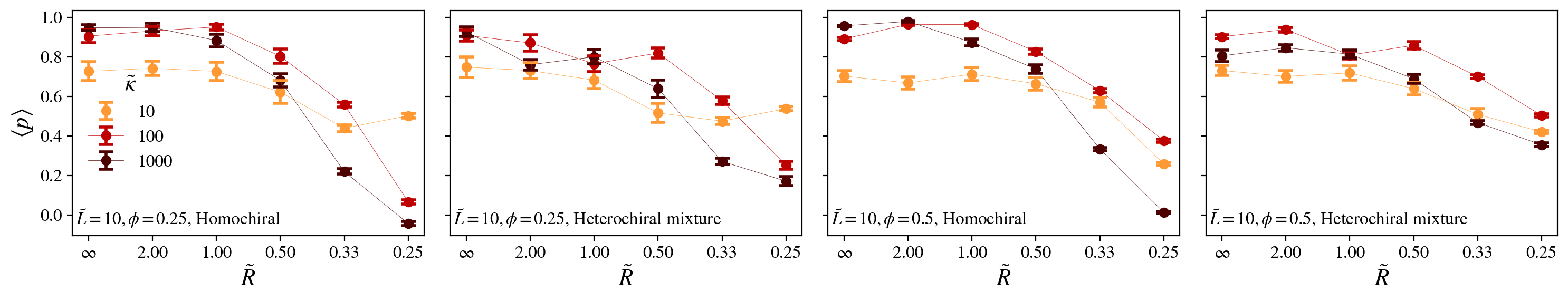
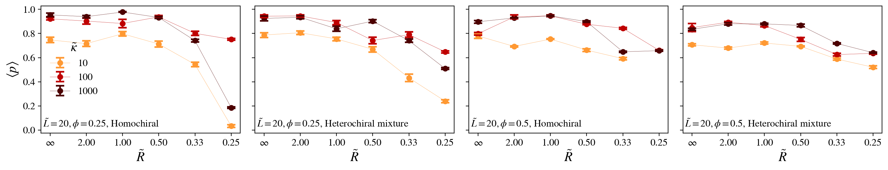
Figure 2: Values of the average local polar order $\langle p\rangle$ of simulations plotted as a function of $\tilde{R}$ for all simulation parameters. Top row plots are for filaments with aspect ratio $\tilde{L}=10$ and the bottom row $\tilde{L}=20$.

Filament driving forces are modeled as a uniform linear force density $f_{\text{dr}}$ that is directed along the local filament segment orientations,

$$\mathbf{F}_{\text{dr}}=f_{\text{dr}}\mathbf{u}_{i}.$$ (18)

The assumptions of this model match observations of experiments with gliding filaments driven by a lattice of motor proteins, which found that that filament velocities were constant, despite the persistent binding and unbinding of motors liu11 .

II Model implementation

Simulation software for the filament model is written in C++ and the source code is publicly available online  moore20 . The software is also available as a pre-installed binary on Singularity and Docker images. The simulations were run on the Summit computing cluster anderson17 and parallelized using OpenMP.

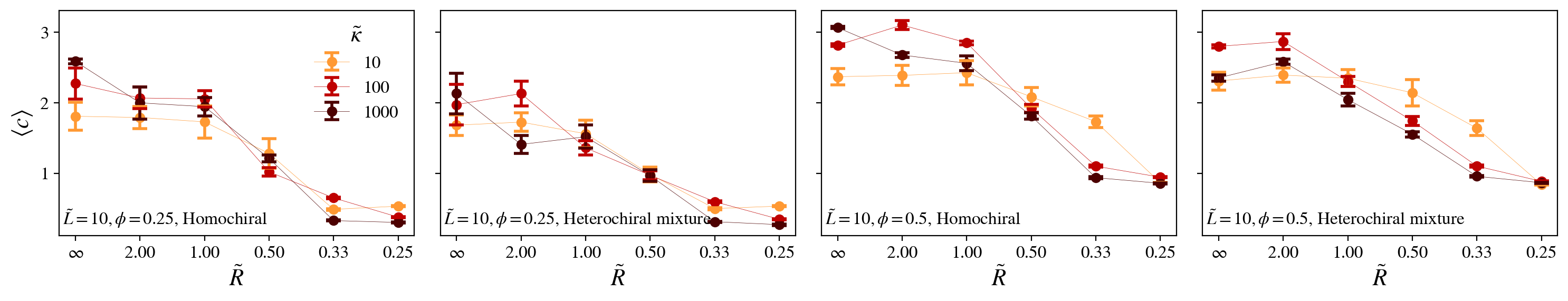
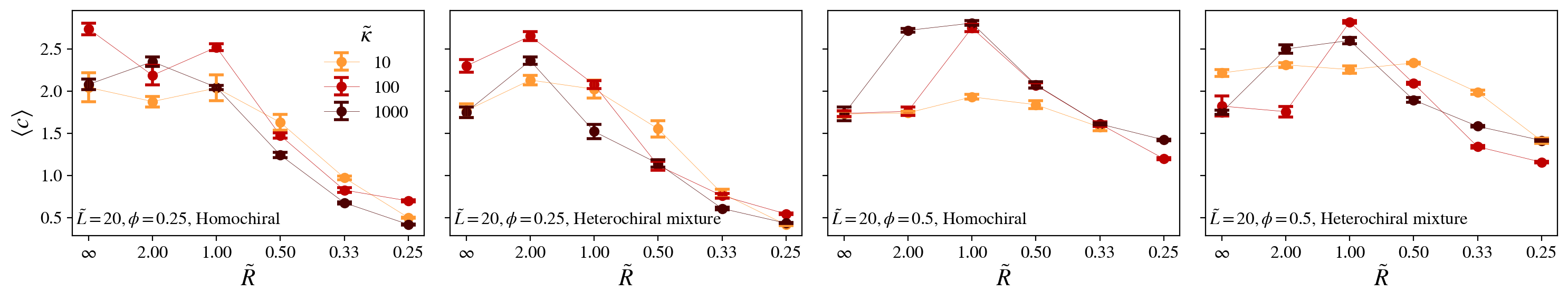
Figure 3: Values of the average contact number $\langle c\rangle$ plotted as a function of $\tilde{R}$ for all simulation parameters. Top row plots are for filaments with aspect ratio $\tilde{L}=10$ and the bottom row $\tilde{L}=20$.

III Simulation parameters

Important parameters of our simulation are the filament contour length $L$, diameter $\sigma$, bending rigidity $\kappa$, driving force per unit length $f_{dr}$, filament radius of curvature $R$, simulation box diameter $L_{sys}$, and filament density $\phi$. Our simulations have filament aspect ratios $\tilde{L}=L/\sigma=10$ and $20$, and the system size is $~{}\tilde{L}_{sys}=L_{sys}/L=10$. In our dimensionless reduced units, $\sigma$, $k_{B}T$, and $D$ are set to be unity, where $D$ is the diffusion coefficient for a sphere of diameter $\sigma$, such that the viscosity is $1/3\pi$. The driving force in reduced units is $f_{dr}=15$, such that the Péclet number is $\text{Pe}=f_{dr}L^{2}/k_{B}T\approx 5\times 10^{4}$, which was chosen to avoid issues arising from the effects of filament softening due to tangential driving isele-holder15 ; anand18 ; gupta19 ; peterson20 ; moore20a .

The dimensionless parameters used in our analysis are $\tilde{\kappa}=\kappa/Lk_{B}T=L_{p}/L$, where $L_{p}$ is the filament persistence length, the filament radius of curvature $\tilde{R}=R/L$, and filament density in terms of the particle packing fraction $\phi=A_{\text{fil}}/A_{\text{sys}}$, where $A_{\text{sys}}$ is the area of the 2D periodic simulation space and $A_{\text{fil}}=N(L\sigma+\pi\sigma^{2})$ is the area occupied by $N$ 2D spherocylindrical filaments.

We used a dynamic timestep in the half-step integration algorithm, with a maximum timestep $\Delta t=2.5\times 10^{-5}\tau$, where $\tau$ is the average time for a sphere of diameter $\sigma$ to diffuse its own diameter. If ever forces between any two particles ever exceed a preset threshold of $10^{6}$ reduced force units, all particles are returned to the previous full-step positions, the timestep is reduced by a factor of 2, and forces are recalculated. The time resolution of filament positions for the purposes of analysis are fixed to be $\Delta t_{\text{max}}$. The active timescale used in our analysis is the time required for a straight filament to glide its own length $\tau_{A}=l/v_{dr}=1/\zeta_{\parallel}f_{dr}$, which is $0.66\tau$ for $\text{Pe}=5\times 10^{4}$.

Filaments in the simulation were initialized by randomly inserting straight filaments parallel to one axis of the simulation box in a nematic arrangement, allowing the filaments to relax and diffuse without activity for $100\tau$ before introducing driving forces. Simulations terminated once they were determined to have reached a steady state, when order parameters appeared to converge to constant values.

IV Flocking analysis

Long-range structural order in our simulations filaments is captured by the nematic order parameter of the system $S$, which is the largest eigenvalue of the 2D nematic order tensor

$$\mathbf{Q}=\frac{1}{N}\sum_{i=1}^{N}(2\mathbf{u}_{i}\otimes\mathbf{u}_{i}-\mathbf{I}),$$ (19)

where $\mathbf{I}$ is the unit tensor. High nematic order indicates that flocks have aggregated into giant flocks, which tend to dominate the overall system structure. Nematic order is present for rigid filaments and large radius of curvature (Fig. 1).

Although curvature and flexibility inhibit long-range order, polar flocks are present at all but the highest curvatures examined here, $\tilde{R}=0.25$. Following previous work, flocking behavior was identified by measuring the filament contact number $c_{i}\sum_{i\neq j}=e^{-(r_{ij}/\sigma)^{2}}$ and the local polar order parameter $p_{i}=\sum_{i\neq j}\mathbf{u}_{i}\cdot\mathbf{u}_{j}e^{-(r_{ij}/\sigma)^{2}}/c_{i}$, with sums ranging over all filament segments, excluding intrafilament segments. The time and ensemble-average of the local polar order all simulation parameters is plotted in Fig. 2.

Systems with polar-ordered collective motion exhibit giant number fluctuations (GNF) gregoire04 ; chate08 ; ginelli10 ; ginelli16 . Number fluctuations are derived from the mean $\langle N\rangle$ and standard deviation $\Delta N$ of the particle number within a subregion of the system. Varying the size of the region leads to a power-law scaling behavior $\Delta N\propto\langle N\rangle^{\alpha}$. For equilibrium systems, number fluctuations scale with the exponent $\alpha=1/2$, whereas systems with GNF exhibit scaling with $\alpha>0.5$, with the Vicsek model having $\alpha\approx 0.8$ chate08 ; ginelli10 .

The number fluctuation scaling for all simulations is plotted in Fig. 5. In the flocking regime with straight filaments, filaments exhibit GNF with $\alpha\approx 0.8$. The number fluctuations decrease with increasing filament curvature, and in some cases enters a regime with $\alpha<0.5$ indicating subdiffusive behavior, causing small density fluctuations at short timescales.

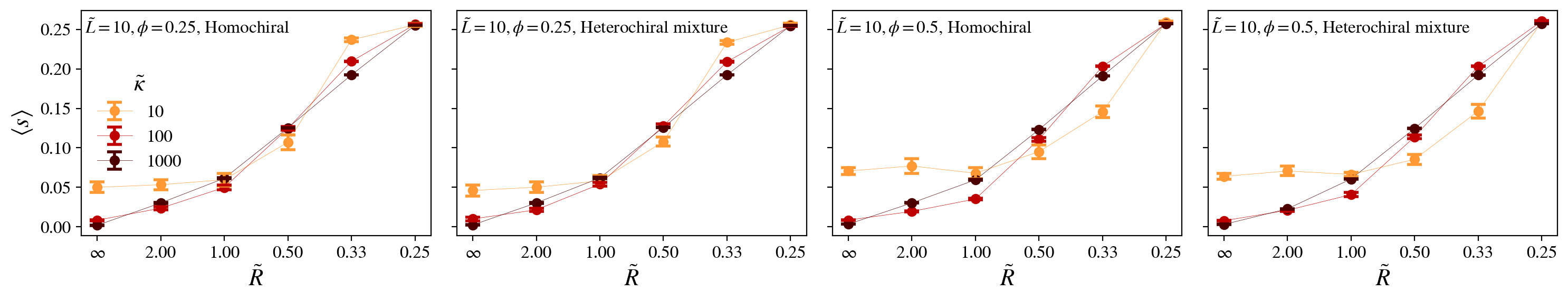
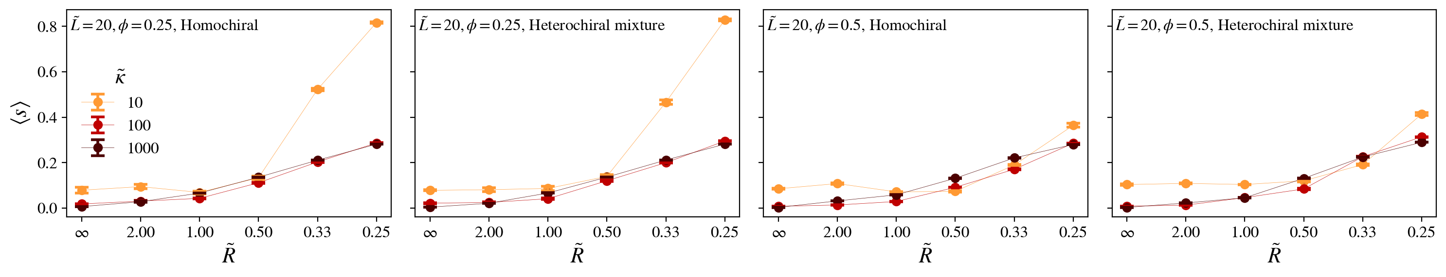
Figure 4: Values of the average spiral number $\langle s\rangle$ plotted as a function of $\tilde{R}$ for all simulation parameters. Top row plots are for filaments with aspect ratio $\tilde{L}=10$ and the bottom row $\tilde{L}=20$.

For a driven flexible filament, there is a chance for the filament to self-interact and wrap upon itself, winding into a spiral-like structure. We have previously measured the spiral-similarity of bent filaments using a spiral number $\langle s\rangle$ moore20a . The spiral number for an individual filament is calculated by measuring the angle $\theta_{i}$ swept by traversing its contour length from tail to head originating from the center of curvature of the filament, $s_{i}=\frac{1}{2\pi}\theta_{i}$. A straight filament will have a spiral number $s_{i}=0$, a filament bent into a perfect circle has $s_{i}=1$, and filaments that form tightly-wound spirals may have a spiral number $s_{i}>1$.

The average spiral number for curved filaments at equilibrium will reflect the radius of curvature of the filament. However, effects due to interactions, driving, and flexibility will modify the overall spiral number. We find that flexible filaments with aspect ratio $\tilde{L}=10$ have higher spiral numbers than more rigid filaments at large $\tilde{R}$. However, we surprisingly find that flexible filaments with intermediate $\tilde{R}$ have a slightly smaller spiral number than the most rigid filaments in our simulations (Fig. 4). This is likely due to the flexible filaments forming heterochiral flocks, while rigid filaments only form homochiral clusters. For filaments with aspect ratio $\tilde{L}=20$, filaments have a much higher spiral number compared to other rigidities when filaments have small radius of curvature, $\tilde{R}=0.25$, indicating the formation of tightly-wound and dynamically frozen spirals. The formation of these structures is likely the cause of the subdiffusive behavior for flexible filaments even at long times.

V Mean-squared displacement

The mean-squared displacements (MSD) of filaments for both inactive and active filaments were calculated using the equation $\langle\big{(}\mathbf{r}(t)-\mathbf{r}(t_{0})\big{)}^{2}\rangle$, where the brackets $\langle...\rangle$ denote an average over the ensemble of filaments and time averages for different values of $t_{0}$ separated by a minimum of $10\tau_{A}$. Example MSDs for $\tilde{L}=10$ are plotted in Fig. 6 on a log-log scale, with the gray dashed line denoting linear time-scaling behavior.

The effective diffusion coefficient for active filaments $D_{\text{active}}$ was calculated using the final $25\tau_{A}$ interval of the MSD to limit analysis to long-time transport behavior of filaments, assuming a linear time scaling. To determine whether the long-time behavior was diffusive, we calculated the power-law scaling of the effective diffusion coefficient with respect to time, $\langle\big{(}\mathbf{r}(t)-\mathbf{r}(t_{0})\big{)}^{2}\rangle\propto Dt^{\alpha}$ by measuring the slope of the log-log transform of the MSD using a weighted least squares linear regression model, with weights derived from the standard error of the mean for values of the MSD.

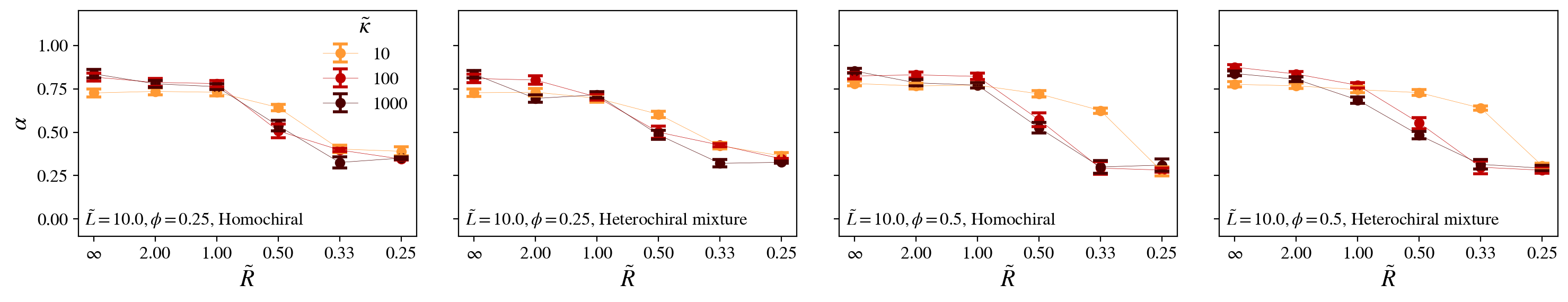
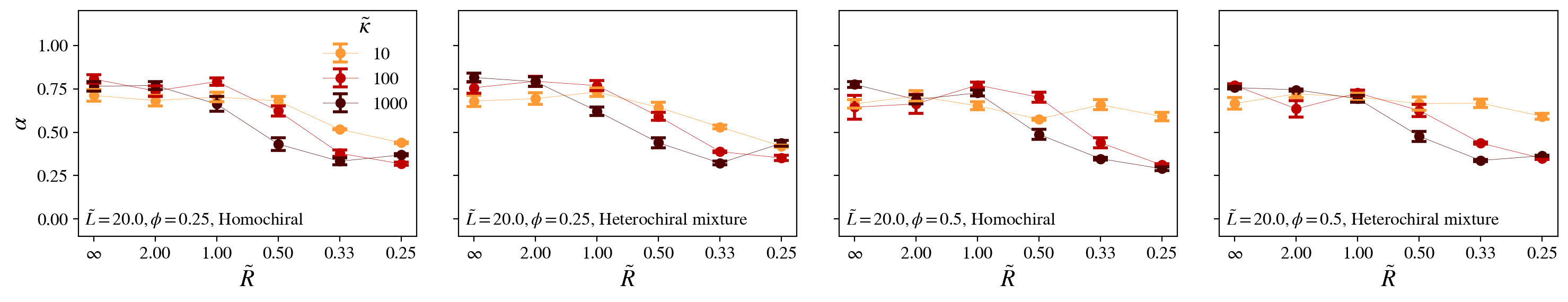
Figure 5: Values of the exponential scaling $\alpha$ for the number fluctuations in the system $\Delta N\propto\langle N\rangle^{\alpha}$ plotted as a function of $\tilde{R}$ for all simulation parameters. Top row plots are for filaments with aspect ratio $\tilde{L}=10$ and the bottom row $\tilde{L}=20$.

VI Identification of filament clusters

To quantify the dynamics and structure of the filament clusters, filaments were clustered by their centers of curvature $\mathbf{r}_{c}(t)$, determined from the filaments’ instantaneous radius of curvature $R(t)$ averaged over the contour length of the filament. Cluster positions are defined to be the average of their constituent filament centers of curvature, $\mathbf{r}_{C}(t)=\frac{1}{n}\sum_{i}^{n}\mathbf{r}_{c}^{(i)}(t)$, and the cluster radii are defined to be the average of the constituent filament curvature radii $R_{c}(t)=\frac{1}{n}\sum_{i}^{n}R_{i}(t)$.

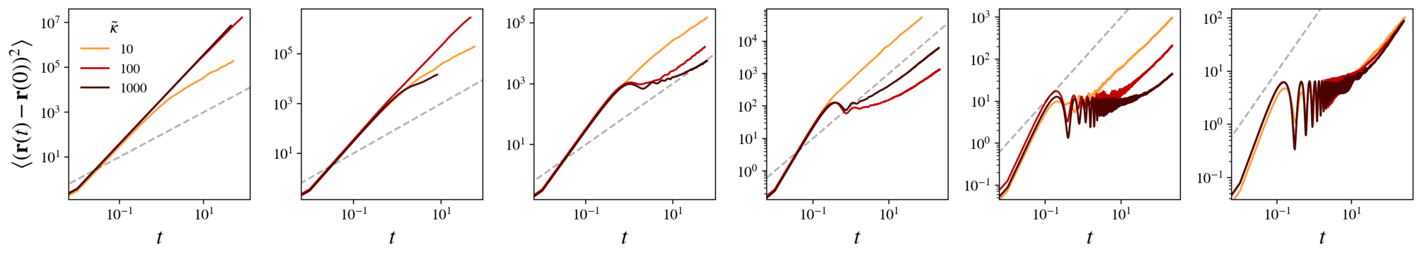
Figure 6: Mean-squared displacements (MSDs) plotted for $\tilde{L}=10$ for heterochiral systems with $\phi=0.25$, showing the short- and long-time scaling behavior. The effective diffusion coefficent $D_{\text{active}}$ was found by fitting the final $25\tau_{A}$ of the MSD.

Unclustered filaments can join an existing cluster when $|\mathbf{r}_{c}^{(i)}(t)-\mathbf{r}_{C}(t)|\leq R_{c}(t)$ for a time interval of $\tau_{A}$. Two previously unclustered filaments can form a new cluster if their centers of curvature are bounded by the average of their curvature radii, $|\mathbf{r}_{c}^{(i)}(t)-\mathbf{r}_{c}^{(j)}(t)|<(R_{i}(t)+R_{j}(t))/2$ for a minimum time interval of $\tau_{A}$. Filaments can leave a cluster if their center of curvature leaves the bounded space defined by the curvature position and curvature radius for an interval of $0.25\tau_{A}$, or if ever the filament center of curvature is no longer oriented in the direction of the cluster position, $(\mathbf{r}_{c}(t)-\mathbf{r}_{i}(t))\cdot(\mathbf{r}_{C}(t)-\mathbf{r}_{i}(t))<0$. A cluster is annihilated if ever the number of filaments in the cluster is less than 2.

Fig. 7 compares the average cluster radius $\langle\tilde{R}\rangle$ (normalized by the filament length) for homochiral and heterochiral systems. At large filament curvature radii, slightly larger clusters appear to be possible, which are perhaps limited by finite size effects. However, there does not appear to be a significantly different cluster scaling between heterochiral and homochiral systems.

VII Randomness of filament clusters

We assessed whether the clusters of filaments with small radius of curvature $\tilde{R}\leq 0.5$ sorted macroscopically into larger domains of homochiral clusters by measuring the mixing between left-handed (LH) and right-handed (RH) clusters. Upon identifying the cluster positions, described above, we constructed an adjacency matrix $X$ representing a graph with cluster centers as vertices and edges joining the cluster nearest neighbors. In a well-mixed (random) system, the handedness of nearest neighbors for any one vertex should be $\pm 1$ with equal probabilities. This would imply that each vertex of $X$ would have adjacent neighbors with a net handedness $\Sigma=\sum_{i}^{\text{adj}}\chi_{i}$ that should be zero on average but with normal variance from a randomly distributed network. In a system with sorted domains, the nonrandom distribution of handedness among clusters would give rise to a bimodal distribution of $\Sigma$, and a nonrandom lattice with approximately alternating handedness would be unimodal with zero mean and very small variance.

In Fig. 8 the distribution of $\Sigma$ (right) associated with the simulation image (left) is shown in red. The distribution appears normal with zero mean, and is contrasted with distributions of $\Sigma$ for nonrandom distributions of handedness. The adjacency graph associated with the image is plotted in the center. There does not appear to be any sign of macroscopic sorting in the distribution, so we must conclude that the distribution of handedness among the clusters is random. This approach was repeated for different simulation parameters, without any indication of nonrandomness.

VIII Diagrams of simulation images

Figs. 9–12 are diagrams of simulation images for the collective behavior displayed for varying $\tilde{R}$ and $\tilde{\kappa}$ for homochiral and heterochiral filaments at filament densities $\phi=0.25$ and $0.5$ and filament aspect ratios $\tilde{L}=10$ and $20$.

Noteably, Fig. 9 and Fig. 12 have images of filaments with $\tilde{R}=2$ that highlight the breakdown of long-range polar order for rigid filaments ($\tilde{\kappa}=1000$) due to the filament packing, as mentioned in the main text.

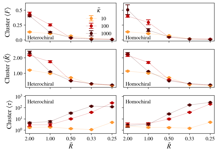
Figure 7: Top row: the fraction of simulation filaments in an average cluster $\langle F\rangle$ for homochiral and heterochiral systems. Center row: average cluster radius $\langle\tilde{R}\rangle$ plotted for homochiral and heterochiral systems. Bottom row: Average cluster lifetime $\langle\tau\rangle$ for homochiral and heterochiral systems plotted with respect to radius of curvature. Lifetimes are expressed in units of $\tau_{A}$.

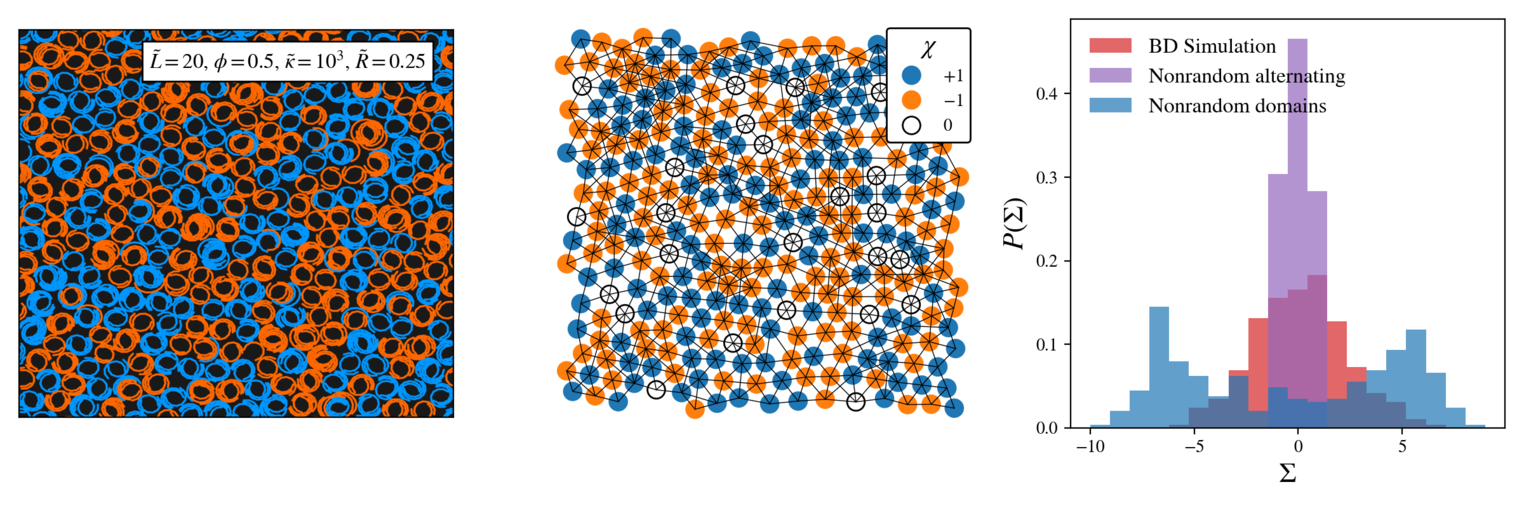
Figure 8: Left: simulation image for a heterochiral mixture of homochiral clusters. Center: The associated adjacency graph joining the centers of clusters to their nearest neighbors, with with clusters of mixed handedness being assigned a handedness of zero. The graph does not show edges between vertices across periodic boundaries, although these edges were present in our analysis. Right: the distribution of the sum of neighbor handedness $\Sigma$ for each vertex, plotted for the associated simulation to the left (shown in red), contrasted with distributions for the same adjacency graph with hypothetical nonrandom handedness distributions.

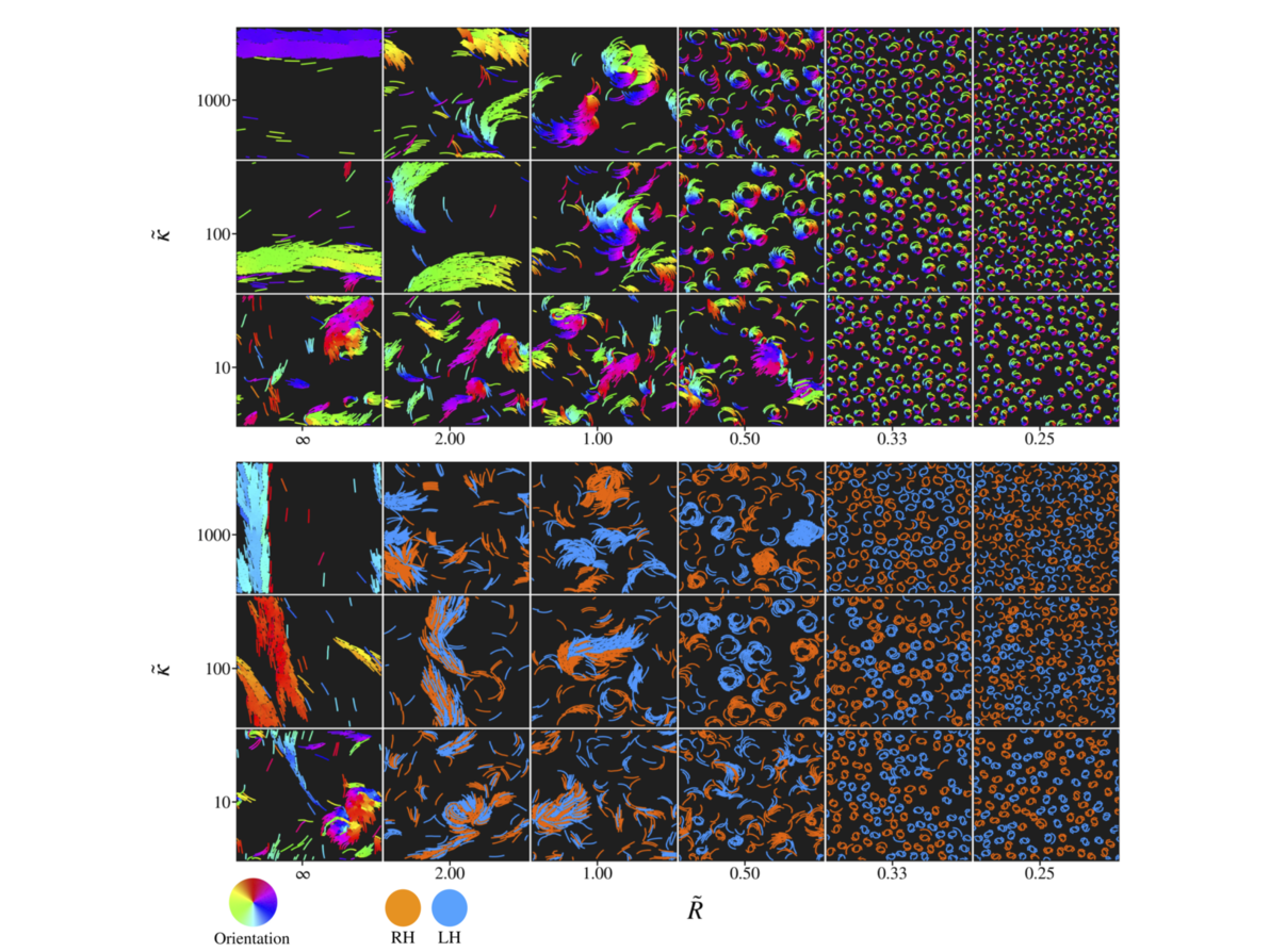
Figure 9: Simulation images for filaments with $\tilde{L}=10$ and packing fraction $\phi=0.25$ for homochiral (top) and heterochiral (bottom) systems.

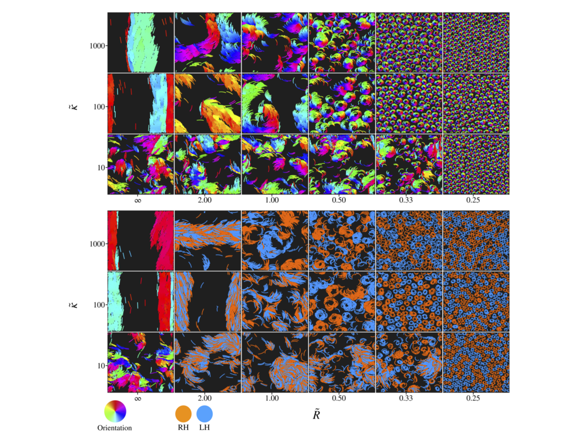
Figure 10: Simulation images for filaments with $\tilde{L}=10$ and packing fraction $\phi=0.50$ for homochiral (top) and heterochiral (bottom) systems.

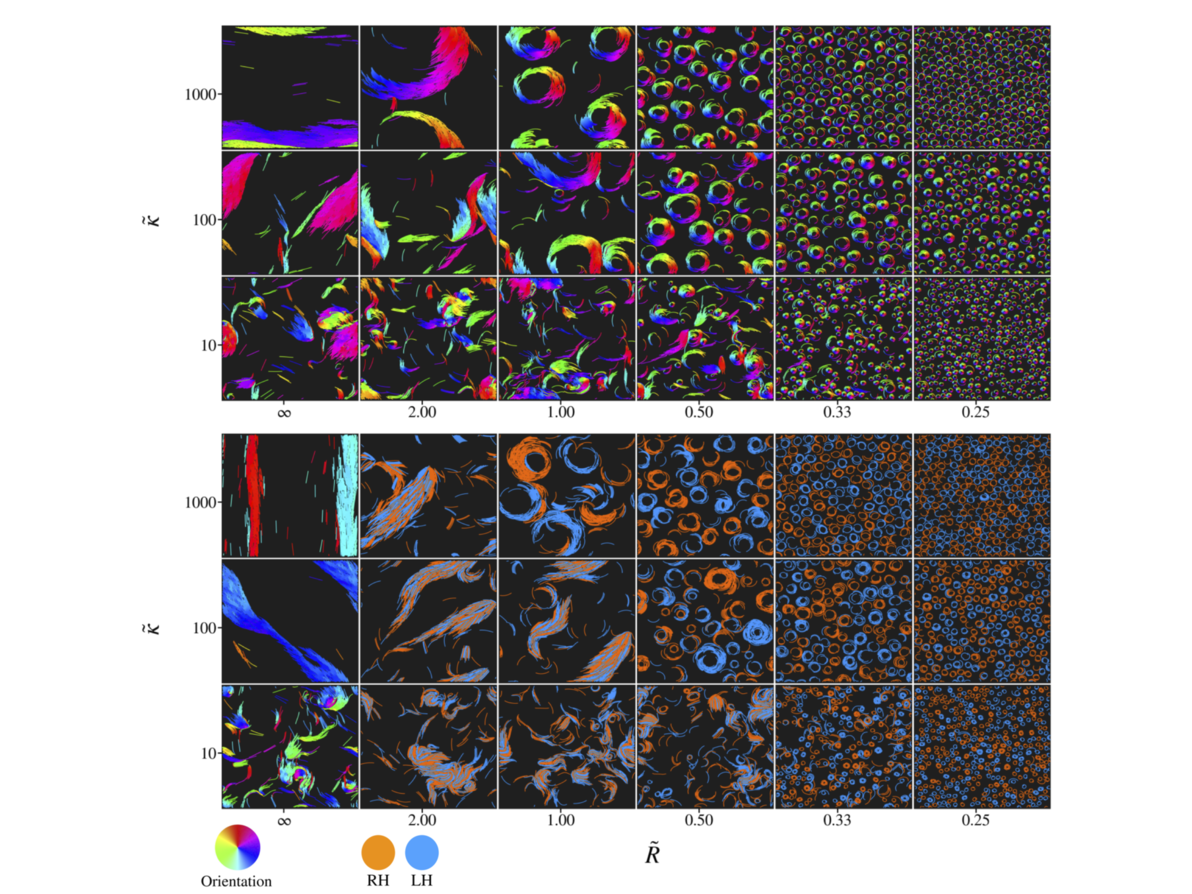
Figure 11: Simulation images for filaments with $\tilde{L}=20$ and packing fraction $\phi=0.25$ for homochiral (top) and heterochiral (bottom) systems.

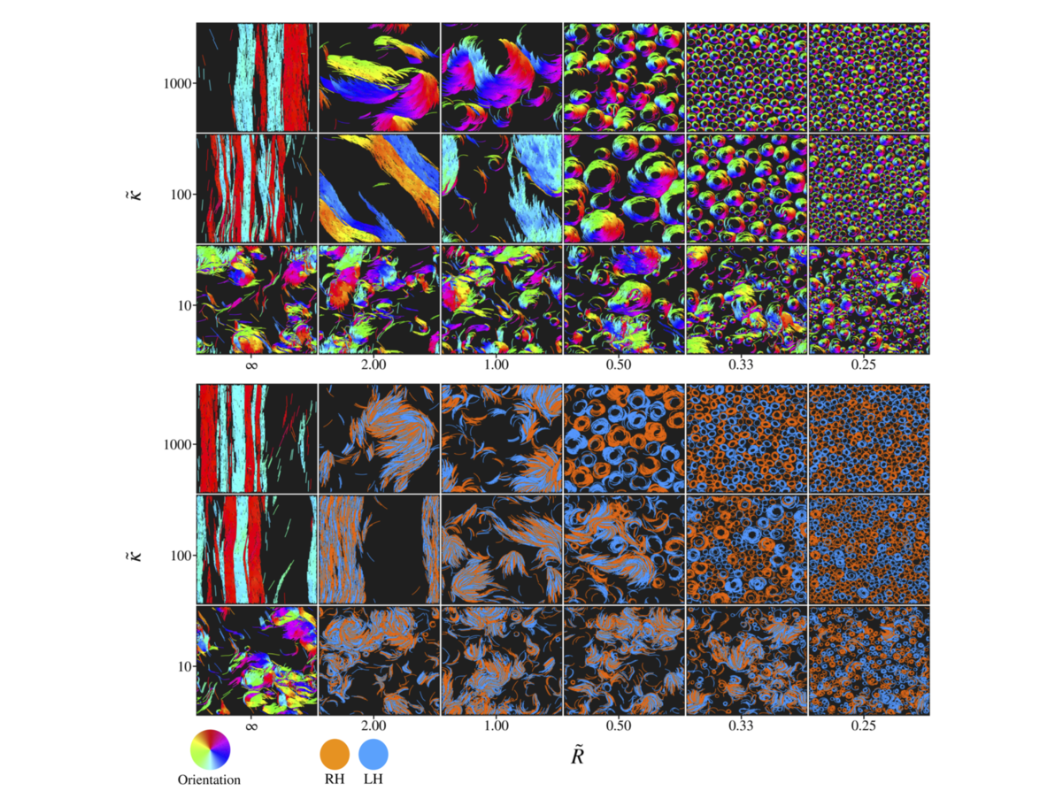
Figure 12: Simulation images for filaments with $\tilde{L}=20$ and packing fraction $\phi=0.50$ for homochiral (top) and heterochiral (bottom) systems.

References

- [1] O. Kratky and G. Porod. Röntgenuntersuchung gelöster Fadenmoleküle. Recueil des Travaux Chimiques des Pays-Bas, 68(12):1106–1122, 1949.
- [2] Alberto Montesi, David C. Morse, and Matteo Pasquali. Brownian dynamics algorithm for bead-rod semiflexible chain with anisotropic friction. The Journal of Chemical Physics, 122(8):084903, February 2005.
- [3] Jeffrey M. Moore. C-GLASS: A Coarse-Grained Living Active Systems Simulator. Zenodo, May 2020. 10.5281/zenodo.3841613.
- [4] Jeffrey M. Moore, Tyler N. Thompson, Matthew A. Glaser, and Meredith D. Betterton. Collective motion of driven semiflexible filaments tuned by soft repulsion and stiffness. arXiv:1909.11805, May 2020.
- [5] Masao Doi and S. F. Edwards. The Theory of Polymer Dynamics. Clarendon Press, 1988.
- [6] L.D. Landau, E.M. Lifshitz, A.M. Kosevich, J.B. Sykes, L.P. Pitaevskii, and W.H. Reid. Theory of Elasticity: Volume 7. Course of Theoretical Physics. Elsevier Science, 1986.
- [7] Marshall Fixman. Simulation of polymer dynamics. I. General theory. The Journal of Chemical Physics, 69(4):1527–1537, August 1978.
- [8] Matteo Pasquali and David C. Morse. An efficient algorithm for metric correction forces in simulations of linear polymers with constrained bond lengths. The Journal of Chemical Physics, 116(5):1834–1838, January 2002.
- [9] Lynn Liu, Erkan Tüzel, and Jennifer L Ross. Loop formation of microtubules during gliding at high density. Journal of Physics: Condensed Matter, 23(37):374104, September 2011.
- [10] Jonathon Anderson, Patrick J. Burns, Daniel Milroy, Peter Ruprecht, Thomas Hauser, and Howard Jay Siegel. Deploying RMACC Summit: An HPC Resource for the Rocky Mountain Region. In Proceedings of the Practice and Experience in Advanced Research Computing 2017 on Sustainability, Success and Impact, PEARC17, pages 8:1–8:7, New York, NY, USA, 2017. ACM.
- [11] Rolf E. Isele-Holder, Jens Elgeti, and Gerhard Gompper. Self-propelled worm-like filaments: Spontaneous spiral formation, structure, and dynamics. Soft Matter, 11(36):7181–7190, 2015.
- [12] Shalabh K. Anand and Sunil P. Singh. Structure and dynamics of a self-propelled semiflexible filament. Physical Review E, 98(4):042501, October 2018.
- [13] Nisha Gupta, Abhishek Chaudhuri, and Debasish Chaudhuri. Morphological and dynamical properties of semiflexible filaments driven by molecular motors. Physical Review E, 99(4):042405, April 2019.
- [14] Matthew S. E. Peterson, Michael F. Hagan, and Aparna Baskaran. Statistical properties of a tangentially driven active filament. Journal of Statistical Mechanics: Theory and Experiment, 2020(1):013216, January 2020.
- [15] Guillaume Grégoire and Hugues Chaté. Onset of Collective and Cohesive Motion. Physical Review Letters, 92(2):025702, January 2004.
- [16] Hugues Chaté, Francesco Ginelli, Guillaume Grégoire, and Franck Raynaud. Collective motion of self-propelled particles interacting without cohesion. Physical Review E, 77(4):046113, April 2008.
- [17] Francesco Ginelli, Fernando Peruani, Markus Bär, and Hugues Chaté. Large-Scale Collective Properties of Self-Propelled Rods. Physical Review Letters, 104(18):184502, May 2010.
- [18] Francesco Ginelli. The Physics of the Vicsek model. The European Physical Journal Special Topics, 225(11):2099–2117, November 2016.