The Optimal ‘AND’

Abstract

The joint distribution $P(X,Y)$ cannot be determined from its marginals $P(X)$ and $P(Y)$ alone; one also needs one of the conditionals $P(X|Y)$ or $P(Y|X)$. But is there a best guess, given only the marginals? Here we answer this question in the affirmative, obtaining in closed form the function of the marginals that has the lowest expected Kullbach-Liebler (KL) divergence between the unknown “true” joint probability and the function value. The expectation is taken with respect to Jeffreys’ non-informative prior over the possible joint probability values, given the marginals. This distribution can also be used to obtain the expected information loss for any other aggregation operator, as such estimators are often called in fuzzy logic, for any given pair of marginal input values. This enables such such operators, including ours, to be compared according to their expected loss under the minimal knowledge conditions we assume.

We go on to develop a method for evaluating the expected accuracy of any aggregation operator in the absence of knowledge of its inputs. This requires averaging the expected loss over all possible input pairs, weighted by an appropriate distribution. We obtain this distribution by marginalizing Jeffreys’ prior over the possible joint distributions (over the 3 functionally independent coordinates of the space of joint distributions over two Boolean variables) onto a joint distribution over the pair of marginal distributions, a 2-dimensional space with one parameter for each marginal. We report the resulting input-averaged expected losses for a few commonly used operators, as well as the optimal operator.

Finally, we discuss the potential to develop our methodology into a principled risk management approach to replace the often rather arbitrary conditional-independence assumptions made for probabilistic graphical models.

1 Introduction

Given truth values for propositions $X$ and $Y$, the truth value of the conjunction $X\wedge Y$ is fully determined by the truth table for the logical connective ‘AND’. But if we are only able to assign non-extremal probabilities $P(X)$ and $P(Y)$ to these propositions, then the joint probability $P(X\wedge Y)$ is not fully determined. Further information such as the conditional probability $P(Y|X)$ is required. The essence of the problem is that the space of joint distributions over two Boolean values has three dimensions, of which the marginals are only able to constrain two. Nevertheless, some guesses are better than others. Under Bayesian principles [jaynes03, Caticha:2008eso], the best guess is the one that minimizes the expected information loss under the distribution that maximizes the entropy over what is not known, given whatever is known. Here we apply this principle to obtain an optimal estimate for $P(X\wedge Y)$ given $P(X)$ and $P(Y)$. We apply the principle again under the still more information-sparse conditions of knowing neither $P(X)$ nor $P(Y)$ to obtain the expected information loss for any given aggregation operator that estimates $P(X\wedge Y)$ from these marginals.

It is important to notice that we are not directly concerned with whether propositions $X$ and $Y$ hold true; the incompletely known variables in our chosen problems are probability distributions over the four possible joint outcomes of these two Boolean variables. To describe our state of knowledge about these distributions, we must work at the meta-level in which events take values within the space of such distributions, and concern ourselves with distributions over these distribution spaces. Unlike a finite set, which supports a trivial concept of uniformity, this event space forms a continuum, so entropy can be defined only with respect to some fiducial distribution that defines uniformity. In spaces of distributions, the uniquely qualified candidate for this meta-distribution is Jeffreys’ non-informative prior. It is proportional to the square root of determinant of the Fisher information metric, which in turn measures the distinguishibility of infinitesimally nearby distributions in the space. A crash course in these information-geometric topics can be found in Appendix A. Given this apparatus, maximum entropy problems become well-formulated as minimum Kullbach-Liebler divergence (KL) problems.

2 Formulation

We begin by introducing coordinates $\theta$ for the space of joint categorical distributions over two Boolean variables:

$$\theta_{11} =P(X,Y)$$ (1)

$$\theta_{10} =P(X,\neg Y)$$ (2)

$$\theta_{01} =P(\neg X,Y)$$ (3)

The coordinates range over the 3-simplex defined by

$$\theta_{11} \geq 0$$ (4)

$$\theta_{10} \geq 0$$ (5)

$$\theta_{01} \geq 0$$ (6)

$$\theta_{11}+\theta_{10}+\theta_{01} \leq 1$$ (7)

We also introduce the function

$$\theta_{00}(\theta)=1-\theta_{11}-\theta_{10}-\theta_{01}$$ (8)

which is not to be confused with one of the 3 coordinates, even when written as $\theta_{00}$ without making its argument explicit.

In this coordinate system, we obviously have

$$P(X) =\theta_{11}+\theta_{10}$$ (9)

$$P(Y) =\theta_{11}+\theta_{01}$$ (10)

Abbreviating $P(X)$ as $a$ and $P(Y)$ as $b$, our knowledge can be expressed by the constraints

$$\theta_{11}+\theta_{10} =a$$ (11)

$$\theta_{11}+\theta_{01} =b$$ (12)

Let us use these constraints to eliminate the coordinates $\theta_{10}$ and $\theta_{01}$:

$$\theta_{10} =a-\theta_{11}$$ (13)

$$\theta_{01} =b-\theta_{11}$$ (14)

The range restrictions (4), (5), (6) and (7) then become

$$\theta_{11} \geq 0 \theta_{11} \geq 0$$ (16)

$$a-\theta_{11} \geq 0 \qquad\theta_{11} \leq a$$ (17)

$$b-\theta_{11} \geq 0 \qquad\theta_{11} \leq b$$ (18)

$$\theta_{11}+a-\theta_{11}+b-\theta_{11} \leq 1 \qquad\theta_{11} \geq a+b-1$$ (19)

which can be summarized as

$$\theta_{\downarrow} \leq\theta_{11}\leq\theta_{\uparrow}$$ (20)

$$\theta_{\downarrow} =\max(a+b-1,0)$$ (21)

$$\theta_{\uparrow} =\min(a,b)$$ (22)

3 The optimal estimate

In Appendix A, we motivate and derive the Fisher information matrix and the measure that it defines over spaces of probability distributions. In the present case, the Fisher information matrix has the single element

$$g_{(11),(11)}(\theta_{11}) =\sum_{x\in\{T,F\}}P(x|\theta_{11})[\partial_{\theta_{11}}\ln P(x|\theta_{11})][\partial_{\theta_{11}}\ln P(x|\theta_{11})]$$

$$=\theta_{11}\theta_{11}^{-2}+(1-\theta_{11})(-(1-\theta_{11}))^{-2}$$

$$=\theta_{11}^{-1}+(1-\theta_{11})^{-1}=1/(\theta_{11}(1-\theta_{11}))$$ (24)

The “uniform” measure over this space, Jeffreys’ non-informative prior, is the square root of the determinant of $g$, which is just $1/\sqrt{\theta_{11}(1-\theta_{11})}$. This is essentially the Beta(${\scriptstyle\frac{1}{2}},{\scriptstyle\frac{1}{2}}$) density, except that its support is limited to a sub-interval of the unit interval. The integral over this support region, which gives the normalization constant needed to convert this measure into a probability measure, is an incomplete Beta function for which we have a special case that reduces to

$$Z =\int_{\theta_{\downarrow}}^{\theta_{\uparrow}}\frac{dx}{\sqrt{x(1-x)}}=2\sin^{-1}(\sqrt{x})\biggr{|}_{\theta_{\downarrow}}^{\theta_{\uparrow}}$$

$$=2\sin^{-1}\bigl{(}\sqrt{\theta_{\uparrow}}\bigr{)}-2\sin^{-1}\bigl{(}\sqrt{\theta_{\downarrow}}\bigr{)}$$ (25)

which is plotted in Figure 1.

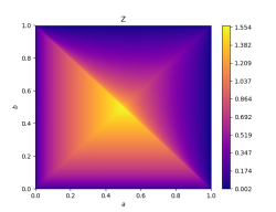
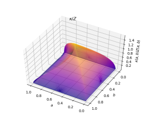
Figure 1: The normalization factor $Z$ (25) as a function of the marginals. The discontinuities of (21) and (22) are prominently reflected.

To see this, recall the standard result $d\sin^{-1}(x)/dx=1/\sqrt{1-x^{2}}$ and observe that

$$\frac{d}{dx}2\sin^{-1}(\sqrt{x})=\frac{2}{\sqrt{1-x}}\frac{1}{2\sqrt{x}}=\frac{1}{\sqrt{x(1-x)}}.$$ (26)

We therefore conclude that $\theta_{11}$ is distributed between $\theta_{\downarrow}$ and $\theta_{\uparrow}$ according to the density

$$P(\theta_{11})=\frac{1}{Z}\frac{1}{\sqrt{(\theta_{11}(1-\theta_{11}))}}$$ (27)

with $Z$ given by (25).

With this distribution in hand, we can derive an optimal estimate $\theta_{11}^{*}(a,b)$ for $\theta_{11}$. Suppose we institute a policy of using some fixed function $f(a,b)$ to estimate $\theta_{11}$. Then the expected KL divergence between this estimate and $\theta_{11}$ would be

$$KL[\theta_{11},f(a,b)] =\theta_{11}\ln\frac{\theta_{11}}{f(a,b)}+(1-\theta_{11})\ln\frac{1-\theta_{11}}{1-f(a,b)}$$ (28)

where we choose to weight the log likelihood ratio by the true distribution $\theta_{11}$, not the estimated distribution $f(a,b)$. The expected information loss is therefore the expectation value of (28) under distribution (27). Abbreviating $f(a,b)$ as $x$ and $\theta_{11}$ as $\xi$, this is

$$\langle KL[\theta_{11},f(a,b)]\rangle_{\theta_{11}} =\frac{\kappa}{Z}-\frac{A}{Z}\ln x-\frac{B}{Z}\ln(1-x)$$ (29)

$$\kappa =\int_{\theta_{\downarrow}}^{\theta_{\uparrow}}d\xi\frac{\xi\ln\xi+(1-\xi)\ln(1-\xi)}{\sqrt{\xi(1-\xi)}}$$ (30)

$$A =\int_{\theta_{\downarrow}}^{\theta_{\uparrow}}d\xi\sqrt{\xi/(1-\xi)}$$ (31)

$$B =\int_{\theta_{\downarrow}}^{\theta_{\uparrow}}d\xi\sqrt{(1-\xi)/\xi}$$ (32)

Note that with the change of variable $\xi^{\prime}=1-\xi$, $d\xi^{\prime}=-d\xi$, (32) becomes $B=-\int_{1-\theta_{\downarrow}}^{1-\theta_{\uparrow}}d\xi^{\prime}\sqrt{\xi^{\prime}/(1-\xi^{\prime})}=\int_{1-\theta_{\uparrow}}^{1-\theta_{\downarrow}}d\xi^{\prime}\sqrt{\xi^{\prime}/(1-\xi^{\prime})}$, so $A$ and $B$ involve the same indefinite integral, verified in Appendix B.1 (81) to be:

$$\int d\xi\sqrt{\frac{\xi}{1-\xi}}=\tan^{-1}(\sqrt{\xi/(1-\xi)})-\sqrt{\xi(1-\xi)}.$$ (34)

This gives

$$A= \tan^{-1}\Bigl{(}\sqrt{\theta_{\uparrow}/(1-\theta_{\uparrow})}\Bigr{)}-\tan^{-1}\Bigl{(}\sqrt{\theta_{\downarrow}/(1-\theta_{\downarrow})}\Bigr{)}$$

$$-\sqrt{\theta_{\uparrow}(1-\theta_{\uparrow})}+\sqrt{\theta_{\downarrow}(1-\theta_{\downarrow})}.$$ (35)

$$B= \tan^{-1}\Bigl{(}\sqrt{(1-\theta_{\downarrow})/\theta_{\downarrow}}\Bigr{)}-\tan^{-1}\Bigl{(}\sqrt{(1-\theta_{\uparrow})/\theta_{\uparrow}}\Bigr{)}$$

$$-\sqrt{(1-\theta_{\downarrow})\theta_{\downarrow}}+\sqrt{(1-\theta_{\uparrow})\theta_{\uparrow}}.$$ (36)

We note that $A$ and $B$ are both non-negative because the integrand of (34) is non-negative and in each case the integral is taken in a positive sense.

The two terms in $\kappa$ (30) can be similarly written in terms of a single indefinite integral, but one that does not have a simple expression in terms of elementary functions. (It can be expressed in terms of a generalized hypergeometric function, but we do not pursue this here.) It was integrated numerically to obtain the plot in Figure 2. We note that $\kappa\leq 0$, as is clear from (30). This term does not depend on the estimate $x=f(a,b)$, and in this sense is a constant contribution to the expected information loss.

The optimal estimate $\theta_{11}^{*}(a,b)$ minimizes the expected loss (29). Setting its derivative with respect to $x$ to zero gives

$$\frac{A}{x}-\frac{B}{1-x} =0$$

$$A-Ax =Bx$$

$$x =\theta_{11}^{*}(a,b)=A/(A+B)$$ (37)

We note that $A+B$ contains only the $\tan^{-1}$ terms of (35) and (36).

Because $A$ and $B$ are non-negative, we see that the optimal estimate (37) lies between 0 and 1, as it should. To confirm that the extremum (37) is indeed a minimum, we note that the second derivative of (29) is proportional to

$$\frac{A}{x^{2}}+\frac{B}{(1-x)^{2}}\geq 0.$$ (38)

Plugging $x$ from (37) into (29) gives the expected loss for the optimal estimate:

$$\langle KL[\theta_{11},\theta_{11}^{*}(a,b)]\rangle_{\theta_{11}} =\frac{\kappa}{Z}-\frac{A}{Z}\ln\frac{A}{A+B}-\frac{B}{Z}\ln\frac{B}{A+B}$$

$$=\bigl{(}\kappa-A\ln A-B\ln B+(A+B)\ln(A+B)\bigr{)}/Z$$ (39)

The optimal estimate (37) is plotted along with its expected loss (39) in Figure 3.

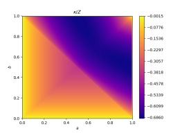
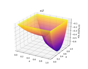
Figure 2: The aggregation-operator-independent term $\kappa/Z$ (30,25) as a function of the input marginals. Contour plot on the right, 3d plot on the left.

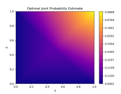
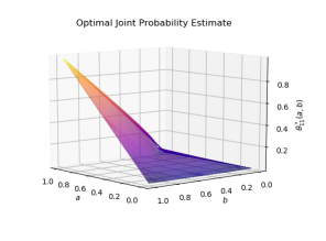
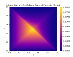
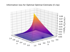
Figure 3: The optimal aggregation operator (37). Contour plot on upper left, 3D plot on upper right. Corresponding information loss costs in lower two plots. These include the aggregation-operator-independent term $\kappa$ (30) shown in Figure 2, which was obtained by numerical integration. Small inaccuracies in this integration resulted in small negative values for the expected KL cost, which are not mathematically possible. These were truncated to 0.

4 Aggregation operator cost

Expression (37), together with (35), (36), (21) and (22) gives the optimal estimate $P(X,Y)$ given that $P(X)=a$ and $P(X)=b$. Given a different estimate $f(a,b)$, of which a considerable variety are in use [Detyniecki:01:Aggregation], one can apply (29) and compare the result to (39) to determine how much worse the sub-optimal estimate is for any particular marginals $a$ and $b$.

In order to judge how well an aggregation formula $f$ works in general, without committing to any particular values of its arguments, we need to average the expected loss of the estimate over all marginal values $a$ and $b$ under a non-informative distribution. To obtain this distribution over $(a,b)$, we assume Jeffreys’ non-informative prior over the joint distributions $\theta=(\theta_{11},\theta_{01},\theta_{10})$, apply (11) and (12) to transform to coordinates that eliminate $\theta_{01}$ and $\theta_{10}$ in favor of $a$ and $b$, and integrate out $\theta_{11}$.

As derived in Appendix A, Jeffreys’ prior over the joint distributions is the Dirichlet distribution:

$$P(\theta)=\pi^{-2}(\theta_{11}\theta_{10}\theta_{01}\theta_{00})^{-{\scriptstyle\frac{1}{2}}}$$ (40)

To change to coordinates $\phi\equiv(\theta_{11},a,b)$, we must not only substitute (13) and (14) into (40), but also ensure that $P(\theta)d^{3}\theta=P(\phi)d^{3}\phi$ by dividing $P(\theta)$ by the absolute value of the Jacobian determinant

$$\begin{vmatrix}\frac{\partial\phi}{\partial\theta}\end{vmatrix}=\begin{vmatrix}\frac{\partial\theta_{11}}{\partial\theta_{11}}&\frac{\partial a}{\partial\theta_{11}}&\frac{\partial b}{\partial\theta_{11}}\\ \frac{\partial\theta_{11}}{\partial\theta_{01}}&\frac{\partial a}{\partial\theta_{01}}&\frac{\partial b}{\partial\theta_{01}}\\ \frac{\partial\theta_{11}}{\partial\theta_{10}}&\frac{\partial a}{\partial\theta_{10}}&\frac{\partial b}{\partial\theta_{10}}\end{vmatrix}=\begin{vmatrix}1&1&1\\ 0&0&1\\ 0&1&0\end{vmatrix}=-1.$$ (41)

However, this turns out to be an immaterial unit factor, so we have

$$P(\phi) =\pi^{-2}\bigl{(}\theta_{11}(a-\theta_{11})(b-\theta_{11})(1-\theta_{11}-(a-\theta_{11})-(b-\theta_{11})\bigr{)}^{-{\scriptstyle\frac{1}{2}}}$$

$$=\pi^{-2}\bigl{(}\theta_{11}(a-\theta_{11})(b-\theta_{11})(1+\theta_{11}-a-b)\bigr{)}^{-{\scriptstyle\frac{1}{2}}}$$ (42)

The marginal over $a$ and $b$ is then found by integrating out $\theta_{11}$:

$$P(a,b) =\pi^{-2}\int_{\theta_{\downarrow}}^{\theta_{\uparrow}}d\theta_{11}\bigl{(}\theta_{11}(a-\theta_{11})(b-\theta_{11})(1+\theta_{11}-a-b)\bigr{)}^{-{\scriptstyle\frac{1}{2}}}.$$ (43)

This is an incomplete elliptic integral of the first kind. With the definition

$$K(\phi,m)=\int_{0}^{\phi}(1-m\sin^{2}\theta)^{-{\scriptstyle\frac{1}{2}}}d\theta\qquad 0\leq m\leq 1,\quad 0\leq\phi\leq\frac{\pi}{2}$$ (44)

and substituting $x=\theta_{11}$, the antiderivative of the integrand $\pi^{-2}\bigl{(}x(a-x)(b-x)(1+x-a-b)\bigr{)}^{-{\scriptstyle\frac{1}{2}}}$ in (43) is

$$I(x;a,b)=\frac{2}{\pi^{2}}\frac{b-a}{|b-a|}\frac{1}{\sqrt{b(1-b)}}K\Biggl{(}\sin^{-1}\Biggl{(}\sqrt{\frac{(1-b)(b-x)}{(1-a)(a-x)}}\Biggr{)},\frac{a(1-a)}{b(1-b)}\Biggr{)}$$ (45)

as verified in Appendix B.2. However, if we attempt to obtain the definite integral (43) simply by plugging in the limits, we may find ourselves in violation of the conditions $0\leq m<1$ and $0\leq\phi\leq\pi/2$. Inspecting (45), we see that

$$m =\frac{a(1-a)}{b(1-b)}$$ (46)

$$\sin^{2}\phi =\frac{(1-b)(b-x)}{(1-a)(a-x)}.$$ (47)

The non-negativity constraint on $m$ is always satisfied, because $a$ and $b$ are probabilities lying between $0$ and $1$. But the upper bound is problematic when $b$ is near either end of its allowed range. That condition can be written

$$\frac{a(1-a)}{b(1-b)} <1$$

$$a-a^{2} <b-b^{2}$$

$$0 <b-a-(b^{2}-a^{2})=(b-a)-(b-a)(b+a)$$

$$0 <(b-a)(1-b-a)$$

$$(b>a\text{ and }a+b<1) \text{ or }(b<a\text{ and }a+b>1)$$ (48)

The remaining condition amounts to $0\leq\frac{(1-b)(b-x)}{(1-a)(a-x)}\leq 1$. Because $a$ and $b$ are marginal probabilities that include $x$ (i.e., $\theta_{11}$) within their mass, we have $b-x\geq 0$ and $a-x\geq 0$, so the non-negativity constraint is satisfied. The remaining constraint is

$$\frac{(1-b)(b-x)}{(1-a)(a-x)} \leq 1$$

$$a-x-a^{2}+ax \geq b-x-b^{2}+bx$$

$$0 \geq(b-a)-(b^{2}-a^{2})+(b-a)x=(b-a)(1-a-b+x)$$

$$0 \leq(b-a)(a+b-1-x)$$

$$(b\geq a\text{ and }x\leq a+b-1) \text{ or }(b\leq a\text{ and }x\geq a+b-1)$$ (49)

Combining these conditions with (48) has the consequences

$$(b\geq a\text{ and }x\leq 0)\text{ or }(b\leq a\text{ and }x\geq 0)$$ (50)

so because $x\geq 0$ we conclude that we can proceed only if $b\leq a$, in which case (48) implies that we must also restrict consideration to $a+b>1$.

It remains to determine whether the second condition in (49), $x\geq a+b-1$, is respected by the limits $x=\theta_{\uparrow}=\min(a,b)$ and $x=\theta_{\downarrow}=\max(a+b-1,0)$. For $\theta_{\uparrow}$, having already restricted to $b\leq a$, we have

$$\min(a,b) \geq a+b-1$$

$$b \geq a+b-1$$

$$1 \geq a$$ (51)

which is always satisfied. Moving on to $\theta_{\downarrow}$ we obtain

$$\max(a+b-1,0) \geq a+b-1.$$ (52)

which, having restricted attention to $a+b>1$, is always satisfied.

Leaving aside the question of how to handle the remaining cases, let us plug the limits into (45). At $x=\theta_{\uparrow}=\min(a,b)=b$, the argument of $K$ vanishes, so as is clear from (44), so does $K$. This leaves the lower limit $x=\theta_{\downarrow}=\max(a+b-1,0)=a+b-1$ (with the $a+b>1$ constraint), at which we see

$$\frac{(1-b)(b-x)}{(1-a)(a-x)} =\frac{(1-b)(b-(a+b-1))}{(1-a)(a-(a+b-1))}=\frac{(1-b)(1-a)}{(1-a)(1-b)}=1$$ (53)

Thus, we obtain

$$P(a,b)=\frac{2}{\pi^{2}}\frac{1}{b(1-b)}K\Bigl{(}\frac{\pi}{2},\frac{a(1-a)}{b(1-b)}\Bigr{)}$$ (54)

for $b<a$ and $a+b>1$. Let us call this expression $P^{<>}(a,b)$ to remind us of these two conditions.

The remaining cases can be obtained from the symmetries of (43). The most obvious is that $P(a,b)=P(b,a)$. Hence, for all $a$ and $b$ with $a+b>1$, we can say

$$P(a,b)=\begin{cases}P^{<>}(a,b)&[b<a]\\ P^{<>}(b,a)&[b>a]\end{cases}$$ (55)

leaving the $a+b<1$ cases to be determined.

Less obviously, $P(1-a,1-b)=P(a,b)$. Plugging into (43), we have

$$P(1-a,1-b) =\pi^{-2}\int_{\theta_{\downarrow}}^{\theta_{\uparrow}}d\theta_{11}\bigl{(}\theta_{11}(1-a-\theta_{11})(1-b-\theta_{11})$$

$$\qquad\qquad\qquad\qquad(1+\theta_{11}-(1-a)-(1-b))\bigr{)}^{-{\scriptstyle\frac{1}{2}}}$$ (56)

$$=\pi^{-2}\int_{\theta_{\downarrow}}^{\theta_{\uparrow}}d\theta_{11}\bigl{(}\theta_{11}(1-a-\theta_{11})(1-b-\theta_{11})(a+b+\theta_{11}-1)\bigr{)}^{-{\scriptstyle\frac{1}{2}}}$$

Let $x^{\prime}=x+a+b-1$, so $x=x^{\prime}-a-b+1$. At the limit $x=\theta_{\uparrow}=\min(1-a,1-b)$ we have $x^{\prime}=\min(1-a,1-b)+a+b-1$. If $a<b$, this gives $x^{\prime}=a$, and if $b<a$ it gives $x^{\prime}=b$, so this limit becomes $\min(a,b)$, as in (43). At the limit $x=\theta_{\downarrow}=\max((1-a)+(1-b)-1,0)=\max(1-a-b,0)$, we have $x^{\prime}=\max(1-a-b,0)+a+b-1$. If $a+b>1$, this is $a+b-1$, and if $a+b<1$ it is $0$, so this limit becomes $\max{a+b-1,0}$, also agreeing with (43). Thus

$$P(1-a,1-b) =\pi^{-2}\int_{\theta_{\downarrow}}^{\theta_{\uparrow}}dx\bigl{(}x(1-a-x)(1-b-x)(a+b+x-1)\bigr{)}^{-{\scriptstyle\frac{1}{2}}}$$

$$=\pi^{-2}\int_{\theta_{\downarrow}}^{\theta_{\uparrow}}dx^{\prime}\bigl{(}(x^{\prime}-a-b+1)(1-a-(x^{\prime}-a-b+1))$$

$$\qquad\qquad(1-b-(x^{\prime}-a-b+1))(a+b+(x^{\prime}-a-b+1)-1)\bigr{)}^{-{\scriptstyle\frac{1}{2}}}$$

$$=\pi^{-2}\int_{\theta_{\downarrow}}^{\theta_{\uparrow}}dx^{\prime}(1+x^{\prime}-a-b)(b-x^{\prime})(a-x^{\prime})x^{\prime}$$

$$=P(a,b)$$ (57)

If $a+b<1$, then $(1-a)+(1-b)=2-(a+b)>1$, so we can use (57) to obtain $P(a,b)$. This density is plotted in Figure 4, which clearly shows the singularities at $a=b$ and $a+b=1$.

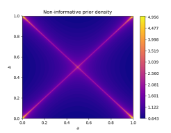
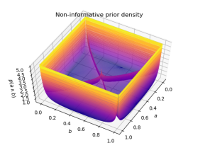
Figure 4: The non-informative prior distribution over the marginals. (57). Contour plot the left, 3D plot the right. The distribution is singular at every edge, and along the diagonal lines.

Method	Formula	Expected loss
Optimal	Eqn. (37)	0.0203
Product	$ab$	0.0272
Hamacher ($\gamma=0$)	$\frac{ab}{a+b-ab}$	0.0416
Min	$\min(a,b)$	0.0691
Lukasiewicz	$\max(a+b-1,0)$	0.5183

Table 1: Expected information loss for the optimal estimate and a few widely used t-norm aggregation operators.

The expected information loss (29) was integrated over this density using the optimal estimate (37) and a few other widely used t-norm aggregation operators taken from [Detyniecki:01:Aggregation] to write $x$ as a function of $a$ and $b$. The resulting overall expected losses are shown in Table 1.

Details of the numerical integration are given in Appendix C. The numerical procedure applied to the density (54, 55) alone integrated to 0.9989, so these figures should be accurate to roughly 0.1%.

5 Summary and future work

We have set out and demonstrated a principled method for deriving optimal aggregation formulas. The best-guess full joint distribution over two Boolean variables, given the marginal distributions, is given in closed form by (37), and its expected information loss, measured by Kullbach-Liebler divergence, is given by (39). Of course, if one has further information then the maximum entropy problem should be formulated differently, resulting in an improved guess.

We also set out and demonstrated a principled method for evaluating aggregation operators by their expected information loss, averaging over all their possible inputs. We applied the method to produce Table 1, listing the expected loss for the optimal aggregation operator and a few others. The method can be applied to extend the table to anyone’s favorite aggregation operator.

In probabilistic graphical model applications [bishopbook06], conditional independence assumptions are used to estimate joint distributions. These assumptions are often motivated more by practical limitations than by plausibility. At least in principle, it should be a better bet to take a quantitative risk management approach to dealing with such limitations, which is essentially what we have demonstrated in the simplest non-trivial case. One places the bet that has the lowest risk of being badly wrong, in the sense of expected information loss. Therefore it is of considerable interest to attempt to generalize the method in at least two ways: (i) from joint distributions over Boolean variables to joint-distributions over $n$-valued categorical variables for arbitrary $n>2$; and (ii) from joint distributions over two variables to distributions over greater numbers. On the latter point, with the machinery given here it is possible to treat the case of $n$ Boolean variables by repeated application of the 2-variable formula (37), but we see no good reason to believe that this would give the same result as minimization of expected KL loss within the space of $n$-variable distributions. It would also be of interest to extend the approach to commonly-used families of distributions over continuous spaces.

6 Acknowledgments

This work was carried out entirely with the author’s own time and resources, but benefitted from useful conversations with Elizabeth Rohwer and his SRI colleagues John Byrnes, Andrew Silberfarb and others on the Deep Adaptive Semantic Logic (DASL) team, supported in part by DARPA contracts HR001118C0023 and HR001119C0108 and SRI internal funding. All views expressed herein are the author’s own and are not necessarily shared by SRI or the US Government.

Appendices

Appendix A Fisher Information and Jeffreys’ prior

In this brief introduction to these topics in information geometry [amari93, Caticha_2015], we begin with the principle of invariance, which holds that any formula for comparing probability distributions should produce the same result under any one-to-one smooth invertable change of random variables. Otherwise the comparison would depend not purely on the distributions, but also on the coordinates used to express the random variables. This leads to the $\delta$-divergences, among which is the Kullbach-Leibler (KL) divergence. Departing momentarily from this thread, we then introduce the Fisher information matrix and its determinant, and explain the sense in which this determinant measures the number of distinguishable distributions in a given infinitesimal coordinate volume element. Normalized, this density of distributions defines Jeffreys’ prior, expressing that a “randomly chosen” distribution is more likely to be chosen from a (coordinate) region dense in distinguishable distributions than a region containing few such. We then derive the Fisher information matrix from the delta divergence between infinitesimally nearby distributions. Finally, we derive these quantities for the categorical distributions of interest here.

A.1 Invariant divergences

The condition that a functional $D[P,Q]$ of a pair of distributions $P(X)$ and $Q(X)$ be invariant with respect to any one-to-one smooth change of variables $X{\rightarrow}Y(X)$ is rather restrictive. It implies that $D$ must be one of the $\delta$-divergences

$$D_{\delta}[P,Q]=\frac{1}{\delta(1-\delta)}\left[1-\int_{x}P(X=x)^{\delta}Q(X=x)^{1-\delta}\right]$$ (58)

or a function constructed from these divergences. It is easy to see that $D_{\delta}$ is invariant. Recall that probability densities transform as $P(y)=|{\partial}y/{\partial}x|^{-1}P(x)$ in order to preserve the probabilities $P(y)dy=\{|{\partial}y/{\partial}x|^{-1}P(x)\}\{|{\partial}y/{\partial}x|dx\}=P(x)dx$. It is much more complicated [amari93] to prove that all invariant divergences are based on these forms.

For discrete random variables, the invariance is with respect to uninformative subdivision of events. That is, if discrete outcome $x$ is replaced by two possible outcomes $x_{1}$ and $x_{2}$, with $P(x_{1})+P(x_{2})=P(x)$, $Q(x_{1})+Q(x_{2})=Q(x)$ and $P(x_{1})/P(x_{2})=Q(x_{1})/Q(x_{2})$, then $D_{\delta}[P,Q]$ is unchanged. Carrying out a continuum transformation in a discretized approximation also leads to this statement.

The KL and reverse-KL divergences are obtained in the $\delta\rightarrow{1}$ and $\delta\rightarrow{0}$ limits, due to the identity $\frac{x^{\delta}-1}{\delta}\rightarrow_{\delta\rightarrow{0}}\log{x}$ The symmetric $\delta={\scriptstyle\frac{1}{2}}$ case is the Hellinger distance.

A.2 The Fisher Metric

Infinitesimally, all the $\delta$-divergences reduce to the Fisher metric (up to a constant scale factor).

For any family of probability distributions indexed by $n$-dimensional parameter $\theta$, the distance between distributions $\theta$ and $\theta+d\theta$ under the Fisher metric is

$$dD=\frac{1}{2}\sum_{ij}d\theta_{i}g_{ij}d\theta_{j}$$ (59)

where $g$ is the Fisher information matrix

$$g_{ij}(\theta)=\int_{x}P(x|\theta)\left[\partial_{\theta_{i}}\ln P(x|\theta)\right]\left[\partial_{\theta_{j}}\ln P(x|\theta)\right]$$ (60)

It is straightforward to verify (59) and (60) by expanding (58) to second order in $d\theta$, and using the conditions $\int_{x}{\partial_{\theta_{i}}}P(x|\theta)=0$ which follow from the normalization constraint $\int_{x}P(x|\theta)=1$. This calculation is carried out in section A.2.1.

The Fisher distance $dD$ has a direct interpretation in terms of the amount of IID data required to distinguish $P$ from $Q=P+dP$. To see this when the values of $x$ are discrete, note that the typical log likelihood ratio between the probability of $T$ samples from $P$, according to $Q$ and according to $P$ is

$$-\ln\left[\prod_{x}Q(x)^{TP(x)}\right/\left.\prod_{x}P(x)^{TP(x)}\right]=\\ T\sum_{x}P(x)\ln P(x)/Q(x)=TD_{1}[P,Q]\xrightarrow{Q\rightarrow P+dP}TdD.$$ (61)

If we required this log likelihood ratio to exceed some threshold $\alpha$ to declare $P$ and $P+dP$ distinct, this condition would be $TdD>\alpha$ or $T>\alpha/dD$, so up to a proportionality constant, $1/dD$ is the amount of data required to make this distinction. The result carries over to any distribution over the continuum that is sufficiently regular to be approximated by quantizing the continuum into cells.

It is shown directly in Section A.2.2 that the Fisher information for a distribution over $T$ IID samples is $T$ times the Fisher information of a single sample.

It can also be shown that the only invariant volume element that can be defined over a family of distributions is one proportional to the square root of the determinant of the Fisher information matrix $|g|$; i.e. $\sqrt{|g|}\prod_{i}d\theta_{i}$. This can be regarded as proportional to the number of distinct distributions in the coordinate prism with opposite corners at $\theta$ and $\theta+d\theta$. To see this, consider coordinates that diagonalize the Fisher information matrix in the neighborhood of $\theta$, so that $dD=(1/2)\sum_{i}g_{ii}d\theta_{i}^{2}$. Recall that we consider two distributions distinct if $dD>\alpha/T$, i.e. if $(1/2)\sum_{i}g_{ii}d\theta_{i}^{2}>\alpha/T$. We can therefore densely pack the distributions by placing them on the corners of a rectangular lattice separated by $\sqrt{2\alpha/Tg_{ii}}$ along rectangular coordinate $\theta_{i}$. The volume allocated to each distribution is then $\prod_{i}\sqrt{2\alpha/Tg_{ii}}$ and the number of distributions in a rectangular prism with side lengths $d\theta_{i}$ is $\left.\prod_{i}d\theta_{i}\right/\prod_{i}\sqrt{2\alpha/Tg_{ii}}\propto{\sqrt{|g|}\prod_{i}d\theta_{i}}$.

A.2.1 Derivation of Fisher metric from Delta Divergence

Consider (58) with $P(x)=P(x|\theta)$ and $Q(x)=P(x|\theta+d\theta)$. Then

$$\ln Q(x) =\ln P(x|\theta+d\theta)$$

$$\approx\ln P(x|\theta)+\sum_{i}\partial_{\theta_{i}}\ln P(x|\theta)d\theta_{i}+\frac{1}{2}\sum_{ij}\partial_{\theta_{i}}\partial_{\theta_{i}}\ln P(x|\theta)d\theta_{i}d\theta_{j}$$ (62)

so abbreviating $P(x|\theta)$ as $P$ and $\partial_{\theta_{i}}$ as $\partial_{i}$ and using $e^{\epsilon}{\approx}1+\epsilon+\frac{1}{2}\epsilon^{2}$ gives

$$P(x)^{\delta}Q(x)^{1-\delta}\approx P^{\delta}e^{({1-\delta})\ln P}e^{(1-\delta)\left[\sum_{i}\partial_{i}\ln Pd\theta_{i}+\frac{1}{2}\sum_{ij}\partial_{i}\partial_{j}\ln Pd\theta_{i}d\theta_{j}\right]}\\ \approx P^{\delta}P^{1-\delta}\left[1+(1-\delta)\sum_{i}\partial_{i}\ln Pd\theta_{i}+\frac{(1-\delta)}{2}\sum_{ij}\partial_{i}\partial_{j}\ln Pd\theta_{i}d\theta_{j}\right.\\ \left.+\frac{(1-\delta)^{2}}{2}\sum_{i}\partial_{i}\ln Pd\theta_{i}\sum_{j}\partial_{j}\ln Pd\theta_{j}\right]\\ \approx P+(1-\delta)P\sum_{i}\partial_{i}\ln Pd\theta_{i}+\frac{(1-\delta)}{2}\sum_{ij}\partial_{i}\partial_{j}Pd\theta_{i}d\theta_{j}\\ -\frac{\delta(1-\delta)}{2}P\sum_{i}\partial_{i}\ln Pd\theta_{i}\sum_{j}\partial_{j}\ln Pd\theta_{j}$$ (63)

where we have used

$$\partial_{i}\partial_{j}\ln P=\partial_{i}P^{-1}\partial_{j}\ln P=P^{-1}\partial_{i}\partial_{j}P-P^{-2}\partial_{i}P\partial_{j}P$$

$$=P^{-1}\partial_{i}\partial_{j}P-(\partial_{i}\ln P)(\partial_{j}\ln P)$$ (64)

and $(1-\delta)^{2}-(1-\delta)=(1-\delta)(1-\delta-1)=-\delta(1-\delta)$. Note that because $\int_{x}P(x|\theta)=1$, we have $\int_{x}\partial_{\theta_{i}}P(x|\theta)=0$ and $\int_{x}\partial_{\theta_{i}}\partial_{\theta_{j}}P(x|\theta)=0$

$$\int_{x}P\partial_{i}{\ln}P=\int_{x}\partial_{i}P=0.$$ (65)

Inserting (63) into (58) and applying these identities then gives

$$D_{\delta}[P,Q] =\frac{1}{\delta(1-\delta)}\left[1-\int_{x}P(X=x)^{\delta}Q(X=x)^{1-\delta}\right]$$

$$\approx\frac{1}{2}\sum_{ij}P(x|\theta)\partial_{\theta_{i}}\ln P(x|\theta)\partial_{\theta_{j}}\ln P(x|\theta)d\theta_{i}d\theta_{j}=\frac{1}{2}\sum_{ij}g_{ij}d\theta_{i}d\theta_{j}$$ (66)

in agreement with (60) and (59).

Note that this result is independent of $\delta$. Dependence on $\delta$ begins with the 3rd order terms. These can be expressed by the Eguchi relations [amari93] in terms of the affine connection coefficients of the $\delta$-geometry.

A.2.2 Direct Derivation of Fisher information for IID data

Consider a data set consisting of $T$ IID data points $X=\{x_{1},...,x_{T}\}$. The likelihood of this data is $P(X|\theta)=\prod_{t}P(x_{t}|\theta)$. The Fisher information is

$$g_{ij}^{(T)}=\sum_{X}P(X|\theta)\partial_{\theta_{i}}\ln P(X|\theta)\partial_{\theta_{j}}\ln P(X|\theta)$$ (67)

Using $\partial_{\theta_{i}}\ln P(X|\theta)=\sum_{t}\partial_{\theta_{i}}\ln P(X|\theta)$, this is

$$g_{ij}^{(T)}=\sum_{x_{1}...x_{T}}\left[\prod_{t^{\prime\prime}}P(x_{t^{\prime\prime}}|\theta)\right]\sum_{tt^{\prime}}\partial_{\theta_{i}}\ln P(x_{t}|\theta)\partial_{\theta_{j}}\ln P(x_{t}^{\prime}|\theta)$$ (68)

Observe that factors in the product over $t^{\prime\prime}$ for which $t^{\prime\prime}$ is equal neither to $t$ nor $t^{\prime}$ are dependent on $x_{t^{\prime\prime}}$ only through an overall factor of $P(x_{t^{\prime\prime}}|\theta)$, which sums to 1 due to normalization. The terms with $t\neq t^{\prime}$ can be factored into the form

$$\left[\sum_{x}P(x|\theta)\partial_{\theta_{i}}\ln P(x|\theta)\right]\left[\sum_{x^{\prime}}P(x^{\prime}|\theta)\partial_{\theta_{j}}\ln P(x^{\prime}|\theta)\right]=\left[\sum_{x}\partial_{\theta_{i}}P(x|\theta)\right]\left[\sum_{x^{\prime}}\partial_{\theta_{j}}P(x^{\prime}|\theta)\right]$$ (69)

which vanishes due to the normalization condition. This leaves the $t=t^{\prime}$ terms, of which there are $T$. Hence

$$g_{ij}^{(T)}=T\sum_{x}P(x|\theta)\partial_{\theta_{i}}\ln P(x|\theta)\partial_{\theta_{j}}\ln P(x|\theta)$$ (70)

Hence, we observe that the Fisher information of an IID data set is simply the data set size times the Fisher information of a single sample:

$$g_{ij}^{(T)}=Tg_{ij}$$ (71)

A.3 Categorical geometry

The family of categorical distributions over $n$ possible outcomes has $n-1$ independent coordinates $\theta=\{\theta_{1},...,\theta_{n-1}\}$, in terms of which the probability of outcome $x$ is

$$P(x|\theta)=\theta_{x}$$ (72)

where $x$ takes values in $\{1,...,n\}$ and we define $\theta_{n}=1-\sum_{i=1}^{n-1}\theta_{i}$. The parameter space is bounded by the constraints $\theta_{i}\geq{0}$ and the normalization constraint $\sum_{x}\theta_{x}=1$. In a subsequent subsection we will derive the formulas

$$g_{ij}=\frac{\delta_{ij}}{\theta_{i}}+\frac{1}{\theta_{n}}$$ (73)

and

$$g=\prod_{x=1}^{n}\theta_{x}^{-1}$$ (74)

The invariant volume element is therefore proportional to $\sqrt{g}=\prod_{x}\theta_{x}^{-1/2}$, which we recognize as the Dirichlet distribution with all parameters set to ${\scriptstyle\frac{1}{2}}$. Therefore we can determine the normalization constant and determine that the invariant distribution over categorical distributions is

$$P(\theta|J)=\frac{\Gamma(\sum_{x}\frac{1}{2})}{\prod_{x}\Gamma(\frac{1}{2})}\prod_{x}\theta_{x}^{-1/2}=\frac{\Gamma(\frac{n}{2})}{\pi^{\frac{n}{2}}}\prod_{x}\theta_{x}^{-1/2}$$ (75)

This is also Jeffreys’ prior, which motivates the notation $P(\theta|J)$.

A.4 Derivation of Categorical Fisher Determinant

This problem can be organized so as to obtain the characteristic equation as well as the Fisher determinant. We introduce eigenvalue parameter $\lambda$, and obtain the Fisher determinant by setting $\lambda=0$.

In the natural coordinates of the categorical simplex, the Fisher information matrix (73) has the form

$$|g_{\lambda}|=\begin{vmatrix}a_{1}+a_{n}-\lambda&a_{n}&a_{n}&\dots&a_{n}\\ a_{n}&a_{2}+a_{n}-\lambda&a_{n}&\dots&a_{n}\\ a_{n}&a_{n}&a_{3}+a_{n}-\lambda&\dots&a_{n}\\ {5}\\ a_{n}&a_{n}&a_{n}&\dots&a_{n-1}+a_{n}-\lambda\\ \end{vmatrix}$$ (76)

where $a_{i}=\theta_{i}^{-1}$ for $0{\leq}i{\leq}n$, which includes $a_{n}=\theta_{n}^{-1}=\left[1-\sum_{i=1}^{n}\theta_{i}\right]^{-1}$. Subtracting the last row of (76) from each of the other rows gives

$$|g_{\lambda}|=\begin{vmatrix}a_{1}-\lambda&0&0&\dots&\lambda-a_{n-1}\\ 0&a_{2}-\lambda&0&\dots&\lambda-a_{n-1}\\ 0&0&a_{3}-\lambda&\dots&\lambda-a_{n-1}\\ {5}\\ a_{n}&a_{n}&a_{n}&\dots&a_{n-1}+a_{n}-\lambda\\ \end{vmatrix}.$$ (77)

Next, we add each of columns $1,\dots,n-2$, with column $i$ scaled by $\frac{a_{n-1}-\lambda}{a_{i}-\lambda}$, to column $n-1$. This produces

$$|g_{\lambda}|=\begin{vmatrix}a_{1}-\lambda&0&0&\dots&0\\ 0&a_{2}-\lambda&0&\dots&0\\ 0&0&a_{3}-\lambda&\dots&0\\ {5}\\ a_{n}&a_{n}&a_{n}&\dots&a_{n-1}+a_{n}-\lambda+\sum_{i=1}^{n-2}\frac{(a_{n-1}-\lambda)a_{n}}{a_{i}-\lambda}\end{vmatrix}.$$ (78)

Expanding by minors around the last column, the determinant is now trivially seen to be the product of the diagonal elements. We obtain

$$|g_{\lambda}| =\left[\prod_{i=1}^{n-2}(a_{i}-\lambda)\right](a_{n-1}-\lambda)\left[1+a_{n}\sum_{i=1}^{n-1}\frac{1}{a_{i}-\lambda}\right]$$

$$=\left[\prod_{i=1}^{n-1}(a_{i}-\lambda)\right]\left[1+a_{n}\sum_{i=1}^{n-1}\frac{1}{a_{i}-\lambda}\right]$$ (79)

in which the $a_{n}$ term has been brought into the sum as term $i=n-1$.

With $\lambda=0$ we have $\sum_{i=1}^{n-1}\frac{1}{a_{i}-\lambda}=\sum_{i=1}^{n-1}\theta_{i}=1-\theta_{n}$ and therefore $1+a_{n}\sum_{i=1}^{n-1}\frac{1}{a_{i}}=1+a_{n}(1-a_{n}^{-1})=a_{n}$ so the Fisher determinant is simply

$$|g|=|g_{0}|=\prod_{i=1}^{n}\theta^{-1}$$ (80)

as was stated in (74).

Appendix B Verification of integrals in the main text

In this section we verify some of the results given for integrals appearing in the main text.

B.1 Integral (34)

To verify (34), recall the standard result $d\tan^{-1}(x)/dx=1/(1+x^{2})$ to obtain

$$\frac{d}{d\xi} \biggl{[}\tan^{-1}(\sqrt{\xi/(1-\xi)})-\sqrt{\xi(1-\xi)}\biggr{]}$$

$$=[1+\xi/(1-\xi)]^{-1}{\scriptstyle\frac{1}{2}}\sqrt{(1-\xi)/\xi}\frac{(1-\xi)+\xi}{(1-\xi)^{2}}-{\scriptstyle\frac{1}{2}}\sqrt{\xi(1-\xi)}^{-1}(1-2\xi)$$

$$={\scriptstyle\frac{1}{2}}(1-\xi)\frac{1}{(1-\xi)^{2}}\sqrt{\frac{1-\xi}{\xi}}-{\scriptstyle\frac{1}{2}}(1-2\xi)\frac{1}{\sqrt{\xi(1-\xi)}}$$

$$={\scriptstyle\frac{1}{2}}\frac{1}{\sqrt{\xi(1-\xi)}}-{\scriptstyle\frac{1}{2}}(1-2\xi)\frac{1}{\sqrt{\xi(1-\xi)}}=\sqrt{\frac{\xi}{1-\xi}}$$ (81)

B.2 Integral (45)

To verify (45), let us write the indefinite integral piecemeal as

$$I =cK(\sin^{-1}(\xi),m)$$ (82)

$$c =2\frac{b-a}{|b-a|}\frac{1}{\sqrt{b(1-b)}}$$ (83)

$$\xi =\sqrt{\frac{(1-b)(b-x)}{(1-a)(a-x)}}$$ (84)

$$m =\frac{a(1-a)}{b(1-b)}.$$ (85)

With the substitution

$$t =\sin\theta$$ (86)

$$dt =\cos\theta d\theta$$ (87)

$$d\theta =dt/cos\theta=dt/\sqrt{1-\sin^{2}\theta}=dt/\sqrt{1-t^{2}},$$ (88)

the definition (44) becomes

$$K(\phi,m) =\int_{0}^{\sin\phi}dt/\sqrt{(1-t^{2})({1-mt^{2}})}.$$ (89)

so

$$K(\sin^{-1}(\xi),m) =\int_{0}^{\xi}dt/\sqrt{(1-t^{2})({1-mt^{2}})}.$$ (90)

Then

$$\frac{dI}{dx}=c\frac{dK(\sin^{-1}(\xi),m)}{d\xi}\frac{d\xi}{dx}=c\frac{1}{\sqrt{(1-\xi^{2})({1-m\xi^{2}})}}\frac{d\xi}{dx}.$$ (91)

Differentiating (84), we have

$$\frac{d\xi}{dx} =\sqrt{\frac{1-b}{1-a}}\frac{1}{2}\sqrt{\frac{a-x}{b-x}}\frac{-(a-x)+(b-x)}{(a-x)^{2}}$$

$$=\frac{1}{2}\sqrt{\frac{1-b}{1-a}}\sqrt{\frac{a-x}{b-x}}\frac{b-a}{(a-x)^{2}}$$ (92)

Substituting (84) into $(1-\xi^{2})(1-m\xi^{2})$ gives

$$(1-\xi^{2})(1-m\xi^{2}) =1-(1+m)\xi^{2}+m\xi^{4}$$

$$=1-(1+m)\frac{(1-b)(b-x)}{(1-a)(a-x)}+m\biggr{(}\frac{(1-b)(b-x)}{(1-a)(a-x)}\biggl{)}^{2}$$

$$=\frac{\nu}{(1-a)^{2}(a-x)^{2}}$$ (93)

$$\nu =(1-a)^{2}(a-x)^{2}-(1+m)(1-a)(a-x)(1-b)(b-x)$$

$$\qquad+m(1-b)^{2}(b-x)^{2}$$ (94)

We observe from (85) that

$$1+m=\frac{b(1-b)+a(1-a)}{b(1-b)}$$ (95)

so we can write (94) as

$$\nu =(1-a)^{2}(a-x)^{2}-(b(1-b)+a(1-a))(1-a)(a-x)(b-x)/b$$

$$\qquad+a(1-a)(1-b)(b-x)^{2}/b$$

$$b\nu/(1-a) =(1-a)(a-x)^{2}b-(b(1-b)+a(1-a))(a-x)(b-x)$$

$$\qquad+a(1-b)(b-x)^{2}$$

$$=(1-a)b(a^{2}-2ax+x^{2})+a(1-b)(b^{2}-2bx+x^{2})$$

$$\qquad-(b-b^{2}+a-a^{2}))(ab-(a+b)x+x^{2})$$

$$=a^{2}b-a^{3}b+ab^{2}-ab^{3}-ab^{2}+ab^{3}-a^{2}b+a^{3}b$$

$$\qquad+(-2ab+2a^{2}b-2ab+2ab^{2}$$

$$\qquad\qquad+ab-ab^{2}+a^{2}-a^{3}+b^{2}-b^{3}+ab-a^{2}b)x$$

$$\qquad+(b-ab+a-ab-b+b^{2}-a+a^{2})x^{2}$$

$$=(-a^{3}-b^{3}+a^{2}b+ab^{2}+a^{2}+b^{2}-2ab)x+(a^{2}+b^{2}-2ab)x^{2}$$

$$=(-(a^{2}-b^{2})(a-b)+(a-b)^{2})x+(a-b)^{2}x^{2}$$

$$=(a-b)^{2}x^{2}+(-(a+b)(a-b)^{2}+(a-b)^{2})x$$

$$=(a-b)^{2}x(1+x-a-b).$$ (96)

Then we can write (91) as

$$\frac{dI}{dx} =2\frac{b-a}{|b-a|}\frac{1}{\sqrt{b(1-b)}}\frac{(1-a)(a-x)}{\sqrt{\nu}}\frac{1}{2}\sqrt{\frac{1-b}{1-a}}\sqrt{\frac{a-x}{b-x}}\frac{b-a}{(a-x)^{2}}$$

$$=\frac{|b-a|\sqrt{1-a}}{\sqrt{b\nu(a-x)(b-x)}}=\sqrt{\frac{(b-a)^{2}}{(a-b)^{2}x(1+x-a-b)(a-x)(b-x)}}$$

$$=1/\sqrt{x(a-x)(b-x)(1+x-a-b)}$$ (97)

(remembering that $a-x\geq 0$ and $b-x\geq 0$), in agreement with the integrand of (43).

Appendix C Some numerical integration details.

For numerical integration purposes, it is convenient to use a coordinate system in which the singularities of the prior along the diagonals of the (a,b) coordinate square lie at constant coordinate values, so that a convenient variably-sized rectangular grid can be used to sample more densely near the singularities. To this end, let

$$x =a+b a=(x+y)/2$$ (98)

$$y =a-b b=(x-y)/2$$ (99)

$$\frac{\partial(x,y)}{\partial(a,b)} =\begin{vmatrix}1&1\\ 1&-1\end{vmatrix}=-2$$ (100)

$$a=0 \iff y=-x a=1\iff y=2-x$$ (101)

$$b=0 \iff y=x b=1\iff y=x-2$$ (102)

so the singularities lie at $x=1$ and $y=0$, and in these coordinates, the measure must be divided by 2. We can write

$$2\int_{0}^{1}da\int_{0}^{1}db\cdots =\int_{0}^{1}dx\int_{0}^{x}dy\cdots+\int_{0}^{1}dx\int_{-x}^{0}dy\cdots$$

$$+\int_{1}^{2}dx\int_{0}^{2-x}dy\cdots+\int_{1}^{2}dx\int_{x-2}^{0}dy\cdots$$ (103)

This coordinate transformation and the regions to which each of these four integrals apply are illustrated in Figure 5.

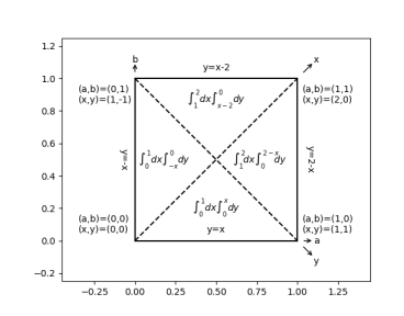
Figure 5: The singularity-aligned coordinate system (98), (99).

The integrals were performed over a non-uniform coordinate-aligned grid in the $(x,y)$ coordinates, using the same non-linear spacing of grid points in each dimension, in an attempt to sample more densely near the singularities. The interval $[0,2]$ was divided by $2n$ cuts, with the $i^{\mbox{\text@underline{\scriptsize th}}}$ cut at

$$1-x_{n-i-1}^{\alpha} \qquad\qquad 0<i<n$$

$$1+x_{i-n}^{\alpha} \qquad\qquad n<i<2n$$ (104)

$$x_{i}=\frac{i+0.5}{n} \qquad\qquad 0\leq i\leq n-1.$$

These cuts define $2n-1$ adjacent 1D cells, each centered at the midpoint of its defining cuts. The function samples were taken at these midpoints. For $0<\alpha<1$, this results in more dense sampling near the ends of the interval than the center. We chose $\alpha=0.5$, somewhat arbitrarily. These intervals were separately rescaled and recentered to cover each of the 4 triangles shown in Figure 5, as well as their reflections through each triangle’s edge along boundary of the domain of integration. Cell centers falling with the domain of integration were counted; the others dropped.

It should not be difficult to improve upon this sampling strategy, perhaps replacing it with something alltogether different such as a Gibbs sampler. The method used should sample fairly accurately near the singularities along the diagonal lines, but neglects to take any special care near the singularities at the external boundaries. In addition to not sampling very densely near the midpoints of those boundaries, no account is taken of the slicing through the sampling rectangles that cross those boundaries. Even so, this was adequate for our present purposes. With $n=1000$, the integral of the non-informative prior came out to 0.9989, so the integrals should be accurate to about 0.1%.

The numerical integration to determine $\kappa(a,b)$ was performed for each $(a,b)$ value by scaling (104) with $n=100,000$ and $\alpha={0.5}$ to the unit interval and accepting those points lying within the integration limits of (30). For the figures, the $(a,b)$ grid was defined with $n=250$. For Figure 2, the numerical integration was performed with $n$ increased to $1,000,000$.