Phase transitions and correlations in fracture processes where disorder and stress compete

Abstract

We study the effect of the competition between disorder and stress enhancement in fracture processes using the local load sharing fiber bundle model, a model that hovers on the border between analytical tractability and numerical accessibility. We implement a disorder distribution with one adjustable parameter. The model undergoes a localization transition as a function of this parameter. We identify an order parameter for this transition and find that the system is in the localized phase over a finite range of values of the parameter bounded by a transition to the non-localized phase on both sides. The transition is first order at the lower transition and second order at the upper transition. The critical exponents characterizing the second order transition are close to those characterizing the percolation transition. We determine the spatiotemporal correlation function in the localized phase. It is characterized by two power laws as in invasion percolation. We find exponents that are consistent with the values found in that problem.

I Introduction

It has been known for a long time that heterogeneities make materials more resilient against failure under load by offsetting the point at which a microfracture becomes unstable wz17 . Examples of materials where heterogeneities play an important role are concrete mhk93 ; ldl19 and carbon-fiber composites ksl08 which possess larger strength and toughness than the individual components l92 ; m93 . Heterogeneities introduce spatial disorder in the local material strength and create spatially dependent dynamic stress field. Under sufficiently large external stress, a micro-crack appears at the weakest point of the material and creates higher stress at the crack tips. Whether this microcrack will grow to a catastrophic failure or different micro-cracks will appear with increasing stress, depends on the dynamic competition between local stress enhancement and local material strength. Therefore, understanding the role of disorder in detail is crucial for technological purposes, in order to optimize the material strength.

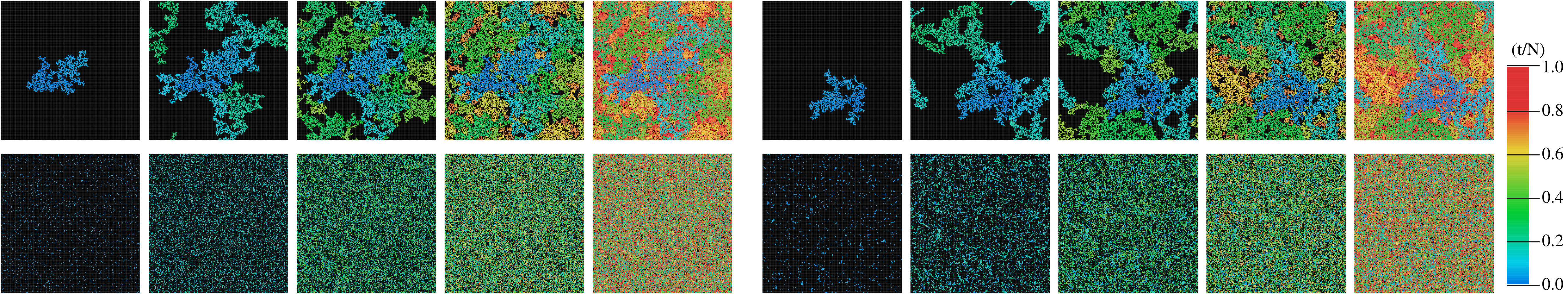
$D>0$ $D<0$

Figure 1: Growth of cracks in a bundle of $256\times 256$ fibers with threshold distribution from Eq. (5). The left and right panels correspond to $D>0$ and $D<0$ respectively. The top and bottom rows in each panel correspond to low ($|D|=0.02$) and high ($|D|=2.0$) disorders respectively. The black sites are intact fibers and the colored sites are broken fibers. The colors represent the breaking sequence ($\tau=t/N$) as indicated by the scale at right. The five snapshots in each set show the evolution of cracks at $\tau=0.04$, $0.2$, $0.4$, $0.6$ and $0.9$.

The interplay between disorder and dynamical effects during the breakdown process of brittle materials was the focus of much research within the statistical physics community during the eighties and nineties hr14 . This research was based on a number of lattice-based models where the links would have a maximum load before they would fail drawn from some spatially uncorrelated distribution. For example the fuse model ahr85 ; dbl86 ; kbrah88 consisted of a network of electrical resistors that would act as fuses, the central force model consisted of a network of freely rotating Hookean springs that would fail if the load they carried crossed a threshold hrh89 , and the beam model hhr89 where the links in the network would be elastic beams that would fail if certain criteria was fulfilled sh19 . We summarize the picture that emerged qualitatively in the following. There are two reasons for a failure to appear locally in a disordered material. Either it is due to the material being weak at that local point or it is due to the stress being high there. Imagine now loading the disordered material. At the beginning of the breakdown process, the material will fail where it is weak as there are no — or few — points with high stress. When local failures develop, spots with intense stress appear at the tips of microcracks. As the failure process proceeds, these high-stress spots will start dominating. As it was argued by Roux and Hansen, rh90 disorder makes local failures repulsive whereas the stress field makes them attractive. Imagine that there is a first local failure. Draw a sphere around this first local failure and identify the weakest spot within the sphere. The larger the sphere is, the weaker the weakest spot within it will be. As a result, if the next local failure is due to the local weakness of the material, it will occur as far as possible from the first one. Hence, the failures are repulsive when they are caused by the disorder in the strength of the material. The effect of the stress field is opposite. The closer one is to a local failure, the higher the largest stress will be. This makes it more likely that the next failure will be close to the one that just appeared. Hence, local failures attract each other when they are due to high stress field. The result of this is that there is a competition between disorder and stress concentration throughout the failure process. Early in the failure process the disorder tends to dominate, resulting in local failures appearing distributed throughout the material. However, as the stress field takes over, there is localization ending with a single growing crack beginning to dominate. Depending on the disorder, localization may occur early or later in the process: The wider the disorder, the later on the onset of localization would occur. In the limit of infinite disorder rhhg88 ; moh12 ; szs13 , localization never sets in and the failure process is a screened percolation — i.e. a process where links fail at random given that they are connected in such a way that they carry stress. When the disorder is weak enough to cause a competition with the stresses, a phase diagram may be constructed showing the onset of localization as a function of the disorder ah89 ; ahhr89 ; hhr91 .

It is the aim of this work to study the effect of the competition between disorder and stress enhancement using the fiber bundle model phc10 ; hhp15 . The advantage of using this model over other models is that it is not computationally demanding, leading to good statistics for large samples. Furthermore, it has a high level of analytical tractability. We describe the fiber bundle model in detail in Sec. II. It should be noted that Stormo et al. sgh12 studied the interplay between disorder and stress enhancement in the soft clamp model which is a more complex version of the fiber bundle model than the version we study here. Their conclusions differ from those we present here; this due to a very different way of analyzing the fracture process. We return to this work in the concluding section. We implement a disorder distribution that has one adjustable parameter. By tuning this parameter, we produce disorders with power law tails towards either zero strength or infinite strength. We focus in Sec. III on the localization transition that occurs for some value of the disorder parameter, see Fig. 2. For the range of the values of the disorder parameter that produces power law tails towards zero strength, we find a second order phase transition, whereas for the range of values for the disorder parameter that produces a power law tail towards infinite strength, we find a first order phase transition. We determine the values of critical exponents associated with the second order phase transition. They are close to those found in percolation. In Sec. IV we study the spatiotemporal correlation function first introduced by Furuberg et al. ffa88 in connection with invasion percolation. We determine the scaling exponents characterizing the correlation function and find them to be close to the values observed for invasion percolation. We relate the exponents to other exponents characterizing the transition using theory developed by Roux and Guyon rg89 , Maslov m95 and Gouyet g90 . We end by drawing our conclusions in Sec. V.

II Description of the Model

The fiber bundle model is a model of fracture where one can control the range of stress enhancement upon the appearance of a crack. In this model, $N$ fibers (Hookean springs) are placed between two clamps under external force $F$. Each fiber carries a force

$$f=\kappa x\;,$$ (1)

where $\kappa$ and $x$ are respectively the elastic constant and extension of the fiber. The extension of each fiber has a threshold ($x_{t}$), beyond which it fails and the load it was carrying is distributed among surviving fibers according to some pre-set rule. The stress distribution scheme models the local stress enhancement whereas the disorder in $x_{t}$ models the local material heterogeneity. If the load of the failed fibers is distributed over all the surviving fibers, there is no local stress enhancement. This is the equal load sharing (ELS) scheme. The ELS fiber bundle model was introduced by Peirce in 1926 p26 as a simple model for failure in fibrous materials. Daniels approached the ELS fiber bundle model as a problem in statistics in a seminal paper in 1945 d45 . If the load is distributed only to the nearby fibers, we are dealing with the local load sharing (LLS) model hp78 ; hp91 . Here local stress enhancement competes with the local heterogeneity leading to localization. Sornette introduced the ELS fiber bundle model to the statistical physics community in 1992 s92 . Soon, the focus of this community was on the rich avalanche statistics that this model offer hh92 ; hh94 ; zd94 ; khh97 , which in the ELS case is analytically tractable.

The sequential — or time — correlation between failure events in the fiber bundle model makes it possible to explore the brittle to ductile transition asl97 within it, a well-studied phenomenon in material science. The spatial correlations between the failures, on the other hand, have not been studied in detail.

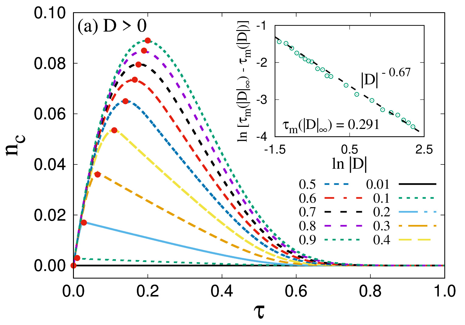
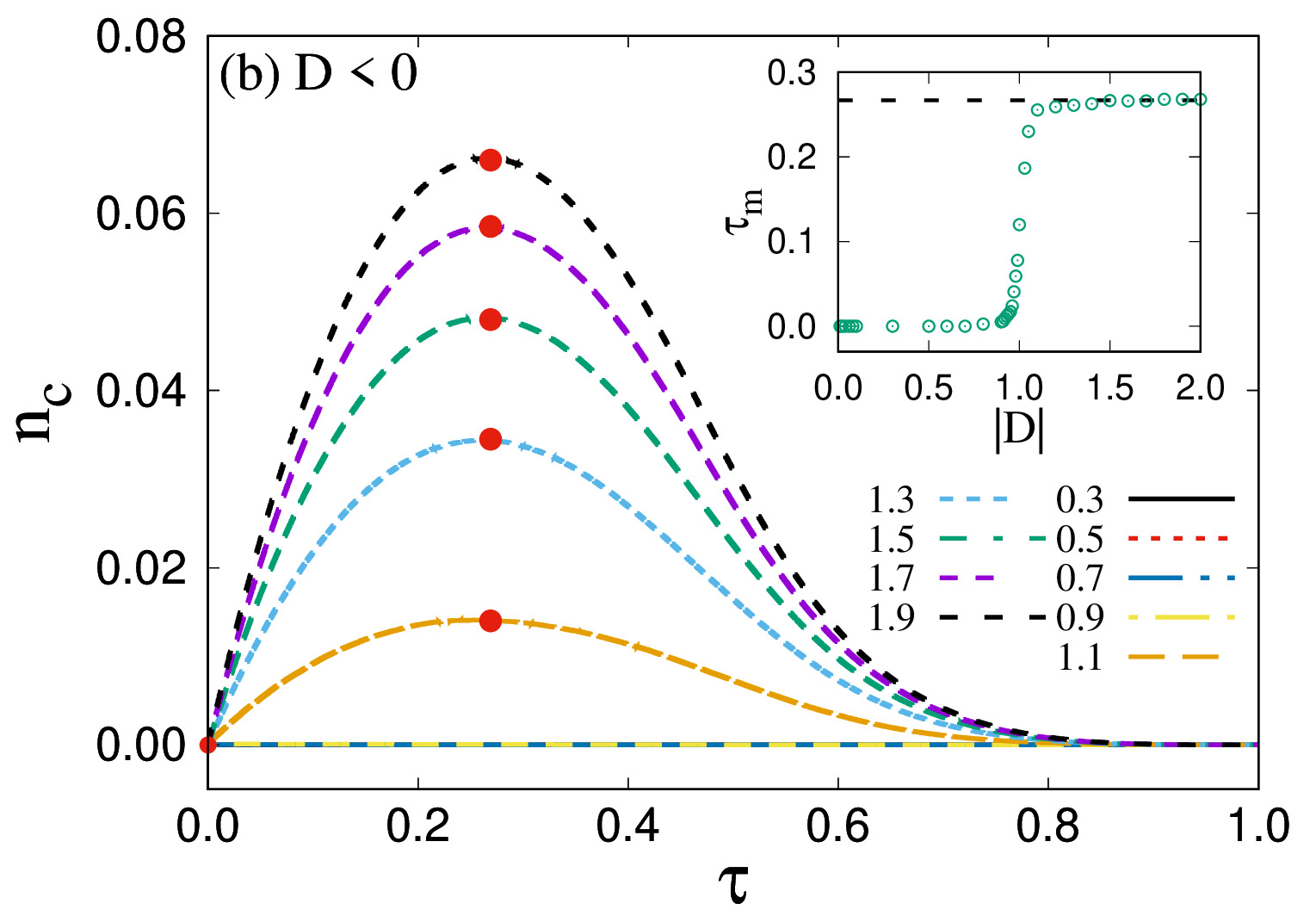
Figure 2: Variation of crack densities $n_{c}$ with fraction of broken bonds $\tau$ for $L=256$ at different disorders. The $|D|$-values are indicated in the legends. The red dots indicate the peaks at ($\tau_{\rm m},n_{c}^{\rm max}$). For $D>0$ we see a gradual increase in $\tau_{\rm m}$ with increasing $|D|$ whereas for $D<0$ we first see a discontinuity from zero to a finite value and then it remains almost constant at $\approx 0.27$. The inset of (a) shows the scaling $\tau_{m}^{+}(|D|_{\infty})-\tau_{m}^{+}(|D|)\sim|D|^{-\gamma}$ for $D>0$ where $\gamma=0.67\pm 0.01$ and $\tau_{m}^{+}(|D|_{\infty})=0.291\pm 0.011$. The inset of (b) shows the convergence of $\tau_{m}^{-}$ towards $|D|\to\infty$ for $D<0$.

In the LLS fiber bundle model, the load carried by the failed fibers is distributed equally among their nearest intact neighbors. We define a crack as a cluster of $s$ failed nearest-neighbor fibers. The perimeter of the crack is the set of $p$ intact fibers that are nearest neighbors to the failed fibers constituting the crack. These nearest neighbors define the hull of the cluster ga87 . The force on an intact fiber $i$ at any instance is then give by

$$f_{i}=\sigma\left(1+\sum_{J(i)}\frac{s_{J(i)}}{p_{J(i)}}\right)\;,$$ (2)

where $\sigma=F/N$, the force per fiber. The summation runs over all cracks $J(i)$ that are neighbors to fiber $i$. This redistribution scheme is independent of the lattice topology and it is also independent of the failure history skh15 , that is, the complete stress field can be calculated from the present arrangement of intact and broken fibers without having to take into account the order in which the fibers failed.

Suppose $t$ fibers have failed. We determine which fiber will fail at time $t+1$ in the following way hhp15 . Let $f_{i}^{1}$ be the force on fiber $i$ if we set the average force on the fibers $\sigma=1$. We then calculate

$$\lambda(t+1)=\max_{i}\left(\frac{f_{i}^{1}}{\kappa x_{t,i}}\right)\;,$$ (3)

which denotes the fiber $j(t+1)$ that fails at time $t+1$. The force $\sigma=\sigma(t+1)$ at which this force fails is given by

$$\sigma(t+1)=\frac{1}{\lambda(t+1)}\;.$$ (4)

The failure thresholds $x_{t}$ of the fibers are assigned by generating a random number over unit interval and raising it to power $D$ which corresponds to the cumulative distribution hhr91 ; sh19

$$P(x_{\rm t})=\begin{cases}x_{\rm t}^{1/|D|}\;,x_{t}\in[0,1]&\text{when}\;D>0\;,\\ 1-x_{\rm t}^{-1/|D|}\;,x_{t}\in[1,\infty)&\text{when}\;D<0\;.\end{cases}$$ (5)

This threshold distribution allows us to control the disorder by the value of $D$, higher value of $|D|$ implies higher disorder. Furthermore, $D>0$ and $D<0$ respectively correspond to the distributions with power law tails towards weaker and stronger fibers, which, as we will see, make the failure dynamics very different.

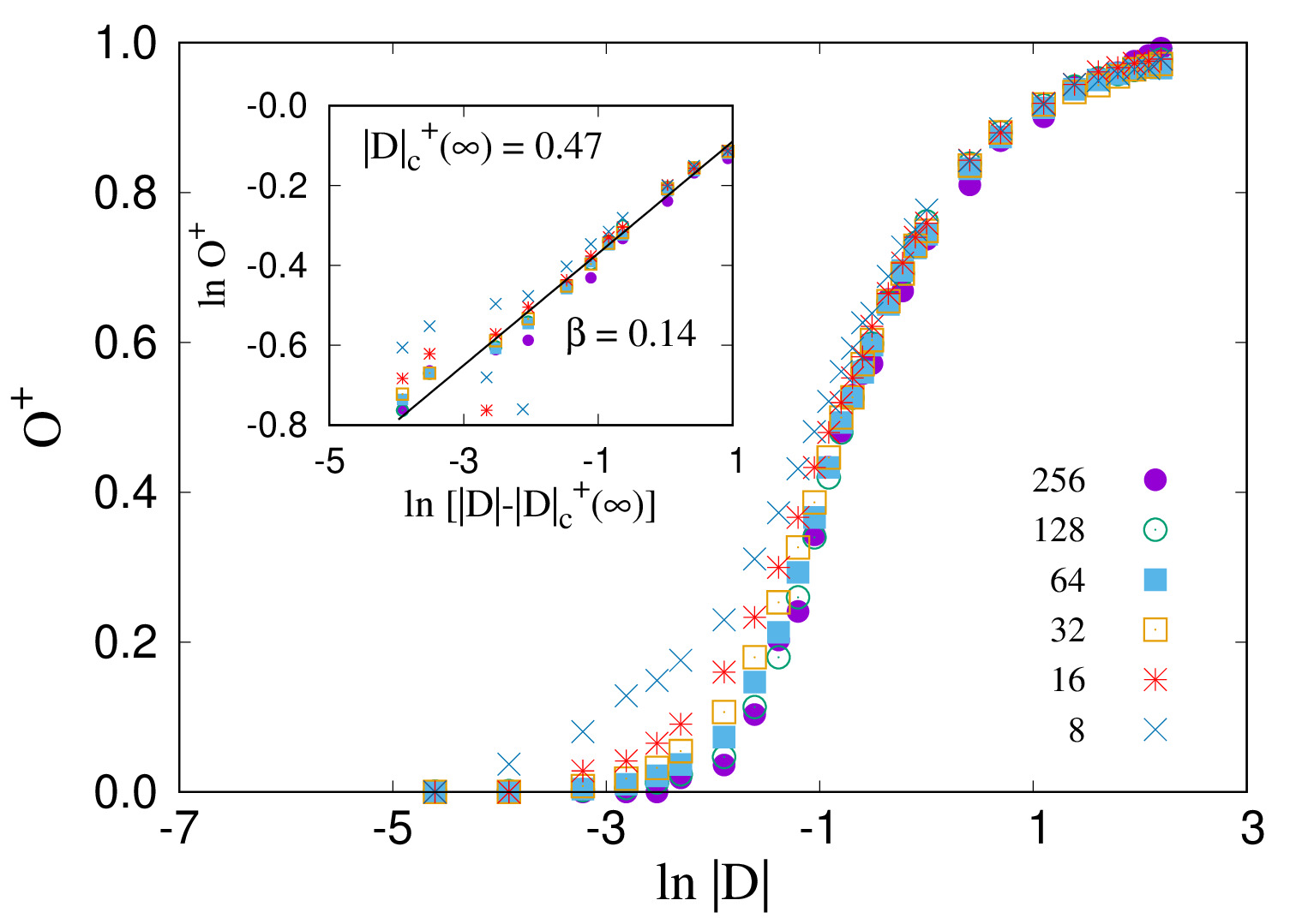
Figure 3: Plot of order parameter $O^{+}$ as a function of disorder $|D|$ for $D>0$. Different symbols indicate different system sizes $L$ where data are averaged over $200$ to $100000$ samples depending on $L$. In the inset, we plot the scaling relation given in Eq. (8) where we find $|D|_{\rm c}^{+}(\infty)=0.47\pm 0.04$ and $\beta=0.14\pm 0.05$.

III Localization Transition

We implement the model on a square lattice of size $N=L\times L$ fibers. The growth of cracks for $L=256$ at different disorders are shown in Fig. 1 where we see two distinct regimes, a single crack growth at low disorder (top row) and random failures at high disorder (bottom row). The color scale in this figure represents where in the breaking sequence a given fiber fails, parameterized by $\tau=t/N$, which we will discuss in detail later. At very low disorder, the stress enhancement at the crack perimeter wins over the fiber strengths and the crack always grows from the perimeter of the existing crack. The local disorder at the perimeter makes the crack grow as an invasion percolation cluster ww83 .

At high disorder, the strength of fibers win over the stress enhancement and we see random clusters of failed fibers appear. These two cases appear to be same for both $D>0$ and $D<0$, however, a completely different picture emerges between these two regimes when we observe crack growth at intermediate disorders. In Fig. 2, we plot the crack density $n_{c}=N_{c}/N$, where $N_{c}$ is the number of cracks (clusters) when $t$ fibers have broken, for different disorders as a function of $\tau=t/N$. We see that $n_{c}$ stays close to $0$ ($N_{c}=1$) for the whole failure process for small $|D|$ values whereas for large $|D|$, $n_{c}$ increases with $\tau$ and reaches a maximum ($n_{c}^{\rm max}$), beyond which, the cracks start to coalesce as more fibers are broken. The position of the peaks at $\tau$-axis, marked by the red dots in Fig. 2, vary continuously with disorder for $D>0$ whereas the peak stays at almost same position for $D<0$ after a discontinuity between the low and high $|D|$ values. Moreover, for two disorders with same values of $n_{c}^{\rm max}$, the peak appears much earlier for $D>0$ compared to $D<0$. This shows that individual cracks appear randomly for $D>0$ whereas cracks grow in size together with the appearance of new cracks for $D<0$. Intuitively, when the threshold distribution has a power-law tail towards strong bonds ($D<0$), probability to find weak bonds at existing crack perimeters are higher, which makes existing cracks to grow. Whereas when power-law tail is towards the weak bonds ($D>0$), probability to find strong bonds at the perimeter is high and new cracks appear at different positions than the perimeter.

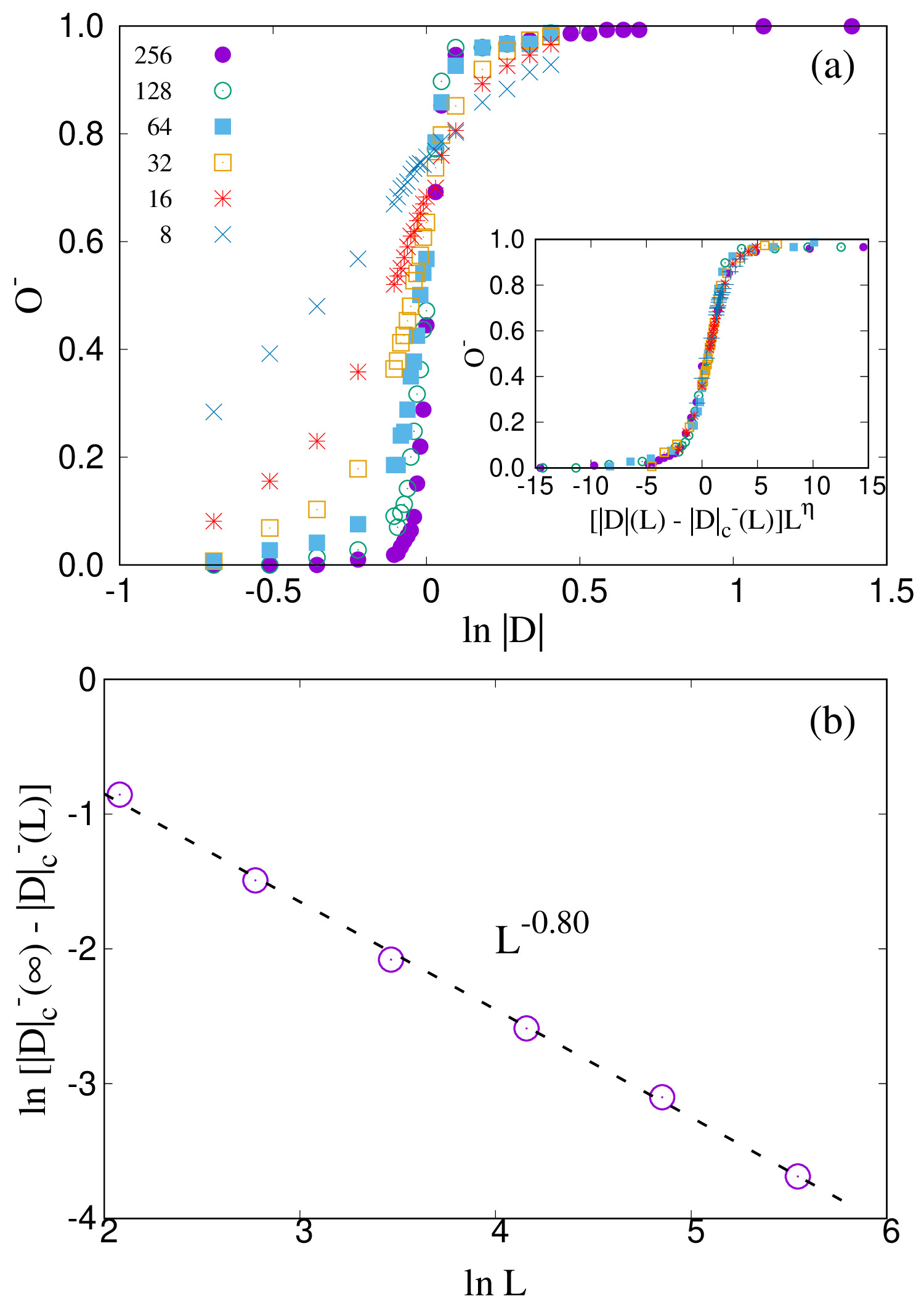
Figure 4: Plot of order parameter $O^{-}$ as a function of disorder for $D<0$ is plotted in (a) which shows abrupt transition with the increase in system size $L$. The inset in (a) shows the scaling with different $L$ according to Eq. (9). In (b), we plot $|D|_{\rm c}^{-}(\infty)-|D|_{\rm c}^{-}(L)\sim L^{-\theta}$ where we find $|D|_{\rm c}^{-}(\infty)=1.03\pm 0.02$ with $\theta=0.80\pm 0.01$.

To characterize this localization transition, we define an order parameter,

$$O^{-/+}(|D|,L)=\frac{\tau_{\rm m}^{-/+}(|D|,L)}{\tau_{\rm m}^{-/+}(|D|_{\infty},L)}$$ (6)

where the plus and minus signs correspond to $D>0$ and $D<0$ respectively. Here $\tau_{\rm m}^{-/+}(|D|,L)$ is the fraction of broken fibers at $n_{c}=n_{c}^{\rm max}$ and $\tau_{\rm m}^{-/+}(|D|_{\infty},L)$ is the value of $\tau_{\rm m}$ for $|D|\to\infty$, i.e., when the breakdown is an uncorrelated percolation process. The measurements of $\tau_{\rm m}^{-/+}(|D|_{\infty},L)$ for $L=256$ are shown in the insets of Fig. 2. For $D>0$ we observe the scaling,

$$\tau^{+}_{\rm m}(|D|_{\infty})-\tau^{+}(|D|)\sim|D|^{-\gamma}\;,$$ (7)

where we have that $\gamma=0.67\pm 0.01$ and $\tau^{+}(|D|_{\infty})=0.291\pm 0.01$. For $D<0$, $\tau_{m}^{-}(|D|)$ converges to a maximum value more abruptly from which we find $\tau^{-}(|D|_{\infty})=0.27$ as shown by the dashed line in the inset.

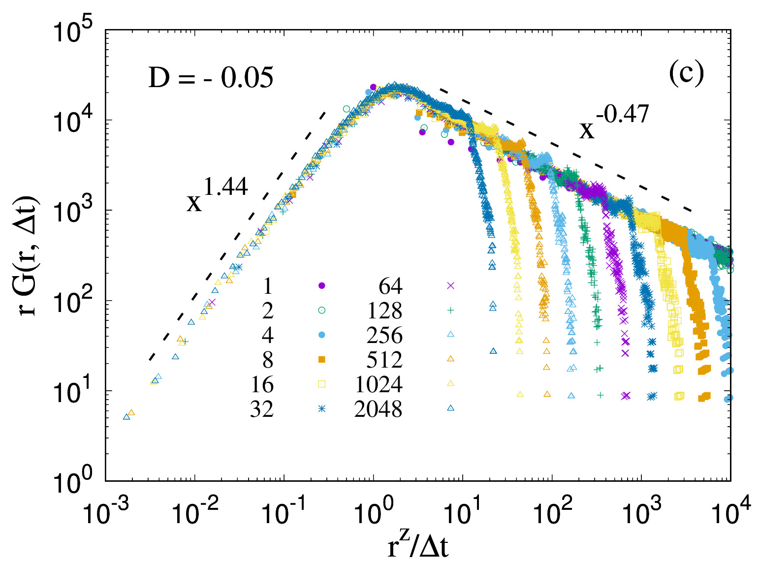
Figure 5: (a) Plot of the largest crack size $s_{\rm max}$ (red symbols) and the largest perimeter size $p_{\rm max}$ (blue symbols) as a function of the system size $L$. From the slopes we find $d_{\rm f}=1.82\pm 0.02$ and $d_{\rm h}=1.74\pm 0.02$. In (b) and (c), we plot the pair correlation function (Eq. (10)) for the $D=+0.05$ and $-0.05$ respectively, where we used $z=d_{\rm f}$ obtained from (a). The different plots correspond to different values of $\Delta t$ as indicated in the figures. From the two power law scalings we find the exponents $a=1.44\pm 0.04$ and $b=0.47\pm 0.06$.

The transition for $D>0$ is explored in Fig. 3, where we plot $O^{+}(|D|,L)$ as a function of disorder for different system sizes. Here $O^{+}$ vary continuously from $1$ to $0$ similar to a second order phase transition. We find the following scaling for $O^{+}$,

$$O^{+}(|D|,L)\sim\left[|D|(L)-|D|_{\rm c}^{+}(\infty)\right]^{\beta}$$ (8)

where $|D|_{\rm c}^{+}(\infty)=0.47\pm 0.04$ and $\beta\approx 0.14\pm 0.05$. The exponent $\beta$ is close to $5/36$, the order parameter exponent for percolation in two dimension n87 ; c87 . However, $1/8$, the exact value from Onsager solution of the two-dimensional Ising model o44 , is also within the precision with which we know $\beta$.

The transition for $D<0$ is presented in Fig. 4 where we plot $O^{-}(|D|,L)$ as a function of disorder. Similar to a first order phase transition, $O^{-}$ shows sharp transition from $0$ to $1$ as the system size $L$ is increased. The plots for different $L$ can be scaled as clb86 ,

$$O^{-}(|D|,L)\sim\Phi\Big{\{}\left[|D|(L)-|D|_{\rm c}^{-}(L)\right]L^{\eta}\Big{\}}$$ (9)

with $\eta=0.7$. This is shown in the inset of Fig. 4(a). The transition disorder $|D|_{\rm c}^{-}(L)$ is observed to be a decreasing function of $L$. To find the value of $|D|_{\rm c}^{-}$ as $L\to\infty$, we use the scaling $|D|_{\rm c}^{-}(\infty)-|D|_{\rm c}^{-}(L)\sim L^{-\theta}$ with $|D|_{\rm c}^{-}(\infty)=1.03\pm 0.02$ and $\theta=0.80\pm 0.01$. This is shown in Fig. 4(b).

IV Spatiotemporal Correlations

We now turn to the investigation of the spatial and temporal correlations during the breakdown process. First we measure the fractal dimension of single cracks at low disorder, defined as $s_{\rm max}\sim L^{d_{\rm f}}$ where $s_{\rm max}$ is size of the largest incipient infinite cluster. This is shown in Fig. 5 (a). We find $d_{\rm f}=1.82\pm 0.02$, and note that this close to the fractal dimension of invasion percolation cluster with trapping ww83 ; lz85 . The colors in Fig. 1 represent the sequence of fiber breaking and together with the positions of broken fibers, they show the spatiotemporal map of the failure process. For random failures at high disorder (bottom row), the pixels (each representing a fiber) of different colors are randomly mixed, whereas for the single crack growth (top row), the different colors are clustered, indicating localization and hence spatial and temporal correlations. To quantify this correlation, we measure pair correlation function $G(r,\Delta t)$, defined as follows: if a fiber at position $\bm{r_{0}}$ breaks at a time $t$, then $G(r,\Delta t)$ provides the probability that another fiber at $\bm{r_{1}}$ will break at time $t+\Delta t$, where $r=|\bm{r_{1}}-\bm{r_{0}}|$. Here time $t$ is measured in terms of the number of broken fibers. This correlation function was first introduced by Furuberg et al. ffa88 for invasion percolation. We assume in the following that the $G(r,\Delta t)$ has the scaling form ffa88

$$G(r,\Delta t)=r^{-1}g\left(\frac{r^{z}}{t}\right)\;,$$ (10)

where $z$ is the dynamic exponent. In Fig. 5, we plot $rG(r,\Delta t)$ for the single crack growth regime as a function of $r^{z}/t$ for $D>0$ (b) and $D<0$ (c). For $z=d_{\rm f}$, the single-parameter function $g$ shows power-law behavior in both the large- and small-argument limits,

$$g(u)\sim\begin{cases}u^{a},&u\ll 1\;\;\textnormal{(long time range)}\;,\\ u^{-b},&u\gg 1\;\;\textnormal{(short time range)\;,}\end{cases}$$ (11)

with a peak at $u=1$ or at $t=r^{d_{\rm f}}$ as shown in the figure. This implies that the most probable growth of the crack after time $t$ occurs at a distance $r^{d_{\rm f}}$, or, the most probable growth at a distance $r$ occurs after a time $t^{1/d_{\rm f}}$. The exponent $a$ in the long time range is found to be $1.44\pm 0.04$ as shown in Fig. 5. This matches with the exponent for invasion percolation dynamics ffa88 . Recently, this scaling was observed experimentally for two-phase flow in porous medium during slow drainage mmf17 with the exponent $a$ ranging between $1.44$ and $1.73$. For the power law in the small-argument limit, we obtain the exponent $b=0.47\pm 0.06$, which is different from $0.68$ obtained by Furuberg et al. for invasion percolation dynamics ffa88 .

The exponents and the errors mentioned above are obtained from the least square fitting of the numerical data. The plots with multiple data file, such as figure 3 inset, figure 5 (b) and (c), the error mentioned is the average of the errors corresponding to individual data.

We may relate the exponents $a$ and $b$ to the exponents controlling the avalanche structure of the failure process following Roux and Guyon rg89 , Maslov m95 and Gouyet g90 . The minimum force applied to the fiber bundle for fiber number $t+1$ to fail is $\sigma(t+1)$ given in Eq. (4). We define a forward avalanche (or burst) of size $\Theta$ starting at time $t$ to be hh92 ; m95

$$\sigma(t+k)<\sigma(t)\ {\rm for}\ k<\Theta\ {\rm and}\ \sigma(t+\Theta)\geq\sigma(t)\;.$$ (12)

A backwards avalanche (or burst) we define as

$$\sigma(t-k)<\sigma(t)\ {\rm for}\ k<\Theta\ {\rm and}\ \sigma(t-\Theta)\geq\sigma(t)\;.$$ (13)

Roux and Guyon rg89 define two distributions, $P_{\Delta t}$ and $Q_{\Theta}(r)$. The first one, $P_{\Delta t}$, gives the distribution of the smallest avalanches $\Theta$ that pass through $\sigma(t)$ and $\sigma(t-\Delta t)$ averaged over $\sigma(t)$. It obeys the power law,

$$P_{\Delta t}(\Theta)\propto\frac{1}{\Delta t}\left(\frac{\Theta}{\Delta t}\right)^{-c_{b}}H(\Theta-\Delta t)\;,$$ (14)

where $H(x)$ is the Heaviside function which is one when $x>0$ and zero otherwise. The second one, $Q_{\Theta}$, gives the distribution of distances between failing fibers within an avalanche of size $\Theta$. Roux and Guyon assume it to follow the power law

$$Q_{\Theta}(r)\propto\frac{1}{\Theta^{1/d_{\rm f}}}\left(\frac{r}{\Theta^{1/d_{\rm f}}}\right)^{\zeta}\;.$$ (15)

The spatiotemporal correlation function $G(r,\Delta t)$ may then be constructed from these two probability distributions,

$$G(r,\Delta t)=\int_{0}^{\infty}P_{\Delta t}(\Theta)Q_{\Theta}(r)d\Theta\;,$$ (16)

which integrates to

$$rG(r,\Delta t)\propto\begin{cases}\left(\frac{r^{d_{\text{f}}}}{\Delta t}\right)^{(1+\zeta)/d_{\text{f}}}&\quad\text{if}\ \ r^{d_{\text{f}}}<\Delta t\;,\\ \left(\frac{r^{d_{\text{f}}}}{\Delta t}\right)^{1-c_{b}}&\quad\text{if}\ \ r^{d_{\text{f}}}>\Delta t\;.\\ \end{cases}$$ (17)

Hence, we have in Eq. (11) that $a=(1+\zeta)/d_{\text{f}}$ and $b=c_{b}-1$. Roux and Guyon suggest $\zeta=d_{\text{f}}-1$ making $a=1$. We propose here that $\zeta=d_{\rm h}$, the fractal dimension of the hull f88 , defined as the set of the sites that are connected to the cluster and at the neighbor to the surroundings. In the LLS fiber bundle model, the stress of a crack is re-distributed to its perimeter, the neighboring unbroken fibers of the crack. In Fig. 5, we plot this largest perimeter size $p_{\rm max}$ with the system size $L$ and from the slope, we find $d_{\rm h}=1.74\pm 0.02$. This value matches with the value of $d_{\rm h}$ for percolation hull, known to be $7/4$ by the relation with $\nu$ by $d_{\rm h}=1+1/\nu$, where $\nu$ is the correlation length exponent which is equal to $4/3$ in two-dimensional percolation srg85 ; rgs86 . Hence, we find that

$$a=\frac{1+d_{\rm h}}{d_{\text{f}}}\;.$$ (18)

With $d_{\text{f}}=1.82\pm 0.02$ and $d_{\rm h}=1.74\pm 0.02$, we find $a=1.51\pm 0.04$, which is close to the observed value.

Maslov m95 related the backwards avalanche exponent $c_{b}$ to the exponent $c_{f}$ that governs the probability to find a forward avalanche of size $\Theta$ when the stress is $\sigma_{0}$ via the expression

$$c_{b}=3-c_{f}\;.$$ (19)

Furthermore, Goyuet in turn related $c_{f}$ to $d_{\rm h}$, $d_{\text{f}}$ and $\nu$,

$$c_{f}=1+\frac{d_{\rm h}-1/\nu}{d_{\rm f}}\;,$$ (20)

so that

$$b=1-\frac{d_{\rm h}-1/\nu}{d_{\rm f}}\;,$$ (21)

which leads $b=0.46$. This is also in accordance with the value we observe, $b=0.47$.

V Conclusion

We have here studied the effect of the competition between disorder and stress enhancement using the local load sharing fiber bundle model. We have done this by varying the disorder using a threshold distribution controlled by a single-parameter $D$. When $D$ is positive, the threshold distribution is a power law towards infinitely weak elements, and when $D$ is negative, the distribution is a power law towards infinitely strong elements. By defining an order parameter distinguishing between the localized and non-localized phases, we find two phase transitions, one at $D=D^{+}_{c}=0.47\pm 0.04$ and one at $D=D^{-}_{c}=-1.03\pm 0.02$. The transition for $D>0$ is second order and the transition for $D<0$ is first order. The second order transition is governed by critical exponents that are consistent with percolation, but also those found for the two-dimensional Ising model. We then studied the spatiotemporal correlation function, finding the same behavior as first seen by Furuberg et al. ffa88 in an invasion percolation context. Some numerical values for the exponents controlling the correlation function are different than found by Furuberg et al., which, by following the scaling analysis of Roux and Guyon rg89 , Maslov m95 and Gouyet g90 , we successfully related to other exponents describing the geometry of the cracks.

The conclusions we present here differ from those that Stormo et al. sgh12 presented. In that work, based on the soft-clamp fiber bundle model, the threshold distribution was the uniform one on the unit interval, i.e. $D=1$. The parameter that was varied, was the elastic constant of the clamps to which the fibers are connected. For a given value of this parameter, the breakdown process would proceed in the beginning as an uncorrelated percolation process up to a certain point at which localization would set in. From this point on, the breakdown process would continue through the growth of a single cluster of broken fibers. This transition would not be a phase transition, but a crossover.

It would be of great interest to repeat the analysis we have presented here using the soft-clamp fiber bundle model. Only then we will be able to distinguish what is model dependent in our conclusions and what is not.

References

- (1) X. Wu and Y. Zhu, Heterogeneous materials: a new class of materials with unprecedented mechanical properties, Mat. Res. Lett. 5, 527 (2017).
- (2) P. J. M. Monteiro, P. R. L. Helene and S. H. Kang, Designing concrete mixtures for strength, elastic modulus and fracture energy, Materials and Structures 26, 443 (1993).
- (3) N. Liang, J. Dai, X. Liu and Z. Zhong, Experimental study on the fracture toughness of concrete reinforced with multi-size polypropylene fibres, Mag. Concr. Res. 71, 468 (2019).
- (4) K. L. Kepple, G. P. Sanborn, P. A. Lacasse, K. M. Gruenberg and W. J. Ready, Improved fracture toughness of carbon fiber composite functionalized with multi walled carbon nanotubes, Carbon 46, 2026 (2008).
- (5) S. M. Lee, Handbook of Composite Reinforcements (Wiley, New York, 1992).
- (6) P. K. Mallick, Fiber-Reinforced Composites: Materials, Manufacturing and Design, 2nd ed. (CRC Press, Boca Raton, FL, 1993).
- (7) H. J. Herrmann and S. Roux, Statistical Models for the Fracture of Disordered Media (Elsevier, Amsterdam, 2014).
- (8) L. de Arcangelis and H. J. Herrmann and S. Redner, A random fuse model for breaking processes, J. Phys. Lett. (France) 46, L585 (1985).
- (9) P. M. Duxbury, P. D. Beale and P. L. Leath, Size Effects of Electrical Breakdown in Quenched random Media, Phys. Rev. Lett. 57, 1052 (1986).
- (10) B. Kahng, G. G. Batrouni, S. Redner, L. de Arcangelis and H. J. Herrmann, Electrical breakdown in a fuse network with random, continuously distributed breaking strengths, Phys. Rev. B 37, 7625 (1988).
- (11) A. Hansen, S. Roux and H. J. Herrmann, Rupture of central-force lattices, J. Phys. France, 50, 733 (1989).
- (12) H. J. Herrmann, A. Hansen and S. Roux, Fracture of disordered, elastic lattices in two dimensions, Phys. Rev. B 39, 637 (1989).
- (13) B. Skjetne and A. Hansen, Implications of Realistic Fracture Criteria on Crack Morphology, Front. Phys. 7, 50 (2019).
- (14) S. Roux and A. Hansen, Early Stages of Rupture of Disordered Materials, Europhys. Lett. 11, 37 (1990).
- (15) S. Roux, A. Hansen, H. J. Herrmann and E. Guyon, Rupture of heterogeneous media in the limit of infinite disorder, J. Stat. Phys. 52, 237 (1988).
- (16) A. A. Moreira, C. L. N. Oliveira, A. Hansen, N. A. M. Araújo, H. J. Herrmann and J. S. Andrade Jr., Fracturing Highly Disordered Materials, Phys. Rev. Lett. 109, 255701 (2012).
- (17) A. Shekhawat, S. Zapperi and J. P. Sethna, From Damage Percolation to Crack Nucleation Through Finite Size Criticality, Phys. Rev. Lett. 110, 185505 (2013).
- (18) L. de Arcangelis and H. J. Herrrmann, Scaling and multiscaling laws in random fuse networks, Phys. Rev. B 39, 2678 (1989).
- (19) L. de Arcangelis, A. Hansen, H. J. Herrmann and S. Roux, Scaling laws in fracture, Phys. Rev. B 40, 877(R) (1989).
- (20) A. Hansen, E. L. Hinrichsen and S. Roux, Scale-invariant disorder in fracture and related breakdown phenomena, Phys. Rev. B 43, 665 (1991).
- (21) S. Pradhan, A. Hansen and B. K. Chakrabarti, Failure processes in elastic fiber bundles, Rev. Mod. Phys. 82, 499 (2010).
- (22) A. Hansen, P. C. Hemmer and S. Pradhan, The Fiber Bundle Model, (Wiley-VCH, Berlin, 2015).
- (23) A. Stormo, K. S. Gjerden and A. Hansen, Onset of localization in heterogeneous interfacial failure, Phys. Rev. E 86, 025101(R) (2012).
- (24) L. Furuberg, J. Feder, A. Aharony and T. Jøssang, Dynamics of Invasion Percolation, Phys. Rev. Lett. 61, 2117.
- (25) S. Roux and E. Guyon, Temporal development of invasion percolation, J. Phys. A: Math. Gen. 22, 3693 (1989).
- (26) S. Maslov, Time Directed Avalanches in Invasion Models, Phys. Rev. Lett. 74, 562 (1995).
- (27) J. F. Gouyet, Invasion noise during drainage in porous media, Physica A 168, 581 (1990).
- (28) F. T. Peirce, 32—X.—Tensile Tests for Cotton Yarns v.—“The Weakest Link” Theorems on the Strength of Long and of Composite Specimens, J. Text. Ind. 17, 355 (1926).
- (29) H. E. Daniels, The statistical theory of the strength of bundles of threads. I, Proc. R. Soc. London Ser. A 183, 405 (1945).
- (30) D. G. Harlow and S. L. Phoenix, The Chain-of-Bundles Probability Model for the Strength of Fibrous Materials II: A Numerical Study of Convergence, J. Compos. Mater. 12, 314 (1978).
- (31) D. G. Harlow and S. L. Phoenix, Approximations for the strength distribution and size effect in an idealized lattice model of material breakdown, J. Mech. Phys. Solids 39, 173 (1991).
- (32) D. Sornette, Mean-field solution of a block-spring model of earthquakes, J. Physique I (France), 2, 2089 (1992).
- (33) P. C. Hemmer and A. Hansen, The Distribution of Simultaneous Fiber Failures in Fiber Bundles, J. Appl. Mech. 59, 909 (1992).
- (34) A. Hansen and P. C. Hemmer, Burst avalanches in bundles of fibers: Local versus global load-sharing, Phys. Lett. A 184, 394 (1994).
- (35) S. D. Zhang and E. J. Ding, Burst-size distribution in fiber-bundles with local load-sharing, Phys. Lett. A 193, 425 (1994).
- (36) M. Kloster, A. Hansen and P. C. Hemmer, Burst avalanches in solvable models of fibrous materials, Phys. Rev. E 56, 2615 (1997).
- (37) J. V. Andersen, D. Sornette and K. T. Leung, Tricritical Behavior in Rupture Induced by Disorder, Phys. Rev. Lett. 78, 2140 (1997).
- (38) T. Grossman and A. Aharony, Accessible external perimeters of percolation clusters, J. Phys. A: Math. Gen. 20, L1193 (1987).
- (39) S. Sinha, J. T. Kjellstadli and A. Hansen, Local load-sharing fiber bundle model in higher dimensions, Phys. Rev. E 92, 020401 (2015).
- (40) D. Wilkinson and J. F. Willemsen, Invasion percolation: a new form of percolation theory, J. Phys. A: Math. Gen. 16, 3365 (1983).
- (41) B. Nienhuis in Phase Transitions and Critical Phenomena, ed. C. Domb, M. Green and J. L. Levowitz, vol. 11 (Academic Press, London, 1987).
- (42) J. L. Cardy in Phase Transitions and Critical Phenomena, ed. C. Domb, M. Green and J. L. Levowitz, vol. 11 (Academic Press, London, 1987).
- (43) L. Onsager, Crystal Statistics. I. A Two-Dimensional Model with an Order-Disorder Transition, Phys. Rev. 65, 117 (1944).
- (44) Murty S. S. Challa, D. P. Landau and K. Binder, Finite-size effects at temperature-driven first-order transitions, Phys. Rev. B. 34, 1841 (1986).
- (45) R. Lenormand and C. Zarcone, Phys. Rev. Lett. 54, 2226 (1985).
- (46) M. Moura, K. J. Måløy, E. G. Flekkøy and R. Toussaint, Invasion Percolation in an Etched Network: Measurement of a Fractal Dimension, Phys. Rev. Lett. 119, 154503 (2017).
- (47) J. Feder, Fractals (Plenum Press and New York and London, 1988).
- (48) B. Sapoval, M. Rosso and J. F. Gouyet, The fractal nature of a diffusion front and the relation to percolation, J. Physique Lett. 46, 149 (1985).
- (49) M. Rosso, J. F. Gouyet and B. Sapoval, Gradient percolation in three dimensions and relation to diffusion fronts, Phys. Rev. Lett. 57, 3195 (1986).