Modulational instability in binary spin-orbit-coupled Bose-Einstein condensates

Abstract

We study modulation instability (MI) of flat states in two-component spin-orbit-coupled (SOC) Bose-Einstein condensates (BECs) in the framework of coupled Gross-Pitaevskii equations for two components of the pseudo-spinor wave function. The analysis is performed for equal densities of the components. Effects of the interaction parameters, Rabi coupling and SOC on the MI are investigated. In particular, the results demonstrates that the SOC strongly alters the commonly known MI (immiscibility) condition, $g_{12}^{2}>g_{1}g_{2}$, for the binary superfluid with coefficients $g_{1,2}$ and $g_{12}$ of the intra- and inter-species repulsive interactions. In fact, the binary BEC is always subject to the MI under the action of the SOC, which implies that ground state of the system is plausibly represented by a striped phase.

I Introduction

Bose-Einstein Condensates (BECs) display a great variety of phenomena which may be efficiently used for simulating diverse effects known in nonlinear optics, condensed matter, and other physical settings simulator . In particular, a lot of interest has been recently drawn to the possibility of implementing artificially engineered spin-orbit coupling (SOC) in the spinor (two-component) BEC Linn ; SOC . SOC interactions, in the Dresselhaus and Rashba Rashba forms, account for a number of fundamental phenomena in semiconductor physics, such as the spin-Hall effect Kato topological superconductivity Hasan , and realization of spintronics spintronics . In solid-state settings, the SOC manifests itself in lifting the degeneracy of single-electron energy levels by linking the spin and orbital degrees of freedom. In the binary BEC, the synthetic SOC may be induced via two-photon Raman transitions which couple two different hyperfine states of the atom. In the first experiment Linn , the pair of states $\left|F=1,m_{F}=0\right\rangle$ and $\left|F=1,m_{F}=-1\right\rangle$ of ⁸⁷Rb atoms were used for this purpose. In the combination with the intrinsic matter-wave nonlinearity, the SOC setting offers a platform for the studies of various patterns and collective excitations in the condensates. These studies address the miscibility-immiscibility transition Gautam and the structure and stability of various nonlinear states, including specific structures of the ground state Stanescu , the Bloch spectrum in optical lattices Hamner , Josephson tunneling Zhang , fragmentation of condensates Song , tricritical points tricrit , striped phases stripes , supercurrents supercurrents , vortices and vortex lattices vortices , solitons, in one- solitons1D , two- solitons2D and three- solitons3D dimensional settings, optical and SOC states at finite temperatures He etc. Effects of SOC in degenerate Fermi gases were considered too fermions .

A fundamental ingredient of the matter-wave dynamics is the modulation instability (MI) of flat (continuous-wave, CW) states against small perturbations initiating the transformation of the constant-amplitude CW into a state with a modulated amplitude profile. The MI, alias the Benjamin-Fier instability BF , is the key mechanism for the formation of soliton trains in diverse physical media, as a result of the interplay between the intrinsic nonlinearity and diffraction/dispersion (or the kinetic-energy term, in terms of the matter-wave dynamics) Agrawal . The nonlinearity in ultracold atomic gases is induced by inter-atomic collisions, which are controlled by the s-wave scattering length. The scattering lengths itself may be controlled by optical Blatt and magnetic Inouye Feshbach resonances, while the SOC strength may be adjusted as a function of the angle between the Raman laser beams, and their intensity Higbie .

The MI in single-component BECs has been addressed in many earlier works Agrawal ; Theochairs ; Salasnich . As in other physical systems BF ; Agrawal , it was concluded that the single-component MI is possible only for the self-focusing (attractive) sign of the nonlinearity Higbie ; Khawaja . In attractive BECs, the formation of soliton trains is initiated by phase fluctuations via the MI Strecker . In two-component BECs, the MI, first considered by Goldstein and Meystre Goldstein , is possible even for repulsive interactions Kasamatsu1 ; Kasamatsu2 , similar to the result known in nonlinear optics Agrawal-XPM , in the case when the XPM (cross–phase-modulation)-mediated repulsion between the components is stronger than the SPM (self-repulsion) of each component. In such a case, the MI creates not trains of bright solitons, but rather domain walls which realize the phase separation in the immiscible binary BEC Poland ; Kasamatsu1 ; Kasamatsu2 ; Ho ; Vidanovic ; Pu ; Robins ; Li1 ; Mithun .

The objective of the present work is the analysis of the MI in the effectively one-dimensional SOC system in the framework of the mean-field approach. This is inspired, in particular, by the recent studies of the dynamical instability of supercurrents, as a consequence of the violation of the Galilean invariance by the SOC in one dimension (1D) supercurrents , 2D instability at finite temperatures He , and phase separation under the action of the SOC Kasamatsu2 ; Gautam . The character of the MI, i.e., the dependence of its gain on the perturbation wavenumber, and the structure of the respective perturbation eigenmodes, determine the character of patterns to be generated by the MI. In particular, one may expect that the MI will lead to the generation of striped structures which realize the ground state in the SOC BEC with the repulsive intrinsic nonlinearity stripes .

The subsequent material is structured as follows. In section II, we present the model based on the system of coupled Gross-Pitaevskii equations (GPEs) for the two-component BEC, including the SOC terms and collisional nonlinearity. In this section, we also derive the dispersion relation for the MI by means of the linear-stability analysis. Results of the systematic analysis of the MI in the binary condensate are summarized in section III. The paper is concluded by section IV.

II The model and modulational-instability (MI) analysis

We take the single-particle Hamiltonian that accounts for the SOC of the combined Dresselhaus-Rashba type, induced by the Raman lasers illuminating the binary BEC. As is known, it can be cast in the form of Linn ; Li ; Cheng

$$\hat{H}_{0}=\frac{{\hat{p}_{x}}^{2}}{2m}+\frac{\hbar k_{L}}{m}{\hat{p}_{x}\sigma_{z}}+\frac{\hbar\Omega}{2}{\sigma_{x}}+V(x),$$ (1)

where ${\hat{p}}_{x}$ is the 1D momentum, $k_{L}$ is the SOC strength, $\Omega$ is the Rabi frequency of the linear mixing, $\sigma_{x,z}$ are the Pauli matrices, and $V(x)$ is the trapping potential. Adding the collisional nonlinear terms, the Hamiltonian produces the system of coupled GPEs for scaled wave functions of the two components, $u_{1,2}=\psi_{1,2}/\sqrt{a}_{\bot}$, where $a_{\perp}\equiv\sqrt{\hbar/(m\omega_{\bot})}$, and $\omega_{\perp}$ is the radius of the transverse confinement which reduces the 3D geometry to 1D Li ; Cheng :

$$i\frac{\partial u_{j}}{\partial t}=-\frac{1}{2}{\frac{\partial^{2}u_{j}}{\partial x^{2}}}+i(-1)^{j}\gamma{\frac{\partial u_{j}}{\partial x}}+\Gamma u_{3-j}+$$

$$(g_{j}|u_{j}|^{2}+g_{12}|u_{3-j}|^{2})u_{j}+V(x)u_{j},~{}j=1,2,$$ (2)

where the length, time, 1D atomic density, and energy are measured in units of $a_{\bot}$, ${\omega_{\bot}}^{-1}$, ${a_{\bot}}^{-1}$ and $\hbar\omega_{\bot}$, respectively. Further, scaled nonlinearity coefficients are $g_{j}={2a_{j}}/{a_{\bot}}$ and $g_{12}={2a_{12}}/{a_{\bot}}$, where $a$ and $a_{12}$ are scattering lengths of the intra- and inter-component atomic collisions. Finally, $\gamma\equiv k_{L}a_{\perp}$ and $\Gamma\equiv{\Omega}/{2\omega_{\bot}}$ are the scaled strengths of the SOC and Rabi coupling, respectively, that may be defined to be positive, except for the situation represented by Fig. 11, see below. The number of atoms in each component is given by $N_{1,2}=\int_{-\infty}^{+\infty}\!|u_{1,2}|^{2}\,\mathrm{d}x$.

In the framework of Eq. (2), we first address the MI of the CW state in the form of a miscible binary condensate with uniform densities $n_{10}$ and $n_{20}$, and a common chemical potential, $\mu$, of both components: $u_{j}=e^{-i\mu t}\sqrt{n_{j0}}$. In the absence of the trapping potential, the densities are determined by algebraic equations Goldstein ; Kasamatsu1 ; Kasamatsu2

$$\Gamma=-{\sqrt{\frac{n_{j0}}{n_{3-j,0}}}(g_{j}n_{j0}+g_{12}n_{3-j,0}-\mu)},~{}j=1,2.$$ (3)

For perturbed wave functions of the form $u_{j}=(\sqrt{n_{j0}}+\delta\psi_{j})e^{-i\mu t}$, linearized equation for the small perturbations are

$$\begin{split}i\frac{\partial\left(\delta\psi_{1}\right)}{\partial t}&=-\frac{1}{2}{\frac{\partial^{2}\left(\delta\psi_{1}\right)}{\partial x^{2}}}-i\gamma{\frac{\partial\left(\delta\psi_{1}\right)}{\partial x}}+\Gamma(\delta\psi_{2}-\sqrt{\frac{n_{20}}{n_{10}}}\delta\psi_{1})\\ \ &+g_{1}n_{10}(\delta\psi_{1}+\delta{\psi_{1}}^{\ast})+g_{12}\sqrt{n_{10}n_{20}}(\delta\psi_{2}+\delta{\psi_{2}^{\ast}}),\end{split}$$ (4)

$$\begin{split}i\frac{\partial\left(\delta\psi_{2}\right)}{\partial t}&=-\frac{1}{2}{\frac{\partial^{2}\left(\delta\psi_{2}\right)}{\partial x^{2}}}+i\gamma{\frac{\partial\left(\delta\psi_{2}\right)}{\partial x}}+\Gamma(\delta\psi_{1}-\sqrt{\frac{n_{10}}{n_{20}}}\delta\psi_{2})\\ &+g_{2}n_{20}(\delta\psi_{2}+\delta{\psi_{2}}^{\ast})+g_{12}\sqrt{n_{10}n_{20}}(\delta\psi_{1}+\delta{\psi_{1}^{\ast}}),\end{split}$$ (5)

where $\ast$ stands for the complex conjugate. We look for eigenmodes of the perturbations in the form of plane waves, $\delta\psi_{j}=\zeta_{j}\cos(kx-\Omega t)+i\eta_{j}\sin(kx-\Omega t)$, with real wavenumber $k$ and, generally, complex eigenfrequency $\Omega$ and amplitudes $\zeta_{j}$, $\eta_{j}$. The substitution of this in Eqs. (LABEL:lin1) and (5) produces the dispersion relation for eigenfrequency $\Omega$:

$$\Omega^{4}+\Omega^{2}\left[-\frac{1}{4}{(k^{2}-2\Gamma)(2k^{2}+G_{1}+G_{2})}-2k^{2}\gamma^{2}-2\Gamma G_{12}\right]$$

$$+\frac{\Omega}{2}\left[k\gamma(k^{2}-2\Gamma)(G_{2}-G_{1})\right]$$

$$+k^{2}\left[\gamma^{2}\left(k^{2}\gamma^{2}+2\Gamma G_{12}-\frac{1}{4}{(k^{2}-2\Gamma)(2k^{2}+G_{1}+G_{2})}\right.\right)$$

$$+\left(\frac{k^{2}}{4}-\Gamma\right)\left.\left(\frac{(k^{2}+G_{1})(k^{2}+G_{2})}{4}-G_{12}^{2}\right)\right]=0,$$ (6)

where we define

$$G_{1}\equiv 4g_{1}n_{10}-2\Gamma,G_{2}\equiv 4g_{2}n_{10}-2\Gamma,~{}G_{12}\equiv 2g_{12}n_{10}+\Gamma.\newline$$ (7)

Quartic equation (6) for $\Omega$ obtained for equal densities of the two components, $n_{10}=n_{20}$ may be simplified to a practically solvable form by assuming that the strengths of the intraspecies interactions are equal, $G_{1}=G_{2}\equiv G$ [in this case, Eq. (3) determines the corresponding chemical potential, $\mu$]. The result is

$${\Omega_{\pm}^{2}}=\frac{1}{2}\left(\Lambda\pm\sqrt{\Lambda^{2}+4R}\right),$$ (8)

where we define

$$\Lambda=2k^{2}\gamma^{2}+\frac{1}{2}{(k^{2}-2\Gamma)(k^{2}+G)}+2\Gamma G_{12},$$ (9)

$$R=(S-\Lambda_{+}\Lambda_{-}),\newline$$ (10)

$$\Lambda_{\pm}=\frac{\Lambda\pm\sqrt{2\Lambda_{1}(\Lambda-\Lambda_{1})}}{2},$$ (11)

$$S=\frac{1}{4}\left\{{(k^{2}-2\Gamma)^{2}}G_{12}^{2}+(G+k^{2})^{2}\Gamma^{2}\right\}$$

$$+\frac{1}{2}\left\{\gamma^{2}k^{2}(G+k^{2})(k^{2}-2\Gamma)\right\},$$ (12)

$$\Lambda_{1}=\frac{1}{2}{(k^{2}-2\Gamma)(G+k^{2})}$$ (13)

The expression given by Eq. (8) may be positive, negative or complex, depending on the signs and magnitudes of the terms involved. The CW state is stable provided that ${\Omega_{\pm}^{2}}>0$ for all real $k$; otherwise, the instability growth rate is defined as $\xi\equiv\left|\text{{Im}}\left(\Omega_{\pm}\right)\right|$. Thus, the MI takes place, with complex ${\Omega_{\pm}^{2}}$, at ${\Lambda}^{2}+4R<0$. At $R>0$, ${\Omega_{+}^{2}}$ is always positive for $\Lambda>0$, hence the CW state is stable against the growth of perturbations accounted for by $\Omega_{+}$. At $\Lambda<0$, ${\Omega_{+}^{2}}$ is negative in the range of $-{\Lambda}^{2}/4\leq R<0$, where the CW state is unstable. Irrespective of the value of $\Lambda$ but for $R>0$, the MI always sets in via the growth of the perturbations which are accounted for by ${\Omega_{-}^{2}<0}$. The commonly known case of the MI in the single-component model, which corresponds to $\gamma=\Gamma=0$, i.e., $G=4g$ and $G_{12}=0$ Agrawal ; Theochairs ; Salasnich , is reproduced by the above results: it occurs for $g<0$ (self-attractive nonlinearity) in the interval of perturbation wavenumbers $0<k<2\sqrt{|g|}$, with the maximum gain, $\xi\equiv\mathrm{Im}\left(\Omega\right)$, attained at $k_{\max}=2\sqrt{g}$.

III Results and discussions

For the experimentally realized SOC system in the condensate of ⁸⁷Rb atoms, equally distributed between the two pseudo-spin states ($n_{10}=n_{20}\equiv n_{0}$; by means of rescaling, we set the common CW density of both components to be $n_{0}=1$), the collisional nonlinearity is repulsive, i.e., $g>0$ and $g_{12}>0$ in Eq. (2). Here, for the sake of generality, we are going to consider the MI in this case, as well as in the system with other signs of the nonlinear terms. Then, depending on the signs of $G$ and $G_{12}$, defined per Eq. (7), four different cases arise. Also, we will compare our results with previously obtained results in absence of SOC.

III.1 MI in the absence of SOC

In the absence of SOC, we here dwell on two special cases, which are $\Gamma=0$ and $\Gamma\neq 0$.

III.1.1 Zero Rabi coupling

For $\Gamma=0$, the model amounts to the usual two-component system, and our solution for $\Omega^{2}$ is

$${\Omega_{\pm}^{2}}=\frac{k^{2}}{2}\left(\frac{k^{2}}{2}+2gn_{10}\pm 2g_{12}n_{10}\right),$$ (14)

which exactly matches the one obtained in Refs. Kasamatsu1 ; Kasamatsu2 . It is well known that, in this case, for repulsive inter- and intra-component interactions, the MI occurs only when $g_{12}^{2}>g_{1}g_{2}$ Mineev . Here it further reduces to $g_{12}>g$.

III.1.2 Non-zero Rabi coupling

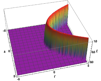
Figure 1: (Color online) The MI gain for $\Omega_{-}$ perturbations at $\gamma=0$. Here $g=2$ and $g_{12}=1$.

In the presence of the Rabi coupling, Eq. 8 is modified as

$${\Omega_{+}^{2}}=\frac{k^{2}}{2}\left(\frac{k^{2}}{2}+2gn_{10}+2g_{12}n_{10}\right),$$ (15)

$${\Omega_{-}^{2}}=\frac{(k^{2}-4\Gamma)}{2}\left(\frac{k^{2}}{2}-2\Gamma+2gn_{10}-2g_{12}n_{10}\right).$$ (16)

The consideration of these solutions shows that $\Omega_{+}$ is real in the following cases: i) both inter- and intra-component interactions are repulsive, ii) attractive inter- and repulsive intra-component interactions, only with $g\geq|g_{12}|$, and iii) repulsive inter- and attractive intra-component interactions, only with $g\leq|g_{12}|$. In other cases, $\Omega_{+}$ is always imaginary. The effect of the Rabi coupling can be seen from expression (16) for $\Omega_{-}$. It is concluded that, whenever $\Gamma$ is negative or zero, $\Omega_{-}$ is real for the cases when i) both inter- and intra-component interactions are repulsive, only with $g\geq|g_{12}|$, ii) attractive inter- and repulsive intra-component interactions, and iii) attractive inter- and intra-component interactions, only with $|g|\leq|g_{12}|$. The situation is similar to that for the case of zero Rabi coupling. The effect of the Rabi coupling becomes appreciable at $\Gamma>0$. Figure 1 shows the MI gain when the strength of the inter-component interaction is smaller than the intra-component strength, and it also shows the gain, $\xi=2\sqrt{(g-g_{12}-\Gamma)\Gamma}$, at $0<\Gamma<(g-g_{12})$. It is seen that the usual MI (immiscibility) condition, $g_{12}>g$ , for the two-component BEC system, with coefficients $g$ and $g_{12}$ of the intra- and inter-species repulsive interactions, is not valid for $\Gamma>0$. On the other hand, when the strengths of the intra- and inter-species repulsive interactions are equal the gain is zero.

III.2 $G>0$ and $G_{12}>0$

This case pertains to the case when both the intra- inter-component modified interactions are repulsive. It follows from Eq. (8) that, for $\Lambda>0$, expressions ${\Omega_{\pm}}$ are complex at ${\Lambda}^{2}+4R<0$. This corresponds to a single unstable region on the axis of the perturbation wavenumber, $k$, as shown in Fig 2.

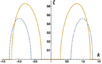
Figure 2: (Color online) The gain of the MI against $\Omega_{+}$ perturbations for $\gamma=\Gamma=1$. The solid line: $G=4~{}(g=1.5)$ and $G_{12}=3~{}(g_{12}=1)$. The dashed line: $G=2~{}(g=1)$ and $G_{12}=3~{}(g_{12}=1)$.

On the other hand, Eq. (8) yields an unstable $\Omega_{-}$ branch at ${\Lambda}^{2}+4R>0$ too. Two instability regions of $k$, corresponding to this branch, are obtained, as shown in Fig. 3, for small values of the interactions coefficient $G$ [see Eq. (7)], while the increase of $G$ leads to merger of the two regions into one, as seen in Fig. 4, which shows the variation of the MI gain, $\xi$, and the range of the values of wavenumber $k$ in which the MI holds, with the variation of $G$ and $G_{12}$. For smaller values of $G_{12}$ at fixed $G>0$, the MI gain in the inner instability band gradually decreases to zero, while the gain in the outer band at first vanishes, and then starts to grow with the growth of $G_{12}$, as shown in Fig. 5. The increase in $G_{12}$ than $G$ makes term ${\Lambda}^{2}+4R$ positive, hence the MI occurs only at $\sqrt{{\Lambda}^{2}+4R}>0<\Lambda$, which shifts the gain band outwards. A general conclusion of the above analysis is that, while, in the case of $0<g_{12}<g$, the usual system of the coupled GPEs does not give rise to the MI, the inclusion of the SOC terms makes all the symmetric ($n_{10}=n_{20}$) CW states, including those with $0<G_{12}<G$, modulationally unstable.

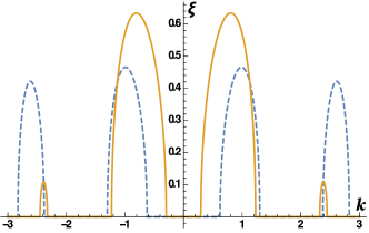
Figure 3: (Color online) The MI gain corresponding to the $\Omega_{-}$ perturbation branch for $\gamma=\Gamma=1$. The solid line: $G=4~{}(g=1.5)$ and $G_{12}=3~{}(g_{12}=1)$. The dashed line: $G=2~{}(g=1)$ and $G_{12}=3~{}(g_{12}=1)$.

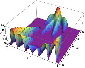
Figure 4: (Color online) The change of the MI gain with the variation of $G$ for fixed $G_{12}=3$ ($g_{12}=1$). Note that $G$ takes both positive and negative values. Here $\gamma=\Gamma=1$.

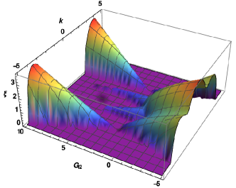
Figure 5: (Color online) The change of the MI gain with the the variation of $G_{12}$ for fixed $G=2$ ($g=1$). Note that $G_{12}$ takes both positive and negative values. Here $\gamma=\Gamma=1$.

III.3 $G<0$ and $G_{12}>0$

This situation refers to the binary BEC with attractive intra-component and repulsive inter-component interactions, which is subject to the MI in the absence of the SOC, although the SOC may essentially affect the instability. Here ${\Omega_{+}}$ produces the same number of MI bands as in the previous subsection, while $\Omega_{-}$ produces more bands. For the $\Omega_{-}$ branch, the largest MI gain in the inner band is always smaller than in the outer one, both increasing with the growth of $G$ at fixed $G_{12}$, as shown in Fig. 4, while the MI gain in the inner MI band decreases to zero, and increases in the outer band with the growth of $G_{12}$ at fixed $G$, as in previous case, as shown in Fig. 6.

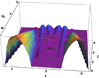
Figure 6: (Color online) The change of the MI gain with variation of $G_{12}$ at fixed $G=-6$ ($g=-1$). Here $\gamma=\Gamma=1$.

III.4 $G>0$ and $G_{12}<0$

In this case, the inter-component interaction is attractive, while the intra-component nonlinearity is self-repulsive, and the MI of the CW with equal densities of both components occurs provided that $\left|g_{12}\right|>g$, in the absence of the SOC and Rabi coupling, while the latter condition is not relevant for $\Gamma>0$ with $\gamma=0$, see Eq. (16). If the SOC terms are included, a single MI region is generated by both $\Omega_{-}$ and $\Omega_{+}$ perturbation branches. This is possible only for ${\Lambda}^{2}+4R>0$ with $\Lambda<0$. The MI accounted for by $\Omega_{-}$ occurs in the range of $0\leq k<\sqrt{\beta+2\beta_{1}+\sqrt{\beta^{2}+4\beta\beta_{2}+4\beta_{1}^{2}}}$, where $\beta\equiv(2|G_{12}|-G)/2$, $\beta_{1}\equiv\gamma^{2}+\Gamma$, $\beta_{2}\equiv\gamma^{2}-\Gamma$, and the largest MI gain, $\xi_{\max}=\sqrt{\Gamma(2|G_{12}|+G)}$, corresponds to $k=0$, as shown in Fig. 7.

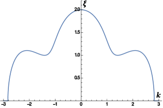
Figure 7: (Color online) The MI corresponding to the $\Omega_{-}$ perturbation branch with $\gamma=\Gamma=1$, $G=2~{}(g=1)$ and $G_{12}=-1$ $(g_{12}=-1)$.

For a fixed value of $G$, which in this case is positive, local maxima of the MI gain, $\xi$ (other than at $k=0$), gradually evolve with the growth of $G_{12}$, resulting in diminished gain at $k=0$, as shown in Fig. 8.

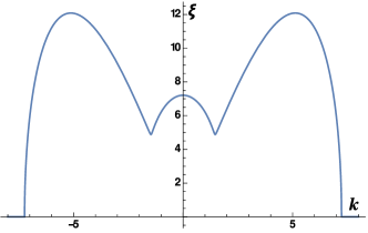
Figure 8: (Color online) The MI corresponding to the $\Omega_{-}$ perturbation branch with $\gamma=\Gamma=1$, $G=2$ $(g=1)$ and $G_{12}=-25$ $(g_{12}=-13)$.

III.5 $G<0$ and $G_{12}<0$

When both the intra- and inter-component interactions are attractive, multiple MI bands are, quite naturally, formed for small values of $G_{12}$ at fixed $G<0$. They ultimately merge into a single band around $k=0$, as shown in Fig. 9. In Figs. 8 and 9, it is seen that, with the growth of $G_{12}$, the situation for the present case effectively simplifies into that reported in the previous subsection, implying that the MI becomes independent of the nature of the intra-component interaction for the strong inter-component attraction.

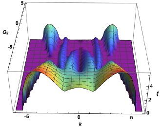
Figure 9: (Color online) The change of the MI gain with the variation of $G_{12}$ for fixed $G=-6$ ($g=-1$).

III.6 Effect of the spin-orbit-coupling on the modulational instability

The above results display the MI gain as a function of the modified nonlinearity coefficients, $G$ and $G_{12}$, at fixed values of the SOC parameters, $\gamma$ and $\Gamma$. It is relevant too to display the gain as a function of the latter parameters, for a fixed strength of the nonlinearity. To this end, Fig. 11 shows the MI gain versus $\gamma$ and $\Gamma$, for fixed $G$ and $G_{12}$. The fixed value of the perturbation wavenumber, $k=1$, is chosen from Fig. 3, where the gain’s maximum is observed for $G=2$ and $G_{12}=3$ at $k=1$.

As mentioned above, it is commonly known that, in the two-component repulsive condensates, the MI, leading to the immiscibility of the binary superfluid, occurs in the region of $g_{12}^{2}>g_{1}g_{2}$ (if the self-repulsion coefficients are different in the two components, $g_{1}\neq g_{2})$ Mineev ; Timmermans ; Kasamatsu1 ; Kasamatsu2 . On the other hand, it was more recently demonstrated that the linear interconversion between the components (accounted for by coefficient $\Gamma$ in the present notation) shifts the miscibility threshold to larger values of $g_{12}$ Merhasin . In the presence of the SOC, Figs. 2 and 3 clearly show that the MI also occurs at $g_{12}\leq g$, for $g_{1}=g_{2}$ and equal CW densities in the two components.

In the latter connection, it is relevant to mention that, for the fixed values $G=2$ and $G_{12}=3$, and setting $\gamma=0$ (no SOC proper, while the Rabi mixing is present, $\Gamma\neq 0$), the MI condition, $g_{12}>g$, holds in the range of $|\Gamma|<1$. Figure 11 shows that the MI is indeed present in this range at $\gamma=0$. On the other hand, the same figure shows zero MI gain for $g_{12}\leq g$ and $\gamma=0$. This observation elucidates the validity of our analysis. In order to see the effect of $\gamma$, we increase the strength of intra-component interaction to $G=10$. For this value, condition $g_{12}<g$ holds for the region of $-1<\Gamma<3$. Figure 11 shows that the MI gain does not vanish in this region. This shows that, in presence of the SOC, irrespective of the sign of the Rabi coupling, the system with repulsive interactions is always subject to the MI.

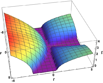
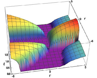
Figure 10: (Color online) The MI gain corresponding to the $\Omega_{-}$ perturbation branch for $G=2$,$G_{12}=3$ and $k=1$, as a function of the SOC coefficient, $\gamma$ and $\Gamma$.

Figure 11: (Color online) The MI gain corresponding to the $\Omega_{-}$ perturbation branch for $G=10$, $G_{12}=3$, and $k=2$, as a function the SOC coefficients, $\gamma$ and $\Gamma$,

The results of the analysis of the MI are summarized in Table I.

Table 1: Summary of results the MI analysis obtained for different combination of the parameters.

Cases	$\gamma$	$\Gamma$	$G$	$G_{12}$	Inference
1	0	0	+	0	Always Stable
			-		Always unstable
2	0	0	+	+	Unstable only if $g_{12}>g$
			+	-	Unstable only if $|g_{12}|>g$
			-	+	Always unstable
			-	-
3	0	$\neq 0$	+	+	For $\Gamma>0$, always unstable, except for the case of $g=g_{12}$ when both $G$ and $G_{12}$ are positive, and miscibility condition $g_{12}>g$ is invalid. For $\Gamma\leq 0$, this special case reduces to case 2
			+	-
			-	+
			-	-
4	$\neq 0$	$\neq 0$	+	+	The binary BEC is always vulnerable to the MI, irrespective of the nature of the nonlinear interactions
			+	-
			-	+
			-	-

IV Conclusions

We have considered the modulational instability (MI) of the flat CW background with equal densities of two components in the nonlinear BEC, subject to the action of the spin-orbit coupling (SOC). This was done by means of the linear-stability analysis for small perturbations added to the CW states. The SOC acting on the binary BEC affects the phase separation or mixing between the components, driven by the competition of intra- and inter-component interactions. The effective modification induced by the SOC is different for these interactions, the former and latter interactions being, respectively, reduced and enhanced by the Rabi coupling [measured by coefficient $\Gamma$ in Eq. (2)]. Our analysis shows that, irrespective of the sign of inter and intra-component interactions, the system is vulnerable to the MI. For the fixed strength of $\gamma$ and $\Gamma$, the MI becomes independent of the nature of the intra-component interactions when the inter-component attraction is strong. The main result of our analysis is the strong change of the commonly known phase-separation condition $g_{12}^{2}>g_{1}g_{2}$ for the binary superfluid with repulsive interactions.

It may be expected that the nonlinear development of the MI will lead to establishment of multidomain patterns, such as the above-mentioned striped ones (see, e.g., Ref. stripes ). Systematic numerical analysis of such scenarios will be reported elsewhere.

V Acknowledgements

K.P. thanks agencies DST, CSIR, NBHM, IFCPAR and DST-FCT, funded by the Government of India, for the financial support through major projects.

References

- (1) P. Hauke, F. M. Cucchietti, L. Tagliacozzo, I. Deutsch, and M. Lewenstein, Rep. Prog. Phys. 75, 082401 (2012).
- (2) Y. J. Lin, K. Jimenez-Garcia, and I. B. Spielman, Nature (London) 471, 83(2011).
- (3) J. Dalibard, F. Gerbier, G. Jūzeliunas, and P. Öhberg, Rev. Mod. Phys. 83, 1523 (2011); I. B. Spielman, Ann. Rev. Cold At. Mol. 1, 145 (2012); H. Zhai, Int. J. Mod. Phys. B 26, 1230001 (2012); V. Galitski and I. B. Spielman, Nature 494, 49 (2013); X. Zhou, Y. Li, Z. Cai, and C. Wu, J. Phys. B: At. Mol. Opt. Phys. 46, 134001 (2013); N. Goldman, G. Jūzeliunas, P. Öhberg, and I. B. Spielman, Rep. Progr. Phys. 77, 126401 (2014).
- (4) G. Dresselhaus, Phys. Rev. 100, 580 (1955); Y. A. Bychkov and E. I. Rashba, J. Phys. C 17, 6039 (1984).
- (5) Y. K. Kato, R. C. Myers, A. C. Gossard, and D. D. Awschalom, Science 306, 1910 (2004).
- (6) M. Z. Hasan and C. L. Kane, Rev. Mod. Phys. 82, 3045 (2010).
- (7) I. Žutić, J. Fabian, and S. Das Sarma, Rev. Mod. Phys. 76, 323 (2004); C. H. L. Quay, T. L. Hughes, J. A. Sulpizio, L. N. Pfeiffer, K. W. Baldwin, K. W. West, D. Goldhaber-Gordon, and R. de Picciotto, Nature Phys. 6, 336 (2010).
- (8) S. Gautam and S. K. Adhikari, Phys. Rev. A 90, 043619 (2014).
- (9) T. D. Stanescu, B. Anderson, and V. Galitski, Phys. Rev. A 78, 023616 (2008); S. Gopalakrishnan, A. Lamacraft, and P. M. Goldbart, Phys. Rev. A 84, 061604(R) (2011); M. Merkl, A. Jacob, F. E. Zimmer, P. Öhberg, and L. Santos, Phys. Rev. Lett. 104, 073603 (2010).
- (10) C. Hamner, Y. Zhang, M. A. Khamehchi, M. J. Davis, and P. Engels, Phys. Rev. Lett. 114, 070401 (2015); Y. Zhang, and C. Zhang, Phys. Rev. A 87, 023611 (2013).
- (11) D. W. Zhang, L. B. Fu, Z. D. Wang, and S.-L. Zhu, Phys. Rev. A 85, 043609 (2012).
- (12) S. W. Song, Y. C. Zhang, H. Zhao, X. Wang, and W. M. Liu, Phys. Rev. A 89, 063613 (2014).
- (13) Y. Li, L. P. Pitaevskii, and S. Stringari, Phys. Rev. Lett. 108, 225301 (2012).
- (14) C. Wang, C. Gao, C. M. Jian, and H. Zhai, Phys. Rev. Lett. 105, 160403 (2010); D. A. Zezyulin, R. Driben, V. V. Konotop, and B. A. Malomed, Phys. Rev. A 88, 013607 (2013).
- (15) T. Ozawa, L. P. Pitaevskii and S. Stringari, Phys. Rev. A 87, 063610 (2013).
- (16) B. Ramachandhran, B. Opanchuk, X.-J. Liu, H. Pu, P. D. Drummond, and H. Hu, Phys. Rev. A 85, 023606 (2012); H. Sakaguchi and B. Li, ibid. 87, 015602 (2013); Y. Xu, Y. Zhang, and B. Wu, ibid. 87, 013614 (2013); A. L. Fetter, ibid. 89, 023629 (2014) ; P. Nikolić, ibid. 90, 023623 (2014).
- (17) V. Achilleos, D. J. Frantzeskakis, P. G. Kevrekidis, and D. E. Pelinovsky, Phys. Rev. Lett. 110, 264101 (2013); Y. V. Kartashov, V. V. Konotop, and F. K. Abdullaev, Phys. Rev. Lett. 111, 060402 (2013); Y. Xu, Y. Zhang, and B. Wu, Phys. Rev. A 87, 013614 (2013); L. Salasnich and B. A. Malomed, ibid. 87 063625 (2013); Y.-K. Liu and S.-J. Yang, EPL 108, 30004 (2014); Y. Cheng, G. Tang, and S. K. Adhikari, Phys. Rev. A 89, 063602 (2014); Y. V. Kartashov, V. V. Konotop, and D. A. Zezyulin, ibid. 90, 063621 (2014); Y. Zhang, Y. Xu, and T. Busch, ibid. 91, 043629 (2015); P. Beličev, G. Gligorić, J. Petrović, A. Maluckov, L. Hadžievski, and B. Malomed, J. Phys. B: At. Mol. Opt. Phys. 48, 065301 (2015); M. Salerno and F. Kh. Abdullaev, Phys. Lett. A 379, 2252 (2015); S. Gautam and S. K. Adhikari, Phys. Rev. A 91, 063617 (2015).
- (18) H. Sakaguchi, B. Li, and B. A. Malomed, Phys. Rev. E 89, 032920 (2014); H. Sakaguchi and B. A. Malomed, ibid. 90, 062922 (2014); V. E. Lobanov, Y. V. Kartashov, and V. V. Konotop, Phys. Rev. Lett. 112, 180403 (2014); L. Salasnich, W. B. Cardoso, and B. A. Malomed, Phys. Rev. A 90, 033629 (2014); Y. Xu, Y. Zhang, and C. Zhang, ibid. 92, 013633 (2015).
- (19) Y. -C. Zhang, Z. -W. Zhou. B. A. Malomed, and H. Pu, arXiv:1509.04087.
- (20) P. S. He, J. Zhao, A. C. Geng, D. H. Xu, R. Hu, Phys. Lett. A 377, 2207 (2013).
- (21) P. Wang, Z. Q. Yu, Z. Fu, J. Miao, L. Huang, S. Chai, H. Zhai, and J. Zhang, Phys. Rev. Lett. 109, 095301 (2012); L. W. Cheuk, A. T. Sommer, Z. Hadžibabić, T. Yefsah, W. S. Bakr, and M. W. Zwierlein, ibid. 109, 095302 (2012).
- (22) T. B. Benjamin and J. E. Feir, J. Fluid Mech. 27, 417 (1967)
- (23) S. Blatt, T. L. Nicholson, B. J. Bloom, J. R. Williams, J. W. Thomsen, P. S. Julienne, and J. Ye, Phys. Rev. Lett. 107, 073202 (2011); M. Theis, G. Thalhammer, K. Winkler, M. Hellwig, G. Ruff, R. Grimm, and J. H. Denschlag, ibid. 93, 123001 (2004); M. Yan, B. J. DeSalvo, B. Ramachandhran, H. Pu, and T. C. Killian, ibid. 110, 123201 (2013).
- (24) S. Inouye, M. R. Andrews, J. Stenger, H.-J. Miesner, D. M. Stamper-Kurn, and W. Ketterle, Nature (London) 392, 151 (1998); S. L. Cornish, N. R. Claussen, J. L. Roberts, E. A. Cornell, and C. E. Wieman, Phys. Rev. Lett. 85, 1795 (2000).
- (25) J. Higbie, and D. M. Stamper-Kurn, Phys. Rev. Lett. 88, 090401(2002).
- (26) G. P. Agrawal, Non-linear Fiber Optics, 5th ed. (San Diego: Academic, 2013).
- (27) U. Al Khawaja, H. T. C. Stoof, R. G. Hulet, K. E. Strecker, and G. B. Partridge, Phys. Rev. Lett. 89, 200404 (2002).
- (28) G. Theocharis, Z. Rapti, P. G. Kevrekidis, D. J. Frantzeskakis, and V. V. Konotop, Phys. Rev. A 67, 063610 (2003)
- (29) L. Salasnich, A. Parola, and L. Reatto, Phys. Rev. Lett. 91, 080405 (2003).
- (30) K. E. Strecker, G. B, Partridge, A. G. Truscott, and R. G. Hulet, Nature (London) 417, 150 (2002); L. D. Carr and J. Brand, Phys. Rev. Lett. 92 040401 (2004); U. Al Khawaja, H. T. C. Stoof, R. G. Hulet, K. E. Strecker, and G. B. Partridge, Phys. Rev. Lett. 89 200404 (2002).
- (31) E. V. Goldstein, and P. Meystre, Phys. Rev. A 55, 2935 (1997).
- (32) K. Kasamatsu, and M. Tsubota, Phys. Rev. Lett. 93, 100402 (2004).
- (33) K. Kasamatsu, and M. Tsubota, Phys. Rev. A 74, 013617 (2006).
- (34) M. Yu, C. J. McKinstrie, and G. P. Agrawal, Phys. Rev. E 48, 2178-2186 (1993).
- (35) M. Trippenbach, K. Goral, K. Rzazewski, B. Malomed, and Y. B. Band, J. Phys. B: At. Mol. Opt. 33, 4017 (2000).
- (36) T.-L. Ho and V. B. Shenoy Phys. Rev. Lett. 77. 3276 (1996)
- (37) I. Vidanović, N. J. V. Druten and M. Haque, New J. Phys. 15, 035008 (2013)
- (38) H. Pu, C. K. Law, S. Raghavan, J. H. Eberly, and N. P. Bigelow, Phys. Rev. A 60, 1463 (1999).
- (39) N. P. Robins, W. Zhang, E. A. Ostrovskaya, and Y. S. Kivshar, Phys. Rev. A 64, 021601 (2001).
- (40) L. Li, Z. Li, B. A. Malomed, D. Mihalache, and W. M. Liu, Phys. Rev. A 72, 033611 (2005).
- (41) T. Mithun and K. Porsezian, Phys. Rev. A 85, 013616 (2012).
- (42) Y. Li, G. I. Martone, L. P. Pitaevskii, and S. Stringari, Phys. Rev. Lett. 110, 235302 (2013); L. Salasnich and B. A. Malomed, Phys. Rev. A 87, 063625 (2013).
- (43) Y. Cheng, G. Tang, S. K. Adhikari, Phys. Rev. A, 89, 063602 (2014).
- (44) V. P. Mineev, Zh. Eksp. Teor. Fiz. 67, 263 (1974) [Sov. Phys. JETP 40, 132 (1974)].
- (45) M. I. Merhasin, B. A. Malomed, and R. Driben, J. Phys. B: At. Mol. Opt. Phys. 38, 877 (2005).
- (46) E. Timmermans, Phys. Rev. Lett. 81, 5718 (1998).