$p$-order Tensor Products with Invertible Linear Transforms

Abstract

This paper studies the issues about tensors. Three typical kinds of tensor decomposition are mentioned. Among these decompositions, the t-SVD is proposed in this decade. Different definitions of rank derive from tensor decompositions. Based on the research about higher order tensor t-product and tensor products with invertible transform, this paper introduces a product performing higher order tensor products with invertible transform, which is the most generalized case so far. Also, a few properties are proven. Because the optimization model of low-rank recovery often uses the nuclear norm, the paper tries to generalize the nuclear norm and proves its relation to multi-rank of tensors. The theorem paves the way for low-rank recovery of higher order tensors in the future.

1 Introduction

Nowadays, tensor-valued high dimensional data can be often observed in many areas, such as seismic data [4],hyperspectral image [2], and video de-noising [21]. Matrix-based methods may damage the inherent structure of data and hide some connection inside data by vectorizing or matricizing. So it is necessary for us to do research about tensors. There are three typical kinds of tensor decompositions, i.e., CP [6, 9], Tucker decomposition [19, 13] and t-SVD [11]. We refer the readers to [12] for a thorough review of CP and Tucker decomposition. The rank derived by CP decomposition is NP hard to compute [5]. Tucker decomposition may not give the best approximation of tensors. In this decade, there is a new tensor product called t-product [11]. Most of conclusions in the matrix case can be generalized to tensors using this product. We can derive a generalized matrix SVD in the case of tensor based on t-product. Authors in [10] analyzed this product in an operator perspective and proposed more concepts in a generalized version. A special case of $p$-order tensors ($p>3$) product is given [16].They mainly use the concept of matrix slices. The generalized t-product is given for the third order tensor based on any invertible transform [8]. Now we see many applications of this product [4, 2, 7]. This is the most natural kind of product corresponding to matrix cases. In this paper, I generalized this product to the case of $p$-order tensors with invertible linear transforms. To the best of my knowledge, this is the most generalized case explicitly presented so far. Moreover, different definitions of tensor ranks, derived from tensor decompositions, facilitate the research about low-rank recovery. The nature of low-rank means that data such as images,videos, texts, all lie on low-dimensional subspaces [1, 3]. In the matrix case, there are many efficient methods about low-rank recovery like [14]. Among these methods, convex programming with the matrix nuclear norm is very popular. I summarize the main contribution of the paper as follows,

$\bullet$ I propose a $p$-order tensor product using linear invertible transforms.I extend and generalize the work [8, 16]. I also give some related definitions and prove some properties.

$\bullet$ I give a definition of $p$-order tensor nuclear norm and prove a theorem to show the reasonableness of this norm, which is a generalization of [18].We can use it to do research about $p$-order tensor low-rank recovery in the future.

1.1 Notation

In this paper, the vector is denoted like $\mathbf{a}$ and its $i$-th element is like $a_{i}$. A matrix, which is also a second order tensor, is like $\mathbf{A}$, whose element is like $\mathbf{A}_{i,j}$. I denote the symbol like $\mathcal{A}$ as three or higher order tensors. There are three kinds of slices in third order tensors: horizontal slice $\mathcal{A}(i,:,:)$,lateral slice$\mathcal{A}(:,i,:)$, and frontal slice $\mathcal{A}(:,:,i)$. I will also denote the frontal slice as $\mathcal{A}^{(i)}$ for simplicity. By fixing two indices of third order tensors, we get the fiber. The mode-3 fiber is also called tube, denoted as $\mathcal{A}(i,j,:)$. In this paper, I will denote $\mathring{\mathbf{a}}$ as a tube of tensor $\mathcal{A}$. We may vectorize a tube by $\mathbf{a}=\mathrm{vec}(\mathring{\mathbf{a}})$. The lateral slice of a tensor is like $\vec{\boldsymbol{b}}$. For $p$ order tensors, the $(i_{1},i_{2},\cdots,i_{p})$-th element of $\mathcal{A}$ is denoted as $\mathcal{A}_{i_{1},i_{2},\cdots,i_{p}}$. Here I would like to review the matrix and tensor norms. The matrix spectral norm of $||\mathbf{A}||$ is $\max_{i}\sigma_{i}(\mathbf{A})$ and nuclear norm $||\mathbf{A}||_{*}$ is $\sum_{i}\sigma_{i}(\mathbf{A})$. $\ell_{1}$ norm of a tensor $||\mathcal{A}||_{1}$ is $\sum_{ijk}|\mathcal{A}_{i,j,k}|$ and $\ell_{\infty}$ norm is denoted as $||\mathcal{A}||_{\infty}=\max_{ijk}|\mathcal{A}_{i,j,k}|$. I may use the $m$-mode matrix product to define the generalized tensor product in this paper.

Definition 1.

[12] $\mathcal{A}\in\mathbb{C}^{n_{1}\times n_{2}\times\cdots\times n_{p}}$,$\mathbf{X}\in\mathbb{C}^{J\times n_{m}}$

$$(\mathcal{A}\times_{m}\mathbf{X})_{i_{1},\cdots,i_{n-1},j,i_{n+1},\cdots,i_{p}}=\sum_{i_{m}=1}^{n_{m}}\mathcal{A}_{i_{1},i_{2},\cdots,i_{p}}\mathbf{X}_{j,i_{m}},$$

1.2 Review of t-product

The t-product is mainly based on discrete Fourier transform(DFT)[11]. We denote $\hat{\mathcal{A}}$ as the DFT of every tube of $\mathring{\mathbf{a}}$. Using the MATLAB operation, we can get $\hat{\mathcal{A}}$ by $\mathtt{fft}(\mathcal{A},[],3)$. Specifically, we exert the DFT on $\mathrm{vec}(\mathring{\mathbf{a}})$. The formal definition of t-product for third order tensors is as follows,

Definition 2.

[11]For $\mathcal{A}\in\mathbb{R}^{n_{1}\times n_{2}\times n_{3}},\mathcal{B}\in\mathbb{R}^{n_{2}\times n_{4}\times n_{3}}$,

$$\mathcal{A}*\mathcal{B}=\mathtt{fold}(\mathtt{bcirc}(\mathcal{A})\mathtt{MatVec}(\mathcal{B})).$$

We get a tensor in $\mathbb{R}^{n_{1}\times n_{4}\times n_{3}}$.

Here note that

$$\mathtt{bcirc}(\mathcal{A})=\left(\begin{array}[]{ccccc}\mathcal{A}^{(1)}&\mathcal{A}^{(n_{3})}&\mathcal{A}^{(n_{3}-1)}&\cdots&\mathcal{A}^{(2)}\\ \mathcal{A}^{(2)}&\mathcal{A}^{(1)}&\mathcal{A}^{(n_{3})}&\cdots&\mathcal{A}^{(3)}\\ \vdots&\ddots&\ddots&\ddots&\vdots\\ \mathcal{A}^{(n_{3})}&\mathcal{A}^{(n_{3}-1)}&\cdots&\mathcal{A}^{(2)}&\mathcal{A}^{(1)}\end{array}\right),\mathtt{MatVec}(\mathcal{A})=\left(\begin{array}[]{c}\mathcal{A}^{(1)}\\ \mathcal{A}^{(2)}\\ \vdots\\ \mathcal{A}^{(n_{3})}\end{array}\right),$$

and $\mathtt{fold}$ is the inverse operation of $\mathtt{MatVec}$. $\mathtt{bcirc}(\mathtt{MatVec}(\mathcal{A}))$ can be diagonalized in block,

$$(\mathbf{F}_{n_{3}}\otimes\mathbf{I}_{n_{1}})\mathtt{circ}(\mathtt{MatVec}(\mathcal{A}))(\mathbf{F}_{n_{3}}^{H}\otimes\mathbf{I}_{n_{2}})=\mathtt{bdiag}(\hat{\mathcal{A}}),$$ (1)

where $\otimes$ is the Kronecker product. The block diagonal elements of $\mathtt{bdiag}(\hat{\mathcal{A}})$ are the frontal slices of $\hat{\mathcal{A}}$. We can find that the t-product can be computed more efficiently than CP and Tucker decomposition. Definitions of transpose of tensors and orthogonal tensors are given. Note that we need to reverse the order of the frontal slices except the first when transposing.

Definition 3.

[11] The transpose of $\mathcal{A}\in\mathbb{R}^{n_{1}\times n_{2}\times n_{3}}$ is $\mathcal{A}^{\top}\in\mathbb{R}^{n_{2}\times n_{1}\times n_{3}}$, which satisfies

$$(\mathcal{A}^{\top})^{(1)}=(\mathcal{A}^{(1)})^{\top},(\mathcal{A}^{\top})^{(i)}=(\mathcal{A}^{(n_{3}+2-i)})^{\top},i=2,3,\cdots,n_{3}.$$

Definition 4.

[11]$\mathcal{Q}\in\mathbb{R}^{n\times n\times n_{3}}$ is the orthogonal tensor if $\mathcal{Q}^{\top}*\mathcal{Q}=\mathcal{Q}*\mathcal{Q}^{\top}=\mathcal{I}$, where $\mathcal{I}$ is the identity tensor,

$$\mathcal{I}^{(1)}=\mathbf{I}_{n},\mathcal{I}^{(i)}=\mathbf{O},i=2,3,\cdots,n_{3},$$

$\mathbf{I}_{n}$ is the identity matrix. All elements of $\mathbf{O}$ are zero.

From the definition above, we can also know the definition of identity tensors. Diagonal tensors should be different from [12] to derive the theorem of t-SVD.

Definition 5.

[11]$\mathcal{A}\in\mathbb{R}^{n_{1}\times n_{2}\times n_{3}}$ is f-diagonal if all frontal slices of $\mathcal{A}^{(i)}$ is diagonal.

Theorem 1.

[11] Given $\mathcal{A}\in\mathbb{R}^{n_{1}\times n_{2}\times n_{3}}$, there exist orthogonal tensors $\mathcal{U}\in\mathbb{R}^{n_{1}\times n_{1}\times n_{3}},\mathcal{V}\in\mathbb{R}^{n_{2}\times n_{2}\times n_{3}}$,and a f-diagonal tensor $\mathcal{S}\in\mathbb{R}^{n_{1}\times n_{2}\times n_{3}}$ subject to $\mathcal{A}=\mathcal{U}*\mathcal{S}*\mathcal{V}^{\top}$.

So the t-SVD is the generalization of the matrix SVD.

Definition 6.

[10] The multi-rank of $\mathcal{A}\in\mathbb{C}^{n_{1}\times n_{2}\times n_{3}}$ is a vector given by

$$\mathbf{rank}_{m}(\mathcal{A})=(\mathrm{rank}(\hat{\mathcal{A}}^{(1)}),\mathrm{rank}(\hat{\mathcal{A}}^{(2)}),\cdots,\mathrm{rank}(\hat{\mathcal{A}}^{(n_{3})}))^{\top}.$$

$\ell_{1}$ and $\ell_{2}$ norm of multi-rank may describe the complexity or sparsity of tensors. I will give its generalization in Section 3.

Definition 7.

[21, 15] The tubal-rank of $\mathcal{A}\in\mathbb{R}^{n_{1}\times n_{2}\times n_{3}}$ is the number of non-zero tubes of $\mathcal{S}$ where $\mathcal{A}=\mathcal{U}*\mathcal{S}*\mathcal{V}^{\top}$. We can denote as

$$\mathrm{rank}_{t}(\mathcal{A})=\#\{i:\mathrm{vec}(\mathcal{S}(i,i,:))\neq\vec{0}\}=\#\{i:\mathcal{S}(i,i,1)\neq 0\}.$$

To define the t-product under invertible linear transform, we must give the triangle operator. Consider $\mathcal{A}\in\mathbb{C}^{m\times l\times n},\mathcal{B}\in\mathbb{C}^{l\times q\times n}$,

Definition 8.

[8]The i-th frontal slice of $\mathcal{A}\triangle\mathcal{B}$ is $\mathcal{A}^{(i)}\mathcal{B}^{(i)}$.

Definition 9.

[8] If $L:\mathbb{C}^{1\times l\times n}\rightarrow\mathbb{C}^{1\times l\times n}$ is an invertible linear transform, define $\mathrm{vec}(L(\mathring{\mathbf{a}}))=\mathbf{T}\mathbf{a}$, where $\mathbf{T}$ is the corresponding matrix of transform $L$.

We need to perform the above operation in every tube of tensors. Here we give the definition of tensor products with invertible linear transforms.

Definition 10.

[8]$*_{L}$ product is as follows, $L(\mathcal{A}*_{L}\mathcal{B})=L(\mathcal{A})\triangle L(\mathcal{B})$.

One special case of $*_{L}$ is t-product.

Definition 11.

[20, 17]The tensor spectral norm and tensor nulcear norm are defined as

$$\|\mathcal{A}\|=\|\mathtt{bdiag}(\hat{\mathcal{A}})\|,\quad\|\mathcal{A}\|_{*}=\sum_{i=1}^{n_{3}}\|\hat{\mathcal{A}}^{(i)}\|.$$

The convex envelope is often used in the low-rank recovery model because of non-convexity of tensor ranks. For example, one theorem about the convex envelope of the tensor rank is given in [15]. Because in the next section I will give the generalized product for $p$-order tensors, I will not give too many details of the previous work.

2 $p$-order Tensors $*_{L}$

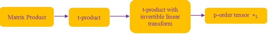
Figure 1: Relationship between Different Products

I use the idea of [16] and also introduce the matrix slices of $p$-order tensors. We can see the Figure 1 showing the relationship between different products. The product on the right is the generalization of that on the left. I denote the matrix slice of $\mathcal{A}$ as $\mathcal{A}^{{}^{\prime}}$, a third order tensor. We will discuss $p$-order tensors $\mathcal{A}\in\mathbb{C}^{n_{1}\times l\times\cdots\times n_{p}}$ and $\mathcal{B}\in\mathbb{C}^{l\times n_{2}\times\cdots\times n_{p}}$. First define $\triangle_{p}$ as a generalized case of $\triangle$,

Definition 12.

$$(\mathcal{A}\triangle_{p}\mathcal{B})^{{}^{\prime}(i)}=\mathcal{A^{{}^{\prime}}}^{(i)}\mathcal{B^{{}^{\prime}}}^{(i)},i=1,2,\cdots,n_{3}n_{4}\cdots n_{p}.$$

Now I can introduce the $p$-order tensor product with invertible linear transform,

Definition 13.

Given invertible transform $L$, i.e. $L(\mathcal{A})=A\times_{3}\mathbf{T}_{n_{3}}\times_{4}\mathbf{T}_{n_{4}}\cdots\times_{p}\mathbf{T}_{n_{p}}$,define the product as $L(\mathcal{A}*_{L}\mathcal{B})=L(\mathcal{A})\triangle_{p}L(\mathcal{B})$. In particular, if $L$ is a unitary transform, we denote the product as $*_{u}$. $\mathbf{T}_{n_{i}},i=3,4,\cdots,n_{p}$ is the corresponding matrix of transform $L$.

As [16] shows that

$$(\mathbf{F}_{n_{p}}\otimes\mathbf{F}_{n_{p-1}}\otimes\cdots\otimes\mathbf{F}_{n_{3}}\otimes\mathbf{I}_{n_{1}})\cdot\tilde{\mathbf{A}}\cdot(\mathbf{F}_{n_{p}}^{(-1)}\otimes\mathbf{F}_{n_{p-1}}^{(-1)}\otimes\cdots\otimes\mathbf{F}_{n_{3}}^{(-1)}\otimes\mathbf{I}_{n_{2}}),$$ (2)

we can diagonalize $\tilde{\mathbf{A}}$ in blocks. We may perform many times of $\mathtt{MatVec}$ to obtain $\tilde{\mathbf{A}}$ from $p$-order tensors. The diagonal block is like $(L(\mathcal{A}))^{{}^{\prime}(i)}$. Note that $L^{-1}(\mathcal{A})=A\times_{p}\mathbf{T}_{n_{p}}^{-1}\times_{n_{p-1}}\mathbf{T}_{n_{p-1}}^{-1}\cdots\times_{3}\mathbf{T}_{3}^{-1}$. I also give an algorithm to compute the product of $p$-order tensors,

Algorithm 1 Calculate $*_{L}$ product of $p$-order tensors

0:  $\mathcal{A}\in\mathbb{R}^{n_{1}\times l\times\cdots\times n_{p}}$,$\mathcal{B}\in\mathbb{R}^{l\times n_{2}\times\cdots\times n_{p}}$

0:  $\mathcal{C}\in\mathbb{R}^{n_{1}\times n_{2}\times\cdots\times n_{p}}$

1:  for $i=3,\cdots,p$ do

2:     $\mathcal{A}=\mathcal{A}\times_{i}\mathbf{T}_{n_{i}};\mathcal{B}=\mathcal{B}\times_{i}\mathbf{T}_{n_{i}};$

3:  end for

4:  for $i=1,2,\cdots,n_{3}n_{4}\cdots n_{p}$ do

5:     $\mathcal{C}^{{}^{\prime}(i)}=\mathcal{A}^{{}^{\prime}(i)}\mathcal{B}^{{}^{\prime}(i)};$

6:  end for

7:  for $i=p,p-1,\cdots,3$ do

8:     $\mathcal{C}=\mathcal{C}\times_{i}\mathbf{T}_{n_{i}}^{-1}$

9:  end for

I give a generalized definition of identity tensors,invertible tensors,

Definition 14.

$\mathcal{I}\in\mathbb{C}^{n\times n\times n_{3}\cdots\times n_{p}}$ satisfying $L(\mathcal{I})^{{}^{\prime}(i)}=\mathbf{I}_{n},i=1,2,\cdots,n_{3}\cdots n_{p}$ is an identity tensor.

It is easy to verify that

$$L(\mathcal{I})\triangle_{p}L(\mathcal{A})=L(\mathcal{A})\triangle_{p}L(\mathcal{I})=L(\mathcal{A}).$$ (3)

Then we get $\mathcal{A}*_{L}\mathcal{I}=\mathcal{I}*_{L}\mathcal{A}=\mathcal{A}$.

Definition 15.

$\mathcal{A}\in\mathbb{C}^{n\times n\times n_{3}\times\cdots\times n_{p}}$ is invertible if there exists $\mathcal{A}^{-1}\in\mathbb{C}^{n\times n\times n_{3}\times\cdots\times n_{p}}$ subject to

$$\mathcal{A}*_{L}\mathcal{A}^{-1}=\mathcal{A}^{-1}*_{L}\mathcal{A}=\mathcal{I}.$$

Some theoretical results can be shown,

Lemma 1.

The $p$-order tensors is associative under $*_{L}$.

Proof.

$$\begin{split}(\mathcal{A}*_{L}\mathcal{B})*_{L}\mathcal{C}&=L^{-1}(L(\mathcal{A})\triangle_{p}L(\mathcal{B}))*_{L}\mathcal{C}\\ &=L^{-1}(L(\mathcal{A})\triangle_{p}L(\mathcal{B}))*_{L}\mathcal{C}\\ &=L^{-1}(L(L^{-1}(L(\mathcal{A})\triangle_{p}L(\mathcal{B})))\triangle_{p}L(\mathcal{C}))\\ &=L^{-1}((L(\mathcal{A})\triangle_{p}L(\mathcal{B}))\triangle_{p}L(\mathcal{C}))\\ &=L^{-1}(L(\mathcal{A})\triangle_{p}L(L^{-1}(L(\mathcal{B})\triangle_{p}L(\mathcal{C}))))\\ &=L^{-1}(L(\mathcal{A})\triangle_{p}(L(\mathcal{B})*_{L}\mathcal{C}))\\ &=\mathcal{A}*_{L}(\mathcal{B}*_{L}\mathcal{C}).\end{split}$$ (4)

∎

Tubes of $p$-order tensors are in $\mathbb{C}^{1\times 1\times n_{3}\times\cdots\times n_{p}}$,also denoted as $\mathring{\mathbf{a}}$.

Theorem 2.

The set of all tubes in $\mathbb{C}^{1\times 1\times n_{3}\times\cdots\times n_{p}}$ form a commutative ring under $*_{L}$.

Proof.

From the definition of $*_{L}$, we can show

$$\begin{split}\mathring{\mathbf{a}}*_{L}(\mathring{\mathbf{b}}+\mathring{\mathbf{c}})&=L^{-1}(L(\mathring{\mathbf{a}})\triangle_{p}L(\mathring{\mathbf{b}}+\mathring{\mathbf{c}}))\\ &=L^{-1}(L(\mathring{\mathbf{a}})\triangle_{p}L(\mathring{\mathbf{b}})+L(\mathring{\mathbf{a}})\triangle_{p}L(\mathring{\mathbf{c}}))\\ &=L^{-1}(L(\mathring{\mathbf{a}})\triangle_{p}L(\mathring{\mathbf{b}}))+L^{-1}(L(\mathring{\mathbf{a}})\triangle_{p}L(\mathring{\mathbf{c}}))\\ &=\mathring{\mathbf{a}}*_{L}\mathring{\mathbf{b}}+\mathring{\mathbf{a}}*_{L}\mathring{\mathbf{c}}.\end{split}$$ (5)

The proof of $(\mathring{\mathbf{a}}+\mathring{\mathbf{b}})*_{L}\mathring{\mathbf{c}}=\mathring{\mathbf{a}}*_{L}\mathring{\mathbf{c}}+\mathring{\mathbf{b}}*_{L}\mathring{\mathbf{c}}$ is similar to the above. We also know that

$$\mathring{\mathbf{a}}*_{L}\mathring{\mathbf{b}}=L^{-1}(L(\mathring{\mathbf{a}})\triangle_{p}L(\mathring{\mathbf{b}}))=L^{-1}(L(\mathring{\mathbf{b}})\triangle_{p}L(\mathring{\mathbf{a}}))=\mathring{\mathbf{a}}*_{L}\mathring{\mathbf{b}}.$$ (6)

∎

Definition 16 (Transpose).

$\mathcal{A}^{H}\in\mathbb{C}^{l\times n_{1}\times n_{3}\times\cdots\times n_{p}}$ is the transpose of $\mathcal{A}$ if $L(\mathcal{A}^{H})^{{}^{\prime}(i)}=(L(\mathcal{A})^{{}^{\prime}(i)})^{H}$.

The following propositions shows that the transpose of tensors keeps some properties of transposing matrices.

Proposition 1.

$(\mathcal{A}*_{L}\mathcal{B})^{H}=\mathcal{B}^{H}*_{L}\mathcal{A}^{H}$

Proof.

$$\begin{split}L(\mathcal{B}^{H}*_{L}\mathcal{A}^{H})^{{}^{\prime}(i)}&=(L(\mathcal{B}^{H})\triangle_{p}L(\mathcal{A}^{H}))^{(i)}\\ &=L(\mathcal{B}^{H})^{{}^{\prime}(i)}L(\mathcal{A}^{H})^{{}^{\prime}(i)}\\ &=(L(\mathcal{B})^{{}^{\prime}(i)})^{H}(L(\mathcal{A})^{{}^{\prime}(i)})^{H}\\ &=(L(\mathcal{A})^{{}^{\prime}(i)}L(\mathcal{B})^{{}^{\prime}(i)})^{H}\\ &=((L(\mathcal{A})\triangle_{p}L(\mathcal{B}))^{(i)})^{H}\\ &=(L(\mathcal{A}*_{L}\mathcal{B})^{{}^{\prime}(i)})^{H}.\end{split}$$ (7)

So we get $L(\mathcal{B}^{H}*_{L}\mathcal{A}^{H})=L((\mathcal{A}*_{L}\mathcal{B})^{H})$. ∎

The definition of a unitary tensor is given here,

Definition 17.

$\mathcal{Q}\in\mathbb{C}^{m\times m\times n_{3}\times\cdots\times n_{p}}$ is a unitary tensor if $\mathcal{Q}^{H}*_{L}\mathcal{Q}=\mathcal{Q}*_{L}\mathcal{Q}^{H}=\mathcal{I}$.

The following theorem is important.

Theorem 3 ($p$-order tensor t-SVD under $*_{L}$).

There exists unitary tensors $\mathcal{U}\in\mathbb{C}^{n_{1}\times n_{1}\times n_{3}\times\cdots\times n_{p}}$, $\mathcal{V}\in\mathbb{C}^{l\times l\times n_{3}\times\cdots\times n_{p}}$ and $\mathcal{S}$ whose dimension is equal to that of $\mathcal{A}$ subject to $\mathcal{A}=\mathcal{U}*_{L}\mathcal{S}*_{L}\mathcal{V}^{H}$. Also, $\mathcal{S}_{i_{1}i_{2}\cdots i_{p}}\neq 0$ if and only if $i_{1}=i_{2}$.

Proof.

Let $\hat{\mathcal{A}}=L(\mathcal{A})$. Compute the matrix SVD of $\hat{\mathcal{A}}^{{}^{\prime}(i)}$, i.e.

$$\hat{\mathcal{A}}^{{}^{\prime}(i)}=\hat{\mathcal{U}}^{{}^{\prime}(i)}\hat{\mathcal{S}}^{{}^{\prime}(i)}(\hat{\mathcal{V}}^{{}^{\prime}(i)})^{H}.$$

Let $\mathcal{U}=L^{-1}(\hat{\mathcal{U}})$. $\mathcal{S}=L^{-1}(\hat{\mathcal{S}})$ and $\mathcal{V}=L^{-1}(\hat{\mathcal{V}})$. We need to prove that $\mathcal{U}$ is a unitary tensor. The proof of $\mathcal{V}$ is similar.

$$\begin{split}L(\mathcal{U}*_{L}\mathcal{U}^{H})^{{}^{\prime}(i)}&=(L(\mathcal{U})\triangle_{p}L(\mathcal{U}^{H}))^{(i)}=L(\mathcal{U})^{{}^{\prime}(i)}L(\mathcal{U^{H}})^{{}^{\prime}(i)}\\ &=\hat{\mathcal{U}}^{{}^{\prime}(i)}(\hat{\mathcal{U}}^{{}^{\prime}(i)})^{H}=\mathbf{I}_{n_{1}}=L(\mathcal{I})^{{}^{\prime}(i)},\end{split}$$ (8)

So $\mathcal{U}*_{L}\mathcal{U}^{H}=\mathcal{I}$ and the conclusion follows. ∎

If $\mathcal{C}=\mathcal{A}^{H}*_{L}\mathcal{A}$, $L(\mathcal{C})^{{}^{\prime}(i)}$ is positive semidefinite because

$$L(\mathcal{C})^{{}^{\prime}(i)}=L(\mathcal{A}^{H})^{{}^{\prime}(i)}L(\mathcal{A})^{{}^{\prime}(i)}=(L(\mathcal{A})^{{}^{\prime}(i)})^{H}L(\mathcal{A})^{{}^{\prime}(i)}.$$ (9)

The tensor determinant can be defined but now it is not a number.

Definition 18 (Tensor Determinant).

The determinant, which is in $\mathbb{C}^{1\times 1\times n_{3}\times\cdots\times n_{p}}$, of $\mathcal{A}\in\mathbb{C}^{2\times 2\times n_{3}\times\cdots\times n_{p}}$ can be defined as $\mathtt{det}(\mathcal{A})=|\mathcal{A}|=\mathring{\mathbf{a}}_{11}*_{L}\mathring{\mathbf{a}}_{22}-\mathring{\mathbf{a}}_{12}*_{L}\mathring{\mathbf{a}}_{21}$ where $\mathring{\mathbf{a}}_{ij}=\mathcal{A}(i,j,:,\cdots,:)$. We can define the determinant of $\mathcal{A}\in\mathbb{C}^{3\times 3\times n_{3}\times\cdots\times n_{p}}$ by unfolding the rows,

$$|\mathcal{A}|=\mathring{\mathbf{a}}_{11}*_{L}\begin{vmatrix}\mathring{\mathbf{a}}_{22}&\mathring{\mathbf{a}}_{23}\\ \mathring{\mathbf{a}}_{32}&\mathring{\mathbf{a}}_{33}\end{vmatrix}-\mathring{\mathbf{a}}_{12}*_{L}\begin{vmatrix}\mathring{\mathbf{a}}_{21}&\mathring{\mathbf{a}}_{23}\\ \mathring{\mathbf{a}}_{31}&\mathring{\mathbf{a}}_{33}\end{vmatrix}+\mathring{\mathbf{a}}_{13}*_{L}\begin{vmatrix}\mathring{\mathbf{a}}_{21}&\mathring{\mathbf{a}}_{22}\\ \mathring{\mathbf{a}}_{31}&\mathring{\mathbf{a}}_{32}\end{vmatrix}.$$

By recursion, we can define the determinant of $\mathcal{A}\in\mathbb{C}^{n\times n\times n_{3}\times\cdots\times n_{p}}$ now,

$$\mathtt{det}(\mathcal{A})=\sum_{j=1}^{n}(-1)^{j-1}\mathring{\mathbf{a}}_{1j}*_{L}\mathtt{det}(\mathcal{M}_{1j}),$$

where $\mathcal{M}_{1j}$ is a cofactor tensor.

We give an easy way to compute the determinant,

Theorem 4.

To compute the tensor determinant, we can first compute the determinant of $L(\mathcal{A})^{{}^{\prime}(i)}$, denoted by $\mathring{\mathbf{d}}^{{}^{\prime}(i)}$. Then compute $L^{-1}(\mathring{\mathbf{d}})$.

Proof.

If $\mathcal{A}\in\mathbb{C}^{2\times 2\times n_{3}\times\cdots\times n_{p}}$,

$$\begin{split}\mathtt{det}(\mathcal{A})&=L^{-1}(L(\mathring{\mathbf{a}}_{11})\triangle_{p}L(\mathring{\mathbf{a}}_{22}))-L^{-1}(L(\mathring{\mathbf{a}}_{21})\triangle_{p}L(\mathring{\mathbf{a}}_{12}))\\ &=L^{-1}(L(\mathring{\mathbf{a}}_{11})\triangle_{p}L(\mathring{\mathbf{a}}_{22})-L(\mathring{\mathbf{a}}_{21})\triangle_{p}L(\mathring{\mathbf{a}}_{12}))\end{split}$$ (10)

Note that $L(\mathring{\mathbf{a}}_{11})^{{}^{\prime}(i)}L(\mathring{\mathbf{a}}_{22})^{{}^{\prime}(i)}-L(\mathring{\mathbf{a}}_{12})^{{}^{\prime}(i)}L(\mathring{\mathbf{a}}_{21})^{{}^{\prime}(i)}$ is the matrix determinant of $L(\mathcal{A})^{{}^{\prime}(i)}$. If $n\geq 3$, the case of $\mathbb{C}^{(n-1)\times(n-1)\times n_{3}\times\cdots\times n_{p}}$ is right. For $\mathcal{A}\in\mathbb{C}^{n\times n\times n_{3}\times\cdots\times n_{p}}$, let the cofactor tensor of $\mathcal{A}$ be $\mathcal{M}_{1j}$ and the matrix determinant of $L(\mathcal{M}_{1j})^{{}^{\prime}(i)}$ be $\mathring{\mathbf{d}}_{1j}^{{}^{\prime}(i)}$. Then

$$\begin{split}L(\mathtt{det}(\mathcal{A}))&=\sum_{j=1}^{n}(-1)^{j-1}L(\mathring{\mathbf{a}}_{1j})\triangle_{p}L(\mathtt{det}(\mathcal{M}_{1j})\\ &=\sum_{j=1}^{n}(-1)^{j-1}L(\mathring{\mathbf{a}}_{1j})\triangle_{p}\mathring{\mathbf{d}}_{1j}\end{split}$$ (11)

So we get

$$L(\mathtt{det}(\mathcal{A}))^{{}^{\prime}(i)}=\sum_{j=1}^{n}(-1)^{j-1}L(\mathring{\mathbf{a}}_{1j})^{{}^{\prime}(i)}\mathring{\mathbf{d}}_{1j}^{{}^{\prime}(i)}=\mathring{\mathbf{d}}^{{}^{\prime}(i)}$$ (12)

Then $\mathtt{det}(\mathcal{A})=L^{-1}(\mathring{\mathbf{d}})$ and the conclusion follows. ∎

Theorem 5.

$\mathtt{det}(\mathcal{A}*_{L}\mathcal{B})=\mathtt{det}(\mathcal{A})*_{L}\mathtt{det}(\mathcal{B})$, where $\mathcal{A}$, $\mathcal{B}\in\mathbb{C}^{n\times n\times n_{3}\times\cdots\times n_{p}}$.

Proof.

$$\begin{split}\mathtt{det}(\mathcal{A})*_{L}\mathtt{det}(\mathcal{B})&=L^{-1}(L(L^{-1}(\mathring{\mathbf{d}}_{1}))\triangle_{p}L(L^{-1}(\mathring{\mathbf{d}}_{2})))\\ &=L^{-1}(\mathring{\mathbf{d}}_{1}\triangle_{p}\mathring{\mathbf{d}}_{2})\end{split}$$ (13)

where $\mathring{\mathbf{d}}_{1}$ and $\mathring{\mathbf{d}}_{2}$ are the tensors computed by the matrix determinant of $\mathcal{A}^{{}^{\prime}(i)},\mathcal{B}^{{}^{\prime}(i)}$ respectively. Let $\mathcal{C}=\mathcal{A}*_{L}\mathcal{B}$. Then $\mathcal{C}^{{}^{\prime}(i)}=\mathcal{A}^{{}^{\prime}(i)}\mathcal{B}^{{}^{\prime}(i)}$. And we need to compute the determinant, $\mathtt{det}(\mathcal{C}^{{}^{\prime}(i)})=\mathtt{det}(\mathcal{A}^{{}^{\prime}(i)})\mathtt{det}(\mathcal{B}^{{}^{\prime}(i)})$. We denote $\mathring{\mathbf{d}}_{3}$as the tensor computed by matrix determinant of $\mathcal{C}^{{}^{\prime}(i)}$ so $\mathring{\mathbf{d}}_{3}=\mathring{\mathbf{d}}_{1}\triangle_{p}\mathring{\mathbf{d}}_{2}$. Then

$$\mathtt{det}(\mathcal{C})=L^{-1}(\mathring{\mathbf{d}}_{3})=\mathtt{det}(\mathcal{A})*_{L}\mathtt{det}(\mathcal{B}).$$ (14)

∎

Theorem 6.

$$\mathtt{det}(\mathcal{I})=L^{-1}(\mathbf{1}_{1\times 1\times n_{3}\times\cdots\times n_{p}}),$$

where each element of $\mathbf{1}_{1\times 1\times n_{3}\times\cdots\times n_{p}}$ is 1.

Proof.

From the definition of identity tensors, we know that $\mathtt{det}(L(\mathcal{I})^{{}^{\prime}(i)})=1$. Then $\mathring{\mathbf{d}}=\mathbf{1}_{1\times 1\times n_{3}\times\cdots\times n_{p}}$. From the Theorem 4,

$$\mathtt{det}(\mathcal{I})=L^{-1}(\mathring{\mathbf{d}})=L^{-1}(\mathbf{1}_{1\times 1\times n_{3}\times\cdots\times n_{p}}).$$ (15)

∎

3 Tensor Nuclear Norm and Multi-rank

In this section I will give the definition of tensor nuclear norm and tensor multi-rank. Then I prove a theorem to show their relationship.

The multi-rank can be generalized.

Definition 19.

The multi-rank of $\mathcal{A}$ is defined as

$$\mathbf{rank}_{m}(\mathcal{A})=(\mathrm{rank}(\mathcal{A}^{{}^{\prime}(1)}),\mathrm{rank}(\mathcal{A}^{{}^{\prime}(2)}),\cdots,\mathrm{rank}(\mathcal{A}^{{}^{\prime}(n_{3}\cdots n_{p})})).$$

Given a linear invertible transform, we can define a tensor nuclear norm and spectral norm,

Definition 20.

The tensor nuclear norm and the tensor spectral norm under $*_{L}$ are respectively

$$\|\mathcal{A}\|_{*,L}=\sum_{i=1}^{n_{3}\cdots n_{p}}\|L(\mathcal{A})^{{}^{\prime}(i)}\|_{*},\|\mathcal{A}\|=\|\mathtt{bdiag}({L(\mathcal{A})}^{{}^{\prime}})\|.$$

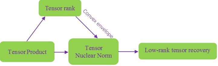
Figure 2: Overview of Low-Rank Tensor Recovery

I briefly show the idea of low-rank tensor recovery in Figure 2. We may use low-rank matrix recovery applying in unfolding tensors. But it will lead to curse of dimensionality and damage the inherent structure. We refer the readers to the recent work [7, 18] for details of low-rank tensor recovery models. Here I give a theorem to pave the way for the research about $p$-order tensor low-rank recovery. [18] gives a generalization under $*_{u}$.We need to use the fact that the tensor nuclear norm is the convex envelope of $\|\mathbf{rank}_{m}(\mathcal{A})\|_{1}$ to show the reasonableness of tensor nuclear norm including in the model. Consider the biconjugate and prove a theorem which generalizes the work of [18].

Theorem 7.

If $L$ is a unitary transform, $\|\mathcal{X}\|_{*,L}$ is the convex envelope of the $\ell_{1}$ norm of multi-rank on the set $\{\mathcal{X}|\|\mathcal{X}\|\leq 1\}$.

Proof.

Let $\Upsilon(\mathcal{X})=\|\mathbf{rank}_{m}(\mathcal{X})\|_{1}$ and $n_{(2)}=\min(n_{1},n_{2})$. If $\|\mathcal{X}\|\leq 1$, the conjugate of $\Upsilon(\mathcal{X})$ on the set where spectral norm is 1 can be defined as,

$$\Upsilon^{\#}(\mathcal{Y})=\sup_{\|\mathcal{X}\|\leq 1}(\mathrm{Re}(\langle\mathcal{Y},\mathcal{X}\rangle)-\|\mathbf{rank}_{m}(\mathcal{X})\|_{1}),$$ (16)

Using von Neumann’s trace inequality, we obtain

$$\begin{split}\mathrm{Re}(\langle\mathcal{Y},\mathcal{X}\rangle)&=\mathrm{Re}(\langle L(\mathcal{Y}),L(\mathcal{X}\rangle))=\sum_{i=1}^{n_{3}\cdots n_{p}}\mathrm{Re}(\mathrm{tr}((L(\mathcal{Y})^{{}^{\prime}(i)})^{H}L(\mathcal{X}^{{}^{\prime}(i)})))\\ &\leq\sum_{i=1}^{n_{3}\cdots n_{p}}|\mathrm{tr}((L(\mathcal{Y})^{{}^{\prime}(i)})^{H}L(\mathcal{X}^{{}^{\prime}(i)}))|\\ &\leq\sum_{i=1}^{n_{3}\cdots n_{p}}\sum_{j=1}^{n_{(2)}}\sigma_{j}(L(\mathcal{Y})^{{}^{\prime}(i)})\sigma_{j}(L(\mathcal{X})^{{}^{\prime}(i)})\end{split}$$ (17)

where $\sigma_{j}(\cdot)$ denotes the $j$-th biggest singular value of the matrix. We perform the $p$-order t-SVD on $\mathcal{Y}$ and then $\mathcal{Y}=\mathcal{U}_{y}*_{u}\mathcal{S}_{y}*_{u}\mathcal{V}_{y}^{H}$. Let $\mathcal{U}_{x}=\mathcal{U}_{y},\mathcal{V}_{x}=\mathcal{V}_{y}$ and choose $\mathcal{S}_{x}$ to make $\|\mathcal{X}\|\leq 1$. Then by the Theorem 3,

$$\begin{split}\mathrm{Re}(\langle\mathcal{Y},\mathcal{X}\rangle)&=\sum_{i=1}^{n_{3}\cdots n_{p}}\mathrm{Re}(\mathrm{tr}((L(\mathcal{Y})^{{}^{\prime}(i)})^{H}L(\mathcal{X}^{{}^{\prime}(i)})))\\ &=\sum_{i=1}^{n_{3}\cdots n_{p}}\mathrm{Re}(\mathrm{tr}(L(\mathcal{V}_{y})^{{}^{\prime}(i)}L(\mathcal{S}_{y})^{{}^{\prime}(i)}(L(\mathcal{U}_{y})^{{}^{\prime}(i)})^{H}L(\mathcal{U}_{x}^{{}^{\prime}(i)})L(\mathcal{S}_{x}^{{}^{\prime}(i)})(L(\mathcal{V}_{x}^{{}^{\prime}(i)}))^{H}))\\ &=\sum_{i=1}^{n_{3}\cdots n_{p}}\mathrm{Re}(\mathrm{tr}(L(\mathcal{V}_{y})^{{}^{\prime}(i)}L(\mathcal{S}_{y})^{{}^{\prime}(i)}L(\mathcal{S}_{x}^{{}^{\prime}(i)})(L(\mathcal{V}_{x}^{{}^{\prime}(i)}))^{H}))\\ &=\sum_{i=1}^{n_{3}\cdots n_{p}}\mathrm{Re}(\mathrm{tr}(L(\mathcal{S}_{y})^{{}^{\prime}(i)}L(\mathcal{S}_{x}^{{}^{\prime}(i)})))=\sum_{i=1}^{n_{3}\cdots n_{p}}\mathrm{tr}(L(\mathcal{S}_{y})^{{}^{\prime}(i)}L(\mathcal{S}_{x})^{{}^{\prime}(i)})\\ &=\sum_{i=1}^{n_{3}\cdots n_{p}}\sum_{j=1}^{n_{(2)}}\sigma_{j}(L(\mathcal{Y})^{{}^{\prime}(i)})\sigma_{j}(L(\mathcal{X})^{{}^{\prime}(i)})\end{split}$$ (18)

It shows we can obtain the equality. So

$$\Upsilon^{\#}(\mathcal{Y})=\sup_{\|\mathcal{X}\|\leq 1}(\sum_{i=1}^{n_{3}\cdots n_{p}}\sum_{j=1}^{n_{(2)}}\sigma_{j}(L(\mathcal{Y})^{{}^{\prime}(i)})\sigma_{j}(L(\mathcal{X})^{{}^{\prime}(i)})-\|\mathbf{rank}_{m}(\mathcal{X})\|_{1}),$$ (19)

Because $\|\mathbf{rank}_{m}(\mathcal{X})\|_{1}$ is an integer, the range of it is $[0,n_{(2)}n_{3}\cdots n_{p}]$.

If $\|\mathbf{rank}_{m}(\mathcal{X})\|_{1}=0$, then all singular values should be 0, i.e., $\Upsilon^{\#}(\mathcal{Y})=0$.

Let $n_{(2)}n_{3}\cdots n_{p}=N$. For all $1\leq r\leq N$ and an integer $r$, $\|\mathbf{rank}_{m}(\mathcal{X})\|_{1}=r$ and $\sigma_{(i)}(\mathcal{A})$ denotes the $i$-th biggest singular values of all matrix slices of $\mathcal{A}$. So

$$\Upsilon^{\#}(\mathcal{Y})=\max\{0,\sigma_{(1)}(L(\mathcal{Y}))-1,\cdots,\sum_{i=1}^{r}\sigma_{(i)}(L(\mathcal{Y}))-r\}$$ (20)

Then when $\|\mathcal{Y}\|\leq 1$,$\Upsilon^{\#}(\mathcal{Y})=0$. If there exists a positive integer $m$, not bigger than $r$, subject to,

$$\sigma_{(m)}(L(\mathcal{Y}))>1,\sigma_{(m)}(L(\mathcal{Y}))\leq 1,$$ (21)

then $\Upsilon^{\#}(\mathcal{Y})=\sum_{i=1}^{m}\sigma_{(i)}(L(\mathcal{Y}))-m$. Consider the conjugate of $\Upsilon^{\#}(\mathcal{Y})$ further,

$$\Upsilon^{\#\#}(\mathcal{Z})=\sup_{\mathcal{Y}}(\mathrm{Re}(\langle\mathcal{Z},\mathcal{Y}\rangle)-\Upsilon^{\#}(\mathcal{Y})),$$ (22)

Perform the $p$-order t-SVD on $\mathcal{Z}$ yields that $\mathcal{Z}=\mathcal{U}_{z}*_{u}\mathcal{S}_{z}*_{u}\mathcal{V}_{z}^{H}$. It is similar to get

$$\Upsilon^{\#\#}(\mathcal{Z})=\sup_{\mathcal{Y}}(\sum_{i=1}^{n_{3}\cdots n_{p}}\sum_{j=1}^{n_{(2)}}\sigma_{j}(L(\mathcal{Y})^{{}^{\prime}(i)})\sigma_{j}(L(\mathcal{Z})^{{}^{\prime}(i)})-\Upsilon^{\#}(\mathcal{Y}))$$ (23)

Then if $\|\mathcal{Z}\|>1$, let the biggest singular value of all matrix slices of $L(\mathcal{Z})$ be on the $k$-th matrix slice. In other words,

$$\sigma_{(1)}(L(\mathcal{Z}))=\sigma_{1}(L(\mathcal{Z})^{{}^{\prime}(k)}),$$ (24)

Choose $\|\mathcal{Y}\|>1$ to make $\sigma_{(1)}(L(\mathcal{Y}))=\sigma_{1}(L(\mathcal{Y})^{{}^{\prime}(k)})$

$$\begin{split}\Upsilon^{\#\#}(\mathcal{Z})&=\sup_{\mathcal{Y}}(\sum_{i=1}^{n_{3}\cdots n_{p}}\sum_{j=1}^{n_{(2)}}\sigma_{j}(L(\mathcal{Y})^{{}^{\prime}(i)})\sigma_{j}(L(\mathcal{Z})^{{}^{\prime}(i)})-(\sum_{i=1}^{m}\sigma_{(i)}(L(\mathcal{Y}))-m))\\ &=\sup_{\mathcal{Y}}\sigma_{(1)}(L(\mathcal{Y}))(\sigma_{(1)}(L(\mathcal{Z}))-1)+\sum_{i\neq k}\sum_{j=1}^{n_{(2)}}\sigma_{j}(L(\mathcal{Y})^{{}^{\prime}(i)})\sigma_{j}(L(\mathcal{Z})^{{}^{\prime}(i)})\\ &+\sum_{j=2}^{n_{(2)}}\sigma_{j}(L(\mathcal{Y})^{{}^{\prime}(k)})\sigma_{j}(L(\mathcal{Z})^{{}^{\prime}(k)})-(\sum_{i=2}^{m}\sigma_{(i)}(L(\mathcal{Y}))-m)\end{split}$$ (25)

$\sigma_{(1)}(L(\mathcal{Y}))$ can be sufficiently large, so the supremum is infinity. If $\|\mathcal{Z}\|\leq 1$ and $\|\mathcal{Y}\|\leq 1$, we get $\Upsilon^{\#}(\mathcal{Y})=0$. The supremum is obtained if $\sigma_{(i)}(L(\mathcal{Y}))=1,i=1,\cdots,N$ so

$$\Upsilon^{\#\#}(\mathcal{Z})=\sum_{i=1}^{N}\sigma_{i}(L(\mathcal{Z}))=\|Z\|_{*,u}$$ (26)

If $\|\mathcal{Y}\|>1$, let the singular value $\sigma_{(i)}(L(\mathcal{Y}))$ of matrix slice of $L(\mathcal{Y})$ correspond to $\sigma_{k(i)}(L(\mathcal{Z}))$ with regard to $\sum_{i=1}^{n_{3}\cdots n_{p}}\sum_{j=1}^{n_{(2)}}\sigma_{j}(L(\mathcal{Y})^{{}^{\prime}(i)})\sigma_{j}(L(\mathcal{Z})^{{}^{\prime}(i)})$, and then

$$\sum_{i=1}^{m}(\sigma_{k(i)}(L(\mathcal{Z}))-1)(\sigma_{(i)}(L(\mathcal{Y}))-1)\leq 0,\mbox{and}\sum_{i=m+1}^{N}\sigma_{k(i)}(L(\mathcal{Z}))(\sigma_{(i)}(L(\mathcal{Y}))-1)\leq 0,$$

so

$$\begin{split}\sum_{i=1}^{n_{3}\cdots n_{p}}&\sum_{j=1}^{n_{(2)}}\sigma_{j}(L(\mathcal{Y})^{{}^{\prime}(i)})\sigma_{j}(L(\mathcal{Z})^{{}^{\prime}(i)})-\sum_{i=1}^{m}(\sigma_{(i)}(L(\mathcal{Y}))-1)\\ &=\sum_{i=1}^{m}\sigma_{k(i)}(L(\mathcal{Z}))\sigma_{(i)}(L(\mathcal{Y}))+\sum_{i=m+1}^{N}\sigma_{k(i)}(L(\mathcal{Z}))\sigma_{(i)}(L(\mathcal{Y}))\\ &-\sum_{i=1}^{m}(\sigma_{i}(L(\mathcal{Y}))-1)-\sum_{i=1}^{N}\sigma_{(i)}(L(\mathcal{Z}))+\sum_{i=1}^{N}\sigma_{(i)}(L(\mathcal{Z}))\\ &=\sum_{i=1}^{N}\sigma_{(i)}(L(\mathcal{Z}))+\sum_{i=1}^{m}(\sigma_{k(i)}(L(\mathcal{Z}))-1)(\sigma_{(i)}(L(\mathcal{Y}))-1)\\ &+\sum_{i=m+1}^{N}\sigma_{k(i)}(L(\mathcal{Z}))(\sigma_{(i)}(L(\mathcal{Y}))-1)\leq\sum_{i=1}^{N}\sigma_{(i)}(L(\mathcal{Z}))\end{split}$$ (27)

On the set $\{\|\mathcal{Z}\|\leq 1\}$,$\Upsilon^{\#\#}(\mathcal{Z})=\sum_{i=1}^{N}\sigma_{(i)}(L(\mathcal{Z}))=\|\mathcal{Z}\|_{*,u}$. We get the conclusion exactly. ∎

4 Conclusion

In this paper, I propose a generalized kind of $p$-order tensor product using invertible linear transform. Given one transform, we may compute the tensor product efficiently. Also, after defining the tensor nuclear norm under this product and ranks, I prove a theorem to show the relationship between the multi-rank and tensor nuclear norm, which will facilitate the research of $p$-order tensor low-rank recovery. I also leave this direction to the future work. The generalized tensor determinant is defined as a tube. Its meaning needs to be thoroughly investigated in the future. Moreover, it is a little tricky to choose a good transform for a given data set. Given the insight from the theorem in [8], this topic should be studied deeper. In an operator perspective like [10], $p$-order tensor products may be analyzed further.

References

• [1] M. Belkin and P. Niyogi, Laplacian eigenmaps for dimensionality reduction and data representation, Neural computation, 15 (2003), pp. 1373–1396.
• [2] Y. Chang, L. Yan, H. Fang, S. Zhong, and Z. Zhang, Weighted low-rank tensor recovery for hyperspectral image restoration, arXiv preprint arXiv:1709.00192, (2017).
• [3] C. Eckart and G. Young, The approximation of one matrix by another of lower rank, Psychometrika, 1 (1936), pp. 211–218.
• [4] G. Ely, S. Aeron, N. Hao, and M. E. Kilmer, 5d seismic data completion and denoising using a novel class of tensor decompositions, Geophysics, 80 (2015), pp. V83–V95.
• [5] J. Håstad, Tensor rank is np-complete, in International Colloquium on Automata, Languages, and Programming, Springer, 1989, pp. 451–460.
• [6] F. L. Hitchcock, The expression of a tensor or a polyadic as a sum of products, Journal of Mathematics and Physics, 6 (1927), pp. 164–189.
• [7] Q. Jiang and M. Ng, Robust low-tubal-rank tensor completion via convex optimization, in Proceedings of the 28th International Joint Conference on Artificial Intelligence, Macao, China, 2019, pp. 10–16.
• [8] E. Kernfeld, M. Kilmer, and S. Aeron, Tensor–tensor products with invertible linear transforms, Linear Algebra and its Applications, 485 (2015), pp. 545–570.
• [9] H. A. Kiers, Towards a standardized notation and terminology in multiway analysis, Journal of Chemometrics: A Journal of the Chemometrics Society, 14 (2000), pp. 105–122.
• [10] M. E. Kilmer, K. Braman, N. Hao, and R. C. Hoover, Third-order tensors as operators on matrices: A theoretical and computational framework with applications in imaging, SIAM Journal on Matrix Analysis and Applications, 34 (2013), pp. 148–172.
• [11] M. E. Kilmer and C. D. Martin, Factorization strategies for third-order tensors, Linear Algebra and its Applications, 435 (2011), pp. 641–658.
• [12] T. G. Kolda and B. W. Bader, Tensor decompositions and applications, SIAM review, 51 (2009), pp. 455–500.
• [13] J. B. Kruskal, Rank, decomposition, and uniqueness for 3-way and n-way arrays, Multiway data analysis, (1989), pp. 7–18.
• [14] X. Li, Compressed sensing and matrix completion with constant proportion of corruptions, Constructive Approximation, 37 (2013), pp. 73–99.
• [15] C. Lu, J. Feng, W. Liu, Z. Lin, S. Yan, et al., Tensor robust principal component analysis with a new tensor nuclear norm, IEEE transactions on pattern analysis and machine intelligence, (2019).
• [16] C. D. Martin, R. Shafer, and B. LaRue, An order-p tensor factorization with applications in imaging, SIAM Journal on Scientific Computing, 35 (2013), pp. A474–A490.
• [17] O. Semerci, N. Hao, M. E. Kilmer, and E. L. Miller, Tensor-based formulation and nuclear norm regularization for multienergy computed tomography, IEEE Transactions on Image Processing, 23 (2014), pp. 1678–1693.
• [18] G. Song, M. K. Ng, and X. Zhang, Robust tensor completion using transformed tensor svd, arXiv preprint arXiv:1907.01113, (2019).
• [19] L. R. Tucker, Some mathematical notes on three-mode factor analysis, Psychometrika, 31 (1966), pp. 279–311.
• [20] Z. Zhang and S. Aeron, Exact tensor completion using t-svd, IEEE Transactions on Signal Processing, 65 (2016), pp. 1511–1526.
• [21] Z. Zhang, G. Ely, S. Aeron, N. Hao, and M. Kilmer, Novel methods for multilinear data completion and de-noising based on tensor-svd, in Proceedings of the IEEE conference on computer vision and pattern recognition, 2014, pp. 3842–3849.