Maximum bound principles for a class of semilinear parabolic equations and exponential time differencing schemes
Abstract
The ubiquity of semilinear parabolic equations has been illustrated in their numerous applications ranging from physics, biology, to materials and social sciences. In this paper, we consider a practically desirable property for a class of semilinear parabolic equations of the abstract form with being a linear dissipative operator and being a nonlinear operator in space, namely a time-invariant maximum bound principle, in the sense that the time-dependent solution preserves for all time a uniform pointwise bound in absolute value imposed by its initial and boundary conditions. We first study an analytical framework for some sufficient conditions on and that lead to such a maximum bound principle for the time-continuous dynamic system of infinite or finite dimensions. Then, we utilize a suitable exponential time differencing approach with a properly chosen generator of contraction semigroup to develop first- and second-order accurate temporal discretization schemes, that satisfy the maximum bound principle unconditionally in the time-discrete setting. Error estimates of the proposed schemes are derived along with their energy stability. Extensions to vector- and matrix-valued systems are also discussed. We demonstrate that the abstract framework and analysis techniques developed here offer an effective and unified approach to study the maximum bound principle of the abstract evolution equation that cover a wide variety of well-known models and their numerical discretization schemes. Some numerical experiments are also carried out to verify the theoretical results.
keywords:
Semilinear parabolic equation, maximum bound principle, numerical approximation, exponential time differencing, energy stability, error estimate.AMS:
35B50, 35K55, 65M12, 65R201 Introduction
Semilinear parabolic equations of the form
| (1) |
with being a time-dependent quantity of interests defined over a spatial domain , being a linear classic elliptic operator or its nonlocal variant, and representing a nonlinear operator, have been used to model numerous phenomena in nature. Many model equations like (1) and their solutions often satisfy some properties such as maximum principle, comparison principle, existence of invariant regions, and energy decay. These properties represent important physical features and are also essential for mathematical analysis and numerical simulations. For instance, classic reaction-diffusion equations can be seen as special cases of (1) where is given by a diffusion operator and is a reaction source: the diffusion process causes the concentration of some substance to spread in space and the reaction drives the dynamics based on the concentration values. One illustration is the dimensionless ignition model [62] for a supercritical high activation energy thermal explosion of a solid fuel in a bounded container, described by
| (2) |
Since the reaction term is always positive, the solution must reach its minimum either at the initial time or on the boundary of the domain, which is a popular form of the well-studied maximum principle for parabolic equations. Another popular example of (1) is the so-called Allen–Cahn equation [1], which takes on the form
| (3) |
with reflecting the width of the transition regions. The equation is also a special case of the Ginzburg–Landau theory that has been introduced earlier in the modeling of superconductivity [41] and other phase transition problems. It is well-known that the equation (3) and its more general form (as discussed later) hold a maximum bound principle (MBP) [19, 29]: if the initial data and/or the boundary values are pointwisely bounded by in absolute value, then the absolute value of the solution is also bounded by everywhere and for all time. This MBP is related to the conventional version of maximum principle described for (2), but also differs somewhat in scope, so we use a new name to distinguish them. For the scalar model like the equation (3), it is equivalent to the existence of special upper and lower solutions (the constant functions and respectively) of (3) under Dirichlet or homogeneous Neumann boundary condition [81]. Moreover, it can be also described as the equation (3) having a time-invariant region [2, 63, 91] since the region , of the value of the solution, remains unchanged during the time evolution. In this paper, we consider an abstract form of evolution equations given by (1) and focus on the problems having the MBP or the existence of the special form of the invariant region, namely, an upper bound on the pointwise absolute value of the solution (suitable defined for vector- and matrix-valued quantities). We note that the MBP is weaker than the conventional maximum principle in the sense that a problem satisfying a maximum principle must satisfy an MBP. Thus, the study of the conventional maximum principle, particularly with respect to the linear operator , plays relevant and important roles.
Whether the equation (1) has a maximum principle or not depends highly on the property of the linear operator . Concerning the linear operator , one can find from the standard textbooks on partial differential equations (see, e.g., [28]) that the equation (1) with the uniformly elliptic linear operator satisfies a maximum principle. During the past several decades, there have also been many studies devoted to the maximum principles for numerical approximations of linear elliptic operators. While it is too numerous to detail them all here, a partial list of earlier works includes the cases for finite difference method [5, 9, 83, 97], finite element method [3, 6, 7, 10, 61], collocation method [102, 103], and finite volume method [104]. In [9], a systematic analysis was presented on some sufficient conditions for the finite difference operator to satisfy the weak and strong maximum principles in the discrete sense. There were also works devoted to general analysis on algebraic properties of the approximating operators, which consist of the discrete maximum principles as special cases [32, 33, 73]. Extensions to parabolic cases have also been made. For example, [59] provided some sufficient conditions for the discrete maximum principles of the forward and backward Euler time-stepping methods, and additional researches can be found, e.g., in [30, 31, 60, 67, 69, 101]. In addition to the maximum principles for both linear elliptic differential operators and their finite dimensional discretizations, there are also some recent studies on the nonlocal analogues for linear nonlocal integral operators [22, 78, 94].
With the linear operator satisfying the conditions to yield the maximum principle, a suitable nonlinear term may lead to the existence of time-invariant regions of (1). The MBP, that is a special invariant region of the Allen–Cahn equation (3), was proved in [29]. An important and natural question for numerical analysis is whether such an MBP could be preserved by some time-stepping schemes for discretizing (3). This question has been studied in a variety of works recently. In [92], the discrete MBPs of a finite difference semi-discrete scheme and its fully discrete approximations with forward and backward Euler time-stepping methods were obtained for (3) in one-dimensional space. Later, the first-order stabilized implicit-explicit schemes with finite difference spatial discretization were proved to preserve the MBP [93], which was then generalized by [88] to the case with more general nonlinear terms. The discrete MBP was also obtained in [100] by proving the uniform boundedness of the average norm of the solution for any even integer , followed by passing the limit as goes to infinity. A first-order exponential time differencing (ETD) scheme (or say, exponential integrator scheme) in the space-continuous setting was analyzed in [24], where some properties of the heat kernel were used. In addition, the MBP-preserving numerical schemes have been also studied for the analogues of (3), such as the fractional Allen–Cahn equation using the Crank–Nicolson time-stepping [51], the nonlocal Allen–Cahn equation by using first- and second-order ETD schemes [20], and the complex-valued Ginzburg–Landau model of superconductivity [19] by considering the finite volume method [13] and finite element method with the mass-lumping technique [14] in space with backward Euler time-stepping.
In this paper, we present a unified framework on the MBPs for a class of semilinear parabolic equations (1) with general boundary conditions and their spatially discretized systems, as well as the time-discrete analogues of numerical approximations based on the exponential time differencing method. The ETD method [4, 11, 48] comes from the variation-of-constants formula with the nonlinear terms approximated by polynomial interpolations, followed by exact integration of the resulting integrals. We mainly address the following question: Under what conditions does the equation (1) have the MBP and do numerical approximations of (1) preserve the MBP? We provide an abstract framework on mathematical and numerical analysis for the MBP of (1), where the ETD method is used for the temporal discretization. Our main contribution includes several aspects. First, we systematically formulate an abstract mathematical framework to illustrate the essential characteristics of the linear and nonlinear operators in (1) so that the model equation satisfies the MBP and the corresponding first- and second-order ETD schemes preserve the discrete MBP unconditionally. Second, we are able to present results valid for a large class of semilinear parabolic problems subject to different boundary conditions and constraints which significantly generalize those obtained in [20] (which is a specialized study focused only on the nonlocal Allen–Cahn equation with periodic boundary condition). We demonstrate that the theory also works for problems subject to either Dirichlet boundary condition or homogeneous Neumann boundary condition in the classic (local continuum) and nonlocal sense. These generalizations offer our theory a much wider range of applicability. Third, in order to establish a broad and abstract framework presented here, new analysis techniques are developed. They differ from the ones used in earlier works. Indeed, the abstraction allows us to discover the essential ingredients of the MBPs, which were absent from earlier analysis. In addition, we also derive error estimates for the approximate solutions of MBP-preserving ETD schemes, as well as their energy stability when applied to gradient flow models.
The necessity to take nonhomogeneous Dirichlet boundary condition into account comes from various practical considerations. For instance, phase separations occurring in hydrocarbon systems could be described by a diffuse-interface model with the Peng–Robinson equation of state [84], where a nonhomogeneous Dirichlet boundary condition is usually needed to keep the microstructures with certain phases on the boundary. In addition, nonhomogeneous Dirichlet boundary conditions are also necessary for many scalable and multiscale algorithms based on domain and subspace decompositions.
One of the distinctive features of the ETD schemes is the exact evaluation of the contribution of the linear operator, which provides good stability and accuracy even though the linear part has strong stiffness. Besides, the ETD schemes usually perform as efficient as an explicit scheme since the operator exponentials could be often implemented by some fast algorithms in regular domains. Such advantages lead to successful applications of ETD schemes on a large class of phase-field models which usually yield highly stiff ODE systems under spatial discretizations. We refer the readers to the literature, e.g., [20, 55, 57, 58, 105, 107].
The rest of this paper is organized as follows. In Section 2, we recall the semilinear equation (1) in a Banach space consisting of real scalar-valued continuous functions, declare the basic assumptions on the linear and nonlinear operators, and show that the model equation has a unique solution and satisfies the MBP under these assumptions. We also present a variety of concrete examples of the linear and nonlinear operators in the space-continuous and space-discrete settings covered by the theoretical framework. In Section 3, first- and second-order ETD time-discrete schemes are constructed and proved to preserve the discrete MBPs along with their convergence analysis. In addition, energy stability is also analyzed when the framework is applied to gradient flow models. In Section 4, we discuss the extensions to vector-valued and matrix-valued problems in the space-continuous setting with the complex-valued one being a special case. In Section 5, practical implementations of the ETD schemes are discussed and some numerical experiments are also performed to verify the theoretical results. Finally, concluding remarks are given in Section 6.
2 Maximum bound principle of the model equation
2.1 Abstract framework
Let us assume is either a connected spatial region or a collection of isolated points in . More precisely, we consider the following two situations:
-
(D1)
is an open, connected and bounded set with a Lipschitz boundary denoted by , and is a closed connected set disjoint with but ; denote and ;
-
(D2)
for a given pair of sets and that are described in (D1), and with consisting of all the nodes in a mesh partitioning , we let , , , , and .
Note that in Case (D1), we have for classic differential operators and is usually a nonempty volume for nonlocal integral operators. When , we define and ; otherwise, we define and . For a problem with periodic boundary condition, we assume that its period cell is a rectangle in , i.e., , and we use a special notation . Case (D2) corresponds to a discrete version of (D1). This allows us to unify the discussions presented later with the same set of notations for both space-continuous and space-discrete cases. For any set , we denote by the space consisting of real scalar-valued continuous functions defined on and by the set of all bounded functions in . Here, the continuity of functions is defined as follows [86]:
| (4) |
If is bounded and closed, then obviously .
Let if ; otherwise and we write below for simplicity. Define the supremum norm on by
then becomes a Banach space. According to the definition (4), is well-defined under Cases (D1) and (D2). Let be a nonlinear operator and be a linear operator with the domain . Then we consider the following two cases:
-
(C1)
and , where ;
-
(C2)
, where is periodic with respect to the rectangle .
It is easy to see that defined in any of Cases (C1) and (C2) can be regarded as a linear subspace of in the sense of isometric isomorphism () through the zero or periodic extension to or correspondingly. We always omit the extension mapping between and for simplicity when there is no ambiguity. We also remark that equipped with the supremum norm is a Banach space in both Cases (C1) and (C2), so is in Case (C1).
For Case (D1), define which is a subspace of ; for Case (D2), define . Then we define the linear operator . Note that for any , it holds in , and is also well-defined in in the sense of isomorphism.
The model problem we consider in this paper is a class of semilinear parabolic equations taking the following form
| (5) |
where is the unknown function subject to the initial condition
| (6) |
with and either the periodic boundary condition for Case (C2) or the Dirichlet boundary condition
| (7) |
for Case (C1) with . The compatibility condition is also assumed to hold, that is, on for Case (C1) and is -periodic for Case (C2).
In order to establish the maximum bound principle (MBP) for the model problem (5), as well as its time discretizations proposed later, we make the following specific assumptions regarding the operators , and defined above.
Assumption 1 (Requirements on and ).
The linear operators and satisfy the following conditions:
(a) for any and , if
| (8) |
then ;
(b) the domain is dense in ;
(c) there exists such that the operator is surjective, where is the identity operator.
Note that it can be derived from Assumption 1-(a) that maps any constant function in to the zero element in .
Assumption 2 (Requirements on ).
The nonlinear operator acts as a composite function induced by a given one-variable continuously differentiable function , that is,
| (9) |
and there exists a constant such that
| (10) |
Remark 1.
A more general case is that the function satisfies for some instead of (10) in Assumption 2. In this case, one can carry out an affine transform to the unknown function . More precisely, take the affine transform defined by
and define for any , then it holds . By letting , we can obtain from (5) that
where the nonlinear mapping is determined by the composite function
and satisfies Assumption 2.
Lemma 1.
Under Assumption 1, the following properties on hold:
(i) is dissipative, i.e., for any and any ,
(ii) is the generator of a contraction semigroup on , i.e., , where denotes the operator norm defined by
Proof.
We first prove the result for Case (C1). For any , since and , it is clear that reaches its maximum at some point , namely, . Without loss of generality, let us assume ; otherwise, we consider instead. If , we know that by Assumption 1-(a). If , then by the definition of . For any , we then have
which completes the proof of (i). Then, according to (i), Assumptions 1-(b) and 1-(c), the property (ii) follows from the Lumer–Phillips Theorem [27, Theorem II.3.15].
Now we consider Case (C2) and such that . If , by the -periodicity, we can regard as a point in . Then, the above analysis could be similarly done to obtain (i) and (ii). ∎
Remark 2.
The proof of Lemma 1-(i) uses the Assumption 1-(a) (which is only related to ) and the definitions of and to deduce the fact that if (8) holds with . Lemma 1-(ii) is the consequence of Lemma 1-(i) and Assumption 1-(b) and (c). We note that Lemma 1-(ii) is the key result to be used in later discussions. It can be established under different assumptions by using other approaches, see discussions in Example 2.6.
Next, let us introduce a stabilizing constant and rewrite the equation (5) in the following equivalent form:
| (11) |
where . According to (9) in Assumption 2, we know
where
| (12) |
We impose a requirement on the selection of the stabilizing constant as
| (13) |
Note that (13) always can be reached since is continuously differentiable.
Proof.
Now we can show that the aforementioned model problem admits a unique solution and possesses the MBP. Our main theorem can be stated as follows.
Theorem 3.
Proof.
Let us consider Case (C1) first. Denote and for any . For a fixed and a given , let us define to be the solution of the following linear problem:
| (15) |
where the constant satisfies (13). It is easy to know that is uniquely defined on by noticing that setting , , and in (15) leads to , and thus for each . Suppose there exists such that . By (14b), we only need to consider the case . According to Assumption 1-(a), we have and at , which implies . Since , according to Lemma 2-(i), we obtain . Similarly, if there exists such that , one can show . Thus we obtain for any , which means .
Next we define a mapping by through (15). For , we see that and satisfy
Using Lemma 2-(ii), we can estimate the difference between and by
then,
When , we see that is a contraction. Since is closed in , we know that is complete with respect to the metric reduced by the norm . Then we can apply Banach’s fixed-point theorem to get the existence of a unique solution to the model equation (5) on . Using standard continuation argument, we then have the global existence of the unique solution for any .
For Case (C2), the system (15) still holds after removing the second equation in it. For the case , by the periodicity, we could regard as a point in . Then, the analysis above is still valid. Putting all the different cases together, we get a complete proof. ∎
Remark 3.
We note that Theorem 3 also could be proved using other classical methods, such as the method of upper and lower solutions [81] in the case of scalar second-order elliptic operator. We emphasize that, in the proof given here, the MBP of the model equation (5) has no explicit dependence on the constant , even though we have assumed that satisfies (13) in order to use the Lemma 2. Meanwhile, we will see later that the choice of the constant plays an important role in designing MBP-preserving ETD schemes.
In the following subsections, we present some examples of the nonlinear and linear operators which are applicable to the mathematical framework established above.
2.2 Examples of the nonlinear function
One usually chooses as with being a primitive function, when considering the phase-field models, or says, the gradient flows of some free energy functionals.
Example 2.1.
Consider the function
| (16) |
where and . According to Remark 1, satisfies that with any and . Especially, for an even integer , one can choose such that satisfies Assumption 2, then the requirement (13) becomes . The special case gives the well-known logistic function and the case with gives
| (17) |
the derivative of with (the quartic double-well potential).
Example 2.2.
Example 2.3.
The Peng–Robinson equation of state [82] is widely used in the oil industries and petroleum engineering. The Helmholtz free-energy density considered in such a model can be expressed as
where is the universal gas constant, the temperature, the energy parameter, and the covolume parameter. The values of these parameters could be found in [84]. Then
| (20) |
which has two zero points and satisfying . This example falls into the situation discussed in Remark 1.
2.3 Examples of the linear operator
2.3.1 Infinite dimensional examples
Here we present some examples of the linear operator in the form of classic differential or nonlocal integral operators corresponding to Case (D1). We will verify that and the induced operator satisfy Assumption 1.
Example 2.4 (Second-order elliptic differential operator).
Consider the linear operator
| (21) |
where and is symmetric and positive definite uniformly (i.e., there exists such that for all and ). In this case, , , , the boundary condition (7) is the classic Dirichlet one, , and . For any and such that (8) holds, we always have and is negative semi-definite. Since is symmetric, there exists an orthogonal matrix such that
with for all . Thus, we have
Since is symmetric and negative semi-definite, its diagonal entries are all non-positive. Thus, we obtain and then , which gives Assumption 1-(a). Assumption 1-(b) is guaranteed by the fact that and for Case (C1), and and for Case (C2) in the sense of isomorphism. Assumption 1-(c) can be obtained from the standard analysis of the existence and regularity of the solution to the partial differential equation in for any and .
Remark 4.
Example 2.5 (Nonlocal diffusion operator).
Consider the integral operator [17]
| (23) |
where is a symmetric nonnegative kernel function, i.e., . We consider the widely studied case of the nonlocal operator (23), in which the kernel is radial and parameterized by a horizon parameter much less than the size of , i.e., for some nonnegative function with and for some constant . In this case, , , , the boundary condition (7) becomes a volume constraint, and . Then, the operator (23) can be re-expressed as
| (24) | |||||
For suitable subject to the finite second-order moment condition:
the operator is consistent with the standard Laplacian as (see, e.g., [15, 17]). Assumption 1-(a) results from the nonnegativity of the kernel. Whether Assumptions 1-(b) and 1-(c) are satisfied depends on the choice of the kernel. Let us consider the situation of integrable kernels only (i.e., ), for which and for any . Here, denotes the convolution and . For Case (C1), we have and in the sense of isomorphism using zero extension to thus Assumption 1-(b) follows automatically. For any and , there exists a unique solution to the equation in , and it further can be shown [8, 23] by the property that the convolution of and functions is uniformly continuous, which verifies Assumption 1-(c). For Case (C2), we have and all the assumptions are still satisfied. Regarding non-integrable kernels with strong singularity at the origin like the fractional power, we refer to discussion in the next example.
Example 2.6 (Fractional Laplace operator).
For a fixed , the fractional Laplace operator is the pseudo-differential operator with symbol , that is,
where , the class of Schwarz functions, and denotes the Fourier transform. Denoting , an equivalent form of on a bounded spatial domain is given by [87]
| (25) |
with . In this case, , , and . As shown in [96], the operator could be regarded as the limit, when , of the nonlocal operator defined by (24) equipped with a special rescaled and truncated fractional kernel for . Let us consider Case (C1) only, for which in the sense of isomorphism using zero extension to . Define as the restriction of on . Due to the lack of full elliptic regularity, Lemma 1 is not readily applicable. However, we can still get Lemma 1-(ii) using the Beurling–Deny criteria [80]. Indeed, as proved in [36] if the boundary is and still valid if is Lipschitz, the equation in subject to with the initial data has a unique weak solution for all , i.e., and
for any with . To obtain Lemma 1-(ii), i.e., the solution induces a contraction semigroup on with respect to the supremum norm , it suffices to show that for any with on , one has in . The latter can be checked by taking in the above weak form to get that
which deduces
thus in . With Lemma 1-(ii) established, the first part of the proof of Theorem 3 can also be modified accordingly so that the same theorem remains valid.
To sum up, for the above examples, we can obtain the following result on the MBP according to Theorem 3.
Corollary 4.
2.3.2 Finite dimensional examples
We consider some concrete linear operators for the situation of , in particular, the case of is given by Case (D2). Let us denote by the linear operator, with the subscript used to distinguish it from the notation in the infinite dimensional cases. Without loss of generality, we assume that is the node set of a uniform Cartesian mesh on the hypercube . The choice of uniform mesh simplifies the notation but we note that the analysis can be extended to non-uniform and non-Cartesian grids as discussed later with respect to finite element (or finite volume) discretizations. With the uniform Cartesian mesh, for a given and the uniform mesh size , let , , and . Thus, is isomorphic to with the norm equivalent to the vector infinity-norm. Here, for Case (C1), we let if and otherwise, while for Case (C2). The mesh can be extended as needed to represent , and the solution on (mesh nodes in ) is explicitly given for Case (C1) or can be obtained from that on by the periodicity of the solution in for Case (C2).
We may view the grid function as a vector with denoting the values of at nodes (for Case (C1)) or (for Case (C2)) ordered lexicographically. Then, the nonlinear mapping plays a role as a vector-valued function satisfying
In addition, due to the discrete nature, we now have that and the linear operator is equivalent to , which is an -by- matrix. Thus, the semigroup generated by is actually the matrix exponential . In these settings, Assumption 1-(b) is trivial and Assumption 1-(c) could be verified more directly by the following result.
Proposition 5.
Example 2.7 (Central difference operator for the Laplacian).
To make the discussion more clearly, let us begin with the one-dimensional case. Now, . For Case (C1), we have . For any , the second-order central difference approximation of the Laplacian is defined by
| (27) |
for with and determined by the boundary condition. For Case (C2), for a grid function , we still define as (27) for but with and due to the periodicity. Assumption 1-(a) holds according to (27). Define
and satisfies (26) obviously. We have , so Assumption 1-(c) is satisfied.
For the two- and three-dimensional cases, we define as a summation of the central difference approximations in every coordinate direction given as (27). Thus, satisfies Assumption 1-(a). Also, we can present the matrix by using the Kronecker products as
| (28) | ||||
| (29) |
where is the identity matrix, and the vectors determined by the boundary conditions could be given in the similar way. It is easy to check that corresponding to (28) or (29) satisfies Assumption 1-(c).
Remark 6.
It is well-known that (28) provides the central difference approximation of the Laplacian in the two-dimensional case. However, if one considers more general elliptic operators, such as (21), including mixed partial derivatives and a convection term, the corresponding discretized operator cannot be written in the form of Kronecker products. Instead, the upwind formulas are adequate to discretize the derivatives in the convection term and those in the mixed partial derivatives. The detailed analysis of the resulted linear operator is quite similar to Example 2.7 and we omit it. A general formulation for the finite difference approximation of (21) could be found in [9], where a sufficient and necessary condition (more general than Proposition 5) is given for the discrete MBP of the approximating operator.
Example 2.8 (Quadrature-based difference operator for the nonlocal diffusion).
Recalling the nonlocal diffusion operator (24), we consider its quadrature-based finite difference discretization, which is well known to be asymptotically compatible [22, 95]. The dimension of clearly depends on the value of in this case. For a given , we define at for Case (C1) or for Case (C2) via
| (30) |
where the values of with could be supplementally defined using the boundary conditions so that the operator (30) is well-defined. Here, stands for the vector -norm, and
where is the piecewise -multilinear basis function satisfying when and . It is obvious that given by (30) satisfies Assumption 1-(a). By ordering the nodes lexicographically, we regard the function as a vector in and it is easy to check that the matrix , the restriction of on , is diagonally dominant in the sense of (26). Thus, Assumption 1-(c) is satisfied. Moreover, is a band matrix with the bandwidth depending on the value of .
Example 2.9 (Finite difference operator for the fractional Laplacian).
For the fractional Laplace operator (25), we consider its finite difference discretization in Case (C1), and for simplicity the homogeneous Dirichlet boundary condition is enforced so that the operators and are essentially the same in this case. For the one-dimensional case, a second-order finite difference discretization [25, 52] (a limiting case of a similar scheme given in [95] for nonlocal diffusion models) is defined by:
| (31) |
for any , where the entries of the matrix are given by
for , where with or . Obviously, the matrix is diagonally dominant in the sense of (26), and thus Assumptions 1-(a) and 1-(c) are satisfied. For the two- and three-dimensional cases, the operators and could be given in the similar way, we refer to [26, 52] for details, and it is easy to verify that Assumption 1 is still satisfied.
Example 2.10 (Finite element operator for the Laplacian).
Let us consider Case (C1) again. Let be a uniform partition of into isosceles right triangles non-overlapping with each other based on the set of nodes . Let be the space of continuous and piecewise linear functions with respect to and be its subspace with zero-trace:
We denote by and the numbers of the nodes in and on respectively, and order the nodes such that consisting of all interior nodes and all nodes on the boundary. Denote by the basis functions of satisfying for any . Define the operator for by
| (32) |
where
For each , it is known that
| (33) |
Noticing that on , we have that
| (34) |
Combination of (33) and (34) yields
| (35) |
for and , which implies Assumption 1-(a). The limitation of on is given by the matrix with , . Then, by (35), satisfies (26) and Assumption 1-(c) holds.
Remark 7.
For a general partition of , the FEM-based linear operator could be also defined by (32) and still satisfies (26), see, e.g., [78] for discussions. In fact, it is well-known in the literature that the discrete maximum principle holds for piecewise linear finite element approximations of the Laplacian on general two-dimensional Delaunay triangulations for which the circumscribing circle of any Delaunay triangle does not contain any other vertices in its interior, see [21]. The brief note [7] analyzes a stabilized Galerkin approximation of the Laplacian guaranteeing the discrete maximum principle on arbitrary meshes. In addition, one can also apply the finite volume method (FVM) [66] to obtain the discretized operator of the Laplacian. The FVM-based linear operator possesses similar properties as those we have considered in the above.
2.4 Discussion on homogeneous Neumann boundary conditions
In Section 2.1, the MBPs for the cases of Dirichlet and periodic boundary conditions are studied, let us now discuss the case of homogeneous Neumann boundary condition. For simplicity, we focus the analysis on the infinite dimensional operators. The key ingredient is to find a Neumann operator such that the following Gaussian formula holds:
The homogeneous Neumann boundary condition then could be given by
| (36) |
For the second-order elliptic operator in the divergence form (22), using the classic Gaussian formula and assuming is divergence-free, we obtain
where denotes the unit outward normal vector to . Thus, the Neumann operator could be defined as
and the corresponding constraint becomes the classic Robin boundary condition. Alternatively, if we apply the classic Gaussian formula only to the diffusion part , then could be also defined by
| (37) |
and the corresponding constraint becomes the classic Neumann boundary condition.
For the nonlocal diffusion operator defined in (23), by the symmetry of the kernel, we have
Then we have
where is defined by
This definition, different from those in [17, 18], can be found in [15] as a nonlocal extension of (37).
We next consider the model problem (5) subject to the homogeneous Neumann boundary condition (36). In order to show that the MBP is still satisfied for the above classic and nonlocal cases, we need to generate a contraction semigroup as before so that all the analysis conducted above could be similarly used. To this end, we still let if and otherwise, and Assumption 1-(a) is clearly true for the above two operators . Then we need to define and appropriately and verify whether all conditions related to them in Remark 2 hold.
For the classic elliptic differential operator case, without loss of generality, let us assume and in (21). For any , we can directly extend the domain of from to by continuity so that . Let us define , and , then Assumptions 1-(b) and 1-(c) obviously hold. For any , assume that (8) is true for some . By using the boundary condition ( and the reflective extension in classic analysis, we have that and the Hessian is negative semi-definite, and consequently it holds by using an orthogonal transformation of the coordinates. Thus, we can similarly show that Lemma 1-(i) is valid and consequently generates a contraction semigroup on (i.e., Lemma 1-(ii)).
Next we turn to the nonlocal diffusion operator case, where is defined by (24) with the integrable kernel as discussed in the Example 2.5. For any , there exists a unique satisfying and ; in particular, we have
| (38) |
By defining with , we can regard as a linear subspace of in the sense of isomorphism () using such Neumann extension. Assumption 1-(b) automatically comes from . For any and , it is also not hard to verify that the equation in has a unique solution in , similar to the discussion in the earlier example for the zero Dirichlet boundary condition, which implies Assumption 1-(c). For any , assume that (8) holds for some , then we know by (38) that the maximum of on must also be attained on . Thus, according to the proof of Lemma 1-(i), we see that its conclusion still remains valid, and consequently we obtain Lemma 1-(ii).
3 Exponential time differencing for temporal approximation
In this section, we construct temporal approximations of the model equation (5) by using the exponential time differencing (ETD) method. We will begin with the equivalent form (11) to develop the MBP-preserving ETD schemes of first- and second-order, followed by the convergence analysis. For all discussions and theorems established in this section, we only focus on Case (C1) while the results are all valid for Case (C2) by removing the equations containing the boundary term and using the periodicity of the solution in the proofs.
3.1 ETD schemes and discrete MBPs
Given a time step size , we divide the time interval by . To establish the ETD schemes for solving the model problem (5), we focus the equivalent equation (11) on the interval , or equivalently, satisfying the following system
| (39) |
For the first-order (in time) approximation of (39), we set to obtain the first-order ETD (ETD1) scheme: for and given , find with solving
| (40) |
where represents an approximation of and is given. Similar to (15), it is easy to show that is uniquely defined on , thus is well-defined. We note that unlike the continuous-in-time case, different choices of do lead to different discretization schemes. Indeed, serves as the generator of the semigroup to control the nonlinear term and then to stabilize the time discretizations. Thus, a suitable choice of becomes very important in our design of ETD schemes.
Theorem 7 (Maximum bound principle of the ETD1 scheme).
Proof.
Since , we just need to show that implies for any . We have , where satisfies (40) with the superscript replaced by . Suppose there exists such that
| (41) |
Similar to the first part of the proof of Theorem 3, we can obtain , and then, . The lower bound could be obtained similarly. Thus we obtain for any , and thus , which completes the proof. ∎
Next, we consider the higher-order approximations of the solution of (39). Let be an interpolation of with degree on the times . Then, we approximate by to obtain the higher-order ETD Runge–Kutta scheme: find with solving
where is an approximation of with . More precisely, we have
where are the standard Lagrange basis functions associated with the times , and is an approximated value of , generated by the lower-order ETD schemes and . In the spirit of the proof of Theorem 7, we know that the discrete MBP would be preserved as long as the following condition is satisfied:
| (42) |
with for all . However, the unique interpolation satisfying (42) corresponds to the case , that is, the linear interpolation
Approximating in (39) by , we obtain the second-order ETD Runge–Kutta (ETDRK2) scheme: find with solving
| (43) |
where is generated by the ETD1 scheme. It is worth noting that both ETD1 and ETDRK2 schemes are linear.
Theorem 8 (Maximum bound principle of the ETDRK2 scheme).
Proof.
As an application of Theorems 7 and 8, one can obtain the MBPs of the semi-discrete and fully discrete ETD schemes for the concrete examples presented in Sections 2.2 and 2.3.
Corollary 9.
For the space-continuous ETD1 and ETDRK2 schemes with given by any of (21), (24), and (25), as well as the fully discrete ETD1 and ETDRK2 schemes with the (discretized) linear operator defined by any of (27), (30), (31), or (32), it holds that
In summary, we have proved that the first- and second-order ETDRK schemes preserve the MBP of the underlying problem (5) unconditionally in the discrete sense. Meanwhile, we actually show that the classic ETDRK approximations, as defined in [11], with order greater than two fail to maintain the MBP unconditionally due to the lack of the property (42) for the interpolation polynomials with . Apart from the ETDRK schemes, multistep approximations could be also utilized in the ETD temporal discretization [49]. The ETD-multistep scheme of order is generated from the extrapolation polynomial of degree for the nonlinear term based on the approximated solutions at the previous time levels. Since the extrapolation polynomials with cannot be bounded by the maximums and minimums of the extrapolated data, the ETD-multistep schemes with even order greater than one also fail to preserve the discrete MBP unconditionally.
Up till now, we only presented the differential forms of the ETD1 and ETDRK2 schemes by (40) and (43) since they are convenient for the theoretical analysis. In practice, we need formulas that can be more directly implemented for computations, in particular, the fully discrete schemes (in both time and space) with and discussed in Section 2.3.2. Here we define a new operator as follows: for any and with , let
| (44) |
It is easy to check that the right-hand side of (44) depends only on , so is well-defined through (44).
For a given boundary data and a function such that , we obtain from (39) and the definition of that
| (45) |
where is an -by- matrix. Let
| (46) |
and define the -functions as follows:
Let . Then, we give the fully discrete ETD1 scheme by
| (47) |
or equivalently,
and the fully discrete ETDRK2 scheme by
or equivalently,
| (48) |
Note that the corresponding semigroup is given by the matrix exponential , which again depends crucially on the choice of the constant .
3.2 Convergence analysis of the ETD schemes
As an important application of the MBP, we now consider the convergence of the ETD1 and ETDRK2 schemes. From the practical point of view, we are mainly interested in the convergence of the fully discrete solution to the semi-discrete (in space) solution (with a fixed spatial mesh size) as the time step size goes to zero. Again, we have and as we discussed in Section 2.3.2. First, let us state the result for the ETD1 scheme (40).
Theorem 10.
Suppose that Assumptions 1 and 2, (13) and (14) are satisfied. For the fixed terminal time and spatial mesh size , assume that the exact solution to the space-discrete model equation (45) belongs to and is generated by the fully discrete ETD1 scheme (47) with . Then we have
| (49) |
for any , where the constant depends on the norm of , but independent of and .
Proof.
We know that the ETD1 solution is given by with the function solving
| (50) |
Let . The difference between (50) and (45) yields
| (51) |
where is the truncated error as
Due to the MBP of (5), we have and , and then, using Lemma 2-(ii), we derive
where the constant depends on the norm of , but independent of and . Similarly, since , we can obtain
| (52) |
Then, we derive from (51) that
| (53) |
where in the last step we have used the fact that for any . By induction, we have
By letting , we obtain (49) since and . ∎
Remark 8.
We note that in the estimate (49), there is an exponential coefficient which could be very large (e.g., in the case of Allen–Cahn equation, may include a negative power of a small parameter, which leads to large ). The similar result is also obtained for the ETDRK2 scheme as shown later. Theoretically, this is inevitable due to the application of the Gronwall’s lemma. On the other hand, one may be able to further improve the error estimate by using the techniques in [34, 35].
Now, we turn to the convergence of the ETDRK2 scheme (43). Assume that is twice continuously differentiable and denote by the maximum of on .
Theorem 11.
Suppose that Assumptions 1 and 2, (13) and (14) are satisfied. For the fixed terminal time and spatial mesh size , assume that the exact solution to the space-discrete model equation (45) belongs to and is generated by the fully discrete ETDRK2 scheme (48) with . Then we have
| (54) |
for any , where the constant depends on , , and the norm of , but independent of .
Proof.
The proof strategy is quite similar to the case of the first-order scheme. Let , then we have
| (55) |
where is the truncated error given by
Using the MBP and the error estimates of the linear interpolation, we have
where the constant depends on the norm of and depends on and the norm of ; both of them are independent of and . From the last inequality in (53), we know
and then, using Lemma 2-(ii), we obtain
By combining with (52), we have, for any ,
Then, we obtain from (55) that
where we have used the inequality for any . Finally, by induction, we obtain
By letting , we obtain (54). ∎
3.3 Energy stability of the ETD schemes for gradient flow models
Next we show the application of the MBP and convergence of the ETD schemes to gradient flow models, a class of important examples of the model equation (5). We only consider the periodic or time-independent Dirichlet boundary condition and also assume that the linear operator is dissipative on in the sense that the inner product for any , which can be satisfied by a large number of operators such as those given in Examples 2.4–2.10.
Phase-field (or diffuse-interface) models are usually derived as the gradient flows with respect to the energy functional
with such that . Some simple calculations give us the energy law under the periodic or time-independent Dirichlet boundary condition:
There have been numerous researches devoted to the energy stable numerical methods for the phase-field models, see, e.g., [55, 65, 89, 98] and the references in the recent review [16].
An interesting problem is whether the energy law can be preserved by the proposed ETD discretization schemes. In our recent work [20], we investigated the MBP-preserving ETD schemes for the nonlocal Allen–Cahn equation with periodic boundary condition, namely, the equation (5) with the linear operator given by (24) and nonlinear function defined as (17). We concluded that the solution to the ETD1 scheme decreases the energy along the time steps and the energy for the ETDRK2 scheme is uniformly bounded by the initial energy plus a constant.
For the more general case we consider in this work, the ETD1 and ETDRK2 schemes for (5) still satisfy the energy stability. Since the proof could be conducted in a quite similar way as done in [20], we state the result directly as follows and leave the details of the proof to interested readers.
4 Some extensions
In the framework we have established, although the function spaces and consists of only real scalar-valued functions, the main results on the MBP could be extended to some complex scalar-valued equations, or more generally, real vector-valued ones. In addition, the equations on real matrix-valued fields also share some similar characteristics. The MBP for the case of systems implies the existence of the invariant regions of the solution [2, 63, 85, 91]. One can find studies on the invariant-region-preserving numerical methods for classic reaction-diffusion systems (see, e.g., [37, 72]) and hyperbolic systems of conservation laws (see, e.g., [43, 44, 54]). For simplicity, we focus our analysis on the space-continuous setting (i.e., Case (D1)) in this section.
4.1 Extension to complex scalar-valued and real vector-valued equations
The Ginzburg–Landau model for superconductivity [12, 19] is one of the popular models describing the phase transition of the superconducting material under effects of magnetic and electric fields. For simplicity, we only consider the equation with respect to the order parameter without electric effect, that is, the electric potential vanishing in the Ginzburg–Landau model. Let be a complex-valued order parameter satisfying
| (56) |
subject to the initial condition
and either the Dirichlet, periodic, or homogeneous natural boundary condition
where is a given magnetic potential and denotes the modulus of . The MBP of the solution to (56) with the natural boundary condition was proved in [12] in the sense of weak solution as follows.
Proposition 13.
If for a.e. , then it holds for a.e. and .
If we let , simple calculations give us and . Thus, the equation (56) is equivalent to
| (57) |
subject to the initial condition and corresponding boundary conditions. Noting that and have the same modulus, the MBP (Proposition 13) is also valid for (57). Since a complex number can be viewed as an element in in the sense of isomorphism, the complex-valued equation (57) is actually equivalent to a real vector-valued equation
| (58) |
with denoting the standard Euclidean norm, where ( for the Ginzburg–Landau model) is subject to the initial condition
and either the Dirichlet boundary condition
with , the periodic boundary condition, or the homogeneous Neumann boundary condition
Similar to the Allen–Cahn equation, the vector-valued equation (58) could be also regarded as the gradient flow with respect to the energy functional
| (59) |
where denotes the Frobenius norm of the Jacobian matrix . The solution to (58) decreases the energy (59) along with the time under either the time-independent Dirichlet, the homogeneous Neumann, or the periodic boundary condition.
Introducing the stabilizing constant as before, the equation (58) is then equivalent to
where and is the vector-valued analogue of the scalar function (17). Corresponding to (13) and Lemma 2, we choose and then have the following lemma on the vector-valued function .
Lemma 14.
Denote . It holds that
(i) for any ;
(ii) for any .
Proof.
(i) For , we note that
where is the scalar function (12). The rest follows the proof of Lemma 2-(i) with .
(ii) The Jacobian matrix of at is given by
where denotes the tensor product. The eigenvalues of are given by
Since , for any we have
Thus, using the mean-value theorem, we obtain (ii). ∎
Let the space of continuous -valued functions defined on equipped with the supremum norm
By using Banach’s fixed-point theorem as done in the proof of Theorem 3, it is easy to show the existence and MBP of the problem (58) with any integer as follows. The main tools are the uniform ellipticity of the Laplace operator (see, e.g., [28]), the properties of the nonlinear term given by Lemma 14, and the inequality
| (60) |
Proposition 15.
If it holds that
| (61a) | |||
| the equation (58) with either periodic, homogeneous Neumann, or Dirichlet boundary condition subject to | |||
| (61b) | |||
has a unique solution and it satisfies for any .
This proposition actually implies that the closed unit ball in is an invariant region of the solution to the equation (58). Moreover, according to Corollary 14.8-(b) in [91], the closed unit ball is the smallest invariant region.
Next we show that, the ETD1 and ETDRK2 schemes for time integration of the equation (58) both preserve the discrete MBP unconditionally. Let . For the case of Dirichlet boundary condition, the ETD1 and ETDRK2 solutions are then given by with such that
| (62) |
where
with generated by the ETD1 scheme. For the cases of periodic or homogeneous Neumann boundary condition, the ETD1 and ETDRK2 solutions are still given by the system (62) with small modifications of removing its second equation and using corresponding properties of the solution on the boundary.
Theorem 16.
Proof.
Since , we just need to show that implies for any . We have , where satisfies (62) with the superscript replaced by . Taking the dot product of the first equation in (62) with and using the fact from (60) that , we obtain
| (63) |
Suppose there exists such that
Since is a real scalar-valued function, we have at . If , we have . If , we have for the case of Dirichlet boundary condition (the proof is then in fact completed in this case) or for the cases of periodic and homogeneous Neumann boundary conditions. Then we obtain from (63) that . Since , according to Lemma 14-(i), for both ETD1 and ETDRK2 schemes, we always have , and thus . Then we have , which completes the proof. ∎
Remark 9.
For the space-discrete version of the equation (58), an essential condition for the MBP to hold is that , the spatial discretization of the operator , satisfies .
Similar to the scalar-valued problem, here we present the fully discrete ETD1 and ETDRK2 schemes for practical computations. With , we still use the notations and as defined by (44) and (46) respectively, then the fully discrete ETDRK2 scheme reads
and the fully discrete ETD1 scheme is given by the first step of the ETDRK2 scheme. The schemes for cases of homogeneous Neumann and periodic boundary conditions could be given in the similar way.
4.2 Extension to real matrix-valued equations
In [79], a problem of finding the stationary points of an energy for orthogonal matrix-valued functions was studied. Since the orthogonality constraint is non-trivial to enforce, a penalty term is added to the energy to offer a relaxed (phase-field or diffuse-interface) formulation. The gradient flow for such energy reads
| (64) |
where is subject to the initial condition
and either homogeneous Dirichlet, periodic, or homogeneous Neumann boundary condition. Denote by the matrix -norm and by the set of all real symmetric -by- matrices.
Let us define the space of continuous -valued functions defined on equipped with the supremum norm
Similarly to for the scalar-value equation case, we then define , as well as and , in accordance with and the respective boundary conditions. Then, we can show that satisfies the matrix-valued analogue of Lemma 1.
Lemma 17.
For all and all , it holds
| (65) |
and thus generates a contraction semigroup on , i.e., .
Proof.
First, for any diagonal matrix , there exists (for the homogeneous Dirchlet boundary condition) or (for the periodic or homogeneous Neumann boundary condition) and such that
Since is a real scalar-valued function, we have
Then, for any , we have
| (66) |
which implies (65) for any diagonal matrix .
Introducing a stabilizing constant , the equation (64) is equivalent to
| (67) |
where
| (68) |
We again require , and then obtain the following lemma on the matrix-valued function .
Lemma 18.
Denote . It holds that
(i) for any ;
(ii) for any .
Proof.
(i) Since any real symmetric matrix can be diagonalized orthonormally, and is also diagonal for any diagonal matrix , the property (i) is the direct consequence of Lemma 2-(i).
(ii) Since is identical to in the sense of isomorphism, the matrix-valued function defined by (68) could be regarded as a vector-valued mapping , whose Jacobian matrix gives the matrix derivative of . In this sense, the matrix derivative of at is given by [71, Theorem 4]
Denote by the eigenvalues of . Then the eigenvalues of , denoted by , are given by [50, Theorem 4.2.12]
For any , it holds . Since , we have
Thus, we obtain the property (ii) by using the mean-value theorem. ∎
By conducting the similar analysis as done in Section 2.1 and [20], we can prove the MBP for the matrix-valued equation (64).
Proposition 19.
If is symmetric and for any , then the equation (64) with either homogeneous Dirichlet, periodic, or homogeneous Neumann boundary condition has a unique solution and it satisfies for any .
Proof.
Setting in (67) gives us
Denote . For a fixed and a given , let us define by
| (69) |
Obviously, is uniquely defined and
According to Lemmas 17 and 18-(i), we derive
which means .
Then, for , similar to the proof of Theorem 3 and using Lemma 18-(ii), the mapping defined by according to (69) is a contraction. We then can conclude, similarly to the earlier scalar case, a unique solution to the matrix-valued equation (64) exists on the time interval and can be further extended to . This completes the proof. ∎
5 Numerical experiments
There exists a large amount of literature comparing and showing the excellent performance of the ETD schemes in numerical simulations for local continuum and nonlocal models [20, 55, 57, 58, 99, 105, 107]. The practical efficiency of the fully discrete ETD schemes (i.e., the finite dimensional cases) depends highly on the implementation of the actions of the operator/matrix exponentials. We first review existing algorithms for computing the products of the matrix exponentials with vectors, and then we present some detailed experimental results.
5.1 Implementations of matrix exponentials
Let us recall the fully discrete ETDRK2 scheme (48). There exist many efficient algorithms for computing the matrix functions , and their products with vectors.
When the spatial domain of the problem is regular, for instance, a rectangle , and the matrix has some certain special structure, fast Fourier transform (FFT) based algorithms are adequate to calculate the above products of -functions with vectors. This case arises commonly in the models for material sciences. For example, the matrices given in Examples 2.7 and 2.8 are symmetric Toeplitz matrices for Case (C1) or circulant matrices for Case (C2). As we know, the product of a circulant matrix with a vector actually gives a circulant convolution, which could be implemented by using the FFT. For Toeplitz matrices, their products with a vector can be calculated by the sine or cosine transform. Alternatively, one can expand a Toeplitz matrix to a large circulant matrix and again make use of FFT for fast implementations.
When the shape of the spatial domain is arbitrary
or the matrix does not possess a certain special structure,
it is usually difficult to develop fast algorithms for matrix exponentials and their products with vector.
In [45, 74, 75], many methods are surveyed for computing the exponential of a matrix,
such as Taylor series, ODE solver, inverse Laplace transform, matrix decomposition and so on.
The Matlab built-in command expm(A) computes the matrix exponential of
by using a scaling and squaring algorithm with a Padé approximation.
The performance of these methods often depends on the target problems
and some of them are appropriate only for certain special problems.
In the past two decades,
Krylov subspace method based on Arnoldi or Lanczos iterations has become a powerful tool
for computing the products of matrix exponentials with vectors [38, 46, 47, 90],
especially for large-scale sparse problems.
More recently, this method also has been further combined with
incomplete orthogonalization [39] and adaptive time stepping [40, 77].
Remark 10.
In the ETD1 scheme, by approximating , one can obtain the first-order semi-implicit scheme, which is linear just as the ETD1 scheme and also preserves the MBP [88, 93]. In general, the ETD1 scheme is slightly more time-consuming than the classic semi-implicit schemes but with the added benefits of being more accurate [55, 57]. The fully-implicit backward Euler scheme naturally possesses good numerical stability (no extra stabilization term is needed), but it is not linear and usually more time-consuming due to the need of nonlinear iterations at each time step. A nonlinear Crank–Nicolson scheme was proposed and proved to conditionally preserve the MBP in [51]. To our best knowledge, there is so far no other linear second-order (in time) scheme like the ETDRK2 scheme which is unconditionally MBP-preserving. Furthermore, the ETD schemes preserve the exponential behavior of the linear operator, which is often crucial in the practical simulations of stiff systems (i.e., the spectral radius ).
5.2 Experimental results
Two examples will be tested to show the MBP-preserving property and numerical performance of the ETD methods. The first example focuses on the scalar equation (5) with the nonlinear function (18) consisting of logarithmic terms. The second example solves the vector-valued equation (58) to show some interesting evolutions of vortices in composite domains. In all experiments, the ETDRK2 scheme with uniform time step size is used for time integration.
Example 5.1.
Consider the scalar equation (5) of the unknown function in the domain with and given by (18), i.e., the negative of the derivative of Flory–Huggins potential. The maximum bound principle plays an important role in this case since the equation consists of the logarithmic terms which will yield complex numbers if the value of the solution is located out of the interval . The periodic and homogeneous Neumann boundary conditions are considered.
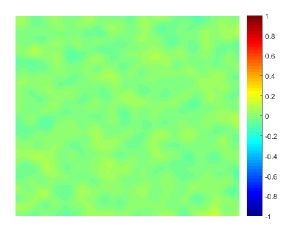
We use the uniform rectangular mesh with size for partition of the domain in this example and a random data ranging from to is generated on the mesh as the initial configuration of . The spatial discretization is done through the central finite difference as Example 2.7 so that the FFT can be used here for fast calculations needed in the ETDRK2 scheme. We set and in (18). According to Example 2.2, the positive root of is and the stabilizing constant is thus chosen as .
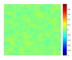
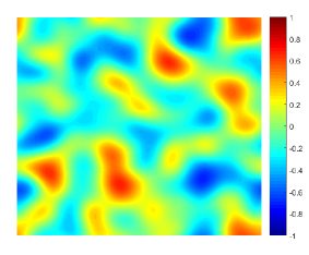
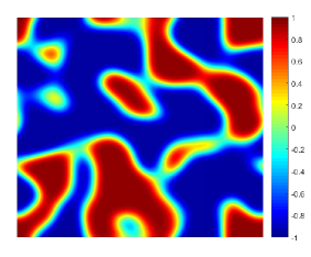
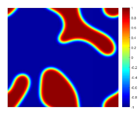
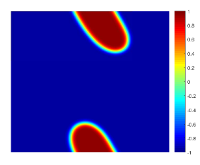
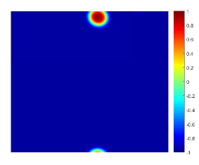
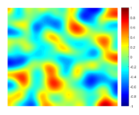
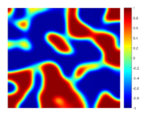
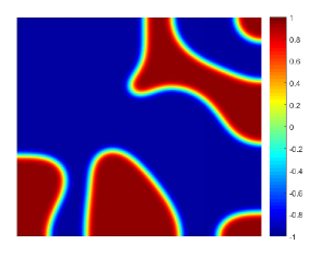
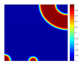
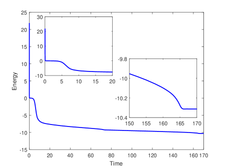
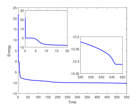
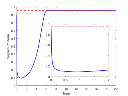
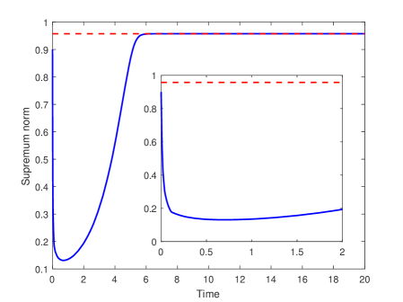
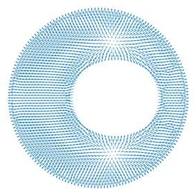
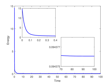
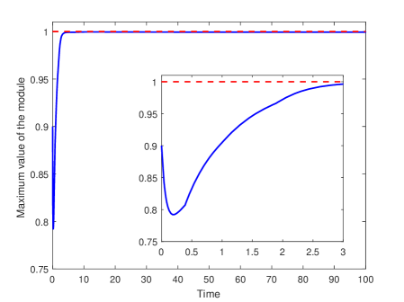
Fig. 1 shows the configurations of the approximate solution at , , , , , and subject to the periodic boundary condition. The simulation results illustrate the dynamics beginning with a random state and towards the homogeneous steady state of , which is reached after about in our simulations. The evolution of the energy is plotted in Fig. 3-(left) and that of the supremum norm of in Fig. 4-(left). The simulation results subject to the homogeneous Neumann boundary condition are presented in Fig. 2, where the same homogeneous steady state is reached after about . Fig. 3-(right) and Fig. 4-(right) show the corresponding evolutions of the energy and the supremum norm respectively. We observe that the energy decreases monotonically under both boundary conditions and the MBP is also preserved perfectly so that the solution is always located in the interval .

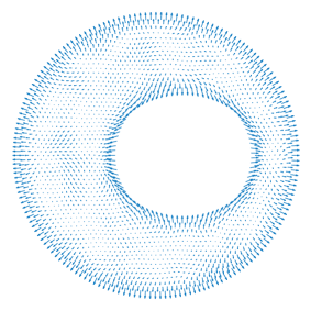
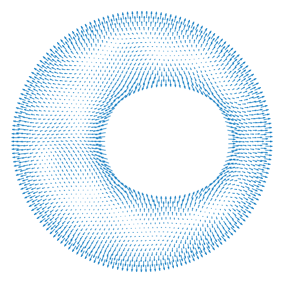
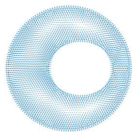
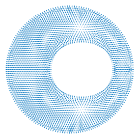
Example 5.2.
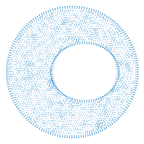
Consider the vector-valued equation (58) of the unknown vector field with replaced by . We test the domain
that is, a region inside the unit disk but outside a circle with a shifted center. The Dirichlet boundary condition is set to be
i.e., the values of the vector field on the outside boundary are always fixed to be a unit vector in the direction of and on the inside boundary be a unit vector in the direction of . Thus the winding number of the boundary is .
We adopt the finite element spatial discretization with piecewise linear basis functions on triangular meshes and the mass-lumping technique in this example. The stabilizing constant is set to be . PHIPM [77] is used for computing linear combinations of the products of the -functions with vectors in the ETDRK2 scheme. We generate a triangular mesh with nodes and elements for the domain and the initial configuration of the vector field on the interior nodes with the fixed magnitude but random directions according to a uniform distribution. Fig. 5 shows the simulated vector fields at , , , , , and respectively. We observe that the initial disordered state quickly transitions into a more orderly structure which then asymptotically evolves to a steady state. The obtained steady state of the vector field contain two vortices/defects which are symmetric with respect to the -axis. The evolution of the energy is plotted in the left graph of Fig. 6 for this example and we see the energy decreases monotonically in time. The right figure in Fig. 6 presents the evolution of the maximum value of over the interior nodes and it demonstrates again that the MBP is perfectly preserved.
6 Concluding remarks
In this work, we establish an abstract mathematical framework for studying MBPs of a class of semilinear parabolic equations subject to a variety of boundary conditions, as well as unconditionally MBP-preserving temporal approximation schemes, ETD1 and ETDRK2, based on the exponential integrator with a suitably chosen generator of a contraction semigroup. The motivation is to reveal essential characteristics of the semilinear parabolic equations having the MBPs and to analyze the fundamental conditions under which the ETD schemes unconditionally preserve the MBPs of the underlying problems. We conclude that, to ensure the MBP of the model equation (5) and the ETD schemes, a crucial condition is the dissipation property of the linear operator stated in Assumption 1 and the sign change property of the nonlinear term stated in Assumption 2. The main results presented in this paper significantly generalize those in [20] in many aspects. The existence of MBP-preserving ETDRK schemes of even higher-order defined in other approaches is an open question and remains as one of our future works.
Extensions of the framework to the cases of complex-valued, real vector-valued and matrix-valued equations in the space-continuous setting are also carried out by considering the nonlinear operators taking the double-well-like forms and either Dirichlet, homogeneous Neumann, or periodic boundary condition, where the MBPs are proposed with respect to the vector and matrix -norms, respectively. We also note that whether the matrix-valued equation (64) with nonhomogeneous Dirichlet boundary condition has the MBP with respect to the matrix -norm is still an open question and needs to be further studied. The main difficulty resides in that the matrix -norm of the matrix case behaves essentially differently from the absolute value in the scalar case or the magnitude in the vector case. Moreover, it is worth noting that the matrix-valued equation (64) is derived in [79] as the gradient flow under some energy functional with the nonlinear part as a penalty term for matrix-valued fields which do not take orthogonal matrix values. The penalty term takes the form , measuring the difference between a matrix and an orthogonal matrix in the sense of Frobenius norm (-norm), so it seems more natural to consider the MBP with respect to the -norm. Actually, it is not hard to prove that, if the -norm of the initial data is not greater than , then nor is the solution of the equation (64) at any time. However, unlike the case of -norm, the boundedness of the -norm of the solution is not sufficient to bound the nonlinear part in the splitting form; thus, whether this -norm-based MBP could be preserved by the ETD schemes is still an open question.
It is also worth mentioning that, apart from the ETD method, the integrating factor (IF) method is also a widely-used temporal integration method based on exponential integrators. While the ETD method only approximates the nonlinear terms as mentioned above, the IF method often applies numerical quadrature rules to the whole integrand. The IF method was introduced by Lawson [64] to solve ODE systems with large Lipschitz constants and applied to some problems with stiff linear part and nonstiff nonlinear part, such as the reaction-diffusion problems [56, 68, 76] and the advection-diffusion problems [53, 70, 106]. Due to highly different decaying rates of the exponential integrator components, the ETD schemes are usually more accurate than the IF ones for highly stiff systems. It is also the case that, if the nonlinear function is given by a constant (e.g., ), the ETD schemes can produce the exact solution to (1) while only approximate solutions are obtained by the IF schemes. One may ask whether, similar to ETD schemes, the IF schemes could preserve the MBPs. Related to this question, the authors of [53] focused on the property of strong stability-preserving (SSP) [42] for the IF Runge–Kutta (IFRK) schemes. SSP is a stronger stability than the MBP considered here. In fact, if we weaken the assumptions given in [53] appropriately, we could obtain MBP-preserving IFRK schemes under some suitable constraint on the time step size. Recall that a scheme is SSP means that if the linear operator satisfies
| (70) |
which is exactly Lemma 1-(ii), and there exists some such that the nonlinear mapping satisfies
| (71) |
then the solution always satisfies for any . Instead of (71), if one makes an assumption on as follows:
| (72) |
which is actually equivalent to Lemma 2-(i) with , With slight modifications to the proof for the IFRK schemes in [53], one can also conclude that the IFRK schemes, which are SSP under the conditions (70) and (71), are also MBP-preserving under the assumptions (70) and (72) (or say, Assumptions 1 and 2). Note that such property of MBP-preserving is only conditional in the sense that some constraint on the time step size is necessary. An open question is whether the MBP could be preserved unconditionally by the IF schemes as the ETD schemes if an appropriate stabilizer is introduced and this also remains as one of our future works.
Acknowledgements
The authors would like to thank the anonymous reviewers for their constructive comments and suggestions, which have helped us greatly improve this work. The authors are also grateful to Dr. Xiaochuan Tian of University of Texas at Austin and Dr. Zhi Zhou of The Hong Kong Polytechnic University for many valuable discussions.
References
- [1] S. M. Allen and J. W. Cahn, A microscopic theory for antiphase boundary motion and its application to antiphase domain coarsening, Acta Metall., 27 (1979), pp. 1085–1095.
- [2] H. Amann, Invariant sets and existence theorems for semilinear parabolic and elliptic systems, J. Math. Anal. Appl., 65 (1978), pp. 432–467.
- [3] S. Badia and A. Hierro, On discrete maximum principles for discontinuous Galerkin methods, Comput. Methods Appl. Mech. Engrg., 286 (2015), pp. 107–122.
- [4] G. Beylkin, J. M. Keiser, and L. Vozovoi, A new class of time discretization schemes for the solution of nonlinear PDEs, J. Comput. Phys., 147 (1998), pp. 362–387.
- [5] J. H. Bramble and B. E. Hubbard, New monotone type approximations for elliptic problems, Math. Comp., 18 (1964), pp. 349–367.
- [6] J. H. Brandts, S. Korotov, and M. Křížek, The discrete maximum principle for linear simplicial finite element approximations of a reaction-diffusion problem, Linear Algebra Appl., 429 (2008), pp. 2344–2357.
- [7] E. Burman and A. Ern, Discrete maximum principle for Galerkin approximations of the Laplace operator on arbitrary meshes, C. R. Math. Acad. Sci. Paris, Ser. I 338 (2004), pp. 641–646.
- [8] E. Chasseigne, The Dirichlet problem for some nonlocal diffusion equations, Differential Integral Equations, 20 (2007), pp. 1389–1404.
- [9] P. G. Ciarlet, Discrete maximum principle for finite-difference operators, Aequations Math., 4 (1970), pp. 338–352.
- [10] P. G. Ciarlet and P. A. Raviart, Maximum principle and uniform convergence for the finite element method, Comput. Methods Appl. Mech. Engrg., 2 (1973), pp. 17–31.
- [11] S. M. Cox and P. C. Matthews, Exponential time differencing for stiff systems, J. Comput. Phys., 176 (2002), pp. 430–455.
- [12] Q. Du, Global existence and uniqueness of solutions of the time-dependent Ginzburg–Landau model for superconductivity, Appl. Anal., 53 (1994), pp. 1–17.
- [13] Q. Du, Discrete gauge invariant approximations of a time-dependent Ginzburg–Landau model of superconductivity, Math. Comp., 67 (1998), pp. 965–986.
- [14] Q. Du, Numerical approximations of the Ginzburg–Landau models for superconductivity, J. Math. Phys., 46 (2005), Art. 095109.
- [15] Q. Du, Nonlocal Modeling, Analysis, and Computation, Vol. 94 of CBMS-NSF regional conference series in Applied Mathematics, SIAM, 2019.
- [16] Q. Du and X. B. Feng, The phase field method for geometric moving interfaces and their numerical approximations, in Geometric Partial Differential Equations - Part I, Handbook of Numerical Analysis, Vol. 21, Elsevier, 2020.
- [17] Q. Du, M. Gunzburger, R. B. Lehoucq, and K. Zhou, Analysis and approximation of nonlocal diffusion problems with volume constraints, SIAM Rev., 54 (2012), pp. 667–696.
- [18] Q. Du, M. Gunzburger, R. B. Lehoucq, and K. Zhou, A nonlocal vector calculus, nonlocal volume-constrained problems, and nonlocal balance laws, Math. Models Methods Appl. Sci., 23 (2013), pp. 493–540.
- [19] Q. Du, M. Gunzburger, and J. Peterson, Analysis and approximation of Ginzburg–Landau models for superconductivity, SIAM Rev., 34 (1992), pp. 54–81.
- [20] Q. Du, L. Ju, X. Li, and Z. H. Qiao, Maximum principle preserving exponential time differencing schemes for the nonlocal Allen–Cahn equation, SIAM J. Numer. Anal., 57 (2019), pp. 875–898.
- [21] Q. Du, R. Nicolaides, and X. Wu, Analysis and convergence of a covolume approximation of the Ginzburg–Landau model of superconductivity, SIAM J. Numer. Anal., 35 (1998), pp. 1049–1072.
- [22] Q. Du, Y. Z. Tao, X. C. Tian, and J. Yang, Asymptotically compatible discretization of multidimensional nonlocal diffusion models and approximation of nonlocal Green’s functions, IMA J. Numer. Anal., 39 (2019), pp. 607–625.
- [23] Q. Du and X. B. Yin, A conforming DG method for linear nonlocal models with integrable kernels, J. Sci. Comput., 80 (2019), pp. 1913–1935.
- [24] Q. Du and W.-X. Zhu, Analysis and applications of the exponential time differencing schemes and their contour integration modifications, BIT Numer. Math., 45 (2005), pp. 307–328.
- [25] S. W. Duo, H. W. van Wyk, and Y. Z. Zhang, A novel and accurate finite difference method for the fractional Laplacian and the fractional Poisson problem, J. Comput. Phys., 355 (2018), pp. 233–252.
- [26] S. W. Duo and Y. Z. Zhang, Accurate numerical methods for two and three dimensional integral fractional Laplacian with applications, Comput. Methods Appl. Mech. Engrg., 355 (2019), pp. 639–662.
- [27] K.-J. Engel and R. Nagel, One-Parameter Semigroups for Linear Evolution Equations, Graduate Texts in Mathematics, Vol. 194, Springer-Verlag, New York, 2000.
- [28] L. C. Evans, Partial Differential Equations, American Mathematical Society, Providence, Rhode Island, 2000.
- [29] L. C. Evans, H. M. Soner, and P. E. Souganidis, Phase transitions and generalized motion by mean curvature, Commun. Pure Appl. Math., 45 (1992), pp. 1097–1123.
- [30] I. Faragó and R. Horváth, Discrete maximum principle and adequate discretizations of linear parabolic problems, SIAM J. Sci. Comput., 28 (2006), pp. 2313–2336.
- [31] I. Faragó, J. Karátson, and S. Korotov, Discrete maximum principles for nonlinear parabolic PDE systems, IMA J. Numer. Anal., 32 (2012), pp. 1541–1573.
- [32] I. Faragó, S. Korotov, and T. Szabó, On continuous and discrete maximum principles for elliptic problems with the third boundary condition, Appl. Math. Comput., 219 (2013), pp. 7215–7224.
- [33] I. Faragó, S. Korotov, and T. Szabó, On continuous and discrete maximum-minimum principles for reaction-diffusion problems with the Neumann boundary condition, Applications of mathematics, pp. 34–44, Czech. Acad. Sci., Prague, 2015.
- [34] X. B. Feng and A. Prohl, Numerical analysis of the Allen–Cahn equation and approximation for mean curvature flows, Numer. Math., 94 (2003), pp. 33–65.
- [35] X. B. Feng and A. Prohl, Error analysis of a mixed finite element method for the Cahn–Hilliard equation, Numer. Math., 99 (2004), pp. 47–84.
- [36] X. Fernández-Real and X. Ros-Oton, Boundary regularity for the fractional heat equation, Rev. R. Acad. Cienc. Exactas Fís. Nat. Ser. A Mat., 110 (2016), pp. 49–64.
- [37] M. Frittelli, A. Madzvamuse, I. Sgura, and C. Venkataraman, Preserving invariance properties of reaction-diffusion systems on stationary surfaces, IMA J. Numer. Anal., 39 (2019), pp. 235–270.
- [38] E. Gallopoulous and Y. Saad, Efficient solution of parabolic equations by Krylov approximation methods, SIAM J. Sci. Comput., 13 (1992), pp. 1236–1264.
- [39] S. Gaudreault and J. A. Pudykiewicz, An efficient exponential time integration method for the numerical solution of the shallow water equations on the sphere, J. Comput. Phys., 322 (2016), pp. 827–848.
- [40] S. Gaudreault, G. Rainwater, and M. Tokman, KIOPS: A fast adaptive Krylov subspace solver for exponential integrators, J. Comput. Phys., 372 (2018), pp. 236–255.
- [41] V. Ginzburg and L. Landau, On the theory of superconductivity, Zh. Eksperim. Teor. Fiz., 20 (1950), pp. 1064–1082.
- [42] S. Gottlieb, C.-W. Shu, and E. Tadmor, Strong stability-preserving high-order time discretization methods, SIAM Rev., 43 (2001), pp. 89–112.
- [43] J.-L. Guermond, B. Popov, and L. Saavedra, Second-order invariant domain preserving ALE approximation of hyperbolic systems, J. Comput. Phys., 401 (2020), Art. 108927.
- [44] J.-L. Guermond, B. Popov, and I. Tomas, Invariant domain preserving discretization-independent schemes and convex limiting for hyperbolic systems, Comput. Methods Appl. Mech. Engrg., 347 (2019), pp. 143–175.
- [45] N. J. Higham, Functions of Matrices: Theory and Computation, SIAM, Philadelphia, PA, 2008.
- [46] M. Hochbruck and C. Lubich, On Krylov subspace approximations to the matrix exponential operator, SIAM J. Numer. Anal., 34 (1997), pp. 1911–1925.
- [47] M. Hochbruck, C. Lubich, and H. Selhofer, Exponential integrators for large systems of differential equations, SIAM J. Sci. Comput., 19 (1998), pp. 1552–1574.
- [48] M. Hochbruck and A. Ostermann, Explicit exponential Runge–Kutta methods for semilinear parabolic problems, SIAM J. Numer. Anal., 43 (2005), pp. 1069–1090.
- [49] M. Hochbruck and A. Ostermann, Exponential integrators, Acta Numer., 19 (2010), pp. 209–286.
- [50] R. A. Horn and C. R. Johnson, Topics in Matrix Analysis, Cambridge University Press, Cambridge, 1991.
- [51] T. L. Hou, T. Tang, and J. Yang, Numerical analysis of fully discretized Crank–Nicolson scheme for fractional-in-space Allen–Cahn equations, J. Sci. Comput., 72 (2017), pp. 1214–1231.
- [52] Y. H. Huang and A. Oberman, Numerical methods for the fractional Laplacian: a finite difference-quadrature approach, SIAM J. Numer. Anal., 52 (2014), pp. 3056–3084.
- [53] L. Isherwood, Z. J. Grant, and S. Gottlieb, Strong stability preserving integrating factor Runge–Kutta methods, SIAM J. Numer. Anal., 56 (2018), pp. 3276–3307.
- [54] Y. Jiang and H. L. Liu, Invariant-region-preserving DG methods for multi-dimensional hyperbolic conservation law systems, with an application to compressible Euler equations, J. Comput. Phys., 373 (2018), pp. 385–409.
- [55] L. Ju, X. Li, Z. H. Qiao, and H. Zhang, Energy stability and error estimates of exponential time differencing schemes for the epitaxial growth model without slope selection, Math. Comp., 87 (2018), pp. 1859–1885.
- [56] L. Ju, X. F. Liu, And W. Leng, Compact implicit integration factor methods for a family of semilinear fourth-order parabolic equations, Discrete Contin. Dyn. Syst. Ser. B, 19 (2014), pp. 1667–1687.
- [57] L. Ju, J. Zhang, and Q. Du, Fast and accurate algorithms for simulating coarsening dynamics of Cahn–Hilliard equations, Comput. Mater. Sci., 108 (2015), pp. 272–282.
- [58] L. Ju, J. Zhang, L. Y. Zhu, and Q. Du, Fast explicit integration factor methods for semilinear parabolic equations, J. Sci. Comput., 62 (2015), pp. 431–455.
- [59] A. Karafiat, Discrete maximum principle in parabolic boundary-value problems, Ann. Polon. Math., 53 (1991), pp. 253–265.
- [60] J. Karàtson and S. Korotov, Some discrete maximum principles arising for nonlinear elliptic finite element problems, Comput. Math. Appl., 70 (2015), pp. 2732–2741.
- [61] J. Karàtson, S. Korotov, and M. Křížek, On discrete maximum principles for nonlinear elliptic problems, Math. Comput. Simulation, 76 (2007), pp. 99–108.
- [62] D. R. Kassoy and J. Poland, The thermal explosion confined by a constant temperature boundary, SIAM J. Appl. Math., 39 (1980), pp. 412–430.
- [63] H. J. Kuiper, Invariant sets for nonlinear elliptic and parabolic systems, SIAM J. Math. Anal., 11 (1980), pp. 1075–1103.
- [64] J. D. Lawson, Generalized Runge–Kutta processes for stable systems with large Lipschitz constants, SIAM J. Numer. Anal., 4 (1967), pp. 372–380.
- [65] D. Li, Z. H. Qiao, and T. Tang, Characterizing the stabilization size for semi-implicit Fourier-spectral method to phase field equations, SIAM J. Numer. Anal., 54 (2016), pp. 1653–1681.
- [66] R. H. Li, Z. Y. Chen, and W. Wu, Generalized Difference Methods for Differential Equations: Numerical Analysis of Finite Volume Methods, Marcel Dekker, Inc., 2000.
- [67] Z. L. Li and K. Ito, Maximum principle preserving schemes for interface problems with discontinuous coefficients, SIAM J. Sci. Comput., 23 (2001), pp. 339–361.
- [68] X. F. Liu and Q. Nie, Compact integration factor methods for complex domains and adaptive mesh refinement, J. Comput. Phys., 229 (2010), pp. 5692–5706.
- [69] H. L. Liu and H. Yu, Maximum-principle-satisfying third order discontinuous Galerkin schemes for Fokker–Planck equations, SIAM J. Sci. Comput., 36 (2014), pp. A2296–A2325.
- [70] D. Lu and Y. T. Zhang, Computational complexity study on Krylov integration factor WENO method for high spatial dimension convection-diffusion problems, J. Sci. Comput., 73 (2017), pp. 980–1027.
- [71] E. C. MacRae, Matrix derivatives with an application to an adaptive linear decision problem, Ann. Statist., 2 (1974), pp. 337–346.
- [72] C. Mastroserio and M. Montrone, Invariant regions and asymptotic behaviour for the numerical solution of reaction-diffusion systems by a class of alternating direction methods, Calcolo, 21 (1984), pp. 269–279.
- [73] M. E. Mincsovics and T. L. Horváth, On the differences of the discrete weak and strong maximum principles for elliptic operators, Large-scale scientific computing, pp. 614–621, Lecture Notes in Comput. Sci., 7116, Springer, Heidelberg, 2012.
- [74] C. Moler and C. Van Loan, Nineteen dubious ways to compute the exponential of a matrix, SIAM Rev., 20 (1978), pp. 801–836.
- [75] C. Moler and C. Van Loan, Nineteen dubious ways to compute the exponential of a matrix, twenty-five years later, SIAM Rev., 45 (2003), pp. 3–49.
- [76] Q. Nie, F. Y. M. Wan, Y. T. Zhang, and X. F. Liu, Compact integration factor methods in high spatial dimensions, J. Comput. Phys., 227 (2008), pp. 5238–5255.
- [77] J. Niesen and W. M. Wright, Algorithm 919: A Krylov subspace algorithm for evaluating the -functions appearing in exponential integrators, ACM Trans. Math. Soft., 38 (2008), Art. 22.
- [78] R. H. Nochetto and W. J. Zhang, Discrete ABP estimate and convergence rates for linear elliptic equations in non-divergence form, Found. Comput. Math., 18 (2018), pp. 537–593.
- [79] B. Osting and D. Wang, A diffusion generated method for orthogonal matrix-valued fields, Math. Comp., 89 (2020), pp. 515–550.
- [80] E.-M. Ouhabaz, -contractivity of semigroups generated by sectorial forms, J. London Math. Soc., 46 (1992), pp. 529–542.
- [81] C. V. Pao, Nonlinear Parabolic and Elliptic Equations, Plenum Press, New York, 1992.
- [82] D.-Y. Peng and D. B. Robinson, A new two-constant equation of state, Ind. Eng. Chem. Fundamen., 15 (1976), pp. 59–64.
- [83] H. S. Price, Monotone and oscillation matrices applied to finite difference approximations, Math. Comp., 22 (1968), pp. 489–516.
- [84] Z. H. Qiao and S. Y. Sun, Two-phase fluid simulation using a diffuse interface model with Peng–Robinson equation of state, SIAM J. Sci. Comput., 36 (2014), pp. B708–B728.
- [85] R. Redheffer and W. Walter, Invariant sets for systems of partial differential equations. I. Parabolic equations, Arch. Rational Mech. Anal., 67 (1978), pp. 41–52.
- [86] W. Rudin, Principles of Mathematical Analysis, Third Edition, McGraw-Hill Book Co., New York, 1976.
- [87] S. G. Samko, A. A. Kilbas, and O. I. Marichev, Fractional Integrals and Derivatives, Gordon and Breach Science Publishers, Yverdon, 1993.
- [88] J. Shen, T. Tang, and J. Yang, On the maximum principle preserving schemes for the generalized Allen–Cahn equation, Commun. Math. Sci., 14 (2016), pp. 1517–1534.
- [89] J. Shen and X. F. Yang, Numerical approximations of Allen–Cahn and Cahn–Hilliard equations, Discrete Contin. Dyn. Syst., 28 (2010), pp. 1669–1691.
- [90] R. B. Sidje, Expokit: Software package for computing matrix exponentials, ACM Trans. Math. Soft., 24 (1998), pp. 130–156.
- [91] J. Smoller, Shock Waves and Reaction-Diffusion Equations, Fundamental Principles of Mathematical Sciences, Vol. 258, Second Edition, Springer-Verlag, New York, 1994.
- [92] P. Stehlík and J. Volek, Maximum principles for discrete and semidiscrete reaction-diffusion equation, Discrete Dyn. Nat. Soc., 2015, Art. 791304.
- [93] T. Tang and J. Yang, Implicit-explicit scheme for the Allen–Cahn equation preserves the maximum principle, J. Comput. Math., 34 (2016), pp. 471–481.
- [94] H. Tian, L. Ju, and Q. Du, Nonlocal convection-diffusion problems and finite element approximations, Comput. Methods Appl. Mech. Engrg., 289 (2015), pp. 60–78.
- [95] X. C. Tian and Q. Du, Analysis and comparison of different approximations to nonlocal diffusion and linear peridynamic equations, SIAM J. Numer. Anal., 51 (2013), pp. 3458–3482.
- [96] X. C. Tian, Q. Du, and M. Gunzburger, Asymptotically compatible schemes for the approximation of fractional Laplacian and related nonlocal diffusion problems on bounded domains, Adv. Comput. Math., 42 (2016), pp. 1363–1380.
- [97] R. S. Varga, On a discrete maximum principle, SIAM J. Numer. Anal., 3 (1966), pp. 355–359.
- [98] C. Wang, S. M. Wise, and J. S. Lowengrub, An energy-stable and convergent finite-difference scheme for the phase field crystal equation, SIAM J. Numer. Anal., 47 (2009), pp. 2269–2288.
- [99] X. Q. Wang, L. Ju, and Q. Du, Efficient and stable exponential time differencing Runge–Kutta methods for phase field elastic bending energy models, J. Comput. Phys., 316 (2016), pp. 21–38.
- [100] J. Yang, Q. Du, and W. Zhang, Uniform -bound of the Allen–Cahn equation and its numerical discretization, Int. J. Numer. Anal. Mod., 18 (2018), pp. 213–227.
- [101] P. Yang, T. Xiong, J. M. Qiu, and Z. F. Xu, High order maximum principle preserving finite volume method for convection dominated problems, J. Sci. Comput., 67 (2016), pp. 795–820.
- [102] E. G. Yanik, A discrete maximum principle for collocation methods, Comput. Math. Appl., 14 (1987), pp. 459–464.
- [103] E. G. Yanik, Sufficient conditions for a discrete maximum principle for high order collocation methods, Comput. Math. Appl., 17 (1989), pp. 1431–1434.
- [104] G. W. Yuan and Y. L. Yu, Existence of solution of a finite volume scheme preserving maximum principle for diffusion equations, Numer. Meth. Part. Diff. Eq., 34 (2018), pp. 80–96.
- [105] J. Zhang, C. B. Zhou, Y. G. Wang, L. Ju, Q. Du, X. B. Chi, D. S. Xu, D. X. Chen, Y. Liu, and Z. Liu, Extreme-scale phase field simulations of coarsening dynamics on the Sunway Taihulight supercomputer, in Proceedings of the International Conference for High Performance Computing, Networking, Storage and Analysis (SC’16), 2016, Art. 4.
- [106] S. Zhao, J. Ovadia, X. F. Liu, Y. T. Zhang, and Q, Nie, Operator splitting implicit integration factor methods for stiff reaction-diffusion-advection systems, J. Comput. Phys., 230 (2011), pp. 5996–6009.
- [107] L. Y. Zhu, L. Ju, and W. D. Zhao, Fast high-order compact exponential time differencing Runge–Kutta methods for second-order semilinear parabolic equations, J. Sci. Comput., 67 (2016), pp. 1043–1065.